On the controllability of some steady states in the case of nonlinear discrete dynamical systems with control

Abstract

The main objective of this paper is to show that two asymptotically stable steady states which belong to an analytic path of asymptotically stable steady states can be gradually transferred one to the other by successive changes of the control parameters.

¹Department of Mathematics, West University of Timişoara, Romania e-mail: balint@balint.uvt.ro

²Department of Physics, West University of Timişoara, Romania

³L.A.G.A, Institut Galilee, Universite Paris 13, France

1 Introduction

For nonlinear systems of differential equations with control, it has been proved (see [1]), that two asymptotically stable steady states belonging to an analytic path of asymptotically stable steady states can be transferred one in the other by successive maneuvers along the path. That means, according to [11], that the process described by the system can be piloted through the domains of attraction of the intermediary steady states, from the first to the second steady state.

In this paper, a similar result is established for the nonlinear discrete dynamical systems with control. A theorem from [4] is used, which states that the domain of attraction of an asymptotically stable fixed point of a nonlinear system of analytic difference equations, is the natural domain of analyticity of a certain Lyapunov function.

2 Preliminaries

We consider the following nonlinear discrete dynamical system with control:

$$x_{k+1}=f(x_{k},\alpha)\qquad k=0,1,2...$$ (1)

In (1), $f$ is a given function $f:\Omega\times D\rightarrow\mathbb{R}^{n}$, $\Omega\subset\mathbb{R}^{n}$, $D\subset\mathbb{R}^{m}$ are domains, $x\in\Omega$ is the state parameter, and $\alpha\in D$ is the control parameter. What concerns the regularity of $f$, we assume that $f$ is an analytic function.

A state $x^{0}\in\Omega$ is a steady state for (1) if there exists $\alpha_{x^{0}}\in D$ such that

$$x^{0}=f(x^{0},\alpha_{x^{0}})$$ (2)

The steady state $x^{0}\in\Omega$ of (1) is ”stable” provided that given any ball $B(x^{0},\varepsilon)=\{x\in\Omega/\|x-x^{0}\|<\varepsilon\}$, there is a ball $B(x^{0},\delta)=\{x\in\Omega/\|x-x^{0}\|<\delta\}$ such that if $x\in B(x^{0},\delta)$ then $f^{k}(x,\alpha_{x^{0}})\in B(x^{0},\varepsilon)$, for $k=0,1,2,...$ [5].

If in addition there is a ball $B(x^{0},r)$ such that $f^{k}(x,\alpha_{x^{0}})\rightarrow x^{0}$ as $k\rightarrow\infty$ for all $x\in B(x^{0},r)$ then the steady state $x^{0}$ is ”asymptotically stable” [5].

The domain of attraction $DA(x^{0})$ of the asymptotically stable steady state $x^{0}$ is the set of initial states $x\in\Omega$ from which the system converges to the steady state itself i.e.

$$DA(x^{0})=\{x\in\Omega|f^{k}(x,\alpha_{x^{0}})\stackrel{{\scriptstyle k\rightarrow\infty}}{{\longrightarrow}}x^{0}\}$$ (3)

An analytic path of steady states of (1) is an analytic function $\varphi:D_{1}\subset D\rightarrow\Omega$ which satisfies

$$\varphi(\alpha)=f(\varphi(\alpha),\alpha),\qquad\textrm{for any }\alpha\in D_{1}$$ (4)

An analytic path of asymptotically stable steady states of (1) is an analytic path of steady states which are all asymptotically stable.

A change of control parameters from $\alpha^{\prime}$ to $\alpha^{\prime\prime}$ in (1) is called maneuver and is denoted $\alpha^{\prime}\rightarrow\alpha^{\prime\prime}$. The maneuver $\alpha^{\prime}\rightarrow\alpha^{\prime\prime}$ is successful on the path $\varphi$ if $\alpha^{\prime},\alpha^{\prime\prime}\in D_{1}$ and the sequence defined by

$$x_{k+1}=f(x_{k},\alpha^{\prime\prime}),\textrm{ }x_{0}=\varphi(\alpha^{\prime})$$ (5)

tends to $\varphi(\alpha^{\prime\prime})$ as $k\rightarrow\infty$.

The following proposition from [4] concerning the discrete dynamical systems without control parameters is helpful.

Proposition 1.

If the analytic function $g:\Delta\rightarrow\Delta$ from the system

$$y_{k+1}=g(y_{k}),\qquad k=1,2,...$$ (6)

satisfies the following conditions:

$$g(0)=0$$ (7)

$$\|\partial_{0}g\|<1$$ (8)

then $0$ is an asymptotically stable steady state of (6). $DA(0)$ is an open subset of $\Delta$ and coincides with the natural domain of analyticity of the unique solution $V$ of the iterative first order functional equation

$$\begin{array}[]{ll}\left\{\begin{array}[]{l}V(g(y))-V(y)=-\|y\|^{2}\\ V(0)=0\end{array}\right.\end{array}$$ (9)

The function $V$ is positive on $DA(0)$ and $V(y)\stackrel{{\scriptstyle y\rightarrow y^{0}}}{{\longrightarrow}}+\infty$, for any $y^{0}\in FrDA(0)$ ($FrDA(0)$ denotes the boundary of $DA(0)$).

Remark 1.

If $\varphi:D_{1}\subset D\rightarrow\Omega$ is an analytical path of steady states of (1), then the function $g(\cdot,\alpha):\Omega-\varphi(\alpha)\rightarrow\Omega-\varphi(\alpha)$, given by

$$g(y,\alpha)=f(y+\varphi(\alpha),\alpha)-\varphi(\alpha)\qquad\textrm{for }y\in\Omega-\varphi(\alpha)$$ (10)

is analytic and satisfies $g(0,\alpha)=0$, for any $\alpha\in D_{1}$. Therefore, $y=0$ is a steady state of the system

$$y_{k+1}=g(y_{k},\alpha)\qquad k=0,1,2...\qquad\textrm{for any }\alpha\in D_{1}.$$ (11)

The steady state $x=\varphi(\alpha)$ of (1) is asymptotically stable if and only if the steady state $y=0$ of the system (11) is asymptotically stable. The relationship between the domain of attraction of the steady state $x=\varphi(\alpha)$ of (1) and that of the steady state $y=0$ of (11) is $DA(\varphi(\alpha))=\varphi(\alpha)+DA(0)$.

3 Theoretical results

We now state an existence theorem for an analytic path of asymptotically stable steady states of (1).

Theorem 1.

If the analytic function $f$ from (1) satisfies:

1. there exist $(x^{0},\alpha^{0})\in\Omega\times D$ such that $x^{0}=f(x^{0},\alpha^{0})$

2. $\|\partial_{x^{0}}f(x^{0},\alpha^{0})\|<1$

then there exists a maximal domain $D_{1}\subset D$ containing $\alpha^{0}$ and a unique analytic path $\varphi:D_{1}\rightarrow\Omega$ of asymptotically stable steady states of (1) satisfying the following conditions:

• $\varphi(\alpha^{0})=x^{0}$;

• $\|\partial_{x}f(\varphi(\alpha),\alpha)\|<1$ for any $\alpha\in D_{1}$;

• For $\alpha^{\prime},\alpha^{\prime\prime}\in D_{1}$ the maneuver $\alpha^{\prime}\rightarrow\alpha^{\prime\prime}$ is successful on the branch $\varphi$ if and only if $\varphi(\alpha^{\prime})$ belongs to the domain of attraction of $\varphi(\alpha^{\prime\prime})$.

Proof.

As the functions $f$ and $\partial_{x}f$ are continuous on $\Omega\times D$, taking into account the properties 1. and 2. of $f$, there exist two maximal domains $\Omega_{1}\subset\Omega$ and $D_{1}$ and a unique analytic function $\varphi:D_{1}\rightarrow\Omega_{1}$ such that:

1. $(x^{0},\alpha^{0})\in\Omega_{1}\times D_{1}$ and $\varphi(\alpha^{0})=x^{0}$;

2. $\varphi(\alpha)=f(\varphi(\alpha),\alpha)$, for any $\alpha\in D_{1}$;

3. $\|\partial_{x}f(\varphi(\alpha),\alpha)\|<1$ for any $\alpha\in D_{1}$.

This means that $\varphi$ is path of asymptotically stable steady states for (1) (see Proposition 1 and Remark 1).

A maneuver $\alpha^{\prime}\rightarrow\alpha^{\prime\prime}$ is successful on the path $\varphi$ if and only if the sequence given by (5) tends to $\varphi(\alpha^{\prime\prime})$ as $k\rightarrow\infty$, which means that $\varphi(\alpha^{\prime})$ belongs to the domain of attraction of $\varphi(\alpha^{\prime\prime})$. $\hbox to0.0pt{$\sqcap$\hss}\sqcup$

In the followings, it is assumed that the conditions of Theorem 1 are fulfilled and thus, there exists an analytic path $\varphi$ of asymptotically stable steady states of (1).

Theorem 2.

Let be $\varphi:D_{1}\rightarrow\Omega$ an analytic path of asymptotically stable steady states of (1). There exist an open set $G\subset\Omega\times D$ and a non-negative analytic function $V$ defined on $G$ satisfying the following conditions:

• $G\supset\Gamma=\{(\varphi(\alpha),\alpha)/\alpha\in D_{1}\}$

• $$\left\{\begin{array}[]{ll}V(f(x,\alpha),\alpha)-V(x,\alpha)=-\|x-\varphi(\alpha)\|^{2}\\ V(\varphi(\alpha),\alpha)=0\\ \end{array}\right.$$ (12)

• For any $\alpha\in D_{1}$, $DA(\varphi(\alpha))$ is the natural domain of analyticity of $x\rightarrow V(x,\alpha)$

• $V(x,\alpha)\stackrel{{\scriptstyle x\rightarrow x^{0}}}{{\longrightarrow}}+\infty$, for any $x^{0}\in FrDA(\varphi(\alpha))$.

Proof.

Let be $G=\bigcup\limits_{\alpha\in D_{1}}(DA(\varphi(\alpha))\times\{\alpha\})\subset\Omega\times D_{1}$ and $V:G\rightarrow\mathbb{R}^{1}_{+}$ defined by

$$V(x,\alpha)=\sum_{k=0}^{\infty}\|f^{k}(x,\alpha)-\varphi(\alpha)\|^{2}$$ (13)

Proposition 1 and Remark 1 provide that the set $G$ and the function $V(x,\alpha)$ satisfy the conditions a-d. $\hbox to0.0pt{$\sqcap$\hss}\sqcup$

Corollary 1.

If $\varphi:D_{1}\rightarrow\Omega$ is an analytic path of asymptotically stable steady states of (1) then for any $\alpha\in D_{1}$ there is an open neighborhood $U_{\alpha}$ of $\alpha$ and an open neighborhood $U_{\varphi(\alpha)}$ of $\varphi(\alpha)$ such that:

• $\varphi(\alpha^{\prime})\in U_{\varphi(\alpha)}$, for any $\alpha^{\prime}\in U_{\alpha}$;

• $U_{\varphi(\alpha)}\subset DA(\varphi(\alpha^{\prime}))$, for any $\alpha^{\prime}\in U_{\alpha}$

Proof.

For $\alpha\in D_{1}$ and $x\in DA(\varphi(\alpha))$, the function $V(x,\alpha)$ from Theorem 2 is considered. The real and non-negative function $V$ is defined on the open set $G=\bigcup\limits_{\alpha\in D_{1}}(DA(\varphi(\alpha))\times\{\alpha\})\subset\Omega\times D_{1}$, it is continuous and equal to zero on the set $\Gamma=\{(\varphi(\alpha),\alpha)/\alpha\in D_{1}\}\subset G$.

As $V$ is continuous and it is equal to zero in $(\varphi(\alpha),\alpha)\in G$, there is an open neighborhood $W$ of $(\varphi(\alpha),\alpha)$ such that for any $(x^{\prime},\alpha^{\prime})\in W$, the inequality $V(x^{\prime},\alpha^{\prime})<1$ holds. Let be $U_{\alpha}$ an open neighborhood of $\alpha$ and $U_{\varphi(\alpha)}$ of $\varphi(\alpha)$ such that $U_{\varphi(\alpha)}\times U_{\alpha}\subset W$. As the function $\varphi$ is continuous, it can be admitted that for any $\alpha^{\prime}\in U_{\alpha}$, we have $\varphi(\alpha^{\prime})\in U_{\varphi(\alpha)}$ (contrarily, the neighborhood $U_{\alpha}$ can be replaced with a smaller neighborhood $U_{\alpha}^{\prime}\subset U_{\alpha}$, for which we have $\varphi(\alpha^{\prime})\in U_{\varphi(\alpha)}$, for any $\alpha^{\prime}\in U_{\alpha}^{\prime}$).

Thus, for any $(x^{\prime},\alpha^{\prime})\in U_{\varphi(\alpha)}\times U_{\alpha}$, we have $V(x^{\prime},\alpha^{\prime})<1$. This means that for any $x^{\prime}\in U_{\varphi(\alpha)}$ and any $\alpha^{\prime}\in U_{\alpha}$, we have that $x^{\prime}\in DA(\varphi(\alpha^{\prime}))$. Thus, $U_{\varphi(\alpha)}\subset DA(\varphi(\alpha^{\prime}))$, for any $\alpha^{\prime}\in U_{\alpha}$. $\hbox to0.0pt{$\sqcap$\hss}\sqcup$

Remark 2.

Corollary 1 states that for any $\alpha^{\prime}\in U_{\alpha}$, both maneuvers $\alpha\rightarrow\alpha^{\prime}$ and $\alpha^{\prime}\rightarrow\alpha$ are successful on the path $\varphi$.

Theorem 3.

For two steady states $\varphi(\alpha^{\star})$ and $\varphi(\alpha^{\star\star})$ belonging to the analytic path $\varphi$ of asymptotically stable steady states of (1), there exist a finite number of values of the control parameters $\alpha^{1},\alpha^{2},...,\alpha^{p}\in D_{1}$ such that all the maneuvers

$$\alpha^{\star}\rightarrow\alpha^{1}\rightarrow\alpha^{2}\rightarrow...\rightarrow\alpha^{p}\rightarrow\alpha^{\star\star}$$ (14)

are successful on the path $\varphi$.

Proof.

Let be $P\subset D_{1}$ a polygonal line which joins $\alpha^{\star}$ and $\alpha^{\star\star}$. For any $\alpha\in P$ we consider the neighborhoods $U_{\alpha}$ and $U_{\varphi(\alpha)}$ given by Corollary 1.

The family of neighborhoods $\{U_{\alpha}\}_{\alpha\in P}$ is a covering with open sets of the compact polygonal line $P$. From this covering we can subtract a finite covering of $P$, i.e., there exist $\bar{\alpha}^{1},\bar{\alpha}^{2},...,\bar{\alpha}^{q}\in P$ such that $P\subset\bigcup\limits_{k=1}^{q}U_{\bar{\alpha}^{k}}$. More, it can be assumed that $\alpha^{\star}\in U_{\bar{\alpha}^{1}}$ and $\alpha^{\star\star}\in U_{\bar{\alpha}^{q}}$ and that the intersections $U_{\bar{\alpha}^{k}}\cap P$ are open and connected sets in $P$, and

$$(U_{\bar{\alpha}^{k}}\cap P)\cap(U_{\bar{\alpha}^{k+2}}\cap P)=\emptyset\qquad\textrm{for any }k=1,2,...,q-2.$$

Taking into account Remark 2, as $\alpha^{\star}\in U_{\bar{\alpha}^{1}}$ and $\alpha^{\star\star}\in U_{\bar{\alpha}^{q}}$, it comes naturally that the maneuvers $\alpha^{\star}\rightarrow\bar{\alpha}^{1}$ and $\bar{\alpha}^{q}\rightarrow\alpha^{\star\star}$ are successful on the path $\varphi$.

We still have to prove that each maneuver $\bar{\alpha}^{k}\rightarrow\bar{\alpha}^{k+1}$ is successful for any $k=1,2,...,q-1$.

If $\bar{\alpha}^{k}\in U_{\bar{\alpha}^{k+1}}$, Remark 2 provides that the maneuver $\bar{\alpha}^{k}\rightarrow\bar{\alpha}^{k+1}$ is successful on the path $\varphi$.

If $\bar{\alpha}^{k}\notin U_{\bar{\alpha}^{k+1}}$, a point $\bar{\alpha}^{k,k+1}\in(U_{\bar{\alpha}^{k}}\cap P)\cap(U_{\bar{\alpha}^{k+1}}\cap P)$ is considered. Remark 2 provides that both maneuvers $\bar{\alpha}^{k}\rightarrow\bar{\alpha}^{k,k+1}$ and $\bar{\alpha}^{k,k+1}\rightarrow\bar{\alpha}^{k+1}$ are successful on the path $\varphi$.

Thus, eventually inserting control parameters $\bar{\alpha}^{k,k+1}$ between $\bar{\alpha}^{k}$ and $\bar{\alpha}^{k+1}$, we come to find (after changing the notation and re-numbering) a finite sequence $\alpha^{1},\alpha^{2},...,\alpha^{p}\in D_{1}$ such that all the maneuvers

$$\alpha^{\star}\rightarrow\alpha^{1}\rightarrow\alpha^{2}\rightarrow...\rightarrow\alpha^{p}\rightarrow\alpha^{\star\star}$$

are successful on the path $\varphi$. $\hbox to0.0pt{$\sqcap$\hss}\sqcup$

Remark 3.

Theorem 3 states that two steady states belonging to an analytic path of asymptotically stable steady states can be transferred one in the other using a finite number of successful maneuvers along the considered path.

4 Numerical examples

Example 1.

The following one-dimensional discrete dynamical system with control is considered:

$$x_{k+1}=\alpha x_{k}(1-x_{k}),\qquad k=0,1,2,...$$ (15)

where $x\in\mathbb{R}$ is the state parameter and $\alpha\in\mathbb{R}$ is the control parameter. This dynamical system is frequently used for showing chaotic behavior and it is subject to several themes of research ([2]). We will illustrate using this system the concepts of analytic path, analytic path of asymptotically stable steady states, domain of attraction, successful maneuver.

For $\alpha\neq 0$, the steady states of (15) are $x=0$ and $x=\frac{\alpha-1}{\alpha}$, while for $\alpha=0$ corresponds only the $x=0$ steady state. Thus, for (15) there are three paths of steady states: $\varphi_{1}(\alpha)=\frac{\alpha-1}{\alpha}$, for $\alpha<0$, $\varphi_{2}(\alpha)=0$, for $\alpha\in\mathbb{R}$ and $\varphi_{3}(\alpha)=\frac{\alpha-1}{\alpha}$, for $\alpha>0$,. The path $\varphi_{1}$ contains only unstable steady states. The steady states belonging to the path $\varphi_{2}$ are asymptotically stable for $\alpha\in(-1,1)$. The steady states belonging to the path $\varphi_{3}$ are asymptotically stable for $\alpha\in(1,3)$.

In Fig. 1.2, the three paths of steady states are plotted. In Fig. 1.2 the gray rectangle represents the reunion of the domains of attraction of the asymptotically stable steady states of $\varphi_{3}$, while the vertical gray line denotes the domain of attraction of the steady state $\varphi_{2}(0)$. In both figures, the black parts of the paths of steady states represent the asymptotically stable steady states while the gray parts of the paths represent the unstable steady states.

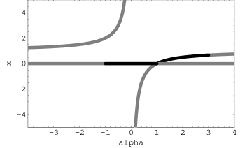
Figure 1.1: The paths of steady states for (15)

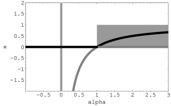
Figure 1.2: The domains of attractions of the asymptotically stable steady states of the path $\varphi_{3}$ and for the asymptotically stable steady state $\varphi_{2}(0)=0$ of $\varphi_{2}$

The domain of attraction of the steady state $\varphi_{2}(0)=0$ is $DA(\varphi_{2}(0))=\mathbb{R}$, while the domain of attraction of a steady state $\varphi_{3}(\alpha)$ for $\alpha\in(1,3)$ is $DA(\varphi_{3}(\alpha))=(0,1)$. These domains of attraction can be obtained using the staircase method [5], or can be estimated numerically using the method described in [4]).

The steady state $\varphi_{3}(1.1)$ can be directly transferred by a single maneuver to $\varphi_{3}(2.9)$, because $\varphi_{3}(1.1)\in DA(\varphi_{3}(2.9))=(0,1)$. The $DA(\varphi_{3}(1.1))$ includes $\varphi_{3}(2.9)$, thus, the maneuver $\alpha:2.9\rightarrow 1.1$ is also successful.

All asymptotically stable steady states of $\varphi_{3}$ are in the domain of attraction of the steady state $\varphi_{2}(0)$. This means that every maneuver $\alpha\rightarrow 0$, for $\alpha\in(1,3)$ is successful between the paths $\varphi_{3}$ and $\varphi_{2}$. Though, a steady state $\varphi_{2}(\alpha)$ cannot be transferred in an asymptotically stable steady state of $\varphi_{3}$, because any maneuver of the type $\alpha\rightarrow\alpha^{\prime}$, with $\alpha^{\prime}\in(1,3)$ causes a transfer to the unstable steady state $\varphi_{2}(\alpha^{\prime})=0$.

Example 2.

The following one-dimensional discrete dynamical system with control is considered:

$$x_{k+1}=(x_{k}-\alpha)^{3}+\alpha,\qquad k=0,1,2,...$$ (16)

where $x\in\mathbb{R}$ is the state parameter and $\alpha\in\mathbb{R}$ is the control parameter.

The sequence $x_{k}$, with the starting point $x_{0}$ which satisfies (16) is:

$$x_{k}=(x_{0}-\alpha)^{3^{k}}+\alpha,\qquad k=0,1,2,...$$ (17)

There are three analytic paths of steady states for (16): $\varphi_{1}(\alpha)=\alpha$, $\varphi_{2}(\alpha)=\alpha-1$ and $\varphi_{3}(\alpha)=\alpha+1$, defined for $\alpha\in\mathbb{R}$. The path $\varphi_{1}$ is an analytic path of asymptotically stable steady states while $\varphi_{2}$ and $\varphi_{3}$ are analytic paths of unstable steady states. In Fig. 3, the continuous line represents the path $\varphi_{1}$, while the dashed lines represent the paths $\varphi_{2}$ and $\varphi_{3}$.

For any $\alpha\in\mathbb{R}$, the domain of attraction of the asymptotically stable steady state $\varphi_{1}(\alpha)$ is $DA(\varphi_{1}(\alpha))=(\alpha-1,\alpha+1)$.

For $\alpha^{\star}=0$ and $\alpha^{\star\star}=2$, let’s consider the asymptotically stable steady states $\varphi_{1}(\alpha^{\star})=0$ and $\varphi_{1}(\alpha^{\star\star})=2$. The maneuver $\alpha:\alpha^{\star}=0\rightarrow 2=\alpha^{\star\star}$ is not successful, because $\varphi_{1}(\alpha^{\star})=0\notin DA(\varphi_{1}(\alpha^{\star\star})=2)=(1,3)$. Though, a finite number of maneuvers can be found, which transfer the steady state $\varphi_{1}(\alpha^{\star})=0$ to the steady state $\varphi_{1}(\alpha^{\star\star})=2$, for example:

$$\alpha:\alpha^{\star}=0\rightarrow 0.7\rightarrow 1.4\rightarrow 2=\alpha^{\star\star}$$ (18)

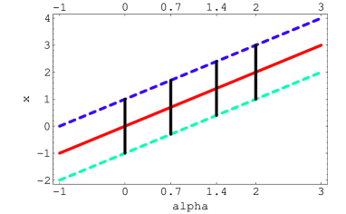
Figure 2: The paths of steady states for (16) and the domains of attraction of the steady states of $\varphi_{1}$ corresponding to the control parameters used in 18

These maneuvers are successful, because $\varphi_{1}(\alpha^{\star})\in DA(\varphi_{1}(0.7))=(-0.3,1.7)$, $\varphi_{1}(0.7)\in DA(\varphi_{1}(1.4))=(0.4,2.4)$ and $\varphi_{1}(1.4)\in DA(\varphi_{1}(\alpha^{\star\star}))=(1,2)$. In Fig. 3, the vertical segments represent the domains of attraction of the steady states corresponding to the maneuvers (18).

Example 3.

The following two-dimensional discrete dynamical system with control is considered:

$$\left\{\begin{array}[]{ll}x_{k+1}=(x_{k}-\alpha)[(x_{k}-\alpha)^{2}+(y_{k}-\alpha)^{2}]+\alpha\\ y_{k+1}=(y_{k}-\alpha)[(x_{k}-\alpha)^{2}+(y_{k}-\alpha)^{2}]+\alpha\\ \end{array}\right.$$ (19)

where $(x,y)\in\mathbb{R}^{2}$ is the state parameter and $\alpha\in\mathbb{R}$ is the control parameter.

There are an infinity of analytic paths of steady states for (19): $\varphi(\alpha)=(\alpha,\alpha)$ and $\varphi_{t}(\alpha)=(\alpha+\cos t,\alpha+\sin t)$, for $t\in[0,2\pi)$; all paths are defined for $\alpha\in\mathbb{R}$. The path $\varphi$ is an analytic path of asymptotically stable steady states while $\varphi_{t}$ are analytic paths of unstable steady states, for any $t\in[0,2\pi)$.

For any $\alpha\in\mathbb{R}$, the domain of attraction of the asymptotically stable steady state $\varphi(\alpha)=(\alpha,\alpha)$ is the ball $B((\alpha,\alpha),1)=\{(x,y)\in\mathbb{R}^{2}/(x-\alpha)^{2}+(y-\alpha)^{2}<1\}$.

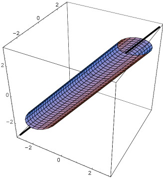
Figure 3: The paths of steady states for (19)

For $\alpha^{\star}=-1$ and $\alpha^{\star\star}=1$, let’s consider the asymptotically stable steady states $\varphi(\alpha^{\star})=(-1,-1)$ and $\varphi(\alpha^{\star\star})=(1,1)$. The maneuver $\alpha:\alpha^{\star}=-1\rightarrow 1=\alpha^{\star\star}$ is not successful, because $\varphi(\alpha^{\star})=(-1,-1)\notin DA(\varphi(\alpha^{\star\star})=(1,1))=B((1,1),1)$. Though, a finite number of maneuvers can be found, which transfer the steady state $\varphi(\alpha^{\star})=(-1,-1)$ to the steady state $\varphi(\alpha^{\star\star})=(1,1)$, for example:

$$\alpha:\alpha^{\star}=-1\rightarrow-0.5\rightarrow 0\rightarrow 0.5\rightarrow 1=\alpha^{\star\star}$$ (20)

These maneuvers are successful, because $\varphi(\alpha^{\star})\in DA(\varphi(-0.5))=B((-0.5,-0.5),1)$, $\varphi(-0.5)\in DA(\varphi(0))=B((0,0),1)$, $\varphi(0)\in DA(\varphi(0.5))=B((0.5,0.5),1)$, and $\varphi(0.5)\in DA(\varphi(\alpha^{\star\star}))=B((1,1),1)$.

References

- [1] St. Balint: Considerations concerning the maneuvering of some physical systems; An. Univ. Timisoara, Ser. St. Mat., vol. XXIII, (1985) p. 8-16.
- [2] M. Feigenbaum: Quantitative universality for a class of nonlinear transformations; J. Statist. Phys 19, (1978) p. 25-52.
- [3] L. Hörmander: An Introduction to Complex Analysis in Several Variables, D. Van Nostrand Company, Inc., Princeton, New Jersey
- [4] E. Kaslik, A.M. Balint, S. Birauas, St. Balint: Approximation of the domain of attraction of an asymptotically stable fixed point of a first order analytical system of difference equations. Nonlinear Studies, I&S Sience Publishers (2003).
- [5] W.G. Kelley, A.C. Peterson: Differene equations; Academic Press, 2001.
- [6] H. Kocak: Differential and Difference Equations Through Computer Experiments, Springer-Verlag, New York, 1990.
- [7] G. Ladas, C. Qian, P. Vlahos, J. Yan: Stability of solutions of linear nonautonomous difference equations. Appl. Anal. 41 (1991), no. 1-4, p. 183-191.
- [8] V. Lakshmikantham, D. Trigiante: Theory of Difference Equations: Numerical Methods and Aplications, Academic Press, New York, 1988.
- [9] J. LaSalle: Stablity theory for difference equations, MAA Studies in Mathematics 14, Studies in Ordinary Differntial Equations; edited by J. Hale, 1997, p. 1-31.
- [10] J. LaSalle: The Stability and Control of Discrete Processes, Springer-Verlag, New York, 1986.
- [11] V. Rasvan: Teoria Stabilitatii, Ed. Stiintifica si Enciclopedica (1987), Bucuresti.