Bootstrap Percolation on Infinite Trees and non-amenable groups

Abstract.

Bootstrap percolation on an arbitrary graph has a random initial configuration, where each vertex is occupied with probability $p$, independently of each other, and a deterministic spreading rule with a fixed parameter $k$: if a vacant site has at least $k$ occupied neighbors at a certain time step, then it becomes occupied in the next step. This process is well-studied on ${\mathbb{Z}}^{d}$; here we investigate it on regular and general infinite trees and on non-amenable Cayley graphs. The critical probability is the infimum of those values of $p$ for which the process achieves complete occupation with positive probability. On trees we find the following discontinuity: if the branching number of a tree is strictly smaller than $k$, then the critical probability is 1, while it is $1-1/k$ on the $k$-ary tree. A related result is that in any rooted tree $T$ there is a way of erasing $k$ children of the root, together with all their descendants, and repeating this for all remaining children, and so on, such that the remaining tree $T^{\prime}$ has branching number $\mbox{\rm br}(T^{\prime})\leq\max\{\mbox{\rm br}(T)-k,\,0\}$. We also prove that on any $2k$-regular non-amenable graph, the critical probability for the $k$-rule is strictly positive.

1. Introduction and results

Consider a countable, connected, locally finite graph $G=G(V,E)$, with two possible states for each site in the vertex set $V$: vacant (0) or occupied (1). Start with a configuration picked according to the product Bernoulli measure $\mathbb{P}_{p}$, i.e. each site is occupied randomly and independently with probability $p$. Then fix a parameter $k$, and consider the following deterministic spreading rule: if a vacant site has at least $k$ occupied neighbors at a certain time step, then it becomes occupied in the next step. This process is called bootstrap percolation. Complete occupation is the event that every vertex becomes occupied during the process. The main problem is to determine the critical probability $p(G,k)$ for complete occupation: for infinite graphs $G$ this is the infimum of the initial probabilities $p$ that make $\mathbb{P}_{p}$(complete occupation$)>0$. This model has a rich history in statistical physics, mostly on $G={\mathbb{Z}}^{d}$ and finite boxes; we will give some references later.

For infinite trees the most important characteristic of growth is the branching number $\mbox{\rm br}(T)$ of the tree, see [Lyo90] or [LP04]. It is defined as the supremum of real numbers $\lambda\geq 1$ such that $T$ admits a positive flow from the root to infinity, where on every edge $e\in E(T)$, the flow is bounded by $\lambda^{-|e|}$, and $|e|$ denotes the number of edges (including $e$) on the path from $e$ to the root. This supremum does not depend on the root, and remains unchanged if we modify a finite portion of the tree. Two basic examples are $\mbox{\rm br}(T_{k})=k$ for the $(k+1)$-regular tree, and $\mbox{\rm br}(T_{\xi})=\mathbb{E}\xi$ a.s. given non-extinction for the Galton-Watson tree $T_{\xi}$ with offspring distribution $\xi$. For finite trees, the branching number is 0.

On $T_{k}$, $k$-neighbor bootstrap percolation has $p(T_{k},k)=1-1/k$, see (1.4) in Proposition 1.2 below. In contrast, we have the following:

Theorem 1.1.

Let $T$ be an infinite tree. If $\mbox{\rm br}(T)<k$, then $p(T,k)=1$.

The above results show a somewhat surprising discontinuity of the function

$$f_{k}(b):=\inf\{p(T,k)\,:\,\mbox{\rm br}(T)\leq b,\ T\text{ has bounded degree}\}$$ (1.1)

at the value $b=k$. If we omit the condition of bounded degree, the discontinuity is even sharper: it is easy to construct a tree with $\mbox{\rm br}(T)=k$ and $p(T,k)=0$. A possible explanation of this discontinuity is given by Theorem 1.3 below.

For regular trees we give an equation for the critical probability, from which the actual value is more-or-less computable.

Proposition 1.2.

Let $2\leq k\leq d$. The critical probability $p(T_{d},k)$ is the supremum of all $p$ for which the equation

$$\mathbb{P}\bigl{(}{\rm Binom}(d,(1-x)(1-p))\leq d-k\bigr{)}=x$$ (1.2)

has a real root $x\in(0,1)$. In particular, for any constant $\gamma\in[0,1]$ and a sequence of integers $k_{d}$ with $\lim_{d\to\infty}{k_{d}}/{d}=\gamma$,

$$\lim_{d\to\infty}p(T_{d},k_{d})=\gamma.$$ (1.3)

Furthermore, for the extreme values of the parameter $k$,

$$p(T_{d},d)=1-\frac{1}{d}\mbox{\qquad{\rm and}\qquad}p(T_{d},2)=1-\frac{(d-1)^{2d-3}}{d^{d-1}(d-2)^{d-2}}\sim\frac{1}{2d^{2}}.$$ (1.4)

There is a generalization of a weaker form of Theorem 1.1. For this we first have to introduce the following simple notion, which will also be central to our proofs.

Definition 1.1.

A finite or infinite connected subset $F\subseteq V$ of vertices is called a $k$-fort if each $v\in F$ has outdegree $\deg_{V\setminus F}(v)\leq k$. Here $\deg_{H}(v)=|\{w\in H:(v,w)\in E\}|$, for any $H\subseteq V$.

A key observation is that the failure of complete occupation by the $k$-neighbor rule is equivalent to the existence of a vacant $(k-1)$-fort in the initial configuration.

Theorem 1.3.

Let $T$ be an infinite tree. Then every vertex $x\in T$ is contained in a $k$-fort $F$ with $\mbox{\rm br}(F)\leq\max\{\mbox{\rm br}(T)-k,\,0\}$.

This means that after fixing any vertex as the root, we can erase $k$ children of it, together with all their descendants, and can repeat this for all the remaining children, and so on, so that this pruning process results in a required subtree $F$. It is interesting to note that the natural idea of pruning off the $k$ subtrees with the largest branching numbers at each generation does not work in general.

For $\mbox{\rm br}(T)<k$ we get a $(k-1)$-fort with $\mbox{\rm br}(F)<1$, which can happen only if $F$ is finite, so $\mbox{\rm br}(F)=0$. In fact, in Theorem 1.1 we prove that there are infinitely many finite $(k-1)$-forts of bounded size, which implies $p(T,k)=1$. The impossibility of $0<\mbox{\rm br}(F)<1$ might be viewed as the reason for the discontinuity of $f_{k}(b)$ at $b=k$, though we do not actually know continuity at other points. See Section 5 for more discussion and open problems.

An infinite graph $G$ has the anchored expansion property if for some fixed vertex $o\in V(G)$, the anchored Cheeger constant is positive:

$$0<\iota^{*}(G):=\liminf\left\{\frac{|\partial_{e}S|}{|S|}:o\in S\subset V,\ S\mbox{ is finite and connected}\right\},$$ (1.5)

where $\partial_{e}S$ is the set of edges in $E(G)$ with exactly one endpoint in $S$. It is easy to see that the value of $\iota^{*}(G)$ does not depend on the vertex $o$. This notion is implicit in [Tho92], and was defined explicitly by [BLS99]. For transitive graphs (such as Cayley graphs of finitely generated infinite groups) it coincides with the more familiar but less robust concept of non-amenability, where the infimum is taken over all finite connected subsets $S$. For background on non-amenability see [LP04] or [Lyo00], and on anchored expansion [HSS00] or [Vir00b].

Theorem 1.4.

Let $G_{d}$ be a $d$-regular graph. If $\iota^{*}(G_{d})+2k>d$, then $p(G_{d},k)>0$. In particular, if $G_{d}$ has the anchored expansion property, then $p(G_{d},\lceil d/2\rceil)>0$.

This result is sharp in the sense that there exists a 6-regular non-amenable Cayley graph $G_{6}$ with $p(G_{6},2)=0$, see Section 4. We will pose a possible characterization of amenability in Section 5.

The issue of positivity of the critical probability is simpler for the case of trees. For this, let us denote by $q(G,k)$ the infimum of initial probabilities for which, following the $k$-neighbor rule on $G$, there will be an infinite connected component of occupied vertices in the final configuration with positive probability. Clearly, $q(G,k)\leq p(G,k)$.

Proposition 1.5.

For any integer $d$, and $k\geq 2$, if $T$ is an infinite tree with maximum degree $d+1$, then $p(T,k)\geq q(T_{d},k)>0$.

The first inequality of this proposition follows immediately from viewing $T$ as a subgraph of $T_{d}$. The positivity of the critical probability $q(T_{d},k)$ will be proved using our proof of Proposition 1.2 and an idea from [How00].

Bootstrap percolation was first defined in the statistical physics literature in [CRL79], where the formulae of (1.4) were given. A variant of the model appeared in [CRL82]. The problem of complete occupation on ${\mathbb{Z}}^{2}$ was solved by [vEn87]. Schonmann proved [Sch92] that the critical probability $p({\mathbb{Z}}^{d},k)$ for bootstrap percolation is 0 for $k\leq d$ and is 1 for $k>d$. The process can also be considered on finite graphs, see e.g. [AiL88], [BB03] and [Hol03]. A short recent physics survey is [AdL03]. Bootstrap percolation also has connections to the dynamics of the Ising model at zero temperature; see [FSS02] for ${\mathbb{Z}}^{d}$, and [How00] for $T_{2}$.

We conclude this introduction by some basic observations.

If a graph $G$ satisfies $\mathbb{P}_{p}($complete occupation with the $k$-rule$)\in\{0,1\}$ for all $p\in[0,1]$, and so $\mathbb{P}_{p}($complete occupation of $G)=1$ for any $p>p(G,k)$, then we will say that the 0-1 law holds for $G$ with the $k$-rule.

For example, if the orbit of each vertex under the automorphism group of $G$ is infinite, then the product probability measure of the initial configuration is ergodic [LP04, Proposition 6.3], while complete occupation is an invariant property, hence it has probability 0 or 1. Furthermore, if there is a finite $(k-1)$-fort in such a $G$, we immediately have infinitely many copies of this, so $p(G,k)=1$. On the other hand:

Lemma 1.6.

If there are no finite $(k-1)$-forts in a graph $G$, then $p(G,k)\leq 1-p_{c}(G)$, where $p_{c}(G)$ denotes the critical probability for standard site percolation on $G$.

Proof.

In the case of no complete occupation, the vacant $(k-1)$-fort has to be infinite, thus we have an infinite connected vacant component in the initial configuration. To have this event with positive probability, the density of initial vacant sites has to be at least the critical probability $p_{c}(G)$. ∎

Therefore, if $p_{c}(G)>0$ holds for a graph without finite $(k-1)$-forts, which is usually the case (e.g. if the degrees of vertices are bounded, see [LP04, Prop. 6.9]), then $p(G,k)<1$. For instance, on any tree $T$ we have $p_{c}(T)=1/\mbox{\rm br}(T)$, as was shown in [Lyo90].

We will say that a graph $G$ is uniformly bigger than a graph $H$ if every vertex of $G$ is contained in a subgraph of $G$ that is isomorphic to $H$.

Lemma 1.7.

(Monotonicity) If a graph $G$ is uniformly bigger than $H$, and $H$ satisfies the 0-1 law for some $k$-rule, then we have $p(G,k)\leq p(H,k)$.

Proof.

For any $p>p(H,k)$, any fixed vertex $v$ of $G$ becomes occupied almost surely, because of the copy of $H$ containing $v$. There are countably many vertices of $G$, so we have $\mathbb{P}_{p}($complete occupation of $G)=1$ with this $p$. ∎

In particular, if $T$ is a tree with maximal degree $d+1$ and it satisfies the 0-1 law, then we get $p(T,k)\geq p(T_{d},k)$. Proposition 1.5 is a generalization of this fact. We thank Ádám Timár for pointing out the importance of considering $q(T_{d},k)$ for the generalization.

2. Regular trees

Proof of Proposition 1.2. Consider the $(d+1)$-regular tree $T_{d}$, and fix $2\leq k\leq d$. This tree has no finite $(k-1)$-forts, and it is easy to see that any infinite fort of it contains a complete $(d+2-k)$-regular subtree. Hence, unsuccessful complete occupation for the $k$-rule is equivalent to the existence of a $(d+2-k)$-regular vacant subtree in the initial configuration.

Note that complete occupation on $T_{d}$ obeys the 0-1 law. So incomplete occupation has probability $1$ if and only if a fixed origin is contained in a $(d+2-k)$-regular vacant subtree with positive probability. Now a simple use of Harris’ inequality, see [LP04, Section 6.2], gives that this is equivalent to having the following event with positive probability: a $d$-ary tree, rooted at the fixed origin that is declared to be vacant, has a vacant $(d+1-k)$-ary subtree starting from the same root. Therefore, we need to determine when the connected component of vacant sites of the root, which is a random Galton-Watson tree with offspring distribution Binom$(d,1-p)$, contains a $(d+1-k)$-ary subtree with positive probability. If the probability of not having such a subtree is denoted by $y=y(p)$, then each of the $d$ children of the root has probability $1-p$ to be vacant, and given this event, has probability $1-y$ to be the root of a vacant $(d+1-k)$-ary subtree. Therefore, $y$ clearly satisfies the equation (1.2), i.e. it is a fixed point of the function

$$x\mapsto B_{d,k,p}(x) := \mathbb{P}\bigl{(}{\rm Binom}(d,(1-x)(1-p))\leq d-k\bigr{)}$$

$$= \sum_{j=0}^{d-k}{d\choose j}(1-x-p+xp)^{j}(p+x-px)^{d-j}.$$

One fixed point in $[0,1]$ is $x=1$; we are going to show that $y$ is actually the smallest one in $[0,1]$. It is easy to see that

$$\frac{\partial}{\partial x}B_{d,k,p}(x)=d(1-p)\mathbb{P}\bigl{(}{\rm Binom}(d-1,(1-x)(1-p))=d-k\bigr{)},$$

which is positive for $x\in[0,1)$, with at most one extremal point (a maximum) in $(0,1)$. Thus $B_{d,k,p}(x)$ is a monotone increasing function with $B_{d,k,p}(0)>0$ and with at most one inflection point in $(0,1)$. If $y_{n}$ denotes the probability that the required vacant subtree does not even reach the $n$th level below the root, then $y_{0}=0$, $y_{n+1}=B_{d,k,p}(y_{n})$, and $y_{n}\to y$. On the other hand, the sequence $y_{n}$ clearly approaches the smallest fixed point of $B_{d,k,p}(x)$, which so coincides with $y$. Thus, the infimum of the probabilities $p$ for which equation (1.2) has no positive real root $x<1$ is indeed the critical probability $p(T_{d},k)$.

If $\lim_{d\to\infty}{k_{d}}/{d}=\gamma$, then for any fixed $p$ and $x$, by the Weak Law of Large Numbers:

$$B_{d,k_{d},p}(x)=\mathbb{P}\left(\frac{{\rm Binom}(d,(1-x)(1-p))}{d}\leq\frac{d-k_{d}}{d}\right)\to\begin{cases}1,&\mbox{if\ }(1-x)(1-p)<1-\gamma\\ 0,&\mbox{if\ }(1-x)(1-p)>1-\gamma,\end{cases}$$

as $d\to\infty$. Solving the equation $(1-x)(1-p)=1-\gamma$ for $x$ gives a critical value $x_{c}=(\gamma-p)/(1-p)$. Thus for $p>\gamma$ we have $\lim_{d\to\infty}B_{d,k_{d},p}(x)\to 1$ for all $x\in[0,1]$, while for large enough $d$, $B_{d,k,p}(x)$ is convex in $[0,1]$, so there is no positive root $x<1$ of $B_{d,k_{d},p}(x)=x$. On the other hand, for $p<\gamma$ there must be a root $x=x(d)$ for large enough $d$, clearly satisfying $\lim_{d\to\infty}x(d)=x_{c}$. These prove (1.3).

The first equality of (1.4) follows immediately from (1.2). The second equality can be deduced by a standard calculus argument from our above formula for the first derivative of $B_{d,k,p}(x)$. ∎

Remark 1. We will use later that the extinction probability $y(p)$ introduced in the above proof satisfies $y(p)\to 0$ as $p\to 0$. This follows from the facts that $B_{d,k,0}(x)<x$ for $x>0$ small enough, that the functions $B_{d,k,p}(x)$ converge uniformly to $B_{d,k,0}(x)$ as $p\to 0$, and that $B_{d,k,p}(0)>0$.

Remark 2. A Galton-Watson tree with offspring distribution Binom$(d,1-p)$ can contain a $(d+1-k)$-ary subtree only if its mean is $(1-p)d\geq d+1-k$. Thus $p(T_{d},k)\leq\frac{k-1}{d}$ follows immediately.

Remark 3. The problem of finding regular subtrees in certain Galton-Watson trees was first considered in [CCD88], where the formula of (1.4) for $p(T_{9},2)$ was used. For general Galton-Watson processes, see [PD91]. From (1.3) it follows that the critical mean value for a binomial offspring distribution to produce an $N$-ary subtree in the Galton-Watson tree is asymptotically $N$. In [PD91] it was shown that this critical mean value is $\sim eN$ for a geometric offspring distribution, and $\sim N$ for a Poisson offspring. An interesting feature of these phase transitions is that unlike the case of usual percolation $N=1$, for $N\geq 2$ the probability of having the $N$-ary subtree is already positive at criticality. For bootstrap percolation this means that the probability of complete occupation is still 0 at $p=p(T_{d},k)$ if $k<d$.

Remark 4. The critical probability $p(T,k)$ can be computed also for quasi-transitive (periodic) trees and Galton-Watson trees, as we will see for example in Section 5.

Proof of Proposition 1.5. To prove the second inequality, $q(T_{d},k)>0$, we will first show that for any non-backtracking path $v_{0},v_{1},\dots,v_{n}$ in $T_{d}$,

$$\mathbb{P}_{p}\bigl{(}\{v_{0},\dots,v_{n}\}\mbox{ does not intersect any vacant }(k-1)\mbox{-fort}\bigr{)}\leq[1-z(p)^{2}]^{\lfloor n/2\rfloor},$$ (2.1)

where $z(p)$ is the probability that an infinite rooted tree $Z$ with $d-1$ children at the root, and $d$ children everywhere else, has a $(d+1-k)$-ary vacant subtree containing the root. Before proving (2.1), note that $z(p)\to 1$ as $p\to 0$. This follows easily from the fact $y(p)\to 0$ of Remark 1 above.

To prove (2.1), for each $v_{i}$ consider a copy $Z_{i}$ of $Z$ inside $T_{d}$, rooted at $v_{i}$, disjoint from the path $v_{0},\dots,v_{n}$. Then the subtrees $Z_{i}$ are also disjoint from each other. The $(d+1-k)$-ary vacant subtrees rooted at $v_{2i}$ and $v_{2i+1}$ inside $Z_{2i}$ and $Z_{2i+1}$ join together to give a vacant $(d+2-k)$-regular tree, i.e. a $(k-1)$-fort, inside $T_{d}$. The probability that this does not happen for any of the pairs $v_{2i},v_{2i+1}$ is exactly the RHS of (2.1).

The number of different paths $v_{0},v_{1},\dots,v_{n}$ from a fixed vertex $v_{0}=o$ is $(d+1)d^{n-1}$. Therefore, if $p$ is so small that $\sqrt{1-z(p)^{2}}<1/d$, then the probability that there is at least one such path that does not intersect any vacant $(k-1)$-forts in the initial configuration is exponentially small in $n$. By the Borel-Cantelli lemma, any infinite non-backtracking path from $o$ eventually intersects a vacant $(k-1)$-fort almost surely, hence the bootstrap percolation process will not be able to form an infinite occupied cluster containing $o$. There are countably many possible $o$ vertices in $T_{d}$, so we have the same for all vertices with probability 1. Thus $q(T_{d},k)\geq p$ with the above small $p>0$. ∎

3. General infinite trees

To start our discussion of the connection between branching number and bootstrap percolation, let us prove a simple combinatorial lemma, which implies Theorem 1.3 for the special case of $\mbox{\rm br}(T)<k$, but is not yet enough to prove Theorem 1.1.

Lemma 3.1.

(Red Lemma) If some vertex $x$ of a tree $T$ is not contained in any finite $(k-1)$-fort, then there is a $k$-ary subtree containing $x$.

Proof.

Consider the tree $T$ as rooted at the vertex $x$. First color red all vertices with at most $k-1$ children. In the second step, color red each vertex with at most $k-1$ non-red children, and repeat this over and over again; see Figure 1. In the limiting final coloring, if the root $x$ is red, then it obtained its color in a finite number of steps, so there is a finite set $F$ of vertices such that $x$ becomes red even if we fix all the vertices outside $F$ to be uncolored forever. If we take this $F$ to be minimal, then it is a finite connected subtree of $T$, with all leaves painted red in the first step, and all vertices becoming eventually red. But now, this red $F$ is clearly a finite $(k-1)$-fort in $T$, contradicting the choice of $x$. Therefore, $x$ is not red in the final limiting coloring. This means it has at least $k$ non-red children, and each of these children also has at least $k$ non-red children, and so on. Hence, the non-red component of $x$ in $T$ contains the $k$-ary subtree we wanted. ∎

Theorem 1.1 is not obvious from this lemma because if we do not forbid all finite $(k-1)$-forts, but only the appearance of too many small ones, we can already get $p(T,k)<1$, while we can have vertices with at most $k-1$ children lying close to each other (see the tree on the right in Figure 1), so $\mbox{\rm br}(T)<k$ could possibly occur, as well. Thus we need a quantitative version of Lemma 3.1. For this, fix a root $o$ for $T$, and denote by $L_{r}(x)$ the set of the vertices $y$ from which the shortest path to $o$ contains $x$, and $\mbox{\rm dist}(o,y)=\mbox{\rm dist}(o,x)+r$.

Lemma 3.2.

(Blue Lemma) Let $x$ be a vertex with $|L_{R}(x)|<(k-1)k^{R-1}$ for some positive integer $R$. Then $\cup_{0\leq r\leq R}L_{r}(x)$ contains a $(k-1)$-fort of $T$.

Proof.

Let $x$ be a vertex of the tree satisfying the conditions of the lemma, and label its level by $0$. Color a vertex on level $R$ blue, if it has at least $k$ children. In general, color a vertex on level $r$ blue, if it has at least $k$ blue children ($r<R$). The vertex $x$ is definitely not blue, otherwise $|L_{R}(x)|\geq k^{R}$ would hold. Moreover, $x$ has at most $k-2$ blue children, since $|L_{R}(x)|<(k-1)k^{R-1}$. If $x$ has less than $k-1$ children, then it is a fort by itself. Otherwise, the non-blue component containing $x$ contains at least $2$ vertices. We claim that the non-blue connected component containing $x$ is a $(k-1)$-fort. First of all, $x$ has outdegree at most $k-1$, counting its mother and its possible $k-2$ blue children. Any other vertex from this set has a non-blue mother, and being non-blue means that it has at most $k-1$ blue neighbors. A non-blue vertex in this component in the level $R$ has at most $k-1$ children, and its mother is not blue. ∎

Note that almost the same argument for $x=o$ gives that already $|L_{R}(o)|<k^{R}$ implies a $(k-1)$-fort inside $\cup_{0\leq r\leq R}L_{r}(o)$. (The reason for the strengthening is simple: $o$ does not have a mother.)

           

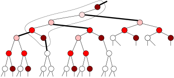
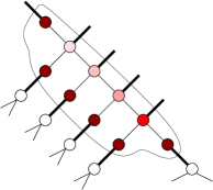
Figure 1. Some finite 1-forts.

Proof of Theorem 1.1. We will prove that if there is no $(k-1)$-fort with at most $N$ vertices, then $\mbox{\rm br}(T)\geq k-\frac{2k\log k}{\log N}$. This suffices because destroying a finite number of forts of size at most $N$ does not affect $\mbox{\rm br}(T)$, so $\mbox{\rm br}(T)<k$ will imply the existence of infinitely many $(k-1)$-forts of bounded size, which shows $p(T,k)=1$.

Any leaf of $T$ would be a $(k-1)$-fort with one vertex, so there are no leaves, and we have $|L_{r}(x)|\leq|L_{r+1}(x)|$ for any $r$ and $x$. Hence, the fort that the Blue Lemma finds for us has less than $Rk^{R}<k^{2R}$ vertices. Thus having no $(k-1)$-forts of size at most $N$ implies that $|L_{r}(x)|\geq(k-1)k^{r-1}$ and $|L_{r}(o)|\geq k^{r}$ for every $r\leq R=\frac{\log N}{2\log k}$. We will prove that if $\lambda>0$ is such that

$$\lambda^{R}\leq(k-1)k^{R-1},$$ (3.1)

then $\mbox{\rm br}(T)\geq\lambda$. For example, if $\lambda=k-\frac{c_{k}}{\log N}$, then $\lambda^{R}\leq N^{1/2}\exp(-\frac{c_{k}}{2k\log k})$, while $(k-1)k^{R-1}=\frac{k-1}{k}N^{1/2}$, so $c_{k}=2k\log k$ is good for any $k\geq 2$.

Now we have to show that if the capacity of an edge $e$ is $\lambda^{-|e|}$, then the network admits a positive flow from the root to infinity. Start the flow with an amount $k^{-R}$ at the root $o$. On level $R$ there are at least $k^{R}$ vertices; divide the initial amount equally among them, and build the flow from $o$ to $L_{R}(o)$ according to these amounts. Then through each edge before level $L_{R}(o)$ the amount that flows is at most the initial $k^{-R}$, while the capacity of such an edge is at least $\lambda^{-R}$, which is bigger because of (3.1). So this is an admissible flow from $o$ to $L_{R}(o)$.

The value of the flow at each vertex in $L_{R}(o)$ is at most $k^{-2R}$. For each such vertex $x$, we have $|L_{R}(x)|\geq(k-1)k^{R-1}$. Divide the amount at $x$ equally among these vertices, do the same for all $x\in L_{R}(o)$, and continue the flow from $L_{R}(o)$ to $L_{2R}(o)$ according to this. Through each edge between $L_{R}(o)$ and $L_{2R}(o)$ the amount that should flow is at most $k^{-2R}$, while the capacity of an edge is at least $\lambda^{-2R}$. Thus we have an admissible flow constructed already from $o$ to $L_{2R}(o)$.

Continuing in this manner: between the levels $L_{(n-1)R}(o)$ and $L_{nR}(o)$ the amount that should flow through an edge is at most $(k-1)^{-(n-2)}k^{-(nR-n+2)}$, and the capacity of such an edge is at least $\lambda^{-nR}$. This second is bigger because of (3.1), thus we have constructed an admissible flow from $o$ to infinity with the positive value $k^{-R}$. ∎

The converse is clearly false, as shown for example by a $(d+1)$-regular tree with an additional vertex placed on each of the edges. This tree $T_{d}^{\prime}$ has branching number $\sqrt{d}$, while any vertex of the original $T_{d}$ together with its $d+1$ neighbors form a $1$-fort of size $d+2$, so $p(T_{d}^{\prime},2)=1$. Furthermore, one might ask how sharp the above result $\mbox{\rm br}(T)\geq k-\frac{2k\log k}{\log N}$ is — see Section 5.

Proof of Theorem 1.3. Fix a vertex $x$ as the root of $T$. It is enough to prove the theorem for $k=1$, and thus find a small 1-fort $F_{1}$ in $T$ containing $x$, because then we can inductively find a 1-fort $F_{2}$ inside $F_{1}$ with $\mbox{\rm br}(F_{2})\leq\mbox{\rm br}(F_{1})-1\leq\mbox{\rm br}(T)-2$, which will also be a 2-fort in $T$, and so on.

By the Max-Flow-Min-Cut theorem, the branching number is characterized by

$$\mbox{\rm br}(T)=\sup\left\{\lambda:\inf_{\Pi}\sum_{e\in\Pi}\lambda^{-|e|}>0\right\},$$ (3.2)

where the $\inf$ is over cutsets $\Pi$ of edges separating $x$ from $\infty$. The expression $\mu_{\lambda}(\Pi):=\sum_{e\in\Pi}\lambda^{-|e|}$ will be called the $\lambda$-content of the cutset (or of an arbitrary set of edges).

Fix some $\beta>1$, and take an arbitrary finite tree ${\mathcal{T}}$ with root $r$. By its boundary $\partial{\mathcal{T}}$ we mean the set of edges with a leaf as an endpoint. If ${\mathcal{T}}=\{r\}$, then let $\mu_{\beta}(\partial{\mathcal{T}})=1$. Otherwise, denote the children of $r$ by $r_{1},\dots,r_{\ell}$. Deleting the edge $(r,r_{i})$ from ${\mathcal{T}}$ results in two connected components; the subtree that contains $r_{i}$ will be denoted by ${\mathcal{T}}_{i}$, and ${\mathcal{T}}_{i}$ together with $r$ by $\hat{\mathcal{T}}_{i}$. We have the disjoint union $\cup_{i=1}^{\ell}\partial\hat{\mathcal{T}}_{i}=\partial{\mathcal{T}}$, hence $m_{1}+\dots+m_{\ell}=\mu_{\beta}(\partial{\mathcal{T}})$, where $m_{i}:=\mu_{\beta}(\partial\hat{\mathcal{T}}_{i})$. We may assume $m_{1}\leq m_{2}\leq\dots\leq m_{\ell}$. Now let us delete from ${\mathcal{T}}$ the entire “$\beta$-largest” subtree ${\mathcal{T}}_{\ell}$. Then look at the subtrees ${\mathcal{T}}_{1},\dots,{\mathcal{T}}_{\ell-1}$, and repeat the whole procedure with each ${\mathcal{T}}_{i}$ instead of ${\mathcal{T}}$, with root $r_{i}$, deleting the “$\beta$-largest” subtree from each ${\mathcal{T}}_{i}$. Repeat this procedure over and over again until reaching the boundary of ${\mathcal{T}}$ in all subtrees. The remaining subtree ${\mathcal{F}}$ is clearly a 1-fort inside ${\mathcal{T}}$. We claim that

$$\mu_{\beta-1}(\partial{\mathcal{F}}\cap\partial{\mathcal{T}})\leq\mu_{\beta}(\partial{\mathcal{T}})^{\alpha},$$ (3.3)

where $\alpha=\beta/(\beta-1)$. Equality holds only for finite $\beta$-ary trees ${\mathcal{T}}$, for integer $\beta$.

Before proving this claim, we show how it implies the existence of an infinite 1-fort $F$ inside $T$, rooted at $x$, with $\mbox{\rm br}(F)\leq\mbox{\rm br}(T)-1$.

Take a strictly decreasing sequence of positive numbers $\{\beta_{n}\}$ converging to $\mbox{\rm br}(T)\geq 1$. Let $\alpha_{n}=\beta_{n}/(\beta_{n}-1)>1$. We can suppose that $T$ has no leaves. We have $\beta_{1}>\mbox{\rm br}(T)$, so by the characterization (3.2), for any $\epsilon_{1}>0$ there exists a cutset $\Pi^{1}$ separating $x$ from $\infty$ with $\mu_{\beta_{1}}(\Pi^{1})<\epsilon_{1}$. If the finite subtree between $x$ and $\Pi^{1}$ is called ${\mathcal{T}}^{1}$, then our above procedure finds a 1-fort ${\mathcal{F}}^{1}$ of ${\mathcal{T}}^{1}$, with $\mu_{\beta_{1}-1}(\partial{\mathcal{F}}^{1}\cap\Pi^{1})<\epsilon_{1}^{\alpha_{1}}$. This upper bound is less than $1/2$ if we choose $\epsilon_{1}=1/2$. Now denote the lower endvertices of the edges in $\partial{\mathcal{F}}^{1}\cap\Pi^{1}$ by $x_{1},\dots,x_{\ell}$. The infinite subtree of $T$ starting at $x_{i}$, called $T_{i}$, has branching number less than $\beta_{2}$. Hence, for each $i$ and any $\epsilon_{2}>0$, we can take a cutset $\Pi^{2}_{i}$ separating $x_{i}$ from $\infty$ with $\mu^{*}_{\beta_{2}}(\Pi^{2}_{i})<\epsilon_{2}$, where $\mu^{*}_{\beta_{2}}$ denotes $\beta_{2}$-content with distances $|e|$ measured from the new root $x_{i}$. That is, $\mu_{\beta_{2}}(\Pi^{2}_{i})<\epsilon_{2}\beta_{2}^{-|x_{i}|}$. If the finite subtree between $x_{i}$ and $\Pi^{2}_{i}$ is called ${\mathcal{T}}^{2}_{i}$, then our pruning procedure yields a 1-fort ${\mathcal{F}}^{2}_{i}$ inside each ${\mathcal{T}}^{2}_{i}$, satisfying $\mu^{*}_{\beta_{2}-1}(\partial{\mathcal{F}}^{2}_{i}\cap\Pi^{2}_{i})<\epsilon_{2}^{\alpha_{2}}$. If we take the union $\Phi^{2}:=(\partial{\mathcal{F}}^{2}_{1}\cap\Pi^{2}_{1})\cup\dots\cup(\partial{\mathcal{F}}^{2}_{\ell}\cap\Pi^{2}_{\ell})$, then $\mu_{\beta_{2}-1}(\Phi^{2})=\sum_{i=1}^{\ell}\mu_{\beta_{2}-1}(\partial{\mathcal{F}}^{2}_{i}\cap\Pi^{2}_{i})<\sum_{i=1}^{\ell}\epsilon_{2}^{\alpha_{2}}(\beta_{2}-1)^{-|x_{i}|}=\epsilon_{2}^{\alpha_{2}}\mu_{\beta_{2}-1}(\partial{\mathcal{F}}^{1}\cap\Pi^{1})$. Since $\mu_{\beta_{2}-1}(\partial{\mathcal{F}}^{1}\cap\Pi^{1})$ is a finite number independent of $\epsilon_{2}$, we can choose $\epsilon_{2}$ so small that the last upper bound is less than $1/4$. Now we repeat everything with the infinite subtrees of $T$ starting at the lower endvertices $\{y_{i},i=1,\dots,m\}$ of $\Phi^{2}$, using $\beta_{3}$ and some $\epsilon_{3}>0$. This gives a collection of cutsets $\{\Pi^{3}_{i}\}$ and finite 1-forts $\{{\mathcal{F}}^{3}_{i}\}$. Take the union $\Phi^{3}:=(\partial{\mathcal{F}}^{3}_{1}\cap\Pi^{3}_{1})\cup\dots\cup(\partial{\mathcal{F}}^{3}_{m}\cap\Pi^{3}_{m})$, and choose $\epsilon_{3}$ sufficiently small so that $\mu_{\beta_{3}-1}(\Phi^{3})<1/8$. Repeat this ad infinitum, choosing $\epsilon_{n}$ such that $\mu_{\beta_{n}-1}(\Phi^{n})<2^{-n}$.

The union of all the finite 1-fort-pieces, $F:={\mathcal{F}}^{1}\cup{\mathcal{F}}^{2}_{1}\cup\dots\cup{\mathcal{F}}^{2}_{\ell}\cup\dots$, is an infinite 1-fort of $T$, and each $\Phi^{n}$ is a cutset of $F$ separating $x$ from $\infty$. For any fixed $\beta>\mbox{\rm br}(T)$, if $n$ is large enough to have $\beta_{n}<\beta$, then $\mu_{\beta-1}(\Phi^{n})<\mu_{\beta_{n}-1}(\Phi^{n})<2^{-n}$. Thus, by definition (3.2), $\mbox{\rm br}(F)\leq\beta-1$. Since this holds for all $\beta>\mbox{\rm br}(T)$, we have proved $\mbox{\rm br}(F)\leq\mbox{\rm br}(T)-1$.

We prove (3.3) by induction on the depth of ${\mathcal{T}}$. If this depth is 1, i.e. each child $r_{i}$ of $r$ is a leaf, then ${\mathcal{F}}$ is just obtained by deleting $r_{\ell}$, so we need to prove $(\ell-1)/(\beta-1)\leq(\ell/\beta)^{\alpha}$. By taking derivatives with respect to $\ell$ it is easy to check that the only value of $\alpha$ for which this inequality holds for all real $\ell\geq 1$ is the chosen $\alpha=\beta/(\beta-1)$. Equality holds only for $\ell=\beta$.

Suppose inductively that inside each subtree ${\mathcal{T}}_{i}$, $i=1,\dots,\ell$, we have our 1-fort ${\mathcal{F}}_{i}$ with $\mu^{*}_{\beta-1}(\partial{\mathcal{F}}_{i}\cap\partial{\mathcal{T}}_{i})\leq m_{i}^{\alpha}$, where $\mu^{*}_{\lambda}$ denotes $\lambda$-content measured inside ${\mathcal{T}}_{i}$ with root $r_{i}$, and $m_{i}=\mu^{*}_{\beta}(\partial{\mathcal{T}}_{i})$. We get ${\mathcal{F}}$ by joining the subtrees ${\mathcal{F}}_{1},\dots,{\mathcal{F}}_{\ell-1}$ at $r$, where $m_{1}\leq\dots\leq m_{\ell-1}\leq m_{\ell}$. Note that for $\ell=1$ the claim is obvious. Now $\mu_{\beta-1}(\partial{\mathcal{F}}\cap\partial{\mathcal{T}})=\left(\sum_{i=1}^{\ell-1}\mu^{*}_{\beta-1}(\partial{\mathcal{F}}_{i}\cap\partial{\mathcal{T}}_{i})\right)/(\beta-1)\leq\left(m_{1}^{\alpha}+\dots+m_{\ell-1}^{\alpha}\right)/(\beta-1)$, while $\mu_{\beta}(\partial{\mathcal{T}})=\left(m_{1}+\dots+m_{\ell}\right)/\beta$. Therefore, we would like to prove that

$$\frac{m_{1}^{\alpha}+\dots+m_{\ell-1}^{\alpha}}{\beta-1}\leq\left(\frac{m_{1}+\dots+m_{\ell}}{\beta}\right)^{\alpha}$$ (3.4)

for all possible values of the $m_{i}$’s. Let $y=(m_{1}+\dots+m_{\ell})/m_{\ell}$. Because of $\alpha>1$ we have $m_{i}^{\alpha}\leq m_{i}m_{\ell}^{\alpha-1}$. Adding these inequalities up, we get $(m_{1}^{\alpha}+\dots+m_{\ell-1}^{\alpha})/(\beta-1)\leq(y-1)m_{\ell}^{\alpha}/(\beta-1)$. Now recall that we proved $(y-1)/(\beta-1)\leq(y/\beta)^{\alpha}$ in the previous paragraph, hence our last upper bound is at most $(ym_{\ell}/\beta)^{\alpha}$. But this is just the RHS of (3.4), thus the proof of Theorem 1.3 is complete. ∎

4. Regular graphs with anchored expansion

A simple generalization of the result [Sch92] for the Cayley graph ${\mathbb{Z}}^{2}$ with standard generators is proved by [GG96, Proposition 2.6]: for any symmetric generating set of ${\mathbb{Z}}^{2}$, the $2k$-regular Cayley graph $\Gamma_{2k}$ has $p(\Gamma_{2k},k)=0$ and $p(\Gamma_{2k},k+1)=1$. As we have seen, the critical probabilities for regular trees all lie strictly between 0 and 1. Theorem 1.4 suggests that this contrast between ${\mathbb{Z}}^{d}$ and the free groups might have a geometric reason (see also the end of Section 5). Indeed, the proof of the theorem will be based on the “perimeter method”, see in [BP98].

Proof of Theorem 1.4. Given an initial configuration of occupied vertices, a set $S\subseteq V(G)$ is called internally spanned if it becomes completely occupied even in the process restricted to $S$, i.e. if we set all vertices in $V(G)\setminus S$ to be vacant forever. First of all, we claim that if complete occupation of $G$ occurs, then for any fixed vertex $o\in V(G)$ there exists a strictly increasing sequence of finite connected internally spanned sets $o\in V_{1}\subset V_{2}\subset\dots\subset V(G)$.

If the vertex $o$ becomes occupied, then it does so in finite time, so there exists a finite vertex set $V_{1}$ such that $o$ becomes occupied even in the finite process restricted to $V_{1}$. If we choose $V_{1}$ to be minimal, then it is clearly a connected internally spanned set containing $o$. Then let $V_{1}^{*}=V_{1}\cup\{v\}$ for some vertex $v$ neighboring $V_{1}$. Each vertex of $V_{1}^{*}$ becomes occupied in finite time, so there is a minimal finite set $V_{2}$ such that all of $V_{1}^{*}$ becomes occupied even if the process is restricted to $V_{2}$. This finite set $V_{2}$ is internally spanned, connected, and strictly larger than $V_{1}$. Repeating this construction, we get the desired sequence of random sets $o\in V_{1}\subset V_{2}\subset\dots$. Let us note that with a bit more care one can achieve $\cup_{n\geq 1}V_{n}=V(G)$, as well, but we will need only that there are arbitrarily large finite connected internally spanned sets containing $o$.

Denote $v_{n}=|V_{n}|$ and $w_{n}=|\partial_{e}V_{n}|$, and take some $0<h<\iota^{*}(G)$ such that $h+2k-d>0$ still holds. The anchored expansion property ensures that $w_{n}/v_{n}\geq h$ for all sufficiently large $n$.

Look at the $k$-neighbor process restricted to an internally spanned $V_{n}$. If there are $x_{n}$ initially occupied vertices in $V_{n}$, then the number of edges between these occupied vertices and all the vacant vertices of $G$ (i.e. the boundary of the occupied part) is at most $dx_{n}$ initially. When a vacant vertex becomes occupied, the boundary will have at most $d-k$ new edges, while at least $k$ old edges disappear, so the boundary increases by at most $d-2k$. By the end of the complete occupation of $V_{n}$, we have occupied $v_{n}-x_{n}$ initially vacant vertices, and have ended up with a boundary $w_{n}$. Therefore,

$$dx_{n}+(v_{n}-x_{n})(d-2k)\geq w_{n}>hv_{n},\mbox{ so}$$

$$x_{n}>v_{n}\frac{h-d+2k}{2k}=:cv_{n}.$$ (4.1)

Now take an i.i.d. Bernoulli$(p)$ initial configuration on the whole infinite graph, with $0<p<c$. Then, for any finite set $S\subset V(G)$,

$$\mathbb{P}_{p}(S\mbox{ contains at least }c|S|\mbox{ initially occupied vertices})<e^{-I_{p}(c)|S|},$$ (4.2)

by the Large Deviation Principle, see [DZ98, Theorem 2.1.14], where

$$I_{p}(c)=c\log\frac{c}{p}+(1-c)\log\frac{1-c}{1-p}\sim c\log\frac{1}{p}$$

when $c$ is fixed and $p\to 0$.

By a beautiful, by now well-known percolation argument from [Kes82], in a $d$-regular graph there are at most $((d-1)e)^{m}$ possible connected sets $S\ni o$ (usually called “lattice animals”) of size $|S|=m$. Therefore, putting everything together, for all large enough $M>0$,

$$\mathbb{P}_{p}(\mbox{complete occupation}) \leq \mathbb{P}_{p}(\exists\mbox{ internally spanned }S\ni o\mbox{ with }|S|>M)$$

$$\leq \sum_{m=M}^{\infty}e^{-I_{p}(c)m+(\log(d-1)+1)m}$$

$$\to 0,\mbox{ as }M\to\infty,\mbox{ if }I_{p}(c)>\log(d-1)+1.$$

Thus $\mathbb{P}_{p}(\mbox{complete occupation})=0$ for $I_{p}(c)>\log(d-1)+1$, which holds for all small enough $p>0$, in particular, for $p<K(c)/(de-e)^{1/c}$, where $K(c)=c(1-c)^{(1-c)/c}$. Therefore, $p(G_{d},k)\geq K(c)/(de-e)^{1/c}>0$. ∎

For the $(d+1)$-regular $T_{d}$, the above upper bound on the number of lattice animals roughly coincides with the true asymptotics $Cm^{-3/2}\left[d^{d}/(d-1)^{d-1}\right]^{m}$, see e.g. [Pit98]. However, for $d+1=2k$, $\iota^{*}(T_{d})=d-1$, $c=\frac{d-1}{d+1}$, the resulting estimate $p(T_{d},\lceil(d+1)/2\rceil)>\frac{1-o(1)}{(d-1)e}$ is very weak compared to the true value $\sim 1/2$ coming from (1.3).

The sharpness of our theorem is shown by the free product ${\mathbb{Z}}^{2}*{\mathbb{Z}}$ with its natural 6-regular non-amenable Cayley-graph: from $p({\mathbb{Z}}^{2},2)=0$ it follows immediately that $p({\mathbb{Z}}^{2}*{\mathbb{Z}},2)=0$. This also shows that the positivity result Proposition 1.5 cannot be generalized to graphs with fast growth.

Theorem 1.4 can easily be used to give examples of non-trivial critical probabilities for regular graphs that are not trees. For instance, the natural 4-regular Cayley graph of ${\mathbb{Z}}_{3}*{\mathbb{Z}}_{3}$ has no finite 1-forts, so by Lemma 1.6 we get $0<p({\mathbb{Z}}_{3}*{\mathbb{Z}}_{3},2)<1$. For a more general result, see the end of Section 5.

5. Concluding remarks and open problems

The Red Lemma 3.1 and the Monotonicity Lemma 1.7 give that having no finite $(k-1)$-forts implies $p(T,k)\leq p(T_{k},k)=1-1/k$. There are examples showing that, in general, having no $(k-1)$-forts with $\mbox{\rm br}(F)<b-k+1$, where $b>k$ integer, does not imply $p(T,k)\leq p(T_{b},k)$. On the other hand, the 1-fort $F$ found by Theorem 1.3 is the largest possible (in terms of the $e^{\text{br}(T)-1}$-dimensional Hausdorff measure of the boundary space $\partial F$, where the distance between two infinite rays $\xi,\eta\in\partial F$ is $e^{-|\xi\wedge\eta|}$, see [LP04]) when $T$ is a $\mbox{\rm br}(T)$-regular tree. This suggests that regular trees might play the role of extreme cases in the sense that $f_{k}(b)=p(T_{b},k)$ for all $b\in\mathbb{N}$ for the function in (1.1), i.e. they might be the trees with a fixed branching number which are the easiest to occupy. This would also nicely coincide with similar results for random walks, see [Vir00a] and [Vir02]. However, as we will show below, for $b>k$ this is not the case, even for Galton-Watson trees, for which Theorem 1.3 holds even with random pruning. So we are left with the following open problem:

The easiest trees to occupy. Determine the function $f_{k}(b)$. Is it strictly positive for all real $b\geq 1$? Is it continuous apart from $b=k$?

It is possible that $f_{k}(k)=1-\frac{1}{k}$. Also note that requiring a fixed bound on the degrees instead of the branching number already implies strict positivity, by Proposition 1.5.

Galton-Watson trees. One can study the same problems on a Galton-Watson tree $T_{\xi}$ with offspring distribution $\xi$. For any $p$, the event $\left\{\mathbb{P}_{p}(\mbox{complete occupation of }T_{\xi})>0\right\}$ is an inherited event, so it has probability 0 or 1, see [LP04, Proposition 4.6], which shows that $p(T_{\xi},k)$ is a constant almost surely, given non-extinction. If $\mathbb{P}(\xi<k)>0$, then infinitely many finite $(k-1)$-forts of bounded size occur, so $p(T_{\xi},k)=1$. Otherwise, $T_{\xi}$ can be built up from copies of $T_{k}$, and we get $p(T_{\xi},k)\leq p(T_{k},k)=1-1/k$. We also have $\mathbb{P}_{p}(\mbox{complete occupation of }T_{\xi})=1$ a.s., given non-extinction, for $p>p(T_{\xi},k)$. Just as above, this shows the following monotonicity property. If two offspring distributions $\xi$ and $\eta$ satisfy $\mathbb{P}(\xi<m)\geq\mathbb{P}(\eta<m)$ for all $m=1,2,\dots$, i.e. $\eta$ stochastically dominates $\xi$, then there is natural coupling between the trees $T_{\xi}$ and $T_{\eta}$ such that $T_{\eta}$ is uniformly bigger than $T_{\xi}$ a.s., and so we get $p(T_{\xi},k)\geq p(T_{\eta},k)$.

A GW tree beating a regular tree. Consider the GW tree $T_{\xi}$ with root $r$ and offspring distribution $\mathbb{P}(\xi=2)=\mathbb{P}(\xi=4)=1/2$. Then $\mbox{\rm br}(T_{\xi})=\mathbb{E}\xi=3$ a.s. [Lyo90], there are no finite $1$-forts in $T_{\xi}$, and $0<p(T_{\xi},2)<1$ is an almost sure constant. We claim that $p(T_{\xi},2)<p(T_{3},2)=1/9$.

Let ${\mathcal{R}}(x,T_{\xi})$ be the event $\{$the vertex $x$ of $T_{\xi}$ is in an infinite vacant 1-fort$\}$, and set $q(T_{\xi})=\mathbb{P}_{p}({\mathcal{R}}(r,T_{\xi}))$. This is not an almost sure constant, so let us take expectation over all GW trees: $q=\mathbb{E}(q(T_{\xi}))$. Now

$$q=\frac{1}{2}\mathbb{E}(q(T_{\xi})\,|\,\xi_{r}=2)+\frac{1}{2}\mathbb{E}(q(T_{\xi})\,|\,\xi_{r}=4).$$

Regarding the first term, $\mathbb{P}_{p}({\mathcal{R}}(r,T_{\xi})\,|\,\xi_{r}=2)=\mathbb{P}_{p}\bigl{(}r$ is initially vacant, and at least one of ${\mathcal{R}}(r_{1},T_{\xi}^{\prime})$ and ${\mathcal{R}}(r_{2},T_{\xi}^{\prime\prime})$ does not fail$\bigr{)}$, where $r_{1}$, $r_{2}$ are the two children of $r$, and $T_{\xi}^{\prime}$, $T_{\xi}^{\prime\prime}$ are the corresponding subtrees. By the independence of initial configurations in $T_{\xi}^{\prime}$ and $T_{\xi}^{\prime\prime}$, this is equal to $(1-p)\bigl{(}\mathbb{P}_{p}({\mathcal{R}}(r_{1},T_{\xi}^{\prime}))+\mathbb{P}_{p}({\mathcal{R}}(r_{2},T_{\xi}^{\prime\prime}))-\mathbb{P}_{p}({\mathcal{R}}(r_{1},T_{\xi}^{\prime}))\mathbb{P}_{p}({\mathcal{R}}(r_{2},T_{\xi}^{\prime\prime}))\bigr{)}$. Now, by the recursive structure of $T_{\xi}$, and the independence of the subtrees $T_{\xi}^{\prime}$ and $T_{\xi}^{\prime\prime}$, taking the conditional expectation gives

$$\mathbb{E}(q(T_{\xi})\,|\,\xi_{r}=2)=(1-p)(2q-q^{2}).$$

A similar argument for the second term gives

$$\mathbb{E}(q(T_{\xi})\,|\,\xi_{r}=4)=(1-p)(4q^{3}-3q^{4}).$$

Altogether, we have the equation $q=\frac{1}{2}(1-p)(2q-q^{2}+4q^{3}-3q^{4})$, and need to determine the infimum of $p$’s for which there is no solution $q\in(0,1]$ — that infimum will be $p(T_{\xi},2)$. Setting $f(q)=2-q+4q^{2}-3q^{3}$, an examination of $f^{\prime}(q)$ gives that $\max\{f(q):q\in[0,1]\}=f((4+\sqrt{7})/9)=2.2347\dots$. So there is no solution $q>0$ iff $2/(1-p)>2.2347\dots$, which gives $p(T_{\xi},2)={0.10504\dots}<1/9$. ∎

Small $k$-forts. If we define $\Gamma_{k}(N)$ as the set of trees without $k$-forts of size at most $N$, and $\gamma_{k}(N)=\inf\left\{\mbox{\rm br}(T):T\in\Gamma_{k}(N)\right\}$, then we know only

$$2-2^{-(1+o(1))N/2}\geq\gamma_{1}(N)\geq 2-\frac{c}{\log N}.$$ (5.1)

The upper bound is achieved by trees analogous to the tree on the left in Figure 1. (The vertices of degree two are distributed following a greedy strategy: let the root be the first one of them, and then, at the generic step, put them on the highest level possible, in the highest possible number at that level, subject to not forming a 1-fort of size at most $N$.) Actually, this gives asymptotically the smallest branching number that a tree in $\Gamma_{1}(N)$ with maximal degree $3$ can have. The lower bound comes from the proof of Theorem 1.1.

Amenable and non-amenable groups. As we already discussed in Section 4, for the free Abelian groups ${\mathbb{Z}}^{d}$ the critical probabilities are almost completely determined by [Sch92] and [GG96]. The simplest non-Abelian group, the Heisenberg group, can be considered with natural generator sets of 2 or 3 elements [dlH00], and it seems reasonable to conjecture that the corresponding 4- or 6-regular Cayley graphs $H_{4}$ and $H_{6}$ have $p(H_{2k},k)=0$. One can easily find finite $k$-forts to prove $p(H_{2k},k+1)=1$.

The most famous amenable groups with exponential growth are the lamplighter groups ${\mathbb{Z}}_{r}\wr{\mathbb{Z}}^{d}$. With a natural generating set, the Cayley graph of ${\mathbb{Z}}_{r}\wr{\mathbb{Z}}$ is the Diestel-Leader graph $DL(r,r)$, where $DL(r,s)$ is the “horocyclic product” of two regular trees $T_{r}$ and $T_{s}$, see [Woe03]. These transitive graphs with degree $r+s$ are amenable iff $r=s$, and it is conjectured that for $r\not=s$ they are not quasi-isometric to any Cayley graph. It is not difficult to see that k-neighbor bootstrap percolation on $DL(r,s)$, where $r\leq s$, has critical probability $1$ for $k>s$, while strictly between $0$ and $1$ for $r+1\leq k\leq s$, if such $k$ exists. However, it is unclear if $p(DL(r,s),r)=0$ holds or not. A positive answer, together with our proof of Theorem 1.4, would have the interesting consequence that, as $p$ gets closer and closer to 0, complete occupation of $DL(r,r)$ by the $r$-neighbor rule will happen more and more through Følner sets, rather than through the exponentially growing balls.

If a finitely generated non-amenable group $G$ contains a free subgroup on two elements, then, as David Revelle pointed out, there exists a generating set of $k$ elements with $0<p(G_{k},\lceil k/2\rceil)<1$. The reason is that if $G$ is originally defined by a symmetric generating set of $t$ elements, then taking $2t$ free symmetric generators inside the free subgroup, we arrive at a $k=t+2t$-regular graph, in which each vertex is contained in a $2t$-regular subtree. So our results give $0<p(G_{k},\lceil 3t/2\rceil)\leq p(T_{2t-1},\lceil 3t/2\rceil)<1$.

An open question inspired by the above results: is a group amenable if and only if for any finite generating set, the resulting $k$-regular Cayley graph has $p(G_{k},\ell)\in\{0,1\}$ for any $\ell$-neighbor rule?

Acknowledgments. We are grateful to Dayue Chen, Manjunath Krishnapur, Fabio Martinelli, Robin Pemantle, David Revelle, Ádám Timár, Bálint Virág and the referee for helpful discussions and comments.

References

- [AdL03] J. Adler and U. Lev. Bootstrap percolation: visualizations and applications. Brazilian J. of Phys. 33 (2003), no. 3, 641–644.
- [AiL88] M. Aizenman and J. L. Lebowitz. Metastability effects in bootstrap percolation. J. Phys. A 21 (1988), no. 19, 3801–3813.
- [BB03] J. Balogh and B. Bollobás. Bootstrap percolation on the hypercube. Submitted. Available at http://www.math.ohio-state.edu/~jobal.
- [BP98] J. Balogh and G. Pete. Random disease on the square grid. Random Struc. & Alg. 13 (1998), no. 3-4, 409–422.
- [BLS99] I. Benjamini, R. Lyons and O. Schramm. Percolation perturbations in potential theory and random walks. In: Random walks and discrete potential theory (Cortona, 1997), Sympos. Math. XXXIX, M. Picardello and W. Woess (eds.), Cambridge Univ. Press, Cambridge, 1999., pp. 56–84.
- [CRL79] J. Chalupa, G. R. Reich and P. L. Leath. Bootstrap percolation on a Bethe lattice. J. Phys. C 12 (1979), no. 1, L31–L35.
- [CRL82] J. Chalupa, G. R. Reich and P. L. Leath. Inverse high-density percolation on a Bethe lattice. J. Statist. Phys. 29 (1982), no. 3, 463–473.
- [CCD88] J. T. Chayes, L. Chayes and R. Durrett. Connectivity properties of Mandelbrot’s percolation process. Probab. Theory Related Fields 77 (1988), no. 3, 307–324.
- [DZ98] A. Dembo and O. Zeitouni. Large deviations techniques and applications. Second edition. Springer, New York, 1998.
- [vEn87] A. C. D. van Enter. Proof of Straley’s argument for bootstrap percolation. J. Statist. Phys. 48 (1987), no. 3-4, 943–945.
- [FSS02] L. R. Fontes, R. H. Schonmann and V. Sidoravicius. Stretched exponential fixation in stochastic Ising models at zero temperature. Comm. Math. Phys. 228 (2002), no. 3, 495–518.
- [GG96] J. Gravner and D. Griffeath. First passage times for threshold growth dynamics on . Ann. Probab. 24 (1996), no. 4, 1752–1778.
- [HSS00] O. Häggström, R. H. Schonmann and J. Steif. The Ising model on diluted graphs and strong amenability. Ann. Probab. 28 (2000), 1111–1137.
- [dlH00] P. de la Harpe. Topics in geometric group theory. Chicago Lectures in Mathematics, University of Chicago Press, 2000.
- [Hol03] A. E. Holroyd. Sharp metastability threshold for two-dimensional bootstrap percolation. Probab. Theory Related Fields 125 (2003), no. 2, 195–224.
- [How00] C. D. Howard. Zero-temperature Ising spin dynamics on the homogeneous tree of degree three. J. Appl. Prob. 37 (2000), 736–747.
- [Kes82] H. Kesten. Percolation theory for mathematicians. Birkhäuser, Boston, 1982.
- [Lyo90] R. Lyons. Random walks and percolation on trees. Ann. Probab. 18 (1990), no. 3, 931–958.
- [Lyo00] R. Lyons. Phase transitions on nonamenable graphs. J. Math. Phys. 41 (2000), 1099–1126.
- [LP04] R. Lyons, with Y. Peres. Probability on trees and networks. Book in preparation, available at http://mypage.iu.edu/~rdlyons, 2004.
- [PD91] A. G. Pakes and F. M. Dekking. On family trees and subtrees of simple branching processes. J. Theoret. Probab. 4 (1991), no. 2, 353–369.
- [Pit98] J. Pitman. Enumerations of trees and forests related to branching processes and random walks. In: Microsurveys in discrete probability (Princeton, 1997), DIMACS Ser. in Discrete Math. and Theoret. Comput. Sci., Vol. 41, AMS, Providence, 1998., pp. 163–180.
- [Sch92] R. H. Schonmann. On the behavior of some cellular automata related to bootstrap percolation. Ann. Probab. 20 (1992), no. 1, 174–193.
- [Tho92] C. Thomassen. Isoperimetric inequalities and transient random walks on graphs. Ann. Probab. 20 (1992), 1592–1600.
- [Vir00a] B. Virág. On the speed of random walks on graphs. Ann. Probab. 28 (2000), no. 1, 379–394.
- [Vir00b] B. Virág. Anchored expansion and random walk. Geom. Funct. Anal. 10 (2000), no. 6, 1588–1605.
- [Vir02] B. Virág. Fast graphs for the random walker. Probab. Theory Related Fields 124 (2002), 50–74.
- [Woe03] W. Woess. Lamplighters, Diestel-Leader graphs, random walks, and harmonic functions. Combin. Probab. & Comput., to appear. Available at http://www.math.tugraz.at/~woess/welcome.html.