Knot Floer homology of $(1,1)$-knots

Abstract.

We present a combinatorial method for a calculation of knot Floer homology with $\mathbb{Z}$-coefficient of $(1,1)$-knots, and then demonstrate it for non-alternating $(1,1)$-knots with ten crossings and the pretzel knots of type $(-2,m,n)$. Our calculations determine the unknotting numbers and 4-genera of the pretzel knots of this type.

1. Introduction

Knot Floer homology for knots in closed 3-manifolds is defined by P. Ozsváth and Z. Szabó in [21]. In the definition, they use Heegaard Floer homology [17] for closed 3-manifolds. It is known that an invariant of contact structures on closed 3-manifolds [23], and an invariant of closed 4-manifolds [20] are obtained from Heegaard Floer homology. The estimates for the genus of knots [21], the 4-genus and the unknotting number [24] are also known to be obtained from knot Floer homology.

In general, it is difficult to calculate Floer homology explicitly, however, Heegaard Floer homologies for lens spaces and Seifert fibered spaces are calculated in [18, Proposition 3.1] and [19] respectively. Furthermore Heegaard Floer homologies for 3-manifolds obtained by Dehn surgeries on 2-bridge knots in $S^{3}$ are calculated by Rasmussen [26], using the method presented in [18, Proposition 3.2]. Ozsváth and Szabó presented in [22] a method for a calculation of knot Floer homology for alternating knots in $S^{3}$, and they also calculated in [25] knot Floer homology for knots with at most nine crossings, Kinoshita-Terasaka knots and Conway knots.

In this paper, we present a combinatorial method for a calculation of knot Floer homology with $\mathbb{Z}$-coefficient which can be applied to all $(1,1)$-knots, that is, all knots which admit $(1,1)$-decompositions in $S^{3}$. These knots form one of wide and important classes in knot theory. In fact, it is well-known that torus knots and 2-bridge knots are a proper subset of $(1,1)$-knots, and there exist $(1,1)$-knots which are non-alternating, or have arbitrary large crossing number.

Historically, Doll introduced in [4] the notion of $(g,b)$-decompositions of knots and links in closed orientable 3-manifolds. This is a generalization of $b$-bridge decompositions of links in $S^{3}$. In this point of view, a $b$-bridge decomposition of a link in $S^{3}$ just corresponds to a $(0,b)$-decomposition. In this paper we focus on the case of $g=1$ and $b=1$, called $(1,1)$-knots. A precise definition of $(1,1)$-decompositions of knots in $S^{3}$ is given in Section 2. Recently $(1,1)$-knots are extensively studied. See for example, [1], [2], [3], [6], [7], [8], [13], [15], [16], [28] and [29].

This paper is organized as follows. In the next section, we briefly recall the notion of $(1,1)$-knots in $S^{3}$ and give their genus $2$ Heegaard splitting explicitly. In Section 3, we illustrate how to calculate the knot Floer homology $\widehat{HFK}(S^{3},K,i)$ through a sample calculation for $K=10_{161}$. In particular, we explicitly determine the sign of each term appeared in the boundary operator of the complex $CFK^{\infty}(S^{3},K)$. In Section 4, we give a list of $\widehat{HFK}$ for non-alternating $(1,1)$-knots with ten crossings. Here, we present two knots whose knot Floer homologies are completely same (Example 4.4). In the final section, we explicitly calculate $\widehat{HFK}$ for the pretzel knot of type $(-2,m,n)$, where $m$ and $n$ are positive odd integers. The result can be described by using the genus of them.

A part of this work was carried out while the first author was visiting at Max-Planck-Institut für mathematik at Bonn. He would like to express his sincere thanks for their hospitality.

2. A genus 2 Heegaard splitting for the complements of $(1,1)$-knots

Definition 2.1.

Let $V$ be a solid torus. A properly embedded arc $t$ in $V$ is trivial if there exists a disc $C$ embedded in $V$ satisfying the following two properties:

1. $C\cap t=t$ is a subarc of $\partial C$;

2. $C\cap\partial V=c\ell(\partial C-t;\partial C)$ is an arc connecting the two points of $\partial t$ on $\partial V$.

Definition 2.2.

A knot $K$ in $S^{3}$ is a $(1,1)$-knot if there exists a genus 1 Heegaard splitting $V_{\alpha}\cup V_{\beta}$ of $S^{3}$ satisfying the following two properties:

1. $K$ intersects the torus $\partial V_{\alpha}=\partial V_{\beta}$ transversely in two points;

2. the pair $(V_{\alpha},K\cap V_{\alpha})$ (resp. $(V_{\beta},K\cap V_{\beta})$) is a pair of a solid torus and one trivial arc properly embedded in $V_{\alpha}$ (resp. $V_{\beta}$).

The decomposition $(V_{\alpha},K\cap V_{\alpha})\cup(V_{\beta},K\cap V_{\beta})$ is called a $(1,1)$-decomposition of $(S^{3},K)$. Let $\gamma$ be an embedded arc in $V_{\mbox{$\alpha$}}$ such that $\mbox{$\partial$}\mbox{$\gamma$}\subset\text{int}(K\cap V_{\alpha})$. Then $K\cap V_{\alpha}$ is cut into three arcs. The boundaries of one of them coincide with those of $\gamma$, call $\delta$. If the boundary of the regular neighborhood of $\mbox{$\gamma$}\cup\delta$ in $V_{\mbox{$\alpha$}}$ is isotopic to $\mbox{$\partial$}V_{\mbox{$\alpha$}}$, then we call $\gamma$ $(1,1)$-tunnel of $K$. Conversely, if a knot $K$ has a $(1,1)$-tunnel, it induces a $(1,1)$-decomposition of $K$.

Let $C_{\alpha}$ (resp. $C_{\beta}$) be a disc which realizes the triviality of the arc $K\cap V_{\alpha}$ (resp. $K\cap V_{\beta}$) in $V_{\alpha}$ (resp. $V_{\beta}$). We remark here that if $C_{\alpha}\cap C_{\beta}=\emptyset$ on $\partial V_{\alpha}=\partial V_{\beta}$, then $K$ is a torus knot in $S^{3}$. Let $D_{\alpha}^{2}$ (resp. $D_{\beta}^{2}$) be a meridian disc of the solid torus $V_{\alpha}$ (resp. $V_{\beta}$) which is disjoint from the disc $C_{\alpha}$ (resp. $C_{\beta}$).

Proposition 2.3.

Suppose that $K$ is a $(1,1)$-knot in $S^{3}$. Then we can construct a genus $2$ Heegaard splitting $W_{\alpha}\cup W_{\beta}$ of $S^{3}$, and a meridian disc system $D_{\alpha}^{1}$, $D_{\alpha}^{2}$ $($resp. $D_{\beta}^{1}$, $D_{\beta}^{2})$ of $W_{\alpha}$ $($resp. $W_{\beta})$ satisfying the following three properties:

1. $K$ is contained in the interior of $W_{\beta}$;

2. $K$ intersects $D_{\beta}^{1}$ transversely in exactly one point, and $K$ is disjoint from $D_{\beta}^{2}$;

3. $\partial D_{\beta}^{1}$ intersects $\partial D_{\alpha}^{1}$ transversely in exactly one point on $\partial W_{\alpha}=\partial W_{\beta}$, and $\partial D_{\beta}^{1}$ is disjoint from $\partial D_{\alpha}^{2}$ on $\partial W_{\alpha}=\partial W_{\beta}$.

Remark 2.4.

The properties stated in the above lemma satisfies the supposition of Proposition 6.1 in [21]. Thus we can directly apply a method discussed there for our situation.

Proof.

Suppose that $K$ is a $(1,1)$-knot in $S^{3}$, and that $(V_{\alpha},t_{\alpha})\cup(V_{\beta},t_{\beta})$ is a $(1,1)$-decomposition of the pair $(S^{3},K)$. Drilling $V_{\alpha}$ along the arc $t_{\alpha}$, we obtain a genus 2 Heegaard splitting $W_{\alpha}\cup W_{\beta}$ of $S^{3}$, where $W_{\alpha}$ is obtained from $V_{\alpha}$ by removing $N(t_{\alpha};V_{\alpha})$, and $W_{\beta}$ is obtained from $V_{\beta}$ by attaching $N(t_{\alpha};V_{\alpha})$ as a 1-handle. We remark that $K$ is contained in the interior of $W_{\beta}$. Let $D_{\beta}^{1}$ be a cocore disc of the 1-handle $N(t_{\alpha};V_{\alpha})$. Note that $D_{\beta}^{1}$ is a meridian disc of $W_{\beta}$ such that $K$ intersects $D_{\beta}^{1}$ transversely in exactly one point. Let $D_{\alpha}^{1}$ be a disc in $W_{\alpha}$ which is the restriction of the disc $C_{\alpha}$ in $V_{\alpha}$. This disc $D_{\alpha}^{1}$ is a meridian disc of $W_{\alpha}$. The above construction shows that these meridian discs $D_{\alpha}^{1}$ and $D_{\beta}^{1}$ of $W_{\alpha}$ and $W_{\beta}$, respectively, satisfy the property that $\partial D_{\alpha}^{1}$ intersects $\partial D_{\beta}^{1}$ transversely in exactly one point on $\partial W_{\alpha}=\partial W_{\beta}$. We denote by $D_{\alpha}^{2}$ (resp. $D_{\beta}^{2}$) the image in $W_{\alpha}$ (resp. $W_{\beta}$) of the meridian disc $D_{\alpha}^{2}$ (resp. $D_{\beta}^{2}$) of $V_{\alpha}$ (resp. $V_{\beta}$). Since $D_{\beta}^{2}$ is disjoint from the disc $C_{\beta}$ in $V_{\beta}$, $K$ is disjoint from $D_{\beta}^{2}$. Since $D_{\alpha}^{2}$ is disjoint from the disc $C_{\alpha}$ in $V_{\alpha}$, $\partial D_{\beta}^{1}$ is disjoint from $\partial D_{\alpha}^{2}$ on $\partial W_{\alpha}=\partial W_{\beta}$. Note that $\{D_{\alpha}^{1},D_{\alpha}^{2}\}$ (resp. $\{D_{\beta}^{1},D_{\beta}^{2}\})$ is a complete meridian disc system of the genus 2 handlebody $W_{\alpha}$ (resp. $W_{\beta}$). ∎

3. A sample calculation of $\widehat{HFK}$ for the knot $10_{161}$

As for the definition of the knot Floer homology $\widehat{HFK}(S^{3},K,i)$ for a knot $K$ in $S^{3}$, see the original paper [21]. Throughout this paper, we use the same notation in [21] and omit the explanation here.

Let $K$ be the knot $10_{161}$ in Rolfsen’s table [27] with its orientation indicated in the Figure $10_{161}(0)$.

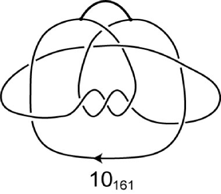
Figure 1. $10_{161}(0)$

It is not difficult to check that this knot is a $(1,1)$-knot in $S^{3}$. In fact, Figure $10_{161}(1)$ illustrates a $(1,1)$-decomposition $(V_{\alpha},t_{\alpha})\cup(V_{\beta},t_{\beta})$ of $(S^{3},K)$, and the shaded disc in the figure illustrates a meridian disc $D_{\alpha}^{2}$ of $V_{\alpha}$ which is disjoint from $C_{\alpha}$. Further Figures $10_{161}(2)-(5)$ show that the arc $t_{\beta}$ is trivial in $V_{\beta}$, and they also show a construction of a meridian disc $D_{\beta}^{2}$ of $V_{\beta}$ which is disjoint from $C_{\beta}$.

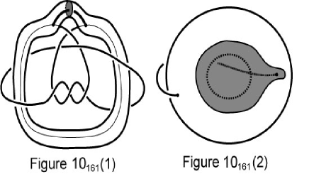
Figure 2.

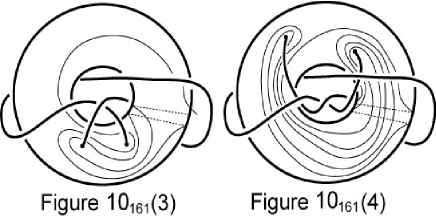
Figure 3.

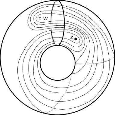
Figure 4. $10_{161}(5)$

A genus $2$ Heegaard splitting of $S^{3}$ constructed in Proposition 2.3 can be destabilized along $D_{\alpha}^{1}$ and $D_{\beta}^{1}$. In fact, Figure $10_{161}(5)$ illustrates a Heegaard diagram of genus 1 of $S^{3}$ which is obtained from that of genus 2 after the destabilization along $D_{\alpha}^{1}$ and $D_{\beta}^{1}$. On the Heegaard surface of genus 1 (which is a torus $\Sigma$), meridian curves $\partial D_{\alpha}^{2}$ and $\partial D_{\beta}^{2}$, and two reference points $w$ and $z$ are illustrated in Figure $10_{161}(5)$. Moreover, Figure $10_{161}(6)$ illustrates the corresponding diagram on the annulus which is obtained from the torus $\Sigma$ by cutting along $\partial D_{\alpha}^{2}$.

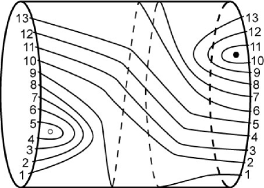
Figure 5. $10_{161}(6)$

Finally, Figure $10_{161}(7)$ illustrates the corresponding diagram of $\widetilde{\alpha}$ and $\widetilde{\beta}$ on the universal cover $\mathbb{C}$ of the torus $\Sigma$, where $\widetilde{\alpha}$ (resp. $\widetilde{\beta}$) is a lift of $\partial D_{\alpha}^{2}$ (resp. $\partial D_{\beta}^{2}$) in $\mathbb{C}$. Lightly-shaded (resp. darkly-shaded) circles represent lifts of the reference point $w$ (resp. $z$) in $\mathbb{C}$. The point labeled $\widetilde{x}$ on $\mathbb{C}$, which is an intersection point of $\widetilde{\alpha}$ and $\widetilde{\beta}$, is a lift of the point $x$ on the torus $\Sigma$.

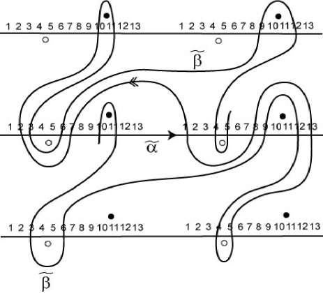
Figure 6. $10_{161}(7)$

Proposition 6.4 in [21] shows that if there exists a holomorphic disc in $\pi_{2}(\widetilde{x},\widetilde{y})$, then the absolute value of the coefficient of $\widetilde{y}$ in the expression of $\partial[\widetilde{x};i,j]$ is 1. In the following, we try to explain how to assign $+1$ or $-1$ to the coefficient of $\widetilde{y}$ in the expression of $\partial[\widetilde{x};i,j]$.

Let $u(x,y)$ denote a representative in $\mathbb{C}$ of a holomorphic disc in $\pi_{2}(\widetilde{x},\widetilde{y})$, where $\{\widetilde{x},\widetilde{y}\}\in\{\widetilde{x}_{1},\widetilde{x}_{2},\cdots,\widetilde{x}_{13}\}$. Note that every holomorphic disc in $\pi_{2}(\widetilde{x},\widetilde{y})$ can be represented as an embedded disc in the universal cover $\mathbb{C}$ of $\Sigma$. Then Figure $10_{161}(7)$ illustrates orientations of the curves $\widetilde{\alpha}$ and $\widetilde{\beta}$ which are given as totally real submanifolds of $\mathbb{C}$. Since the boundary of the disc $u(x,y)$ consists of a subarc of $\widetilde{\alpha}$ and a subarc of $\widetilde{\beta}$, this orientation of $\widetilde{\alpha}$ induces an orientation of the boundary of the disc $u(x,y)$, and an orientation of the disc $u(x,y)$.

Now hereafter, we also use the same notation as in $\S$3.6 of [17], but we use a connection over the universal cover $\mathbb{C}$ of ${\rm Sym}^{1}(\Sigma)=\Sigma$ which is trivial along $\widetilde{\alpha}$. Next we choose a contraction of the disc $\mathbb{D}$ to preserve the subarc of $\partial\mathbb{D}$ mapping into $\widetilde{\alpha}$. The linear transformation from ${\mathbb{C}}\cong{T_{u(0+i)}}\widetilde{\beta}\otimes_{\mathbb{R}}\mathbb{C}$ to $T_{u(0)}\widetilde{\beta}\otimes_{\mathbb{R}}\mathbb{C}\cong\mathbb{C}$ corresponds to a complex number $A(1)\in GL(1;\mathbb{C})=\mathbb{C}$. Then $A(1)$ induces an orientation of the disc $u(x,y)$. We assign a sign $\varepsilon(x,y)=+1$ (resp. $\varepsilon(x,y)=-1$) to the disc $u(x,y)$ if the above two orientations of the disc $u(x,y)$ agree (resp. disagree). These assignments $\varepsilon(x,y)$ give an orientation of 1-dimensional subspaces of the moduli space.

In order to choose a coherent orientation for all moduli spaces, we follow the arguments in $\S$21 of [5]. In this paragraph, we use the same notation as in $\S$21 of [5]. The above choice of an orientation for 1-dimensional subspaces of the moduli space gives an orientation for ${\rm Index}\,\bar{\partial}_{(u;\Lambda(x),\Lambda(y))}$. We choose the same orientation on ${\rm Index}\,\bar{\partial}_{(-,\Lambda(x))}$ for each $\widetilde{x}\in\widetilde{\alpha}\cap\widetilde{\beta}$, and we choose the same orientation on ${\rm Index}\,\bar{\partial}_{(+,\Lambda(y))}$ for each $\widetilde{y}\in\widetilde{\alpha}\cap\widetilde{\beta}$. Then we see from Remark 21.12 (2), Proposition 23.2 and Lemma 23.4 in [5] that these choices of orientations give a coherent orientation for all moduli spaces. Hence we obtain the following proposition.

Proposition 3.1.

Let $K$ be a $(1,1)$-knot in $S^{3}$. Suppose that the corresponding Heegaard diagram on $\mathbb{C}$ is constructed as above. Then the coefficient of the generator corresponding to the point $\widetilde{y}$ in the expression of $\partial[\widetilde{x};i,j]$ is equal to $\varepsilon(x,y)$.

For example, we assign $+1$ (resp. $-1$) to the coefficient of the generator corresponding to the point $\widetilde{x}_{1}$ in the expression of $\partial[\widetilde{x}_{7};i,j]$ (resp. $\partial[\widetilde{x}_{8};i,j]$). From Figure $10_{161}(7)$, we can verify that the complex $CFK^{\infty}(S^{3},K)$ is a $\mathbb{Z}$-module generated by

$$[\widetilde{x}_{1};i,i],\ [\widetilde{x}_{2};i-1,i+1],\ [\widetilde{x}_{3};i-1,i],\ [\widetilde{x}_{4};i,i-2],\ [\widetilde{x}_{5};i+1,i-2],$$

$$[\widetilde{x}_{6};i,i],\ [\widetilde{x}_{7};i,i+1],\ [\widetilde{x}_{8};i+1,i],\ [\widetilde{x}_{9};i,i],\ [\widetilde{x}_{10};i-2,i+1],$$

$$[\widetilde{x}_{11};i-2,i],\ [\widetilde{x}_{12};i,i-1]\ \mathrm{and}\ [\widetilde{x}_{13};i+1,i-1]$$

for $i\in\mathbb{Z}$, and the boundary operator on $CFK^{\infty}(S^{3},K)$ is explicitly given by

$$\partial[\widetilde{x}_{1};i,i] =[\widetilde{x}_{4};i,i-2]-[\widetilde{x}_{11};i-2,i],$$

$$\partial[\widetilde{x}_{2};i-1,i+1] =[\widetilde{x}_{3};i-1,i],$$

$$\partial[\widetilde{x}_{3};i-1,i] =0,$$

$$\partial[\widetilde{x}_{4};i,i-2] =0,$$

$$\partial[\widetilde{x}_{5};i+1,i-2] =-[\widetilde{x}_{4};i,i-2],$$

$$\partial[\widetilde{x}_{6};i,i] =[\widetilde{x}_{4};i,i-2]-[\widetilde{x}_{3};i-1,i],$$

$$\partial[\widetilde{x}_{7};i,i+1] =[\widetilde{x}_{1};i,i]-[\widetilde{x}_{2};i-1,i+1]-[\widetilde{x}_{6};i,i]+[\widetilde{x}_{10};i-2,i+1],$$

$$\partial[\widetilde{x}_{8};i+1,i] =[\widetilde{x}_{9};i,i]+[\widetilde{x}_{13};i+1,i-1]-[\widetilde{x}_{1};i,i]-[\widetilde{x}_{5};i+1,i-2],$$

$$\partial[\widetilde{x}_{9};i,i] =[\widetilde{x}_{12};i,i-1]-[\widetilde{x}_{11};i-2,i],$$

$$\partial[\widetilde{x}_{10};i-2,i+1] =[\widetilde{x}_{11};i-2,i],$$

$$\partial[\widetilde{x}_{11};i-2,i] =0,$$

$$\partial[\widetilde{x}_{12};i,i-1] =0,$$

$$\partial[\widetilde{x}_{13};i+1,i-1] =-[\widetilde{x}_{12};i,i-1].$$

The homology of the complex $CFK^{0,*}(S^{3},K)$ is ${\mathbb{Z}}\cong\widehat{HF}(S^{3})$, which is generated by the cycle $[\widetilde{x}_{5};0,-3]$. Its absolute grading is defined to be 0 (see [20]). We then obtain the knot Floer homology of the knot $10_{161}$ in $S^{3}$ as follows:

${\widehat{HFK}}(S^{3},10_{161},i)\cong\begin{cases}{{\mathbb{Z}}_{(6)}}&\text{$i=3$}\\ {{\mathbb{Z}}_{(4)}}\oplus{{\mathbb{Z}}_{(5)}}&\text{$i=2$}\\ {{\mathbb{Z}}_{(3)}^{2}}&\text{$i=1$}\\ {{\mathbb{Z}}_{(2)}^{3}}&\text{$i=0$}\\ {{\mathbb{Z}}_{(1)}^{2}}&\text{$i=-1$}\\ {{\mathbb{Z}}_{(0)}}\oplus{{\mathbb{Z}}_{(1)}}&\text{$i=-2$}\\ {{\mathbb{Z}}_{(0)}}&\text{$i=-3$}\\ 0&\text{otherwise.}\end{cases}$

Corollary 3.2.

The genus $g(K)$, the $4$-genus $g_{4}(K)$ and the unknotting number $u(K)$ of the knot $K=10_{161}$ are $3$.

Proof.

The adjunction inequality, Theorem 5.1 in [21], shows that $g(K)\geq 3$, and it is easy to see that $K$ bounds a Seifert surface of genus three. It follows that $g(K)=3$.

We next calculate the invariant $\tau(K)$, defined in [24]. The subcomplex ${\mathcal{F}}(K,-3)$ is generated by the generator corresponding to the point $\widetilde{x}_{5}$, and the homology $H_{*}({\mathcal{F}}(K,-3))$ is generated by the cycle corresponding to the point $\widetilde{x}_{5}$, whose absolute grading is 0. It follows that $\tau(K)=-3$. Corollary 1.3 in [24] shows $g_{4}(K)\geq|\tau(K)|=3$. Since $g(K)=3$, we have $g_{4}(K)\leq 3$ and hence $g_{4}(K)=3$. It is easy to see that crossing changes at three crossings change $K$ to the trivial knot. See, for example, [24] or [30]. It is well-known that $u(K)\geq g_{4}(K)$, so we have $u(K)=3$. ∎

Remark 3.3.

The 4-genus and the unknotting number of the knot $10_{161}$ were determined independently by Tanaka [30], Kawamura [9] and Ozsváth-Szabó [24].

4. Tunnel number 1 knots with 10 crossings

Tunnel number 1 knots up to ten crossings are determined in [14]. In this section, we present a list of the knot Floer homology of non-alternating $(1,1)$-knots with ten crossings.

Knot Floer homology of alternating knots is known to be described by using their signatures [22]. That of prime knots up to nine crossings are treated in [25]. We illustrate here tunnel number 1 knots up to ten crossings with $(1,1)$-tunnels except for these knots at the end of this paper. Note that the set of tunnel number 1 knots include that of $(1,1)$-knots, and that we can actually verify non-alternating tunnel number 1 knots with ten crossings have $(1,1)$-decompositions. We use here the notation in Rolfsen’s book [27].

Lemma 4.1.

Non-alternating $(1,1)$-knots with ten crossings are given in Figure $17$. Moreover $(1,1)$-tunnel of them are indicated by thick arcs in each figure.

Theorem 4.2.

Let $K=10_{n}$ be a non-alternating $(1,1)$-knot with ten crossings. Then the knot Floer homology of $K$ and the invariant $\tau(K)$ are given in Table $1$.

Table 1. $\widehat{HFK}(S^{3},10_{n},i)$

$n$	$\tau(K)$	$i=0$	$i=1$	$i=2$	$i=3$	$i=4$	$i\geq 5$
$124$	$4$	$\mathbb{Z}_{(-3)}$	$\mathbb{Z}_{(-2)}$	$0$	$\mathbb{Z}_{(-1)}$	$\mathbb{Z}_{(0)}$	$0$
$125$	$1$	$\mathbb{Z}_{(-1)}$	$\mathbb{Z}_{(0)}^{2}$	$\mathbb{Z}_{(1)}^{2}$	$\mathbb{Z}_{(2)}$	$0$	$0$
$126$	$-1$	$\mathbb{Z}_{(1)}^{5}$	$\mathbb{Z}_{(2)}^{4}$	$\mathbb{Z}_{(3)}^{2}$	$\mathbb{Z}_{(4)}$	$0$	$0$
$127$	$-2$	$\mathbb{Z}_{(2)}^{7}$	$\mathbb{Z}_{(3)}^{6}$	$\mathbb{Z}_{(4)}^{4}$	$\mathbb{Z}_{(5)}$	$0$	$0$
$128$	$3$	$\mathbb{Z}_{(-2)}$	$\mathbb{Z}_{(-2)}$	$\mathbb{Z}_{(-1)}^{3}$	$\mathbb{Z}_{(0)}^{2}$	$0$	$0$
$129$	$0$	$\mathbb{Z}_{(0)}^{9}$	$\mathbb{Z}_{(1)}^{6}$	$\mathbb{Z}_{(2)}^{2}$	$0$	$0$	$0$
$130$	$0$	$\mathbb{Z}_{(0)}^{5}$	$\mathbb{Z}_{(1)}^{4}$	$\mathbb{Z}_{(2)}^{2}$	$0$	$0$	$0$
$131$	$-1$	$\mathbb{Z}_{(1)}^{11}$	$\mathbb{Z}_{(2)}^{8}$	$\mathbb{Z}_{(3)}^{2}$	$0$	$0$	$0$
$132$	$-1$	$\mathbb{Z}_{(0)}^{2}\oplus\mathbb{Z}_{(1)}$	$\mathbb{Z}_{(1)}^{2}\oplus\mathbb{Z}_{(2)}$	$\mathbb{Z}_{(2)}$	$0$	$0$	$0$
$133$	$-1$	$\mathbb{Z}_{(1)}^{7}$	$\mathbb{Z}_{(2)}^{5}$	$\mathbb{Z}_{(3)}$	$0$	$0$	$0$
$134$	$3$	$\mathbb{Z}_{(-3)}^{3}$	$\mathbb{Z}_{(-2)}^{4}$	$\mathbb{Z}_{(-1)}^{4}$	$\mathbb{Z}_{(0)}^{2}$	$0$	$0$
$135$	$0$	$\mathbb{Z}_{(0)}^{13}$	$\mathbb{Z}_{(1)}^{9}$	$\mathbb{Z}_{(2)}^{3}$	$0$	$0$	$0$
$136$	$0$	$\mathbb{Z}_{(-1)}^{6}\oplus\mathbb{Z}_{(0)}$	$\mathbb{Z}_{(0)}^{4}$	$\mathbb{Z}_{(1)}$	$0$	$0$	$0$
$137$	$0$	$\mathbb{Z}_{(0)}^{11}$	$\mathbb{Z}_{(1)}^{6}$	$\mathbb{Z}_{(2)}$	$0$	$0$	$0$
$138$	$1$	$\mathbb{Z}_{(-1)}^{7}$	$\mathbb{Z}_{(0)}^{8}$	$\mathbb{Z}_{(1)}^{5}$	$\mathbb{Z}_{(2)}$	$0$	$0$
$139$	$4$	$\mathbb{Z}_{(-3)}^{3}$	$\mathbb{Z}_{(-2)}^{2}$	$0$	$\mathbb{Z}_{(-1)}$	$\mathbb{Z}_{(0)}$	$0$
$145$	$-2$	$\mathbb{Z}_{(1)}^{4}\oplus\mathbb{Z}_{(2)}$	$\mathbb{Z}_{(2)}^{2}\oplus\mathbb{Z}_{(3)}$	$\mathbb{Z}_{(4)}$	$0$	$0$	$0$
$161=162$	$-3$	$\mathbb{Z}_{(2)}^{3}$	$\mathbb{Z}_{(3)}^{2}$	$\mathbb{Z}_{(4)}\oplus\mathbb{Z}_{(5)}$	$\mathbb{Z}_{(6)}$	$0$	$0$

Remark 4.3.

As was stated in [21] Section 3, it holds that

$$\widehat{HFK}_{d}(S^{3},K,i)\cong\widehat{HFK}_{d-2i}(S^{3},K,-i).$$

Thereby we have given a list of $\widehat{HFK}(S^{3},K,i)$ only for $i\geq 0$.

Proof.

We can directly apply the method discussed in Section 3 to these $(1,1)$-knots. However the calculation is straightforward and lengthy, so that we omit here. ∎

Example 4.4.

Let us consider the knot $K_{1}=8_{8}$, which is an alternating $(1,1)$-knot. It has the Alexander polynomial $9-6(t+t^{-1})+2(t^{2}+t^{-2})$ and the signature zero. Thus we have $\widehat{HFK}(S^{3},K_{1},i)=\mathbb{Z}_{(i)}^{|a_{i}|}$, where $a_{i}$ denotes the coefficient of $i$-th term of the Alexander polynomial (see [22]). Further, $\tau(K_{1})=0$ from Theorem 1.4 in [24]. We then see from Theorem 4.2 that the knot Floer homology and $\tau$ of $K_{2}=10_{129}$ are same as those of $K_{1}$. Further, it is known that these two knots have the same Alexander polynomial and Jone polynomial, but are not mutant each other [12]. M. Teragaito informed us this example.

5. Pretzel knots

Tunnel number 1 pretzel knots are determined in [11] and [14]. More precisely, the type is $(\pm 2,m,n)$, where $m$ and $n$ are odd integers. It is not difficult to check that all of them admit $(1,1)$-decompositions. In this section, we show the following theorem. See [10] as for the classification of pretzel knots. In particular, we remark here that $P(\pm 2,m,n)$ is equivalent to $P(\pm 2,n,m)$.

Theorem 5.1.

Let $K$ be the pretzel knot $P(-2,m,n)$, where $m$ and $n$ are odd integers satisfying $m\geq n\geq 3$. Then we have

${\widehat{HFK}}(S^{3},K,i)\ \cong\ \begin{cases}0&\text{$(i>g)$}\\ {\mathbb{Z}}_{(g+i)}&\text{$(i=g,\ g-1)$}\\ 0&\text{$(i=g-2)$}\\ {\mathbb{Z}}^{g-2-i}_{(g-1+i)}&\text{$(g-n\leq i<g-2)$}\\ {\mathbb{Z}}^{n-2}_{(g-1+i)}&\text{$(0\leq i<g-n)$}\end{cases}$

where $\displaystyle{g=\frac{m+n}{2}}$ denotes the genus of the pretzel knot $K$. Moreover, the invariant $\tau(K)$ is $-g$.

Remark 5.2.

Knot Floer homology of the remaining tunnel number 1 pretzel knots can be calculated by the same method as in stated below.

Corollary 5.3.

The $4$-genus $g_{4}(K)$ and the unknotting number $u(K)$ of the pretzel knot $K=P(-2,m,n)$ are equal to the genus $\displaystyle{g=\frac{m+n}{2}}$.

Proof.

It is clear that the invariant $\tau(K)$ is equal to $-g$. Thereby the claim follows from the same argument in the proof of Corollary 3.2. ∎

At first, we present how to construct a genus $1$ Heegaard diagram for pretzel knots with $(1,1)$-decompositions.

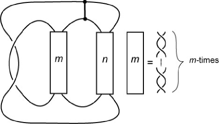
Figure 7.

The pretzel knots of type $(-2,m,n)$ have projection as illustrated in Figure 7. All of them have a $(1,1)$-tunnel, for example, we present a $(1,1)$-tunnel there. Pretzel knots of this type have the $(1,1)$-tunnel in the same position. Let $T$ be the unknotted torus as in Figure 8, and we denote by $V_{1}$ (resp. $V_{2}$) the solid torus $D^{2}\times S^{1}$ which is bounded ‘inside’ (resp. ‘outside’) by $T$. We can see that $(V_{1},k_{1})$ forms the pair of a solid torus and a trivial arc. We can also observe that $(V_{2},k_{2})$ is the pair of them by an isotopy, which we call $P$-isotopy.

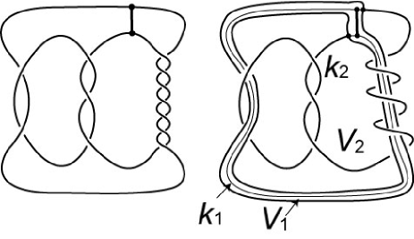
Figure 8.

In what follows, we consider the inverse of $P$-isotopy.

We can find a meridian disk $D_{2}$ in $V_{2}$ as in Figure 9. We do proper isotopy for $k_{2}$ to make $k$ an ‘almost’ pretzel knot. Here, since we need the information on $\mbox{$\partial$}D_{2}$, we trace only $\mbox{$\partial$}D_{2}$ under the inverse of $P$-isotopy.

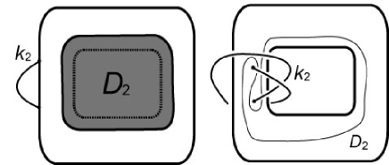
Figure 9.

For the pretzel knot $P(-2,m,n)$, we restore the part of ‘$-2$’ and ‘$m$’ part as illustrated in Figures 9 and 10. Continuing this way, we have the train track as in the left-hand of Figure 11.

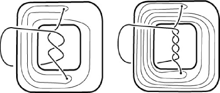
Figure 10.

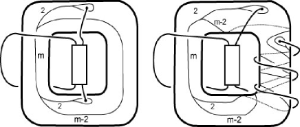
Figure 11.

In order to restore the ‘$n$’ part, we do the remaining of the inverse of $P$-isotopy as in right-hand of Figure 11. Accordingly, we obtain a Heegaard diagram of the pretzel knot of type $(-2,m,n)$. For example, a Heegaard diagram of the pretzel knot $P(-2,m,7)$ is illustrated in Figure 12.

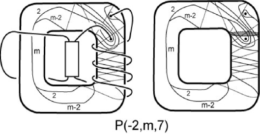
Figure 12.

Therefore we have

Lemma 5.4.

A Heegaard diagram for the pretzel knot $P(-2,m,n)$, where $m$ and $n$ are positive odd integers greater than one, is carried by the train track as illustrated in Figure $13$.

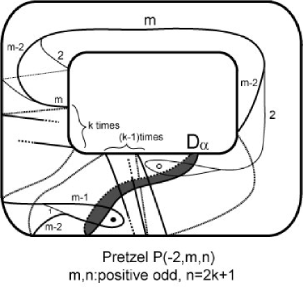
Figure 13.

In order to treat uniformly, we assume $m\geq n\geq 5$ in the following. After reading the proof for this, one can calculate the knot Floer homology of the pretzel knots of type $(-2,m,3)$ by the same method.

By the straightforward calculation and taking a proper framing, we have

Lemma 5.5.

Suppose $n\geq 5$. Figure $14$ illustrates the diagram of $\widetilde{\alpha}$ and $\widetilde{\beta}$ on the universal cover $\mathbb{C}$ of the torus $\Sigma$ for the pretzel knot $P(-2,m,n)$, where $\widetilde{\alpha}$ $($resp. $\widetilde{\beta})$ is a lift of $\partial D_{\alpha}^{2}$ $($resp. $\partial D_{\beta}^{2})$ in $\mathbb{C}$.

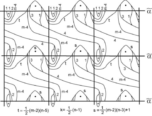
Figure 14.

Next we explicitly give the boundary operator from the Heegaard diagram constructed above. We use the following notations. There is a holomorphic disc $\mathbb{D}_{1}$ (resp. $\mathbb{D}_{2}$) such that it is bounded by an subarc in $\widetilde{\mbox{$\alpha$}}$ and that of $\widetilde{\mbox{$\beta$}}$, ${\rm int}\mathbb{D}_{1}\cap(\widetilde{\mbox{$\alpha$}}\cup\widetilde{\mbox{$\beta$}})=\emptyset$ (resp. ${\rm int}\mathbb{D}_{2}\cap(\widetilde{\mbox{$\alpha$}}\cup\widetilde{\mbox{$\beta$}})=\emptyset$), and $\mathbb{D}_{1}$ (resp. $\mathbb{D}_{2}$) contains darkly-shaded (resp. lightly-shaded) point. We denote $\widetilde{\mbox{$\alpha$}}\cap\widetilde{\mbox{$\beta$}}\cap\mbox{$\partial$}\mathbb{D}_{1}$ by $\widetilde{y}_{1}$ and $\widetilde{y}_{2}$ from the left hand side. Similarly, let denote $\widetilde{\mbox{$\alpha$}}\cap\widetilde{\mbox{$\beta$}}\cap\mbox{$\partial$}\mathbb{D}_{2}$ by $\widetilde{y}_{3}$ and $\widetilde{y}_{4}$. We call $\widetilde{y}_{1},\widetilde{y}_{2},\widetilde{y}_{3},\widetilde{y}_{4}$ exceptional generators (see Figure 15). Focus on $(m-2)$-lines of $\widetilde{\mbox{$\beta$}}$ just the right hand side of $\widetilde{y}_{4}$. Toward left hand side, these lines run parallel until they intersect $(n-2)$ times with $\widetilde{\alpha}$. We call these parallel lines a bunch of $(m-2)$-lines, and call $1$-stage, $2$-stage,$\ldots$, $(n-2)$-stage from the left hand side at each part of the intersection of $\widetilde{\alpha}$ and the bunch of $(m-2)$-lines. Thus each stage has $(m-2)$ points of $\widetilde{\alpha}\cap\widetilde{\beta}$, so we name $\widetilde{x}_{i,1},\widetilde{x}_{i,2},\ldots,\widetilde{x}_{i,m-2}$ from the left hand side to the right hand side at the $i$-stage (see Figure 16).

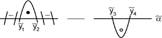
Figure 15.

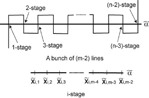
Figure 16.

Then, by direct calculations as in Section 3, we see that $CFK^{\infty}\left(S^{3},P(-2,m,n)\right)$ is generated as a $\mathbb{Z}$-module by generators indexed by $i\in\mathbb{Z}$ of the form:

$$[\widetilde{y}_{1};i+\gamma(g)-1,i+\delta(g)+1],\quad[\widetilde{y}_{2};i+\gamma(g)-1,i+\delta(g)],$$

$$[\widetilde{y}_{3};i+\delta(g),i+\gamma(g)-1],\quad[\widetilde{y}_{4};i+\delta(g)+1,i+\gamma(g)-1],$$

$$[\widetilde{x}_{2p+1,2q+1};i+\gamma(g)+p+q+1,i+\delta(g)-p-q]\quad\left(0\leq p\leq n^{\prime},\ 0\leq q\leq m^{\prime}\right),$$

$$[\widetilde{x}_{2p+1,2q};i+\gamma(g)+p+q,i+\delta(g)-p-q]\quad\left(0\leq p\leq n^{\prime},\ 1\leq q\leq m^{\prime}\right),$$

$$[\widetilde{x}_{2p,2q+1};i+\gamma(g)+m^{\prime}+p-q,i+\delta(g)-m^{\prime}-p+q]\quad\left(1\leq p\leq n^{\prime},\ 0\leq q\leq m^{\prime}\right),$$

$$[\widetilde{x}_{2p,2q};i+\gamma(g)+m^{\prime}+p-q,i+\delta(g)-m^{\prime}-p+q-1]\quad\left(1\leq p\leq n^{\prime},\ 1\leq q\leq m^{\prime}\right)$$

where $\displaystyle{g=\frac{m+n}{2},\ m^{\prime}=\frac{m-3}{2},\ n^{\prime}=\frac{n-3}{2}}$ and

$$\gamma(g)=\left\{\begin{gathered}1-\frac{g-1}{2}\quad(g:\mathrm{odd})\\ 1-\frac{g}{2}\ \qquad(g:\mathrm{even})\end{gathered}\right.\qquad\delta(g)=\left\{\begin{gathered}\frac{g-1}{2}\qquad(g:\mathrm{odd})\\ \frac{g}{2}-1\qquad(g:\mathrm{even}).\end{gathered}\right.$$

Then the boundary operator on $CFK^{\infty}\left(S^{3},P(-2,m,n)\right)$ is explicitly given by the following lemmas.

Lemma 5.6.

For exceptional generators: $\widetilde{y}_{1},\widetilde{y}_{2},\widetilde{y}_{3},\widetilde{y}_{4}$, we have

$\partial[\widetilde{y}_{1};i,j]=[\widetilde{y}_{2};i,j-1],$

$\partial[\widetilde{y}_{2};i,j]=0$,

$\partial[\widetilde{y}_{3};i,j]=0$,

$\partial[\widetilde{y}_{4};i,j]=-[\widetilde{y}_{3};i-1,j]$.

Lemma 5.7.

For generators $\widetilde{x}_{1,q}\ (1\leq q\leq m-2)$, we have

$\partial[\widetilde{x}_{1,1};i,j]=[\widetilde{x}_{2,m-2};i,j-1]+[\widetilde{x}_{1,2};i,j-1]-[\widetilde{y}_{2};i-2,j]$,

$\partial[\widetilde{x}_{1,2l};i,j]=[\widetilde{x}_{2,m-2l-1};i,j-1]\quad\left(1\leq l\leq m^{\prime}\right)$,

$\partial[\widetilde{x}_{1,2l+1};i,j]=[\widetilde{x}_{2,m-2l-2};i,j-1]+[\widetilde{x}_{1,2l+2};i,j-1]-[\widetilde{x}_{1,2l};i-1,j]\quad\left(1\leq l\leq m^{\prime}-1\right)$,

$\partial[\widetilde{x}_{1,m-2};i,j]=[\widetilde{x}_{2,1};i,j-1]-[\widetilde{x}_{1,m-3};i-1,j]$.

Lemma 5.8.

For generators $\widetilde{x}_{n-2,q}\ (1\leq q\leq m-2)$, we have

$\partial[\widetilde{x}_{n-2,1};i,j]=[\widetilde{x}_{n-2,2};i,j-1]-[\widetilde{x}_{n-3,m-2};i-1,j]$,

$\partial[\widetilde{x}_{n-2,2l};i,j]=-[\widetilde{x}_{n-3,m-2l-1};i-1,j]\quad\left(1\leq l\leq m^{\prime}\right)$,

$\partial[\widetilde{x}_{n-2,2l+1};i,j]=-[\widetilde{x}_{n-3,m-2l-2};i-1,j]-[\widetilde{x}_{n-2,2l};i-1,j]$

$\qquad\qquad\qquad\qquad+[\widetilde{x}_{n-2,2l+2};i,j-1]\quad\left(1\leq l\leq m^{\prime}-1\right)$,

$\partial[\widetilde{x}_{n-2,m-2};i,j]=-[\widetilde{x}_{n-3,1};i-1,j]-[\widetilde{x}_{n-2,m-3};i-1,j]+[\widetilde{y}_{3};i,j-2]$.

Lemma 5.9.

For generators $\widetilde{x}_{2k,q}\ (1\leq k\leq n^{\prime})$, we have

$\partial[\widetilde{x}_{2k,1};i,j]=[\widetilde{x}_{2k,2};i-1,j]$,

$\partial[\widetilde{x}_{2k,2l};i,j]=0\quad\left(1\leq l\leq m^{\prime}\right)$,

$\partial[\widetilde{x}_{2k,2l+1};i,j]=[\widetilde{x}_{2k,2l+2};i-1,j]-[\widetilde{x}_{2k,2l};i,j-1]\quad\left(1\leq l\leq m^{\prime}-1\right)$,

$\partial[\widetilde{x}_{2k,m-2};i,j]=-[\widetilde{x}_{2k,m-3};i,j-1]$.

Lemma 5.10.

For generators $\widetilde{x}_{2k+1,q}\ (1\leq k\leq n^{\prime}-1)$, we have

$\partial[\widetilde{x}_{2k+1,1};i,j]=[\widetilde{x}_{2k+2,m-2};i,j-1]+[\widetilde{x}_{2k+1,2};i,j-1]-[\widetilde{x}_{2k,m-2};i-1,j]$,

$\partial[\widetilde{x}_{2k+1,2l};i,j]=[\widetilde{x}_{2k+2,m-2l-1};i,j-1]-[\widetilde{x}_{2k,m-2l-1};i-1,j]\quad\left(1\leq l\leq m^{\prime}\right)$,

$\partial[\widetilde{x}_{2k+1,2l+1};i,j]=[\widetilde{x}_{2k+2,m-2l-2};i,j-1]+[\widetilde{x}_{2k+1,2l+2};i,j-1]$

$\qquad\qquad\qquad\quad-[\widetilde{x}_{2k,m-2l-2};i-1,j]-[\widetilde{x}_{2k+1,2l};i-1,j]\quad\left(1\leq l\leq m^{\prime}-1\right)$,

$\partial[\widetilde{x}_{2k+1,m-2};i,j]=[\widetilde{x}_{2k+2,1};i,j-1]-[\widetilde{x}_{2k+1,m-3};i-1,j]-[\widetilde{x}_{2k,1};i-1,j]$.

By using these lemmas, we can immediately obtain Theorem 5.1. In particular, we easily see that the Floer homology class of $\widehat{HF}(S^{3})\cong\mathbb{Z}$ is represented by the generator $[\widetilde{y}_{4};0,-g]$ (so its absolute grading is zero). Accordingly, we can also conclude that the invariant $\tau(P(-2,m,n))$ is equal to $-g$.

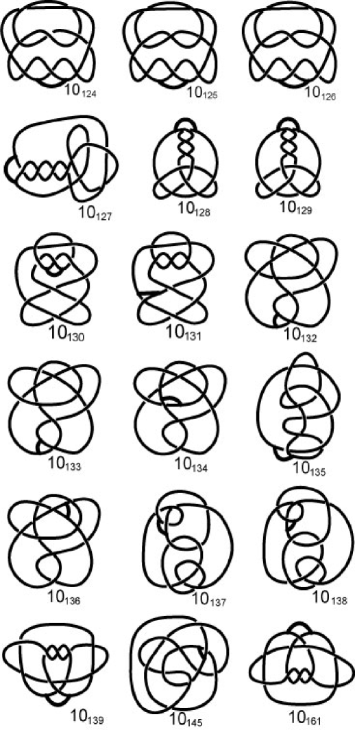
Figure 17.

References

- [1] J. Berge, Some knots with surgeries yielding lens spaces, unpublished manuscript.
- [2] A. Cattabriga, M. Mulazzani, -knots via the mapping class groups of the twice punctured torus, preprint, available at http://xxx.lanl.gov/math.GT/0205138.
- [3] D. H. Choi, K. H. Ko, Parameterization of -bridge torus knots, J. Knot Theory Ramification 12 (2003), 463–491.
- [4] H. Doll, A generalized bridge number for links in -manifolds, Math. Ann. 294 (1992), 701–717.
- [5] K. Fukaya, Y.-G. Oh, H. Ohta, K. Ono, Lagrangian intersection Floer theory -anomary and obstruction-, preprint, available at http://www.kusm.kyoto-u.ac.jp/ fukaya/fooo.dvi
- [6] H. Goda, C. Hayashi, Genus two Heegaard splittings of exteriors of -genus -bridge knots, preprint.
- [7] H. Goda, C. Hayashi, H. J. Song, A criterion for satellite -genus -bridge knots, to appear in Proc. Amer. Math. Soc.
- [8] C. Hayashi, Genus one -bridge positions for the trivial knot and cable knots, Math. Proc. Cambridge Philos. Soc. 125 (1999), 53–65.
- [9] T. Kawamura, The unknotting numbers of and are , Osaka J. Math. 35 (1998), 539–546.
- [10] A. Kawauchi, Classification of pretzel knots, Kobe J. Math. 2 (1985), 11–22.
- [11] E. Klimenko, M. Sakuma, Two-generator discrete subgroups of containing orientation-reversing elements, Geom. Dedicata 72 (1998), 247–282.
- [12] W. Lickorish, K. Millett, A polynomial invariant of oriented links, Topology 26 (1987), 107–141.
- [13] H. Matsuda, Genus one knots which admit -decompositions, Proc. Amer. Math. Soc. 130 (2002), 2155–2163.
- [14] K. Morimoto, M. Sakuma, Y. Yokota, Identifying tunnel number one knots, J. Math. Soc. Japan 48 (1996), 667–688.
- [15] M. Mulazzani, Cyclic presentations of groups and cyclic branched coverings of -knots, Bull. Korean Math. Soc. 40 (2003), no. 1, 101–108.
- [16] M. Eudave-Munoz, -knots and incompressible surfaces, preprint, available at http://www.lanl.arxiv.org/abs/math.GT/0201121.
- [17] P. Ozsváth, Z. Szabó, Holomorphic disks and topological invariants for closed three-manifolds, to appear in Ann. Math.
- [18] P. Ozsváth, Z. Szabó, Holomorphic disks and three-manifold invariants: properties and applications, to appear in Ann. Math.
- [19] P. Ozsváth, Z. Szabó, On the Floer homology of plumbed three-manifolds, Geom. Topol. 7 (2003), 185–224.
- [20] P. Ozsváth, Z. Szabó, Holomorphic triangles and invariants for smooth four-manifolds, preprint, available at http://xxx.lanl.gov/math.SG/0110169.
- [21] P. Ozsváth, Z. Szabó, Holomorphic disks and knot invariants, to appear in Adv. Math.
- [22] P. Ozsváth, Z. Szabó, Heegaard Floer homology and alternating knots, Geom. Topol. 7 (2003), 225–254.
- [23] P. Ozsváth, Z. Szabó, Heegaard Floer homologies and contact structures, preprint, available at http://xxx.lanl.gov/math.SG/0210127.
- [24] P. Ozsváth, Z. Szabó, Knot Floer homology and the four-ball genus, Geom. Topol. 7 (2003), 615-639.
- [25] P. Ozsváth, Z. Szabó, Knot Floer homology, genus bounds, and mutation, preprint, available at http://xxx.lanl.gov/math.GT/0303225.
- [26] J. Rasmussen, Floer homology of surgeries on two-bridge knots, Algebr. Geom. Topol. 2 (2002), 757–789.
- [27] D. Rolfsen, Knots and Links, Publish or Perish Inc.
- [28] T. Saito, Genus one -bridge knot as viewed from the curve complex, master’s thesis at Osaka University (2001).
- [29] M. Scharlemann, There are no unexpected tunnel number one knots of genus one, to appear in Trans. Amer. Math. Soc.
- [30] T. Tanaka, Unknotting numbers of quasipositive knots, Topology Appl. 88 (1998), 239–246.