Two Gauss-Bonnet and Poincaré-Hopf Theorems for Orbifolds with Boundary
Abstract
\OnePageChapterThe goal of this work is to generalize the Gauss-Bonnet and Poincaré-Hopf Theorems to the case of orbifolds with boundary. We present two such generalizations, the first in the spirit of [20], which uses an argument parallel to that contained in [22]. In this case, the local data (i.e. integral of the curvature in the case of the Gauss-Bonnet Theorem and the index of the vector field in the case of the Poincaré-Hopf Theorem) is related to Satake’s orbifold Euler characteristic, a rational number which depends on the orbifold structure.
For the second pair of generalizations, we use a more recent orbifold cohomology [3] to express the local data in a way which can be related to the Euler characteristic of the underlying space of the orbifold. This case applies only to orbifolds which admit almost-complex structures.
Seaton \otherdegreesB.A., Kalamazoo College, 1999 \degreeDoctor of Philosophy Ph.D., Mathematics \deptDepartment of Mathematics \advisorAssoc. Prof. Carla Farsi \readerSiye Wu \dedication[Dedication] To Michael Thomas Seaton and Christina Heather Bost, my siblings old and new, with congratulations and best wishes.
Acknowledgements.
\OnePageChapterI am honored to take this opportunity to thank my advisor, Carla Farsi, for her encouragement, instruction, and inspiration throughout my time at Colorado. This work would not have been possible without her. I would also like to thank Alexander Gorokhovsky, Erich McAlister, Arlan Ramsay, Yongbin Ruan, and Siye Wu for many helpful discussions and suggestions, and John Massman for helpful discussions and pointers about using LaTeX. As well, thanks to Lynne Walling for encouragement. Thanks are also due to the kids who would answer the phone at crazy hours of the night to listen to my frustration. To L.J., Demangy, Andrea, Crickey, Her Majesty, and my brother, thank you for your faith, support, and patience. And of course I would like to thank my parents for making everything possible. \ToCisShort\LoFisShort\emptyLoTChapter 1 Introduction
An orbifold is perhaps the simplest case of a singular space; it is a topological space which is locally diffeomorphic to where is a finite group. Orbifolds were originally introduced by Satake in [19] and [20], where they were given the name -manifold, and rediscovered by Thurston in [24], where the term orbifold was coined. Satake and Thurston’s definitions differ, however, in that Satake required the group action to have a fixed point set of codimension at least two, while Thurston did not. Hence, Thurston’s definition allows group actions such as reflections through hyperplanes. Today, authors differ on whether or not this requirement is made; often, when it is, the orbifolds are referred to as codimension-2 orbifolds. It is these orbifolds which are our object of study.
The point of view of this work is that an orbifold structure is a generalization of a differentiable structure on a manifold. We do not mean to suggest that the underlying space of an orbifold is necessarily a topological manifold; this is only the case in dimension , and not even in dimension 1 if the codimension-2 requirement is lifted. However, there are many examples of orbifolds whose underlying topological spaces are indeed manifolds. In these cases, we view the orbifold structure as a singular differentiable structure on the manifold. It should be noted that this is used as a guiding principle only, and that our results apply in general.
Hence, we improve upon Satake’s Gauss-Bonnet theorem for orbifolds [20] by developing a Gauss-Bonnet integrand (and corresponding orbifold Euler Class) whose integral relates to the Euler Characteristic of the underlying topological space, as opposed to the orbifold Euler Characteristic (Theorem 4.4.2). This result depends on recent developments in the theory of orbifolds, most notably the Orbifold Cohomology Theory of Chen-Ruan [3], and hence is restricted to the case of an orbifold which admits an almost complex structure.
As is well-known, the Gauss-Bonnet theorem is very closely related to the Poincaré-Hopf theorem; indeed, either of the two theorems can be viewed as a corollary of the other. With a new Gauss-Bonnet theorem, then, comes a new Poincaré-Hopf theorem. Following the work of Sha on the secondary Chern-Euler class for manifolds [22], we generalize the Poincaré-Hopf theorem to the case of orbifolds with boundary (Corollary 4.4.4).
To this end, a remark is in order. Satake’s original definition of an orbifold with boundary was in many senses not very strict. In particular, the boundaries of his orbifolds were not necessarily orbifolds. This allows little control over vector fields on the boundary; indeed, it is not generally the case that the orbifold is locally a product near the boundary, and hence there need not exist a vector field which does not vanish on the boundary. Since then, a more natural definition of orbifold with boundary has been given in [24]. Using this definition, we are able to refine Satake’s original Gauss-Bonnet theorem for the case with boundary using his original techniques.
The outline of this work is roughly as follows. In Chapter 2, we collect the necessary background information on orbifolds and orbifolds with boundary, including several examples, paying particular attention to the behavior of vector fields on orbifolds. In Chapter 3, we review Satake’s Gauss-Bonnet and Poincaré-Hopf theorems for orbifolds and orbifolds with boundary, making improvements where possible using the modern definition of an orbifold with boundary (see Theorem 3.2.2). We also apply the arguments of Sha [22] to characterize the boundary term in the case with boundary as the evaluation of a secondary characteristic class on the boundary (see Theorem 3.4.2). It is easy to see that, even in the case of a manifold, the boundary term of this formula will always depend on the vector field. For instance, consider a fixed vector field on with one singular point . Remove an open disk to produce a vector field on a manifold with boundary. The index of the vector field depends on whether is contained in the disk removed, but the Euler Characteristic does not; hence, the boundary term must depend on the vector field. The spirit of the Poincaré-Hopf theorem is that this term should be formulated in a manner as independent of the vector field as possible; it is this reason that we chose the result of Sha to generalize to orbifolds.
In Chapter 4, we review the Chen-Ruan orbifold cohomology, and extend it in a straightforward manner to the case with boundary. Loosely speaking, the idea of this cohomology theory is to associate to an orbifold another orbifold, (where at least one of the connected components of is diffeomorphic to ), and use the cohomology groups of (we should note that this informal description leaves out an important modification to the grading of the groups). Using this cohomology theory, we develop an Euler Class which relates to the Euler Characteristic of the underlying topological space of . The essential idea here is to apply the Chern-Weil description of characteristic classes to the curvature of a connection on , yielding a (non-homogeneous) characteristic class in orbifold cohomology. Similarly, the index of a vector field on is computed to be the index of its pull-back onto . This suggests the paradigm that geometric structures on can be considered to be structures on which take multiple values on singular sets. It is in this manner that we prove the aforementioned Gauss-Bonnet and Poincaré-Hopf theorems for orbifolds (Theorem 4.4.2 and Corollary 4.4.4) and orbifolds with boundary (Theorems 4.5.1 and 4.5.2), relating to the Euler Characteristics of the underlying space.
Theorems, definitions, examples, etc. are numbered sequentially according to the section in which they appear. So Theorem is in Chapter , Section , and follows Definition (or Lemma, Example, etc.) . Figures are numbered independently according to the Chapter in which they appear.
Chapter 2 Orbifolds and Their Structure
2.1 Definitions and Examples
In this section, we collect the definitions and background we will need. For more information, the reader is referred to the original work of Satake in [19] and [20]. As well, [17] contains as an appendix a thorough introduction to orbifolds, focusing on their differential geometry. Other good introductions include [24] and [2], the former providing a great deal of information on the topology of low-dimensional orbifolds. The reader is warned that the definition used in these latter two works is more general than ours, as it admits group actions which fix sets of codimension 1. For the most part, we follow the spirit of Satake and Ruan.
2.1.1 Orbifolds and Orbifolds With Boundary
Let be a Hausdorff space.
Definition 2.1.1 (orbifold chart)
Let be a connected open set. A () orbifold chart for (also known as a () local unifomizing system) is a triple where
-
•
is an open subset of ,
-
•
is a finite group with a () action on such that the fixed point set of any which does not act trivially on has codimension at least 2 in , and
-
•
is a surjective continuous map such that , that induces a homeomorphism .
If acts effectively on , then the chart is said to be reduced.
The definition of the appropriate notion of ‘chart’ for orbifolds with boundary is similar:
Definition 2.1.2 (orbifold chart with boundary)
Let be a connected open set. A () orbifold chart with boundary or () local unifomizing system for is a triple where
-
•
is an open subset of ,
-
•
is a finite group with a () action on such that the fixed point set of any which does not act trivially on has codimension at least 2 in , and such that , and
-
•
is a surjective continuous map such that , that induces a homeomorphism .
Again, if acts effectively on , then the chart is said to be reduced.
If , then is an ordinary orbifold chart; for emphasis, we may refer to these as orbifold charts without boundary. Note also that if is an orbifold chart with boundary for some set , then restricting the chart to , it is clear that is an orbifold chart without boundary for .
We will always use the notation that if is the domain of a chart, then is the group of the chart, the projection for the chart, and the range of the chart; i.e. items with the same subscript correspond to the same chart.
Orbifold charts relate to one another via injections.
Definition 2.1.3 (injection)
If and are two orbifold charts (with or without boundary) for and , respectively, where , then an injection is a pair where
-
•
is an injective homomorphism such that if and denote the kernel of the action of and , respectively, then restricts to an isomorphism of onto , and
-
•
is a smooth embedding such that and such that for each , . If the charts have boundary then .
Given an orbifold chart (with or without boundary), each induces an injection of into itself via
Note that this injection is trivial if acts trivially. Similarly, given an injection , each element defines an injection with . Moreover, every two injections of into are related in this manner (see [20], Lemma 1).
Two orbifold charts and are said to be equivalent if , and there is an injection with an isomorphism and a diffeomorphism.
Definition 2.1.4 (orbifold)
An orbifold is a Hausdorff space , the underlying space of , together with a family of orbifold charts (without boundary) such that
-
•
Each is contained in an open set covered by an orbifold chart . If for and uniformized sets, then there is a uniformized set such that .
-
•
Whenever for two uniformized sets, there is an injection .
If each chart in is reduced, then is said to be a reduced orbifold. Otherwise, is unreduced.
The definition of an orbifold with boundary is identical, except that it allows orbifold charts with boundary. In this case, is the boundary of . It is easy to see that the restrictions endow with the structure of an orbifold. We will sometimes refer to an orbifold as an orbifold without boundary for emphasis.
It is easy to see that, given an unreduced orbifold , one can associate to it a reduced orbifold by redefining the group in each chart to be , where again denotes the kernel of the -action on .
Fix , and say for some set uniformized by . Let such that , and let denote the isotropy subgroup of . The isomorphism class of depends only on ; indeed, if is another choice of a lift, then there is a group element such that , so that and are conjugate via . Similary, if is another choice of chart with (and we assume, by shrinking domains if necessary, that ), then there is an injection with associated homomorphism that maps isomorphically onto (see [20], page 468). We will often refer to the (isomorphism class) of this group as the isotropy group of , denoted . If (with respect to the orbifold structure of in the case that is not reduced), then is singular; otherwise, it is nonsingular. The collection of singular points of is denoted .
2.1.2 Examples
Before proceeding, we give some examples of orbifolds.
Example 2.1.5
If is a smooth manifold and a group that acts properly discontinuously on such that the fixed point set of each element of has codimension , then the quotient is an orbifold ([20], [24]).
Similarly, we have the following claim.
Claim 2.1.6
If is a manifold with boundary and a group with action as above that fixes the boundary, then is an orbifold with boundary.
This is proven as follows, following Thurston’s proof ([24]) for the case of manifolds without boundary.
Let , and let project to . Note that, by hypothesis, if , then any point projecting to is also an element of . Hence, we may define to be the set of points which are projections of points in .
Now, in the case that is not an element of , we may use Thurston’s proof (by intersecting the neighborhood of with the interior of ) to produce a chart near . If , then let denote the isotropy group of . There is a neighborhood of invariant by and disjoint from its translates by elements of not in . Note that is diffeomorphic to a neighborhood of , where is the dimension of , and that is clearly -invariant. The projection is by fiat a homeomorphism.
To obtain a suitable cover of , augment some cover by adjoining finite intersections. Whenever , this means some set of translates has a corresponding non-empty intesection. This intersection may be taken to be with associated group .
With this, we need only note that Thurston’s proof (applied to the boundary, and restricted to ) will give a cover of , consistent with that on , making an orbifold. This completes the proof.
Orbifolds which arise in this way are called global quotient orbifolds or global quotients. They are examples of good orbifolds, orbifolds whose universal cover is a manifold or, equivalently, orbifolds diffeomorphic to the quotient of a manifold by the proper action of a discrete group. Orbifolds which are not good are called bad orbifolds.
Example 2.1.7
(Kawasaki [9]) If is a Lie group that acts smoothly on a smooth manifold such that
-
•
, the isotropy subgroup is compact,
-
•
, there is a smooth slice at ,
-
•
such that , there are slices and with , and
-
•
the dimension of is constant on ,
then is an orbifold. Moreover, every -dimensional orbifold can be expressed in this manner with the orthonormal frame bundle of and .
Example 2.1.8
The simplest example of an orbifold is that of a point with the trivial action of a finite group . Note that these orbifolds are not reduced unless .
Example 2.1.9
The -teardrop is a well-known example of a bad orbifold, whose underlying topological space is . It has one singular point, covered by a chart where is an open disk in about the origin on which acts via rotations, and every other point is covered by a chart with the trivial group (see Figure 2.1)).
In fact, every compact 2-dimensional orbifold (with or without boundary) can be constructed from a compact 2-dimensional manifold by removing disks and replacing them with for some finite cyclic group with one singular point. Note that in dimension 2, the boundary of the orbifold cannot contain singular points.
The underlying space of an orbifold need not be a topological manifold, even in dimensions 3, as is demonstrated by the following example (taken from [23]).
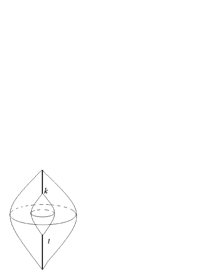
Example 2.1.10
Let act on via the antipodal map, and then the origin is the only fixed point. Then is clearly an orbifold with one singular point, yet its underlying space is homeomorphic to a cone on , which is not a manifold.
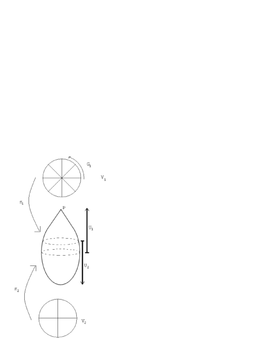
Example 2.1.11 (The --Solid Hollow Football)
An example of a bad orbifold with boundary is the --solid hollow football with . It is homeomorphic to the manifold with boundary with two boundary components, both homeomorphic to . Its orbifold structure, however, is such that both of the boundary components have the orbifold structure of the --football (the sphere with two singular points having respective groups and ; see [2], page 16, Example 10), and the interior has two singular sets, both homeomorphic to a line segment, with isotropy subgroups of order and , respectively (see Figure 2.2).
Note that this orbifold is good when . For in this case, the orbifold can be expressed as where and acts via rotation about the -axis. That this orbifold with boundary is bad whenever follows from the fact that the --football is bad and the following proposition.
Proposition 2.1.12
Let be a good orbifold with boundary. The is a good orbifold.
Proof:
If for some manifold and group , then .
Q.E.D.
2.1.3 Structures on Orbifolds
The next step is to introduce the appropriate notion of a vector bundle on an orbifold. The following definition follows [11] (compare [20] and [17]; note that our definition of an orbifold vector bundle corresponds to Ruan’s definition of a good orbifold vector bundle).
Definition 2.1.13 (orbifold vector bundlle)
Let be a connected orbifold. By an orbifold vector bundle of rank , we mean a collection consisting, for each set uniformized by , of a -bundle over of rank such that the -action on and have the same kernel. We require that for each injection , there is a bundle map such that if for some , then . The total space of the bundle , also denoted , is formed from the collection by identifying points and whenever there is an injection such that and . It is clear that the total space of a bundle is an orbifold. Moreover, if denotes the projection for each , then the collection of these projections patch together to form a well-defined map , called the projection of the bundle . In the case where is not connected, we will require that the rank of the is constant only on the connected components of .
By a section of an orbifold bundle , we mean a collection of sections of the -bundles is an orbifold chart for such that if is an injection, then for each . We require that if is fixed by , then is also fixed by .
It is clear that this collection defines a well-defined map from into the total space of the bundle such that is the identity on .
It is important to notice that is not generally a vector bundle over , as the fiber over a point is not always a vector space. In general, , which is a vector space only when acts trivially; i.e. when is nonsingular.
In particular, the tangent bundle of an orbifold is defined to be the collection of tangent bundles over each where the -action is given by the Jacobian of the injection induced by the group action. More explicitly, each induces an injection , as was explained in Subsection 2.1.1. For and such that , let
be the Jacobian matrix of the action of at for a fixed choice of coordinates for . Then defines an -action on (see [20]). Note that the space of vector fields on a uniformized set , i.e. of sections of the orbifold tangent bundle over , corresponds to the space of -invariant vector fields on . If , we refer to the maximal vector space in as the space of tangent vectors at . The tangent vectors at a singular point are tangent to the singular set.
In particular, given a metric on (i.e. a -invariant metric on ), the exponential map exp is defined. Using this map and the fact that the -action on the tangent bundle is linear, given an orbifold chart , we define an equivalent orbifold chart such that (i.e. ), and such that acts on as a subgroup of . Picking a point and reducing domains, then, we always have that there is an orbifold chart for an open neighborhood of of such that acts linearly on and . In particular, is the isotropy subgroup of . Throughout, we will use the convention that, for a given point , a chart labeled has these properties with respect to . We refer to such a chart as an orbifold chart at (see [17] for details).
In the same manner, we can define the cotangent bundle, its exterior powers, etc. of an orbifold . Differential forms are integrated over orbifolds in the following sense: If is a differential form on whose support is contained in a uniformized set , then the integral is defined to be
where is the pullback of via the projection . Note that this integral does not depend on the choice of orbifold chart. The integral of a globally-defined differential form is then defined in the same way, using a partition of unity subordinate to a cover consisting of uniformized sets (see [20]).
2.2 The Dimension of a Singularity
In this section, we are interested in understanding the behavior of vector fields on orbifolds and orbifolds with boundary. The primary restriction will be the dimension changes in the space of tangent vectors, the maximal vector space contained in a fiber of the orbifold tangent bundle.
2.2.1 Motivation and Definition
Throughout this section, let be an -dimensional reduced orbifold, , and let be an orbifold chart at . As was noted above, the tangent bundle of is not generally a vector bundle. Indeed, if is a singular point of (i.e. ), then letting again denote the projection, for any lift of in ; the fiber is not a vector space (recall that denotes the infinitesimal action of on ; see Subsection 2.1.3). This fiber, however, is larger than the space of tangent vectors at (the vectors in which are fixed by for each ), i.e. the largest vector space contained in . For a vector field on , is always an element of the maximal vector space contained in .
Therefore, the space of tangent vectors of at may, as a vector space, have a smaller dimension than the dimension of the orbifold. This will play an important role in understanding the zeros of vector fields on orbifolds. In particular, if the space of tangent vectors has dimension 0 at any point, then any vector field must clearly vanish at that point; this is much different than the case of a manifold, and motivates the following definition.
Definition 2.2.1 (Dimension of a Singularity)
With the setup as above, we say that has singular dimension (or that is a singularity of dimension ) if the space of tangent vectors at has dimension .
First, we verify that this definition is well-defined.
Proposition 2.2.2
The singular dimension of a point does not depend on the choice of the orbifold chart, nor on the choice of the lift of in the chart.
Proof:
Fix , and let and be orbifold charts (with and as usual) such that . Suppose first that , and then by the definition of an orbifold, there is an injection with embedding .
Now, let be a point in such that , and then has the property that (by the definition of ). With respect to the chart , the singular dimension of is the dimension of the space of tangent vectors at ; i.e. the dimension of the vector subspace of which is fixed by the infinitessimal -action. We have that is a diffeomorphism of onto an open subset of . Moreover, as the groups and are isomorphic, we have that the associated injective homomorphism
maps onto . Hence, for any such that for every , it is clear that for every , and conversely. Therefore, the map restricts to a vector space isomorphism of the fixed-point set of the -action on onto the fixed-point set of the -action on , ensuring that their dimensions are equal.
That the singular dimension at does not depend on our choice of the lift of is now clear: if is another choice of a lift in , then there is an injection of into itself such that . Hence we may apply the above argument.
In the case where is not a subset of , there is a chart over some set with . The above argument gives us that the dimension is the same with respect to as with respect to , and the same with respect to as with respect to .
Q.E.D.
2.2.2 Properties
Note that every point in has a singular dimension, not simply the singular points. In particular, we have
Proposition 2.2.3
The non-singular points in are precisely the points with singular dimension , where is the dimension of .
Proof:
Let be a point in , and suppose that has singular dimension . Let be an orbifold chart at . Taking a lift such that , we then have by hypothesis that the space of -invariant vectors in , has dimension , and hence that acts trivially on . Of course, as is reduced, and as by our choice of charts, this implies that , and that is not a singular point.
Conversely, for a non-singular point in , for any lifting of into any chart, and hence fixes the entire -dimensional vector space in the corresponding chart.
Q.E.D.
Recall that denotes the set of all singular points in (i.e. points such that for any chart at ). For each with , let denote the set of all singular points with singular dimension . Clearly . As was pointed out in Satake [20], (which, in our notation is ) is an -dimensional manifold. However, we also have following proposition (see also [9]):
Proposition 2.2.4
Let be an -dimensional orbifold (with boundary). Then for , naturally has the structure of a -dimensional manifold (with boundary, and ).
Proof:
Fix with , let be a point in , and fix an orbifold chart at . Let be a lift of in the chart. By the definition of , we have that the -invariant subspace of is of dimension . Hence, as acts linearly on , there is a -dimensional subspace of on which acts trivially.
If , then is clearly the only invariant point of , and hence is an open set containing in which is the only 0-dimensional singularity. Therefore, the -dimensional singularities are isolated and form a 0-manifold. The rest of the proof will deal with the case .
First suppose that is not a boundary point of (so, in particular, we may assume that does not have boundary). Note that by the definition of , each point is fixed by . Hence, the isotropy subgroup of each in clearly contains . However, by our choice of charts, , so that each . Hence, we may take to be an open neighborhood of in with constant isotropy.
Note that as , the restriction of to is an injective map of onto . Hence, as is clearly open in , is a bijection of onto a neighborhood of in . In particular, as is open in , restricts to a manifold chart for near . That such charts cover is clear, as was arbitrary. Moreover, that such charts intersect with the appropriate transition follows directly from the existence of the injections and associated .
Similarly, if has boundary and , then is a subspace of , and is an open subset of . Hence, we see that restricts to a chart of a manifold with boundary on with .
Q.E.D.
Example 2.2.5
We note here that the connected components of the set need not have the structure of a manifold. For example, within a 3-dimensional orbifold, we may have a singular set in the shape of an 8 that fails to be a manifold at one point . This can happen, for instance, when a chart at has group
where
denotes a rotation of radians about the -axis, and
denotes a rotation of radians about the -axis. By direct computation, so that is isomorphic to the dihedral group . Define further the charts and covering the rest of with groups
and
as pictured (see Figure 2.3).
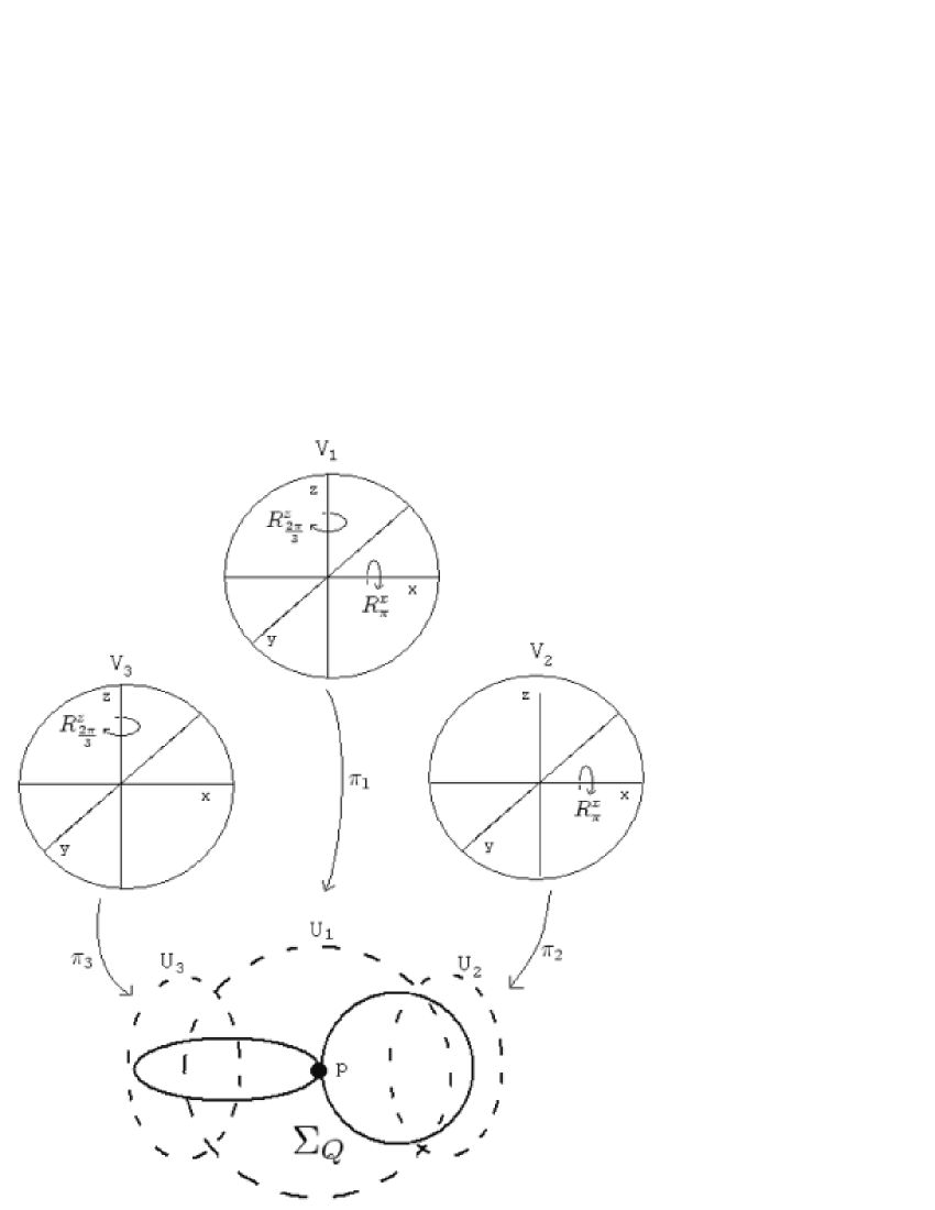
We note, however, that the set is an open 1-manifold diffeomorphic to , and the set is a 0-manifold.
This example serves to illutrate the structure of the set almost in general. For, intuitively, in any chart , vectors tangent to which are invariant under the -action must clearly be tangent to the singular set . Hence, at points where two singular strata ‘run into’ one another, the dimension of the space of tangent vectors decreases. The intersection of the closures of two connected components of , for some , belong to for some .
We state the following obvious corollaries to Proposition 2.2.4 and its proof.
Corollary 2.2.6
With the notation as above, is a set of isolated points. In particular, if is compact, is finite.
Corollary 2.2.7
Let . Then the set of tangent vectors of at is canonically identified with .
2.2.3 Examples of 0-Dimensional Singularities
Our primary interest here is the case of singularities with dimension zero, over which the largest vector space contained in is . For over such points, any vector field must vanish.
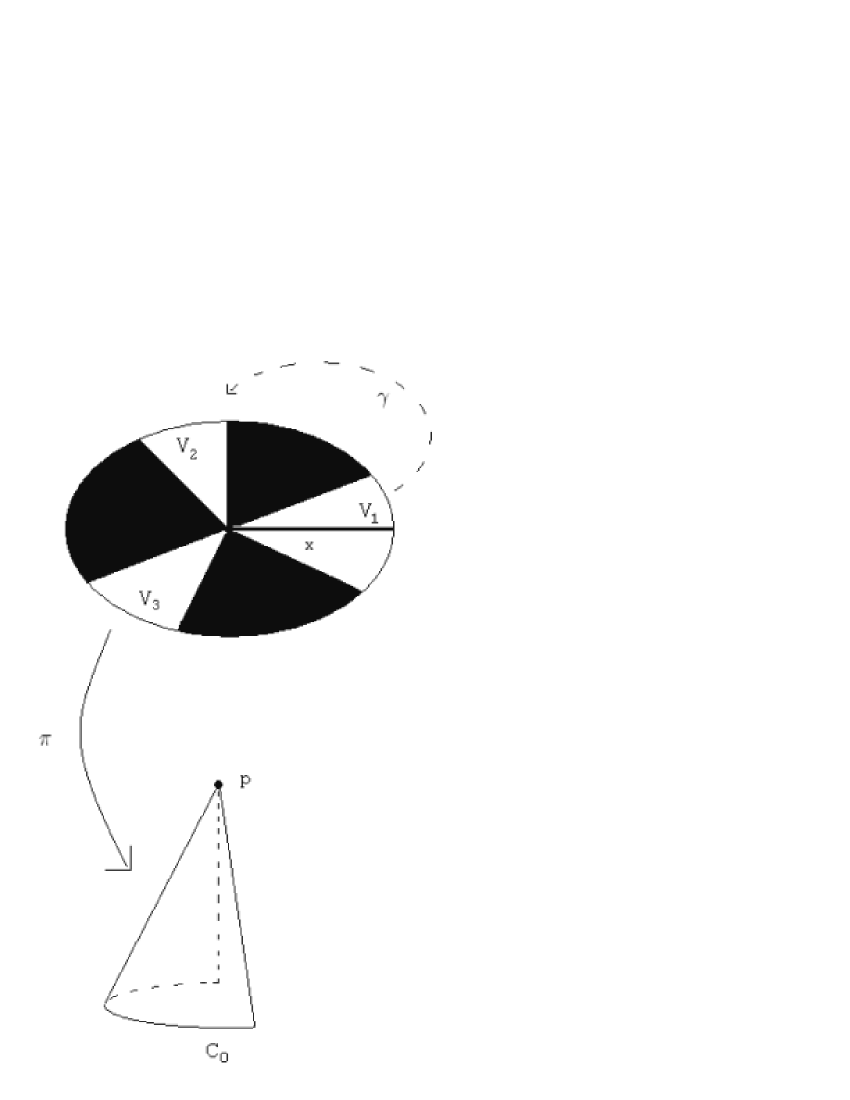
Example 2.2.8
Consider, for example, the cone , which is the quotient of by the group of rotations
where
(see Figure 2.4).
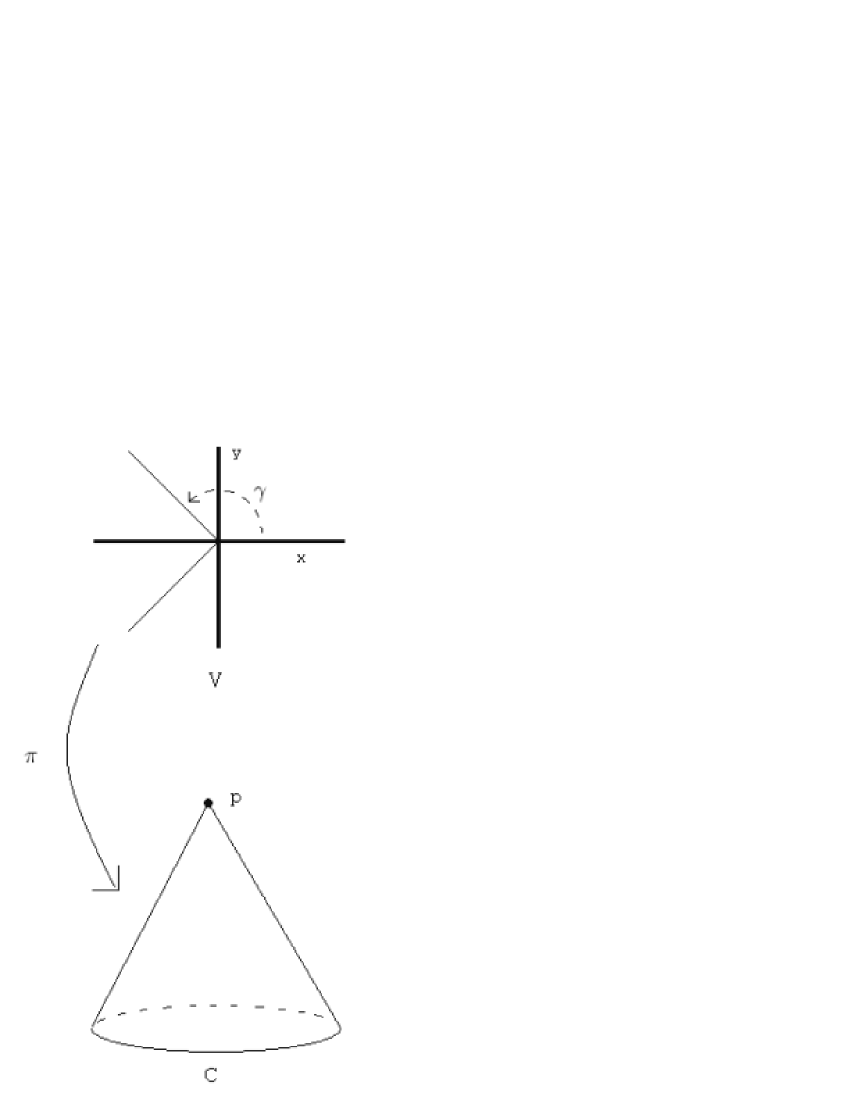
This is clearly an orbifold with one chart where , , and is the quotient map induced by the group action; and one singular point . A vector field on is precisely a -invariant vector field on . However, as has no nontrivial eigenvectors, any vector on the tangent space at is not fixed by , so that any vector field on must vanish at the singular point.
It may be helpful if we develop the tangent space of this previous example explicitly. Any point , , with lift has trivial isotropy group . Hence, the action of on the tangent space is trivial, and the space of tangent vectors is
The set is clearly a smooth 2-dimensional manifold. Moreover, taking a point and an open ball about which does not intersect (small enough so that ), the restriction of to gives a manifold chart of near , and the manifold tangent space of at is exacly the orbifold tangent space of at .
Now, the point has isotropy group . Identifying with in the usual way, we have that as is linear, and (identifying coordinates on with coordinates on via the exponential map; this simply states that the Jacobian of a linear operator is itself). Then is defined to be the set of vectors in which are invariant under the action of the group generated by , which is clearly only the zero vector. Hence, , and the space of tangent vectors to at contains only the zero vector.
The following example is meant to illustrate the limitations of Satake’s definition of an orbifold with boundary (see [20] for the definition). In particular, it is an example in which there is no non-vanishing vector field on the boundary.
Example 2.2.9
Now consider the orbifold with boundary (using Satake’s definition of an orbifold with boundary) defined to be the union of the following subsets of :
(we use standard polar coordinates on ; see Figure 2.5).
Then
is clearly an orbifold with boundary containing one singular point of dimension zero. Hence, as , there is no vector field on which is non-vanishing on the boundary. Indeed, for any such vector field, . Note further that does not admit a product structure near the boundary; i.e. there is no open neighborhood of the boundary in diffeomorphic to .
We should note that these two previous examples are non-compact for simplicity of exposition, but that, by reducing the domain of the charts and patching them together with charts where is the trivial group, the same type of singularity can clearly occur in the case of a compact orbifold: the first as the sole singularity in the -teardrop, and the second in a teardrop which is missing a piece homeomorphic to a disc, where the singularity occurs on the boundary.
For our definition of orbifolds, however, the above cannot occur. Indeed, it is trivial to show (using a chart with linear group action) that if is an orbifold with boundary , then a neighborhood of in is diffeomorphic to . Therefore, for every point on the boundary of , the tangent space contains a one-dimensional subspace independent from . In particular, although may, as an orbifold, contain 0-dimensional singularities, as a subset of , it does not. As well, by Corollary 2.2.6, on a compact orbifold, we need not worry about the existence of a vector field with a finite number of zeros.
Chapter 3 The First Gauss-Bonnet and Poincaré-Hopf Theorems for Orbifolds With Boundary
3.1 Introduction
Our goal in this section is to generalize Satake’s Gauss-Bonnet Theorem for orbifolds with boundary [20] using the more modern definition of an orbifold with boundary. We will see that, with this definition, Satake’s boundary term can be simplified considerably (indeed, in some cases it will vanish).
To this end, a note is necessary. The statemenet of Satake’s Gauss-Bonnet Theorem for orbifolds with boundary refers to an outward-pointing unit normal vector field on the boundary of . In the case that is taken to be an orbifold with boundary as defined by Satake, the boundary may very well contain 0-dimensional singular points (as in the case of the sliced cone in Example 2.2.9), in which case this vector field does not exist—indeed, in such a case there will be no non-vanishing vector field on the boundary. However, our definition does not allow such behavior.
This section follows constructions in [4], [20], and [22]. However, our notation primarily follows that of [22]. Where possible, we state our results and constructions for general orbifold vector bundles, though our primary application will be to the tangent bundle. In particular, many of the definitions will be made in as a general a context as possible to facilitate the proof of the Thom Isomorphism Theorem for Orbifolds (Theorem 3.3.8) in the general case. All orbifolds under consideration are assumed to be reduced.
3.2 The Results on the Level of Differential Forms
3.2.1 The Setup
In this subsection, we fix the context and notation for the rest of the section. Let be a compact, connected, orientable orbifold of dimension with boundary , taking the orientation of to be the orientation inherited from with respect to the outer unit normal vector field. We will use with liberty the fact that that there is a neighborhood of in diffeomorphic to . Let be an orbifold vector bundle over of rank or equipped with a Euclidean metric. Let denote the unit sphere bundle of with respect to the metric, with projection still denoted . Fix a compatible -connection with curvature on . With respect to a local orthonormal frame for , we let denote the component functions on and the basic forms: .
For the specific case where is the tangent bundle of , we require that the metric respect the product structure of near the boundary. In particular, at any point , with respect to any chart and any oriented orthonormal frame field for the fiber at ( as usual), we have that whenever or . Note that in the case of the tangent bundle, .
Let be a vector field on which is non-zero on and has a finite number of fixed points on the interior of . Denote by the geodesic ball about of radius , and for ease of notation, let . Let denote the section of the sphere bundle induced by . We will sometimes require that extend the outer unit normal vector field on , in which case we will use the notation for the vector field and for the induced section of the sphere bundle.
3.2.2 Notes on the Definitions of the Integrands
A note is in order on our definition of the Euler curvature form and its secondary form . These forms, which were originally defined by Chern [4] in the case of the tangent bundle of a closed Riemannian manifold of even dimension, were used by Satake [20] and Sha [22] in generalizations of the Gauss-Bonnet Theorem to the case of closed orbifolds and of the Poincaré-Hopf Theorem to the case of manifolds with boundary, respectively. However, the definitions of the two forms differ slightly, primarily due to Chern’s further developments in [5]. In particular, in [5], Chern extended the definition of these forms to odd-dimensional manifolds and reversed the sign of the Euler curvature form. Hence, some care must be taken with respect to how the various definitions of the forms fit together.
In [4], the forms first appeared on the tangent bundle of a closed Riemannian manifold of dimension . They were called and , respectively, and defined as follows with respect to a frame (again with component functions and basic forms ):
is the Euler curvature form, and
its secondary form on the unit sphere bundle, where
for (as usual, denotes the group of permutations of letters).
In [5], Chern introduced a new definition of the form on both even and odd-dimensional manifolds:
where
for . It is pointed out ([5], page 675) that when is even, the , and hence , reduce to their definitions in [4]. As was mentioned above, the definition of differs from the previous only by a minus sign (so that a sign is introduced in the relationship between the two forms).
The reason for our difficulty is that various authors have since used different conventions regarding the signs of these forms, so that the definitions of the forms are by no means standard. The definitions of Chern in [5] are such that, in the odd dimensional case, the integral of the secondary form on a fiber of the sphere bundle is in the odd-dimensional case, and hence relates to the negative index of the vector field. This, of course, offers no difficulty for closed manifolds, as the index of the vector field is in this case always zero. However, in the case of manifolds with boundary, this leads to a negative sign in the formula, which is undesirable. The reader who may compare our computations to those in [4], [5], [20], [21], or [22] is warned to compare the definitions carefully and take into account the appropriate sign conventions.
We will follow Sha’s notation for the most part, letting denote the Euler curvature form (with respect to the connection ) and its secondary form. Our sign conventions are chosen so that in the resulting formula, the index of the vector field has the same sign in both the even and odd cases. Hence, we will use the following definitions, for an arbitrary vector bundle of rank (again, in the case of the tangent bundle):
is the Euler curvature form, which agrees with the definition of Sha [22]. The secondary form on the unit sphere bundle is
where
We have that on the unit sphere bundle, , where again denotes the bundle projection. Moreover, we have that where is any point in with isotropy . Of course, these relations are preserved up to the sign using the definitions in any of our references (in the case of a manifold, is always equal to ).
3.2.3 The Result of Satake for Orbifolds With Boundary
In [20], we have the following Gauss-Bonnet Theorem.
Theorem 3.2.1
(Satake) Let be an oriented compact Riemannian orbifold with boundary , let be the outward-pointing unit normal vector field on , and let be the induced section of . Then we have
where is oriented by the induced orientation with respect to the outer normal vector field on .
It is noted that the requirement of orientability can be lifted by using the standard reduction to the orientable double-cover.
Here, and are the orbifold Euler characteristic and inner orbifold Euler characteristic of and , respectively, whose definitions we recall (see Appendix A for a discussion of alternate Euler characteristics for orbifolds).
Satake’s definition of the Euler characteristic for a closed orbifold without boundary came from his proof of the Gauss-Bonnet Theorem in this case, with the equation
Since the left-hand side does not depend on the vector field , and the right-hand side does not depend on the metric, this number is an invariant of the orbifold itself. We denote this invariant and refer to it as the orbifold Euler Characteristic. Satake goes on to show how this number can be computed in terms of a suitable triangulation, the existence of such a triangulation since having been demonstrated in [15]. Specifically, if is a triangulation of such that the order of the isotropy group is a constant function on the interior of any simplex , then letting denote this order, we have
Now, in the case that has boundary, the inner orbifold Euler Characteristic is defined similarly, but with respect to a particularly chosen vector field: one which extends the outward unit normal on the boundary of . In this case, given a simplicial decomposition as above, we have
where denotes the collection of simplices which are not completely contained in the boundary.
3.2.4 Computations of in the Case That Extends the Outer Unit Normal Vector Field on
As was pointed out in Sha [22] for the case of manifolds, in the specific case that the vector field extends the outward-pointing normal vector field and is even, if denotes the section of induced by , we have that
on . This is proven as follows:
With a chart and an orthonormal oriented frame field chosen for a point on the boundary such that the are tangent to the boundary of , the form is a sum of terms of the form
for . We have that the is locally equal to in the lift to ; it has coordinates with respect to this frame. Hence, as , we have that vanishes for each . Note that each term either has a factor of for , or has a factor of and a factor of for , in which case . Therefore, each of these terms vanish when composed with , and hence
It will be worthwhile to see how these computations simplify in the case of odd (this is also noted by Sha in [22]). As above, all of the factors vanish except for , but there does exist one which does not contain any such factors:
Moreover, in , we have that the coefficient in every term except those such that (recall that and for ). Hence,
where is understood to be the group of permutations on . So in this case,
Recall that is a frame field for , and that is of dimension . Therefore, the above form is precisely times the Euler curvature form for . In summary,
Hence, in the odd case,
the last equality following from Satake’s Gauss-Bonnet Theorem for closed orbifolds.
3.2.5 The Theorems for Orbifolds With Boundary
With this, we may restate Satake’s result for orbifolds with boundary.
Theorem 3.2.2 (The First Gauss-Bonnet Theorem for Orbifolds with Boundary)
Let be a compact orbifold of dimension with boundary , and let be defined as above in terms of the curvature of a connection . Then
Note that as is defined to be zero in the case that is odd, we have the familiar relation
Example 3.2.3
For example, the solid -football (i.e. the closed ball in with the usual action of via rotations; see [2]) is an orbifold with boundary whose inner orbifold Euler Characteristic is . Its boundary has orbifold Euler Characteristic . This can be easily verified with a simplicial decomposition, or using the fact that the the space is diffeomorphic to and the boundary .
We are now in the position to extend the Poincaré-Hopf Theorem to the case of a compact oriented orbifold with boundary. Begin with the setup given in Section 3.2.1 with and a vector field with a finite number of zeros on the interior of . We require only that does not vanish on the boundary. The index of at is defined in a manner analogous to the integral; if is a chart at and denotes the lift of to , then the index of at is
(see [20]). Of course, for this choice of chart; i.e. is the isotropy group of .
In both the even and odd cases, we have that
on the unit sphere bundle of the tangent bundle. Moreover, at each singular point , we have that
This follows from the fact that the integral of over any fiber of the unit sphere bundle is . The minus sign is due to the fact that the orientation that inherits as a component of the boundary of is the opposite orientation of that used in definition of the index (see for example [8] or [13]). Recall that denotes the union and set .
With this, based on Sha’s proof of the Poincaré-Hopf Theorem for manifolds with boundary, we have the following:
If is even, then
so that
Similarly, if is odd, then as ,
so that
In summary, we state the following.
Proposition 3.2.4
Let be a compact orbifold of dimension with boundary . Let be vector field on which has a finite number of singularities, all of which occuring on the interior of . Then
3.3 The Thom Isomorphism Theorem for Orbifolds
In Section 3.4 below, we will show that, as is the case with manifolds, the cohomology class of the form is an invariant of , and hence does not depend on the various choices made. In order to characterize the cohomology class of in , we need to determine its relationship with the Euler and Thom classes of the tangent bundle . To this end, we develop the Thom Isomorphism Theorem for orbifolds in de Rham cohomology (Theorem 3.3.8).
3.3.1 The Thom Isomorphism in de Rham Cohomology
We begin by stating the following Theorem (taken from [14]). In this case, denotes the set of nonzero vectors in the vector bundle with total space (so that ), and is a typical fiber (with , the set of nonzero vectors in ).
Theorem 3.3.1 (Thom Isomorphism Theorem)
Let be an oriented -plane bundle with total space . Then the cohomology group is zero for , and contains one and only one cohomology class whose restriction
is equal to the preferred generator for every fiber of . Furthermore, the correspondence maps isomorphically onto .
We will be using the Thom isomorphism below in de Rham cohomology, so it will serve us to re-state the theorem in this context. The construction below is based on the work of Schwerdtfeger [21].
Let be a manifold with an -dimensional vector bundle over . Assuming a Euclidean metric on the bundle , let denote the unit disk bundle of (i.e. the set of vectors with ) and the unit sphere bundle. We let denote the projection , as well as its restriction to , , etc. Let , and let be the map .
The cohomology of the pair , then, is studied via forms on relative to (i.e. forms on which vanish on the boundary). We state the following theorem from [21], noting that we have changed his notation and sign convention in a consistent and suggestive manner.
Theorem 3.3.2
(Schwerdtfeger) Let , be forms which satisfy
where denotes the fiber of over an arbitrary point . Let be smooth with
where .
Then the form
is a representative of the Thom class.
Quite clearly, in the case of a manifold, the forms and , as defined above, satisfy these conditions, and hence we may take this to be a definition of the Thom class for (here again, we take the restriction of to the sphere bundle of ). Note that, restricted to ,
so that vanishes on the boundary. Note further that on , .
With this, we have that the map
induces an isomorphism
where we are using the natural isomorphisms and induced in both cases by the inclusion of the latter into the former.
3.3.2 The Case of a Global Quotient
Let be an -dimensional, oriented, closed global quotient orbifold so that is oriented, compact, and smooth and is finite, and let be a -bundle of rank on equipped with a Euclidean metric. Then naturally has the structure of an orbifold vector bundle over . Say that carries a Euclidean metric (which is precisely a -invariant metric on ). Recall that a differential form on is precisely a -invariant differential form on . Hence, if denotes the -invariant -forms on , then the quotient projection
induces
which is clearly an isomorphism of linear spaces. If we extend to , then we have a similiar identification
Throughout this section, let denote the projection of onto (and its various extensions to bundles on and their corresponding orbifold bundles on these ). With and the bundles over and , respectively (with respective projections and ), we let and denote the collection of nonzero vectors in each of these spaces, and the ball bundles, and the sphere bundles, etc.
Let denote the Thom class of the bundle over (tensoring the cohomology group with ), and let be the differential form given by Theorem 3.3.2 which represents the Thom class in de Rham cohomology. In general, if is a -invariant differential form on , we will identify it with the associated differential form on . We denote by its class in and its class in (and respectively, on , , etc.). So in this notation, .
We have that the map
is an isomorphism (again useing the canonical isomorphisms and ).
Note that is -invariant, as it is defined in terms of the forms and , which are -invariant whenever the metric is, and the function can clearly be chosen to be -invariant. Hence, (via its identification with ), and as clearly, represents a cohomology class in .
Consider the map , where . We will represent this map using the isomorphisms and given above, and the obvious isomorphism
Hence, this map can be expressed on forms as for .
Before we deal with , however, we need a lemma which will help us relate and . Essentially, it claims that if a -invariant form is exact in , then it is exact in .
Lemma 3.3.3
Suppose that with . Then there is an with .
Proof:
Using the averaging map, set
Then
Moreover, for each ,
so that is -invariant.
Q.E.D.
Claim 3.3.4
The map defined above is injective.
Proof:
Suppose that represent classes in such that . Hence, .
As and are closed, they represent classes . So as is known to be an isomorphism here, and as , we have that . So there is an such that
Note that, as
and the are -invariant, is -invariant. Applying Lemma 3.3.3, we can take to be -invariant, and hence . So is injective.
Q.E.D.
Claim 3.3.5
The map is surjective.
Proof:
Let be a closed form. Then represents a class , so that as is an isomorphism, there is a closed and an such that . As is closed, is -invariant, so that can be taken to be -invariant. So represents a class in . Moreover, is -invariant, so that can be taken to be, Therefore, is cohomologous to in .
Q.E.D.
Claim 3.3.6
The cohomology class does not depend on the connection.
Proof:
We need only show that the map induced by the quotient projection is injective. for the cohomology class of is unique by Theorem 3.3.1. So suppose for closed and some . Then as is -invariant, can be chosen to be -invariant, so that is in the image of . Hence is exact.
Q.E.D.
Hence, we see that represents a unique cohomology class which induces an isomorphism .
In summary, we state:
Proposition 3.3.7 (The Thom Isomorphism for Global Quotients)
Let be an -dimensional, oriented, closed global quotient orbifold so that is oriented, compact, and smooth and is finite, and let be a -bundle on . Then, with the form as defined above, the map
is an isomorphism. Hence, if denotes the cohomology class in represented by , then the map is an isomorphism. Moreover, does not depend on the metric or connection.
In the next section, we will apply these results locally to a bundle over a general orbifold by considering each set with chart to be a global quotient , and the bundle to be the quotient . However, in these cases, the set is not compact. In order to justify such an application, we note that although Schwerdtfeger’s results only apply to compact manifolds, Theorem 3.3.1 applies in general, so that there is a Thom class in with the desired properties. Moreover, as we can always take to be a bounded open ball in and extend the metric and connection to a larger ball in which contains . Hence, as the Thom class can be characterized by a completely local property (that its restriction to each fiber is the preferred generator of with respect to the orientation), the class of must coincide with the Thom class on the interior of this ball. So in this case, the above construction is still valid.
3.3.3 The Case of a General Orbifold
For the case of a general closed orbifold with orbibundle , we will use the fact that is locally a global quotient; i.e. that each point is contained in a neighborhood which is a global quotient. The proof of the Thom Isomorphism Theorem, then, will involve an induction following Milnor and Stasheff [14]. We note that for each open that is uniformized by , is given the structure of a global quotient orbifold via . Hence, applying the note in the last subsection, the Thom Isomorphism Theorem is known locally.
First, we let carry a Euclidean metric. Then we may take the definition of the Thom class, , as given above, in terms of the global forms and . As , represents a cohomology class , which we define to be the Thom class of (here, and are defined to be the ball bundle and sphere bundle, respectively, of with respect to the metric, as in the last subsection). Note that, for each uniformized , we may give the restricted metric of , and then is the Thom form of . We now proceed with the induction.
Suppose is the union of two open sets, with having chart for , such that each is a bounded ball in , and each acts linearly. Then applying the note above and the case for global quotients, the Thom Isomorphism holds for each . Note further that, as , is also given the structure of a quotient via the uniformization of .
We have the following two Meier-Vietoris sequences (using coefficients in throughout):
and
Using the fact that the isomorphism is known for all but one step in this sequence, we have the following for each ,
Each of the vertical isomorphisms is given by on the level of forms; similarly, by in cohomology (with and appropriately restricted), so that the diagram clearly commutes. Applying the Five Lemma gives us that is also an isomorphism, and that the isomorphism is given by . Hence, we have shown the Thom isomorphism in this case.
Now, suppose is any closed orbifold with orbifold vector bundle of rank , and let be a cover of such that each is uniformized by . If , then is a global quotient, and Thom isomorphism is known. For , assuming as our inductive hypothesis that the Thom isomorphism holds for , applying the above argument to the two sets and shows that it holds for .
With this, we have proven the following.
Theorem 3.3.8 (The Thom Isomorphism for a Closed Orbifold)
Let be a closed oriented orbifold and an oriented orbifold vector bundle of rank over . Let be defined as in Theorem 3.3.2, and then the map
is an isomorphism. Moreover, with respect to each chart , restricts to the preferred generator of (using the isomorphism between and ). In particular, the class of does not depend on the metric or connection.
Note that, by its construction, it is trivial that the restriction of to is (and hence the restriction of to is the cohomology class of in ). Therefore, is closed, and cohomology class it represents in does not depend on the metric. We refer to this class as , the Euler class of as an orbifold bundle. In the case , is simply the Euler class of as an orbifold. In general it does not coincide with the Euler class of the underlying space of , but is a rational multiple thereof.
3.4 The Theorems on the Level of Cohomology
3.4.1 Invariance of the Integrands on the Metric
We return to the case where has boundary, , and . We have the formula (Proposition 3.2.4)
which generalizes the Poincaré-Hopf Theorem to the case of a compact orbifold with boundary. In this section, we characterize the cohomology class of in in order to show that it does not depend on the metric. This section again follows [22].
Recall that on . However, as is isomorphic to where denotes the trivial bundle on of rank 1, and hence that whenever or , clearly vanishes on . So is a closed form on , and hence represents a cohomology class . We have seen that
where is the outward-pointing unit normal vector field on and denotes the cohomology class of in . Moreover, the integral of on a fiber of over a point is . Thus, the following is clear.
Claim 3.4.1
Let where is uniformized by . If is an orientation-preserving isometry from to a fiber of the sphere bundle of (i.e. the sphere bundle pulled back over ), then then , where denotes the canonical generator of .
Note that in the case where , we can identify with via , so that .
With this, we may characterize the class by developing the Gysin sequence of the tangent bundle. Let now denote the restriction and the nonzero vectors of . We follow Milnor and Stasheff [14] and Sha [22]. All coefficient groups are understood to be .
To simplify the notation, we let denote . We have the cohomology exact sequence
We may replace with using the natural isomorphism induced by . Similarly, applying the Thom Isomorphism, we may replace with . The restriction map composed with results in (where is the Euler class of the orbifold bundle ):
Now is canonically isomorphic to , so that again using for the restricted projection we obtain
However, we have noted that the Euler class of is zero, so that setting , we obtain
Finally, we choose to be an isometry (as above) to a fiber over a point with trivial isotropy, so that
gives the split exact sequence
With this, as is a left inverse of (recall that is the section induced by the outward unit normal vector field on ), we have . With respect to this decomposition, based on the properties of , factors into . Hence, this characterizes , and in particular shows that it does not depend on the choices made in the definition of . Note that choosing to map to the fiber over a singular point will introduce a coefficient of in the above expression.
With this, Proposition 3.2.4 becomes
Theorem 3.4.2 (The First Poincaré-Hopf Theorem for Orbifolds with Boundary)
Let be a compact orbifold with boundary . Let be vector field on which has a finite number of singularities, all of which occuring on the interior of . Then
Chapter 4 The Gauss-Bonnet Integrand in Chen-Ruan Cohomology
4.1 Introduction
The goal of this chapter is to examine the results of the previous chapter in terms of the orbifold cohomology developed in [3]. In particular, we are interested in cohomology classes corresponding to those of and . Roughly speaking, the Chen-Ruan orbifold cohomology of an orbifold contains the usual cohomology of as a direct summand, but contains as well the cohomology groups of the twisted sectors, corresponding to irreducible components of the singular set of . With respect to this decomposition, the new characteristic classes will project to the usual ones. They will, however, have additional lower-degree terms, which correspond to the contributions of the singular sets. Our results, then, will involve the Euler characteristic of the underlying topological space instead of the orbifold Euler characteristic. Taking the point of view that an orbifold structure is a generalization of a differentiable structure on a manifold, we obtain results for orbifolds much more in keeping with the original Gauss-Bonnet and Poincaré-Hopf Theorems.
Throughout this chapter, orbifolds and orbifolds with boundary will be taken to admit almost complex structures.
4.2 Chen-Ruan Orbifold Cohomology
In this chapter, we will be working with the orbifold cohomology theory developed by [3]. We will not develop this cohomology theory here, but will collect a summary for the sake of making the notation explicit. For the most part, we follow the notation in [3], [17], and [18].
Let be an orbifold, and select for each a chart at . Then the set
(where is the conjugacy class of in ) is naturally an orbifold, with local charts
where is the fixed point set of in and is the centralizer of in . If is closed, then is closed, but it need not be connected, and its connected components need not be of the same dimension. An equivalence relation can be placed on the elements of the groups so that if denotes the set of equivalence classes and the equivalence class of ,
where
The map with , is a map.
If is an almost complex orbifold, a function is defined which is constant on the connected components of . If denotes the codimension of in , then , with equality only when . This is called the degree shifting number of . The orbifold cohomology groups are defined by
where the groups on the right side are the usual de Rham cohomology groups of the orbifolds .
Since each can be realized as a subset of , geometric constructions (i.e. bundles and their sections) on can be naturally extended to geometric constructions on . In what follows, we wish to extend the characteristic classes of bundles over to characteristic classes of associated bundles over ; however, pulling back such bundles via will be insufficient. In particular, if is a rank orbibundle and is a singular point contained in a singular set of dimension , then the maximal vector space in a fiber over has dimension . This implies that any -form on is zero on (recall that it is required of sections of orbibundles that for each , is contained in the subspace of the fiber over which is fixed by ). In particular, any form representing the Euler class of is zero at , so that the pull-back of this form will be zero on each connected component of of dimension is less than . This is particularly disappointing in the case of the tangent bundle, in that no twisted sectors make contributions to the Euler class.
Instead, we will associate to each bundle a bundle whose dimension on each component is equal to , where is the rank of , is the dimension of , and is the dimension of (i.e. the rank of minus the codimension of in ). We will then apply the Chern-Weil construction to a connection on in order to define characteristic classes in which are invariants of .
4.3 Chen-Ruan Orbifold Cohomology for Orbifolds with Boundary
In this section, we generalize orbifold cohomology to the case of orbifolds with boundary. This is a straightforward generalization following [3].
Let be an -dimensional orbifold with boundary . Again, we let
Then we have:
Lemma 4.3.1
The set is naturally an orbifold with boundary, with projections given by
for each chart at . Here, denotes the fixed point set of in and is the centralizer of in . If is compact, then so is . The map is a map.
For the proof of this lemma for the case that does not have boundary, see [3]. The proof for the case with boundaries is identical.
Lemma 4.3.2
Let be an orbifold with boundary . Then .
Proof:
Let be a point in . Then is contained in a chart of the form , induced by a chart for at . As is in th boundary of , is diffeomorphic to for some . However, as , its fixed-point set in is a subspace, so that must be diffeomorphic to (where is the dimension of ). Therefore, .
Conversely, suppose is a point in the boundary of , and let be a chart at . Then , and any lift of into is contained in . For any , the element of is covered by the chart , and any lift of into is clearly an element of . Therefore, represents a point in . With this, we note that any point arises in such a way, and is contained in a chart for induced by a chart for (and hence by a chart for ).
Q.E.D.
We review the description of the connected components of , treating the case that has boundary.
Let be an orbifold chart for at a point , and let . Let be an orbifold chart at with , and then the definition of an orbifold gives us an injection . The injective homomorphism is well-defined up to conjugation, so that it defines for each conjugacy class a conjugacy class . We say that , which defines an equivalence relation on the elements of the local groups. Let denote the equivalence class of a group element ; note that it is no longer important to state the particular local group from which was taken. For each equivalence class, we let
and then . In particular, following [3], we call the nontwisted sector and each for a twisted sector. It is worth noting that in the case that with a manifold and a finite group, the equivalence relation reduces to that of conjugation in .
Example 4.3.3
For the case of a point with the trivial action of a finite group (see Example 2.1.8), the above defined equivalence relation reduces to conjugation within the group, and consists of one point for each conjugacy class. For an element , the point corresponding to has the trivial action of , the centralizer of .
Example 4.3.4
If is the -teardrop (see Example 2.1.9), then has connected components. The nontwisted sector is diffeomorphic to , while each of the other components are points with the trivial action of .
Example 4.3.5
For where acts via the antipodal map (see Example 2.1.10), has two connected components, one diffeomorphic to and one given by a point with trivial -action.
Example 4.3.6
Consider the case where is the --solid hollow football (see Example 2.1.11) with and relatively prime. Then has connected components. The component corresponding to the identity element (in both groups) is diffeomorphic to . Each of the other components is diffeomorphic to a closed interval with the trivial action of or (there are components with trivial -action and components with trivial -action).
If , then the equivalence relation on conjugacy classes defines an isomorphism between the two , and is a global quotient. Then there are exactly connected components of : one, corresponding to the identity in , is diffeomorphic to , while each of the others is given by with trivial -action (these two pieces correspond to the fixed-point set of the nonidentity elements of , which lie on the -axis).
If and are not relatively prime, then letting , can be expressed as a global quotient of the --football by , and then the structure of can be determined using both of the above constructions.
Example 4.3.7
Suppose is an orbifold with boundary homeomorphic to the closed 3-disk whose singular set, located on the interior of the disk, is that given in Example 2.2.5. Then there are six equivalence classes in , each containing exactly one element of . The nontwisted sector is again diffeomorphic to . The twisted sector corresponding to the equivalence class of is given by with a trivial -action. The twisted sectors corresponding to and are both given by with trivial -action. The twisted sectors corresponding to the elements and are both points with trivial -action.
Now, suppose admits an almost complex structure . As in the case without boundary, inherits an almost complex structure from (note that this almost structure is on , which is not generally the same as . For each and chart at , the almost complex structure defines a homomorphism where is the dimension of over . For each , can be expressed as
with the order of and . Following [3], define
and then defines a map which is constant on each . Let for any . We refer to as the degree shift number of .
Definition 4.3.8
Let be an orbifold with boundary that admits an almost complex structure . The relative orbifold cohomology groups are defined to be
where is either the singular or de Rham relative cohomology group of .
In the sequel, we will examine analogs of the theorems of the previous chapter with the characteristic classes taken to be elements of these cohomology groups.
4.4 The Gauss-Bonnet and Poincaré-Hopf Theorems in Chen-Ruan Cohomology
We begin with a lemma.
Let be a closed orbifold of dimension , and let be an orbifold vector bundle of rank . Suppose further that has the following property: for any chart at , and any subgroup of , the codimension of the fixed point set of in the fiber is equal to the codimension of the fixed point set of in (or is zero if the codimension of the fixed point set in is greater than the rank of ). This is the case, for instance, for the tangent and cotangent bundles, their exterior powers, etc. (which can be verified using a metric and the exponential map). As is an orbifold, we may apply the construction to form .
Lemma 4.4.1
With , as above, is naturally an orbifold vector bundle over , and the rank of on each connected component of dimension is . In particular, the fiber of is zero on any with codimension larger than .
Note that the restriction on the group actions on is stronger than the requirement that be a so-called good orbifold vector bundle (see [17] for the definition; our definition of orbifold vector bundle coincides with Ruan’s definition of a good orbifold vector bundle). However, we will be applying this result to the tangent bundle only. For general (good) orbifold vector bundles, is still naturally a vector bundle over , but the rank of over a connected component of depends on the group action on .
Proof:
First, we note that as the local groups and injections of are precisely those of , the set is identical for both orbifolds. Let be defined by . Then is certainly well-defined, as is fixed by a group element if is.
Fix a point , where and , and let denote the projection of . Then by the definition of , is contained in a uniformizing set induced by a uniformizing set of . Moreover, we can take this orbifold chart for to be a uniformizing system of the rank orbifold bundle induced by a system near in . Hence, , , and .
By our definition of orbifold vector bundle, the kernel of the action on the fiber over a point is the kernel of the action on . Hence, the fixed point set of in is (or the zero vector space if ), where is the dimension of (i.e. minus the codimension of in ). If we define the map by projection onto the first factor, then for any (say ), we have that
and hence that .
Hence,
is a rank uniformizing system for a bundle over the uniformizing system about .
We have that any point of is contained in a bundle uniformizing system over a uniformizing system of with projection . Given a compatible cover of (which can be taken to be induced by a compatible cover of ) an injection is always the restriction of an injection (by [20], Lemma 1, there is a bijection between elements of and such injections; hence, restricting to the subgroup decreases the number of injections). Then the transition map is simply the restriction of the corresponding transition map for to the fixed-point set . Therefore, these uniformizing systems patch together to give the structure of an orbibundle over .
Q.E.D.
Applying the above argument to the tangent bundle shows that ; i.e. the tangent bundle of is the collection of twisted sectors of the tangent bundle of . Similarly, the constructions of the cotangent, exterior power, and tensor bundles commute with this construction. Moreover, any smooth section of the bundle naturally induces a smooth section of the bundle via .
Theorem 4.4.2 (The Second Gauss-Bonnet Theorem for Closed Orbifolds)
Let be a closed oriented orbifold of dimension , and suppose carries a connection with curvature . Let denote the induced connection on , and let denote its curvature. Let denote the Euler curvature form of , defined on , and then
the Euler characteristic of the underlying topological space of . Moreover, if is almost complex, then represents an element of the cohomology ring which is independent of the connection on .
Proof:
We first note that on each , is a representative of the Euler class of , so that, by the Gauss-Bonnet theorem for orbifolds,
where again the sum is over the set of equivalence classes of local group elements. Note that is closed, so that it has a finite number of connected components (i.e. is finite).
Now, let be a simplicial decomposition of such that for each simplex , the order of the isotropy group of is constant on the interior of (see [15]). Let be the simplicial decomposition of induced by , and for each , denote by the corresponding simplex in which lies in . As is finite, let be an enumeration of the simplices in so that .
For each , let be a point on the interior of the simplex, and let be an element of such that . Note that the order of the conjugacy class of in , as well as the orders and , are independent of the choices of and . Hence,
To finish the proof, suppose is almost complex, and note that for each , as is on its own an orbifold, is a representative of the Euler class of in . Denote this class , and then represents the element
which is an invariant of the connection. Note that if has dimension , then is an element of .
Q.E.D.
Note that it is inessential that be defined as being induced by a connection on ; the theorem holds if we begin with an arbitrary connection on .
In the case of an almost complex, reduced orbifold of dimension , the cohomology group is isomorphic to the de Rham group . Hence, the top part of is a representative of the Euler class of with respect to this isomorphism. In the case that is not reduced, if denotes the number of elements of whose representatives act trivially, then is isomorphic to ( copies). Then the top part of is copies of the Euler curvature form.
Definition 4.4.3
Let be an almost complex, closed, oriented orbifold, a vector bundle, and the induced bundle. The orbifold Euler class is the cohomology class represented by in for some connection on with curvature .
Corollary 4.4.4 (The Second Poincaré-Hopf Theorem for Closed Orbifolds)
Let be a vector field on the closed orbifold with a finite number of zeros, and let be the induced vector field on . Then
Proof:
This follows from the Poincaré-Hopf theorem for closed orbifolds [20], applied to each connected component of . Note that, as vector fields must be tangent to the singular set, a vector field with a finite number of zeros on will induce a vector field with a finite number of zeros on .
Q.E.D.
Again, it is inessential that we begin with a vector field on and pull back to .
4.4.1 Examples
Example 4.4.5
We start with the example of a single point with the trivial action of a finite group . In this case, the equivalence relation reduces to conjugation in the group. Then , and the degree shifting number for each (see [3]).
The contribution of each connected component of to the orbifold cohomology is in , so that if is the number of conjugacy classes in ,
The curvature form of each point is the function , so that summing this value over each of the connected components of gives
Example 4.4.6
Let denote the -teardrop, and then . The group acts trivially on each , so that the orbifold Euler characteristic of each of these points is . Then , so that
4.5 The Case With Boundary
We return to the case of an orbifold with boundary. A modification of the proof of 4.4.2 shows:
Theorem 4.5.1 (The Second Gauss-Bonnet Theorem for Orbifolds with Boundary)
Let be a closed orbifold of dimension with boundary , and suppose carries a connection with curvature . Let, , , etc. be defined as in the previous section, and then
If is almost complex, then represents an element of the cohomology ring which is independent of the connection on .
Note that .
Proof:
Again, by the Gauss-Bonnet theorem for orbifolds with boundary,
Using a simplicial decomposition of as above and the same counting argument, we have
Q.E.D.
Clearly, in the case where the dimension of is even, this formula becomes
and in the case where is odd,
We now return to the proof of Proposition 3.2.4. Let be defined in the natural way by taking the sum of on each connected component of . Then the relation is immediate, as it is true on each connected component. Again, let denote the extension of the vector field to . We modify the proof of Proposition 3.2.4 by applying in the first step Theorem 4.5.1 instead of the Theorem 3.2.2 as follows.
If the dimension of is even, then
and hence
Note that the singular points are taken to be those of , and hence the contains balls each singular point of .
Making the identical modification to the proof in the case that is odd, we obtain
and hence
Now, note that in the case that admits a complex structure, as the cohomology class of is independent of the connection chosen, the cohomology class of in is similarly independent. In fact, it is clear that we can define to be the sum of the cohomology classes of the forms defined on each connected component of from the connection, and then would be a representative of the cohomology class . Hence, we have proven
Theorem 4.5.2 (The Second Poincaré-Hopf Theorem for Orbifolds with Boundary)
Let be a compact oriented orbifold with boundary , and suppose admits an almost complex structure. Let be vector field on which has a finite number of singularities, all of which occuring on the interior of . Then with , , etc. defined as above, we have
Here, refers to the integral of any form representing the cohomology class over the orbifold ; we have chosen to use this notation to emphasize the fact that the value of this integral is independent of the particular representative of chosen.
References
- [1] A. Adem and Y. Ruan. Twisted orbifold -theory. math.AT/0107168, 2001.
- [2] J. Borzellino. Riemannian Geometry of Orbifolds. PhD thesis, UCLA, 1992.
- [3] W. Chen and Y. Ruan. A new cohomology theory for orbifold. math.AG/0004129, 2001.
- [4] S.S. Chern. A simple intrinsic proof of the Gauss-Bonnet formula for closed Riemannian manifolds. Ann. of Math., 45:747–752, 1944.
- [5] S.S. Chern. On the curvatura integra in a Riemannian manifold. Ann. of Math., 99:48–69, 1974.
- [6] L. Dixon, J. Harvey, C. Vafa, and E. Witten. Strings on orbifolds. Nucl. Phys. B, 261:678–686, 1985.
- [7] C. Farsi. -theoretical index theorems for good orbifolds. Proceedings of the AMS, 3:769–773, 1992.
- [8] V. Guillemin and A. Pollack. Differential Topology. Prentice-Hall, Inc., Englewood Cliffs, New Jersey, 1965.
- [9] T. Kawasaki. The signature theorem for -manifolds. Topology, 17:75–83, 1977.
- [10] T. Kawasaki. The index of elliptic operators over -manifolds. Nagoya Math. J., 84:135–157, 1981.
- [11] C. Liang. Vector fields on -manifolds, and locally free -actions on manifolds. Indiana University Mathematics Journal, 27:349–352, 1978.
- [12] G. Segal M.F. Atiyah. On equivariant Euler characteristics. J. Geom. Phys., 4:671–677, 1989.
- [13] J. Milnor. Topology from the Differentiable Viewpoint. The University Press of Virginia, Charlottesville, 1965.
- [14] J. Milnor and J. Stasheff. Annals of Mathematical Studies 76: Characteristic Classes. Princeton University Press and University of Tokyo Press, Princeton, New Jersey, 1974.
- [15] I. Moerdijk and D. A. Pronk. Simplicial cohomology of orbifolds. math.alg/9708021, 1997.
- [16] S. S. Roan. Minimal resolutions of Gorenstein orbifolds in dimension three. Topology, 35:489–509, 1996.
- [17] Y. Ruan. Orbifold Gromov-Witten theory. math.AG/0103156, 2001.
- [18] Y. Ruan. Stringy geometry and topology of orbifolds. math.AG/0011149, 2001.
- [19] I. Satake. On a generalization of the notion of manifold. Proc. Nat. Acad. Sci. USA, 42:359–363, 1956.
- [20] I. Satake. The Gauss-Bonnet theorem for -manifolds. Journ. Math. Soc. Japan, 9:464–492, 1957.
- [21] B. E. Schwerdtfeger. On Explicit Furmulas for the Differential Forms in the Thom Class. PhD thesis, University of Bonn, 1979.
- [22] J. P. Sha. A secondary Chern-Euler class. Ann. of Math., 159:1151–1158, 1999.
- [23] E. A. Stanhope. Hearing Orbifold Topology. PhD thesis, Dartmouth College, 2002.
- [24] W. Thurston. The Geometry and Topology of 3-Manifolds. Lecture Notes, Princeton University Math Dept., Princeton, New Jersey, 1978.
Appendix A A Note on Orbifold Euler Characteristics
This note is intended to clarify the various definitions of Euler Characteristics for that have been given for orbifolds and preclude any confusion which may arise. Throughout, let be a compact oriented orbifold and let denote its underlying topological space.
The first orbifold Euler characteristic was defined by Satake in [20], and was originally denoted . This is the orbifold Euler characteristic used in this paper, and which we have denoted . It was defined as the index, in the orbifold sense, of a vector field on with isoloated singularities, or equivalently as the integral, in the orbifold sense, of the Euler curvature form , defined in terms of an orbifold connection on . In general, it is a rational number. If denotes the cohomology class of and the usual Euler class of the underlying space of , then using the isomorphism between the de Rahm cohomology of as an orbifold and the singular cohomology of , it is easy to see that
In many ways, this Euler characteristic plays the role of the usual Euler characteristic of a manifold; as was discussed in Chapter 3, it can be defined in terms of suitable triangulation of the orbifold.
In the case that is the quotient of a manifold by a finite group, another orbifold Euler number was defined in [6] as
where denotes the fixed-point set of (see also [12], where this is shown to be the Euler characteristic of the equivariant -theory ). In [16], this definition is generalized to the case of a general complex orbifold with groups acting as subgroups of as follows: If denotes for each the number of conjugacy classes in the isotropy subgroup , then define
Note that the sum on the right has finitely many non-zero terms. Roan shows that this definition coincides with that of Dixon et. al. [6] in the case of a global quotient, and moreover that it does not coincide with the usual Euler characteristic of the underlying space of unless is nonsingular.
Similarly, in [1], the formula for is genearlized to general orbifolds by defining
Here, denotes the orbifold -theory of , which is defined using complex orbifold vector bundles over and generalizes the equivariant -theory of .
We note that in the case of a reduced orbifold, these two invariants and coincide. Indeed, using the notation of Chapter 4, for each , coincides with the number of distinct such that . Hence, for each positive integer , the preimage of in via the projection is a -fold disjoint covering. Therefore, we have that
The last equality follows from the decomposition theorem for orbifold -theory of Adem-Ruan ([1] Theorem 5.1, Corollary 5.6).
Appendix B Relation to the Index Theorem for Orbifolds
Let be a compact orbifold that admits an almost complex structure, its (orbifold) tangent bundle. Let and be two orbifold vector bundles over , and an elliptic pseudodifferential operator from the smooth sections of to those of . Then if denotes the projection of the tangent bundle, the symbol of gives an isomorphism off of the zero-section of , and hence an element of .
Let denote such a class in the orbifold -theory of . Let , etc. be defined as in Chapter 4, and let denote the induced bundles on . Let denote the induced bundle restricted to the connected component of , and let denote the class of in with the symbol given by the restriction of . With this setup, Kawasaki [10] showed that the orbifold index
is given by
(see also [7]). Here, ch denotes the Chern character of (chch), and the Todd class of te (complexified) tangent bundle.
We we may define the orbifold Chern character of a complex vector bundle and the orbifold Todd class in an analogous manner to the orbifold Euler class: to a bundle with connection we associate the induced bundle over with connection , and then construct the the Chern character and Todd class from the curvature of this connection in the usual manner (the bundle is taken to be the tangent bundle in the case of the Todd class). It is clear that these forms represent elements of that are independent of the connection, and that they can be given as a sum of ordinary characteristic classes of the . In other words, we have
and
We note that the factors appear in the above formula because Kawasaki worked with a definition of orbifold which required that it was reduced. Hence, his correspond to our , and the corresponding factors are built into our definition of the integral.
With this, by reversing the orientation of the odd-dimensional components of , Kawasaki’s index formula can be written as
We note that the cup product here is not the orbifold cup product defined in [3], but rather the pointwise product induced by the wedge product. In particular, forms on cupped with forms on yield when .