Die vorliegende Arbeit wurde von der Mathematisch - naturwissenschaftlichen Fakultät der Universität Zürich auf Antrag von Prof. Dr. Thomas Kappeler und Prof. Dr. Viktor Schroeder als Dissertation angenommen.

Abstract

Consider a closed, smooth manifold $M$ of nonpositive sectional curvature. Write $p:UM\rightarrow M$ for the unit tangent bundle over $M$ and let ${\cal R}_{>}\subset UM$ denote the subset consisting of all vectors of higher rank. This subset is closed and invariant under the geodesic flow $\phi$ on $UM$. We will define the structured dimension $\operatorname{s-dim}R_{>}$ which, essentially, is the dimension of the set $p({\cal R}_{>})$ of base points of ${\cal R}_{>}$.

The main result holds for manifolds with $\operatorname{s-dim}{\cal R}_{>}<{\dim M}/2$: For every $\epsilon>0$ there is an $\epsilon$-dense, flow invariant, closed subset $Z_{\epsilon}\subset UM\backslash{\cal R}_{>}$ such that $p(Z_{\epsilon})=M$. For every point in $M$ this means that through this point there is a complete geodesic for which the velocity vector field avoids a neighbourhood of ${\cal R}_{>}$.

Zusammenfassung

Gegeben sei eine geschlossene, glatte Mannigfaltigkeit $M$ nichtpositiver Schnittkrümmung. Das Einheitstangentialbündel sei mit $p:UM\rightarrow M$ bezeichnet und die Teilmenge aller Vektoren höheren Ranges mit ${\cal R}_{>}\subset UM$. Diese Teilmenge ist abgeschlossen und invariant unter dem geodätischen Fluss $\phi$ auf $UM$. Wir definieren die Strukturdimension $\operatorname{s-dim}{\cal R}_{>}$ von ${\cal R}_{>}$, die, im Wesentlichen, die Dimension der Fußpunktmenge $p({\cal R}_{>})$ misst.

Das Hauptergebnis gilt unter der Bedingung, dass $\operatorname{s-dim}{\cal R}_{>}<(\dim M)/2$ gilt: Für jedes $\epsilon>0$ gibt es eine $\epsilon$-dichte, flussinvariante, abgeschlossene Teilmenge $Z_{\epsilon}\subset UM\backslash{\cal R}_{>}$, für die gilt $p(Z_{\epsilon})=M$. Dies bedeutet, dass es durch jeden Punkt in $M$ eine vollständige Geodäte gibt, deren Geschwindigkeitsfeld eine Umgebung von ${\cal R}_{>}$ vermeidet.

Danksagung

Notwendige und hinreichende Bedingung für das Entstehen dieser Arbeit war die exzellente Betreuung durch meinen Doktorvater Prof. Viktor Schroeder. Ich möchte ihm danken für viele interessante Gespräche im Laufe der letzten Jahre und dafür, dass er sich stets Zeit für mich nahm, wenn ich eine Frage hatte und er nicht gerade für ein halbes Jahr in Chicago weilte.

Meinen Zimmerkollegen Thomas Foertsch und Michael Scherrer, sowie allen anderen Institutsmitgliedern danke ich für das angenehme Arbeitsklima am Institut für Mathematik.

Durch diverse Veranstaltungen haben Prof. Ruth Kellerhals und Prof. Bruno Colbois es in den letzten Jahren verstanden, für einen regelmässigen Kontakt zwischen den mathematischen Instituten vieler schweizerischer Universitäten zu sorgen. Insbesondere die Möglichkeit, andere Doktoranden aus meinem Gebiet kennenzulernen und mit ihnen gemeinsam neue Dinge zu erarbeiten, hat mir oft neue Motivation für meine Arbeit gegeben.

Meinen Eltern danke ich für das Vertrauen in meine Fähigkeiten, welches sie nie verloren haben, und für ihre fortwährende Hoffnung, dass meine Handschrift eines Tages leserlich sein wird.

Zuletzt möchte ich meiner Freundin Anke danken, dafür, dass sie diese Arbeit fehlergelesen hat, für ihre Unterstützung und für ihre schier unerschöpfliche Geduld insbesondere in den letzten Wochen vor dem Abgabetermin.

Danke schön

Bert Reinold

Zürich, im Juli 2003

Contents

1. Zusammenfassung
2. Danksagung
3. 1 Preliminaries
   1. 1.1 Introduction
   2. 1.2 Structure of this Thesis
   3. 1.3 Notation
   4. 1.4 Manifolds of Nonpositive Sectional Curvature
4. 2 Rank and Flatness
   1. 2.1 Horizontal and Vertical Structure
   2. 2.2 Flats and Jacobi Fields
5. 3 Sets of Constant Rank
   1. 3.1 Subanalytic Sets
   2. 3.2 Compact Real Analytic Manifolds
   3. 3.3 s-Dimension
6. 4 Spheres and Horospheres
   1. 4.1 Spheres and Limits of Sphere Segments
   2. 4.2 Flats on a Horosphere
7. 5 Hyperbolicity of Rank One Vectors
8. 6 Avoiding a Rank One Vector
   1. 6.1 Idea
   2. 6.2 Choice of Constants
   3. 6.3 Construction
   4. 6.4 The Construction Has the Desired Properties
9. 7 Avoiding Subsets of Small s-Dimension
   1. 7.1 Avoiding the Unit Tangent Bundle of a Submanifold
   2. 7.2 Respecting the $r$-Sphere Foliation of $UX$
10. 8 Avoiding Higher Rank Vectors
    1. 8.1 Rough Idea for a Single Vector
    2. 8.2 Construction of the Maps $v_{i}$
    3. 8.3 Choice of Constants
    4. 8.4 Construction of a Ray
    5. 8.5 The Construction Has the Desired Properties
11. 9 From Rays to Geodesics
12. A Basics

1 Preliminaries

Before going into detail the introduction in Subsection 1.1 will give a rough outline of what this thesis is concerned with. In Subsection 1.2 the structure of the text is explained section by section. Then Subsection 1.3 will introduce the main notation used throughout the thesis. The theory of Riemannian manifolds of nonpositive curvature as far as considered well known is summed up in Subsection 1.4 for reference.

1.1 Introduction

Given a complete Riemannian Manifold $M$ there is a natural action of $\mathbb{R}$ on the unit tangent bundle $UM$, which is called the geodesic flow and is denoted by

$$\phi:\mathbb{R}\times UM\rightarrow UM.$$

If $\gamma_{v}$ denotes the unique geodesic defined by the initial condition $\dot{\gamma}_{v}(0)=v$ then $\phi_{t}(v)$ is the tangent vector to $\gamma_{v}$ at time $t$

$$\phi_{t}(v)=\frac{d}{ds}\big{|}_{s=t}\gamma_{v}(s).$$

Flow Invariant Subsets of $UM$

Suppose $\gamma_{v}$ is a simply closed geodesic of length $l$. Then the orbit of $v$ under the geodesic flow is isometric to a circle of perimeter $l$. This is the simplest example of a flow invariant subset of $UM$.
Another simple example of a flow invariant subset of $UM$ is the unit tangent bundle $UN$ of a totally geodesic submanifold $N\subset M$.
What other examples of flow invariant subsets of $UM$ can we think of?
In the case where $M$ is a compact manifold of strictly negative sectional curvature, there are many interesting results. E. g. the geodesic flow is ergodic and for almost every geodesic $\gamma$ in $M$ the set $\dot{\gamma}(\mathbb{R})$ is dense in $UM$. There are many references for these results, see for example [Pesin1981].

From Negative to Nonpositive Curvature

Neither ergodicity nor the existence of a geodesic dense in $UM$ holds for the flat torus. But what about those manifolds that are neither flat nor strictly negatively curved?
The manifolds of nonpositive curvature are classified by their rank. The rank of a geodesic is defined to be the maximal number of linearly independent parallel Jacobi fields along that geodesic. For a manifold the rank is the smallest rank of its geodesics.
By a result of Werner Ballmann [BGS, Appendix 1] closed manifolds of higher rank (i. e. rank greater than one) are either products or locally symmetric spaces.
However, manifolds of rank one are similar to manifolds of negative curvature in many aspects. We will use the fact that geodesics in the vicinity of rank one vectors show a behaviour similar to the behaviour of geodesics in hyperbolic space rather than in Euclidean space (compare Proposition 5.2).

Objective

The aim of this thesis is to generalize an unpublished result of Keith Burns and Mark Pollicott for manifolds of constant negative curvature to the rank one case.
For a compact manifold $M$ of constant negative curvature and a given vector $v_{0}\in UM$, there is a subset $Z\subset UM$ with the following properties:

$$\underset{\,\qquad t\in\mathbb{R}\qquad\,}{\forall}\quad\phi_{t}(Z) =Z$$ (flow invariant)

$$\underset{v_{0}\in{\cal W}\subset UM\text{ open}}{\exists}\quad{\cal W}\cap Z =\emptyset$$ (not dense)

$$p(Z) =M.$$ (full)

The construction works in a complete (not necessarily compact) Riemannian manifold $M$ of dimension at least three and curvature bounded away from zero as Viktor Schroeder showed in [Schroeder2001].
For a compact manifold $M$ of nonpositive curvature Sergei Buyalo and Viktor Schroeder proved in  [whoknows] that this set $Z$ can be constructed for every vector $v_{0}\in UM$ of rank one. To construct $Z$ they proved the following proposition:

Proposition 1.1 ([whoknows])

Let $M$ be a manifold of nonpositive curvature and dimension at least three and let $v_{0}\in UM$ be a vector of rank one. Then for any point $o\in M$ we can find an $\epsilon>0$ and a geodesic $\gamma_{o}$ passing through $o$ with the property that the distance between $\dot{\gamma}_{o}(t)$ and $v_{0}$ is greater than $\epsilon$ for all $t\in\mathbb{R}$.

If we take a closer look at the proof we notice that $\epsilon$ can be chosen to depend continuously on $o$ and thus if $M$ is compact we can choose $\epsilon$ globally for all $o\in M$. Thus if we define

$$Z:=\underset{o\in M}{\bigcup}\dot{\gamma}_{o}(\mathbb{R})$$

and ${\cal W}$ denotes the $\epsilon$-neighbourhood of $v_{0}$ in $UM$, we have the desired properties.

So for every rank one vector $v_{0}$ there is a flow invariant, full subset of $UM$ the complement of which contains a neighbourhood of $v_{0}$.
In fact, $Z$ can be chosen to be $\epsilon^{\prime}$-dense for some $\epsilon^{\prime}=\epsilon^{\prime}(\epsilon)>0$.

The main result of this thesis is a generalization of this result: Under certain conditions on the set of higher rank vectors there is a full, flow invariant $\epsilon^{\prime}$-dense subset of $UM$ avoiding an $\epsilon$-neighbourhood of all vectors of higher rank.
But first we need to understand the set of vectors of higher rank.

Higher Rank Vectors in a Rank One Manifold

Given a manifold $M$ of rank one the vectors of higher rank ($\operatorname{rank}(v)>1$) form a closed subset, say ${\cal R}_{>}$. If $M$ is real analytic this subset is subanalytic. Projecting ${\cal R}_{>}$ down to $M$ gives another subanalytic set, say $Y$. In Section 3 we will describe subanalytic subsets in more detail. For the moment it suffices to think of them as being stratified by a locally finite family of real analytic submanifolds.

So for a real analytic manifold of rank one the vectors of higher rank are all tangent to a locally finite union of submanifolds of $M$. This fact motivates the definition of the structured dimension of a subset of $UM$ in Definition 3.4. For flow invariant subsets, like ${\cal R}_{>}$ this is essentially the dimension of the set of base points:

Definition (s-Dimension)

(compare Remark 3.1)

Suppose ${\cal R}\subset UM$ is a flow invariant subset of the unit tangent bundle.

• An s-support of ${\cal R}$ is a locally finite union $N=\bigcup N_{i}$ of closed submanifolds of $M$ such that $p({\cal R})\subset N$. The dimension of $N$ is defined to be $\max\dim N_{i}$.

• The structured dimension $\operatorname{s-dim}{\cal R}_{>}$ of ${\cal R}_{>}$ is the minimal dimension of an s-support of ${\cal R}$.

Even though there might be different s-supports for ${\cal R}$ and different stratifications for the same s-support, the structured dimension of ${\cal R}$ is well defined.

For any subset ${\cal R}\subset UM$ we have

$$0\leq\operatorname{s-dim}({\cal R})\leq\dim(M).$$

Obviously nontrivial flow invariant subsets of $UM$ contain at least one geodesic and hence have structured dimension at least one. For a closed totally geodesic submanifold $N\subset M$ the structured dimension of $UN$ is just the dimension of $N$: $\operatorname{s-dim}(UN)=\dim(N)$ and $N$ is an s-support of $UN$. Any full subset of $UM$ (i. e. it covers all of $M$ under the base point projection) has structured dimension $\dim(M)$.
So the simplest example of a flow invariant subset of s-dimension one is the set of tangent vectors to a a finite collection of simply closed geodesic.

Main Theorem

Now we have the means to state the main theorem which will be proved in Section 9.

Theorem 9.2

Let $M$ be a compact manifold of nonpositive curvature. Suppose the s-dimension of the set of vectors of higher rank ${\cal R}_{>}$ is bounded by

$$\operatorname{s-dim}({\cal R}_{>})<\frac{\dim M}{2}.$$

Then for every $\epsilon>0$ there is a closed, flow invariant, full, $\epsilon$-dense subset $Z_{\epsilon}$ of the unit tangent bundle $UM$ consisting only of vectors of rank one.
Notice that $UM\backslash Z_{\epsilon}$ will be a neighbourhood of ${\cal R}_{>}$. Flow-invariant means that $Z_{\epsilon}$ consists of velocity fields of geodesics. Since $Z_{\epsilon}$ is full, we can find a geodesic through every point in $M$, in fact our proof will show that initial vectors of such geodesics are even $\epsilon$-dense in $U_{o}M$ for any given point.

1.2 Structure of this Thesis

Here is a short survey on the sections of this thesis, on their purpose and the main results.

Section 1:

This section consists of an introduction, a summary of the thesis and introduces the main notation.

Section 2:

To define the rank of geodesics and manifolds we need to better understand the tangent bundle $TTM$ of the tangent bundle $TM$. Elements of this object correspond to Jacobi fields in the manifold. Working with $TTM$ might seem a bit complicated at first glance but once we have established the connection to Jacobi fields the desired results pop up easily.

Section 3:

By now we know that the vectors of lowest rank form an open subset of $UM$. For real analytic manifolds we can describe its closed complement more precisely. In fact, all the sets of vectors of constant rank form subanalytic subsets of $UM$. This motivates the definition of the structured dimension and is applied in Section 4.

Section 4:

This section introduces the notation for spheres and horospheres in a Hadamard manifold $X$. If the opposite is not explicitely stated we will always consider spheres and horospheres as objects in $UX$ rather than in $X$, by identifying outward orthogonal vectors with their base points. Both, in $X$ and $UX$ the horospheres can be understood as limits of spheres of growing radius. This convergence is uniform on compact subsets.

Summing up all we know about higher rank vectors on real analytic manifolds of rank one we get a result that stands a little apart from the other results of this thesis. But it is interesting in its own right. The idea for the proof arose from a discussion with Sergej Buyalo and Viktor Schroeder.

Corollary 4.7

Let $X$ be an analytic rank one Hadamard manifold with compact quotient. Then for any horosphere or sphere in $UX$ the subset of rank one vectors is dense.

Section 5:

Here we show that in the vicinity of rank one vectors geodesics have some widening property that reminds one of geodesics in hyperbolic space. The proof goes back to Sergei Buyalo and Viktor Schroeder in [whoknows]. We improve the result slightly, which will be necessary in the following.

Section 6:

In this section we describe the construction by Sergei Buyalo and Viktor Schroeder in [whoknows] as far as it is necessary for the understanding of our construction in the higher rank case.

Section 7:

Suppose $X$ is a Hadamard manifold with compact quotient $M=X/\Gamma$ and $R\subset X$ a $\Gamma$-compact submanifold. Fix a sphere $S$ of large radius, say $L$. Given an outward orthogonal vector to $S$, we want to find a close vector on $S$ which is comparably far away from $UR$.
Obviously we have to impose some dimensional restriction on $R$. But if $\dim R$ is small enough (when compared to $\dim X$) we can even find a continuous deformation $\Psi_{L}$ of $UX\backslash UR$ into $UX\backslash{\cal W}_{\epsilon}(UR)$ which sends every vector to an vector that is outward normal to the same sphere of radius $L$. This deformation moves every vector by less than $C$ to a vector that is farther than $\epsilon$ away from $UR$.
The result generalizes to the case where $R$ is stratified by submanifolds of restricted dimension. This is an important step towards avoiding the set of higher rank vectors, if its structured dimension is small.

Section 8:

Putting together what we learned in the other sections we get the first result. For any given point there are many geodesic rays starting in that point and avoiding a neighbourhood of all vectors of higher rank:

Proposition 8.7

Let $X$ denote a rank one Hadamard manifold with compact quotient $M=X/\Gamma$. Suppose $\operatorname{s-dim}({\cal R}_{>})<\dim X-1$ then there are constants $\epsilon$ and $c$ such that for any $\eta<\epsilon$ there is an $\eta^{\prime}<\eta$ for which the following holds:

For any compact manifold $Y$ with

$$\dim Y<\dim X-\operatorname{s-dim}{\cal R}_{>}$$

and any continuous map $v_{0}:Y\rightarrow U_{o}X$ from $Y$ to the unit tangent sphere at a point $o\in X$ we can find a continuous map $v_{\infty}:Y\rightarrow U_{o}X$ which is $c\eta$-close to $v_{0}$ and satisfies

$$d({{\cal R}_{>}},\phi_{\mathbb{R}_{+}}(v_{\infty}))\geq\eta^{\prime}.$$

So on a surface we have many geodesic rays avoiding all vectors of higher rank if there are only finitely many geodesics of higher rank which are all closed. There are many examples of surfaces for which this is true, as the construction by Werner Ballmann, Misha Brin and Keith Burns in [BBB] shows.

Section 9:

So now we know that every point is the initial point of many geodesic rays which do not come close to any vector of higher rank. But we are interested in flow invariant subsets of $UM$ and therefore we have somehow to find two geodesic rays adding up to give a full geodesic. This can be done using a topological argument on $U_{o}X$, the unit tangent sphere at our starting point $o$. This gives a stronger restriction on the structured dimension of ${\cal R}_{>}$:

Theorem 9.1

Let $X$ denote a rank one Hadamard manifold with compact quotient $M$, and suppose that

$$\operatorname{s-dim}({\cal R}_{>})<\frac{\dim X}{2}.$$

Then there are constants $\epsilon$ and $c$ such that for any $\eta<\epsilon$ there is an $\eta^{\prime}<\eta$ with the following property:
For every vector $v_{0}\in UX$ there is a $c\eta$-close vector $v$ with the same base point such that $\gamma_{v}$ avoids an $\eta^{\prime}$-neighbourhood of all vectors of higher rank.

An immediate consequence is our main result,

Theorem 9.2

Let $M$ be a compact manifold of nonpositive curvature. Suppose the s-dimension of the set of vectors of higher rank ${\cal R}_{>}$ is bounded by

$$\operatorname{s-dim}({\cal R}_{>})<\frac{\dim M}{2}.$$

Then for every $\epsilon>0$ there is a closed, flow invariant, full, $\epsilon$-dense subset $Z_{\epsilon}$ of the unit tangent bundle $UM$ consisting only of vectors of rank one.

Appendix :

This appendix gives a short introduction to the theory of manifolds and Riemannian manifolds without proofs. Many of the terms are used throughout this thesis and some of the notation might not be standard.

1.3 Notation

In this section we introduce the notation as used throughout the text. The terminology should be standard. However, should problems arise, please refer to the appendix on smooth manifolds or to the index to find definitions or further explanations. A general reference is the book by Takashi Sakai [Sakai1996].

Manifold

$M$ denotes a compact, nonpositively curved Riemannian manifold of dimension $n$. Usually we will expect $M$ to be smooth ($C^{\infty}$), but sometimes it will be useful to consider the real analytic case. If $M$ is an analytic manifold this will be said explicitly.

Tangent Bundle

By $TM$ we denote the tangent bundle over the manifold $M$. The unit tangent bundle will be denoted by $UM$. The base point projection is the bundle map $p:TM\rightarrow M$, respectively $p:UM\rightarrow M$. $TM$ is a $2n$-dimensional Riemannian manifold with $(2n-1)$-dimensional submanifold $UM$, both of the same differentiability as $M$.

We write $\langle.,.\rangle_{p}$ for the scalar product on $T_{p}M$ given by the Riemannian metric and might omit the indexed $p$ where there is no danger of ambiguity.

$\langle.,.\rangle_{p}$ defines the distance function $d(.,.)$ on $M$. A geodesic $\gamma:\mathbb{R}\rightarrow M$ will be a geodesic with respect to the metric $d$. For $v\in TM$ the geodesic $\gamma_{v}$ is the unique geodesic with $\gamma_{v}(0)=p(v)$ and $\dot{\gamma}_{v}(0)=v$. Most of the time we will consider unit speed geodesics only, i. e. $\gamma_{v}$ with $v\in UM$. The geodesic flow at time $t$ will be denoted by $\phi_{t}$. It can be understood as an action of $\mathbb{R}$ on either $TM$ or $UM$.

Universal Covering

The universal covering of $M$ will be denoted by $\pi:X\rightarrow M$.

In general $X$ will denote a Hadamard manifold with compact quotient, i. e. a complete, simply connected manifold of nonpositive curvature which admits an action of a group $\Gamma$ such that $M=X/\Gamma$ is a compact manifold covered by the projection $\pi:X\rightarrow X/\Gamma$. Notice that in this case $\Gamma$ denotes the group of deck transformations of $\pi:X\rightarrow M$, i. e. the subgroup of isometries $\sigma$ of $X$ satisfying $\pi\circ\sigma=\pi$.

We write $TX$, respectively $UX$ for the (unit) tangent bundle over $X$ and write $p$ for the base point projection. The covering map $\pi$ induces a covering map $d\pi:UX\rightarrow UM$ by the following diagram:

$$\begin{CD}UX@>{d\pi}>{}>UM\\ @V{p}V{}V@V{}V{p}V\\ X@>{\pi}>{}>M.\end{CD}$$

$X$ carries a Riemannian structure induced by the structure on $M$ and denoted by

$$\langle u,v\rangle_{x}:=\langle d\pi(u),d\pi(v)\rangle_{\pi(x)}\;\;\left(=\pi^{*}\langle u,v\rangle\right).$$

$\Gamma$-Invariance

Throughout this text we will be concerned with structures of $X$ and $UX$ that arise from structures on $M$ and $UM$. For example if you take the preimage under $\pi:X\rightarrow M$ of a compact subset of $M$, it is not necessarily compact itself. But still it will inherit some nice properties from the underlying compact set. We use the following terms.

A subset $C$ of $X$ is called $\Gamma$-invariant if $\Gamma C=C$, i. e. $\sigma(p)\in C$ for all $\sigma\in\Gamma$ and $p\in C$. A subset $C\subset UX$ is called $\Gamma$-invariant, if for all $v\in C$ and all $\sigma\in\Gamma$ it holds $d\sigma(v)\in C$. For any element $x$ of $X$, respectively $UX$ the $\Gamma$-orbit of $x$ is the smallest $\Gamma$-invariant subset of $X$, respectively $UX$ containing $x$. A map is called $\Gamma$-compatible (or compatible with the compact quotient structure) if it is constant on orbits. A subset $C$ of $X$, respectively $UX$, is called $\Gamma$-compact if it is $\Gamma$-invariant and has compact image under the projection $\pi:X\rightarrow M$.
Remember that in a first countable space compactness coincides with sequential compactness. The following lemma is an equivalent to sequential compactness for $\Gamma$-compact sets.

Lemma 1.2 ($\Gamma$-Compactness)

Suppose $X$ is a Riemannian manifold with compact Riemannian quotient $M=X/\Gamma$. Suppose $C$ is a $\Gamma$-compact subset of $X$ and $c:X\rightarrow Q$ a $\Gamma$-compatible map.
Then for any sequence $(y_{i})_{i\in\mathbb{N}}$ of points in $C$ such that $c(y_{i})\rightarrow c_{0}$ there is a sequence $(y^{\prime}_{i})_{i\in\mathbb{N}}$ of points in $C$ such that

1. $y^{\prime}_{i}\rightarrow y\in C$ and

2. $(\pi(y^{\prime}_{i}))_{i\in\mathbb{N}}$ is a subsequence of $(\pi(y_{i}))_{i\in\mathbb{N}}$ and hence $c(y^{\prime}_{i})\rightarrow c_{0}$.

Note that $c(y)=c_{0}$ if $c$ is continuous.

Proof of Lemma 1.2: Since $\pi(C)$ is compact we can find a converging subsequence $\pi(y_{\iota(i)})\rightarrow z\in\pi(C)$. Fix $y\in\pi^{-1}(z)$ and a countable basis of neighbourhoods $\{U_{k}\}$ of $y$ in $X$. The images $\pi(U_{k})$ are neighbourhoods of $z$ in $M$. There are therefore infinitely many $\pi(y_{i})$ contained in any of the $\pi(U_{k})$. Fix a sequence $z_{i}=\pi(y_{j(i)})\in\pi(U_{i})$ where $y_{j(i)}$ is a subsequence of $y_{i}$ as follows. Define $j(0):=0$ and recursively

$$j(i+1):=\min\{j>j(i)\;|\;\pi(x_{j})\in\pi(U_{i+1})\}\quad\text{ and }\quad z_{i+1}:=\pi(x_{j(i+1)}).$$

Now choose $y^{\prime}_{i}\in\pi^{-1}(z_{i})\cap U_{i}$ to get the desired sequence. $\Box$

Neighbourhoods

There is a canonical Riemannian metric, the Sasaki metric, on the manifolds $TM$, $TX$, $UM$ and $UX$ which will be introduced in Section 2.1. So we have scalar products $\langle.,.\rangle$ on the tangent spaces and we can talk about distances $d(u,v)$ between tangent vectors in e. g. $UM$ or $TX$ and hence about neighbourhoods in these spaces. In general we will use the same notations for vector bundles as for the original manifolds, since they are manifolds, too. With one exception, though:
Sometimes we will have to talk about neighbourhoods of points and neighbourhoods of vectors in their respective spaces. To distinguish these we use the following notation. Write

$${\cal U}_{\epsilon}(p):=\{q\in X\;|\;d(p,q)<\epsilon\}$$

for the $\epsilon$-neighbourhood of a point $p\in X$ and

$${\cal W}_{\epsilon}(v):=\{u\in UX\;|\;d(u,v)<\epsilon\}$$

for the $\epsilon$-neighbourhood of a vector $v\in UX$. We will see that for two vectors $u,v$

$$d(p(u),p(v))\leq d(u,v)\quad\text{and}\quad p({\cal W}_{\epsilon}(v))={\cal U}_{\epsilon}(p(v)).$$

Spheres and Horospheres

A sphere in $X$ can be defined by its radius $r$ and one outward pointing vector $v\in UX$. We will do this and write $S_{v}(r)$ for this sphere in $X$. In fact we will be more interested in the set of outward pointing vectors to this sphere. This is a subset of $UX$ which we will call the sphere of radius $r$ in $UX$ defined by $v$ and we will denote by ${\cal S}_{v}(r)$.

A similar notation will be used for horospheres. $H_{v}(r)$ will denote a horosphere in $X$ while ${\cal H}_{v}(r)$, the set of outward pointing vectors of $H_{v}(r)$, will be called a horosphere in $UX$.

Rank

For every vector $v\in UX$ and every geodesic in $X$ we define its rank $\operatorname{rank}(v)\in\{1,2,\ldots,n\}$. The subset of $UX$ consisting of all vectors of rank one will be denoted by ${\cal R}_{1}$. A vector $v\in UX$ with $\operatorname{rank}(v)>1$ will be called a vector of higher rank. The set of all vectors of higher rank will be denoted by ${\cal R}_{>}$.

1.4 Manifolds of Nonpositive Sectional Curvature

In this section we state results from [BBE] and [BGS] for a manifold $X$ of nonpositive curvature. Several useful structures and notions are introduced which we will use throughout the text.

Convexity

Recall that a function $f:\mathbb{R}\rightarrow\mathbb{R}$ is convex if $f(t)\leq f(a)+\frac{t-a}{b-a}(f(b)-f(a))$ holds for all $a<t<b$. If $f$ is smooth then this is equivalent to $f^{\prime\prime}\geq 0$. A map $f:M\rightarrow\mathbb{R}$ from a smooth manifold with linear connection into the reals is called convex if it is convex for every restriction to a geodesic $f\circ\gamma:\mathbb{R}\rightarrow\mathbb{R}$.

Lemma 1.3

Suppose $M$ is a Riemannian manifold of nonpositive sectional curvature. Let $\gamma$ denote a geodesic and $J$ a Jacobi field along $\gamma$. Then the function

$$t\longrightarrow\|J_{t}\|$$

is convex.
If $M$ is furthermore simply connected then the following maps are convex, too,

$$t \longrightarrow d(\gamma(t),\sigma(t))$$

$$(p,q) \longrightarrow d(p,q)$$

$$p \longrightarrow d(p,N).$$

where $\sigma$ is another geodesic and $N$ is a totally geodesic submanifold of $M$.

It is easy to see that $\|J\|$ is convex:

$$\|J\|^{\prime\prime} =\sqrt{\langle J,J\rangle}^{\prime\prime}=\frac{1}{2}\left(\frac{\langle J^{\prime},J\rangle}{\sqrt{\langle J,J\rangle}}\right)^{\prime}$$

$$=\frac{1}{2\|J\|^{3}}\left(\langle J^{\prime\prime},J\rangle\|J\|^{2}+\|J^{\prime}\|^{2}\|J\|^{2}-\frac{1}{2}\langle J^{\prime},J\rangle^{2}\right)$$

$$=\frac{1}{2\|J\|^{3}}\Big{(}-\underset{\sim K(J,\dot{\gamma})\leq 0}{\underbrace{\langle R(J,\dot{\gamma})\dot{\gamma},J\rangle}}\|J\|^{2}+\frac{1}{2}\|J^{\prime}\|^{2}\|J\|^{2}+\frac{1}{2}\underset{\geq 0}{\underbrace{\left(\|J^{\prime}\|^{2}\|J\|^{2}-\langle J^{\prime},J\rangle^{2}\right)}}\Big{)}$$

$$\geq 0$$

The means to prove the second part of the lemma is the second variation formula. Suppose $h_{s}(t)$ is a variation of the geodesic $\gamma(t)=h_{0}(t)$ and denote by $X_{t}=\frac{\partial}{\partial s}\big{|}_{s=0}h_{s}(t)$ the variational vector field along $\gamma$. Then for the length function $L(s):=L(h_{s})$ we have

$$L^{\prime\prime}(0)= \frac{1}{\|\dot{\gamma}\|}\int_{a}^{b}\left(\left\langle\frac{\nabla}{dt}X^{\perp},\frac{\nabla}{dt}X^{\perp}\right\rangle-\left\langle R(X^{\perp},\dot{\gamma})\dot{\gamma},X^{\perp}\right\rangle\right)\;dt$$

$$-\frac{1}{\|\dot{\gamma}\|}\left.\left\langle\frac{\nabla}{\partial s}\frac{\partial h}{\partial s},\dot{\gamma}\right\rangle\right|_{(0,a)}+\frac{1}{\|\dot{\gamma}\|}\left.\left\langle\frac{\nabla}{\partial s}\frac{\partial h}{\partial s},\dot{\gamma}\right\rangle\right|_{(0,b)}$$

where $X^{\perp}:=X-\frac{\left\langle X,\dot{\gamma}\right\rangle}{\|\dot{\gamma}\|^{2}}\dot{\gamma}$ and $[a,b]$ is the range of $t$.

Toponogov’s Theorem

An important tool when dealing with manifolds of bounded curvature are comparisons with model spaces of constant curvature.

Consider three points $p,x,y\in X$ and write $\gamma$, resp. $\sigma$, for the shortest geodesics joining $p$ to $x$, resp. $y$, parametrized such that $\gamma(0)=p=\sigma(0)$ and $\gamma(1)=x$ and $\sigma(1)=y$. By Lemma 1.3 the function $t\mapsto d(\gamma(t),\sigma(t))$ is convex and hence $d(\gamma(s),\sigma(s))\leq sd(x,y)$ holds for all $s\in[0,1]$. In Euclidean space equality holds and we conclude

Lemma 1.4

Suppose $p,x,y\in X$ and $p^{\prime},x^{\prime},y^{\prime}\in\mathbb{R}^{2}$ are triples of points in a manifold $X$ of nonpositive curvature and in $\mathbb{R}^{2}$ respectively, such that $d(p,x)=d(p^{\prime},x^{\prime})$, $d(p,y)=d(p^{\prime},y^{\prime})$ and $d(x,y)=d(x^{\prime},y^{\prime})$. Let $\gamma$, resp. $\sigma$, denote a shortest geodesics joining $p$ to $x$, resp. $y$ (such that $\gamma(1)=x$ and $\sigma(1)=y$), and let $\gamma^{\prime}$, resp. $\sigma^{\prime}$, denote shortest geodesics joining $p^{\prime}$ to $x^{\prime}$, resp. $y^{\prime}$ (such that $\gamma(1)=x^{\prime}$ and $\sigma(1)=y^{\prime}$).
Then for all $s\in[0,1]$

$$d(\gamma(s),\sigma(s))\leq d(\gamma^{\prime}(s),\sigma^{\prime}(s)).$$

In fact, if equality holds the triangles $\Delta(p,x,y)$ and $\Delta(p^{\prime},x^{\prime},y^{\prime})$ are isometric. This is the rigidity result contained in

Theorem 1.5 (Toponogov’s Comparison Theorem)

Let $X$ denote a manifold of nonpositive curvature. Suppose $p,x,y\in X$ and $p^{\prime},x^{\prime},y^{\prime}\in\mathbb{R}^{2}$ are given points, $\gamma$, resp. $\sigma$, are shortest geodesics from $p$ to $x$, resp. $y$, and $\gamma^{\prime}$, resp. $\sigma^{\prime}$, are shortest geodesics from $p^{\prime}$ to $x^{\prime}$, resp. $y^{\prime}$, such that

$$d(p,x)=d(p^{\prime},x^{\prime})\qquad d(p,y)=d(p^{\prime},y^{\prime})\qquad L(\gamma)=L(\gamma^{\prime})\qquad L(\sigma)=L(\sigma^{\prime}).$$

Then

• if $\measuredangle_{p}(x,y)=\measuredangle_{p^{\prime}}(x^{\prime},y^{\prime})$ then $d(x,y)\geq d(x^{\prime},y^{\prime})$,

• if $d(x,y)=d(x^{\prime},y^{\prime})$ then $\measuredangle_{p}(x,y)\leq\measuredangle_{p^{\prime}}(x^{\prime},y^{\prime})$

and if equality holds in either case then the points $p,x,y$ are contained in a totally geodesic flat triangle in $X$.

Remark 1.1

• For any triple of side lengths satisfying the triangle inequality we can find a triangle in $\mathbb{R}^{2}$ with the same side length. Similarly for any given lengths of two sides and a given angle between these sides we can find a triangle in $\mathbb{R}^{2}$ with the same constellation. Therefore for any given points $p,x,y\in X$ we can find a comparison triangle in $\mathbb{R}^{2}$ such that Toponogov’s Theorem applies.

• An easy consequence of Toponogov’s Theorem is that for any triangle in $X$ the sum over the inner angles is less or equal to $\pi$ and equality holds only for totally geodesic flat triangles.

Hadamard Manifold

By the Theorem of Hadamard/Cartan for a nonpositively curved, complete manifold the exponential map is a covering map when restricted to any tangent space. So if we fix any $p\in M$ the map $\exp_{p}:T_{p}M\rightarrow M$ is a covering map. Since the tangent space is diffeomorphic to $\mathbb{R}^{n}$ which is simply connected, we conclude that the universal covering of a manifold of nonpositive curvature is always diffeomorphic to $\mathbb{R}^{n}$. A simply connected manifold of nonpositive curvature is called a Hadamard manifold.

Now let $X$ be a Hadamard manifold of dimension $n$. Recall that by Lemma 1.3 the distance function on $X$ is convex. Two vectors $v,w\in UX$ are said to be asymptotic if $d(\gamma_{v}(t),\gamma_{w}(t))$ is bounded for $t\in\mathbb{R}_{+}$. The quotient of $UX$ under this equivalence relation is called the boundary at infinity, the boundary sphere or the sphere at infinity. We denote it by $\partial X$ and write $\gamma_{v}(\infty)$ for the equivalence class of $v$. For any $p\in X$ there are two bijections of $U_{p}X$ onto $\partial X$ by $v\mapsto\gamma_{v}(\infty)$ and $v\mapsto\gamma_{-v}(\infty)=:\gamma_{v}(-\infty)$, respectively. These induce the topology of the sphere on the boundary. Sometimes it is necessary to consider the union of $X$ and its boundary sphere. We write $X(\infty):=X\cup\partial X$. There is a natural topology on $X(\infty)$ such that the topological subspaces $X$ and $\partial X$ are equipped with their original topology and $X$ is a dense, open subset of $X(\infty)$.

Tits Metric

For a Hadamard manifold $X$ there are two complete metrics of interest on $\partial X$.
The angle metric $\measuredangle$ is defined by

$$\measuredangle(\xi,\zeta):=\underset{p\in X}{\sup}\;\measuredangle_{p}(\xi,\zeta)$$

where $\measuredangle_{p}(\xi,\zeta)$ denotes the angle between two geodesic rays $\gamma$ and $\sigma$ starting in $p$ such that $\gamma(\infty)=\xi$ and $\sigma(\infty)=\zeta$.

The asymptotic growth rate $l$ is another metric on $\partial X$ defined as follows:
Fix $x\in X$. For $\xi,\zeta\in\partial X$ take two unit speed geodesics $\gamma$ and $\sigma$ starting in $x$ with $\gamma(\infty)=\xi$ and $\sigma(\infty)=\zeta$. Now define

$$l(\xi,\zeta):=\underset{t\rightarrow\infty}{\lim}\frac{d(\gamma(t),\sigma(t))}{t}.$$

This metric is related to the angle metric by the equation

$$l(\xi,\zeta)=2\sin\left(\frac{\measuredangle(\xi,\zeta)}{2}\right).$$

The Tits metric $\operatorname{Td}$ is the inner (pseudo)-metric on $\partial X$ with respect to either of the above metrics, i. e.

$$\operatorname{Td}(\xi,\zeta):=\inf\left\{L(c)\;\big{|}\;c\text{ continuous curve in }\partial X\text{ joining }\xi\text{ to }\zeta\right\}\in[0,\infty].$$

The Tits metric indicates whether two points on the boundary can be joined by a geodesic in the manifold.

Lemma 1.6 ([BGS, p.46])

• If $\operatorname{Td}(\xi,\zeta)>\pi$ then there is a geodesic $\gamma$ in $X$ joining $\xi$ to $\zeta$ (i. e. $\gamma(-\infty)=\xi$ and $\gamma(\infty)=\zeta$).

• If $\gamma$ is a geodesic in $X$ then $\operatorname{Td}(\gamma(-\infty),\gamma(\infty))\geq\pi$ and equality implies that $\gamma$ bounds a flat half plane.

Horospheres

Now we can define the stable and unstable bundle over $X$

$$W^{u}(v) :=\{w\in UX\,|\,\gamma_{v}(-\infty)=\gamma_{w}(-\infty)\}$$ (unstable)

$$W^{s}(v) :=\{w\in UX\,|\,\gamma_{v}(\infty)=\gamma_{w}(\infty)\}$$ (stable)

which are subbundles of $UX$. The partition of $UX$ into these bundles is called the stable foliation, respectively unstable foliation. For every $v\in UX$ the leaves $W^{u}(v)$ and $W^{s}(v)$ are $n$-dimensional $C^{2}$-submanifolds of $UX$. Notice that the leaves are invariant under the geodesic flow and that $W^{u}(v)=W^{s}(-v)$.

We can further foliate the leaves of the unstable foliation by means of the Busemann functions:
Define the generalized Busemann function

$$b:UX\times X \longrightarrow\mathbb{R}$$

$$(u,p) \longmapsto\underset{t\rightarrow\infty}{\lim}\,d(\gamma_{-u}(t),p)-t.$$

This function is continuous and for every $v\in UX$ the Busemann function $b_{v}:=b(v,.)$ is of class $C^{2}$. For two vectors $u,v\in UX$ the difference $b_{v}-b_{u}$ is constant if and only if the vectors $-u$ and $-v$ are asymptotic, i. e. if $W^{u}(v)=W^{u}(u)$. In this case

$$b_{v}(p(\phi_{t}(u)))=b_{v}(\gamma_{u}(t))=b_{v}(p(u))+t.$$

For any $v\in UX$, the gradient field $\operatorname{grad}b_{v}:X\rightarrow UX$ is a $C^{1}$-diffeomorphism onto $W^{u}(v)$. Classically $H_{v}:=b_{v}^{-1}(0)$ is called the horosphere centered at $\gamma_{v}(-\infty)$ through $p(v)$ or the horosphere determined by $v$. However we prefer to think of the horosphere as an object in $UX$ and write ${\cal H}_{v}:=\operatorname{grad}b_{v}(b_{v}^{-1}(0))$; traditionally the foliation of $UX$ into these horospheres in $UX$ is called the strong unstable foliation. If we need to distinguish we will refer to $H_{v}:=p({\cal H}_{v})=b_{v}^{-1}(0)$ as the horosphere in $X$. The strong unstable and strong stable foliation are continuous foliations of the unstable and stable foliation, respectively. The leaves are $(n-1)$-dimensional $C^{1}$-manifolds in $UX$. Notice the behaviour under the geodesic flow

$$\phi_{t}({\cal H}_{v})={\cal H}_{\phi_{t}(v)}.$$

Parallel Vectors

Among the asymptotic vectors the parallel vectors play a special rôle. Two vectors $v,u\in UX$ are said to be parallel, if they are asymptotic and $-u$ and $-v$ are asymptotic, too.

Lemma 1.7

For any $u,v\in UX$ the conditions

1. $u$ and $v$ are parallel vectors

2. $d(\gamma_{u}(t),\gamma_{v}(t))$ is constant in $\mathbb{R}$
   (i. e. $\gamma_{u}$ and $\gamma_{v}$ are parallel geodesics)

3. $d(\gamma_{u}(t),\gamma_{v}(t))$ is bounded in $\mathbb{R}$

4. $u\in W^{u}(v)\cap W^{s}(v)$

5. $W^{u}(v)=W^{u}(u)$ and $W^{s}(v)=W^{s}(u)$

6. $\gamma_{u}$ and $\gamma_{v}$ span a flat strip
   (i. e. the convex hull of the geodesics is a totally geodesic, flat submanifold of $X$)

are equivalent.
Furthermore the following holds for parallel vectors $u,v$ with $u\neq\dot{\gamma}_{v}(\mathbb{R})$

1. $\gamma_{u}$ and the geodesic joining $p(u)$ to $p(v)$ span a flat plane

2. the restriction of $\exp_{p(u)}$ to the subspace $\langle\{u,\exp_{p(u)}^{-1}(p(v))\}\rangle$ of $\,UX$ is an isometry onto the image.

Being parallel is an equivalence relation: Suppose $d(\gamma_{v}(t),\gamma_{u_{i}}(t))=\delta_{i}$ for all $t\in\mathbb{R}$. Then $d(\gamma_{u_{1}}(t),\gamma_{u_{2}}(t))\leq\delta_{1}+\delta_{2}$ is bounded and hence constant, too.

We write $\bar{\bar{v}}$ for the equivalence class of $v$, i. e. the set of all vectors parallel to $v$.

$$\bar{\bar{v}}:=W^{u}(v)\cap W^{s}(v)$$

Stable and Unstable Jacobi Fields

A Jacobi vector field $J$ is called stable, respectively unstable, if $\|J(t)\|$ is bounded for $t>0$, respectively $t<0$. The Jacobi field $J$ is called parallel if $\|J(t)\|$ is bounded for all $t\in\mathbb{R}$. For every geodesic $\gamma_{v}$ and any vector $w\in T_{p(v)}X$ there is a unique stable Jacobi field $J^{s}$ along $\gamma_{v}$ with $J^{s}(0)=w$ and a unique stable Jacobi field $J^{u}$ along $\gamma_{v}$ with $J^{u}(0)=w$. A Jacobi field is obviously parallel, if and only if it is stable and unstable.
As the name suggests, stable and unstable Jacobi fields are closely related to the stable and unstable foliation. There is a canonical identification $\xi\mapsto J_{\xi}$ of elements of $TTX$ with Jacobi fields. We will describe this in Section 2.2 in more detail. It is then easy to show that $J_{\xi}$ is a stable Jacobi field along $\gamma_{v}$ if and only if $\xi$ is an element of the tangent bundle $TW^{s}(v)$ of the stable leaf of $v$. An analogue result holds for unstable and parallel Jacobi fields.

2 Rank and Flatness

The rank of a geodesic is the maximal number of linearly independent parallel Jacobi fields along that geodesic. In this section we will identify Jacobi fields with elements of $TTX$. This way it is easy to see that the rank is semicontinous. If we think of parallel Jacobi fields as ‘infinitesimal flats’ the finite equivalent is the flatness, describing how many independent flats there are along a geodesic.
As will be shown in Subsection 5 rank one vectors show hyperbolic behaviour. In Subsection 4 we will see that in the real analytic setting higher rank vectors might be integrated to find flats.

Keep in mind that we will always work with complete manifolds that are smooth or even real analytic.

2.1 Horizontal and Vertical Structure

If $X$ is any $C^{\infty}$-manifold, then the tangent bundle $TX$ and the unit tangent bundle $UX$ are $C^{\infty}$-manifolds in a natural way. Consider $UX$ as a submanifold of $TX$.
We have the base point projections $p:TX\longrightarrow X$ and $p^{\prime}:TTX\longrightarrow TX$. Consider the differential $dp$ of the projection (Defined by $dp(\xi):=\frac{d}{dt}\big{|}_{t=0}(p\circ\sigma(t))$ where $\sigma$ is a curve in $TX$ with $\dot{\sigma}(0)=\xi$).

$$\begin{CD}TTX@>{dp}>{}>TX\\ @V{p^{\prime}}V{}V@V{}V{p}V\\ TX@>{}>{p}>X\end{CD}$$

For any $v\in TX$ we get a linear map $d_{v}p:T_{v}TX\rightarrow T_{p(v)}X$ with $n$-dimensional kernel $V_{v}:=\ker d_{v}p=T_{v}T_{p(v)}X\subset T_{u}TX$. We can restrict $p^{\prime}$ to the union of these $V_{v}$ to get the vertical bundle $V$ over $TX$. If we have a Riemannian metric $g$ on $X$, we can define a complementary bundle $H$, the horizontal bundle (cf. [Sakai1996, p. 53 II,4.1]):
For any vector $v\in TX$ and any geodesic $c:I\rightarrow X$ with $c(0)=p(v)$ let ${}_{c}\|{{}^{t}_{0}}v$ describe the vector in $T_{c(t)}X$ one gets by parallel transport of $v$ along $c|_{[0,t]}$. Define the map

$$h_{v}^{-1}:T_{p(v)}X \longrightarrow T_{v}TX$$

$$u \longmapsto\frac{\partial}{\partial t}\Big{|}_{t=0}(_{\gamma_{u}}\|^{t}_{0}v)$$

which is an isomorphism onto the image $H_{v}:=\operatorname{Im}(h_{v}^{-1})$. Thus we have

$$H_{v}=\Big{\{}\dot{X}(0)\;\Big{|}\;\begin{array}[]{c}X:I\rightarrow TX\text{ parallel along a geodesic }\\ \gamma:I\rightarrow X\text{ with }\gamma(0)=p(v)\text{ and }X(0)=v\end{array}\Big{\}}$$

and in the case of a Hadamard manifold we can identify the elements of $H$ with the parallel vector fields on $X$. This is a one-to-one relation.

It is an easy calculation to show that $dp\circ h_{u}=\operatorname{id}\big{|}_{T_{p(u)}X}$. Hence $T_{u}TX=H_{u}\oplus V_{u}$ and $(dp\big{|}_{H_{u}})^{-1}=h_{u}^{-1}$. We interpret $dp$ as projection onto the horizontal bundle and therefore write $h$ for $dp$. The projection onto the vertical bundle is the natural homomorphism $v_{u}:V_{u}=T_{u}T_{p(u)}X\rightarrow T_{p(u)}X$ defined by $v_{u}^{-1}(w):=\frac{d}{dt}\big{|}_{t=0}(u+tw)$ which is extended to the whole $TTX$ by $v\big{|}_{H}=0$.
Another way to define $v(\xi)$ for $\xi\in TTX$ is by

$$v(\xi):=\frac{\nabla}{dt}(\gamma^{\prime}_{\xi}(t))$$

where $\gamma^{\prime}_{\xi}$ is a curve in $TX$ with $\dot{\gamma}^{\prime}_{\xi}(0)=\xi$, and $\frac{\nabla}{dt}$ is the covariant derivative along the curve $p\circ\gamma^{\prime}_{\xi}$.

If we restrict ourselves to $UX$ we can define the vertical and horizontal bundle in an analogous way. The resulting vertical bundle is an $(n-1)$-dimensional vector bundle over $UX$, the resulting horizontal bundle is the restriction of $H$ to $\underset{v\in UX}{\bigcup}H_{v}$.

Using the projections $h$ and $v$ we can define a Riemannian metric, the Sasaki metric on $TX$ via the scalar product which is determined by the facts that $H$ and $V$ are orthogonal bundles and the projections $h_{u}\big{|}_{H_{u}}$ and $v_{u}\big{|}_{V_{u}}$ are isomorphisms:

$$\langle\xi,\zeta\rangle:=\langle h(\xi),h(\zeta)\rangle+\langle v(\xi),v(\zeta)\rangle$$

The resulting metric on $TX$ or $UX$ respectively will be denoted by $d(.,.)$.
Consider a geodesic $\gamma$ in $X$. $\dot{\gamma}$ is a parallel vector field along $\gamma$. $\dot{\gamma}$ is hence a geodesic in $TX$ all of whose tangent vectors are horizontal. As a consequence $d(\dot{\gamma}(0),\dot{\gamma}(1))=d(\gamma(0),\gamma(1))$ holds for any shortest geodesic and for any two vectors $u,v\in TX$ we have $d(u,v)\geq d(p(u),p(v))$.
On the other hand, any curve in $U_{p(u)}X$ has only vertical tangent vectors. It may therefore be considered as a curve in $S^{n-1}$. We conclude that $d(u,v)\leq\pi$ if $u$ and $v$ have common base point. Furthermore in this case $d(u,v)$ is exactly the angle between the geodesics $\gamma_{u}$ and $\gamma_{v}$.
We sum up these results for the Riemannian metric $d$ on $UX$:

Proposition 2.1

If $\gamma\big{|}_{[0,t]}$ is any shortest geodesic in $X$ and $u\in U_{\gamma(0)}X$ any unit vector, then

$$d(u,\dot{\gamma}(t))\leq d(\gamma(0),\gamma(t))+\measuredangle\left(\dot{\gamma}(0),u\right)$$

More generally for parallelly transported vectors we get ($w\in U_{\gamma(t)}X$)

$$d(u,w)\leq d(\gamma(0),\gamma(t))+d(_{\gamma}\big{\|}_{0}^{t}u,w)=d(p(u),p(w))+\measuredangle(_{\gamma}\big{\|}_{0}^{t}u,w).$$

If the connecting geodesic $\gamma$ between any two points is unique (e. g. if $X$ is a Hadamard space), we can define another ‘metric’ on $UX$ by the second estimation:

$$d^{1}(u,w):=d(p(u),p(w))+\measuredangle(_{\gamma}\big{\|}_{0}^{t}u,w)$$

In this case, $d^{1}$ is continuous as can be seen by rewriting

$$\measuredangle(_{\gamma}\big{\|}_{0}^{t}u,w)=\arccos\langle_{\gamma_{\exp^{-1}(p(w))}}\|_{0}^{1}u,w\rangle.$$

$d^{1}$ is an upper estimation of $d$. It is not a metric itself, since it needs not satisfy the triangle inequality. Still it is an appropriate means for estimating local distances, since the sets

$${\cal W}^{1}_{\epsilon}(w):=\{u\in UX\;|\;d^{1}(u,w)<\epsilon\}$$

constitute a basis of the topology defined by $d$. I.e.

$$\underset{u\in UX}{\forall}\quad\underset{\delta}{\forall}\quad\underset{\epsilon}{\exists}\quad{\cal W}_{\epsilon}(u)\subset{\cal W}^{1}_{\delta}(u)\subset{\cal W}_{\delta}(u)$$

where ${\cal W}_{\delta}(u)$ denotes the $\delta$-neighbourhood of $u$ in $UX$ with respect to the metric $d$. If $X$ has a compact quotient, $\epsilon$ may be chosen globally

$$\underset{\delta}{\forall}\quad\underset{\epsilon}{\exists}\quad\underset{u\in UX}{\forall}\quad{\cal W}_{\epsilon}(u)\subset{\cal W}^{1}_{\delta}(u)\subset{\cal W}_{\delta}(u).$$

Thus we may work with $d^{1}$ instead of $d$ whenever this is more convenient.

Lemma 2.2

Suppose $X$ is a Riemannian manifold diffeomorphic to $\mathbb{R}^{n}$ which has a compact quotient. Then there is a constant $\nu\in]0,1]$ and a neighbourhood $\cal N$ of the diagonal in $X\times X$ such that

$$(u,v)\in{\cal N}\qquad\Longrightarrow\qquad\nu d^{1}(u,v)<d(u,v)<d^{1}(u,v).$$

2.2 Flats and Jacobi Fields

An important task when considering manifolds of nonpositive curvature is to find behaviour that is similar to the Euclidean or hyperbolic case. In this section we want to motivate the idea that locally flat behaviour can be assigned to parallel Jacobi fields. We introduce flatness and rank of a geodesic to measure the ‘flat’ behaviour in the vicinity of the geodesic.

Flat Strips

A flat or a plane in a manifold $M$ is an isometric embedding of Euclidean $\mathbb{R}^{2}$ into the manifold. A flat strip is the isometric embedding of the open subset $]a,b[\times\mathbb{R}$ of Euclidean plane $\mathbb{R}^{2}$ into a manifold $X$. Obviously, whenever we have an embedded flat or flat strip we have some geodesics that behave like geodesics in Euclidean space. To be more precise, a flat strip is in fact a geodesic variation $h:I\times\mathbb{R}\rightarrow M$ consisting of parallel geodesics $h_{s}$. Here parallel means that for any two $s_{1},s_{2}$ the distance $d(h_{s_{1}}(t),h_{s_{2}}(t))$ is constant in $t$.
In this case the variational vector field $X$ of $h$ is a parallel Jacobi field along $h_{0}$, it hence satisfies

$$X^{\prime} =0$$ (parallel)

$$R(X,\dot{\gamma})\dot{\gamma} =0$$ (Jacobi equation)

Notice that in the real analytic case it suffices if these differential equations are satisfied for a small intervall. Furthermore, in the real analytic case, every flat strip is part of a flat.
So parallel Jacobi fields may arise as variational vector fields of geodesic variations. There are, however, parallel Jacobi fields which are not variational vector fields of flat strips. We consider these infinitesimal flat strips.

We will define for every geodesic a number that measures how much flatness and infinitesimal flatness we encounter in its vicinity. To this end we identify Jacobi fields with element of the tangent bundle $TUM$ of $UM$.

Jacobi Fields and $TTM$

There is a natural identification of elements $\xi\in TTM$ with a Jacobi field $J_{\xi}\in\mathfrak{J}(\gamma_{p^{\prime}(\xi)})$ satisfying $J_{\xi}(0)=h(\xi)$ and $J^{\prime}_{\xi}(0)=v(\xi)$ where $h$ and $v$ are the horizontal respectively vertical projection $T_{v}UM\rightarrow T_{p(v)}M$. The map $J:TTM\rightarrow\mathfrak{J}$ is a bijection onto the set of all Jacobi fields along geodesics in $M$. Every vector in $\xi\in TTM$ is uniquely identified by a point $p:=p\circ p^{\prime}(\xi)\in M$, and the three vectors $p^{\prime}(\xi),h(\xi),v(\xi)\in T_{p}M$. In fact the following submanifolds of $TTM$ can be defined by the respective equations:

$$\begin{array}[]{|c|c|c|c|c|}\hline\cr\text{Manifold}&\lx@intercol\hfil\text{Conditions}\hfil\lx@intercol\vrule\lx@intercol&\text{Dimension}\\ \hline\cr TTM&&&&4n\\ \hline\cr T_{u}TM&p^{\prime}(\xi)=u&&&2n\\ \hline\cr\underset{u\in UM}{\bigcup}T_{u}TM&\|p^{\prime}(\xi)\|=1&&&4n-1\\ \hline\cr TUM&\|p^{\prime}(\xi)\|=1&v(\xi)\perp p^{\prime}(\xi)&&4n-2\\ \hline\cr T_{u}UM&p^{\prime}(\xi)=u&v(\xi)\perp p^{\prime}(\xi)&&2n-1\\ \hline\cr H&&v(\xi)=0&&3n\\ \hline\cr H_{u}&p^{\prime}(\xi)=u&v(\xi)=0&&n\\ \hline\cr\underset{u\in UM}{\bigcup}H_{u}&\|p^{\prime}(\xi)\|=1&v(\xi)=0&&3n-1\\ \hline\cr V&&&h(\xi)=0&3n\\ \hline\cr V_{u}&p^{\prime}(\xi)=u&&h(\xi)=0&n\\ \hline\cr\end{array}$$

Notice that $v(\xi)=0$ implies $v(\xi)\perp p^{\prime}(\xi)$ and hence $H_{u}\subset T_{u}UM$ hold for $u\in UM$s. Now consider the image of these submanifolds of $TTM$ under the identification with Jacobi fields we just explained. Clearly $\|p^{\prime}(\xi)\|=1$ means that $J_{\xi}$ is a Jacobi field along a unit speed geodesic. $p^{\prime}(\xi)=u$ means that the geodesic is $\gamma_{u}$. If $v(\xi)\perp p^{\prime}(\xi)$, then $J^{\prime}_{\xi}\perp\gamma_{p^{\prime}(\xi)}$ for all times. Furthermore $v(\xi)=0$ means $J^{\prime}_{\xi}(0)=0$ and $h(\xi)=0$ means $J_{\xi}(0)=0$.
We will only consider unit speed geodesics $\gamma_{u}$ ($u\in UM$). The unit speed geodesic variations of $\gamma_{u}$ are represented by $H_{u}$.

Flatness and Rank

For every unit speed vector we want to define the rank and the flatness. The flatness is the dimension of vectors parallel to $\gamma_{u}$. The rank is the dimension of parallel Jacobi fields along $\gamma_{u}$. To see that both these values are semicontinuous we need to work on $\tilde{H}:=\underset{u\in UM}{\bigcup}H_{u}$.
We define two smooth functions to measure flatness and infinitesimal flatness:

$$\begin{array}[]{cccc}\mathfrak{f}:&\mathbb{R}\times\tilde{H}&\longrightarrow&\mathbb{R}\\ &(t,\xi)&\longmapsto&d(\gamma_{p^{\prime}(\xi)}(t),\gamma_{h(\xi)}(t))^{2}-t^{2}\|p^{\prime}(\xi)-h(\xi)\|^{2}\\ \text{ }\\ \mathfrak{j}:&\mathbb{R}\times\tilde{H}&\longrightarrow&\mathbb{R}\\ &(t,\xi)&\longmapsto&\|J_{\xi}(t)\|^{2}-\|J_{\xi}(0)\|^{2}\end{array}$$

$\mathfrak{f}$ measures the difference between corresponding sides of geodesic triangles in $T_{p(v)}X$ and $X$ where the triangle in $X$ is the image of the triangle in $T_{p(v)}X$ under the exponential map. This is illustrated in Figure 1. $\mathfrak{j}$ measures whether the length of the Jacobi field defined by $\xi\in H_{v}$ is constant along $\gamma_{v}$.

Figure 1: Definition of $\mathfrak{f}$

We will need the following properties of $\mathfrak{f}$ and $\mathfrak{j}$ on nonpositively curved manifolds.

Lemma 2.3

Suppose $X$ is a Hadamard manifold. Then

1. $\mathfrak{f}\geq 0$ and $\mathfrak{f}(t,\xi)=0$ for $t=0$ or if $p^{\prime}(\xi)$ and $h(\xi)$ are collinear.

2. For $0<s\leq t$ the implication $\mathfrak{f}(t,\xi)=0\Longrightarrow\mathfrak{f}(s,\xi)=0$ holds.

3. For $t\leq s<0$ the implication $\mathfrak{f}(t,\xi)=0\Longrightarrow\mathfrak{f}(s,\xi)=0$ holds.

4. The triangle $\Delta(p\circ p^{\prime}(\xi),\gamma_{p^{\prime}(\xi)}(t),\gamma_{h(\xi)}(t))$ is flat if and only if $\mathfrak{f}(t,\xi)=0$. This triangle is degenerated only if $p^{\prime}(\xi)$ and $h(\xi)$ are collinear or if $t=0$.

Furthermore if $X$ is analytic, then so it $\mathfrak{f}$ and

1. Any nondegenerated flat triangle is contained in a flat. Hence $\exp:\operatorname{span}(p^{\prime}(\xi),h(\xi))\rightarrow X$ is an isometry if and only if $p^{\prime}(\xi)$ and $h(\xi)$ are not collinear and $\mathfrak{f}(t,\xi)=0$ for some $t\neq 0$.

Lemma 2.4

Suppose $M$ is a manifold of nonpositive curvature. Then

1. $\mathfrak{j}(.,\xi)$ is a convex nonnegative function. $\mathfrak{j}(t,\xi)=0$ for $t=0$ and whenever $p^{\prime}(\xi)$ and $h(\xi)$ are collinear.

2. For $0<s\leq t$ the implication $\mathfrak{j}(t,\xi)=0\Longrightarrow\mathfrak{j}(s,\xi)=0$ holds.

3. For $t\leq s<0$ the implication $\mathfrak{j}(t,\xi)=0\Longrightarrow\mathfrak{j}(s,\xi)=0$ holds.

4. If $\mathfrak{j}(t,\xi)=0$ then $J_{\xi}\big{|}_{[0,t]}$ is a parallel Jacobi field.

If $M$ is an analytic manifold then $\mathfrak{j}$ is analytic, too, and

1. $J_{\xi}$ is a parallel Jacobi field if $\mathfrak{j}(t,\xi)=0$ for some $t\neq 0$.

Proof of Lemma 2.3: Compare for example [Eberlein1996, Prop. 1.4.1] to see that $\mathfrak{f}\geq 0$. From the proof it can be seen that $\mathfrak{f}(t,\xi)=0$ if and only if $\mathfrak{f}(s,\xi)=0$ for all $0\leq s\leq t$ and in this case the exponential map is an isometry of the triangle $\Delta(0,tp^{\prime}(\xi),th(\xi))\subset T_{p\circ p^{\prime}(\xi)}X$ onto the triangle $\Delta(p\circ p^{\prime}(\xi),\gamma_{p^{\prime}(\xi)}(t),\gamma_{h(\xi)}(t))\subset X$ which is a totally geodesic flat submanifold of $X$. In the real analytic case this flat triangle must be contained in a flat, namely the image under the exponential map of $\operatorname{span}(p^{\prime}(\xi),h(\xi))$. This is the convex hull of the two geodesics $\gamma_{p^{\prime}(\xi)}$ and $\gamma_{h(\xi)}$. $\Box$

Proof of Lemma 2.4: Fix $\xi$ and write $\mathfrak{j}$ for $t\rightarrow\mathfrak{j}_{\xi}(t)$ and $J$ for $J_{\xi}$. An easy calculation shows that

$$\mathfrak{j}^{\prime} =2\langle J^{\prime},J\rangle$$

$$\mathfrak{j}^{\prime\prime} =2\|J^{\prime}\|^{2}-2\langle R(J,\dot{\gamma})\dot{\gamma},J\rangle.$$

Recall that $\langle R(J,\dot{\gamma})\dot{\gamma},J\rangle=K(J,\dot{\gamma})(\|J\|^{2}\|\dot{\gamma}\|^{2}-\langle J,\dot{\gamma}\rangle^{2})$ and therefore this term has the same sign as the curvature, namely it is nonpositive and therefore $\mathfrak{j}$ is convex, $\mathfrak{j}(0)=0$ and $\mathfrak{j}^{\prime}(0)=0$ since $J^{\prime}(0)=0$. We conclude that $\mathfrak{j}(t)\geq 0$ and $\mathfrak{j}^{\prime}(t)\geq 0$ for $t\geq 0$. Now suppose $\mathfrak{j}(t)=0$ then $\mathfrak{j}\big{|}_{[0,t]}\equiv 0$ and $\mathfrak{j}^{\prime}\big{|}_{[0,t]}\equiv 0$. This implies $\mathfrak{j}^{\prime\prime}\big{|}_{[0,t]}\equiv 0$ and hence $\|J^{\prime}\|^{2}\equiv\langle R(J,\dot{\gamma})\dot{\gamma},J\rangle\leq 0$. We conclude that in this case $\|J^{\prime}\|\big{|}_{[0,t]}\equiv 0$ which means that $J\big{|}_{[0,t]}$ is parallel. An analogous argument works for $t<0$. $\Box$

Lemma 2.5

1. If $X$ is a Hadamard manifold then the set

   $$\operatorname{Flat}_{v}:=\{\xi\in H_{v}\;|\;\mathfrak{f}(t,\xi)=0\text{ for all }t\in\mathbb{R}\}$$

   is a subspace of $H_{v}$ for all $v\in UX$. Therefore the flatness, defined by

   $$\operatorname{flat}\;:\;UX \longrightarrow\{1,2,\ldots,n\}$$

   $$v \longrightarrow\dim\{\xi\in H_{v}\;|\;\mathfrak{f}(t,\xi)=0\text{ for all }t\in\mathbb{R}\}$$

   is semicontinuous, i. e. $\lim\operatorname{flat}(v_{n})\leq\operatorname{flat}(v)$ if $v_{n}\rightarrow v$.

2. If $M$ is a manifold of nonpositive curvature then the set

   $$\operatorname{Rank}_{v}:=\{\xi\in H_{v}\;|\;\mathfrak{j}(t,\xi)=0\text{ for all }t\in\mathbb{R}\}$$

   is a subspace of $H_{v}$ for all $v\in UM$. Therefore the rank, defined by

   $$\operatorname{rank}\;:\;UM \longrightarrow\{1,2,\ldots,n\}$$

   $$v \longrightarrow\dim\{\xi\in H_{v}\;|\;\mathfrak{j}(t,\xi)=0\text{ for all }t\in\mathbb{R}\}$$

   is semicontinuous, i. e. $\lim\operatorname{rank}(v_{n})\leq\operatorname{rank}(v)$ if $v_{n}\rightarrow v$.

Proof of Lemma 2.5:

1. Suppose $\xi\in\operatorname{Flat}_{v}$ and $\lambda\in\mathbb{R}$ is given. Since $\mathfrak{f}(t,\xi)=0$ for all $t\in\mathbb{R}$, the geodesics $\gamma_{v}$ and $\gamma_{h(\xi)}$ span a totally geodesic flat. Now given $t,\lambda\in\mathbb{R}$ the points $p(v)$, $\exp(t\,p^{\prime}(\lambda\xi))=\gamma_{p^{\prime}(\lambda\xi)}(t)=\gamma_{v}(t)$ and $\exp(t\,h(\lambda\xi))=\gamma_{h(\xi)}(\lambda t)$ lie within this flat and hence form a flat geodesic triangle. Thus $\mathfrak{f}(t,\lambda\xi)=0$ and hence $\lambda\xi\in\operatorname{Flat}_{v}$.
   

   Now fix $\xi,\zeta\in\operatorname{Flat}_{v}$. Then the geodesics $\gamma_{v}$ and $\gamma_{h(\xi)}$ span a totally geodesic flat. This means that the geodesics $\gamma_{1}:s\rightarrow\exp(tJ_{\xi}(s))$ and $\gamma_{2}:s\rightarrow\exp(tJ_{\zeta}(s))$ are parallel to $\gamma_{v}$. Consider the distance between these two geodesics. This is a convex function which is bounded by $d(\gamma_{1},\gamma_{v})+d(\gamma_{v},\gamma_{2})$ and hence constant. So $\gamma_{1}$ and $\gamma_{2}$ are parallel, too, and span a flat plane. We find a third geodesic $\gamma_{3}:s\rightarrow\exp(\sqrt{2}tJ_{\xi+\zeta}(s))$ which is parallel to $\gamma_{1}$ and $\gamma_{2}$ and hence to $\gamma_{v}$, too. We conclude that $\mathfrak{f}(t,\sqrt{2}(\xi+\zeta))=0$ and from this we easily deduce that $\xi+\zeta\in\operatorname{Flat}_{v}$.
   

2. For $\mathfrak{j}$ notice that $\mathfrak{j}(t,\lambda\xi)=\lambda^{2}\mathfrak{j}(t,\xi)$. Therefore $\xi\in\operatorname{Flat}_{v}$ implies $\lambda\xi\in\operatorname{Flat}_{v}$ for all $\lambda\in\mathbb{R}$.
   

   Now notice that $J^{\prime}_{\xi}\equiv 0$ for $\xi\in\operatorname{Rank}_{v}$. Now suppose $\xi,\zeta\in\operatorname{Rank}_{v}$ and consider $\mathfrak{j}:t\rightarrow\mathfrak{j}(t,\xi+\zeta)$. A simple calculation shows that $\mathfrak{j}(t)=2\langle J_{\xi}(t),J_{\zeta}(t)\rangle-2\langle J_{\xi}(0),J_{\zeta}(0)\rangle$ and $\mathfrak{j}^{\prime}(t)=2\langle J_{\xi}^{\prime}(t),J_{\zeta}(t)\rangle+2\langle J_{\zeta}^{\prime}(t),J_{\xi}(t)\rangle\equiv 0$ and hence $\xi+\zeta\in\operatorname{Rank}_{v}$.

3. By now we know that $\mathfrak{f}$ and $\mathfrak{j}$ are continuous and $\operatorname{Flat}_{v}$ and $\operatorname{Rank}_{v}$ are subspaces of $H_{v}$ for all $v\in UM$. We will prove that $\operatorname{rank}$ is semicontinuous (the proof for $\operatorname{flat}$ works analogously).
   Fix $v\in UM$ and write $r$ for $\operatorname{rank}(v)$. Choose an orthonormal basis $\{\eta_{1},\ldots,\eta_{n}\}$ of $H_{v}$ such that $\{\eta_{1},\ldots,\eta_{r}\}$ is a basis of $\operatorname{Rank}_{v}$. We have therefore

   $$\langle\eta_{i},\eta_{j}\rangle=\delta_{i,j}\qquad \qquad\text{for all }1\leq i\leq j\leq n,$$

   $$\mathfrak{j}(t,\eta_{i})=0\qquad \qquad\text{for all }t\in\mathbb{R}\text{ and }1\leq i\leq r$$

   $$\mathfrak{j}(t_{i},\eta_{i})=a_{i}>0\qquad \qquad\text{for some }t_{i}\in\mathbb{R},\text{ and }r<i\leq n.$$

   Now we can find neighbourhoods ${\cal W}_{i}$ of the $\eta_{i}$ in $\underset{u\in UM}{H}_{u}$ where softer versions of the above inequalities hold, namely for $\xi_{i}\in{\cal W}_{i}$ and $\xi_{j}\in{\cal W}_{j}$

   $$|\langle\xi_{i},\xi_{j}\rangle-\delta_{i,j}|<\frac{1}{n+1}\qquad \qquad\text{for all }1\leq i\leq j\leq n$$

   $$\mathfrak{j}(t_{i},\xi_{i})=\frac{a_{i}}{2}>0\qquad \qquad\text{for }r<i\leq n$$

   ${\cal W}:=\bigcap p^{\prime}({\cal W}_{i})$ is an open neighbourhood of $v$ and for any $u\in{\cal W}$ we may pick arbitrary elements $\xi_{i}\in{\cal W}_{i}\cap{p^{\prime}}^{-1}(u)$, which will form a basis of $H_{u}$. Since $\mathfrak{j}(t_{i},\xi_{i})=\frac{a_{i}}{2}>0$ for $r<i\leq n$ the dimension of $\operatorname{Rank}_{u}$ can be at most $r$.

$\Box$

3 Sets of Constant Rank

Consider the sets of vectors of constant rank or of bounded rank. Namely for any manifold $X$ of nonpositive curvature define for $1\leq k\leq n$

$${\cal R}_{k} :=\{u\in UX\;|\;\operatorname{rank}(u)=k\}$$

$${\cal R}_{>k} :=\{u\in UX\;|\;\operatorname{rank}(u)>k\}$$

$${\cal R}_{<k} :=\{u\in UX\;|\;\operatorname{rank}(u)<k\}$$

By Lemma 2.5, we know that the rank is semicontinuous and hence ${\cal R}_{<k}$ and ${\cal R}_{1}$ are open subsets of $UX$ and ${\cal R}_{>k}$, ${\cal R}_{n}$ are closed. We will be interested in the complementary sets ${\cal R}_{1}$ and ${\cal R}_{>}:={\cal R}_{>1}$ mainly.

In Subsection 3.2 we will see that all these sets are subanalytic if $X$ is a real analytic manifold with compact quotient. We will then define an equivalent for smooth manifolds. But first we need to understand semi- and subanalytic sets.

3.1 Subanalytic Sets

The following definitions and propositions are taken from [Hironaka1973] without proof. Suppose $X$ is any real analytic manifold.

Definition 3.1 ([Hironaka1973, Def. 2.1])

A subset $A\subset X$ is called seminanalytic if for every point $a\in A$ there is a finite number of real analytic functions $g_{ij}:{\cal U}_{a}\rightarrow\mathbb{R}$ on an open neighbourhood $\,{\cal U}_{a}$ of $a$ in $X$ such that

$$A\cap{\cal U}_{a}=\bigcup\limits_{i}\bigcap\limits_{j}g_{ij}^{-1}(I_{ij})$$

where $I_{ij}$ is any interval in $\mathbb{R}$.

If we consider the union, intersection or difference of two semianalytic sets, the resulting set is semianalytic itself (cf. [Hironaka1973, Rem. 2.2]). However, the image of a semianalytic set under an analytic map needs not be semianalytic. We have therefore to consider the bigger class of subanalytic sets.

Definition 3.2 ([Hironaka1973, Def. 3.1])

A subset $A$ of $X$ is called subanalytic, if for every point $a\in A$ there are finitely many proper real analytic maps $f_{j}:Y_{j}\rightarrow{\cal U}_{a}$ and $h_{j}:Z_{j}\rightarrow{\cal U}_{a}$, where $\,{\cal U}_{a}$ is an open neighbourhood of $a$ in $X$, such that

$$A\cap{\cal U}_{a}=\bigcup\limits_{j}(\operatorname{Im}(f_{j})\backslash\operatorname{Im}(h_{j})).$$

The union, intersection or difference of two subanalytic sets is again subanalytic [Hironaka1973, Prop.3.2]. Furthermore any proper real analytic map maps subanalytic sets on subanalytic sets. The notion of subanalyticity is in fact a generalisation of semianalyticity, since every semianalytic set is subanalytic, too [Hironaka1973, Prop. 3.4]. We will need the following result about the structure of subanalytic sets:

Theorem 3.1 ([Hironaka1973, Main Theorem (4.8)])

Let $A\subset X$ be a subanalytic subset of a real analytic manifold $X$. Then $A$ admits a Whitney stratification, i. e. we can decompose $A=\bigcup A_{\alpha}$ such that

1. $\{A_{\alpha}\}_{\alpha}$ is a locally finite family of pairwise disjoint subsets of $A$.

2. Every $A_{\alpha}$ is a real analytic submanifold of $X$.

3. $\partial A_{\alpha}\cap A_{\beta}\neq\emptyset$ implies $A_{\beta}\subset\partial A_{\alpha}$.

4. Every $A_{\alpha}$ is a subanalytic subset of $X$

5. In the case of 3 the pair $(A_{\alpha},A_{\beta})$ satisfies the Whitney condition in every point of $A_{\beta}$.

Obviously we can replace the Whitney stratification by a stratification in the following sense if A is closed.

Definition 3.3 (Stratifications)

Let $X$ denote a smooth manifold. A stratification (by submanifolds) of a subset $A\subset X$ is a collection $\{A_{\alpha}\}$ of subsets of $X$ such that

1. $\{A_{\alpha}\}_{\alpha}$ is a locally finite family of pairwise disjoint subsets of $A$.

2. Every $A_{\alpha}$ is a smooth closed submanifold of $X$ (possibly with boundary).

A subset $A\subset X$ is called stratified if there exists a stratification by submanifolds of $X$. In this case we define the dimension and the unit tangent bundle of $A$ by

$$\dim A :=\sup\dim(A_{\alpha})$$

$$UA :=\bigcup\overline{U\overset{\circ}{A}_{\alpha}}$$

$$U_{a}A :=UA\cap U_{a}X,$$

i. e. the dimension of $A$ is the maximal dimension of a submanifold of $X$ contained in $A$. A vector $v\in UM$ is considered tangent to $A$, if it is tangent to a submanifold of $M$ contained in $A$, or if it is the limit of such vectors. Another way to define the tangent bundle would be

$$TA:=\left\{\dot{\gamma}(0)\;\left|\;\begin{array}[]{l}\gamma:]-\epsilon,\epsilon[\rightarrow A\text{ smooth and }\\ \gamma([0,\epsilon[)\subset A\text{ or }\gamma(]-\epsilon,0]\subset A.\end{array}\right.\right\}.$$

All of these definitions are independent of the choice of stratification.

3.2 Compact Real Analytic Manifolds

Now consider a compact real analytic manifold $M$. By the help of the Riemannian structure on $UM$ we can define the Stiefel bundles of the horizontal bundle $p^{\prime}:H\rightarrow UM$: For all $k\in\mathbb{N}$ and $u\in UM$ define

$$St^{k}_{u}(H):=\{(\xi_{i})_{i=1\ldots k}\in{H_{u}}^{k}\;|\;\langle\xi_{j},\xi_{l}\rangle=\delta_{jl}\}$$

the manifold of all orthonormal k-frames in $H_{u}$. The $k^{\text{th}}$ Stiefel bundle is $St^{k}(H):=\bigcup St^{k}_{u}(H)$ with the obvious projection which we will denote by $p^{\prime}$, too. If $M$ is compact, then so is $St^{k}(H)$ and $p^{\prime}:St^{k}(H)\rightarrow UM$ is proper.
Any analytic map $a:H\rightarrow\mathbb{R}$ induces an analytic map

$$a^{k}:St^{k}(H)\rightarrow\mathbb{R}^{k}$$

via $a^{k}((\xi_{i})_{i=1..k}):=(a(\xi_{i}))_{i=1..k}$.
Now consider the map $\mathfrak{j}$ introduced in Section 2. The preimage $(\mathfrak{j}^{k})^{-1}(\{0\})$ is a semianalytic set which projects down to a subanalytic set in $UM$ under the proper projection $p^{\prime}:St^{k}(H)\rightarrow UM$. What does it mean if a vector $u\in UM$ is in this set? In this case there is an orthonormal $k$-frame in $T_{u}M$ which consists of vectors that can be extended to parallel Jacobi fields along $\gamma_{u}$. Thus this vector is of rank at least $k$. We have proved the following

Proposition 3.2

If $M$ is a compact real analytic manifold then the sets ${\cal R}_{k}$ of constant rank and the sets ${\cal R}_{<k}$, ${\cal R}_{>k}$, ${\cal R}_{>}$ of bounded rank are subanalytic sets in $UM$.
If $\pi:X\rightarrow M$ is the universal covering then the preimage of these sets under $d\pi$ are subanalytic sets of $UX$ and exactly the sets with the same conditions on the rank in $X$.
As a result all these sets are unions of locally finite families of disjoint real analytic submanifolds of $\,UM$, respectively $\,UX$.

Now consider the base point projections of these sets, e. g. $R_{>}:=p({\cal R}_{>})$. These are subanalytic subsets of $M$ (respectively $X$) and ${\cal R}_{>}\subset UR_{>}$. This motivates the definition of s-support and s-dimension.

3.3 s-Dimension

If $X$ is a real analytic manifold then the set of higher rank vectors and the set of its base points are subanalytic and hence stratified. Suppose that in the smooth case, these sets are stratified, too, and of low dimension. This is the case for which our main theorems hold.
In general for any subset of the unit tangent bundle of $X$ we define the structured dimension .

Definition 3.4 (s-Dimension)

For a subset ${\cal R}\subset UM$ of the unit tangent bundle of a smooth manifold $M$ define the s-dimension of ${\cal R}$ ($\operatorname{s-dim}({\cal R})$) to be the smallest dimension of a subset $R\subset M$ of $M$ that is stratified $R=\bigcup R_{i}$ by submanifolds of $M$ and satisfies ${\cal R}\subset UR$. Any such $R$ will be called an s-support of ${\cal R}$.
Even though there might be different s-supports for ${\cal R}$ and different stratifications for the same s-support, the structured dimension of ${\cal R}$ is well defined.

The structured dimension is defined for any subset ${\cal R}\subset UM$ and is bounded by the dimension of $M$:

$$0\leq\operatorname{s-dim}({\cal R})\leq\dim(M).$$

Obviously nontrivial flow invariant subsets of $UM$ contain at least one geodesic and hence have structured dimension at least one. For a closed totally geodesic submanifold $N\subset M$ the structured dimension of $UN$ is just the dimension of $N$: $\operatorname{s-dim}(UN)=\dim(N)$ and $N$ is an s-support of $UN$. Any full subset of $UM$ (i. e. it covers all of $M$ under the base point projection) has structured dimension $\dim(M)$.

Remark 3.1

If ${\cal R}$ is a flow invariant subset of $UX$ then any stratified subset of $M$ containing $p({\cal R})$ is an s-support of ${\cal R}$.

So the simplest example of a flow invariant subset of s-dimension one is the set of tangent vectors to a a finite collection of simply closed geodesic. We will come back to this example when discussing the results in Section 8 and Section 9.

4 Spheres and Horospheres

In this section we will take a closer look at spheres and horospheres. To be more precise, we are interested in the corresponding structures in $UX$, namely the vectors orthogonal to spheres and horospheres in $X$.
Subsection 4.1 contains some technical results. We will see that horospheres can be approximated by spheres of growing radius. We can therefore think of a horosphere as a sphere with radius infinitely large and with centre at infinity. Furthermore we have some technical lemma that quantifies the fact that vectors in the sphere ${\cal S}_{v}(r)$ are close if there base points are close.
In Subsection 4.2 we consider spheres and horospheres in a real analytic Hadamard manifold with compact quotient. Suppose on a horosphere we can find an open subset of vectors of higher rank. Then we can integrate the parallel Jacobi fields to find that the whole horosphere is foliated by flats. By a result of Werner Ballmann this can only happen if the manifold is of higher rank:

Corollary 4.7

Let $X$ be an analytic rank one Hadamard manifold with compact quotient. Then for any horosphere and any sphere in $UX$ the subset of rank one vectors is dense.

4.1 Spheres and Limits of Sphere Segments

Definition 4.1 (Spheres in $UX$)

On a Hadamard manifold $X$ define

1. For any given point $o\in X$ a vector $v\in UX$ is called a radial vector with origin in $o$ if and only if $o\in\gamma_{v}(\mathbb{R}_{-})$ (I. e. if $v$ is a tangent vector to a geodesic ray originating in $o$).

2. The sphere in $UX$ of radius $r$ and centred at $o$ is the set of all radial vectors with origin $o$ whose base points are in distance $r$ of $o$.

3. Given a vector $v\in UX$ and a positive number $r\in\mathbb{R}$ we write ${\cal S}_{v}(r)$ for the sphere in $UX$ of radius $r$ centered at $\gamma_{v}(-r)$. Write $S_{v}(r)$ for the base point set of ${\cal S}_{v}(r)$. This is the sphere in $X$ with radius $r$ and centre $\gamma_{v}(-r)$.

Remark 4.1

• Notice that the sphere in $UX$ is the set of outward pointing normal vectors of the sphere in $X$. The definition of ${\cal S}_{v}(r)$ assures that $v\in{\cal S}_{v}(r)$ for all $r$.

• Compare the behaviour of spheres in $UX$ under the geodesic flow to that of horospheres under the geodesic flow:

  $$\phi_{t}({\cal S}_{v}(r))={\cal S}_{\phi_{t}(v)}(r+t)\qquad\qquad\phi_{t}({\cal H}_{v})={\cal H}_{\phi_{t}(v)}$$

We can understand the horosphere ${\cal H}_{v}$ as the limit of ${\cal S}_{v}(r)$ as $r$ goes to infinity. This fact is well known for spheres and horospheres in $X$. It follows directly for the spheres and horospheres in $UX$ because they are characterised as normal vectors to the objects in $X$.
The convergence of the spheres to the horosphere is uniformly on compact subsets. To understand this we take a closer look at segments.

For a horosphere ${\cal H}:={\cal H}_{v}$ the base point projection $p:{\cal H}\subset UX\rightarrow X$ induces a metric by $d_{\cal H}(u_{1},u_{2}):=d(p(u_{1}),p(u_{2}))$ for $u_{i}\in{\cal H}$. We will write $d_{\cal H}(.,.)$ or $d_{v}(.,.)$ for this metric. The geodesic flow $\phi$ on $UX$ satisfies the following inequalities for vectors $u_{i}\in{\cal H}$:

$$d_{\phi_{t}({\cal H})}(\phi_{t}(u_{1}),\phi_{t}(u_{2}))\begin{cases}\geq d_{\cal H}(u_{1},u_{2})\text{ for }t>0\\ \leq d_{\cal H}(u_{1},u_{2})\text{ for }t<0\end{cases}$$

where equality holds if and only if $u_{1}$ and $u_{2}$ are parallel vectors.
Analogously we can introduce a metric on any sphere ${\cal S}$ in $UX$. Notice that $\phi_{t}{\cal S}$ is a sphere for any sphere in $UX$ and any $t\geq 0$. Obviously

$$d_{\phi_{t}({\cal S})}(\phi_{t}(u_{1}),\phi_{t}(u_{2}))>d_{\cal S}(u_{1},u_{2})$$

holds for all $t>0$ and $u_{i}\in{\cal S}$.
Now for any $\Delta>0$ we can define (open) segments of (horo)-spheres with radius $\Delta$:

$${\cal H}_{v}^{\Delta} :=\{w\in{\cal H}_{v}\;|\;d_{{\cal H}_{v}}(v,w)<\Delta\}$$

$${\cal S}_{v}^{\Delta}(r) :=\{w\in{\cal S}_{v}(r)\;|\;d_{{\cal S}_{v}(r)}(v,w)<\Delta\}$$

The closed segment of radius $\Delta$ will be denoted by $\overline{{\cal H}_{v}^{\Delta}}$ and $\overline{{\cal S}_{v}^{\Delta}(r)}$, respectively.

Lemma 4.1

Let $X$ be a Hadamard manifold. Then any sequence of sphere segments ${\cal S}_{v}^{\Delta}(r)$ converges with respect to the Hausdorff metric to the corresponding horosphere segment ${\cal H}_{v}^{\Delta}$.

$$\underset{\Delta>0}{\forall}\quad\underset{v\in UX}{\forall}\quad\underset{R}{\exists}\quad\underset{r>R}{\forall}\quad\operatorname{Hd}({\cal H}_{v}^{\Delta},{\cal S}_{v}^{\Delta}(r))<\delta$$

Furthermore if $X$ has compact quotient, $\delta$ does not depend on $v$:

$$\underset{\Delta>0}{\forall}\quad\underset{R}{\exists}\quad\underset{v\in UX}{\forall}\quad\underset{r>R}{\forall}\quad\operatorname{Hd}({\cal H}_{v}^{\Delta},{\cal S}_{v}^{\Delta}(r))<\delta$$

We will need another technical lemma on spheres, which quantifies the fact that on a big sphere ${\cal S}_{v}(a)$ vectors with close base points are close with respect to the metric in $UX$. The statement of the lemma is illustrated in Figure 2.

Lemma 4.2

Suppose $X$ is a Hadamard manifold with compact quotient $M=X/\Gamma$ and the $\Gamma$-compact subset $\tilde{K}\subset X$ and $a,\delta>0$ are given. Then there is a $\delta^{\prime}$ such that for every $q\in X$ it holds:

Call $\sigma$ the geodesic ray starting in $\sigma(0)=q$ with $\sigma(s)=p\in\tilde{K}$ and let $w\in U_{q}X$ be any vector such that the minimal distance between $\gamma_{w}$ and $p$ is less than $\delta^{\prime}$. If $d(p,q)\geq a$, then for any point $p^{\prime}:=\gamma_{w}(t)$ with $d(p,p^{\prime})<\delta^{\prime}$

$$d^{1}(\dot{\gamma}_{w}(t),\dot{\sigma}(s))<\delta.$$

Figure 2: Close Radial Vectors

Proof of Lemma 4.2: For a start suppose $\delta^{\prime}<a$. We will fix $\delta^{\prime}$ at the end of the first step.
Step 1:
On the set

$$Def:=\underset{q\in X}{\bigcup}\left(\{q\}\times\underset{p\in\tilde{K}\backslash\{q\}}{\bigcup}\left(\{p\}\times\left(\overline{\cal U}_{\delta^{\prime}}(p)\backslash\{q\}\right)\right)\right)\subset X^{3}$$

we define a continuous function $f$ as follows:
For $q\in X$, $p\in\tilde{K}\backslash\{q\}$ and $p^{\prime}\in{\cal U}_{\delta^{\prime}}(p)\backslash\{q\}$ call $\sigma$ the geodesic connecting $q=\sigma(0)$ to $p=\sigma(s)$ and $\gamma$ the geodesic connecting $q=\gamma(0)$ to $p^{\prime}=\gamma(t)$. Then

$$f(q,p,p^{\prime}):=d^{1}(\dot{\sigma}(s),\dot{\gamma}(t))$$

is a $\Gamma$-compatible map, since

$$f(\rho(q),\rho(p),\rho(p^{\prime}))=f(q,p,p^{\prime})\quad\text{ for all }\quad\rho\in\Gamma.$$

For every $p\in\tilde{K}$ consider the (compact) sphere

$${\cal K}_{p}:=\{q\in X\;|\;d(p,q)=a\}$$

and the continuous function $f$ on the $\Gamma$-compact set

$$Def_{2}:=\underset{p\in\tilde{K}}{\bigcup}\{p\}\times\overline{{\cal U}_{\delta^{\prime}}(p)}\subset X^{2}$$

defined by

$$f(p,p^{\prime}):=\underset{q\in{\cal K}_{p}}{\max}\,f(q,p,p^{\prime}).$$

This function is continuous on $Def_{2}$ and satisfies $f(p,p)=0$ for all $p\in\tilde{K}$. Hence we can suppose that $\delta^{\prime}$ was chosen so small that $f(p,p^{\prime})<\delta/2$ for all $p,p^{\prime}$ with $d(p,p^{\prime})<\delta^{\prime}$.
This means that $d^{1}(\dot{\sigma}(s),\dot{\gamma}(t))<\delta/2$ for all $q\in X$, $p\in\tilde{K}$ and $p^{\prime}\in X$ with $d(p,q)=a$ and $d(p,p^{\prime})<\delta^{\prime}$.
We may assume that $\delta^{\prime}$ satisfies furthermore $\arcsin(\delta^{\prime}/a)<\delta/2$. Step 2:
Now let $q\in X$ be a point with $d(p,q)>a$ for a given $p\in\tilde{K}$ and let $w\in U_{q}X$ be a vector with $d(\gamma_{w},p)<\delta^{\prime}$. Suppose there is a $p^{\prime}=\gamma_{w}(t)\in{\cal U}_{\delta^{\prime}}(p)$.
Let $\sigma$ be the geodesic ray through $p$ originating in $q$. There is a unique point $Q$ on $\sigma$ between $q$ and $p$ with $d(Q,p)=a$. Now let $\gamma$ be the geodesic ray originating in $Q$ with $p^{\prime}=\gamma(t^{\prime})$. Write $v\in U_{p^{\prime}}X$ for the vector you get by moving the vector $\dot{\sigma}(s)$ from $p$ to $p^{\prime}$ via parallel transport along the connecting geodesic. This is illustrated in Figure 3.

Figure 3:

By the first step we know that $d(p^{\prime},p)+\measuredangle(\dot{\gamma}(t^{\prime}),v)=d^{1}(\dot{\gamma}(t^{\prime}),\dot{\sigma}(s))<\delta/2$. Furthermore it is easy to see that $\measuredangle(\dot{\gamma}_{w}(t),\dot{\gamma}(t^{\prime}))\leq\measuredangle_{Q}(p,p^{\prime})$ since, by nonpositive curvature, the sum of angles in the triangle $\Delta(q,Q,p^{\prime})$ must be less or equal to $\pi$.
Therefore

$$d^{1}(\dot{\gamma}_{w}(t),\dot{\sigma}(s)) =d(p^{\prime},p)+\measuredangle(\dot{\gamma}_{w}(t),v)$$

$$\leq d(p^{\prime},p)+\measuredangle(\dot{\gamma}_{w}(t),\dot{\gamma}(t^{\prime}))+\measuredangle(\dot{\gamma}(t^{\prime}),v)$$

$$<\measuredangle_{Q}(p,p^{\prime})+\delta/2$$

$$\leq\arcsin(\delta^{\prime}/a)+\delta/2\leq\delta/2+\delta/2=\delta.$$

Where the last line uses the fact that the manifold is nonpositively curved. $\Box$

Since $X$ itself is $\Gamma$-compact if it has a compact quotient $M=X/\Gamma$, it is an obvious conclusion that vectors on big spheres are close if their base points are close. This result is formulated in the next corollary.

Corollary 4.3

Suppose $X$ is a Hadamard manifold with compact quotient and $r_{0}>0$ any given radius. Then for any $\delta>0$ there is a $\delta^{\prime}>0$ such that vectors $v,w$ on the same sphere, say ${\cal S}_{v}(r)$, of radius $r\geq r_{0}$ are $\delta$-close if their base points are $\delta^{\prime}$-close. I. e. for all $v\in UX$, $r\geq r_{0}$

$$\underset{w\in{\cal S}_{v}(r)}{\forall}\qquad\quad d(p(v),p(w))<\delta^{\prime}\qquad\Longrightarrow\qquad d(v,w)<\delta.$$

4.2 Flats on a Horosphere

In this section let $X$ denote a real analytic Hadamard manifold. Fix a vector $v\in UX$ and consider the set of parallel vectors $\bar{\bar{v}}$. This is a $\operatorname{flat}(v)$-dimensional submanifold of $UX$ and $UX$ is partitioned into the $\bar{\bar{v}}$. For any vector $u\in\bar{\bar{v}}$ the Busemann function $b_{v}$ along the geodesic $\gamma_{u}$ grows proportionally to arc length. Hence there is a unique vector where $\dot{\gamma}_{u}$ hits the horosphere ${\cal H}_{v}$ transversally. Obviously two geodesics intersect this horosphere in different points and therefore the intersection of $\bar{\bar{v}}$ with ${\cal H}_{v}$ is a ($\operatorname{flat}(v)-1$)-dimensional submanifold of $UX$. If $v\in UX$ is any vector we will write $\mathfrak{H}_{v}:=\bar{\bar{v}}\cap{\cal H}_{v}$ for this submanifold of all vectors parallel to $v$ on the same horosphere. $\mathfrak{H}_{v}$ is a subset of the leaf $W^{u}(v)$ of the unstable bundle which is homeomorphic to the manifold $X$ itself via the gradient of the Busemann function $b_{v}$:

$$\operatorname{grad}b_{v}:X\overset{\sim}{\rightarrow}W^{u}(v).$$

The main result of this section is Corollary 4.7: For a rank one manifold the vectors of rank one are dense on any sphere and horosphere.

Lemma 4.4

On an analytic Hadamard manifold $X$ suppose there is an open segment ${\cal H}_{v}^{\Delta}$ of a horosphere ${\cal H}_{v}$ which consists entirely of higher rank vectors. Then all vectors in ${\cal H}_{v}^{\Delta}$ have flatness at least two.

Proof of Lemma 4.4: The projection $p:UX\rightarrow X$ identifies ${\cal H}_{v}$ with the horosphere in $X$. Write $H_{v}^{\Delta}:=p({\cal H}_{v}^{\Delta})$ for the horosphere segment in $X$ consisting of all base points of vectors in ${\cal H}_{v}^{\Delta}$. Denote the gradient field of the Busemann function $b_{v}$ by $V:H_{v}\rightarrow{\cal H}_{v}$.

Since all elements of ${\cal H}_{v}^{\Delta}$ are of higher rank, given any point in $H_{v}^{\Delta}$ we can find locally a continuous unit vector field $Z$ such that $Z_{q}$ is orthogonal to $V_{q}$ and can be extended to a parallel Jacobi vector field along $\gamma_{V_{q}}$ whenever $Z_{q}$ is defined.
Fix any $u\in{\cal H}_{v}^{\Delta}$ and $Z$ defined in a neighbourhood of $p(u)$. Take an integral curve $\sigma:[0,\delta]\rightarrow{\cal H}^{\Delta}$ of $Z$ with $\sigma(0)=p(u)$ and consider the geodesic variation

$$\Gamma:[0,\delta]\times\mathbb{R} \longrightarrow X$$

$$(s,t) \longmapsto\gamma_{V_{\sigma(s)}}(t).$$

All the geodesics $\Gamma_{s}$ originate from the same point in $X(\infty)$. Thus the corresponding variational vector field $J_{s}:t\mapsto\frac{\partial}{\partial s}\Gamma(s,t)$ along $\Gamma_{s}=\gamma_{V_{\sigma(s)}}$ is an unstable Jacobi field and for $t=0$ equals $\dot{\sigma}(s)=Z_{\sigma(s)}$. But $J_{s}$ is parallel along $\Gamma_{s}$ hence unstable and both fields coincide in $t=0$:

$$J_{s}(0)=\frac{\partial}{\partial s}\Gamma_{s}(0)=\frac{\partial}{\partial s}\gamma_{V_{\sigma(s)}}(0)=\frac{\partial}{\partial s}p(V_{\sigma(s)})=\frac{\partial}{\partial s}\sigma(s)=Z_{\sigma(s)}$$

Since unstable vector fields along a geodesic are characterised by one value, the variational vector field must coincide with the parallel Jacobi field

$$\frac{\partial}{\partial s}\Gamma(s,t)=J_{s}(t)$$

which is of constant length $\|J_{s}(t)\|\equiv\|Z_{\sigma(s)}\|=1$. We can therefore calculate the length of the curves $\Gamma_{t}$ which connect $\gamma_{u}(t)$ to $\gamma_{V_{\sigma(\delta)}}(t)$ to

$$L(\Gamma_{t})=\int\limits_{0}^{\delta}\|\frac{\partial}{\partial s}\Gamma(s,t)\|ds=\int\limits_{0}^{\delta}\|J_{s}(t)\|ds=\delta$$

Now we can approximate the distance of the two geodesics $\gamma_{u}$ and $\gamma_{V_{\sigma(\delta)}}$ by $\delta$:

$$d(\gamma_{u}(t),\gamma_{V_{\sigma(\delta)}}(t))\leq L(\Gamma_{t})=\delta$$

or all $t\in\mathbb{R}$.

Thus these two geodesics span a flat strip and $\operatorname{flat}(u)$ is at least two by analyticity. $\Box$

Proposition 4.5

Let $X$ be an analytic Hadamard manifold with compact quotient. Either for each horosphere the subset of rank one vectors is dense or there is a horosphere that consists entirely of vectors of higher rank.

Proof of Proposition 4.5: Suppose there is a horosphere on which the subset of rank one vectors is not dense, and suppose that every horosphere contains at least one vector of rank one.
Define the function $l:UX\rightarrow\mathbb{R}$ as follows: For $v\in UX$ write $l(v):=\inf\{d_{v}(v,w)\;|\;w\in{\cal H}_{v},\operatorname{rank}(w)=1\}$ for the minimal base point distance of $v$ to a rank one vector in ${\cal H}_{v}$. We know $l\not\equiv 0$, since at least one horosphere contains an open subset of higher rank vectors.
The foliation of $UX$ into horospheres is continuous and the set of rank one vectors is open. Hence the function $l$ is semicontinuous:

$$\underset{v\in UX}{\forall}\quad\underset{\epsilon>0}{\exists}\quad\underset{u\in{\cal W}_{\epsilon}(v)}{\forall}\quad l(u)\leq l(v)$$

Because the manifold has a compact quotient, $l$ attains its maximal value. But we will show that $l$ is unbounded. This is a contradiction.
Call $v_{1}\in UX$ the vector in $UX$ where $l$ attains its maximal value $\mathfrak{l}:=l(v_{1})$. By definition of $l$ all $u\in{\cal H}_{v_{1}}^{\mathfrak{l}}$ are of higher rank. Choose a vector $v_{0}$ of minimal flatness $\mathfrak{f}:=\operatorname{flat}(v_{0})$ in this segment of ${\cal H}_{v_{1}}$ and a neighbourhood ${\cal H}^{\epsilon}_{v_{0}}\subsetneq{\cal H}^{\mathfrak{l}}_{v_{1}}$ of $v_{0}$ of constant flatness. This segment is foliated into submanifolds $\{\mathfrak{H}_{v}\cap{\cal H}^{\epsilon}_{v_{0}}\}_{v\in{\cal H}^{\epsilon}_{v_{0}}}$ of dimension $\mathfrak{f}-1$. Within any of these submanifolds are only parallel vectors of constant flatness. Notice that these submanifolds are at least one-dimensional by Lemma 4.4.

Fix $\mathfrak{B}_{\epsilon}\subset{\cal H}^{\epsilon}_{v_{0}}$ an ($n-\mathfrak{f}$)-dimensional simply connected submanifold transversal to the foliation $\{\mathfrak{H}_{v}\cap{\cal H}^{\epsilon}_{v_{0}}\}_{v\in{\cal H}^{\epsilon}_{v_{0}}}$ intersecting $\mathfrak{H}_{v_{0}}$ in $v_{0}$ and satisfying $\partial\mathfrak{B}_{\epsilon}\subset\partial{\cal H}^{\epsilon}_{v_{0}}$.

Define for all $v\in\mathfrak{B}_{\epsilon}$ the disk of parallel vectors of distance less than $3\mathfrak{l}$:

$$\mathfrak{D}_{v}:=\mathfrak{H}_{v}\cap{\cal H}^{3\mathfrak{l}}_{v}\subset{\cal H}_{v_{0}}$$

All vectors in $\mathfrak{D}_{v}$ are of flatness at least $\mathfrak{f}$, like $v$, since they lie in $\bar{\bar{v}}$.
The set

$$\mathfrak{A}:=\underset{v\in\mathfrak{B}_{\epsilon}}{\bigcup}\mathfrak{D}_{v}$$

which consists of higher rank vectors only, is a submanifold of $W^{u}(v_{0})$, the unstable leaf of $v_{0}$ and is diffeomorphic to $\mathfrak{B}_{\epsilon}\times\mathfrak{D}_{v_{0}}$, the product of two disks of dimensions $(N-\mathfrak{f})$ and $(\mathfrak{f}-1)$ respectively. The boundary $\partial\mathfrak{A}$ consists of the two sets

$$\partial_{1}\mathfrak{A}:=\underset{v\in\partial\mathfrak{B}_{\epsilon}}{\bigcup}\mathfrak{D}_{v}$$

and

$$\partial_{2}\mathfrak{A}:=\underset{v\in\mathfrak{B}_{\epsilon}}{\bigcup}\partial\mathfrak{D}_{v}.$$

For all vectors $u\in\partial\mathfrak{D}_{v}\subset\partial_{2}\mathfrak{A}$ and all $t>0$

$$d_{\phi_{t}(v_{0})}(\phi_{t}(u),\phi_{t}(v_{0}))\geq d_{v_{0}}(u,v_{0})\geq d_{v_{0}}(u,v)-d_{v_{0}}(v,v_{0})\geq 3\mathfrak{l}-\epsilon>2\mathfrak{l}.$$

The vectors $u\in\partial_{1}\mathfrak{A}$ are not parallel to $v_{0}$, but negatively asymptotic to $v_{0}$. Therefore for all $t>0$

$$d_{v}(u,v_{0})<d_{\phi_{t}(v)}(\phi_{t}(u),\phi_{t}(v_{0}))$$

and we can define

$$\delta:=\underset{u\in\partial_{1}\mathfrak{A}}{\min}\left[d_{\phi_{1}(v_{0})}(\phi_{1}(u),\phi_{1}(v_{0}))-d_{v_{0}}(u,v_{0})\right]>0$$

since $\partial_{1}\mathfrak{A}$ is compact; without loss of generality assume $\delta<2\mathfrak{l}$. Now by convexity of the distance function we see that

$$d_{\phi_{2\mathfrak{l}/\delta}(v_{0})}(\phi_{2\mathfrak{l}/\delta}(u),\phi_{2\mathfrak{l}/\delta}(v_{0}))>\frac{2\mathfrak{l}}{\delta}\delta>2\mathfrak{l}.$$

$\phi_{2\mathfrak{l}/\delta}$ is a diffeomorphism of ${\cal H}_{v_{0}}$ onto ${\cal H}_{\phi_{2\mathfrak{l}/\delta}(v_{0})}$ respecting rank and flatness of a vector. Hence $\mathfrak{A}$ is mapped onto a subset $\phi_{2\mathfrak{l}/\delta}\mathfrak{A}$ that is foliated by $(\mathfrak{f}-1)$-dimensional submanifolds consisting of parallel vectors and therefore contains only vectors of flatness at least $\mathfrak{f}$. The boundary of $\phi_{2\mathfrak{l}/\delta}\mathfrak{A}$ is $\phi_{2\mathfrak{l}/\delta}(\partial_{1}\mathfrak{A})\cup\phi_{2\mathfrak{l}/\delta}(\partial_{2}\mathfrak{A})$. For all vectors in this boundary the distance to $\phi_{2\mathfrak{l}/\delta}(v_{0})$ is greater than $2\mathfrak{l}$. Thus this set contains the set ${\cal H}^{2\mathfrak{l}}_{\phi_{2\mathfrak{l}/\delta}(v_{0})}$ and hence $l(\phi_{2\mathfrak{l}/\delta}(v_{0}))\geq 2\mathfrak{l}$ which is a contradiction to the maximality of $\mathfrak{l}$. $\Box$

Combining the results of Proposition 4.5 and Lemma 4.4 we get

Corollary 4.6

Let $X$ be an analytic Hadamard manifold with compact quotient. Either for all horospheres the subset of rank one vectors is dense or there is a horosphere that consists entirely of vectors of flatness at least two.

Corollary 4.7

Let $X$ be an analytic rank one Hadamard manifold with compact quotient. Then for any horosphere and any sphere in $UX$ the subset of rank one vectors is dense.

Proof of Corollary 4.7: We start by considering the statement of the corollary for horospheres.
Ballmann showed in [Ballmann1982] that for a rank one manifold there exists a point $\xi\in X(\infty)$ which can be joined to every other point in $X(\infty)$ by a geodesic in $X$.
Suppose there is a horosphere ${\cal H}_{v}$ consisting entirely of vectors of flatness at least two. Write $\zeta:=\gamma_{v}(-\infty)\in\bar{X}$ for the center of ${\cal H}_{v}$. By Ballmann’s result there is a geodesic $\sigma$ joining $\zeta$ to $\xi$ if $\xi\neq\zeta$, if $\xi=\zeta$ fix any geodesic starting in $\xi$. In both cases this geodesic meets ${\cal H}_{v}$ and hence is of flatness at least two. Thus it lies inside a flat. This is a contradiction to the property of $\xi$: the points on the boundary of the flat can not be joined to $\xi$ by a geodesic in $X$, since their Tits distance is finite.
Now consider the statement for spheres.
Suppose there is a segment ${\cal S}_{v}^{\Delta}$ of a sphere that consists only of higher rank vectors. The geodesic flow increases the radius of the sphere and the diameter of the segment. Hence we may assume that the radius of the sphere is arbitrarily large. By compactness there is a radius $\delta$ such that every horosphere segment of diameter $\Delta$ contains a rank one vector which is surrounded by an open ball of radius $\delta$. Now for spheres of radius bigger than $T$ the segment ${\cal S}_{v}^{\Delta}$ is $\delta$-close to a horosphere segment (cf. Lemma 4.1) and therefore must contain a rank one vector, which is a contradiction. $\Box$

5 Hyperbolicity of Rank One Vectors

A parallel Jacobi field along a geodesic in a Hadamard manifold might be considered as an infinitesimal flat. In the neighbourhood of a rank one vector $v$ we will therefore expect to find not linear but some kind of hyperbolic behaviour. Sergei Buyalo and Viktor Schroeder showed in [whoknows] that this is in fact true: The distance of our geodesic to other close geodesics has some doubling property. The aim of this section is to quantify this. The result is summed up in Corollary 5.8. To get there we will need several rather technical lemmas.
We introduce the notion of a hyperbolic vector, which is closely related to Ballmann’s notion of a hyperbolic geodesic in [Ballmann1995].
Remember that for a compact manifold $M$ of nonpositive curvature $\pi:X\rightarrow M$ denotes the universal covering. I. e. $X$ is a Hadamard manifold with compact quotient $M=X/\Gamma$.

Definition 5.1 (Tracing Neighbourhoods)

Let $X$ be a Hadamard manifold.
Consider $K\subset UX$ and $L,\epsilon>0$ and call $\theta$ a tracing distance for $K$ with respect to the constants $L,\epsilon$ if and only if the following is true:
For any $v\in K$ and $w\in{\cal W}_{\theta}(v)$ the end points of the geodesic segments $\dot{\gamma}_{v}([-L,L])$ and $\dot{\gamma}_{w}([-L,L])$ are within $d^{1}$-distance less than $\epsilon$ of each other, i. e.

$$d(v,w)<\theta\;\Longrightarrow\;\max\left\{d^{1}\left(\dot{\gamma}_{v}(-L),\dot{\gamma}_{w}(-L)\right),d^{1}\left(\dot{\gamma}_{v}(L),\dot{\gamma}_{w}(L)\right)\right\}<\epsilon.$$

Under this condition we call ${\cal W}_{\theta}(v)$ the tracing neighbourhood of $v$ with respect to the constants $L,\epsilon$ or simply the $(L,\epsilon)$-tracing neighbourhood of $v$.

Remark 5.1

Since $X$ is a Hadamard manifold the function $t\mapsto d(\gamma_{v}(t),\gamma_{w}(t))$ is convex. It follows immediately that for any $v\in K$ and $w\in{\cal W}_{\theta}(v)$ the geodesic segment $\dot{\gamma}_{w}([-L,L])$ is contained in the $\epsilon$-neighbourhood of the geodesic $\dot{\gamma}_{v}$ provided $\theta$ is the tracing distance for $K$ with respect to the constants $L,\epsilon$.
Notice that, by $\,p^{*}d\leq d^{1}$, this implies that the geodesic segment $\gamma_{w}([-L,L])$ is contained in the $\epsilon$-neighbourhood of the geodesic $\gamma_{v}$.

Lemma 5.1

1. Let $X$ denote a Hadamard manifold and $K\subset UX$ a compact subset. Then for any choice of the constants $T$ and $\epsilon$ there is a tracing distance $0<\theta<\epsilon$ for $K$ with respect to the constants $T,\epsilon$.

2. Let $X$ denote a Hadamard manifold with compact quotient $M=X/\Gamma$. Then for any $\Gamma$-compact subset $K\subset UX$ and any choice of the constants $T$ and $\epsilon$ there is a tracing distance $0<\theta<\epsilon$ for $K$ with respect to the constants $T,\epsilon$.

3. Let $X$ denote a Hadamard manifold with compact quotient. Then $UX$ is $\Gamma$-compact and hence by 2 for any choice of the constants $T$ and $\epsilon$ there is a global tracing distance $0<\theta<\epsilon$ with respect to the constants $T,\epsilon$.

Proof of Lemma 5.1: Suppose there are constants $T,\epsilon$ such that there is no tracing distance. Then for every $\epsilon_{i}:=\epsilon/i$ there are vectors $v_{i}\in K$ and $w_{i}\in{\cal W}_{\epsilon_{i}}(v_{i})$ such that

$$d^{1}(\dot{\gamma}_{w_{i}}(-T),\dot{\gamma}_{v_{i}}(-T))>\epsilon\;\text{ or }\;d^{1}(\dot{\gamma}_{w_{i}}(T),\dot{\gamma}_{v_{i}}(T))>\epsilon.$$ (1)

In case $K$ is compact there are subsequences $(v_{i})$ and $(w_{i})$ converging in $K$. Obviously they converge to the same vector, say $v\in K$.
In case $K$ is $\Gamma$-compact we do not necessarily find subsequences. But surely we find two converging sequences (we will call them $(v_{i})$ and $(w_{i})$, again) satisfying (1). Again, these sequences converge to the same vector, say $v\in K$.
In both cases we can, by taking subsequences, assume that the inequality for $T$ holds for all $i$. (If we do not find a subsequence like this we can use an analogous argument for $-T$.) Thus

$$0<\epsilon<d^{1}(\dot{\gamma}_{w_{i}}(T),\dot{\gamma}_{v_{i}}(T))\rightarrow d^{1}(\dot{\gamma}_{v}(T),\dot{\gamma}_{v}(T))=0$$

which is a contradiction. $\Box$

Before we can introduce the notion of hyperbolicity, it is necessary to recall the definition of two different distances between subsets in a metric space. The (minimal) distance is defined by

$$d(A,B):=\underset{a\in A,b\in B}{\inf}d(a,b)$$

while the Hausdorff distance is defined as the smallest number $\epsilon$ such that each set is completely contained in the $\epsilon$-neighbourhood of the other.

$$\operatorname{Hd}(A,B):=\max(\underset{a\in A}{\sup}\,d(a,B),\underset{b\in B}{\sup}\,d(A,b))$$

Notice that the Hausdorff distance is a metric taking values in $\mathbb{R}_{+}\cup\{\infty\}$. The minimal distance is finite but not a metric.

Definition 5.2 (Hyperbolicity)

A unit vector $v\in UX$ on a Hadamard manifold is said to satisfy the hyperbolicity condition for $\mu\in]0,1[$, $T>0$ and $\delta>0$ if the following holds:
For any two vectors $w_{1},w_{2}$ in the $(T,\delta)$-tracing neighbourhood of $v$ the minimal distance $d(\gamma_{w_{1}}([-T,T]),\gamma_{w_{2}}([-T,T]))$ is less than $\mu$ times the Hausdorff distance $\operatorname{Hd}\left(\gamma_{w_{1}}([-T,T]),\gamma_{w_{2}}([-T,T])\right)$.

The vector $v\in UX$ is called hyperbolic, if there is a $\delta$ such that for any $\mu\in]0,1[$ we can choose $T:=T(\mu,\delta)$ to make $v$ satisfy the hyperbolicity condition for $\mu$, $T$ and $\delta$.

Proposition 5.2

On a Hadamard manifold $X$ every rank one vector is hyperbolic.
Furthermore:
Suppose $K\subset UX$ consists entirely of vectors of rank one and either $K$ is compact or $X$ has compact quotient $M=X/\Gamma$ and $K$ is $\Gamma$-compact.
Choose $\delta$ such that the $3\delta$-neighbourhood of $K$ consists of rank one vectors, too. Then for any $\mu\in]0,1[$ we can find $T:=T(\mu,\delta,K)>0$ such that every vector $v\in K$ satisfies the hyperbolicity condition for $\mu,T,\delta$.

Proof of Proposition 5.2: Suppose this is false. Then there is a $\mu\in]0,1[$ for which we will find a sequence of vectors $z_{n}\in K$ and $v_{n},w_{n}\in{\cal W}_{\theta_{n}}(z_{n})$, where $\theta_{n}$ is the tracing distance of $z_{n}$ with respect to $n,\delta$. Thus we have

$$d(\gamma_{v_{n}}(-n),\gamma_{z_{n}}(-n)) <\delta d(\gamma_{w_{n}}(-n),\gamma_{z_{n}}(-n)) <\delta$$

$$d(\gamma_{v_{n}}(n),\gamma_{z_{n}}(n)) <\delta d(\gamma_{w_{n}}(n),\gamma_{z_{n}}(n)) <\delta$$

$$d(\gamma_{w_{n}}[-n,n],\gamma_{v_{n}}[-n,n])>\mu\,\operatorname{Hd}(\gamma_{w_{n}}[-n,n],\gamma_{v_{n}}[-n,n])=:\mu\,\operatorname{Hd}_{n}.$$

So for any two points on the two geodesic segments the distance is bigger than $\mu$ times the Hausdorff distance $\operatorname{Hd}_{n}$ which is the maximal distance between corresponding end points $\gamma_{v_{n}}(\pm n)$ and $\gamma_{w_{n}}(\pm n)$ and therefore $\operatorname{Hd}_{n}<2\delta$.

First, by ($\Gamma$-)compactness, we can assume that $z_{n}$ converges to some $z\in K$. Then, for $n$ large enough, we see that $v_{n},w_{n}\in{\cal W}_{\theta_{n}}(z_{n})\subset{\cal W}_{\delta}(z_{n})\subset{\cal W}_{2\delta}(z)$ and we can suppose that $v_{n}\rightarrow\bar{v}$ and $w_{n}\rightarrow\bar{w}$ with $\bar{v},\bar{w}\in\overline{{\cal W}_{2\delta}(z)}$.
Now fix $k\in\mathbb{N}$ and take an arbitrary $n\gg k$. Take a look at the convex function

$$f_{n}:[-n,n] \longrightarrow[\mu,1]$$

$$r \longmapsto\frac{1}{\operatorname{Hd}_{n}}d(\gamma_{w_{n}}(r),\gamma_{v_{n}}[-n,n])$$

Figure 4:

For $r\in[-k,k]$, $\epsilon$ small, by convexity we have (as illustrated in Figure 4):

$$f_{n}(r+\epsilon) \leq f_{n}(r)+\frac{\epsilon}{n-r}(f_{n}(n)-f_{n}(r))$$ (2)

$$f_{n}(r) \leq f_{n}(r+\epsilon)+\frac{\epsilon}{n+r}(f_{n}(-n)-f_{n}(r+\epsilon)).$$ (3)

Rewriting (2) we get

$$f_{n}^{\prime}(r)\overset{0\leftarrow\epsilon}{\longleftarrow}\frac{f_{n}(r+\epsilon)-f_{n}(r)}{\epsilon}\leq\frac{f_{n}(n)-f_{n}(r)}{n-r}\leq\frac{1-\mu}{n-k}$$

and a similar computation using (3) yields a lower bound for the derivative of $f_{n}\Big{|}_{[-k,k]}$. Thus $|f_{n}^{\prime}(r)|<\frac{1-\mu}{n-k}\underset{n\rightarrow\infty}{\longrightarrow}0$ for all $r\in[-k,k]$.

Figure 5: Definition of $\alpha_{r}^{n}$

Now we can consider $L_{n}(r):=\operatorname{Hd}_{n}f_{n}(r)=d(\gamma_{w_{n}}(r),\gamma_{v_{n}}([-n,n]))$. This is the length function of a geodesic variation. Applying the first variation formula we find that

$$\left|\cos(\alpha_{r}^{n})\right| =\left|\cos(\alpha_{r}^{n})+cos(\pi/2)\right|$$

$$=\left|\dot{L}_{n}(r)\right|=\operatorname{Hd}_{n}\left|f_{n}^{\prime}(r)\right|\leq 2\delta\,\frac{1-\mu}{n-k}\rightarrow 0$$ (4)

where $\alpha_{r}^{n}$ is the angle between $\gamma_{w_{n}}$ and the geodesic linking $\gamma_{w_{n}}(r)$ to $\gamma_{v_{n}}$, as illustrated in Figure 5.

Thus for $|r|<k$ this angle goes to $\pi/2$ for $n\rightarrow\infty$.

Now consider the subsequence such that $v_{n}\rightarrow\bar{v}$ and $w_{n}\rightarrow\bar{w}$. We have to consider two cases. In each case we will prove the existence of a parallel Jacobi field along $\gamma_{\bar{w}}$ of length at least $2k$.

In case

$\bar{v}\neq\bar{w}$ in the limit we get a flat strip of length $2k$ between $\gamma_{\bar{v}}$ and $\gamma_{\bar{w}}$. This corresponds to a Jacobi field along $\gamma_{\bar{w}}$ that is parallel on $[-k,k]$.

In case

$\bar{v}=\bar{w}$ we have to use a more elaborated proof. Refer to Figure 6 for the following definitions.

Figure 6:

In this case let $l_{a}^{n}:=d(\gamma_{w_{n}}(-k),\gamma_{v_{n}})=\operatorname{Hd}_{n}f_{n}(-k)$ and $l_{b}^{n}:=d(\gamma_{w_{n}}(k),\gamma_{v_{n}})=\operatorname{Hd}_{n}f_{n}(k)$ and write $a_{n}$ and $b_{n}$ respectively for the points on $\gamma_{v_{n}}$ closest to $\gamma_{w_{n}}(-k)$ and $\gamma_{w_{n}}(k)$ respectively. Call $\sigma_{n}:[0,l_{a}^{n}]\rightarrow X$ and $\rho_{n}:[0,l_{b}^{n}]\rightarrow X$ the geodesics linking $a_{n}=\sigma_{n}(0)$ to $\gamma_{w_{n}}(-k)=\sigma_{n}(l_{a}^{n})$ and $b_{n}=\rho_{n}(0)$ to $\gamma_{w_{n}}(k)=\rho_{n}(l_{b}^{n})$ respectively. For $t\in[0,l_{a}^{n}]$ let $\lambda_{t}^{n}$ denote the geodesic from $\sigma_{n}(t)=\lambda_{t}^{n}(0)$ to $\rho(\frac{l_{b}^{n}}{l_{a}^{n}}t)=\lambda_{t}^{n}(1)$. We get a geodesic variation by defining

$$h:[0,1]\times[0,l_{a}^{n}] \longrightarrow X$$

$$(s,t) \longmapsto\lambda_{t}^{n}(s).$$

Consider $L^{n}(t):=L(\lambda_{t}^{n})=d(\sigma_{n}(t),\rho_{n}(\frac{l_{b}^{n}}{l_{a}^{n}}t))$. Applying the first variation formula we see that $\dot{L}^{n}(0)=0$, due to the right angles in $a_{n}$ and $b_{n}$, and

$$\dot{L}^{n}(1)=\cos(\alpha_{-k}^{n})+\cos(\pi/2-\alpha_{k}^{n})=\dot{L}_{n}(-k)-\dot{L}_{n}(k)\overset{(\ref{dotL})}{\leq}4\delta\frac{1-\mu}{n-k}.$$

By the Mean Value Theorem there must be a $t^{n}\in[0,l_{a}^{n}]$ with

$$\ddot{L}^{n}(t^{n}) =\frac{\dot{L}^{n}(1)-\dot{L}^{n}(0)}{1-0}\leq 4\delta\frac{1-\mu}{n-k}.$$ (5)

Now take a look at the Jacobi field of the variation $h$ along the geodesic $\lambda_{t^{n}}^{n}$. This is

$$J^{n}(s):=\frac{\partial}{\partial t}h(s,t)\Big{|}_{t=t^{n}}=\frac{\partial}{\partial t}\lambda_{t}^{n}(s){\Big{|}}_{t=t^{n}}.$$

For $s=0$ we have $\lambda_{t}^{n}(0)=\sigma_{n}(t)$ and therefore $J^{n}(0)=\dot{\sigma}_{n}(t^{n})$ and $||J^{n}(0)||=1$. Notice that $J^{n}(0)$ is almost orthogonal because $\alpha_{-k}^{n}$ equals almost $\pi/2$.
We apply the second variation formula to get

$$4\delta\frac{1-\mu}{n-k}\overset{(\ref{ddot L})}{\geq}\ddot{L}^{n}(t^{n}) =\frac{1}{||\dot{\lambda}_{t^{n}}^{n}||}\int_{0}^{1}\left<\frac{\nabla{J^{n}}^{\perp}}{dt},\frac{\nabla{J^{n}}^{\perp}}{dt}\right>-\underset{\qquad\qquad\quad\leq 0\;(\text{ since }K\leq 0)}{\underbrace{\left<R({J^{n}}^{\perp},\dot{\lambda}_{t^{n}}^{n})\dot{\lambda}_{t^{n}}^{n},{J^{n}}^{\perp}\right>}}dt$$

$$\geq\frac{1}{\|\dot{\lambda}_{t^{n}}^{n}\|}\int^{1}_{0}{\left\|\frac{\nabla{J^{n}}^{\perp}}{dt}\right\|}^{2}dt.$$

This yields

$$0\leq\int_{0}^{1}{\left\|\frac{\nabla{J^{n}}^{\perp}}{dt}\right\|}^{2}dt\leq 4\delta\|\dot{\lambda}_{t^{n}}^{n}\|\frac{1-\mu}{n-k}\leq 8\delta(k+2\delta)\frac{1-\mu}{n-k}\overset{n\rightarrow\infty}{\longrightarrow}0.$$

Now, taking a subsequence for which $w_{n}$ and $v_{n}$ converge to $\bar{w}$, obviously $\lambda_{t^{n}}^{n}$ converges to $\gamma_{\bar{w}}$ and $J^{n}$ converges to an orthogonal Jacobi field of length 1 along $\gamma_{\bar{w}}$ that is parallel on $[-k,k]$.

Thus the construction can be completed in any case for any $k\in\mathbb{N}$ and we obtain a $\bar{w}(k)\in\overline{{\cal W}_{2\delta}(z)}$ with an orthogonal, parallel Jacobi field $J_{k}$ along $\gamma_{\bar{w}(k)}\Big{|}_{[-k,k]}$. Choosing a converging subsequence of the $\bar{w}(k)\rightarrow w^{\prime}\in{\cal W}_{3\delta}(z)$, we can find a subsubsequence such that the Jacobi fields $J_{k}$ converge to a Jacobi field along $\gamma_{w^{\prime}}$ that must be orthogonal and globally parallel. Since $w^{\prime}\in{\cal W}_{3\delta}(z)$ is of rank one, this is a contradiction. $\Box$

Remark 5.2

This proof is a variation of the preprint version of [whoknows, Lemma 4.1.]. The published proof is shorter. Since we are interested in procompact sets and not in single vectors we stick to this version of the proof.

In the rest of this section $X$ will denote a Hadamard manifold with compact quotient $M=X/\Gamma$. All the results remain true even for Hadamard manifolds without compact quotient if the condition ‘$\Gamma$-compact’ is replaced by ‘compact’.

Geodesic rays originating in the same point diverge faster than in the flat case, if one of the rays is of rank one. Proposition 5.3 quantifies this behaviour for subsets of rank one.

Proposition 5.3

Let $K\subset UX$ be a $\Gamma$-compact subset consisting only of rank one vectors. Given $N\in\mathbb{N}$ there are constants $\delta^{\prime},a>0$ such that the following holds for any $\epsilon<\delta^{\prime}$:
For any point $o\in X$ and any radial vectors $v\in K$ and $w\in UX$ with origin $o$ the inequality $d(\gamma_{v}(a),\gamma_{w})\leq\epsilon$ implies $d(p(v),\gamma_{w})<\epsilon/N$.

For the proof of Proposition 5.3 we need to control the tracing neighbourhoods. Lemma 5.4 provides a simple criterion for radial vectors by which to decide whether they are within tracing distance. This lemma is an easy consequence of Lemma 4.2

Lemma 5.4

Let $K\subset UX$ be $\Gamma$-compact and $T$, $a$, $\delta$ given. If $\theta$ is a tracing distance for $K$ with respect to $a$, $\delta$, then there is a $\delta^{\prime}>0$ with the following property: If $o\in X$ satisfies $d(o,p(K))>T$ and $v\in K$ and $w\in UX$ are radial with origin $o$ then the two inequalities $d(\gamma_{v}(a),\gamma_{w}(a))<\delta$ and $d(p(v),p(w))<\delta^{\prime}$ imply that $w$ lies in the tracing neighbourhood of $v$ (i. e. $w\in{\cal W}_{\theta}(v)$).

Proof of Proposition 5.3: For technical reasons assume $N>2$. Fix any $\mu\in]0,1/N[$. Choose $\delta$ and $T=T(\mu,\delta)$ for $K$ as in Proposition 5.2, i. e. every vector $v\in K$ satisfies the hyperbolicity condition for $\mu$, $T(\mu,\delta)$, $\delta$. Choose $a>\frac{N-1}{1-N\mu}T>2T$ and let $\theta<(\frac{1}{1-N\mu}-1)T$ be a tracing distance for $K$ with respect to the constants $a$, $\delta$. Let $\delta^{\prime}$ be the constant from Lemma 5.4 for $K$, $T$, $a$, $\delta$. Now fix $\epsilon<\delta^{\prime}$.
Given an origin $o\in X$ and radial vectors $v\in K$ and $w\in UX$ suppose $d(\gamma_{v}(a),\gamma_{w})<\epsilon$.

In case $d(p(v),o)\leq T+\epsilon$

let $o=\gamma_{v}(-r)$ where $r\leq T+\epsilon\leq T+\theta<\frac{1}{1-N\mu}T$. Applying the convexity of $g(t):=d(\gamma_{v}(t),\gamma_{w})$

$$d(p(v),\gamma_{w})=g(0) \leq g(-r)+\frac{r}{r+a}(g(a)-g(-r))$$

$$=\frac{r}{r+a}g(a)\leq\frac{r}{r+a}\epsilon<\frac{\epsilon}{N}$$

where the last inequality is due to $r\leq\frac{1}{1-N\mu}T<\frac{a}{N-1}$ which is equivalent to $\frac{r}{r+a}<\frac{1}{N}$.

In case $d(p(v),o)>T+\epsilon$

define $s$ by $d(\gamma_{v}(a),\gamma_{w}(s))=d(\gamma_{v}(a),\gamma_{w})<\epsilon$. Then

$$d(\gamma_{w}(s),o) \geq d(\gamma_{v}(a),o)-d(\gamma_{v}(a),\gamma_{w}(s))$$

$$>a+T+\epsilon-\epsilon=a+T.$$

Thus, setting $w^{\prime}:=\dot{\gamma}_{w}(s-a)$ we get a situation as illustrated in Figure 7.

Figure 7:

Obviously $d(p(v),p(w^{\prime}))<d(\gamma_{v}(a),\gamma_{w^{\prime}}(a))=d(\gamma_{v}(a),\gamma_{w})<\epsilon<\delta^{\prime}$ and therefore, by Lemma 5.4, $w^{\prime}$ lies in the tracing neighbourhood of $v$. We can now apply the hyperbolicity of $v$ to conclude that

$$d:=d(\gamma_{v}([-T,T]),\gamma_{w^{\prime}}([-T,T]))\leq\mu\,\operatorname{Hd}(\gamma_{v}([-T,T]),\gamma_{w^{\prime}}([-T,T]))=:\mu\,\operatorname{Hd}$$

Obviously the Hausdorff distance is $\operatorname{Hd}=d(\gamma_{v}(T),\gamma_{w^{\prime}}(T))<d(\gamma_{v}(a),\gamma_{w^{\prime}}(a))<\epsilon$ and the minimal distance can be estimated by $d\geq d(\gamma_{v}(-T),\gamma_{w})=d(\gamma_{v}(-T),\gamma_{w^{\prime}})$.
So $d(\gamma_{v}(-T),\gamma_{w})\leq\mu\,\epsilon$ and applying the convexity of $g(t):=d(\gamma_{v}(t),\gamma_{w})$ we find

$$d(p(v),\gamma_{w})=g(0) \leq g(-T)+\frac{T}{T+a}(g(a)-g(-T))$$

$$=\frac{a}{T+a}d(\gamma_{v}(-T),\gamma_{w})+\frac{T}{T+a}d(\gamma_{v}(a),\gamma_{w})$$

$$\leq\frac{a}{T+a}\mu\,\epsilon+\frac{T}{T+a}\epsilon=\frac{a\mu+T}{T+a}\epsilon<\frac{\epsilon}{N}$$

Where the last inequality is due to the fact that $a>\frac{(N-1)T}{1-N\mu}$ is equivalent to $\frac{a\mu+T}{a+T}<\frac{1}{N}$. $\Box$

We will see that in fact we can choose $\delta^{\prime}$ arbitrarily. I. e. given a $\delta$ we can choose $a$ big enough so that $\delta$ and $a$ satisfy the conditions for the constants in Proposition 5.3. To prove this we need a topological lemma which is based on the properties of the distance function.

Lemma 5.5

Fix two different points $p,o\in X$ on a Hadamard manifold (not necessarily with compact quotient). Consider the map

$$f:U_{o}X \longrightarrow\mathbb{R}$$

$$w \longmapsto d(p,\gamma_{w})$$

Write $\Delta:=d(o,p)$. Call $\bar{v}\in U_{o}X$ the tangent vector to the geodesic ray starting in $o$ and passing through $p$. For $\eta>0$ we find

1. $f\leq\Delta$, hence $f^{-1}(\eta)=\emptyset$ for $\eta>\Delta$

2. if $\eta=\Delta$ then $f^{-1}(\eta)=\{w\in U_{o}X\big{|}w\perp\bar{v}\}$.

3. if $\eta<\Delta$ then $f^{-1}(\Delta)=\{w\in U_{o}X\big{|}w\perp\bar{v}\}$ divides $U_{o}X$ into two connected components (disks). Consider the one containing $\bar{v}$ and call it $C$. This is the halfsphere facing $p$. The set $f\big{|}_{C}^{-1}(\eta)$ is a topological sphere and divides $C$ into two connected components, which are characterised by $\Delta>f>\eta$ (an annulus) and $0<f<\eta$ (a disk) respectively.

Obviously in all cases $f(\bar{v})=0$ and for $w\perp\bar{v}$ the maximum $f(w)=\Delta$ is attained.

Proof of Lemma 5.5: The first two properties are clear. Now consider the third case where we are interested in $f\big{|}_{C}$. We will show that the gradient vanishes only in $\bar{v}$.
For $w\in C$ let $p_{w}$ be the point on $\gamma_{w}$ closest to $p$. Call $N$ the set of all these points. $N$ is a $(\dim X-2)$-dimensional submanifold of $X$, diffeomorphic to $C$. Obviously for every $w\in C$ we know $f(w)=d(p_{w},p)$.
Now fix any point $p_{w}\in N\backslash p$. Consider the geodesic $\sigma$ in $X$ with $\sigma(0)=p_{w}$ and $\sigma(1)=p$. For small $t$ let $w_{t}\in U_{o}X$ denote the vector tangent to the geodesic ray from $o$ to $\sigma(t)$. Then $w_{t}$ is a differentiable curve in $C$. Take a look at $f(t):=f(w_{t})$. Note that $f(t)=d(\gamma_{w_{t}},p)\leq d(\sigma(t),p)=\Delta(1-t)$. So

$$f^{\prime}(0)=\underset{t\rightarrow 0}{\lim}\frac{f(t)-f(0)}{t}\leq\underset{t\rightarrow 0}{\lim}\frac{\Delta(1-t)-\Delta}{t}=-\Delta<0$$

and therefore the gradient does not vanish in $p_{w}$.
Now we have a gradient on the disk $C$ that vanishes only in one point $\bar{v}$, which is the minimum, and therefore the geodesic flow on this disk has a simple structure resulting in the property quoted. $\Box$

It is easy to see that this implies the following lemma.

Lemma 5.6

Suppose there are $v\in UX$, $\eta_{1},\eta_{2}>0$ and $a>0$ such that for any radial vector $w\in UX$ with origin $o\in\gamma_{v}(\mathbb{R}_{-})$ we have

$$d(p(v),\gamma_{w})=\eta_{1}\quad\Longrightarrow\quad d(\gamma_{v}(a),\gamma_{w})>\eta_{2}.$$

Claim: Then the implication

$$d(p(v),\gamma_{w})\geq\eta_{1}\quad\Longrightarrow\quad d(\gamma_{v}(a),\gamma_{w})>\eta_{2}.$$

holds, too. Or equivalently:

$$d(p(v),\gamma_{w})<\eta_{1}\quad\Longleftarrow\quad d(\gamma_{v}(a),\gamma_{w})\leq\eta_{2}$$

Now we have the tools to prove an improved version of Proposition 5.3. In Proposition 5.3 for a given $N\in\mathbb{N}$ we get the existence of constants $a$ and $\delta$. We will see now, that in fact we have one more degree of freedom, since for any given $\delta$ we can find an $A$ guaranteeing the desired property.

Proposition 5.7

Let $K\subset UX$ be a $\Gamma$-compact subset consisting only of rank one vectors. Given a shrinking factor $N\in\mathbb{N}$ and a shield radius $\delta>0$ there is a distance $A>0$ such that the following holds for any $\epsilon<\delta$:
For any point $o\in X$ and any radial vectors $v\in K$ and $w\in UX$ with origin $o$ the inequality $d(\gamma_{v}(A),\gamma_{w})\leq\epsilon$ implies that $d(p(v),\gamma_{w})<\epsilon/N$ holds.

Proof of Proposition 5.7: By Proposition 5.3 we can find $\delta^{\prime}$ and $a$ with the desired property. If $\delta$ is less or equal than $\delta^{\prime}$ we are done. So suppose $\delta>\delta^{\prime}$. Define $A:=\frac{\frac{\delta}{\delta^{\prime}}N-1}{N-1}a$. Given $\epsilon<\delta$, define $\epsilon^{\prime}:=\frac{\epsilon}{\delta}\delta^{\prime}<\delta^{\prime}$. Proposition 5.3 applies to $\epsilon^{\prime}$ and so for all radial vectors $v\in K$, $w\in UX$ with common origin $o\in X$

$$d(p(v),\gamma_{w})=\frac{\epsilon^{\prime}}{N}=:\eta_{1}\quad\Longrightarrow\quad d(\gamma_{v}(a),\gamma_{w})>\epsilon^{\prime}.$$

By convexity we get

$$d(\gamma_{v}(A),\gamma_{w}) \geq d(p(v),\gamma_{w})+\frac{A}{a}\left(d(\gamma_{v}(a),\gamma_{w})-d(p(v),\gamma_{w})\right)$$

$$=\frac{a-A}{a}d(p(v),\gamma_{w})+\frac{A}{a}d(\gamma_{v}(a),\gamma_{w})$$

$$>\left(1-\frac{\frac{\delta}{\delta^{\prime}}N-1}{N-1}\right)\frac{\epsilon^{\prime}}{N}+\left(\frac{\frac{\delta}{\delta^{\prime}}N-1}{N-1}\right)\epsilon^{\prime}$$

$$=\frac{\delta}{\delta^{\prime}}\epsilon^{\prime}=\epsilon=:\eta_{2}.$$

Now Lemma 5.6 yields the desired implication:

$$d(\gamma_{v}(A),\gamma_{w})\leq\epsilon\quad\Longrightarrow\quad d(p(v),\gamma_{w})<\frac{\epsilon^{\prime}}{N}<\frac{\epsilon}{N}$$

$\Box$

Combining Proposition 5.7 with Lemma 4.2 we get Corollary 5.8 which is illustrated in Figure 8.

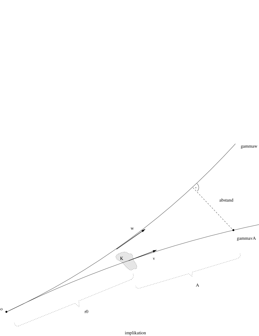
Figure 8:

Corollary 5.8

Let $K\subset UX$ be a $\Gamma$-compact subset consisting only of rank one vectors. Given a shrinking factor $N\in\mathbb{N}$, a shield radius $\Delta>0$ and a radius $r_{0}>0$ there is a distance $A>0$ such that the following holds for any $\epsilon<\Delta$:
For any point $o\in X$ and any radial vectors $v\in K$ and $w\in UX$ with origin $o$ and $d(p(v),o)\geq r_{0}$ the inequality $d(\gamma_{v}(A),\gamma_{w})\leq\epsilon$ implies that $d^{1}(v,\dot{\gamma}_{w})<\epsilon/N$ holds.

6 Avoiding a Rank One Vector

This section explains the construction of Sergei Buyalo and Viktor Schroeder in [whoknows]. They proved that for any given vector $v_{0}\in UM$ of rank one on a compact manifold $M$ of nonpositive curvature and of dimension $\geq 3$ it is possible to construct a closed, flow invariant, full subset $Z\subset UM$ which does not contain $v_{0}$. Furthermore, for every $\epsilon>0$ there is such a set $Z_{\epsilon}$ which is $\epsilon$-dense in $UM$.
The obvious way to construct this set, is to fix some small $\eta>0$ and define

$$Z:=\left\{v\in UM\;|\;d(\dot{\gamma}_{v},v_{0})\geq\eta\right\}$$

but for all we know, this set could be empty or neither full nor $\epsilon$-dense. So how do we prove that this set is full, provided $\eta$ is small enough?
Pick any point $o\in M$ and show that, for $\eta$ small enough, we can find many geodesics passing through $o$ and avoiding an $\eta$-neighbourhood of $v_{0}$. These geodesics can be explicitly constructed.

6.1 Idea

Consider a compact connected manifold $M$ of nonpositive curvature, a rank one vector $v_{0}\in UM$ and a point $o\in M$. Let $\pi:X\rightarrow M$ be the universal covering and choose one element in $\pi^{-1}(o)$ which we will identify with $o$.
We want to find a geodesic in $M$ that avoids the direction $v_{0}$ in the unit tangent bundle of $M$. In the universal covering this corresponds to avoiding the set $\Omega:=d\pi^{-1}(v_{0})\subset UX$. We can identify this set with the set of its base points $\Sigma:=p(d\pi^{-1}(v_{0}))=\pi^{-1}(p(v_{0}))$ via the base point projection. Elements of $\Sigma$ will be denoted with $\omega$ and the corresponding vector in $\Omega$ with $v_{\omega}$. Thus $p(v_{\omega})=\omega$. For technical reasons in Proposition 6.5 we would like $\Omega$ to be symmetric. Hence suppose that $\pm v_{\omega}\in\Omega$ holds for all $\omega\in\Sigma$.
Obviously, a geodesic that avoids some neighbourhood of an $\omega$, avoids an even bigger neighbourhood of the vector $v_{\omega}$. ($d(\gamma,\omega)>\eta\Rightarrow d(\dot{\gamma},v_{\omega})>\eta$). Hence we will work in $X$ rather than in $UX$ and try to avoid $\Sigma$. But indeed we only need to consider elements of $\Sigma$ which correspond to vectors $v_{\omega}$ which are almost radial with respect to our starting point $o$. So for small $\tilde{\epsilon}>0$ ($\tilde{\epsilon}$ will be specified later on) we define the subsets

$$\Sigma(o,\tilde{\epsilon}):=\left\{\omega\in\Sigma\;|\;d\left(v_{\omega},\phi_{\mathbb{R}_{+}}(U_{o}X)\right)<\tilde{\epsilon}\right\}$$

To every $\omega\in\Sigma(o,\tilde{\epsilon})$ we now assign a region in $X$ that should not be hit (the protective disk) and a region that is save to hit (the good annulus) and a sphere inside this annulus that is far away from the boundary of the annulus (the good sphere).

A ray originating in $o$ that comes close to an obstacle $\omega\in\Sigma(o,\tilde{\epsilon})$ will be replaced by a close ray passing the good sphere.

Proposition 6.1 will show that for small displacements it holds: If the new ray hits another protective screen $D_{\omega^{\prime}}$ then any ray hitting the new annulus $R_{\omega^{\prime}}$ will have passed through the old annulus $R_{\omega}$ before. This is illustrated in Figure 9.

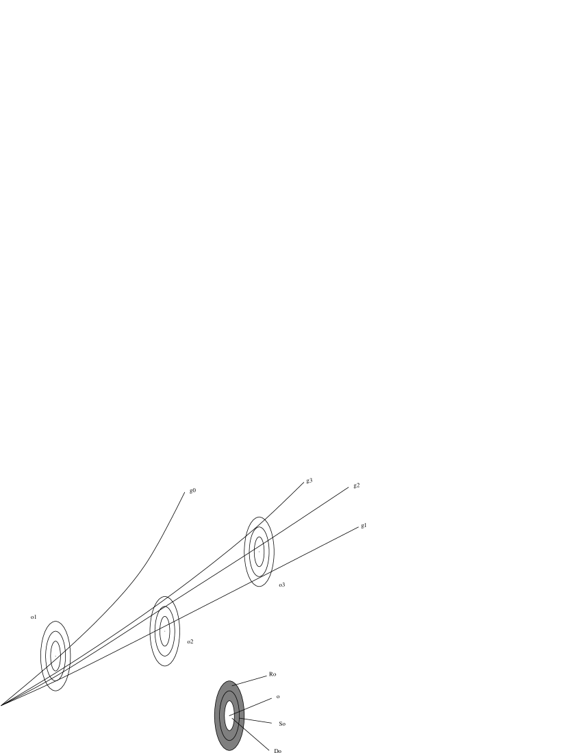
Figure 9: How to Avoid Obstacles

Definition 6.1

For $v\in U_{o}X$ and $\omega\in\Sigma(o,\tilde{\epsilon})$ define $p(\omega,v)$, to be the point of minimal distance to $\omega$ on the ray $\gamma_{v}([0,\infty[)$. For this distance we write $d_{\omega}(v):=d(p(\omega,v),\omega)=d(\gamma_{v},\omega)$.

Consider a small $\delta^{\prime}$ (it will be specified later on). Choose a $\delta<\delta^{\prime}/6$ and define for every $\omega\in\Sigma(o,\tilde{\epsilon})$ the protective screen (disk)

$$D_{\omega}:=\{p(\omega,v)|v\in U_{o}X\text{ und }d_{\omega}(v)<2\delta\},$$

the good annulus

$$R_{\omega}:=\{p(\omega,v)|v\in U_{o}X\text{ und }d_{\omega}(v)\in]\delta,3\delta[\}$$

and contained in the good annulus, the good sphere

$$S_{\omega}:=\{p(\omega,v)|v\in U_{o}X\text{ und }d_{\omega}(v)=2\delta\}.$$

6.2 Choice of Constants

Choose a neighbourhood ${\cal U}_{0}$ of $v_{0}$ such that it consists of rank one vectors only and such that its inverse image under $d\pi$ consists of disjoint sets ${\cal U}_{\omega}$. Choosing the neighbourhood small enough, we can suppose that it is contained in a compact set with the same properties. The preimage of this set under $d\pi^{-1}$ is a $\Gamma$-compact set in $UX$. For this $\Gamma$-compact set and $N=6$ Proposition 5.3 yields constants $\delta^{\prime},a$ where we may assume that $\delta^{\prime}<a/2$. We deduce that the property in Proposition 5.3 holds for the subset $d\pi^{-1}{\cal U}_{0}$ with the same constants $\delta^{\prime},a,N=6$.

In fact we want $\delta^{\prime}$ to satisfy two further conditions.

1. Since ${\cal U}_{0}$ is open, we can find an $\eta>0$ such that ${\cal W}_{\eta}(v_{0})\subset{\cal U}_{0}$ and thus ${\cal W}_{\eta}(v_{\omega})\subset{\cal U}_{\omega}$ for all $\omega$.
   By Lemma 4.2 we may suppose that $\delta^{\prime}$ was chosen so small that, if we put $\delta:=\delta^{\prime}/6$, for any $\omega\in\Sigma(o,\tilde{\epsilon})$ satisfying $d(\omega,o)\geq a$ all the radial rays originating in $o$ and hitting the protective disk or the good annulus of $\omega$ are within $\eta$-distance of $v_{\omega}$ and therefore are in ${\cal U}_{\omega}$ and of rank one.
   So from now on assume, that for $d(o,\omega)>a$, all radial vectors with origin $o$ hitting $D_{\omega}$ or $R_{\omega}$ are rank one vectors which have the property described in Proposition 5.3.
   

2. Now consider $\Omega_{a}:=\Sigma(o,\tilde{\epsilon})\cap{\cal U}_{a}(o)$. This is the finite set of points in $\Sigma(o,\tilde{\epsilon})$ that are within distance less than $a$ of our starting point $o$. For every $\omega\in\Omega_{a}$ call $\theta_{\omega}\in U_{o}X$ the starting direction of the geodesic ray from $o$ to $\omega$; and for $\eta>0$ define

   $$V_{\eta}(\omega):=\{v\in U_{o}X\,|\,{d}(v_{\omega},\dot{\gamma}_{v}(\mathbb{R}_{+}))<\eta\}.$$

   This is an open subset of $U_{o}X$ and $\operatorname{diam}V_{\eta}(\omega)\overset{\eta\rightarrow 0}{\longrightarrow}0$. Choose $\rho<\underset{\omega_{1},\omega_{2}\in\Omega_{a}}{\min}{d}(\theta_{\omega_{1}},\theta_{\omega_{2}})$ and find an $\eta>0$ so small that $\operatorname{diam}V_{\eta}(\omega)<\rho/5$ for all $\omega\in\Omega_{a}$. Now the sets

   $$U_{1} :=\{v\in U_{o}X\big{|}{d}(v,\theta_{\omega})<\frac{1}{5}\rho\text{ for all }\omega\in\Omega_{a}\}\text{ and }$$

   $$U_{2} :=\{v\in U_{o}X\big{|}{d}(v,\theta_{\omega})<\frac{2}{5}\rho\text{ for all }\omega\in\Omega_{a}\}$$

   have the following properties:

   1. $\{\theta_{\omega}\}_{\omega\in\Omega_{a}}\subset U_{1}\subset U_{2}$

   2. $v\in U_{o}X\backslash U_{1}\quad\Rightarrow\quad{d}(v_{\omega},\dot{\gamma}_{v}(\mathbb{R}_{+}))\geq\eta$ for all $\omega\in\Omega_{a}$

   3. $U_{o}X\backslash U_{2}$ is closed and a sphere with finitely many holes of diameter $\frac{4}{5}\rho$.

   Now choose $\delta^{\prime}<a\sin\frac{\rho}{10}$.

6.3 Construction

Start with a vector $x_{0}\in U_{o}X\backslash U_{2}$. Consider the geodesic ray $\gamma_{x_{0}}([a,\infty[)$. Call $\omega_{1}\in\Sigma(a,\tilde{\epsilon})$ the first obstacle with $d_{\omega_{1}}(x_{0})<2\delta$. Move $x_{0}$ to a vector $x_{1}\in U_{o}X$ with $p(\omega_{1},x_{1})\in S_{\omega_{1}}$, i. e. the geodesic ray $\gamma_{x_{1}}$ passes through the good sphere of $\omega_{1}$.
Now define recursively a sequence of vectors $x_{i}\in U_{o}X$ and elements $\omega_{i}\in\Sigma(o,\tilde{\epsilon})$ as follows: The first time $\gamma_{x_{i}}([d(p(\omega_{i},x_{i}),o,\infty[)$ hits the protective disk of an element of $\Sigma(o,\tilde{\epsilon})$, call this element $\omega_{i+1}$ and move $x_{i}$ to a vector $x_{i+1}\in U_{o}X$ where $\gamma_{x_{i+1}}$ passes the good sphere of $\omega_{i+1}$. We get a sequence $\{x_{i}\}$ of vectors in $U_{o}X$ with the following properties.

1. $d(\omega_{i},\gamma_{x_{i}})=d(\omega_{i},p(\omega_{i},x_{i}))=2\delta$

2. $d(\omega_{i+1},\gamma_{x_{i}})=d(\omega_{i+1},p(\omega_{i+1},x_{i}))<2\delta$

3. $d(\omega_{i+1},\omega_{i})>a+\delta^{\prime}$

4. $d(\omega_{i},o)\geq i\frac{a}{2}$.

6.4 The Construction Has the Desired Properties

We need another technical definition:

Definition 6.2

A subset $\Sigma\subset X$ is called radially $(a,\delta)$-separated with respect to $o\in X$, if for any vector $v\in U_{o}X$ and any two points $\omega_{1},\omega_{2}\in\Sigma$

$$\max\left\{d(\gamma_{v},\omega_{1}),d(\gamma_{v},\omega_{2})\right\}\leq\delta\quad\Longrightarrow\quad d(\omega_{1},\omega_{2})>a.$$

In [whoknows, Lemma 4.3] it is proved for our setting, that if $\gamma_{v_{0}}$ is nonperiodic then for any $a>0$ we can find $\delta$ and $\tilde{\epsilon}$ small enough such that $\Sigma(o,\tilde{\epsilon})$ is radially $(a+\delta,\delta)$-separated for all $o\in X$.
If $\gamma_{v_{0}}$ is periodic of period smaller than $a$, the construction is more difficult. But still we can find a radially separated set $\Sigma^{N}(o,\tilde{\epsilon})$ if we consider the set $\Omega^{N}$ instead of $\Omega$ (consider only every $N^{\text{th}}$ element of $\Omega$ along any geodesic $\gamma_{v_{\omega}}$. For more details see [whoknows]). For the next few pages we will suppose that $\Sigma(o,\tilde{\epsilon})$ is radially separated, but we will return to the problem of $\Sigma^{N}(o,\tilde{\epsilon})$ at the end ot this section.

Notice that the geodesic ray $\gamma_{x_{j}}$ passes through all the good annuli of the $\omega_{i}$ for $i<j$. This is proved in a slightly more general form in the following proposition.

Proposition 6.1

Suppose $\Sigma(o,\tilde{\epsilon})$ is radially $(a+\delta^{\prime},\delta^{\prime})$-separated with respect to $o$. Choose $\delta<\delta^{\prime}/6$. Let $\omega\in\Sigma(o,\tilde{\epsilon})$ and let $v\in U_{o}X$ denote the initial direction of a geodesic ray, hitting the good sphere $S_{\omega}$ in $p(\omega,v)$. Call $\omega^{\prime}\in\Sigma(o,\tilde{\epsilon})$ the first obstacle with $d(\omega^{\prime},o)>d(\omega,o)$ for which the ray hits the protective disk $D_{\omega^{\prime}}$ (i. e. $d_{\omega^{\prime}}(v)<2\delta$). Then:

Any ray that meets the annulus $R_{\omega^{\prime}}$ has passed the annulus $R_{\omega}$ before.
Phrased differently this means for any $x\in U_{o}X$ the following implication holds:

$$\delta<d_{\omega^{\prime}}(x)<3\delta\qquad\Longrightarrow\qquad\delta<d_{\omega}(x)<3\delta$$

Proof of Proposition 6.1: We know $d(p(\omega,v),\omega)=2\delta<\delta^{\prime}$ and $d(p(\omega^{\prime},v),\omega^{\prime})<2\delta<\delta^{\prime}$. Applying the $(a+\delta^{\prime},\delta^{\prime})$-separatedness $d(\omega,\omega^{\prime})>a+\delta^{\prime}$ and thus

$$d(p(\omega^{\prime},v),p(\omega,v))\geq d(\omega,\omega^{\prime})-d(\omega,p(\omega,v))-d(\omega^{\prime},p(\omega^{\prime},v))\geq a+\delta^{\prime}-2\delta-2\delta\geq a.$$

For a vector $x\in U_{o}X$ with $d(p(\omega^{\prime},x),\omega^{\prime})<3\delta$ it follows $d(p(\omega^{\prime},v),\gamma_{x})\leq d(p(\omega^{\prime},x),p(\omega^{\prime},v))<3\delta+2\delta<\delta^{\prime}$. Now Proposition 5.3 can be applied and we find a point $q$ on $\gamma_{x}$ satisfying

$$d(p(\omega,v),q)<\frac{1}{6}d(p(\omega^{\prime},v),p(\omega^{\prime},x))<\frac{1}{6}5\delta=\delta$$

and therefore

$$d(p(\omega,x),\omega)\leq d(q,\omega)\leq d(q,p(\omega,v))+d(p(\omega,v),\omega)<3\delta$$

Suppose now $d(p(\omega,x),\omega)<\delta$. By a similar argument there is a $q^{\prime\prime}$ on $\gamma_{v}$ satisfying $d(p(\omega,x),q^{\prime\prime})<\delta$ and therefore $d(q^{\prime\prime},\omega)<2\delta=d(\gamma_{v},\omega)$ in contradiction to the minimal property of $p(\omega,v)$. $\Box$

The next lemma will show that all the $x_{i}$ respect the minimal distance of $\delta$ to these $\omega$ if $d(\omega_{i},o)>d(\omega,o)$.

Lemma 6.2

For every $\omega\in\Sigma(o,\tilde{\epsilon})$ with $d(\gamma_{x_{i}},\omega)>2\delta$ we have $d(\gamma_{x_{j}},\omega)>\delta$ for all $j>i$.

Proof of Lemma 6.2: Suppose $d(p(\omega,x_{j}),\omega)\leq\delta$. As we know, $\gamma_{x_{j}}$ hits the good annulus of $\omega_{i+1}$. Applying the radial separatedness we get

$$d(p(\omega,x_{j}),p(\omega_{i+1},x_{j})) \geq d(\omega,\omega_{i+1})-d(\omega,p(\omega,x_{j}))-d(\omega_{i+1},p(\omega_{i+1},x_{j}))$$

$$\geq a+\delta^{\prime}-\delta-3\delta>a.$$

Thus there is a $q$ on $\gamma_{x_{i}}$ such that

$$d(q,p(\omega,x_{j}))\leq\frac{1}{6}d(p(\omega_{i+1},x_{j}),p(\omega_{i+1},x_{i}))\leq\frac{5}{6}\delta<\delta,$$

hence $d(\gamma_{x_{i}},\omega)\leq d(q,\omega)<\delta+\delta=2\delta$, a contradiction. $\Box$

Now we have found a sequence of geodesic rays avoiding more and more obstacles. In fact this sequence converges to a geodesic ray avoiding all the obstacles:

Lemma 6.3

For every vector $x_{0}\in U_{o}X\backslash U_{2}$ the sequence $\{x_{i}\}_{i\in\mathbb{N}}$ converges to a vector $z\in U_{o}X\backslash U_{1}$.

Proof of Lemma 6.3: Suppose the sequence is not finite. We know for $j\geq i\geq 1$ that $d(\omega_{i},\gamma_{x_{j}})<3\delta$ since $\gamma_{x_{j}}$ passes the good annulus of $\omega_{i}$. Since $d(\omega_{i},o)>i\frac{a}{2}$ and the angle $\measuredangle(o,p(\omega_{i},x_{j}),\omega_{i})$ is $\frac{\pi}{2}$, we know

$$\sin(\measuredangle(\theta_{\omega_{i}},x_{j}))\leq\frac{3\delta}{i\frac{a}{2}}=\frac{6\delta}{ia}\overset{i\rightarrow\infty}{\longrightarrow}0$$

and thus $\{x_{j}\}$ is a Cauchy sequence converging to a vector $z\in U_{o}X$. Notice that

$$\measuredangle(\theta_{\omega_{1}},z)=\underset{j\rightarrow\infty}{\lim}\measuredangle(\theta_{\omega_{1}},x_{j})\leq\arcsin\left(\frac{6\delta}{a}\right)<\frac{\rho}{10}$$

and since $\gamma_{x_{0}}$ hits the protective disk we know

$$\measuredangle(\theta_{\omega_{1}},x_{0})\leq\arcsin\left(\frac{2\delta}{\frac{a}{2}}\right)<\frac{\rho}{10}.$$

Hence $z$ is within $\frac{\rho}{5}$-distance of $x_{0}$ and therefore in $U_{o}X\backslash U_{1}$. $\Box$

So, by mapping $x_{0}$ to $z$, we can define a map

$$\Phi:U_{o}X\backslash U_{2}\longrightarrow U_{o}X\backslash U_{1}$$

where every vector $z=\Phi(x_{0})$ in the image of $\Phi$ satisfies:

1. The speed vectors $\dot{\gamma}_{z}$ of the geodesic ray $\gamma_{z}$ respect a distance of $\tilde{\epsilon}$ (with respect to ${d}(.,.)$) to all $v_{\omega}$ with $\omega\in\Sigma\backslash\Sigma(o,\tilde{\epsilon})$.

2. The geodesic ray $\gamma_{z}$ respects a distance of $\delta$ to all $\omega\in\Sigma(o,\tilde{\epsilon})\backslash\Omega_{a}$.

3. The geodesic ray $\gamma_{z}$ respects a distance of $\eta$ to all $\omega\in\Omega_{a}$.

Furthermore $\Phi$ satisfies

$$d(x_{0},\Phi(x_{0}))<\frac{\rho}{5}\text{ for all }x_{0}\in U_{o}X\backslash U_{2}.$$

Notice that we can choose $\rho$ arbitrarily small and still find appropriate $\eta$, $\delta<\delta^{\prime}/6$ and $\tilde{\epsilon}$.

Lemma 6.4

Fix $\rho>0$. For any submanifold $Y\subset U_{o}X\backslash U_{2}$ we can define a continuous map

$$\Phi_{Y}:Y\rightarrow U_{o}X\backslash U_{1}$$

and an $\eta>0$ such that the image $\Phi_{Y}(Y)$ consists of initial directions of geodesic rays that miss the neighbourhood $\underset{\omega\in\Omega}{\bigcup}{\cal W}_{\eta}(v_{\omega})$ of $\Omega$ and such that

$${d}(\Phi_{Y}(y),y)<\frac{\rho}{5}\text{ for all }y\in Y.$$

Proof of Lemma 6.4: Instead of moving every starting vector individually and looking at the limit we now consider its neighbourhood in $Y$. So consider an obstacle $\omega$. Notice that $\gamma_{Y}\cap D_{\omega}$ is an at most $\dim Y$-dimensional submanifold of $D_{\omega}$ which may therefore be deformed continuously into $S_{\omega}$ keeping $\gamma_{Y}\cap S_{\omega}$ fixed. This deformation in $\gamma_{Y}\cap D_{\omega}$ can be projected down to $U_{o}X$ and we get a series of deformations of $Y$ with a continuous limit deformation $\Phi_{Y}$. $\Box$

Now we are in the position to prove our main proposition:

Proposition 6.5

If $M$ is a compact manifold of nonpositive curvature and $v_{0}\in UM$ is a vector of rank one, then for any $o\in M$ we can find a geodesic $\gamma:\mathbb{R}\rightarrow M$ and an open neighbourhood $\cal U$ of $v_{0}$ in $UM$ such that $\gamma(0)=o$ and $\gamma$ does not meet $\cal U$.

Proof of Proposition 6.5: Of course we work in the universal covering $X$ of $M$ as before. Use all the notations as introduced in this section.
Fix one vector $S\in U_{o}X\backslash U_{2}$, the south-pole. Take a $\dim(X)-2$-dimensional subspace $W$ of $T_{S}U_{o}X$ and its one dimensional orthogonal complement $W^{\perp}$. Define two submanifolds of $U_{o}X$ of dimensions $\dim(X)-2$ and $1$ respectively by $Y:=\exp_{S}W$ and $Y^{\perp}:=\exp_{S}W^{\perp}$. Because $U_{o}X\backslash U_{2}$ looks like a sphere with small holes of diameter $\frac{2}{5}\rho$, we can choose a deformation $\phi:U_{o}X\rightarrow U_{o}X$ that deforms $Y$ and $-Y^{\perp}$ into two submanifolds $Y_{1}$ and $-Y_{1}^{\perp}$ of $U_{o}X\backslash U_{2}$ and every point of $U_{o}X$ is moved by at most $\frac{2}{5}\rho$.
Now apply Lemma 6.4 to $Y_{1}$ and $-Y_{1}^{\perp}$ and deform them into simplices in $U_{o}X$ homotopic to $Y$ and $-Y^{\perp}$, respectively. Notice that $\Phi_{Y_{1}}\circ\phi$ and $\Phi_{-Y^{\perp}_{1}}\circ\phi$ move every vector by less than $\frac{3}{5}\rho$. Since $Y$ and $Y^{\perp}$ intersect in two antipodal points and the intersection number of homotopic simplices is a constant, $\Phi_{Y_{1}}(\phi(Y))$ and $-\Phi_{-Y_{1}^{\perp}}(\phi(-Y^{\perp}))$ still intersect in two points, provided $\frac{6}{5}\rho<\pi$.
Take one of these intersection points $z$. Since $z\in\Phi_{Y_{1}}(\phi(Y))$ we know that $\gamma_{z}(\mathbb{R}_{+})$ avoids a neighbourhood of $v_{0}$ and since $-z\in\Phi_{-Y_{1}^{\perp}}(\phi(-Y))$ so does $\gamma_{z}(\mathbb{R}_{-})$. $\Box$

Remark 6.1

• In fact all the constants were chosen globally. So all the geodesic we constructed avoid the same neighbourhood of $v_{0}$. So the set

  $$Z:=\left\{v\in UM\;|\;d(\dot{\gamma}_{v},\Omega)\geq\eta\right\}$$

  is full.

• Take a closer look at the proof of Proposition 6.5: Given any vector $v\in U_{o}X$ there is a vector $S\in U_{o}X\backslash{\cal U}_{2}$ that is at most $(\frac{2}{5}\rho)$-far from $v$. The construction yields a vector $v^{\prime}$ such that $\dot{\gamma}_{v^{\prime}}$ avoids an $\eta$-neighbourhood of $\Omega$ and $v^{\prime}$ is $(\frac{6}{5}\rho)$-close to $S$. Thus $Z$

  is $(\frac{8}{5}\rho)$-dense in $UM$.

• As remarked before, if $\gamma_{v_{0}}$ is $L$-periodic we have to modify the proof. Proposition 6.5 holds for $\Sigma^{N}(o,\tilde{\epsilon})$ instead of $\Sigma(o,\tilde{\epsilon})$. Now suppose $\dot{\gamma}_{v}$ avoids an $\eta$-neighbourhood of $\Omega^{N}$. But if $\gamma_{v}$ came very close, say $\nu$, to $v_{\omega}\in\Omega$ then it would be close to $\gamma_{v_{\omega}}$ for a long time, say $T$. But if this time is much bigger than $N$ times the period of $\gamma_{v_{0}}$ then it would pass at least one of the obstacles in $\Omega^{N}$very closely. Therefore $\nu$ can not be arbitrarily small and Proposition 6.5 holds for periodic $v_{0}$, too.

7 Avoiding Subsets of Small s-Dimension

Consider a Riemannian manifold $X$ and a closed submanifold $R\subset X$ of smaller dimension $\dim(R)<\dim(X)$. In this section we discuss deformations of $UX\backslash UR$ such that every vector is moved away from $UR$.
$UR$ is a submanifold of the Riemannian manifold $UX$. So if there is a $2\epsilon$-neighbourhood ${\cal W}_{2\epsilon}(UR)$ of $UR$ on which the gradient $\operatorname{grad}d_{UR}$ of the distance function $d_{UR}:=d(UR,.)$ is defined, we can use the flow $\phi$ generated by $\operatorname{grad}d_{UR}$ to deform $UX\backslash UR$ into $UX\backslash{\cal W}_{\epsilon}(UR)$. Notice that the gradient and hence $\phi$ might not be defined outside ${\cal W}_{2\epsilon}(UR)$ but still the deformation

$$\Phi(v):=\phi_{\max\{0,2\epsilon-\frac{1}{2}d_{UR}(v)\}}(v)$$

is well defined and moves every vector by at most $2\epsilon$ into $UX\backslash{\cal W}_{\epsilon}(UR)$.

We need, however, a more elaborated deformation, since it will be essential for us to have control on the displacement of the base points, too. Furthermore we want our deformation to respect the foliation of $UX$ into spheres ${\cal S}_{v}(r)$ of fixed radius $r$.
In Subsection 7.1 we will discuss a deformation which gives control on $d_{UR}$ and on the base point distance from $R$ at the same time. Based on this deformation we will find another deformation in Subsection 7.2 that respects the sphere foliation of $UX$.
Finally in Corollary 7.8 we generalize the deformation to the case where $R$ is a stratified subset of $X$:

Corollary 7.8

Let $X$ denote a Hadamard manifold with compact quotient $M=X/\Gamma$. Suppose a $\Gamma$-compact stratified subset $R\subset X$ and $r_{0}>0$ are given.

Then there is a constant $k>0$ such that for small $\lambda>0$ and given $r>r_{0}$, $v\in UX$ and manifold $Y$ with

$$\dim Y<\dim X-\dim R$$

we can deform any continuous map $c:Y\rightarrow{\cal S}_{r}(v)$ into a continuous map $c_{\lambda}:Y\rightarrow{\cal S}_{r}(v)$ such that $c_{\lambda}$ is $k\lambda$-close to $c$ and $c_{\lambda}$ avoids a $\lambda$-neighbourhood of $UR$, i. e. for all $x\in Y$

$$d(c(x),c_{\lambda}(x))\leq k\lambda\qquad\text{ and }\qquad d_{UR}(c_{\lambda}(x))\geq\lambda.$$

7.1 Avoiding the Unit Tangent Bundle of a Submanifold

Suppose $X$ is a Hadamard manifold with compact quotient $M=X/\Gamma$ and $R\subset X$ is a $\Gamma$-compact submanifold of $X$. We will try to avoid its unit tangent bundle $UR$ in $UX$. Use the shorthand notation $d_{R}(.):=d(R,.)$ for the distance to $R$ in $X$ and $d_{UR}:=d(UR,.)$ for the distance in $UX$ to $UR$.

If $R$ is a submanifold with boundary, notice that we can find a slightly larger, $\Gamma$-compact submanifold $R^{\prime}$ in $X$ with $\dim R^{\prime}=\dim R$, $R\subset R^{\prime}$ and $d(R,\partial R^{\prime})>\rho$ for some $\rho>0$. If $R$ is a closed manifold without boundary, set $R^{\prime}=R$. The proof still works.
Suppose furthermore that $\rho>0$ is so small that

• $\rho$ is smaller than the injectivity radius of $M$

• $\rho$ is smaller than the injectivity radius of $UM$

• $\rho$ is so small that $\operatorname{grad}_{p}d_{R^{\prime}}$ is defined for all $p\in X$ with $0<d_{R^{\prime}}(p)<\rho$.
  Hence $\gamma_{p}:=\gamma_{\operatorname{grad}_{p}d_{R^{\prime}}}$ realizes the distance from ${R^{\prime}}$ to $\gamma_{p}(t)$ for all $t\in[-d_{R^{\prime}}(p),\rho-d_{R^{\prime}}(p)]$.

Fix $\epsilon<\rho$.
We define the distortion $\Pi_{\epsilon}$ of $UX\backslash p^{-1}{R^{\prime}}:=\{v\in UX\;\big{|}\;p(v)\notin{R^{\prime}}\}$. To shorten notation we define the distortion length (depending on $\epsilon$)

$$\begin{array}[]{ccccc}\alpha:&UX\backslash p^{-1}{R^{\prime}}&\longrightarrow&[0,2\epsilon]\\ &v&\longmapsto&\begin{array}[]{\{}{c}.0\\ 2\epsilon-\frac{1}{2}{d_{U{R^{\prime}}}(v)}\end{array}&\begin{array}[]{c}\text{ if }d_{U{R^{\prime}}}(v)\geq 4\epsilon\\ \text{ if }d_{U{R^{\prime}}}(v)\leq 4\epsilon.\end{array}\end{array}$$

The distortion is defined by

$$\begin{array}[]{cccc}\Pi_{\epsilon}:&UX\backslash p^{-1}{R^{\prime}}&\longrightarrow&UX\backslash p^{-1}{R^{\prime}}\\ &v&\longmapsto&{}_{\gamma_{p(v)}}\big{\|}_{0}^{\alpha(v)}v.\end{array}$$

This is well defined, since $\alpha(v)=0$ for those $v$ where the gradient of $d_{R^{\prime}}$ is not defined in $p(v)$.

Proposition 7.1

The distortion $\Pi_{\epsilon}$ has the following properties if we choose $\epsilon<\frac{\rho}{4}$:

1. $d(v,\Pi_{\epsilon}(v))=\alpha(v)$ for all $v\in UX\backslash p^{-1}{R^{\prime}}$.
   Furthermore $d(v,_{\gamma_{p(v)}}\big{\|}_{0}^{t}v)=t$ for all $t\in[0,\alpha(t)]$.

2. $d_{R^{\prime}}(p(\Pi_{\epsilon}(v)))=d_{R^{\prime}}(p(v))+\alpha(v)>0$ for all $v\in UX\backslash p^{-1}{R^{\prime}}$.
   Furthermore $\gamma_{p(v)}$ is a shortest from ${R^{\prime}}$ to $\gamma_{p(v)}(t)$ for all $t\in[0,\alpha(t)]$.

3. For all $v\in UX\backslash p^{-1}{R^{\prime}}$ we have

   $$\begin{array}[]{ccccc}d_{U{R^{\prime}}}(v)\geq 4\epsilon&\Longleftrightarrow&d_{U{R^{\prime}}}(\Pi_{\epsilon}(v))\geq 4\epsilon&\Longleftrightarrow&\Pi_{\epsilon}(v)=v\\ d_{U{R^{\prime}}}(v)<4\epsilon&\Longleftrightarrow&d_{U{R^{\prime}}}(\Pi_{\epsilon}(v))<4\epsilon.\end{array}$$

4. $\Pi_{\epsilon}$ is continuous, injective and a homeomorphism onto the image.

5. The image of $\Pi_{\epsilon}$ is contained in $UX\backslash{\cal W}_{\epsilon}U{R^{\prime}}$,
   i. e. $d_{U{R^{\prime}}}(\Pi_{\epsilon}(v))\geq\epsilon$ for all $v\in UX\backslash p^{-1}{R^{\prime}}$.

6. $\Pi_{\epsilon}$ is compatible with the $\Gamma$-action on $X$ and $UX$.

Proof of Proposition 7.1: Recall that for any $v\in UX\backslash p^{-1}{R^{\prime}}$ the curve

$$\sigma_{v}:t\longmapsto_{\gamma_{p(v)}}\big{\|}_{0}^{t}v$$

is a geodesic in $UX$. Since the projection $p\circ\sigma_{v}=\gamma_{p(v)}$ is a shortest from ${R^{\prime}}$ to $\gamma_{p(v)}(t)$ for $t\in]-d_{R^{\prime}}(p(v)),\rho-d_{R^{\prime}}(p(v))]$ it does not intersect ${R^{\prime}}$ and hence $\sigma_{v}(t)\notin U{R^{\prime}}$ for these $t$.
We conclude that $\phi_{v}:t\mapsto d_{U{R^{\prime}}}(\sigma_{v}(t))$ is differentiable for these $t$ and $\phi_{v}^{\prime}(t)\in[-1,1]$.

1. This holds since $\sigma_{v}$ is a geodesic and $\alpha(v)$ is smaller than the injectivity radius of $UX$.

2. $\gamma_{p(v)}$ realises the distance to ${R^{\prime}}$ for $t-d_{R^{\prime}}(p(v))<\rho$. Since $p(\Pi_{\epsilon}(v))=p(_{\gamma_{p(v)}}\big{\|}_{0}^{\alpha(v)}v)=\gamma_{p(v)}(\alpha(v))$ we get $d_{R^{\prime}}(p(\Pi_{\epsilon}(v)))=d_{R^{\prime}}(p(v))+\alpha(v)$.

3. The implications

   $$\Pi_{\epsilon}(v)=v\;\;\Longleftarrow\;\;d_{U{R^{\prime}}}(v)\geq 4\epsilon\;\;\Longrightarrow\;\;d_{U{R^{\prime}}}(\Pi_{\epsilon}(v))\geq 4\epsilon$$

   are obvious. We need to show

   $$d_{U{R^{\prime}}}(v)<4\epsilon\;\;\Longrightarrow\;\;d_{U{R^{\prime}}}(\Pi_{\epsilon}(v))<4\epsilon.$$

   So take $v\in UX\backslash p^{-1}{R^{\prime}}$ with $d_{U{R^{\prime}}}(v)<4\epsilon$. Then

   $$d_{U{R^{\prime}}}(\Pi_{\epsilon}(v)) \leq d_{U{R^{\prime}}}(v)+d(v,\Pi_{\epsilon}(v))$$

   $$=d_{U{R^{\prime}}}(v)+\alpha(v)$$

   $$=2\epsilon+\frac{1}{2}\underset{<4\epsilon}{\underbrace{d_{U{R^{\prime}}}(v)}}<4\epsilon.$$

4. $\Pi_{\epsilon}$ is continuous since $\alpha$ is.
   Suppose we find $v_{1},v_{2}\in UX\backslash p^{-1}{R^{\prime}}$ with $z:=\Pi_{\epsilon}(v_{1})=\Pi_{\epsilon}(v_{2})$.
   

   • Suppose $d_{U{R^{\prime}}}(z)\geq 4\epsilon$ and therefore $d_{U{R^{\prime}}}(v_{1}),d_{U{R^{\prime}}}(v_{2})\geq 4\epsilon$. But $v_{1}=\Pi_{\epsilon}(v_{1})=z=\Pi_{\epsilon}(v_{1})=v_{2}$ for these vectors.

   • Now suppose $d_{U{R^{\prime}}}(z)<4\epsilon$ and hence $d_{U{R^{\prime}}}(v_{i})<4\epsilon$ for both $i$ and $\alpha(v_{i})=2\epsilon-\frac{1}{2}d_{U{R^{\prime}}}(v_{i})$.
     We use the notation $p_{i}:=p(v_{i})$, $\gamma_{i}:=\gamma_{p_{i}}$, $\sigma_{i}:=\sigma_{v_{i}}$, $\phi_{i}:=\phi_{v_{i}}$.
     Without loss of generality we suppose

     $$d_{R^{\prime}}(p_{1})\leq d_{R^{\prime}}(p_{2}).$$ (6)

     By Part 2 of the proposition

     $$d_{R^{\prime}}(p_{1})+\alpha(v_{1})=d_{R^{\prime}}(z)=d_{R^{\prime}}(p_{2})+\alpha(v_{2})$$ (7)

     and by condition (6) $\alpha(v_{1})-\alpha(v_{2})=d_{R^{\prime}}(p_{2})-d_{R^{\prime}}(p_{1})\geq 0$ which translates into

     $$d_{U{R^{\prime}}}(v_{1})\leq d_{U{R^{\prime}}}(v_{2}).$$ (8)

     By definition of $\Pi_{\epsilon}$ the points $p_{i}$ and $q:=p(z)$ lie on the unique shortest geodesic from ${R^{\prime}}$ to $q$. And the vectors $v_{i}$ and $z$ can be obtained via parallel transport along that geodesic $\sigma_{1}$. So

     $$\sigma_{1}(0) =v_{1}$$ (9)

     $$\sigma_{1}(d_{R^{\prime}}(p_{2})-d_{R^{\prime}}(p_{1})) =v_{2}$$ (10)

     $$\sigma_{1}(\alpha(v_{1})) =z$$ (11)

     Now recall that $\phi_{1}(t)$ is differentiable for $t\in[0,\alpha(v_{1})]$ with derivative in $[-1,1]$. Therefore

     $$d_{U{R^{\prime}}}(v_{2})=\phi_{1}(d_{R^{\prime}}(p_{2})-d_{R^{\prime}}(p_{1}))\leq\underset{=d_{U{R^{\prime}}}(v_{1})}{\underbrace{\phi_{1}(0)}}+(d_{R^{\prime}}(p_{2})-d_{R^{\prime}}(p_{1}))$$

     and thence

     $$d_{U{R^{\prime}}}(v_{2})-d_{U{R^{\prime}}}(v_{1})\leq d_{R^{\prime}}(p_{2})-d_{R^{\prime}}(p_{1})\overset{(\ref{alphas})}{=}\alpha(v_{1})-\alpha(v_{2})=\frac{1}{2}(d_{U{R^{\prime}}}(v_{2})-d_{U{R^{\prime}}}(v_{1})).$$

     Combining this with (8) we see that $d_{U{R^{\prime}}}(v_{1})=d_{U{R^{\prime}}}(v_{2})$, hence $\alpha(v_{1})=\alpha(v_{2})$ and by (7) $d_{R^{\prime}}(p_{2})=d_{R^{\prime}}(p_{1})$. By (9) and (10) we get

     $$v_{1}\overset{(\ref{sigma1})}{=}\sigma_{1}(0)=\sigma_{1}(d_{R^{\prime}}(p_{2})-d_{R^{\prime}}(p_{1}))\overset{(\ref{sigma2})}{=}v_{2}.$$

   It remains to show that $\Pi_{\epsilon}^{-1}$ is continuous. Write $Y:=U{R^{\prime}}\backslash p^{-1}{R^{\prime}}$.
   Take any $v\in Y$ and fix $\eta<\frac{1}{2}d_{R^{\prime}}(p(v))$. We claim that $\Pi_{\epsilon}({\cal W}_{\eta}(v))$ is open in $\Pi_{\epsilon}(Y)$.
   Write ${\cal U}$ for ${\cal W}_{\eta}(v)$ and assume that $\Pi_{\epsilon}({\cal U})$ is not open. Then we find a sequence $\Pi_{\epsilon}(v_{i})\in\Pi_{\epsilon}(Y)\backslash\Pi_{\epsilon}({\cal U})=\Pi_{\epsilon}(Y\backslash{\cal U})$ converging to a vector $\Pi_{\epsilon}(w)\in\Pi_{\epsilon}({\cal U})$. But $\{v_{i}\}_{i}$ is a bounded sequence in $Y$ since

   $$d(v_{i},w)\leq\underset{\leq 2\epsilon}{\underbrace{d(v_{i},\Pi_{\epsilon}(v_{i}))}}+\underset{\rightarrow 0}{\underbrace{d(\Pi_{\epsilon}(v_{i}),\Pi_{\epsilon}(w))}}+\underset{\leq 2\epsilon}{\underbrace{d(\Pi_{\epsilon}(w),w)}}$$

   and therefore a subsequence converges to a vector $z\in UX\backslash{\cal U}$ (closed set) whose base point lies not in ${R^{\prime}}$ since

   $$d_{R^{\prime}}(p(z))\leftarrow d_{R^{\prime}}(p(v_{i}))\geq d_{R^{\prime}}(p(v))-\eta>\frac{1}{2}d_{R^{\prime}}(p(v))>0.$$

   So $z\in Y\backslash{\cal U}$ and $\Pi_{\epsilon}(z)=\Pi_{\epsilon}(\lim v_{i})=\lim\Pi_{\epsilon}(v_{i})=\Pi_{\epsilon}(w)$ and by injectivity $w=z$ which is a contradiction since $w\in{\cal U}$ and $z\notin{\cal U}$.

5. Take $v\in UX\backslash p^{-1}{R^{\prime}}$. To see that $d_{U{R^{\prime}}}(\Pi_{\epsilon}(v))>\epsilon$ we need to distinguish three cases:

   • If $d_{U{R^{\prime}}}(v)\geq 4\epsilon$ then $\Pi_{\epsilon}(v)=v$ and $d_{U{R^{\prime}}}(\Pi_{\epsilon}(v))\geq 4\epsilon$.

   • If $d_{U{R^{\prime}}}(v)\leq 2\epsilon$ then

     $$d_{U{R^{\prime}}}(\Pi_{\epsilon}(v)) \geq d_{R^{\prime}}(p(\Pi_{\epsilon}(v)))$$

     $$=d_{R^{\prime}}(p(v))+\alpha(v)$$

     $$>\alpha(v)$$

     $$=2\epsilon-\frac{1}{2}d_{U{R^{\prime}}}(v)\geq\epsilon.$$

   • If $d_{U{R^{\prime}}}(v)>2\epsilon$ then

     $$d_{U{R^{\prime}}}(\Pi_{\epsilon}(v)) \geq d_{U{R^{\prime}}}(v)-d(v,\Pi_{\epsilon}(v))$$

     $$=d_{U{R^{\prime}}}(v)-\alpha(v)$$

     $$=\frac{3}{2}d_{U{R^{\prime}}}(v)-2\epsilon>\epsilon.$$

6. This is obvious since the distance functions and hence the gradient field are invariant under deck transformations.

$\Box$

Remark 7.1

The construction uses a displacement of maximally $2\epsilon$ to achieve a distance to $U{R^{\prime}}$ of at least $\epsilon$. The quotient of these two values is

$$\frac{\text{distance}}{\text{displacement}}\;=\;\frac{1}{2}.$$

Optimal would be a value of $1$ while any value $>0$ might be called satisfactory. A natural approach to maximize the quotient is to consider a different distortion length function. For $\lambda\in]0,2[$ we could use $\alpha_{\lambda}:=\lambda\alpha$ (For $\lambda\geq 2$ the construction would fail to be injective). Then Proposition 7.1 holds for all $\epsilon<\frac{\rho}{2\lambda}$ with maximal displacement $2\lambda\epsilon$ and minimal distance to $U{R^{\prime}}$ at least $\frac{2\lambda}{\lambda+1}\epsilon$. So in this way the quotient is

$$\frac{\text{distance}}{\text{displacement}}\;=\;\frac{1}{\lambda+1}$$

and hence for small $\epsilon$ the distortion becomes very effective.

7.2 Respecting the $r$-Sphere Foliation of $UX$

Next we will use the distortion $\Pi_{\epsilon}$ to define distortions on $UX\backslash p^{-1}R^{\prime}$ that map vectors normal to a sphere to vectors that are normal to the same sphere. This distortion will be denoted by $\Psi_{r,\epsilon}$ where $r$ is the radius of the sphere. We will use the following notation:
For $p\in R^{\prime}\backslash\partial R^{\prime}$ define the normal tangent space by

$${\cal N}_{p}R^{\prime}:=\{u\in T_{p}X\;|\;u\perp v\text{ for all }v\in T_{p}R^{\prime}\}.$$

Notice that $R\subset R^{\prime}\backslash\partial R^{\prime}$ and hence we can define the normal bundle normal bundle ${\cal N}R\subset TX$ of $R$ by

$${\cal N}R:=\underset{p\in R}{\bigcup}{\cal N}_{p}R^{\prime}.$$

This is a proper euclidean bundle over $R$ which is independent of the choice of $R^{\prime}$.

The unit normal bundle is the subset of all vectors of unit length and will be denoted by ${\cal N}^{1}R\subset UX$. This sphere bundle over $R$ is $\Gamma$-compact.

For $r>0$ and $v\in UX$ recall the definition of spheres of radius $r$ defined by $v$

in $X$:

$S_{r}(v):=\{q\in X\;\big{|}\;d(\gamma_{v}(-r),q)=r\}$ and

in $UX$:

${\cal S}_{r}(v):=\{\dot{\sigma}(r)\in UX\;|\;\sigma\text{ geodesic}\wedge\sigma(0)=\gamma_{v}(-r)\wedge\sigma(r)\in S_{r}(v)\}$.

So $S_{r}(v)$ is the sphere of radius $r$ centered at $\gamma_{v}(-r)$ (hence $p(v)\in S_{r}(v)$) and ${\cal S}_{r}(v)$ is the set of outward unit vectors to this sphere (and by construction $v\in{\cal S}_{r}(v)$).
Now fix a radius $r$. We want to define a distortion

$$\Psi_{r,\epsilon}:UX\backslash p^{-1}{R^{\prime}}\longrightarrow UX\text{ such that }\Psi_{r,\epsilon}(v)\in{\cal S}_{r}(v)\text{ for all }v.$$

The idea of the construction is illustrated in figure 10.

Figure 10: Construction of $\Psi_{r,\epsilon}$

For any vector $v$ let $m:=\gamma_{v}(-r)$ denote the centre of the sphere to which $v$ is a normal vector. Write $\sigma$ for the geodesic starting in $m$ and passing through $q:=p(\Pi_{\epsilon}(v))$. Call $q^{\prime}$ the point on $\sigma$ at distance $r$ from $m$, so $p:=p(v)$ and $q^{\prime}$ lie on the sphere around $m$ of radius $r$. Define the vector tangent to $\sigma$ in $q^{\prime}$ to be $\Psi_{r,\epsilon}(v)$. We might as well describe the map by

$$\Psi_{r,\epsilon}(v):=\frac{d}{dt}\Big{|}_{t=r}\exp_{\gamma_{v}(-r)}\left(t\frac{\exp^{-1}_{\gamma_{v}(-r)}(p(\Pi_{\epsilon}(v)))}{\|\exp^{-1}_{\gamma_{v}(-r)}(p(\Pi_{\epsilon}(v)))\|}\right)$$

which shows that the map is surely continuous for $r>2\epsilon\geq\alpha(v)$.
We will see that for small $\epsilon$ and big $r$ this distortion has the property that the displacement is small and still the distance to $UR$ of the image is strictly bigger than zero by Proposition 7.6. To see this we have to consider the behaviour of the following functions first:

Fix a point $p\in X$ and vectors $v,z\in U_{p}X$. For $a\in\mathbb{R}_{+}$ let $\Pi_{\epsilon,a}(v,z):=_{\gamma_{z}}\big{|}_{0}^{a}v$ denote the vector we get by parallel transport of $v$ along the geodesic segment $\gamma_{z}\big{\|}_{[0,a]}$.
For $r\in\mathbb{R}_{+}$ map $v$ to the vector $w_{a,r}(v,z)$ that is tangent in $\gamma_{z}(a)$ to the geodesic $\sigma$ starting in $\gamma_{v}(-r)$ and passing through $\gamma_{z}(a)$. So for fixed $r$ and $v$ the vectors $w_{a,r}(v,z)$ are radial vectors originating in $\gamma_{v}(-r)$ with base point on $\gamma_{z}$.

Write $q_{a}(v,z)$ for the base point $\gamma_{z}(a)$ of $\Pi_{\epsilon,a}(v,z)$ and $w_{a,r}(v,z)$ (notice that $q_{a}(v,z)$ is independent of $r$). The point on the geodesic $\sigma$ that is at distance $r$ from $\gamma_{v}(-r)$ will be denoted by $q^{\prime}_{a,r}(v,z)$. Write $l_{a}(r,v,z)$ for the distance $d(q_{a}(v,z),q^{\prime}_{a,r})$.

We can estimate the displacement of $\Psi_{r,\epsilon}$ if we understand the following displacements:

$$v \rightarrow\Pi_{\epsilon}(v)=\Pi_{\epsilon,\alpha(v)}(v,\operatorname{grad}_{p}d_{R^{\prime}})$$ (Step 1)

$$\rightarrow w_{\alpha(v),r}(v,\operatorname{grad}_{p}d_{R^{\prime}})=:w_{r}(v)$$ (Step 2)

$$\rightarrow\Psi_{r,\epsilon}(v)$$ (Step 3)

By Proposition 7.1 we understand quite well Step 1. We want $\Psi_{r,\epsilon}$ to inherit the main properties of this map. So we need to estimate the other two steps. Step 3 is parallel transport along the geodesic $\sigma$. So the displacement is exactly the distance of the base points $d(q,q^{\prime})=|l_{r}(v)-r|$. The displacement in Step 2 is the angle between the radial vector and the parallely transported vector. We will see that these two displacements can be controlled if we make sure $\alpha(v)$ is small enough.

Lemma 7.2 (Step 2)

Given any $r_{0}>0$ there exists $\mu\geq 0$ such that for every $\nu>0$ there is a length $A>0$ such that for all $a<A$ and $r>r_{0}$

$$d(w_{a,r}(v,z),\Pi_{\epsilon,a}(v,z))<(\mu+\nu)a\quad\text{ for all }v,z\in UX\text{ with }p(v)=p(z).$$

Proof of Lemma 7.2:
Idea: Define

$$\mu:=\frac{1}{r_{0}}+\underset{v,z}{\max}\frac{\partial}{\partial a}\Big{|}_{a=0}d(w_{a,r_{0}}(v,z),\Pi_{\epsilon,a}(v,z)).$$

The first summand times $a$ is less than the angle between the vectors in $p(\Pi_{\epsilon,a}(v,z))$ which are radial to $\gamma_{v}(-r_{0})$ and $\gamma_{v}(-r)$ for $r>r_{0}$. The second obviously is an upper bound for the case $r=r_{0}$. $\Box$

Lemma 7.3 (Step 3)

For every $\nu>0$ and $r_{0}>0$ there is a distance $A>0$ such that for all $a<A$ the following holds:

$$\cos(\measuredangle(v,z))-\nu<\frac{l_{a}(r_{0},v,z)-r_{0}}{a}<\cos(\measuredangle(v,z))+\nu$$

for all $v,z\in UX$ with $p(v)=p(z)$ and $\measuredangle(v,z)\leq\frac{\pi}{2}$.
Furthermore holds

$$0\leq l_{a}(r,v,z)-r<l_{a}(r_{0},v,z)-r_{0}\quad\text{ for }r>r_{0}$$

if $r_{0}>a$.

Proof of Lemma 7.3: For simplicity we suppose that the curvature is bounded by $-1\leq K\leq 0$. This rescaling does not change the result.
In the comparison spaces we can apply the Law of Cosine to get an estimate of $l_{a}(r,v,z)$:

$$l_{a}(r,v,z)^{2} \geq r^{2}+a^{2}-2ra\cos(\pi-\measuredangle(v,z))$$ (Euclidean)

$$\cosh(l_{a}(r,v,z)) \leq\cosh(r)\cosh(a)-\cos(\pi-\measuredangle(v,z))\sinh(r)\sinh(a)$$ (Hyperbolic)

Fix $v,z$ and write $l_{a}(r)$ for one of the estimations

$$l_{a}(r) :=\sqrt{r^{2}+a^{2}+2ra\cos(\measuredangle(v,z))}\qquad\qquad\qquad\text{ or }$$

$$l_{a}(r) :=\operatorname{Arcosh}\left(\cosh(r)\cosh(a)+\cos(\measuredangle(v,z))\sinh(r)\sinh(a)\right).$$

Notice that $l_{a}(r)\geq r$ and

$$l_{a}(r_{0})-r_{0}\;\overset{a\rightarrow 0}{\longrightarrow}\;0.$$

So we can use de l’Hôpital to calculate

$$\underset{a\rightarrow 0}{\lim}\frac{l_{a}(r_{0})-r_{0}}{a}=\frac{\partial}{\partial a}\Big{|}_{a\rightarrow 0}(l_{a}(r_{0})-r_{0})=\cos(\measuredangle(v,z))$$

and we can find a value $A(v,z)$ depending on $v$ and $\measuredangle(v,z)$. Since $UX$ is $\Gamma$-compact and $\measuredangle(v,z)\in[0,\frac{\pi}{2}]$ we can choose $A$ globally. To prove the second part of the lemma calculate that

$$\frac{\partial}{\partial r}(l_{a}(r)-r)<0$$

for $r>a$. $\Box$

We need to distinguish one more case, namely when $v$ is close to $UR$ and the gradient $\operatorname{grad}_{p(v)}d_{R^{\prime}}$ points almost in the same direction as $v$. In this case Step 3 almost undoes the displacement of Step 1. By Corollary 7.5 we will see that this case can be avoided. But first we need the following lemma.

Lemma 7.4

Pick a sequence of vectors $\{v_{n}\}\subset UX$ with base points $p_{n}:=p(v_{n})\in{\cal U}_{\rho}R\backslash{R^{\prime}}$ (hence $w_{n}:=\operatorname{grad}_{p_{n}}d_{R^{\prime}}$ is defined). Suppose the base point sequence converges to a point $p\in R$. Then there is a subsequence of $\{w_{n}\}$ converging to a normal vector $w\in{\cal N}^{1}_{p}R$.

Proof of Lemma 7.4: The gradient defines a shortest geodesic $\gamma_{-w_{n}}$ from $p_{n}$ to some $q_{n}\in R^{\prime}$. Thus

$$q_{n}=\gamma_{-w_{n}}(d_{R^{\prime}}(p_{n}))\in R^{\prime}$$

and obviously $q_{n}\rightarrow p\in R$. So $q_{n}\notin\partial R^{\prime}$ holds for $d(p,p_{n})$ small and hence ${\cal N}_{q_{n}}R^{\prime}$ is well defined and

$$z_{n}:=\dot{\gamma}_{-w_{n}}(d_{R^{\prime}}(p_{n}))\in{\cal N}_{q_{n}}^{1}R^{\prime}.$$

Notice that $z_{n}$ is obtained from $w_{n}$ by parallel transport along $\gamma_{-w_{n}}$ and hence $d(z_{n},w_{n})=d_{R}(p_{n})\rightarrow 0$. Choose a converging subsequence $w_{n}\rightarrow w\in UX$. Obviously $z_{n}$ converges to the same vector $w$. But all the $z_{n}$ are normal vectors hence $w\in{\cal N}_{p}^{1}R$. We conclude

$$\operatorname{grad}_{p_{n}}d_{R^{\prime}}=w_{n}\rightarrow w\in{\cal N}_{p}^{1}R$$

$\Box$

Proposition 7.5 (Distance Gradient and Unit Tangent Bundle)

Choose $\rho<\frac{\pi}{2}$ so small that the gradient is defined on ${\cal U}_{\rho}R^{\prime}\backslash R^{\prime}$. Then for every given $\eta^{\prime}<\frac{\pi}{2}$ we can find $\eta>0$ such that the following implication holds for all $v\in UX$ with base point in ${\cal U}_{\rho}R\backslash R^{\prime}$:

$$\measuredangle(v,\operatorname{grad}_{p(v)}d_{R^{\prime}})<\eta^{\prime}\quad\Longrightarrow\quad d(v,UR)>\eta.$$

I. e. for every $\eta^{\prime}$-neighbourhood of the gradient vectors on ${\cal U}_{\rho}R\backslash R^{\prime}$ we can find an $\eta$-neighbourhood of $UR$ such that these neighbourhoods do not intersect.

Proof of Proposition 7.5: Given $\eta^{\prime}<\frac{\pi}{2}$ choose

$$\eta<\inf\{d(v,UR)\;\big{|}\;v\in UX,\;p(v)\in{\cal U}_{\rho}R\backslash R^{\prime},\;\measuredangle(v,\operatorname{grad}_{p(v)}d_{R^{\prime}})<\eta^{\prime}\}.$$

Suppose the infimum on the right hand side is $0$. Then we can construct a sequence contradicting Lemma 7.4.

$\Box$

Now we can define the desired deformation:

Proposition 7.6

Given $r_{0}>0$ we can find $C,\tau,\epsilon>0$ such that for all $\lambda\in]0,1]$ the maps $\Psi_{r,\lambda\epsilon}$ have the following properties for all $r\geq r_{0}$:

1. $\Psi_{r,\lambda\epsilon}:UX\backslash p^{-1}R^{\prime}\rightarrow UX$ is continuous and respects the $r$-sphere foliation of $UX$:
   

   $$\Psi_{r,\lambda\epsilon}(v)\in{\cal S}_{v}(r)\qquad\text{ for all }\qquad v\in UX\backslash p^{-1}R^{\prime}.$$

2. The image of $\Psi_{r,\lambda\epsilon}$ has no intersection with the $\lambda\tau$-neighbourhood of $UR$:
   

   $$d_{UR}(\Psi_{r,\lambda\epsilon}(v))\geq\lambda\tau\qquad\text{ for all }\qquad v\in UX\backslash p^{-1}R^{\prime}.$$

3. The displacement by $\Psi_{r,\lambda\epsilon}$ is bounded by the global constant $\lambda C$:
   

   $$d(v,\Psi_{r,\lambda\epsilon}(v))\leq\lambda C\qquad\text{ for all }\qquad v\in UX\backslash p^{-1}R^{\prime}.$$

Proof of Proposition 7.6: First we have to choose the constants that appear in the proposition.

Fix $\eta^{\prime}:=\arccos(\frac{1}{4})$ and $\nu:=\frac{1}{4}$. Take $\eta$ as provided by Proposition 7.5 and $\mu$ and $A$ from Lemma 7.2 and Lemma 7.3.

Next choose $\tau$, $\kappa$, $\epsilon$ and $C$.

$$\tau:=4\frac{\min(2A,\eta,\frac{\rho}{2})}{(3+\mu)(17+4\mu)}$$

$$\kappa:=\frac{9+4\mu}{2}\tau\qquad\epsilon:=\frac{17+4\mu}{8}\tau\qquad C:=\frac{7+4\mu}{2}\epsilon.$$

Notice that for the scaled constants $\tau^{\prime}:=\lambda\tau$, $\kappa^{\prime}:=\lambda\kappa$, $\epsilon^{\prime}:=\lambda\epsilon$ and $C^{\prime}:=\lambda C$

$$\tau^{\prime}\leq 4\frac{\min(2A,\eta,\frac{\rho}{2})}{(3+\mu)(17+4\mu)}$$

$$\kappa^{\prime}:=\frac{9+4\mu}{2}\tau^{\prime}\qquad\epsilon^{\prime}:=\frac{17+4\mu}{8}\tau^{\prime}\qquad C^{\prime}:=\frac{7+4\mu}{2}\epsilon^{\prime}.$$

It is then easy to see that all the following calculations hold if we replace the constants $\tau$, $\kappa$, $\epsilon$ and $C$ by the scaled constants $\tau^{\prime}$, $\kappa^{\prime}$, $\epsilon^{\prime}$ and $C^{\prime}$. So suppose $\lambda=1$.

With the chosen constants we can now prove the proposition:

1. This property is obvious from the definition of $\Psi_{r,\epsilon}$.

2. First of all notice that $\kappa\leq 4\epsilon$ and $(6+2\mu)\epsilon\leq\eta$. Therefore, by Proposition 7.5, holds for all $v$ with $d_{UR}(v)\leq(6+2\mu)\epsilon$ that $\cos(\measuredangle(v,\operatorname{grad}_{p}d_{R^{\prime}}))\leq\cos(\eta^{\prime})\leq\frac{1}{4}$ and we can apply Lemma 7.3 to see that for $v$ with $d_{UR}(v)\leq(6+2\mu)\epsilon$

   $$d(w_{r}(v),\Psi_{r,\epsilon}(v)) =l_{\alpha(v)}(r,v,\operatorname{grad}_{p}(d_{R^{\prime}}))-r$$

   $$<(\cos(\eta^{\prime})+\nu)\alpha(v)$$

   $$=\frac{\alpha(v)}{2}.$$

   For other $v$ we get the weaker estimation

   $$d(w_{r}(v),\Psi_{r,\epsilon}(v)) =l_{\alpha(v)}(r,v,\operatorname{grad}_{p}(d_{R^{\prime}}))-r$$

   $$<(1+\nu)\alpha(v)$$

   $$=\frac{5}{4}\alpha(v).$$

   Furthermore, by Lemma 7.2,

   $$d(\Pi_{\epsilon}(v),w_{r}(v))\leq(\mu+\nu)\alpha(v)$$

   for these $v$.
   We will distinguish four cases.

   If $\;d_{U{R^{\prime}}}(v)\geq 4\epsilon$

   then $\Pi_{\epsilon}(v)=v$ and hence $\Psi_{r,\epsilon}(v)=v$ and therefore

   $$d_{UR}(\Psi_{r,\epsilon}(v))\geq d_{U{R^{\prime}}}(\Psi_{r,\epsilon}(v))\geq 4\epsilon.$$

   If $\;\kappa\leq d_{U{R^{\prime}}}(v)\leq 4\epsilon\;$ and $\;d_{UR}(v)\leq(6+2\mu)\epsilon$

   then

   $$d_{UR}(\Psi_{r,\epsilon}(v))\qquad$$

   $$\geq d_{U{R^{\prime}}}(\Psi_{r,\epsilon}(v)) \geq d_{U{R^{\prime}}}(v)-\underset{=\alpha(v)}{\underbrace{d(v,\Pi_{\epsilon}(v))}}-\underset{\leq(\mu+\nu)\alpha(v)}{\underbrace{d(\Pi_{\epsilon}(v),w_{r}(v))}}-\underset{\leq\alpha(v)/2}{\underbrace{d(w_{r}(v),\Psi_{r,\epsilon}(v))}}$$

   $$\geq d_{U{R^{\prime}}}(v)-(\frac{7}{4}+\mu)\underset{=2\epsilon-\frac{1}{2}d_{U{R^{\prime}}}(v)}{\underbrace{\alpha(v)}}$$

   $$=(\frac{15}{8}+\frac{\mu}{2})\underset{\geq\kappa=\frac{9+4\mu}{2}\tau}{\underbrace{d_{U{R^{\prime}}}(v)}}-(\frac{7}{2}+2\mu)\underset{=\frac{17+4\mu}{8}\tau}{\underbrace{\epsilon}}$$

   $$\geq\tau$$

   If $\;0<d_{U{R^{\prime}}}(v)\leq\kappa\;$ and $\;d_{UR}(v)\leq(6+2\mu)\epsilon$

   then notice that $w_{r}(v)$ and $\Pi_{\epsilon,r}(v)$ have the same base point in $X$ and by Property 2 in Proposition 7.1

   $$d_{{R^{\prime}}}(p(w_{r}(v)))=d_{R^{\prime}}(p(\Pi_{\epsilon}(v)))>\alpha(v).$$

   Now

   $$d_{UR}(\Psi_{r,\epsilon}(v))\geq d_{U{R^{\prime}}}(\Psi_{r,\epsilon}(v)) \geq\underset{\geq d_{{R^{\prime}}}(p(w_{r}(v)))>\alpha(v)}{\underbrace{d_{U{R^{\prime}}}(w_{r}(v))}}-\underset{\leq\alpha(v)/2}{\underbrace{d(w_{r}(v),\Psi_{r,\epsilon}(v))}}$$

   $$\geq\frac{1}{2}\alpha(v)$$

   $$=\underset{=\frac{17+4\mu}{8}\tau}{\underbrace{\epsilon}}-\frac{1}{4}\underset{\leq\kappa=\frac{9+4\mu}{2}\tau}{\underbrace{d_{U{R^{\prime}}}(v)}}$$

   $$\geq\tau.$$

   If $\;d_{UR}(v)\geq(6+2\mu)\epsilon$

   then

   $$d_{U{R}}(\Psi_{r,\epsilon}(v)) \geq d_{U{R}}(v)-\underset{=\alpha(v)}{\underbrace{d(v,\Pi_{\epsilon}(v))}}-\underset{\leq(\mu+\nu)\alpha(v)}{\underbrace{d(\Pi_{\epsilon}(v),w_{r}(v))}}-\underset{\leq\frac{5}{4}\alpha(v)\leq\frac{5}{2}\epsilon}{\underbrace{d(w_{r}(v),\Psi_{r,\epsilon}(v))}}$$

   $$\geq\underset{\geq(6+2\mu)\epsilon}{\underbrace{d_{U{R}}(v)}}-\underset{=5+2\mu}{\underbrace{(\frac{9}{2}+2\mu+2\nu)}}\epsilon$$

   $$\geq\epsilon$$

   $$\geq\tau$$

3. For $d_{UR^{\prime}}(v)>4\epsilon$ there is no displacement, so suppose $d_{UR^{\prime}}(v)\leq 4\epsilon<\eta$. Then

   $$d(v,\Psi_{r,\epsilon}(v)) \leq\underset{\leq\alpha(v)}{\underbrace{d(v,\Pi_{\epsilon}(v))}}+\underset{\leq(\mu+\nu)\alpha(v)}{\underbrace{d(\Pi_{\epsilon}(v),w(v))}}+\underset{\leq\alpha(v)/2}{\underbrace{d(w(v),\Psi_{r,\epsilon}(v))}}$$

   $$\leq(\frac{7}{4}+\mu)\underset{\leq 2\epsilon}{\underbrace{\alpha(v)}}$$

   $$\leq\frac{7+4\mu}{2}\epsilon=C$$

$\Box$

So by Proposition 7.6 we can deform ${\cal S}_{v}(r)\cap\left(UX\backslash p^{-1}R^{\prime}\right)$ inside ${\cal S}_{v}(r)$ away from $UR$. But what happens if we want to deform some structure, say $Y$, inside ${\cal S}_{v}(r)$ away from $UR$ and the intersection $p(Y)\cap R^{\prime}$ is not empty? In this case we have to consider the dimensions of $Y$ and $R$. If the dimensions add up to less then the dimension of ${\cal S}_{v}(r)$ (i. e. $\dim Y+\dim R<\dim X-1$), then the intersection is not transversal and can be undone by an infinitesimal displacement of $Y$. If we assume that the intersection of $R$ and ${\cal S}_{v}(r)$ is transversal, which we can by Sard’s Theorem if we vary the radius r slightly, then the dimensional condition becomes $\dim Y+\dim R<\dim X$.

Corollary 7.7

Let $X$ denote a Hadamard manifold with compact quotient $M=X/\Gamma$. Suppose a $\Gamma$-compact submanifold $R\subset X$ and a radius $r_{0}>0$ are given.
Then there are constants $C,\tau>0$ such that for any $\lambda\in]0,1]$, $r>r_{0}$, $v\in UX$ and manifold $Y$ with

$$\dim Y<\dim X-\dim R$$

we can deform any smooth map $c:Y\rightarrow{\cal S}_{r}(v)$ into a smooth map $c_{\lambda}:Y\rightarrow{\cal S}_{r}(v)$ such that

• $c_{\lambda}$ is $(C+\frac{\tau}{2})\lambda$-close to $c$, i. e.

  $$d(c(x),c_{\lambda}(x))\leq\left(C+\frac{\tau}{2}\right)\lambda\quad\text{ for all }x\in Y$$

  and

• $c_{\lambda}$ avoids a $\frac{\tau}{2}\lambda$-neighbourhood of $UR$, i. e.

  $$d_{UR}(c_{\lambda}(x))\geq\frac{\tau}{2}\lambda\quad\text{ for all }x\in Y.$$

Proof of Corollary 7.7:
In the following we will apply Sard’s Theorem, and the Preimage Theorem as stated in [DiffTop]. Thom’s Transversality Theorem is applied as stated in [Demazure1989].
Choose $C$, $\epsilon$ and $\tau$ as provided by Proposition 7.6 for $r_{0}/2$. Without loss of generality we can assume that $\tau<r_{0}/2$ since the constants are scalable. Fix these constants and consider any $r\geq r_{0}$ and $\lambda\in]0,1]$. By Corollary 4.3 we can find $\tau^{\prime}>0$ such that on big spheres (radius $>r_{0}/2$) vectors are $\frac{\tau}{6}\lambda$-close if their footpoints are $\tau^{\prime}$-close.
Now write $o:=\gamma_{v}(-r_{0})$ for the center of our sphere and consider the differentiable map

$$\begin{array}[]{cccc}\rho:&R^{\prime}\backslash{o}&\longrightarrow&\mathbb{R}\\ &p&\longmapsto&d(o,p),\end{array}$$

which measures the radius in polar coordinates around $o$. By Sard’s Theorem the set of regular values of $\rho$ is dense in $\mathbb{R}$. Hence we can choose a regular value $r^{\prime}\in]r-\frac{\tau}{6}\lambda,r+\frac{\tau}{6}\lambda[$. The inverse image $R^{\prime}_{r^{\prime}}:=\rho^{-1}(r^{\prime})$ is the intersection of $R^{\prime}$ with the sphere $S_{v}(r^{\prime})$ in $X$. Since $r^{\prime}$ is regular, this intersection $R^{\prime}_{r^{\prime}}$ is a smooth submanifold of dimension at most $\dim R-\dim\mathbb{R}=\dim R-1$ in the sphere $S_{v}(r^{\prime})$ by the Preimage Theorem. Next notice that the geodesic flow $\phi_{r^{\prime}-r}$ identifies the two spheres ${\cal S}_{v}(r)\rightarrow{\cal S}_{\phi_{r^{\prime}-r}v}(r^{\prime})$, moving every vector by exactly $|r^{\prime}-r|<\frac{\tau}{6}\lambda$. Furthermore we have natural identifications of spheres with center $o$ in $X$ and in $UX$, given by the gradient of $\rho$: $\operatorname{grad}\rho\big{|}_{S_{v}(r)}:S_{v}(r)\rightarrow{\cal S}_{v}(r)$ and $\operatorname{grad}\rho\big{|}_{S_{v}(r^{\prime})}:S_{v}(r^{\prime})\rightarrow{\cal S}_{v}(r^{\prime})$.

Now $y:=p\circ\phi_{r^{\prime}-r}\circ c:Y\rightarrow S_{v}(r^{\prime})$ is a smooth map of $Y$ into the sphere $S_{v}(r^{\prime})$. By Thom’s Transversality Theorem we can find a $\tau^{\prime}$-close smooth map $y^{\prime}:Y\rightarrow S_{v}(r^{\prime})$ which avoids $R^{\prime}_{r^{\prime}}$. Write $\alpha$ for the homotopy of $S_{v}(r^{\prime})$ with $\alpha_{0}=id_{S_{v}(r^{\prime})}$ and $\alpha_{1}\circ y=y^{\prime}$. Consider the map

$$c_{\lambda}:=\phi_{r-r^{\prime}}\circ\Psi_{r,\lambda\epsilon}\circ\operatorname{grad}\rho\circ\alpha_{1}\circ p\circ\phi_{r^{\prime}-r}\circ c:Y\rightarrow{\cal S}_{v}(r)$$

which looks quite monstrous at first glance but we will explain it step by step:

• $\phi_{r^{\prime}-r}\circ c$ is $\frac{\tau}{6}\lambda$-close to $c$, since $r^{\prime}-r<\frac{\tau}{6}\lambda$.

• The base point distance between $\phi_{r^{\prime}-r}\circ c$ and $\operatorname{grad}\rho\circ\alpha_{1}\circ p\circ\phi_{r^{\prime}-r}\circ c$ is just the distance between $y$ and $y^{\prime}$ which is smaller than $\tau^{\prime}$ by definition of $\alpha$. But $\tau^{\prime}$-close base points imply $\frac{\tau}{6}\lambda$-close radial vectors and hence $\operatorname{grad}\rho\circ\alpha_{1}\circ p\circ\phi_{r^{\prime}-r}\circ c=\operatorname{grad}\rho\circ y^{\prime}$ is $\frac{\tau}{6}\lambda$-close to $\phi_{r^{\prime}-r}\circ c$ and $\frac{\tau}{3}\lambda$-close to $c$.

• $y^{\prime}$ avoids $R^{\prime}$ and hence $\operatorname{grad}\rho\circ y^{\prime}$ maps $Y$ into $UX\backslash p^{-1}R^{\prime}$ and the map $\Psi_{r,\lambda\epsilon}\circ\operatorname{grad}\rho\circ y^{\prime}$ is well defined. By Proposition 7.6 it is $C\lambda$-close to $\operatorname{grad}\rho\circ y^{\prime}$ and hence $(C\lambda+\frac{\tau}{3}\lambda)$-close to our original map $c$. Again by Proposition 7.6 it avoids a $\tau\lambda$-neighbourhood of $UR$.

• Projecting this map back to ${\cal S}_{v}(r)$ by the geodesic flow $\phi_{r-r^{\prime}}$ gives a further displacement of $|r-r^{\prime}|\leq\frac{\tau}{6}\lambda$ which leaves us with the properties that $c_{\lambda}$ is $(C\lambda+\frac{\tau}{3}\lambda+\frac{\tau}{6}\lambda)$-close to $c$ and avoids a $(\tau\lambda-\frac{\tau}{6}\lambda)$-neighbourhood of $UR$.

This ends the proof since $C\lambda+\frac{\tau}{3}\lambda+\frac{\tau}{6}\lambda=(C+\frac{\tau}{2})\lambda$ and $\tau\lambda-\frac{\tau}{6}\lambda>\frac{\tau}{2}\lambda$.

$\Box$

Corollary 7.7 stays true (with different constants) if $R$ is not a submanifold of $X$ but a subset stratified by closed submanifolds of $X$.

Corollary 7.8

Let $X$ denote a Hadamard manifold with compact quotient $M=X/\Gamma$. Suppose a $\Gamma$-compact stratified subset $R\subset X$ and $r_{0}>0$ are given.

Then there is a constant $k>0$ such that for small $\lambda>0$ and given $r>r_{0}$, $v\in UX$ and manifold $Y$ with

$$\dim Y<\dim X-\dim R$$

we can deform any continuous map $c:Y\rightarrow{\cal S}_{r}(v)$ into a continuous map $c_{\lambda}:Y\rightarrow{\cal S}_{r}(v)$ such that $c_{\lambda}$ is $k\lambda$-close to $c$ and $c_{\lambda}$ avoids a $\lambda$-neighbourhood of $UR$, i. e. for all $x\in Y$

$$d(c(x),c_{\lambda}(x))\leq k\lambda\qquad\text{ and }\qquad d_{UR}(c_{\lambda}(x))\geq\lambda.$$

Proof of Corollary 7.8: For a start suppose that $c$ is a smooth map of $Y$ into ${\cal S}_{v}(r)$. $R$ is a locally finite union $R=\bigcup R_{i}$ of submanifolds of $X$. By $\Gamma$-compactness the union can be assumed to be finite. Suppose the index set is $i\in\{1\ldots j\}$. For each $i$ we can find constants $\tau_{i}$ and $C_{i}$ such that Corollary 7.7 holds. Start with $\tau_{1}$ and $C_{1}$. Choose $\lambda_{2}$ small enough to assure that $\lambda_{2}C_{2}<\tau_{1}/8$ and $\lambda_{2}\tau_{2}\leq\tau_{1}/4$. So if we deform $c:Y\rightarrow{\cal S}_{r}(v)$ first away from $R_{1}$ and then away from $R_{2}$ the resulting map, by Corollary 7.7 still avoids a $\tau_{1}/2-\lambda_{2}C_{2}-\lambda_{2}\tau_{2}/2\geq\tau_{1}/4$-neighbourhood of $UR_{1}$. Iterating this concept we get constants $\tau=\frac{\tau_{1}}{2^{j}}$ and $k^{\prime}=\frac{\sum C_{i}}{\tau}$ with the desired property, where $\lambda$ is small, if $\lambda<\tau$.
Now return to the case where $c$ is not smooth but only continuous. In this case for every $0<\lambda<\tau$ there is a smooth map $c^{\prime}:Y\rightarrow{\cal S}_{v}(r)$ which is $\lambda$-close to $c$. We can apply what we just learned to $c^{\prime}$ to get $c_{\lambda}$, which is $k^{\prime}\lambda$-close to $c^{\prime}$ and $\lambda$-far from $UR$. Hence $c_{\lambda}$ satisfies

$$d(c(x),c_{\lambda}(x))\leq(k^{\prime}+1)\lambda\qquad\text{ and }\qquad d_{UR}(c_{\lambda}(x))\geq\lambda$$

and hence the corollary holds for $k:=k^{\prime}+1$ and $\lambda<\tau$.

$\Box$

8 Avoiding Higher Rank Vectors

Suppose we are given a Hadamard manifold $X$ with compact quotient $M=X/\Gamma$. Suppose furthermore that $R$ is an s-support of ${\cal R}_{>}$, the set of vectors of higher rank. In this section we prove that for every vector $v\in UM$ there is a geodesic ray $\gamma$ avoiding a neighbourhood of ${\cal R}_{>}$ such that $\gamma$ starts in the base point of $v$ and $\dot{\gamma}(0)$ is close to $v$. Furthermore our construction does not only work for a single vector but for manifolds of directions. If we start with a whole manifold $Y$ of directions in one point we can deform this manifold to a close set of geodesic rays which avoids a neighbourhood of ${\cal R}_{>}$. This works if the dimension of $Y$ is bounded by $\dim Y<\dim X-\operatorname{s-dim}R_{>}$:

Proposition 8.7

Let $X$ denote a rank one Hadamard manifold with compact quotient $M=X/\Gamma$. Suppose $\operatorname{s-dim}({\cal R}_{>})<\dim X-1$ then there are constants $\epsilon$ and $c$ such that for any $\eta<\epsilon$ there is an $\eta^{\prime}<\eta$ for which the following holds:

For any compact manifold $Y$ with

$$\dim Y<\dim X-\operatorname{s-dim}{\cal R}_{>}$$

and any continuous map $v_{0}:Y\rightarrow U_{o}X$ from $Y$ to the unit tangent sphere at a point $o\in X$ we can find a continuous map $v_{\infty}:Y\rightarrow U_{o}X$ which is $c\eta$-close to $v_{0}$ and satisfies

$$d({{\cal R}_{>}},\phi_{\mathbb{R}_{+}}(v_{\infty}))\geq\eta^{\prime}.$$

So from now on suppose that $Y$ is a compact manifold which satisfies $\dim Y<\dim X-\operatorname{s-dim}R_{>}$. Given a continuous map $v:Y\rightarrow U_{o}X$ we want to find a $C$-close map $v_{\infty}:Y\rightarrow U_{o}X$ such that the geodesic ray $\gamma_{v_{\infty}(x)}([0,\infty[)$ avoids an $\eta$-neighbourhood of all vectors of higher rank. Under a condition on $\operatorname{s-dim}{\cal R}_{>}$ this will be possible for all $\eta$ small enough and $C/\eta$ will be a constant independent of $\eta$. To find $v_{\infty}$ we will construct a sequence of continuous maps $v_{i}:Y\rightarrow U_{o}X$ such that $\gamma_{v_{i}(x)}([0,t_{i}[)$ avoids an $\eta$ -neighbourhood of all vectors of higher rank, where $t_{i}\rightarrow\infty$ and the sequence $v_{i}$ converges uniformly to $v_{\infty}$.
Our strategy for the construction of the converging sequence is twofold. On the one hand we use the construction of Section 7 to avoid $UR$. This will work well for fixed times, but under the geodesic flow we lose control. So we have to use the fact that ${\cal R}_{>}$ is $\Gamma$-compact and of higher rank while we will work entirely on a $\Gamma$-compact set of rank one vectors. By $\Gamma$-compactness there is a finite distance between these two sets.

8.1 Rough Idea for a Single Vector

To motivate the construction let us consider one vector and try to deform the corresponding ray to a ray that avoids a neighbourhood of ${\cal R}_{>}$. We work with the constants $0<\beta\epsilon<\epsilon<\delta\epsilon$ which will be defined later on.

Starting with a given vector $v\in U_{o}X$ we construct a sequence of geodesic rays $\gamma_{v_{i}}=:\gamma_{i}$ with $v_{i}\in U_{o}X$ recursively. At the same time we construct a sequence of times $t_{i}\in\mathbb{R}_{+}$ with $t_{i}>i\tilde{B}$ and hence $t_{i}\rightarrow\infty$. Inductively we want these sequences to satisfy that $\dot{\gamma}_{i}$ is

• $\beta\epsilon$-far away from ${\cal R}_{>}$ at all times $t\in[0,t_{i-1}]$,

• $\epsilon$-far away from $UR$ at some control times $t_{i-1,k}\in[0,t_{i-1}]$ and even

• $10\epsilon$-far away from $UR$ at the time $t_{i-1}$.

Now suppose this is true for some $i>0$. If $\dot{\gamma}_{i}$ is $\beta\epsilon$-far away from ${\cal R}_{>}$ for all times $t>0$ we are done, if not wait until time $t_{i-1}+\tilde{B}$ and let $t_{i}$ denote the first time after $t_{i-1}+\tilde{B}$, where $\gamma_{i}$ is less than $11\epsilon$-far away from $UR$. At this time move away from $UR$ to get a geodesic $\gamma_{i+1}$ that is $10\epsilon$-far away from $UR$ at the time $t_{i}$. This movement may be chosen such that $\gamma_{i+1}$ and $\gamma_{i}$ are within distance less than $\delta\epsilon$ from each other at time $t_{i}$. Now, since $\gamma_{i}$ is of rank one, the displacement of $\delta\epsilon$ at time $t_{i}$ has a very small effect at times $t<t_{i}-\tilde{B}$. Namely we can assume that it is shrunk by a factor of $1/N$. This assures that at the control times $t_{i,k}\approx t_{i-1,k}$ the geodesic $\gamma_{i+1}$ is close to $\gamma_{i}$ and therefore is $\epsilon$-far away from $UR$. From this we can deduce that $\gamma_{i+1}$ is $\beta\epsilon$-far away from ${\cal R}_{>}$ for all $t\in[0,t_{i}]$.

8.2 Construction of the Maps $v_{i}$

Suppose we have $v_{i}:Y\rightarrow U_{o}X$ and we know that this map has the desired properties at time $t_{i}$. Then we have a control on how close the map will come to ${\cal R}_{>}$ until the time $t_{i}+\tilde{B}$. At this time check, whether the map is too close to $UR$. If it is then define $t_{i+1}:=t_{i}+\tilde{B}$. Else start to check for all times $t>t_{i}+\tilde{B}$ whether $v_{i}$ gets too close to $UR$ at that time. If it does, define $t_{i+1}:=t$. If it does not then define $t_{i+1}:=t_{i}+\tilde{B}$ and obviously the following deformations will not change $v_{i}$.

Now apply the distortion provided by Corollary 7.8 to the image of $v_{i}$ at time $t_{i+1}$ on the sphere ${\cal S}_{t_{i+1}}(o)$, the set of outwards normal vectors to the sphere around $o$ of radius $t_{i+1}$. Using the notation of the corollary, the map $c=\phi_{t_{i+1}}\circ v_{i}$, gets distorted into the map $\bar{c}:Y\rightarrow{\cal S}_{t_{i+1}}(o)$. Applying the geodesic flow again we pull this map back to $U_{o}X$ and call the resulting map $v_{i+1}:=\phi_{-t_{i+1}}\circ\bar{c}:Y\rightarrow U_{o}X$ the deformation of $v_{i}$ at time $t_{i}$. The corollary tells us that the resulting map is $\tau/2$ -good at time $t_{i+1}$ and $d\left(\phi_{t_{i+1}}(v_{i}),\phi_{t_{i+1}}(v_{i+1})\right)\leq C+\frac{\tau}{2}$. This will suffice to guarantee that $d(v_{i},v_{i+1})\leq\frac{1}{2^{i-1}}(C+\frac{\tau}{2})$ and hence the sequence $\{v_{i}\}_{i\in\mathbb{N}}$ converges uniformly. We will need to fix some constants to assure that our construction has the desired properties.

8.3 Choice of Constants

1. Fix a starting radius $r_{0}>2$ and find constants $\tau$ and $C$ by Corollary 7.7. So on big spheres we can deform a submanifold of the sphere by less than $C+\tau/2$ to get a submanifold which avoids a $\tau/2$-neighbourhood of $UR$. (Keep in mind that $\tau$ and $C$ may be scaled down).

2. Fix $\epsilon:=\frac{\tau}{20}$, so $\epsilon$ depends on $\tau$.

3. Define $\delta:=\frac{C+\frac{\tau}{2}}{\epsilon}$. Notice that $\delta$ does not depend on the choice of $\tau$, since $C/\tau$ and $\epsilon/\tau$ are constants. $\delta\epsilon$ is a first estimate of the shield radius.

4. Fix $N\in\mathbb{N}$ with

   $$N>1+\frac{\delta}{2}$$

   keeping in mind that $N$ is independent of $\tau$. This will be the shrinking factor we need.

5. By the definition of $N$ we can choose $\lambda$ with

   $$\frac{\delta}{N-1}\;<\;\lambda\;<\;2N-\delta.$$

   We need to enlarge the shield radius by $\lambda\epsilon$.

6. Define $\Delta>(\delta+\lambda)\epsilon$.

7. Fix a distance $A>0$ as provided by Corollary 5.8 for the $\Gamma$-compact set $K_{\epsilon}:=UX\backslash{\cal W}_{\epsilon}UR$, the shield radius $\Delta$, the start radius $r_{0}$ and the shrinking factor $N$.
   So we need to consider distances bigger than $A$ before we can apply the shrinking property.

8. Fix $\tilde{B}>A+8\epsilon$ and demand that $\tilde{B}>r_{0}+4\epsilon$. This is a technical choice. We have to work with a number bigger than $A$ to assure that even after small changes we can still apply the shrinking property.

9. Notice that for any $t$ the $\Gamma$-compact set $\phi_{t}(K_{\epsilon})$ consists of rank one vectors only and define $0<\beta<1$ by

   $$\beta\epsilon<\underset{t\in[-\tilde{B},\tilde{B}]}{\min}\quad d(\phi_{t}(K_{\epsilon}),{\cal R}_{>}).$$

   During our construction we do not care what happens at times $t\in]t_{i},t_{i}+\tilde{B}[$. But since we are only working on the $\Gamma$-compact set $K_{\epsilon}$ of rank one vectors and try to avoid the $\Gamma$-compact set of higher rank, there is a bound on how close we can get to ${\cal R}_{>}$ during a fixed time. Taking the min of $t\in[-\tilde{B},\tilde{B}]$ instead of $t\in[0,\tilde{B}]$ is necessary to assure that after the first step we will only deal with rank one vectors.

8.4 Construction of a Ray

Starting with a continuous map $v_{0}:Y\rightarrow U_{o}X$ from a compact manifold to the unit tangent sphere at $o$ and the time $t_{-1}:=0$ we construct sequences of times $t_{i}$ and maps $v_{i}:Y\rightarrow U_{o}X$ as illustrated in Figure 11.

Suppose $v_{i}$ and $t_{i-1}$ are given. Define

$$t_{i}:=\min\{t\geq t_{i-1}+\tilde{B}\;|\;d_{UR}(\phi_{t}(v_{i}(Y)))\leq 11\epsilon\}$$

and choose $v_{i+1}$ to be the deformation of $v_{i}$ at time $t_{i}$ as described in Section 8.2. Notice that $t_{i}$ might equal $\infty$. In this case define $v_{j}:=v_{i}$ and $t_{j}:=t_{i-1}+(j-i+1)\tilde{B}$ for all $j\geq i$. Our sequences satisfy for all $x\in Y$ and $j\in\mathbb{N}$

$$\begin{array}[]{cccccc}10\epsilon&\leq&d_{UR}(\phi_{t_{j}}(v_{j+1}))&&&(\frac{\tau}{2}\text{-good})\\ \\ &&d(\phi_{t_{j}}(v_{j}(x)),\phi_{t_{j}}(v_{j+1}(x)))&\leq&\delta\epsilon&(\text{by definition of }\delta)\\ \\ t_{j}+\tilde{B}&\leq&t_{j+1}&&&(\text{by definition of }t_{j+1})\end{array}$$

By the first inequality

$$\phi_{t_{j}}(v_{j+1})\in K_{\epsilon}.$$ (12)

We will show that the geodesics $\gamma_{v_{i}(x)}$ are good on the interval $[0,t_{i}]$ and so is the limit. To do so we need to estimate the distance of the vector $\phi_{t_{j}}(v_{j+1}(x))$ to the geodesics $\gamma_{v_{i}(x)}|_{[0,t_{i}]}$ which appear later in the sequence (i. e. $i>j$).
We define the auxiliatory maps $t_{i,j}:Y\rightarrow\mathbb{R}_{+}$, which need not be continuous but are $4\epsilon$-close to $t_{j}$ as we will see in Lemma 8.3.
For $0\leq k<i-1$ define $t_{i,k}:=t_{i,k}(x)$ by

$$d(\phi_{t_{i,k}}(v_{i}),\phi_{t_{k}}(v_{k+1}))=d(\dot{\gamma}_{v_{i}},\phi_{t_{k}}(v_{k+1})),$$

i. e. $\phi_{t_{i,k}(x)}(v_{i}(x))$ is a vector tangent to the geodesic ray $\gamma_{v_{i}(x)}$ which is closest to the vector $\phi_{t_{k}}(v_{k+1}(x))$. To shorten notation we will usually write $v_{i,k}:=\phi_{t_{i,k}}(v_{i})$ and omit $x$ where possible.
Sometimes we might write $t_{i,i}$ or $t_{i+1,i}$ for $t_{i}$.
So we know

$$d(v_{i+1,k},v_{k+1,k})=d(\dot{\gamma}_{v_{i+1}},v_{k+1,k})\quad\text{for}\quad 0\leq k<i$$ (13)

and (12) translates into

$$v_{i+1,i}\in K_{\epsilon}.$$ (14)

Figure 11: Construction of $v_{i+1,i}$ and $t_{i+1,k}$

8.5 The Construction Has the Desired Properties

So far we know

$$\beta\epsilon\;< \;d(v_{i,i},{\cal R}_{>})$$ (15)

$$\;d(v_{i+1,i}(x),v_{i,i}(x)) \;\leq\;\delta\epsilon \text{ for all }x\in Y$$ (16)

$$10\epsilon\;\leq \;d(v_{i+1,i},{\cal R}_{>})$$ (17)

By (14) and the definition of $\beta$ we know

$$\beta\epsilon\leq d_{{\cal R}_{>}}(\phi_{t}(v_{i}))\quad\text{ for }\quad t_{i-1}-\tilde{B}\leq t\leq t_{i-1}+\tilde{B}$$ (18)

and by the choice of $t_{i}$ we know that if $t_{i}-t_{i-1}>\tilde{B}$ then

$$11\epsilon<d_{UR}(\phi_{t}(v_{i}))\qquad\text{ for }\qquad t_{i-1}+\tilde{B}\leq t<t_{i}.$$ (19)

Lemma 8.1

For $0\leq k<i$ and all $x\in Y$

$$d(v_{i,k}(x),v_{k,k}(x)) < (\delta+\lambda)\epsilon,$$ (20)

$$d(v_{i,k}(x),v_{k+1,k}(x)) < 2\epsilon.$$ (21)

This is illustrated in Figure 11.

Proof of Lemma 8.1: Fix $x\in Y$. By (16) holds (20) for $i=k+1$, since $\lambda>0$. We will prove it for all $k$ by induction on $j:=i-k$. Suppose (20) holds for $i-k=j$. Using the fact that $(i+1)-(k+1)=j$, we get

$$d(\gamma_{v_{k+1}}(t_{k+1}),\gamma_{v_{i+1}}) \leq d(\dot{\gamma}_{v_{k+1}}(t_{k+1}),\dot{\gamma}_{v_{i+1}})$$

$$=d(\dot{\gamma}_{v_{k+1}}(t_{k+1}),\dot{\gamma}_{v_{i+1}}(t_{i+1,k+1}))$$

$$=d(v_{k+1,k+1},v_{i+1,k+1})$$

$$\overset{\text{per ind.}}{<}(\delta+\lambda)\epsilon<\Delta.$$

And since $t_{k+1}-t_{k}\geq\tilde{B}>A$ we can apply Corollary 5.8 which yields (notice that $v_{k+1,k}\in K_{\epsilon}$)

$$d(v_{k+1,k},v_{i+1,k})=d(\dot{\gamma}_{v_{k+1}}(t_{k+1,k}),\dot{\gamma}_{v_{i+1}})<\frac{(\delta+\lambda)}{N}\epsilon\leq 2\epsilon$$

which proves (21) for $(i+1)-k=j+1$ and furthermore

$$d(v_{i+1,k},v_{k,k}) \leq d(v_{i+1,k},v_{k+1,k})+d(v_{k+1,k},v_{k,k})$$

$$\leq\frac{\delta+\lambda}{N}\epsilon+\delta\epsilon$$

$$=(\delta+\frac{\delta+\lambda}{N})\epsilon<(\delta+\lambda)\epsilon$$

thus we have proved (20) for $(i+1)-k=j+1$. $\Box$

Lemma 8.2

For $0\leq k<i$

$$2\epsilon<d_{UR}(v_{i,k})$$ (22)

hence we know

$$v_{i,k}(x)\in K_{\epsilon}\qquad\text{ for all }x\in Y\text{ and }0\leq k<i.$$ (23)

Proof of Lemma 8.2: Suppose $2\epsilon\geq d_{UR}(v_{i,k})$ for some $k<i$. Then

$$10\epsilon \overset{(\ref{nummer3})}{\leq\;}d_{UR}(v_{k+1,k})$$

$$\leq\;d(v_{k+1,k},v_{i,k})+d_{UR}(v_{i,k})$$

$$\leq\;2\epsilon+2\epsilon=4\epsilon$$

This is a contradiction. $\Box$

Lemma 8.3

For $0\leq k\leq i$ we can estimate $t_{i,k}$ by $t_{k,k}$ as follows:

$$|t_{k}-t_{i,k}|\begin{cases}=0\qquad\qquad\;\;\text{ if }i=k\text{ or }i=k+1\\ \leq 4\epsilon\qquad\qquad\text{ if }i>k+1.\end{cases}$$ (24)

Proof of Lemma 8.3: We can find an estimate for the angle $\measuredangle(v_{i},v_{k+1})$ as illustrated in Figure 12 and thus

$$t_{i,k} =d(v_{i},\phi_{t_{i,k}}(v_{i}))=d(v_{i},v_{i,k})$$

$$\geq\underset{=t_{k,k}}{\underbrace{d(v_{k+1},v_{k+1,k})}}-\underset{\begin{array}[]{l}=\measuredangle(v_{k+1},v_{i})\\ \leq\arcsin\left(\frac{2\epsilon}{t_{k}}\right)\\ {<}\frac{4\epsilon}{r_{0}}<2\epsilon\end{array}}{\underbrace{d(v_{k+1},v_{i})}}-\underset{<2\epsilon}{\underbrace{d(v_{k+1,k},v_{i,k})}}$$

$$\geq t_{k}-4\epsilon$$

and analogously

$$t_{k}=t_{k+1,k} =d(v_{k+1},v_{k+1,k}))$$

$$\geq d(v_{i},v_{i,k})-d(v_{k+1},v_{i})-d(v_{i,k},v_{k+1,k})$$

$$\geq t_{i,k}-2\epsilon-2\epsilon$$

$$=t_{i,k}-4\epsilon.$$

Figure 12: Estimation of $\measuredangle(v_{i},v_{k+1})$

$\Box$

Lemma 8.4

For all $i\geq 1$ and all $0\leq t\leq t_{i}$

$$d_{{\cal R}_{>}}(\phi_{t}(v_{i}))>\beta\epsilon.$$

Proof of Lemma 8.4: Suppose $d_{{\cal R}_{>}}(\phi_{t}(v_{i}))<\beta\epsilon$ for some $0<t<t_{i,i}$.
First of all $t>t_{i,1}$, by the definition of $\beta$ since $v_{i,1}\in K_{\epsilon}$ by (23). Hence there is a $0\leq k<i$ with

$$t_{i,k}\leq t<t_{i,k+1}$$

and by (19) we even know that $k+1<i$ since $\beta<11$. Since all $v_{i,k}$ are in $K_{\epsilon}$ by (23), the definition of $\beta$ yields

$$t_{i,k}+\tilde{B}<t <\quad t_{i,k+1}-\tilde{B}$$

$$\overset{(\ref{fuenfundsechs})}{\leq\quad}t_{k+1,k+1}+4\epsilon-\tilde{B}$$

$$<\quad t_{k+1,k+1}=t_{k+1,k}.$$

Now

$$d(\phi_{t}(v_{i}),\phi_{t}(v_{k+1})) \quad\leq\quad d(\phi_{t_{k+1,k}}(v_{i}),\phi_{t_{k+1,k}}(v_{k+1}))$$

$$\quad\leq\quad\underset{=|t_{k+1,k}-t_{i,k}|}{\underbrace{d(\phi_{t_{k+1,k}}(v_{i}),\phi_{t_{i,k}}(v_{i}))}}+\underset{=d(v_{i,k},v_{k+1,k})}{\underbrace{d(\phi_{t_{i,k}}(v_{i}),\phi_{t_{k+1,k}}(v_{k+1}))}}$$

$$\overset{\text{L. }\ref{fuenfundsechs}}{\quad\leq\quad}4\epsilon+d(v_{i,k},v_{k+1,k})$$

$$\overset{(\ref{z2})}{\quad<\quad}6\epsilon$$

and hence for $t_{+}:=t+4\epsilon$

$$d_{{\cal R}_{>}}(\phi_{t_{+}}(v_{k+1})) \leq\underset{<\beta\epsilon}{\underbrace{d_{{\cal R}_{>}}(\phi_{t}(v_{i}))}}+\underset{<6\epsilon}{\underbrace{d(\phi_{t}(v_{i}),\phi_{t}(v_{k+1}))}}+\underset{=4\epsilon}{\underbrace{d(\phi_{t}(v_{k+1}),\phi_{t_{+}}(v_{k+1}))}}$$

$$<(10+\beta)\epsilon<11\epsilon.$$

This is a contradiction to (19) since

$$t_{k+1,k}+\tilde{B}\leq t_{i,k}+4\epsilon+\tilde{B} <t_{+}$$

$$<t_{i,k+1}+4\epsilon-\tilde{B}$$

$$\leq t_{k+1,k+1}+4\epsilon+4\epsilon-\tilde{B}<t_{k+1,k+1}$$

and hence

$$t_{k+1,k}+\tilde{B}<t_{+}<t_{k+1,k+1}.$$

$\Box$

Lemma 8.5

For any $0\leq k<i$

$$d(v_{i+1,i-k}(x),\dot{\gamma}_{v_{i}(x)})\leq\frac{\delta}{N^{k}}\epsilon\text{ for all }x\in Y.$$

Proof of Lemma 8.5: We prove this by induction over $k$.
For $k=0$ the inequality becomes $d(v_{i+1,i},\dot{\gamma}_{v_{i}})\leq\delta\epsilon$ which holds by (16).
Now suppose for some $0\leq k<i-1$ that

$$d(v_{i+1,i-k},\dot{\gamma}_{v_{i}})\leq\frac{\delta}{N^{k}}\epsilon.$$

We want to apply Corollary 5.8. To this end we have to estimate $d(\gamma_{v_{i+1,i-k-1}}(A),\gamma_{v_{i}})$ to see that $d(v_{i+1,i-k-1},\dot{\gamma}_{v_{i}})$ is less than $\frac{1}{N}$-times this distance.
Recall that

$$t_{i+1,i-k}-t_{i+1,i-k-1}\overset{\text{L. }\ref{fuenfundsechs}}{\quad\geq\quad}\tilde{B}-8\epsilon\overset{(\ref{defBtilde})}{\quad>\quad}A$$

to get

$$d(\gamma_{v_{i+1,i-k-1}}(A),\gamma_{v_{i}}) \leq d(\underset{=p(v_{i+1,i-k})}{\underbrace{\gamma_{v_{i+1,i-k-1}}(t_{i+1,i-k}-t_{i+1,i-k-1})}},\gamma_{v_{i}})$$

$$\leq d(v_{i+1,i-k},\dot{\gamma}_{v_{i}})$$

$$\leq\frac{\delta}{N^{k}}\epsilon<\Delta.$$

We know by Lemma 8.2 that $v_{i+1,i-k-1}\in K_{\epsilon}$ and hence Corollary 5.8 can be applied:

$$d(v_{i+1,i-k-1},\dot{\gamma}_{v_{i}})<\frac{1}{N}\frac{\delta}{N^{k}}\epsilon=\frac{\delta}{N^{k+1}}\epsilon.$$

$\Box$

Proposition 8.6

The sequence $(v_{i})_{i}$ of maps $Y\rightarrow U_{o}X$ converges uniformly to a map $v_{\infty}$ which is $\frac{\delta}{N(N-1)}\epsilon$-close to the original map $v_{0}$ and with the property

$$d_{{\cal R}_{>}}(\phi_{t}(v_{\infty}(x)))\geq\beta\epsilon$$ (25)

for all $t\geq 0$ and $x\in Y$.

Proof of Proposition 8.6: By Lemma 8.5 we know that (set $k:=i-1$)

$$d(v_{i+1,i},\dot{\gamma}_{v_{i}})\leq\frac{\delta}{N^{i-1}}\epsilon$$

We can therefore estimate $d(v_{i+1},v_{i})$ as illustrated in Figure 13.

Figure 13: Estimation of $d(v_{i+1},v_{i})$

We need the estimations

$$d(p(v_{i+1,i},\gamma_{v_{i}}) \leq d(v_{i+1,i},\dot{\gamma}_{v_{i}})\qquad t_{i+1,1} \geq t_{1}-4\epsilon$$

$$\leq\frac{\delta}{N^{i-1}}\epsilon \geq\tilde{B}-4\epsilon\geq r_{0}>1$$

to conclude by comparison to a flat triangle

$$d(v_{i},v_{i+1}) =\measuredangle(v_{i},v_{i+1})$$

$$\leq\arctan\left(\frac{\frac{\delta}{N^{i-1}}\epsilon}{1}\right)$$

$$\leq\frac{\delta}{N^{i-1}}\epsilon.$$

The sequence of distances $d(v_{i},v_{i+1})$ is summable since $N>1$ and hence the $v_{i}$ converge to some $v_{\infty}$ which is $\sum d(v_{i},v_{i+1})=\frac{N\delta}{N-1}\epsilon$-close to $v_{0}$. Since the estimation of $d(v_{i},v_{i+1})$ is independent of $x$ the convergence is uniform and $v_{\infty}$ is continuous. Property (25) is evident from Lemma 8.4. $\Box$

Summing up the results of Section 8 we get the following Proposition on the existence of rays avoiding ${\cal R}_{>}$.

Proposition 8.7 (Summary)

Let $X$ denote a rank one Hadamard manifold with compact quotient $M=X/\Gamma$. Suppose $\operatorname{s-dim}({\cal R}_{>})<\dim X-1$ then there are constants $\epsilon$ and $c$ such that for any $\eta<\epsilon$ there is an $\eta^{\prime}<\eta$ for which the following holds:

For any compact manifold $Y$ with

$$\dim Y<\dim X-\operatorname{s-dim}{\cal R}_{>}$$

and any continuous map $v_{0}:Y\rightarrow U_{o}X$ from $Y$ to the unit tangent sphere at a point $o\in X$ we can find a continuous map $v_{\infty}:Y\rightarrow U_{o}X$ which is $c\eta$-close to $v_{0}$ and satisfies

$$d({{\cal R}_{>}},\phi_{\mathbb{R}_{+}}(v_{\infty}))\geq\eta^{\prime}.$$

Proof of Proposition 8.7: Take all the constants we had before. Note that by definition $\delta$ and $N$ are independent of $\epsilon$. So we can define a global constant $c:=\frac{\delta}{N(N-1)}$ (compare Proposition 8.6). However, $\beta$, $\tilde{B}$, $A$ and $\Delta$ depend on $\epsilon$. So given $\eta<\epsilon$ we have to go through the definitions of these variables again, where we replace $\epsilon$ by $\eta$. Denote the resulting constants by a hat and write $\eta^{\prime}:=\hat{\beta}\eta$ to get the desired result. $\Box$

If we start with just one vector and want to find a single ray avoiding ${\cal R}_{>}$ we can apply Proposition 8.7 for the case $\dim Y=0$.

Corollary 8.8

Let $M$ denote a compact manifold of nonpositive curvature with

$$\operatorname{s-dim}{\cal R}_{>}<\dim M.$$

Then there are constants $\epsilon$ and $c$ such that for any $\eta<\epsilon$ there is an $\eta^{\prime}<\eta$ for which the following holds:
For every vector $v\in UM$ there is a geodesic ray $\gamma$ in $M$ starting in the same base point with initial direction $c\eta$-close to $v$ and avoiding an $\eta^{\prime}$-neighbourhood of ${\cal R}_{>}$. Or short

$$\gamma(0)=p(v)\qquad\quad d(v,\dot{\gamma}(0))<c\eta\qquad\quad d({\cal R}_{>},\dot{\gamma}(\mathbb{R}_{+}))>\eta^{\prime}.$$

Notice that Corollary 8.8 works for surfaces if and only if there are only finitely many geodesics of higher rank and these are all closed. In this case these geodesics are the totally geodesic s-support of ${\cal R}_{>}$.

9 From Rays to Geodesics

We have seen that any manifold of directions in one point can be deformed into a manifold which consists of directions of geodesic rays that do not come close to any vector of higher rank. In this section we will use a topological argument to find a whole geodesic through that point. In fact, for every small $\tau$ we will find a small $\epsilon$ such that in every $\epsilon$-neighbourhood of a given vector $v$ there is geodesic through the base point of $v$ that avoids a $\tau$-neighbourhood of all vectors of higher rank. Since we are using a dimensional argument, the proof works only for manifolds where the set ${\cal R}_{>}$ of all vectors of higher rank has small s-dimension.

Theorem 9.1

Let $X$ denote a rank one Hadamard manifold with compact quotient $M$, and suppose that

$$\operatorname{s-dim}({\cal R}_{>})<\frac{\dim X}{2}.$$

Then there are constants $\epsilon$ and $c$ such that for any $\eta<\epsilon$ there is an $\eta^{\prime}<\eta$ with the following property:
For every vector $v_{0}\in UX$ there is a $c\eta$-close vector $v$ with the same base point such that $\gamma_{v}$ avoids an $\eta^{\prime}$-neighbourhood of all vectors of higher rank.

Proof of Theorem 9.1: The main ingredients for this proof are Proposition 8.7 and some intersection theory (e. g. [DiffTop]).
Start with the constants from Proposition 8.7. Given any vector $v_{0}\in U_{p}X$ we can find two great spheres $Y_{1}$, $Y_{2}$ in $U_{p}X$ of dimensions $\dim Y_{1}=\left[\frac{\dim X-1}{2}\right]$ and $\dim Y_{2}=\left[\frac{\dim X}{2}\right]$ which intersect transversally in $v_{0}$ and $-v_{0}$. By the condition on the s-dimension of ${\cal R}_{>}$ we have $\dim(Y_{i})<\dim X-\dim R$ for $i=1,2$, where $R$ is an s-support of ${\cal R}_{>}$. Applying the proposition we can homotope $Y_{1}$ and $Y_{2}$ into $c\eta$-close submanifolds $\hat{Y}_{i}$ which consist only of initial vectors of geodesic rays avoiding an $\eta^{\prime}$-neighbourhood of ${\cal R}_{>}$. The intersection number of simplices is invariant under homotopies. So the intersection number of $\hat{Y}_{1}$ and $-\hat{Y}_{2}$ is the same as that of $Y_{1}$ and $-Y_{2}$. But since the points of intersection are (for $\eta$ small enough) much farther apart then the displacement by the homotopy the two points of intersection $v_{0}$ and $-v_{0}$ can not cancel out. Hence there are at least two points of intersection of $\hat{Y}_{1}$ and $-\hat{Y}_{2}$. Pick the one $c\eta$-close to $v_{0}$ and call it $\hat{v}$. Since $\hat{v}\in Y_{1}$ we know that $\dot{\gamma}_{\hat{v}}(\mathbb{R}_{+})$ avoids an $\eta^{\prime}$-neighbourhood of ${\cal R}_{>}$. Since $-\hat{v}\in Y_{2}$ we know that the same applies for $\dot{\gamma}_{-\hat{v}}(\mathbb{R}_{+})=-\dot{\gamma}_{\hat{v}}(\mathbb{R}_{-})$. Now notice that the set ${\cal R}_{>}$ is symmetric - if $w\in U_{q}X$ is of higher rank, then so is the vector $-w\in U_{q}X$. Therefore $\dot{\gamma}_{\hat{v}}(\mathbb{R}_{-})$ avoids an $\eta^{\prime}$-neighbourhood of ${\cal R}_{>}$, too. $\Box$

An easy consequence of  Theorem 9.1 is

Theorem 9.2

Let $M$ be a compact manifold of nonpositive curvature. Suppose the s-dimension of the set of vectors of higher rank ${\cal R}_{>}$ is bounded by

$$\operatorname{s-dim}({\cal R}_{>})<\frac{\dim M}{2}.$$

Then for every $\epsilon>0$ there is a closed, flow invariant, full, $\epsilon$-dense subset $Z_{\epsilon}$ of the unit tangent bundle $UM$ consisting only of vectors of rank one.

Remark 9.1

1. ${\cal R}_{>}$ is flow invariant, since the rank is a property of the geodesic. Therefore whenever $p({\cal R}_{>})$ is a stratified subset of $M$ then

   $$\operatorname{s-dim}R_{>}=\dim p({\cal R}_{>}).$$

2. If ${\cal R}_{>}$ is not empty then the s-dimension of ${\cal R}_{>}$ is at least one, this being the case when all the higher rank vectors are tangent to a finite number of periodic geodesics of higher rank. So the first dimension of a manifold where our theorems yield a result is in dimension three iff $p({\cal R}_{>})$ is a finite union of closed geodesics.

3. The set constructed in Theorem 9.2 is not only $\epsilon$-dense, but $\epsilon$-dense on every fibre $U_{o}M$.

Appendix

A Basics

The aim of this appendix is to give an overview of the theory of manifolds and Riemannian manifolds without going into detail. Most of the notation and the theory introduced here is taken from the book by Sakai [Sakai1996]. Please take a look at this very nice and concise book if you are interested in the theory in more detail.

Manifold

Suppose $M$ is a second countable, Hausdorff, topological space.
A pair $(U,\phi)$ is called an $n$-dimensional chart of $M$ if $\phi:U\rightarrow\mathbb{R}^{n}$ is a homeomorphism from an open subset $U\subset M$ onto the image $\phi(U)$. In this case, $U$ is called a coordinate neighbourhood. If $v_{i}$ denotes the $i$-th coordinate of $v\in\mathbb{R}^{n}$ then the maps $x_{i}:u\mapsto\phi(u)_{i}$ are called local coordinates for the coordinate neighbourhood $U$.
A collection $\cal A$ of charts is called an atlas of $M$ if the coordinate neighbourhoods of the charts cover all of $M$.

Definition A.1

An $n$-dimensional, topological manifold $M$ is a second countable, Hausdorff, topological space equipped with an atlas.

Suppose we have two charts $C_{1}:=(U_{1},\phi_{1})$ and $C_{2}:=(U_{2},\phi_{2})$ in the atlas $\cal A$. If $U_{1}\cap U_{2}\neq\emptyset$ then we can define the coordinate transformation from $C_{1}$ to $C_{2}$ to be $\phi_{2}\circ\phi_{1}^{-1}:\phi_{1}(U_{1}\cap U_{2})\rightarrow\phi_{2}(U_{1}\cap U_{2})$. A topological manifold is called a smooth (resp. real analytic) manifold if all coordinate transformations of its atlas are smooth (resp. real analytic). For every atlas we can define the maximal atlas, that is the set of all charts for which the coordinate transformations to and from the charts of the atlas are smooth (resp. real analytic).

Remark A.2

A special case are open subsets $M$ of $\mathbb{R}^{n}$ or of finite dimensional vector spaces. The inclusion into $\mathbb{R}^{n}$ is a chart which is an atlas since it covers all of $M$.

Universal Covering

For every manifold $M$ there is a covering $\pi:X\rightarrow M$ by a simply connected manifold $X$. This manifold is unique up to equivalence of coverings. Furthermore any covering $\psi:Y\rightarrow M$ can be covered by the universal cover $X$ via a covering map $\Psi:X\rightarrow Y$ such that $\pi=\psi\circ\Psi$. This is due to the fact that every covering of $M$ corresponds to a subgroup of the fundamental group $\pi_{1}(M)$ of $M$. (rf. [Bredon, III.8]) The unique covering $\phi:X\rightarrow M$ is called the universal covering of $M$. Very often, the universal covering is denoted by $\tilde{M}$.

Tangent Bundle

A map $f:M\rightarrow N$ between two smooth (resp. real analytic) manifolds is called smooth (resp. real analytic) in $p\in M$ if for all charts $(U,\phi)\in{\cal A}(M)$ with $p\in U$ and $(V,\psi)\in{\cal A}(N)$ with $f(p)\in V$ the map $\psi\circ f\circ\phi^{-1}$ is smooth (resp. real analytic) in $\phi(p)$.
$f$ is called smooth (resp. real analytic) if it is smooth (resp. real analytic) in every point.

Write ${\mathfrak{F}}(p)$ for the set of all germs of smooth real valued functions $f:U\rightarrow\mathbb{R}$ defined on an open neighbourhood $U$ of $p$ in the smooth manifold $M$. This is an $\mathbb{R}$-algebra.
A map $X:{\mathfrak{F}}(p)\rightarrow\mathbb{R}$ is called a derivation of ${\mathfrak{F}}(p)$, if it satisfies for all $a,b\in\mathbb{R}$ and $f,g\in{\mathfrak{F}}(p)$

$$X(af+bg) =aX(f)+bX(g)$$ (26)

$$X(fg) =f(p)X(g)+g(p)X(f).$$ (27)

The set of all derivations of ${\mathfrak{F}}(p)$ is called the tangent space of $M$ at $p$, is denoted by $T_{p}M$ and carries the structure of a vector space in a natural way. Notice that by the above properties $Xf$ depends only on the behaviour of $f$ on a neighbourhood of $p$. Therefore we only considered germs of functions.
We introduce the tangent bundle $TM:=\underset{p\in M}{\bigcup}T_{p}M$ and the base point projection $p:TM\rightarrow M$ which is defined by $p(X)=p$ whenever $X\in T_{p}M$. The tangent bundle carries the structure of a $2n$-dimensional smooth manifold.
For any smooth curve $c:I\rightarrow M$ we define the tangent vector $\dot{c}(0)$ to $c$ in $p:=c(0)$ to be the derivation of ${\mathfrak{F}}(p)$ defined by

$$\dot{c}(0):f\longmapsto\frac{\partial}{\partial t}\big{|}_{t=0}f\circ c(t).$$

Notice that every element of $T_{p}M$ can be realised as tangent vector to a smooth curve.

For a smooth map $f:M\rightarrow N$ we define $d_{p}f:T_{p}M\rightarrow T_{f(p)}N$, the differential in $p$, by

$$d_{p}f(X)g:=X(g\circ f)\quad\text{for }X\in T_{p}M\;\;g\in{\mathfrak{F}}(f(p))$$

and the differential $df:TM\rightarrow TN$ to be the collection of the $d_{p}f$. Each of the $d_{p}f$ is a linear map between vector spaces, $df$ is a smooth map between smooth manifolds. Notice that the chain rule applies: Given smooth maps $L\overset{f}{\rightarrow}M\overset{g}{\rightarrow}N$ and $p\in L$ we have $d_{p}(g\circ f)=d_{f(p)}g\circ d_{p}f$.

Remark A.3

Consider again the case where $M$ is an open subset of $V\equiv\mathbb{R}^{n}$. For every $p\in M$ we can identify $V$ with $T_{p}M$ by assigning to $v\in V$ the derivation

$$v:\mathfrak{F}(p) \longrightarrow\mathbb{R}$$

$$f \longmapsto\frac{d}{dt}\Big{|}_{t=0}f(p+tv)$$

In the special case where we have an open interval of the real line, $I:=]a,b[\subset\mathbb{R}$, a smooth map $c:I\rightarrow M$ is called a curve in $M$. The differential map $d_{t}c:T_{t}I\equiv\mathbb{R}\rightarrow TM$ is easily understood if we note that $d_{t}c(\lambda)=\lambda d_{t}c(1)$ and $d_{t}c(1)=:\dot{c}(t)$ is given by

$$\begin{array}[t]{cccc}\dot{c}(t):&\mathfrak{F}(c(t))&\rightarrow&\mathbb{R}\\ &f&\mapsto&\frac{\partial}{\partial s}\big{|}_{s=t}f\circ c(s).\end{array}$$

Vector Fields

A smooth map $X:M\rightarrow TM$ satisfying $X_{p}\in T_{p}M$ for all $p\in M$ is called a smooth vector field on $M$. We denote the space of all vector fields on $M$ by $\mathfrak{X}(M)$. This is a vector space (even ${\mathfrak{F}}(M)$-module), the space of sections of the vector bundle $p:TM\rightarrow M$.
A vector field $X$ acts as a derivation of ${\mathfrak{F}}(M)$, the vector space of differentiable functions on $M$ by assigning to $f\in{\mathfrak{F}}(M)$ the function $Xf:p\mapsto X_{p}f$.

We define the bracket on ${\mathfrak{X}}(M)$ by

$$[X,Y]f:=X(Yf)-Y(Xf)\quad\text{for all }X,Y\in{\mathfrak{X}}(M)\text{ and }f\in{\mathfrak{F}}(M)$$

which has the following properties:

$$[X,Y] =-[X,Y]$$

$$[fX,Y] =f[X,Y]-(Yf)X$$

$$[X+Y,Z] =[X,Z]+[Y,Z]$$

$$[X,[Y,Z]] =[[X,Y],Z]+[Y,[X,Z]]$$ (Jacobi Identity)

and hence $({\mathfrak{X}}(M),[.,.])$ is a Lie algebra.
A linear connection $\nabla$ on the tangent bundle $p:TM\rightarrow M$ is a map

$$\nabla:{\mathfrak{X}}(M)\times{\mathfrak{X}}(M) \longrightarrow{\mathfrak{X}}(M)$$

$$(X,Y) \longmapsto\nabla_{X}Y$$

such that for all $X,Y,Z\in{\mathfrak{X}}(M)$ and $f,g\in{\mathfrak{F}}(M)$

$$\nabla_{fX+gY}Z =f\nabla_{X}Z+g\nabla_{Y}Z$$

$$\nabla_{X}(Y+Z) =\nabla_{X}Y+\nabla_{X}Z$$

$$\nabla_{X}(fY) =(Xf)Y+f\nabla_{X}Y.$$

$\nabla_{X}Y$ is called the covariant derivative of $Y$ via $X$. Notice that $(\nabla_{X}Y)_{p}$ depends only on $X_{p}$ and on the behaviour of $Y$ in a small neighbourhood of $p$.

Curvature

For any linear connection $\nabla$ we define the curvature tensor

$$R:{\mathfrak{X}}(M)\times{\mathfrak{X}}(M)\times{\mathfrak{X}}(M)\rightarrow{\mathfrak{X}}(M)$$

$$\text{ by }\quad\quad\quad R(X,Y)Z:=\nabla_{X}\nabla_{Y}Z-\nabla_{Y}\nabla_{X}Z-\nabla_{[X,Y]}Z\qquad\qquad$$

$$\text{ or }\quad\quad(R(X,Y)=\nabla_{X}\nabla_{Y}-\nabla_{Y}\nabla_{X}-\nabla_{[X,Y]}:{\mathfrak{X}}(M)\rightarrow{\mathfrak{X}}(M)).$$

The torsion tensor $T:{\mathfrak{X}}(M)\times{\mathfrak{X}}(M)\rightarrow{\mathfrak{X}}(M)$ of the linear connection $\nabla$ is defined by $T(X,Y):=\nabla_{X}Y-\nabla_{Y}X-[X,Y]$. The connection $\nabla$ is called torsion free, if $T\equiv 0$.
The Ricci tensor $\operatorname{Ric}(X,Y)\in\mathbb{R}$ is defined for $X,Y\in T_{p}M$ by

$$\operatorname{Ric}(X,Y):=\operatorname{trace}\left(Z\rightarrow R(X,Y)Z\right),$$

sometimes with the factor $\frac{1}{n-1}$. The Ricci curvature is easily defined by

$$\operatorname{Ric}(X):=\operatorname{Ric}(X,X)$$

but usually only used for vectors of norm one in the Riemannian case (see below).

Parallel Transport

Consider a smooth curve $c:I\rightarrow M$. A vector field along $c$ is a smooth map $X:I\rightarrow TM$ with $X(t)\in T_{c(t)}M$. We often write $X_{c(t)}$ or $X_{t}$ for $X(t)$. The vector space of vector fields along $c$ is denoted by $\mathfrak{X}(c)$. Notice that locally any vector field along a curve with $\dot{c}\neq 0$ can be extended to a vector field on a neighbourhood of $c$.
Every vector field $Y\in\mathfrak{X}(M)$ defines a vector field along $c$, namely $Y\circ c$. It is easy to show that the vector field $t\rightarrow(\nabla_{\dot{c}}Y)_{c(t)}$ depends only on $Y\circ c$. Hence we can define the covariant derivative along $c$ as a map

$$\frac{\nabla}{dt}:\mathfrak{X}(c)\rightarrow\mathfrak{X}(c)$$

defined by $\frac{\nabla}{dt}Y:=(\nabla_{\dot{c}}\tilde{Y})\circ c$, where $\tilde{Y}\in\mathfrak{X}(M)$ is a vector field with $Y=\tilde{Y}\circ c$. A shorter way to denote $\frac{\nabla}{dt}Y$ is to write $Y^{\prime}$, if there is no danger of confusion.
A vector field $Y$ along a curve $c$ is called parallel if $\frac{\nabla}{dt}Y\equiv 0$. For every vector $v\in T_{c(t)}M$ there is exactly one parallel vector field $P$ along $c$ with $P_{c(t)}=v$. We define the parallel transport of $v$ along $c|_{[t,s]}$ by ${}_{c}\|_{t}^{s}v:=P_{c(s)}$. Thisisanisomorphismofvectorspaces_c∥^s_t:T_c(t)M→T_c(s)M$.Wewrite$P(c)$forthevectorspaceofparallelvectorfieldsalong$c$.\\ Acurve$c:I→M$iscalleda\textbf{geodesic}ifitsvelocityfield$˙c:I→TM$isaparallelvectorfieldalong$c$,i.\ e.\ if$∇dt˙c≡0$(or$∇_˙c˙c≡0$).Byparalleltransportwecanseethatforevery$v∈TM$thereisauniquemaximalgeodesic$c$with$˙c(0)=v$.Wedenotethiscurveby$γ_v$.Obviously\begin{aligned} \gamma_{v}(0)&=p(v)&\dot{\gamma}_{v}(0)&=v\\ \gamma_{v}(t)&=p(_{c}\|_{0}^{t}v)&\dot{\gamma}_{v}(t)&={}_{c}\|_{0}^{t}v.\end{aligned}\par Withparalleltransportandgeodesicswecandefinethe\textbf{geodesic flow}$$\begin{array}[]{cccc}\phi:&\mathbb{R}\times TM&\longrightarrow&TM\\ &(t,v)&\longmapsto&\phi_{t}(v):=\dot{\gamma}_{v}(t).\end{array}$

Riemannian Metric

A smooth Riemannian metric $g$ on a smooth manifold assigns to every point $p\in M$ an inner product $g_{p}$ on the tangent space $T_{p}M$ at $p$, such that for all smooth vector fields $X,Y\in{\mathfrak{X}}(M)$ the map $g(X,Y):p\mapsto g_{p}(X_{p},Y_{p})$ is smooth. Instead of $g$ we will usually denote the Riemannian metric by $\langle.,.\rangle$ and the inner product on $T_{p}M$ by $\langle.,.\rangle_{p}$.

Theorem A.3 (Levi/Civita)

There is a unique linear connections $\nabla$ on the tangent bundle $p:TM\rightarrow M$, such that for all $X,Y,Z\in{\mathfrak{X}}(M)$

$$[X,Y] =\nabla_{X}Y-\nabla_{Y}X$$ (torsion free)

$$X\langle Y,Z\rangle =\langle\nabla_{X}Y,Z\rangle+\langle Y,\nabla_{X}Z\rangle.$$ (metric)

This connection is called the Levi-Civita connection and is defined by

$$\langle\nabla_{X}Y,Z\rangle=\frac{1}{2}\Big{(} X\langle Y,Z\rangle+Y\langle Z,X\rangle-Z\langle X,Y\rangle$$

$$+\langle[X,Y],Z\rangle-\langle[Y,Z],X\rangle+\langle[Z,X],Y\rangle\Big{)}$$

In general we will only consider the Levi-Civita connection and so e. g. if we talk about the curvature tensor it will always be the curvature tensor obtained from the Levi-Civita connection.
We define the gradient $\nabla f\in{\mathfrak{X}}(M)$ of a function $f\in{\mathfrak{F}}(M)$ by ⟨∇f,X⟩=Xf   for all X∈X(M). The Hessian ${\cal H}f$ is defined by Hf(X,Y):=⟨∇_X∇f,Y⟩=XYf-(∇_XY)f. The divergence $\operatorname{div}X$ of a vector field $X\in{\mathfrak{X}}(M)$ is defined by div X:=trace(Y↦∇_YX) The Laplacian $\Delta f\in{\mathfrak{F}}(M)$ of a function $f\in{\mathfrak{F}}(M)$ is defined by Δf=-