Face pairing graphs and 3-manifold enumeration

Abstract

The face pairing graph of a 3-manifold triangulation is a 4-valent graph denoting which tetrahedron faces are identified with which others. We present a series of properties that must be satisfied by the face pairing graph of a closed minimal $\mathbb{P}^{2}$-irreducible triangulation. In addition we present constraints upon the combinatorial structure of such a triangulation that can be deduced from its face pairing graph. These results are then applied to the enumeration of closed minimal $\mathbb{P}^{2}$-irreducible 3-manifold triangulations, leading to a significant improvement in the performance of the enumeration algorithm. Results are offered for both orientable and non-orientable triangulations.

1 Introduction

When studying 3-manifold topology, it is frequently the case that one has relatively few examples from which to form conjectures, test hypotheses and draw inspiration. For this reason a census of all 3-manifold triangulations of a specific type is a useful reference.

Censuses of 3-manifold triangulations have been available in the literature since 1989 when Hildebrand and Weeks [5] published a census of cusped hyperbolic 3-manifold triangulations of up to five tetrahedra. This hyperbolic census was later extended to seven tetrahedra by Callahan, Hildebrand and Weeks [4] and to closed hyperbolic 3-manifolds by Hodgson and Weeks [6].

Matveev [12] in 1998 presented a census of closed orientable 3-manifolds of up to six tetrahedra, extended to seven tetrahedra by Ovchinnikov (though his results do not appear to be publicly available) and then to nine tetrahedra by Martelli and Petronio [9]. Closed non-orientable 3-manifolds were were tabulated by Amendola and Martelli [1] in 2002 for at most six tetrahedra, extended to seven tetrahedra by Burton [3].

Each census listed above except for the closed non-orientable census of Amendola and Martelli [1] relies upon a computer enumeration of 3-manifold triangulations. Such enumerations typically involve a brute-force search through possible gluings of tetrahedra and are thus exceptionally slow, as evidenced by the limits of current knowledge described above.

As a result the algorithms for enumerating 3-manifold triangulations generally use mathematical techniques to restrict this brute-force search and thus improve the overall performance of the enumeration algorithm. We present here a series of such techniques based upon face pairing graphs. In particular, we derive properties that must be satisfied by the face pairing graphs of minimal triangulations. Conversely we also examine structural properties of minimal triangulations that can be derived from their face pairing graphs.

In the remainder of this section we outline our core assumptions and the basic ideas behind face pairing graphs. Section 2 presents combinatorial properties of minimal triangulations that are required for later results. We return to face pairing graphs in Section 3 in which the main theorems are proven. Finally Section 4 describes how these results can be assimilated into the enumeration algorithm and presents some empirical data. Appendix A illustrates a handful of very small triangulations that are referred to throughout earlier sections.

1.1 Assumptions

As in previous censuses of closed 3-manifold triangulations [1, 3, 9, 12], we restrict our attention to triangulations satisfying the following properties:

• Closed: The triangulation is of a closed 3-manifold. In particular it has no boundary faces or ideal vertices.

• $\mathbb{P}^{2}$-irreducible: The underlying 3-manifold has no embedded two-sided projective planes, and furthermore every embedded 2-sphere bounds a ball.

• Minimal: The underlying 3-manifold cannot be triangulated using strictly fewer tetrahedra.

The assumptions of $\mathbb{P}^{2}$-irreducibility and minimality allow us to reduce the number of triangulations produced in a census to manageable levels. $\mathbb{P}^{2}$-irreducibility restricts our attention to the simplest 3-manifolds from which more complex 3-manifolds can be constructed, and minimality restricts our attention to the simplest triangulations of these 3-manifolds. It is worth noting that minimal triangulations are often well structured (as seen for instance in [3]), making them particularly suitable for studying the 3-manifolds that they represent.

1.2 Face Pairing Graphs

A face pairing graph is simply a convenient visual tool for describing which tetrahedron faces are joined to which others in a 3-manifold triangulation. For our purposes we allow graphs to be multigraphs, i.e., we allow graphs to contain loops (edges that join a vertex to itself) and multiple edges (different edges that join the same pair of vertices).

Definition 1.2.1 (Face Pairing Graph)

Let $T$ be a 3-manifold triangulation formed from $n$ tetrahedra, and let these tetrahedra be labelled $1,2,\ldots,n$. The face pairing graph of $T$ is the multigraph on the $n$ vertices $1,2,\ldots,n$ constructed as follows.

Beginning with an empty graph, for each pair of tetrahedron faces that are identified in $T$ we insert an edge joining the corresponding two graph vertices. Specifically, if a face of tetrahedron $i$ is identified with a face of tetrahedron $j$ (where $i$ and $j$ may be equal) then we insert an edge joining vertices $i$ and $j$.

Example 1.2.2

Consider the two-tetrahedron triangulation of the product space $S^{2}\times S^{1}$ illustrated in Figure 1. The tetrahedra are labelled 1 and 2. The back two faces of tetrahedron 1 are identified with each other and the back two faces of tetrahedron 2 are identified with each other. The front two faces of tetrahedron 1 are each identified with one of the front two faces of tetrahedron 2.

\psfrag{1}{{\small$1$}}\psfrag{2}{{\small$2$}}\includegraphics[scale={0.7}]{s2xs1.eps}

Figure 1: A two-tetrahedron triangulation of $S^{2}\times S^{1}$

The corresponding face pairing graph is illustrated in Figure 2. Vertex 1 is joined to itself by a loop, vertex 2 is joined to itself by a loop and vertices 1 and 2 are joined together by two distinct edges.

\psfrag{1}{{\small$1$}}\psfrag{2}{{\small$2$}}\includegraphics[scale={0.7}]{graphs2xs1.eps}

Figure 2: The face pairing graph corresponding to Figure 1

The following properties of face pairing graphs are immediate.

Lemma 1.2.3

If $T$ is a closed 3-manifold triangulation formed from $n$ tetrahedra, then the face pairing graph of $T$ is a connected multigraph whose vertices each have degree 4.

Proof.

Connectedness is immediate since two tetrahedra of $T$ are adjacent if and only if the corresponding two graph vertices are adjacent. Since triangulation $T$ is closed, each of the four faces of every tetrahedron is identified with some other tetrahedron face in $T$, and so every graph vertex has degree 4. ∎

For illustration, the set of all multigraphs on at most three vertices satisfying the properties of Lemma 1.2.3 is presented in Figure 3.

Figure 3: All connected 4-valent multigraphs on $\leq 3$ vertices

2 Properties of Minimal Triangulations

In this section we pause to prove a series of basic properties of minimal triangulations. We return to face pairing graphs in Section 3 where the properties described here are used in proving the main results.

Note that the properties listed in this section are useful in their own right. Most of these properties are straightforward to test by computer, and many can be tested on triangulations that are only partially constructed. Thus these properties are easily incorporated into algorithms for enumerating 3-manifold triangulations.

The properties listed in this section are divided into two categories. Section 2.1 presents properties relating to edges of low degree in a triangulation and Section 2.2 presents properties relating to subcomplexes formed by faces of a triangulation.

2.1 Low Degree Edges

Eliminating edges of low degree whilst enumerating 3-manifold triangulations is a well-known technique. The hyperbolic censuses of Callahan, Hildebrand and Weeks [4, 5] use results regarding low degree edges in hyperbolic triangulations. The censuses of Matveev [12] and Martelli and Petronio [9] use similar results for closed orientable triangulations, which are also proven by Jaco and Rubinstein [7] as consequences of their theory of 0-efficiency. Here we prove a similar set of results for closed minimal $\mathbb{P}^{2}$-irreducible triangulations, both orientable and non-orientable.

Lemma 2.1.1 (Degree Three Edges)

No closed minimal triangulation has an edge of degree three that belongs to three distinct tetrahedra.

Proof.

If a triangulation contains an edge of degree three belonging to three distinct tetrahedra, a 3-2 Pachner move can be applied to that edge. This move involves replacing these three tetrahedra with a pair of tetrahedra adjacent along a single face, as illustrated in Figure 4. The resulting triangulation represents the same 3-manifold but contains one fewer tetrahedron, and hence the original triangulation cannot be minimal. ∎

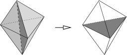
Figure 4: A 3-2 Pachner move

The condition of Lemma 2.1.1 requiring the degree three edge to belong to three distinct tetrahedra is indeed necessary. There do exist closed minimal $\mathbb{P}^{2}$-irreducible triangulations containing edges of degree three that belong to only two tetrahedra (by representing multiple edges of one of these tetrahedra). Examples of such triangulations are described in detail by Jaco and Rubinstein [7].

Disqualifying edges of degree one or two is more difficult than disqualifying edges of degree three. To assist in this task we present the following simple result.

Lemma 2.1.2

No closed minimal $\mathbb{P}^{2}$-irreducible triangulation with $\geq 3$ tetrahedra contains an embedded non-separating 2-sphere or an embedded projective plane.

Proof.

By $\mathbb{P}^{2}$-irreducibility, any embedded 2-sphere bounds a ball and is thus separating. Consider then an embedded projective plane $P$. By $\mathbb{P}^{2}$-irreducibility again we see that $P$ is one-sided, and so a regular neighbourhood of $P$ has 2-sphere boundary and is in fact $\mathbb{R}P^{3}$ with a ball removed.

Using $\mathbb{P}^{2}$-irreducibility once more it follows that this 2-sphere boundary must bound a ball on the side away from $P$ and so our entire triangulation is of the 3-manifold $\mathbb{R}P^{3}$. We observe that $\mathbb{R}P^{3}$ can be triangulated using two tetrahedra as seen in Appendix A and so our triangulation cannot be minimal. ∎

Lemma 2.1.3 (Degree Two Edges)

No closed minimal $\mathbb{P}^{2}$-irreducible triangulation with $\geq 3$ tetrahedra contains an edge of degree two.

Proof.

Let $e$ be an edge of degree two in a closed minimal $\mathbb{P}^{2}$-irreducible triangulation with $\geq 3$ tetrahedra. If $e$ belongs to only one tetrahedron then it must appear as two distinct edges of that tetrahedron. Figure 5 lists the three possible arrangements in which this is possible.

\psfrag{I}{{\small I}}\psfrag{II}{{\small II}}\psfrag{III}{{\small III}}\psfrag{e}{{\small$e$}}\includegraphics[scale={0.7}]{censusdegree2.eps}

Figure 5: An edge of degree two belonging to only one tetrahedron

In case I, edge $e$ lies in all four faces of the tetrahedron. However, since $e$ has degree two it can only belong to two faces of the overall triangulation. Thus these four faces are identified in pairs and the triangulation cannot have more than one tetrahedron.

In cases II and III, the bottom face of the tetrahedron contains edge $e$ twice and must therefore be identified with some other face of the tetrahedron also containing edge $e$ twice. There is however no other such face and so neither of these cases can occur.

\psfrag{e}{{\small$e$}}\psfrag{g}{{\small$g$}}\psfrag{h}{{\small$h$}}\psfrag{A}{{\small$A$}}\psfrag{B}{{\small$B$}}\psfrag{C}{{\small$C$}}\psfrag{D}{{\small$D$}}\includegraphics[scale={0.7}]{censusdegree2-2.eps}

Figure 6: An edge of degree two belonging to two tetrahedra

Thus $e$ must belong to two distinct tetrahedra as depicted in Figure 6. Consider edges $g$ and $h$ as marked in the diagram. If these edges are identified, the disc between them forms either a 2-sphere or a projective plane. If it forms a projective plane then this projective plane is embedded, contradicting Lemma 2.1.2.

If the disc between edges $g$ and $h$ forms a 2-sphere, we claim that this 2-sphere must be separating. If the 2-sphere does not intersect itself then it is separating by a direct application of Lemma 2.1.2. Otherwise the only way in which the 2-sphere can intersect itself is if the two vertices at the endpoints of $g$ and $h$ are identified. In this case we deform the 2-sphere slightly by pulling it away from these vertices within the 3-manifold, resulting in an embedded 2-sphere which from Lemma 2.1.2 is again separating.

So assuming this disc forms a separating 2-sphere, cutting along it splits the underlying 3-manifold into a connected sum decomposition. Since the triangulation is $\mathbb{P}^{2}$-irreducible, one side of this disc must bound a ball; without loss of generality let it be the side containing faces $A$ and $C$. The triangulation can then be simplified without changing the underlying 3-manifold by removing this ball and flattening the disc to a single edge, converting Figure 6 to a triangular pillow bounded by faces $B$ and $D$ as illustrated in Figure 7.

\psfrag{e}{{\small$e$}}\psfrag{g}{{\small$g$}}\psfrag{h}{{\small$h$}}\psfrag{gh}{{\small$g,h$}}\psfrag{A}{{\small$A$}}\psfrag{B}{{\small$B$}}\psfrag{C}{{\small$C$}}\psfrag{D}{{\small$D$}}\includegraphics[scale={0.7}]{censusdegree2-split.eps}

Figure 7: Simplifying the triangulation by removing a ball

If faces $B$ and $D$ are identified, the 3-manifold must be either the 3-sphere or $L(3,1)$ (the two spaces obtainable by identifying the faces of a triangular pillow). Our original triangulation is therefore non-minimal since each of these spaces can be realised with $\leq 2$ tetrahedra as seen in Appendix A. If faces $B$ and $D$ are not identified, the entire pillow can be flattened to a single face and our original triangulation has been reduced by two tetrahedra, once more showing it to be non-minimal.

The only case remaining is that in which edges $g$ and $h$ are not identified. In this case we may flatten the disc between edges $g$ and $h$ to a single edge, converting Figure 6 to a pair of triangular pillows as illustrated in the central diagram of Figure 8.

\psfrag{e}{{\small$e$}}\psfrag{g}{{\small$g$}}\psfrag{h}{{\small$h$}}\psfrag{A}{{\small$A$}}\psfrag{B}{{\small$B$}}\psfrag{C}{{\small$C$}}\psfrag{D}{{\small$D$}}\includegraphics[scale={0.7}]{censusdegree2-pillows.eps}

Figure 8: Flattening the region about an edge of degree two

Each of these pillows may then be flattened to a face as illustrated in the right hand diagram of Figure 8. The underlying 3-manifold is only changed if we attempt to flatten a pillow whose top and bottom faces are identified, in which case our 3-manifold must again be $S^{3}$ or $L(3,1)$ and so our original triangulation is non-minimal. Otherwise we have reduced our triangulation by two tetrahedra, once more a contradiction to minimality. ∎

Lemma 2.1.4 (Degree One Edges)

No closed minimal $\mathbb{P}^{2}$-irreducible triangulation with $\geq 3$ tetrahedra contains an edge of degree one.

Proof.

The only way of creating an edge of degree one in a 3-manifold triangulation is to fold two faces of a tetrahedron together around the edge between them, as illustrated in Figure 9 where $e$ is the edge of degree one.

\psfrag{e}{{\small$e$}}\includegraphics[scale={0.7}]{censusedgedeg1.eps}

Figure 9: An edge of degree one

Since our triangulation has $\geq 3$ tetrahedra, the two remaining faces of this tetrahedron cannot be identified with each other. Let the upper face then be joined to some other tetrahedron as illustrated in the left hand diagram of Figure 10. Let $g$ and $h$ be the two edges of this new tetrahedron running from $A$ to $C$ as marked in the diagram.

\psfrag{A}{{\small$A$}}\psfrag{B}{{\small$B$}}\psfrag{C}{{\small$C$}}\psfrag{D}{{\small$D$}}\psfrag{e}{{\small$e$}}\psfrag{g}{{\small$g$}}\psfrag{h}{{\small$h$}}\psfrag{gh}{{\small$g,h$}}\psfrag{(M)}{{\small($M$)}}\psfrag{(N)}{{\small($N$)}}\includegraphics[scale={0.7}]{census21sum.eps}

Figure 10: Splitting apart a connected sum

If edges $g$ and $h$ are identified, the disc between them forms either a 2-sphere or a projective plane. Assuming our triangulation is minimal and $\mathbb{P}^{2}$-irreducible, the same argument used in the proof of Lemma 2.1.3 shows that this disc must be a separating 2-sphere.

In this case, cutting along the disc between edges $g$ and $h$ therefore splits our 3-manifold into two separate pieces each with 2-sphere boundary. Flattening this disc to a single edge effectively fills in each of these 2-sphere boundary components with balls, producing closed 3-manifolds $M$ and $N$ for which our original 3-manifold is the connected sum $M\#N$.

This procedure is illustrated in the right hand diagram of Figure 10, where $M$ includes the portion above edge $AC$ (including vertex $B$) and $N$ includes the portion below edge $AC$ (including vertex $D$). Note that the portion of the diagram between vertices $A$, $C$ and $B$ forms a triangular pillow, which can be retriangulated using two tetrahedra with a new internal vertex as illustrated. The portion between vertices $A$, $C$ and $D$ can be retriangulated using a single tetrahedron with a new internal edge of degree one, much like our original Figure 9.

Since our original 3-manifold is $\mathbb{P}^{2}$-irreducible but is also expressible as the connected sum $M\#N$, it follows that one of $M$ or $N$ is a 3-sphere and the other is a new triangulation of this original 3-manifold. If $M$ is the 3-sphere, we see that $N$ is a triangulation of the original 3-manifold formed from one fewer tetrahedron. If $N$ is the 3-sphere then $M$ is a new triangulation of our original 3-manifold with no change in the number of tetrahedra. This new triangulation however contains three edges of degree two within the triangular pillow, and so from Lemma 2.1.3 it cannot be formed from the smallest possible number of tetrahedra. Either way we see that our original triangulation cannot be minimal.

The only remaining case is that in which edges $g$ and $h$ are not identified at all. Here we may flatten the disc between $g$ and $h$ to an edge without altering the underlying 3-manifold, as illustrated in the central diagram of Figure 11. The region between vertices $A$, $C$ and $D$ may be retriangulated using a single tetrahedron as before.

\psfrag{A}{{\small$A$}}\psfrag{B}{{\small$B$}}\psfrag{C}{{\small$C$}}\psfrag{D}{{\small$D$}}\psfrag{e}{{\small$e$}}\psfrag{g}{{\small$g$}}\psfrag{h}{{\small$h$}}\includegraphics[scale={0.7}]{census21.eps}

Figure 11: Flattening a region close to an edge of degree one

In this case we once more observe that the region between vertices $A$, $C$ and $B$ becomes a triangular pillow. Furthermore, it is impossible to identify the two faces bounding this pillow under any rotation or reflection without identifying edges $g$ and $h$ as a result. Hence the two faces bounding this pillow are distinct and we may flatten the pillow to a face as illustrated in the right-hand diagram of Figure 11 with no effect upon the underlying 3-manifold. The result is a new triangulation of our original 3-manifold with one fewer tetrahedron, and so again our original triangulation is non-minimal. ∎

2.2 Face Subcomplexes

In this section we identify a variety of simple structures formed from faces within a closed triangulation whose presence indicates that the triangulation cannot be both minimal and $\mathbb{P}^{2}$-irreducible.

For orientable triangulations, slightly restricted versions of these results can be seen as a consequence of Jaco and Rubinstein’s theory of 0-efficiency [7]. Here we prove these results using more elementary means, with generalisations in the orientable case and extensions to the non-orientable case.

Lemma 2.2.1 ($L(3,1)$ Spines)

Let $T$ be a closed minimal $\mathbb{P}^{2}$-irreducible triangulation containing $\geq 3$ tetrahedra. Then no face of $T$ has all three of its edges identified with each other in the same direction around the face, as illustrated in Figure 12.

Figure 12: A face with three identified edges

In Jaco and Rubinstein’s categorisation of face types within a triangulation [7], faces of this type are referred to as $L(3,1)$ spines for reasons that become apparent in the proof below.

Proof.

Consider a regular neighbourhood of the face in question. This regular neighbourhood can be expressed as a triangular prism, where the original face slices through the centre of the prism and the half-rectangles surrounding this central face are identified in pairs. Such structures can be seen in Figure 13, which depicts the two possible neighbourhoods that can be formed in this way up to rotation and reflection. In each diagram the original face with the three identified edges is shaded.

\psfrag{A}{{\small$A$}}\psfrag{B}{{\small$B$}}\psfrag{C}{{\small$C$}}\psfrag{D}{{\small$D$}}\psfrag{E}{{\small$E$}}\psfrag{F}{{\small$F$}}\psfrag{X}{{\small$X$}}\psfrag{Y}{{\small$Y$}}\psfrag{Z}{{\small$Z$}}\includegraphics[scale={0.7}]{censusl31prism.eps}

Figure 13: Possible regular neighbourhoods of a face with three identified edges

In the left hand diagram the neighbourhood is orientable, with faces XYBA and ZXDF identified, faces YZCB and XYED identified and faces ZXAC and YZFE identified. It can be seen that the boundary of this prism is a 2-sphere and that the body of the prism forms the lens space $L(3,1)$ with a ball removed. Thus our original triangulation represents the connected sum $M\#L(3,1)$ for some $M$, whereby $\mathbb{P}^{2}$-irreducibility implies that it must represent $L(3,1)$ itself. Since $L(3,1)$ can be triangulated using only two tetrahedra (see Appendix A), it follows that triangulation $T$ cannot be minimal.

The neighbourhood illustrated in the right hand diagram of Figure 13 is non-orientable, with faces XYBA and ZXAC identified, faces YZCB and XYED identified and faces ZXDF and YZFE identified. Note that points $X$, $Y$ and $Z$ are all identified as a single vertex in the triangulation, marked by a black circle in the diagram. A closer examination shows the link of this vertex to be a Klein bottle, not a 2-sphere. Therefore in this case triangulation $T$ cannot represent a closed 3-manifold at all. ∎

Before proceeding further, we recount the following result regarding vertices within a minimal triangulation.

Lemma 2.2.2

Let $M$ be a closed $\mathbb{P}^{2}$-irreducible 3-manifold that is not $S^{3}$, $\mathbb{R}P^{3}$ or the lens space $L(3,1)$. Then every minimal triangulation of $M$ has precisely one vertex.

Proof.

This result is proven explicitly by Jaco and Rubinstein [7] for orientable 3-manifolds. In the general case, Martelli and Petronio [10] prove an equivalent result regarding special spines of 3-manifolds. ∎

The following results eliminate cones within a triangulation formed from a small number of faces. These can be seen as generalisations of the low degree edge results of Section 2.1.

Lemma 2.2.3 (Two-Face Cones)

Let $T$ be a closed $\mathbb{P}^{2}$-irreducible triangulation containing $\geq 3$ tetrahedra. Suppose that two distinct faces of $T$ are joined together along their edges to form a cone as illustrated in Figure 14. Note that it is irrelevant whether or not any of the four edges of this cone (two internal edges and two boundary edges) are identified with each other in the overall triangulation.

Figure 14: Two faces joined together to form a cone

Since the two faces of this cone are distinct, if the interior of the cone intersects itself then these self-intersections can only take place along the two interior edges. In addition then, suppose that any such self-intersections are tangential and not transverse, as illustrated in Figure 15. If all of these conditions are met then $T$ cannot be a minimal triangulation.

\psfrag{Tangential}{{\small Tangential}}\psfrag{Transverse}{{\small Transverse}}\includegraphics[scale={0.6}]{transverse.eps}

Figure 15: Tangential and transverse intersections

Proof.

A similar result is proven by Martelli and Petronio in the orientable case using special spines of 3-manifolds [9]. We mirror a key construction of their proof for use in the general case here.

Before beginning, we observe that if triangulation $T$ represents one of the 3-manifolds $S^{3}$, $\mathbb{R}P^{3}$ or $L(3,1)$ then $T$ cannot be minimal, since each of these 3-manifolds can be triangulated using one or two tetrahedra as seen in Appendix A. We assume then that $T$ is a triangulation of some other 3-manifold.

Let the two faces of the cone be $F$ and $G$ with interior vertex $v$, as illustrated in the left hand diagram of Figure 16. Note that this cone forms a disc which is by necessity two-sided, and furthermore recall that all self-intersections of the interior of the cone are tangential. We can therefore expand faces $F$ and $G$ into two new tetrahedra as illustrated in the right hand diagram of Figure 16. Vertex $v$ is pulled apart into two distinct vertices $v_{1}$ and $v_{2}$, joined by a new internal edge $e$ of degree two. Faces $F$ and $G$ are similarly pulled apart into four distinct faces $F_{1}$, $F_{2}$, $G_{1}$ and $G_{2}$.

\psfrag{v}{{\small$v$}}\psfrag{v1}{{\small$v_{1}$}}\psfrag{v2}{{\small$v_{2}$}}\psfrag{F}{{\small$F$}}\psfrag{F1}{{\small$F_{1}$}}\psfrag{F2}{{\small$F_{2}$}}\psfrag{G}{{\small$G$}}\psfrag{G1}{{\small$G_{1}$}}\psfrag{G2}{{\small$G_{2}$}}\psfrag{e}{{\small$e$}}\psfrag{g}{{\small$g$}}\psfrag{h}{{\small$h$}}\includegraphics[scale={0.6}]{twofaceconeexpand.eps}

Figure 16: Expanding a two-face cone into two tetrahedra

Call the resulting triangulation $T^{\prime}$. If the original triangulation $T$ is formed from $t$ tetrahedra then $T^{\prime}$ is formed from precisely $t+2$ tetrahedra. Furthermore, $T^{\prime}$ contains at least two vertices since $v_{1}$ and $v_{2}$ are distinct. At this point we attempt to simplify $T^{\prime}$ using a similar set of operations to those used in the proof of Lemma 2.1.3. These operations are illustrated in Figure 17.

\psfrag{v}{{\small$v$}}\psfrag{v1}{{\small$v_{1}$}}\psfrag{v2}{{\small$v_{2}$}}\psfrag{F}{{\small$F$}}\psfrag{F1}{{\small$F_{1}$}}\psfrag{F2}{{\small$F_{2}$}}\psfrag{G}{{\small$G$}}\psfrag{G1}{{\small$G_{1}$}}\psfrag{G2}{{\small$G_{2}$}}\psfrag{e}{{\small$e$}}\psfrag{d}{{\small$\delta$}}\psfrag{g}{{\small$g$}}\psfrag{h}{{\small$h$}}\includegraphics[scale={0.6}]{twofaceconesimp.eps}

Figure 17: Simplifying the expanded triangulation $T^{\prime}$

Let $g$ and $h$ be the edges circling $e$ as marked in the left hand diagram of Figure 17, and let $\delta$ be the disc that they bound. Our first step is to flatten $\delta$ to a single edge as illustrated in the central diagram of Figure 17. If $g$ and $h$ are distinct edges of $T^{\prime}$ then flattening $\delta$ has no effect upon the underlying 3-manifold. Alternatively, if $g$ and $h$ are identified in $T^{\prime}$ then we can use $\mathbb{P}^{2}$-irreducibility as in the proofs of Lemmas 2.1.3 and 2.1.4 to show that the disc $\delta$ must form a separating 2-sphere. In this case, flattening $\delta$ to an edge corresponds to slicing along this 2-sphere and filling the resulting boundary components with balls. That is, the underlying 3-manifold is broken up into a connected sum decomposition.

At this stage the two new tetrahedra have become two triangular pillows. Each of these pillows can then be flattened to a face as illustrated in the right hand diagram of Figure 17. Since all four faces $F_{1}$, $F_{2}$, $G_{1}$ and $G_{2}$ are distinct, this flattening of pillows has no effect upon the underlying 3-manifold.

The final triangulation then has $t$ tetrahedra but more importantly has at least two vertices. If the underlying 3-manifold was not changed, it follows from Lemma 2.2.2 that this final triangulation is not minimal and so neither is $T$.

If the underlying 3-manifold was changed however, it was broken into a connected sum decomposition. By $\mathbb{P}^{2}$-irreducibility it follows that one of the summands must be a 3-sphere and the other must be the original 3-manifold. In this case we simply throw away the 3-sphere and obtain a triangulation of the original 3-manifold formed from strictly fewer than $t$ tetrahedra, once more showing the original triangulation $T$ to be non-minimal. ∎

Lemma 2.2.4 (One-Face Cones)

Let $T$ be a closed minimal $\mathbb{P}^{2}$-irreducible triangulation containing $\geq 3$ tetrahedra. Then no single face of $T$ has two of its edges identified to form a cone as illustrated in Figure 18. Note that it is irrelevant whether or not the third edge of the face is identified with the other two.

\psfrag{V}{{\small$v$}}\includegraphics[scale={0.7}]{facecone.eps}

Figure 18: A face with two edges identified to form a cone

Proof.

Suppose that some face $F$ has two of its edges identified to form a cone, where $v$ is the vertex joining both edges as marked in Figure 18. Consider the link of vertex $v$ within the 3-manifold triangulation. This link must be a 2-sphere formed from triangles, which we denote by $S$. Furthermore, face $F$ corresponds to a loop within this vertex link as illustrated in the left hand diagram of Figure 19.

\psfrag{I}{{\small I}}\psfrag{II}{{\small II}}\psfrag{III}{{\small III}}\includegraphics[scale={0.7}]{conelink.eps}

Figure 19: The inside of a loop in a vertex link

Since $S$ is a 2-sphere, this loop bounds a disc in the vertex link. The inside of this disc must appear as one of the three configurations shown on the right hand side of Figure 19, where the structures of the shaded regions remain unknown. Configuration I contains one or more inner loops; we can thus apply this same argument to the inner loops and continue deeper inside the disc until we eventually arrive at either configuration II or III.

In configuration II we see that the link $S$ contains a vertex of degree one. This corresponds to an edge of degree one in the 3-manifold triangulation, which from Lemma 2.1.4 cannot occur.

In configuration III, the two inner edges of the vertex link correspond to two faces $G$ and $H$ of the 3-manifold triangulation whose edges are identified to form a cone, as illustrated in the left hand diagram of Figure 20. Furthermore, the triangle wrapping around these edges in the vertex link corresponds to a tetrahedron wrapping around faces $G$ and $H$ as seen in the right hand diagram of Figure 20.

\psfrag{G}{{\small$G$}}\psfrag{H}{{\small$H$}}\psfrag{v}{{\small$v$}}\includegraphics[scale={0.7}]{conebody.eps}

Figure 20: Faces corresponding to the two inner edges of the vertex link

If faces $G$ and $H$ are distinct, we call upon Lemma 2.2.3 to secure the result. The tetrahedron wrapped around these faces ensures that the required tangentiality condition is met, and so Lemma 2.2.3 can be applied to show that triangulation $T$ is non-minimal.

Figure 21: A face with two corners identified to form a cone

Otherwise $G$ and $H$ must in fact be the same face of the 3-manifold triangulation, where the two inner edges of the vertex link correspond to two different corners of the face. For two different corners to meet in this way, this face must have all three edges identified as illustrated in Figure 21. Lemma 2.2.1 however shows that such a face cannot occur. ∎

Our next results concern pairs of faces that, when sliced open, combine to form small spherical boundary components of the resulting triangulation.

Lemma 2.2.5 (Spherical Subcomplexes)

Let $T$ be a closed triangulation with $\geq 3$ tetrahedra. Consider two faces $F_{1}$ and $F_{2}$ of $T$ that are joined along at least one edge.

Slicing $T$ along $F_{1}$ and $F_{2}$ will produce a new (possibly disconnected) triangulation with four boundary faces; call this $T^{\prime}$. Note that $T^{\prime}$ might have vertices whose links are neither spheres nor discs, and so might not actually represent one or more 3-manifolds.

If $T^{\prime}$ contains multiple boundary components (as opposed to a single four-face boundary component) and if one of these boundary components is a sphere as illustrated in Figure 22, then $T$ cannot be both minimal and $\mathbb{P}^{2}$-irreducible.

Figure 22: A sphere formed by identifying the boundaries of two triangles

Note that it does not matter if some vertices of this boundary sphere are identified, i.e., if the sphere is pinched at two or more points – this is indeed expected if $T^{\prime}$ has non-standard vertex links as suggested above. Only the edge identifications illustrated in Figure 22 are required for the conditions of this lemma to be met.

Proof.

Let $T$ be a minimal $\mathbb{P}^{2}$-irreducible triangulation satisfying all of the given conditions and consider the triangulation $T^{\prime}$ as described in the lemma statement. Recall that any boundary component must contain an even number of faces. Since $T^{\prime}$ has four boundary faces and multiple boundary components, it must therefore have precisely two boundary components each with two faces. Furthermore, since faces $F_{1}$ and $F_{2}$ are adjacent in $T$, each of these boundary components must be formed from a copy of both faces $F_{1}$ and $F_{2}$.

Let these two boundary components be $\partial_{1}$ and $\partial_{2}$ where $\partial_{1}$ is a sphere as illustrated in Figure 22. Let $R_{1}$ and $R_{2}$ represent the regions of $T^{\prime}$ just inside boundary components $\partial_{1}$ and $\partial_{2}$ respectively. Finally let $S$ be an embedded sphere located in $R_{1}$ just behind the spherical boundary component $\partial_{1}$. This scenario is illustrated in Figure 23.

\psfrag{R1}{{\small$R_{1}$}}\psfrag{R2}{{\small$R_{2}$}}\psfrag{d1}{{\small$\partial_{1}$}}\psfrag{d2}{{\small$\partial_{2}$}}\psfrag{S}{{\small$S$}}\includegraphics[scale={0.7}]{censustripillowsetup.eps}

Figure 23: Regions within the split triangulation $T^{\prime}$

As noted in the lemma statement, vertices of the boundary sphere $\partial_{1}$ might be identified and thus it may in fact be impossible to place the sphere $S$ entirely within region $R_{1}$. If this is the case then we simply push $S$ outside region $R_{1}$ in a small neighbourhood of each offending vertex. Examples of the resulting sphere $S$ are illustrated for two different cases in Figure 24.

\psfrag{R1}{{\small$R_{1}$}}\psfrag{d1}{{\small$\partial_{1}$}}\psfrag{S}{{\small$S$}}\includegraphics[scale={0.7}]{censustripillowpushs.eps}

Figure 24: Pushing sphere $S$ outside region $R_{1}$ in the neighbourhood of a vertex

We can now view $S$ as an embedded 2-sphere in the original triangulation $T$. Note that whenever $S$ is pushed outside region $R_{1}$ as described above, it is simply pushed into a small neighbourhood of a vertex in region $R_{2}$. In particular, since the link of each vertex of $T$ is a 2-sphere, such operations do not introduce any self-intersections in $S$.

Since $T$ is $\mathbb{P}^{2}$-irreducible it follows that the embedded 2-sphere $S$ must bound a ball in $T$. We take cases according to whether this ball lies on the side of $S$ including region $R_{1}$ or region $R_{2}$.

• Suppose that $S$ bounds a ball on the side containing region $R_{2}$. In this case we can remove the component of $T^{\prime}$ containing region $R_{2}$ and replace it with a two-tetrahedron triangular pillow as illustrated in Figure 25. This pillow can then be joined to region $R_{1}$ along the spherical boundary $\partial_{1}$ resulting in a new triangulation $T^{\prime\prime}$ whose underlying 3-manifold is identical to that of $T$.

  

  Figure 25: A replacement two-tetrahedron triangular pillow

• Otherwise $S$ bounds a ball on the side containing region $R_{1}$. In this case we remove the component of $T^{\prime}$ containing region $R_{1}$ and again replace it with the two-tetrahedron triangular pillow illustrated in Figure 25. The pillow has a spherical boundary identical to the old boundary $\partial_{1}$ and so it can be successfully dropped in as a replacement component without changing the underlying 3-manifold. Once more we denote this new triangulation $T^{\prime\prime}$, where the underlying 3-manifold of $T^{\prime\prime}$ is identical to that of $T$.

  Note that even if the old component of $T^{\prime}$ containing region $R_{1}$ includes a vertex whose link is a multiply-punctured sphere, the underlying 3-manifolds of $T$ and $T^{\prime\prime}$ remain identical. Such a scenario is illustrated in the left hand diagram of Figure 26, with the replacement triangular pillow illustrated in the right hand diagram of the same figure. Since $S$ is pushed away from the vertex in question, it can be seen that in both triangulations $T$ and $T^{\prime\prime}$ the sphere $S$ bounds a ball on the side containing region $R_{1}$. Meanwhile the region on the other side of $S$ remains unchanged and so the underlying 3-manifold is preserved.

  \psfrag{R1}{{\small$R_{1}$}}\psfrag{d1}{{\small$\partial_{1}$}}\psfrag{S}{{\small$S$}}\psfrag{T/T'}{{\small$T$, $T^{\prime}$}}\psfrag{T''}{{\small$T^{\prime\prime}$}}\includegraphics[scale={0.7}]{censustripillowpunc.eps}

  Figure 26: A case involving a vertex whose link is a multiply-punctured sphere

We see then that in each of the above cases we have removed at least one tetrahedron and inserted two, resulting in a net increase of at most one tetrahedron. However, since the two original faces $F_{1}$ and $F_{2}$ were distinct, we can flatten the triangular pillow of Figure 25 to a single face in the new triangulation $T^{\prime\prime}$. The resulting triangulation has the same underlying 3-manifold as before but now uses at least one fewer tetrahedron than the original triangulation $T$. Thus triangulation $T$ cannot be minimal. ∎

Corollary 2.2.6

Let $T$ be a closed triangulation with $\geq 3$ tetrahedra. If $T$ contains two faces whose edges are identified to form a sphere as illustrated in Figure 22 and if the three edges of this sphere are distinct (i.e., none are identified with each other in the triangulation), then $T$ cannot be both minimal and $\mathbb{P}^{2}$-irreducible.

Proof.

Since the three edges of this sphere are distinct, the sphere has no self-intersections except possibly at the vertices of its two faces. Combined with the fact that all spheres within a 3-manifold are two-sided, we see that slicing $T$ along the two faces in question produces two spherical boundary components that are each triangulated as illustrated in Figure 22. Thus Lemma 2.2.5 can be invoked and $T$ cannot be both minimal and $\mathbb{P}^{2}$-irreducible. ∎

The final result of this section, though not strictly falling into the category of face subcomplexes, nevertheless helps lighten some of the case analyses that take place in Section 3.

Lemma 2.2.7

Let $T$ be a closed minimal $\mathbb{P}^{2}$-irreducible triangulation in which $e$ is an edge. Consider a ring of adjacent tetrahedra $\Delta_{1},\ldots,\Delta_{k}$ about edge $e$ as illustrated in the left hand diagram of Figure 27. Note that the same tetrahedron may appear multiple times in this list, since edge $e$ may correspond to multiple edges of the same tetrahedron. Let $F$ and $G$ be the two faces at either end of this ring, so that faces $F$ and $G$ belong to tetrahedra $\Delta_{1}$ and $\Delta_{k}$ respectively and are adjacent along edge $e$. These two faces are shaded in the diagram.

\psfrag{e}{{\small$e$}}\psfrag{d1}{{\small$\Delta_{1}$}}\psfrag{d2}{{\small$\Delta_{2}$}}\psfrag{dd}{{\small$\Delta_{k}$}}\psfrag{F}{{\small$F$}}\psfrag{G}{{\small$G$}}\psfrag{P}{{\small$P$}}\psfrag{Q}{{\small$Q$}}\psfrag{R}{{\small$R$}}\psfrag{S}{{\small$S$}}\includegraphics[scale={0.7}]{tetring.eps}

Figure 27: A ring of tetrahedra about edge $e$

If faces $F$ and $G$ are identified in triangulation $T$, then this identification must be orientation-preserving within the ring of tetrahedra. That is, either the two faces are folded together over edge $e$ or the two faces are folded together with a $120^{\circ}$ twist.

More specifically, if the vertices of faces $F$ and $G$ are labelled $P$, $Q$, $R$ and $S$ as indicated in the right hand diagram of Figure 27, then face PRS may be identified with either QRS, RSQ or SQR (where the order of vertices indicates the specific rotation or reflection used). None of the orientation-reversing identifications in which PRS is identified with QSR, SRQ or RQS may be used.

Proof.

If face PRS is identified with QSR then edge $e$ is identified with itself in reverse and so $T$ cannot be a 3-manifold triangulation. If face PRS is identified with SRQ then edges PR and SR of face $F$ are identified to form a cone, contradicting Lemma 2.2.4. Identifying faces PRS and RQS similarly produces a cone in contradiction to Lemma 2.2.4. ∎

3 Main Results

Equipped with the preliminary results of Section 2, we can begin to prove our main results involving face pairing graphs and minimal triangulations. These results can be split into two categories. In Section 3.1 we use face pairing graphs to derive structural properties of the corresponding triangulations. Section 3.2 on the other hand establishes properties of the face pairing graphs themselves.

3.1 Structural Properties of Triangulations

Recall from Definition 1.2.1 that each edge within a face pairing graph corresponds to a pair of tetrahedron faces that are identified in a triangulation. A triangulation cannot be entirely reconstructed from its face pairing graph however, since each pair of faces can be identified in one of six different ways (three possible rotations and three possible reflections).

In this section we identify certain subgraphs within face pairing graphs and deduce information about the specific rotations and reflections under which the corresponding tetrahedron faces are identified.

A key structure that appears frequently within minimal triangulations and is used throughout the following results is the layered solid torus. Layered solid tori have been discussed in a variety of informal contexts by Jaco and Rubinstein. They appear in [7] and are treated thoroughly by these authors in [8]. Analogous constructs involving special spines of 3-manifolds have been described in detail by Matveev [12] and by Martelli and Petronio [11].

In order to describe the construction of a layered solid torus we introduce the process of layering. Layering is a transformation that, when applied to a triangulation with boundary, does not change the underlying 3-manifold but does change the curves formed by the boundary edges of the triangulation.

Definition 3.1.1 (Layering)

Let $T$ be a triangulation with boundary and let $e$ be one of its boundary edges. To layer a tetrahedron on edge $e$, or just to layer on edge $e$, is to take a new tetrahedron $\Delta$, choose two of its faces and identify them with the two boundary faces on either side of $e$ without twists. This procedure is illustrated in Figure 28.

\psfrag{e}{{\small$e$}}\psfrag{f}{{\small$f$}}\psfrag{T}{{\small$\Delta$}}\psfrag{M}{{\small$T$}}\includegraphics[width=156.49014pt]{layering.eps}

Figure 28: Layering a tetrahedron on a boundary edge

Note that layering on a boundary edge does not change the underlying 3-manifold; the only effect is to thicken the boundary around edge $e$. Note furthermore that edge $e$ is no longer a boundary edge, and instead edge $f$ (which in general represents a different curve on the boundary of the 3-manifold) has been added as a new boundary edge.

Definition 3.1.2 (Layered Solid Torus)

A standard layered solid torus is a triangulation of a solid torus formed as follows. We begin with the Möbius band illustrated in Figure 29, where the two edges marked $e$ are identified according to the arrows and where edge $g$ is a boundary edge. If we thicken this Möbius band slightly, we can imagine it as a solid torus with two boundary faces, one on each side of the Möbius band.

\psfrag{e}{{\small$e$}}\psfrag{f}{{\small$f$}}\psfrag{g}{{\small$g$}}\includegraphics[scale={0.7}]{layermobius.eps}

Figure 29: A one-triangle Möbius band

We make an initial layering upon one of the boundary edges corresponding to edge $e$. This results in a one-tetrahedron triangulation of a solid torus as illustrated in Figure 30. The new tetrahedron in the illustration is sliced in half; this tetrahedron in fact sits on top of the Möbius band, runs off the diagram to the right and returns from the left to simultaneously sit beneath the Möbius band.

\psfrag{e}{{\small$e$}}\psfrag{g}{{\small$g$}}\includegraphics[scale={0.7}]{layermobiusstandard.eps}

Figure 30: A one-tetrahedron standard layered solid torus

We then perform some number of additional layerings upon boundary edges, one at a time. We may layer as many times we like or we may make no additional layerings at all. There are thus infinitely many different standard layered solid tori that can be constructed.

Note that a non-standard layered solid torus can be formed by making the initial layering upon edge $g$ of the Möbius band instead of edge $e$, and that the Möbius band itself can be considered a degenerate layered solid torus involving no layerings at all. Such structures however are not considered here.

We can observe that each layered solid torus has two boundary faces and represents the same underlying 3-manifold, i.e., the solid torus. What distinguishes the different layered solid tori is the different patterns of curves that their boundary edges make upon the boundary torus.

We return now to structures within face pairing graphs. In particular we take an interest in chains within face pairing graphs, as defined below.

Definitions 3.1.3 (Chain)

A chain of length $k$ is the multigraph formed as follows. Take $k+1$ vertices labelled $0,1,2,\ldots,k$ and join vertices $i$ and $i+1$ with a double edge for all $0\leq i\leq k-1$. Each of these edges is called an interior edge of the chain.

If a loop is added joining vertex 0 to itself the chain becomes a one-ended chain. If another loop is added joining vertex $k$ to itself the chain becomes a double-ended chain (and is now a 4-valent multigraph). These loops are called end edges of the chain.

Example 3.1.4

A one-ended chain of length 4 is illustrated in Figure 31, and a double-ended chain of length 3 is illustrated in Figure 32.

Figure 31: A one-ended chain in a face pairing graph

Figure 32: A double-ended chain in a face pairing graph

It can be observed that a one-ended chain of length $k$ is in fact the face pairing graph of a standard layered solid torus containing $k+1$ tetrahedra. Our first major result regarding face pairing graphs is a strengthening of this relationship as follows.

Theorem 3.1.5

Let $T$ be a closed minimal $\mathbb{P}^{2}$-irreducible triangulation with $\geq 3$ tetrahedra and face pairing graph $G$. If $G$ contains a one-ended chain then the tetrahedra of $T$ corresponding to the vertices of this one-ended chain form a standard layered solid torus in $T$.

Proof.

We prove this by induction on the chain length. A one-ended chain of length 0 consists of a single vertex with a single end edge, representing a single tetrahedron with two of its faces identified. Using Lemma 2.2.7 with a ring of just one tetrahedron we see that these faces must be identified in an orientation-preserving fashion.

If these faces are simply snapped shut as illustrated in the left hand diagram of Figure 33 (faces ABC and DBC being identified), the edge between them will have degree one in the final triangulation which cannot happen according to Lemma 2.1.4. Thus these faces are identified with a twist as illustrated in the right hand diagram of Figure 33 (faces ABC and BCD being identified), producing a one-tetrahedron standard layered solid torus.

\psfrag{A}{{\small$A$}}\psfrag{B}{{\small$B$}}\psfrag{C}{{\small$C$}}\psfrag{D}{{\small$D$}}\includegraphics[scale={0.6}]{onetetjoin.eps}

Figure 33: Different ways of identifying two faces of a single tetrahedron

Assume then that any one-ended chain of length $k$ must correspond to a standard layered solid torus (which will have $k+1$ tetrahedra), and consider a one-ended chain of length $k+1$. This one-ended chain is simply a one-ended chain of length $k$ with an extra double edge attached to the end, and so by our inductive hypothesis the corresponding $k+2$ tetrahedra must form a $(k+1)$-tetrahedron layered solid torus with an addition tetrahedron joined to its boundary along two faces.

By symmetry of the two-triangle torus which forms the layered solid torus boundary, we can picture the situation as shown in the left hand diagram of Figure 34. In this diagram face WXY of the new tetrahedron is to be joined directly to face ABC of the layered solid torus with no rotations or reflections, and face YZW of the new tetrahedron is to be joined to face CDA but possibly with the vertices identified in some different order, i.e., with the faces being rotated or reflected before they are identified. Applying Lemma 2.2.7 to the ring of tetrahedra about edge AC, we see that this identification of faces YZW and CDA must be orientation-preserving.

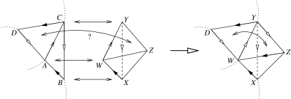
Figure 34: Attaching a new tetrahedron to a layered solid torus

If face YZW is simply folded over onto face CDA, i.e., the vertices are identified in this precise order with no rotation or reflection, then we have merely layered the new tetrahedron onto edge AC and so we obtain a larger standard layered solid torus with $k+2$ tetrahedra as required.

Otherwise a rotation must take place, and we may by symmetry assume that face YZW is identified with face ACD as illustrated in the right hand diagram of Figure 34. In this diagram we see that each of the two new boundary faces (XWZ and XYZ) has two edges identified to form a cone, in contradiction to Lemma 2.2.4. ∎

The following result corresponds to double edges in a face pairing graph, and is particularly helpful in easing the massive case analyses required for some of the theorems of Section 3.2.

Lemma 3.1.6

Let $T$ be a closed minimal $\mathbb{P}^{2}$-irreducible triangulation with $\geq 3$ tetrahedra. If two distinct tetrahedra of $T$ are joined to each other along two distinct faces then these two face identifications must be as illustrated in one of the diagrams of Figure 35.

\psfrag{A}{{\small$A$}}\psfrag{B}{{\small$B$}}\psfrag{C}{{\small$C$}}\psfrag{D}{{\small$D$}}\psfrag{a}{{\small$A^{\prime}$}}\psfrag{b}{{\small$B^{\prime}$}}\psfrag{c}{{\small$C^{\prime}$}}\psfrag{d}{{\small$D^{\prime}$}}\includegraphics[scale={0.7}]{censusdoubleedgegoodids.eps}

Figure 35: Allowable ways of joining two tetrahedra along two faces

Specifically, let the tetrahedra be ABCD and $A^{\prime}B^{\prime}C^{\prime}D^{\prime}$ with faces ABC and $A^{\prime}B^{\prime}C^{\prime}$ identified and with faces BCD and $B^{\prime}C^{\prime}D^{\prime}$ identified (though not necessarily with these precise vertex identifications; the faces may be rotated or reflected before they are identified). Then, allowing for the two tetrahedra to be relabelled and/or swapped, we must have one of the following three cases.

• Face ABC is identified with $A^{\prime}B^{\prime}C^{\prime}$ (no rotations or reflections take place) and face BCD is identified with $C^{\prime}D^{\prime}B^{\prime}$ (the faces are rotated before being identified); this is illustrated in the top left diagram of Figure 35.

• Face ABC is identified with $C^{\prime}A^{\prime}B^{\prime}$ and face BCD is identified with $C^{\prime}D^{\prime}B^{\prime}$ (both identifications involve a rotation in the same direction); this is illustrated in the top right diagram of Figure 35.

• Face ABC is identified with $C^{\prime}A^{\prime}B^{\prime}$ (the faces are rotated before being identified) and face BCD is identified with $B^{\prime}D^{\prime}C^{\prime}$ (the faces are reflected about a non-horizontal axis); this is illustrated in the bottom left diagram of Figure 35.

Note that the first two cases use consistent orientations for the two face identifications, whereas the third case results in a non-orientable structure.

Proof.

Consider initially the case in which face ABC is identified with face $A^{\prime}B^{\prime}C^{\prime}$ without reflection or rotation. Applying Lemma 2.2.7 to edge AB we see that the remaining face identification must be orientation-preserving. Thus either face BCD is rotated before being identified with $B^{\prime}C^{\prime}D^{\prime}$, resulting in the first case listed in the lemma statement, or face BCD is identified directly with $B^{\prime}C^{\prime}D^{\prime}$, resulting in edge BC having degree two in contradiction to Lemma 2.1.3.

Allowing for the tetrahedra to be relabelled and/or swapped, the only remaining methods of identifying the two pairs of faces are the second and third cases listed in the lemma statement plus the additional possibility illustrated in Figure 36.

\psfrag{A}{{\small$A$}}\psfrag{B}{{\small$B$}}\psfrag{C}{{\small$C$}}\psfrag{D}{{\small$D$}}\psfrag{a}{{\small$A^{\prime}$}}\psfrag{b}{{\small$B^{\prime}$}}\psfrag{c}{{\small$C^{\prime}$}}\psfrag{d}{{\small$D^{\prime}$}}\includegraphics[scale={0.7}]{doubleedgebad.eps}

Figure 36: An unallowable way of joining two tetrahedra along two faces

In this remaining possibility, face ABC is identified with $B^{\prime}C^{\prime}A^{\prime}$ and face BCD is identified with $C^{\prime}D^{\prime}B^{\prime}$, i.e., both identifications involve a rotation but in opposite directions. In this case, faces ABD and $A^{\prime}C^{\prime}D^{\prime}$ each have two edges identified to form a cone in contradiction to Lemma 2.2.4. ∎

3.2 Properties of Face Pairing Graphs

In contrast to Section 3.1 which analyses the structures of triangulations based upon their face pairing graphs, in this section we derive properties of the face pairing graphs themselves. More specifically, we identify various types of subgraph that can never occur within a face pairing graph of a closed minimal $\mathbb{P}^{2}$-irreducible triangulation.

Theorem 3.2.1

Let $G$ be a face pairing graph on $\geq 3$ vertices. If $G$ contains a triple edge (two vertices joined by three distinct edges as illustrated in Figure 37), then $G$ cannot be the face pairing graph of a closed minimal $\mathbb{P}^{2}$-irreducible triangulation.

Figure 37: A triple edge in a face pairing graph

Proof.

Suppose that $T$ is a closed minimal $\mathbb{P}^{2}$-irreducible triangulation with $\geq 3$ tetrahedra whose face pairing graph contains a triple edge. Observe that this triple edge corresponds to two distinct tetrahedra of $T$ that are joined along three different faces. We enumerate all possible ways in which this can be done and derive a contradiction in each case.

Let these two tetrahedra be ABCD and $A^{\prime}B^{\prime}C^{\prime}D^{\prime}$ as illustrated in Figure 38. Faces ABD and $A^{\prime}B^{\prime}D^{\prime}$ are identified, faces BCD and $B^{\prime}C^{\prime}D^{\prime}$ are identified and faces CAD and $C^{\prime}A^{\prime}D^{\prime}$ are identified, though not necessarily with these specific vertex identifications; faces may be rotated or reflected before they are identified.

\psfrag{A}{{\small$A$}}\psfrag{B}{{\small$B$}}\psfrag{C}{{\small$C$}}\psfrag{D}{{\small$D$}}\psfrag{a}{{\small$A^{\prime}$}}\psfrag{b}{{\small$B^{\prime}$}}\psfrag{c}{{\small$C^{\prime}$}}\psfrag{d}{{\small$D^{\prime}$}}\includegraphics[scale={0.7}]{censustripleedgetets.eps}

Figure 38: Two tetrahedra to be joined along three faces

Faces ABC and $A^{\prime}B^{\prime}C^{\prime}$ remain unaccounted for, though they cannot be identified with each other since this would produce a 2-tetrahedron triangulation. Thus faces ABC and $A^{\prime}B^{\prime}C^{\prime}$ are distinct faces of $T$; we refer to these as the boundary faces since they bound the subcomplex formed by the two tetrahedra under investigation.

Each specific method of joining our two tetrahedra along the three pairs of faces is denoted by a matching string. A matching string is a sequence of three symbols representing the transformations that are applied to faces ABD, BCD and CAD respectively before they are identified with their counterparts from the second tetrahedron. Each symbol is one of the following.

• $\iota$: No transformation is applied.

• $\kappa$: The face is rotated clockwise.

• $\alpha$: The face is rotated anticlockwise.

• $c$: The face is reflected so that the centre point of the diagram (i.e., point $D$) remains fixed.

• $l$: The face is reflected so that the point at the clockwise end of the face (e.g., point $B$ on face ABD) remains fixed.

• $r$: The face is reflected so that the point at the anticlockwise end of the face (e.g., point $A$ on face ABD) remains fixed.

A full list of precise face identifications corresponding to each symbol is given in Table 1.

$\begin{array}[]{|c|cccccc|}\hline\cr&\iota&\kappa&\alpha&c&l&r\\ \hline\cr ABD&A^{\prime}B^{\prime}D^{\prime}&B^{\prime}D^{\prime}A^{\prime}&D^{\prime}A^{\prime}B^{\prime}&B^{\prime}A^{\prime}D^{\prime}&D^{\prime}B^{\prime}A^{\prime}&A^{\prime}D^{\prime}B^{\prime}\\ BCD&B^{\prime}C^{\prime}D^{\prime}&C^{\prime}D^{\prime}B^{\prime}&D^{\prime}B^{\prime}C^{\prime}&C^{\prime}B^{\prime}D^{\prime}&D^{\prime}C^{\prime}B^{\prime}&B^{\prime}D^{\prime}C^{\prime}\\ CAD&C^{\prime}A^{\prime}D^{\prime}&A^{\prime}D^{\prime}C^{\prime}&D^{\prime}C^{\prime}A^{\prime}&A^{\prime}C^{\prime}D^{\prime}&D^{\prime}A^{\prime}C^{\prime}&C^{\prime}D^{\prime}A^{\prime}\\ \hline\cr\end{array}$

Table 1: Precise face identifications corresponding to each transformation symbol

We can then enumerate the matching strings for all possible ways of joining our two tetrahedra along these three pairs of faces. Each matching string is considered only once up to equivalence, where equivalence includes rotating the two tetrahedra, reflecting the two tetrahedra and swapping the two tetrahedra.

As an example, a list of all matching strings up to equivalence for which the three face identifications have consistent orientations (i.e., which do not contain both a symbol from $\{\iota,\kappa,\alpha\}$ and a symbol from $\{c,l,r\}$) is as follows.

$$\iota\iota\iota,~{}\iota\iota\kappa,~{}\iota\kappa\kappa,~{}\iota\kappa\alpha,~{}\kappa\kappa\kappa,~{}\kappa\kappa\alpha,~{}ccc,~{}ccl,~{}cll,~{}clr,~{}crl,~{}lll,~{}llr.$$

Note that matching strings $\iota\kappa\alpha$ and $\iota\alpha\kappa$ are equivalent by swapping the two tetrahedra, but that $clr$ and $crl$ are not.

A full list of all matching strings up to equivalence, allowing for both orientation-preserving and orientation-reversing face identifications, is too large to analyse by hand. We can however use Lemma 3.1.6 to restrict this list to a more manageable size.

Specifically, Lemma 3.1.6 imposes conditions upon how two tetrahedra may be joined along two faces. In a matching string, each pair of adjacent symbols represents a joining of the two tetrahedra along two faces. We can thus use this lemma to determine which symbols may be followed by which other symbols in a matching string. The results of this analysis are presented in Table 2.

Symbol	May be followed by	Cannot be followed by
$\iota$	$\kappa$, $\alpha$	$\iota$, $c$, $l$, $r$
$\kappa$	$\iota$, $\kappa$, $c$, $r$	$\alpha$, $l$
$\alpha$	$\iota$, $\alpha$, $c$, $r$	$\kappa$, $l$
$c$	$\kappa$, $\alpha$, $l$, $r$	$\iota$, $c$
$l$	$\kappa$, $\alpha$, $c$, $l$	$\iota$, $r$
$r$	$c$, $r$	$\iota$, $\kappa$, $\alpha$, $l$

Table 2: Possible adjacent symbols within a matching string

Up to rotation of the two tetrahedra, this reduces our list of possible matching strings to the following.

$$\iota\kappa\kappa,~{}\iota\alpha\alpha,~{}\kappa\kappa\kappa,~{}\alpha\alpha\alpha,~{}\kappa\kappa c,~{}\alpha\alpha c,~{}\kappa cl,~{}\kappa rc,~{}\alpha cl,~{}\alpha rc,~{}cll,~{}crr,~{}lll,~{}rrr.$$

Allowing for the two tetrahedra to be reflected and/or swapped, this list can be further reduced to just the following six matching strings.

$$\iota\kappa\kappa,~{}\kappa\kappa\kappa,~{}\kappa\kappa c,~{}\kappa cl,~{}cll,~{}lll.$$

These six matching strings can be split into three categories, where the matchings in each category give rise to a similar contradiction using almost identical arguments. We examine each category in turn.

• Conical faces ($\iota\kappa\kappa$, $\kappa cl$): Simply by following the edge identifications induced by our chosen face identifications, we can see that each of these matchings gives rise to a face containing two edges that are identified to form a cone. Lemma 2.2.4 then provides us with our contradiction.

  An example of this is illustrated in Figure 39 which shows the induced edge identifications for the matching $\kappa cl$. Conical faces in this example include ABD and the boundary face ABC.

  \psfrag{A}{{\small$A$}}\psfrag{B}{{\small$B$}}\psfrag{C}{{\small$C$}}\psfrag{D}{{\small$D$}}\psfrag{a}{{\small$A^{\prime}$}}\psfrag{b}{{\small$B^{\prime}$}}\psfrag{c}{{\small$C^{\prime}$}}\psfrag{d}{{\small$D^{\prime}$}}\includegraphics[scale={0.7}]{censustripleedgekcl.eps}

  Figure 39: Edge identifications for the matching $\kappa cl$

• Spherical subcomplexes ($\kappa\kappa\kappa$, $\kappa\kappa c$): Again we follow the induced edge identifications, but in this case the consequence is that the two boundary faces ABC and $A^{\prime}B^{\prime}C^{\prime}$ are joined at their edges to form a two-triangle sphere in contradiction to Lemma 2.2.5. This behaviour is illustrated in Figure 40 for the matching $\kappa\kappa c$.

  \psfrag{A}{{\small$A$}}\psfrag{B}{{\small$B$}}\psfrag{C}{{\small$C$}}\psfrag{D}{{\small$D$}}\psfrag{a}{{\small$A^{\prime}$}}\psfrag{b}{{\small$B^{\prime}$}}\psfrag{c}{{\small$C^{\prime}$}}\psfrag{d}{{\small$D^{\prime}$}}\includegraphics[scale={0.7}]{censustripleedgekkc.eps}

  Figure 40: Edge identifications for the matching $\kappa\kappa c$

• Bad vertex links ($cll$, $lll$): For these matching strings, all eight vertices $A$, $B$, $C$, $D$, $A^{\prime}$, $B^{\prime}$, $C^{\prime}$ and $D^{\prime}$ are identified as a single vertex in the triangulation. This vertex lies on the boundary faces ABC and $A^{\prime}B^{\prime}C^{\prime}$, and so the vertex link as restricted to our two tetrahedra will be incomplete (i.e., will have boundary components). However, for each of these matchings, this partial vertex link is observed to be a once-punctured torus. Therefore, however the entire triangulation $T$ is formed, the complete vertex link in $T$ cannot be a sphere (since there is no way to fill in the boundary of a punctured torus to form a sphere). Thus again we have a contradiction since $T$ cannot be a triangulation of a closed 3-manifold.

  As an example of this behaviour, Figure 41 illustrates the induced edge and vertex identifications for matching $lll$ as well as the corresponding vertex link. The link is shown as eight individual triangles followed by a combined figure, which we see is indeed a punctured torus.

  \psfrag{A}{{\small$A$}}\psfrag{B}{{\small$B$}}\psfrag{C}{{\small$C$}}\psfrag{D}{{\small$D$}}\psfrag{a}{{\small$A^{\prime}$}}\psfrag{b}{{\small$B^{\prime}$}}\psfrag{c}{{\small$C^{\prime}$}}\psfrag{d}{{\small$D^{\prime}$}}\includegraphics[scale={0.7}]{censustripleedgelll.eps}

  Figure 41: The partial vertex link for the matching $lll$

Thus we see that every method of identifying three faces of the first tetrahedron with three faces of the second gives rise to a contradiction, and so our result is established. ∎

Theorem 3.2.2

Let $G$ be a face pairing graph on $\geq 3$ vertices. If $G$ contains as a subgraph a broken double-ended chain (a double-ended chain missing one interior edge as illustrated in Figure 42) and if $G$ is not simply a double-ended chain itself, then $G$ cannot be the face pairing graph of a closed minimal $\mathbb{P}^{2}$-irreducible triangulation.

Figure 42: A broken double-ended chain in a face pairing graph

Proof.

Observe that a broken double-ended chain is merely a pair of one-ended chains joined by an edge. Let $T$ be a closed minimal $\mathbb{P}^{2}$-irreducible triangulation whose face pairing graph contains a broken double-ended chain. Then Theorem 3.1.5 implies that $T$ contains a pair of layered solid tori whose boundaries are joined along one face.

This situation is depicted in the left hand diagram of Figure 43, where the two torus boundaries of the layered solid tori are shown and where face ABC is identified with face XYZ. The resulting edge identifications of the remaining two boundary faces are illustrated in the right hand diagram of this figure; in particular, it can be seen that these remaining boundary faces form a two-triangle sphere (though with all three vertices pinched together, since each layered solid torus has only one vertex).

\psfrag{A}{{\small$A$}}\psfrag{B}{{\small$B$}}\psfrag{C}{{\small$C$}}\psfrag{X}{{\small$X$}}\psfrag{Y}{{\small$Y$}}\psfrag{Z}{{\small$Z$}}\psfrag{F1}{{\small$F_{1}$}}\psfrag{F2}{{\small$F_{2}$}}\includegraphics[scale={0.7}]{censuslstlstjoin.eps}

Figure 43: Two layered solid tori joined along a face

Let these remaining boundary faces be $F_{1}$ and $F_{2}$. If these faces are not identified then $F_{1}$ and $F_{2}$ satisfy the conditions of Lemma 2.2.5 and so $T$ cannot be both minimal and $\mathbb{P}^{2}$-irreducible. Therefore faces $F_{1}$ and $F_{2}$ are identified. Returning to the face pairing graph for $T$, this implies that the single edge between the two one-ended chains is in fact a double edge and so the graph contains an entire double-ended chain.

However, since every vertex in a double-ended chain has degree 4, Lemma 1.2.3 shows this double-ended chain to be the entire face pairing graph, contradicting the initial conditions of this theorem. ∎

Theorem 3.2.3

Let $G$ be a face pairing graph on $\geq 3$ vertices. If $G$ contains as a subgraph a one-ended chain with a double handle (a double-ended chain with one end edge replaced by a triangle containing one double edge as illustrated in Figure 44), then $G$ cannot be the face pairing graph of a closed minimal $\mathbb{P}^{2}$-irreducible triangulation.

Figure 44: A one-ended chain with a double handle in a face pairing graph

Proof.

Let $T$ be a closed minimal $\mathbb{P}^{2}$-irreducible triangulation with $\geq 3$ tetrahedra whose face pairing graph contains a one-ended chain with a double handle. From Theorem 3.1.5 we see that the one-ended chain must correspond to a layered solid torus in $T$. The double handle in turn must correspond to two additional tetrahedra each of which is joined to the other along two faces and each of which is joined to one of the boundary faces of the layered solid torus.

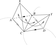
Figure 45: Tetrahedra corresponding to a one-ended chain with a double handle

This construction is illustrated in Figure 45. The layered solid torus lies beneath faces ABC and BCD which form its torus boundary. The two additional tetrahedra are XABC and YBCD; observe that each of these tetrahedra is joined to one of the boundary faces of the layered solid torus. The two new tetrahedra are then joined to each other along two faces; in this example faces XAC and YCB are identified and faces XCB and DCY are identified, though different pairs of faces may be used.

As in the proof of Theorem 3.2.1, we enumerate all possible ways in which this construction can be carried out and in each case derive a contradiction. To assist in our task we describe a simple way of representing each possible variant of this construction.

The scenario presented in Figure 45 can be distilled into a simplified diagram as illustrated in Figure 46. We begin with the two-triangle torus that forms the boundary of the layered solid torus as shown in the left hand diagram of Figure 46. We then add our two new tetrahedra, converting the two-triangle torus into a six-triangle torus as illustrated in the central diagram of Figure 46. Finally we add markings to the diagram to illustrate how the two new tetrahedra are to be joined along two faces. This is done by marking vertices $a$, $b$ and $c$ of the first face and vertices $x$, $y$ and $z$ of the second face. It can be seen from the right hand diagram of Figure 46 that faces XAC and YCB are identified and faces XCB and DCY are identified as described earlier. For clarity the two faces that have not yet been identified with any others are shaded.

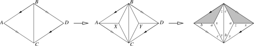
Figure 46: A simplified diagram for a one-ended chain with a double handle

In a similar fashion we can represent any set of tetrahedra corresponding to a one-ended chain with a double handle using a diagram similar to the right hand diagram of Figure 46. In this way we can enumerate all possible diagrams and in each case prove that $T$ cannot be a closed minimal $\mathbb{P}^{2}$-irreducible triangulation.

Recall from Lemma 3.1.6 that if $T$ is a closed minimal $\mathbb{P}^{2}$-irreducible triangulation then there are restrictions upon the possible ways in which our two new tetrahedra can be joined along two faces. Furthermore, Lemma 2.2.7 requires that if two adjacent faces are to be identified then this must be done in an orientation-preserving manner. By ignoring all diagrams that do not conform to Lemmas 2.2.7 and 3.1.6 and by exploiting the symmetries of the six-triangle torus and the layered solid torus that lies beneath it, we can reduce the set of all possible diagrams to those depicted in Figures 47 and 48. Figure 47 contains the diagrams for constructions that are orientation-preserving and Figure 48 contains the diagrams corresponding to non-orientable structures.

\psfrag{A1}{$\alpha_{1}$}\psfrag{A2}{$\alpha_{2}$}\psfrag{A3}{$\alpha_{3}$}\psfrag{B1}{$\beta_{1}$}\psfrag{B2}{$\beta_{2}$}\psfrag{B3}{$\beta_{3}$}\psfrag{C1}{$\gamma_{1}$}\psfrag{C2}{$\gamma_{2}$}\psfrag{C3}{$\gamma_{3}$}\psfrag{D1}{$\delta_{1}$}\psfrag{D2}{$\delta_{2}$}\includegraphics[scale={0.5}]{censusdoublehandlecasesor.eps}

Figure 47: All orientable diagrams for a one-ended chain with a double handle

\psfrag{A4}{$\alpha_{4}$}\psfrag{A5}{$\alpha_{5}$}\psfrag{A6}{$\alpha_{6}$}\psfrag{A7}{$\alpha_{7}$}\psfrag{B4}{$\beta_{4}$}\psfrag{B5}{$\beta_{5}$}\psfrag{D3}{$\delta_{3}$}\psfrag{D4}{$\delta_{4}$}\includegraphics[scale={0.5}]{censusdoublehandlecasesnor.eps}

Figure 48: All non-orientable diagrams for a one-ended chain with a double handle

As in the proof of Theorem 3.2.1 we can divide our 19 different diagrams $\alpha_{1},\ldots,\delta_{4}$ into a small number of categories, where the diagrams in each category give rise to similar contradictions using almost identical arguments. To assist with this process the edge identifications induced in each diagram by the corresponding face identifications are shown in Figures 49 and 50. The diagrams can then be split into categories as follows.

\psfrag{A1}{$\alpha_{1}$}\psfrag{A2}{$\alpha_{2}$}\psfrag{A3}{$\alpha_{3}$}\psfrag{B1}{$\beta_{1}$}\psfrag{B2}{$\beta_{2}$}\psfrag{B3}{$\beta_{3}$}\psfrag{C1}{$\gamma_{1}$}\psfrag{C2}{$\gamma_{2}$}\psfrag{C3}{$\gamma_{3}$}\psfrag{D1}{$\delta_{1}$}\psfrag{D2}{$\delta_{2}$}\includegraphics[scale={0.5}]{censusdoublehandlearrowsor.eps}

Figure 49: Edge identifications for the orientable face identification diagrams

\psfrag{A4}{$\alpha_{4}$}\psfrag{A5}{$\alpha_{5}$}\psfrag{A6}{$\alpha_{6}$}\psfrag{A7}{$\alpha_{7}$}\psfrag{B4}{$\beta_{4}$}\psfrag{B5}{$\beta_{5}$}\psfrag{D3}{$\delta_{3}$}\psfrag{D4}{$\delta_{4}$}\includegraphics[scale={0.5}]{censusdoublehandlearrowsnor.eps}

Figure 50: Edge identifications for the non-orientable face identification diagrams

• Conical faces ($\alpha_{1}$, $\alpha_{2}$, $\alpha_{4}$, $\alpha_{6}$, $\beta_{1}$, $\beta_{3}$, $\beta_{4}$, $\delta_{3}$, $\delta_{4}$): In each of these diagrams we find at least one face with two edges identified to form a cone. From Lemma 2.2.4 it follows that $T$ cannot be a closed minimal $\mathbb{P}^{2}$-irreducible triangulation.

• Spherical subcomplexes ($\alpha_{3}$, $\beta_{2}$, $\beta_{5}$, $\delta_{1}$): In each of these diagrams we can observe that the two shaded faces are joined at their edges to form a two-triangle sphere as described in Lemma 2.2.5, again contradicting the claim that $T$ is a closed minimal $\mathbb{P}^{2}$-irreducible triangulation.

• Bad vertex links ($\alpha_{5}$, $\alpha_{7}$, $\gamma_{1}$, $\gamma_{2}$, $\gamma_{3}$, $\delta_{2}$): In each of these diagrams it can be observed that all six vertices illustrated are in fact identified as a single vertex in the triangulation. We can calculate the link of this vertex as restricted to the portion of the triangulation that we are examining. For diagrams $\gamma_{1}$, $\gamma_{2}$ and $\gamma_{3}$ this link is observed to be a once-punctured torus, for diagram $\delta_{2}$ it is observed to be a once-punctured genus two torus and for diagrams $\alpha_{5}$ and $\alpha_{7}$ it is observed to be non-orientable. In each of these cases, however the remainder of the triangulation is constructed it is impossible for this vertex link to be extended to become a sphere. Thus $T$ cannot be a triangulation of a closed 3-manifold.

  The vertex link calculation is illustrated in Figure 51 for diagram $\gamma_{1}$. The disc on the left with edges $p$, $q$, $r$ and $s$ represents the vertex link of the layered solid torus and the triangles beside it represent the pieces of vertex link taken from the two new tetrahedra. These pieces are combined into a single surface on the right hand side of the diagram which we see is indeed a once-punctured torus.

  

  Figure 51: Calculating the vertex link for diagram $\gamma_{1}$

Thus for each diagram of Figure 47 and Figure 48 we observe that $T$ cannot be a closed minimal $\mathbb{P}^{2}$-irreducible triangulation. ∎

4 Enumeration of 3-Manifold Triangulations

We move now to the task of applying the results of Section 3 to the enumeration of closed minimal $\mathbb{P}^{2}$-irreducible triangulations. As described in the introduction, the enumeration of 3-manifold triangulations is a slow procedure typically based upon a brute force search through possible identifications of tetrahedron faces. Our aim then is to use the face pairing graph results of Section 3 to impose restrictions upon this brute force search and thus improve the performance of the algorithm.

Table 3 illustrates the performance of the enumeration algorithm before these new improvements are introduced. Included in the table are the counts up to isomorphism of closed minimal $\mathbb{P}^{2}$-irreducible triangulations formed from various numbers of tetrahedra, as well as the time taken by the computer to enumerate these triangulations. All times are displayed as h:mm:ss and are measured on a single 1.2GHz Pentium III processor. A time of 0:00 simply indicates a running time of less than half a second.

	Orientable		Non-Orientable
Tetrahedra	Triang.	Running Time	Triang.	Running Time
3	7	0:00	0	0:02
4	15	0:03	0	3:03
5	40	2:28	0	6:01:53
6	115	2:49:29	24	5 weeks

Table 3: Enumeration statistics without face pairing graph improvements

The enumerations described in Table 3 were performed by Regina [2], a freely available computer program that can perform a variety of calculations and procedures in 3-manifold topology. Statistics are not offered for one or two tetrahedra since these running times all round to 0:00.

In Section 4.1 we outline the structure of a typical enumeration algorithm and use the graph constraints derived in Section 3.2 to make some immediate efficiency improvements. Section 4.2 then uses the triangulation constraints derived in Section 3.1 to redesign the enumeration algorithm for a more significant increase in performance. Finally in Section 4.3 we present additional statistics to illustrate how well the newly designed algorithm performs in practice.

4.1 Eliminating Face Pairings

The algorithm for enumerating 3-manifold triangulations can be split into two largely independent tasks, these being the generation of face pairing graphs and the selection of rotations and reflections for the corresponding face identifications. This is a fairly natural way of approaching an enumeration of triangulations and is seen back in the earliest hyperbolic census of Hildebrand and Weeks [5]. Indeed this splitting of tasks appears to be used by all enumeration algorithms described in the literature, although different authors employ different variants of the general technique.

More specifically, a blueprint for an enumeration algorithm can be described as follows.

Algorithm 4.1.1 (Enumeration of Triangulations)

To enumerate up to isomorphism all 3-manifold triangulations formed from $n$ tetrahedra that satisfy some particular census constraints (such as minimality and $\mathbb{P}^{2}$-irreducibility), we perform the following steps.

1. Generate up to isomorphism all face pairings graphs for $n$ tetrahedra, i.e., all connected 4-valent multigraphs on $n$ vertices as described by Lemma 1.2.3.

2. For each generated face pairing graph, recursively try all possible rotations and reflections for each pair of faces to be identified.

   In general each pair of faces can be identified according to one of six possible rotations or reflections for non-orientable triangulations, or one of three possible rotations or reflections for orientable triangulations (allowing only the orientation-preserving identifications).

   Thus, with $2n$ pairs of identified faces, this requires a search through approximately $6^{2n}$ or $3^{2n}$ possible combinations of rotations and reflections for non-orientable or orientable triangulations respectively. In practice this search can be pruned somewhat. For instance, the results of Section 2.1 show that the search tree can be pruned where it becomes apparent that an edge of low degree will be present in the final triangulation. Other pruning techniques are described in the literature and frequently depend upon the specific census constraints under consideration.

3. For each triangulation thus constructed, test whether it satisfies the full set of census constraints and if so then include it in the final list of results.

In practise, the time spent generating face pairing graphs (step 1) is utterly negligible. For the six tetrahedron closed non-orientable census that consumed five weeks of processor time as seen in Table 3, the generation of face pairing graphs took under a hundredth of a second.

Our first improvement to Algorithm 4.1.1 is then as follows. When generating face pairing graphs in step 1 of Algorithm 4.1.1, we throw away any face pairing graphs that do not satisfy the properties proven in Section 3.2. Specifically we throw away face pairing graphs containing triple edges (Theorem 3.2.1), broken double-ended chains (Theorem 3.2.2) or one-ended chains with double handles (Theorem 3.2.3).

It is worth noting that Martelli and Petronio [9] employ a technique that likewise eliminates face pairing graphs for the purpose of enumerating bricks (a particular class of subcomplexes within 3-manifold triangulations). Their results are phrased in terms of special spines of 3-manifolds and relate to orientable triangulations satisfying specific structural constraints.

Since the enumeration of face pairing graphs is so fast, it seems plausible that if we can eliminate $p\%$ of all face pairing graphs in this way then we can eliminate approximately $p\%$ of the total running time of the algorithm. Table 4 illustrates how effective this technique is in practice. Specifically, it lists how many face pairing graphs on $n$ vertices for $3\leq n\leq 11$ contain each of the unallowable structures listed above. All counts are given up to isomorphism and were obtained using the program Regina [2].

The individual columns of Table 4 have the following meanings.

• Vertices: The number of vertices $n$.

• Total: The total number $t$ of connected 4-valent multigraphs on $n$ vertices.

• None: The number and percentage of graphs from this total $t$ in which none of the undesirable structures listed above were found.

• Some: The number of graphs from this total $t$ in which at least one of these undesirable structures was found.

• Triple: The number of graphs from the total $t$ that contain a triple edge.

• Broken: The number of graphs from the total $t$ that contain a broken double-ended chain.

• Handle: The number of graphs from the total $t$ that contain a one-ended chain with a double handle.

• Time: The running time taken to calculate the values in this row of the table. Running times are measured on a single 1.2GHz Pentium III processor and are displayed as h:mm:ss.

Note that the Total column should equal the None column plus the Some column in each row. Note also that the sum of the Triple, Broken and Handle columns might exceed the Some column since some graphs may contain more than one type of undesirable structure.

Vertices	Total	None		Some	Triple	Broken	Handle	Time
3	4	2	(50%)	2	1	1	1	0:00
4	10	4	(40%)	6	3	3	2	0:00
5	28	12	(43%)	16	8	10	4	0:00
6	97	39	(40%)	58	29	36	12	0:00
7	359	138	(38%)	221	109	137	40	0:01
8	1 635	638	(39%)	997	497	608	155	0:05
9	8 296	3 366	(41%)	4 930	2 479	2 976	685	0:44
10	48 432	20 751	(43%)	27 681	14 101	16 568	3 396	7:21
11	316 520	143 829	(45%)	172 691	88 662	102 498	18 974	1:20:48

Table 4: Frequency of undesirable structures within face pairing graphs

Examining Table 4 we see then that for each number of vertices a little over half of the possible face pairing graphs can be eliminated using the results of Section 3.2. Whilst this does not reduce the time complexity of the algorithm, it does allow us to reduce the running time by more than 50%, a significant improvement for a census that may take months or years to complete.

It is worth examining how comprehensive the theorems of Section 3.2 are. We turn our attention here specifically to the orientable case. Figure 52 lists all possible 3-vertex face pairing graphs, i.e., all connected 4-valent graphs on three vertices. A list of all possible 4-vertex face pairing graphs is provided in Figure 53. In each figure, the graphs to the left of the dotted line all lead to closed orientable minimal $\mathbb{P}^{2}$-irreducible triangulations whereas the graphs to the right of the dotted line do not. It can be seen that in both figures, every right hand graph contains either a triple edge, a broken double-ended chain or a one-ended chain with a double handle.

Figure 52: All possible face pairing graphs on three vertices

Figure 53: All possible face pairing graphs on four vertices

Thus for three and four tetrahedra, the results of Section 3.2 in fact perfectly divide the face pairings into those that lead to desirable triangulations and those that do not.

For five tetrahedra these theorems no longer perfectly divide the face pairings as we would like. Figure 54 lists all 5-vertex face pairing graphs; there are 28 in total. The 8 graphs in the top section all lead to closed orientable minimal $\mathbb{P}^{2}$-irreducible triangulations and the remaining 20 do not. Of these remaining 20, the 16 graphs in the middle section each contain a triple edge, a broken double-ended chain or a one-ended chain with a double handle. We see then that the final 4 graphs in the bottom section can never lead to a desirable triangulation but are not identified as such by the theorems of Section 3.2. Thus there remains more work to be done in the analysis of face pairing graphs.

Figure 54: All possible face pairing graphs on five vertices

4.2 Improved Generation of Rotations and Reflections

Consider once more Algorithm 4.1.1. This describes the enumeration algorithm as a three-stage process in which we generate face pairing graphs, generate rotations and reflections for each face pairing graph and then analyse the resulting triangulations. Recall from Section 4.1 that the running time spent generating face pairing graphs is inconsequential in the context of the overall enumeration algorithm. In fact almost the entire running time of the algorithm is spent in the second stage generating rotations and reflections.

As seen in step 2 of Algorithm 4.1.1 this generation of rotations and reflections is a recursive process in which we choose from six possibilities (or three for an orientable triangulation) for each pair of faces that are to be identified. This allows for up to $6^{2n}$ (or $3^{2n}$ for an orientable triangulation) different combinations of rotations and reflections for any given face pairing graph.

It is thus in the generation of rotations and reflections that we should seek to make the strongest improvements to the enumeration algorithm. Algorithm 4.1.1 already suggests techniques through which this recursion can be pruned and thus made faster. It is possible however that instead of chipping away at the recursion with more and more intricate pruning techniques, we could perhaps make more significant improvements by substantially redesigning the recursion using the face pairing graph results of Section 3.1.

Recall from Theorem 3.1.5 that every one-ended chain in a face pairing graph must correspond to a layered solid torus in the resulting triangulation. Recall also from Lemma 3.1.6 that every double edge in a face pairing graph must correspond to one of a restricted set of identifications of two tetrahedra along two faces. Instead of simply selecting rotations and reflections for each pair of faces one after another and pruning where possible, we can thus redesign the generation of rotations and reflections as follows.

1. Identify all one-ended chains in the face pairing graph. Recursively select a standard layered solid torus of the appropriate size to correspond to each of these one-ended chains.

2. Identify all remaining double edges in the face pairing graph, i.e., all double edges not belonging to the one-ended chains previously processed. For each such double edge recursively select an identification of the two corresponding tetrahedra conforming to Lemma 3.1.6.

3. At this point many of the individual rotations and reflections have already been established. Recursively select the remaining rotations and reflections as in the original algorithm, pruning where possible.

The first step of this redesigned algorithm should offer a substantial improvement in running time, as can be seen by the following rough calculations. In a one-ended chain on $k$ vertices there are $2k-1$ edges corresponding to $2k-1$ rotations and reflections that must be selected. Using the original algorithm we may be investigating up to $6^{2k-1}=\frac{1}{6}36^{k}$ possible sets of rotations and reflections for these edges ($3^{2k-1}=\frac{1}{3}9^{k}$ for orientable triangulations), although this number will be reduced due to pruning.

Using the redesigned algorithm however, instead of counting all possible sets of rotations and reflections we need only count the number of possible standard layered solid tori for this one-ended chain. In constructing such a layered solid torus we have two choices for how the base tetrahedron of the layered solid torus is joined to itself and then two choices for how each subsequent tetrahedron is layered on (there are in fact three choices for each layering but one will always lead to an edge of degree two which from Lemma 2.1.3 can be ignored). Thus there are only $2^{k}$ possible layered solid tori that can correspond to this one-ended chain, a vast improvement upon both original estimates of $\frac{1}{6}36^{k}$ and $\frac{1}{3}9^{k}$ possible sets of rotations and reflections.

4.3 Statistics

We close with a summary of statistics illustrating the effectiveness of the improvements outlined in Sections 4.1 and 4.2. Table 5 lists a series of censuses of closed minimal $\mathbb{P}^{2}$-irreducible triangulations, where each census is described by the number of tetrahedra and whether we seek orientable or non-orientable triangulations.

For each census we present two running times for the required enumeration of 3-manifold triangulations. The Old Time column contains the running time for the original enumeration algorithm without the face pairing graph improvements, and the New Time column contains the running time for the algorithm with the improvements outlined above. Once more all times are displayed as h:mm:ss unless otherwise indicated, are measured on a single 1.2GHz Pentium III processor and were obtained using the program Regina [2].

	Orientable		Non-Orientable
Tetrahedra	Old Time	New Time	Old Time	New Time
3	0:00	0:00	0:02	0:00
4	0:03	0:01	3:03	0:06
5	2:28	0:51	6:01:53	9:19
6	2:49:29	56:00	5 weeks	15:08:43

Table 5: Enumeration statistics with face pairing graph improvements

Happily we see a marked improvement in running time, particularly for the enumeration of non-orientable triangulations. It is indeed due the algorithm improvements described above that the seven tetrahedron non-orientable census described in [3] was made possible.

Appendix A Useful Triangulations

In Section 2 we refer to one-tetrahedron and two-tetrahedron triangulations of a few specific 3-manifolds. These triangulations are presented here for completeness.

Figure 55 illustrates a one-tetrahedron triangulation of the 3-sphere $S^{3}$. The two front faces are snapped shut about a degree one edge and the two back faces are similarly snapped shut about a degree one edge.

Figure 55: A one-tetrahedron triangulation of $S^{3}$

Figure 56 illustrates a two-tetrahedron triangulation of real projective space $\mathbb{R}P^{3}$. Two tetrahedra are joined along two faces with an internal edge of degree two, forming a ball with four boundary faces as illustrated. The two front faces are then identified with the two back faces using a $180^{\circ}$ twist.

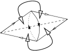
Figure 56: A two-tetrahedron triangulation of $\mathbb{R}P^{3}$

Finally, Figure 57 illustrates a two-tetrahedron triangulation of the lens space $L(3,1)$. Two tetrahedra are joined along three faces with an internal vertex of degree two, forming a triangular pillow as illustrated. The front face is then identified with the back face using a $120^{\circ}$ twist.

Figure 57: A two-tetrahedron triangulation of $L(3,1)$

Benjamin A. Burton

Department of Mathematics and Statistics

The University of Melbourne, 3010 VIC

Australia

bab@debian.org

References

- [1] Gennaro Amendola and Bruno Martelli, Non-orientable 3-manifolds of small complexity, Preprint, math.GT/0211092, November 2002.
- [2] Benjamin A. Burton, Regina (normal surface and 3-manifold topology software), http://regina.sourceforge.net/, 1999–2003.
- [3] , Structures of small closed non-orientable 3-manifold triangulations, Preprint, math.GT/0311113, November 2003.
- [4] Patrick J. Callahan, Martin V. Hildebrand, and Jeffrey R. Weeks, A census of cusped hyperbolic 3-manifolds, Math. Comp. 68 (1999), no. 225, 321–332.
- [5] Martin V. Hildebrand and Jeffrey R. Weeks, A computer generated census of cusped hyperbolic 3-manifolds, Computers and Mathematics (Cambridge, MA, 1989), Springer, New York, 1989, pp. 53–59.
- [6] Craig D. Hodgson and Jeffrey R. Weeks, Symmetries, isometries and length spectra of closed hyperbolic three-manifolds, Experiment. Math. 3 (1994), no. 4, 261–274.
- [7] William Jaco and J. Hyam Rubinstein, 0-efficient triangulations of 3-manifolds, Preprint, math.GT/0207158, July 2002.
- [8] , Layered triangulations of lens spaces, In preparation, 2003.
- [9] Bruno Martelli and Carlo Petronio, Three-manifolds having complexity at most 9, Experiment. Math. 10 (2001), no. 2, 207–236.
- [10] , A new decomposition theorem for 3-manifolds, Illinois J. Math. 46 (2002), 755–780.
- [11] , Complexity of geometric three-manifolds, Preprint, math.GT/0303249, March 2003.
- [12] Sergei V. Matveev, Tables of 3-manifolds up to complexity 6, Max-Planck-Institut für Mathematik Preprint Series (1998), no. 67, available from http://www.mpim-bonn.mpg.de/html/preprints/preprints.html.