Cut vertices in commutative graphs

Abstract

The homology of Kontsevich’s commutative graph complex parameterizes finite type invariants of odd dimensional manifolds. This graph homology is also the twisted homology of Outer Space modulo its boundary, so gives a nice point of contact between geometric group theory and quantum topology. In this paper we give two different proofs (one algebraic, one geometric) that the commutative graph complex is quasi-isomorphic to the quotient complex obtained by modding out by graphs with cut vertices. This quotient complex has the advantage of being smaller and hence more practical for computations. In addition, it supports a Lie bialgebra structure coming from a bracket and cobracket we defined in a previous paper. As an application, we compute the rational homology groups of the commutative graph complex up to rank $7$.

1 Introduction

Graph homology was introduced by Kontsevich [8, 9], who showed that it computes the homology of a certain infinite dimensional Lie algebra $c_{\infty}$, and also parameterizes invariants of certain odd dimensional manifolds. The best understood of these invariants are those associated to (rational) homology three spheres. These are known as “finite type” invariants, and are analogs of the Goussarov-Vassiliev knot invariants. Alternate constructions of these finite type invariants have been found by Le, Murakami and Ohtsuki [11], Kuperberg and Thurston [10], and Bar-Natan, Garoufalidis, Rozansky and Thurston [1].

Graph homology has a very simple definition. The degree $k$ term of the graph complex $\mathcal{G}$ is spanned (over a field of characteristic $0$) by connected, “oriented” graphs with $k$ vertices, and the boundary operator $\partial\colon\mathcal{G}_{k}\to\mathcal{G}_{k-1}$ is defined on a graph $G$ by adding together all oriented graphs which can be obtained from $G$ by collapsing a single edge. The notion of orientation is the most subtle part of the whole story (see [5, Sec. 2.3.1] for the many equivalent notions), but suffice it to say that it guarantees that $\partial^{2}=0$. Graph homology is then the homology of this complex.

Graph homology is a special case of a more general construction, where the graph complex is spanned by graphs decorated at each vertex by an element of a cyclic operad (see [5]). Ordinary graph homology corresponds to the commutative operad. Two other important examples, also studied by Kontsevich [8, 9], are obtained by using the associative operad and the Lie operad; the homology of the resulting graph complexes is closely related to the cohomology of mapping class groups of punctured surfaces and the cohomology of outer automorphisms of free groups, respectively.

Each general graph complex $\mathcal{G}$ may be considered as the primitive part of a graded Hopf algebra $\mathcal{HG}$, where the product on $\mathcal{HG}$ is given by disjoint union. In [4] we introduced a Lie bracket and cobracket on $\mathcal{HG}$. These do not form a compatible bialgebra structure on $\mathcal{HG}$, and they do not restrict to $\mathcal{G}$. However, in [4] we also introduced the subcomplex $\mathcal{B}$ of $\mathcal{G}$ spanned by connected graphs with no separating edges, and showed that the Lie bracket and cobracket do restrict to $\mathcal{B}$; furthermore, they are compatible, so give $\mathcal{B}$ a Lie bialgebra structure. In the associative and Lie cases, the subcomplex $\mathcal{B}$ is quasi-isomorphic to $\mathcal{G}$, but this is not true in the commutative case: $\mathcal{B}$ and $\mathcal{G}$ do not have the same homology.

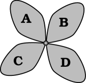
Figure 1: Schematic for a cut vertex.

In this paper we use a different approach in the commutative case to find a smaller chain complex quasi-isomorphic to $\mathcal{G}$ which carries a Lie bialgebra structure. Specifically, we consider the subcomplex $\mathcal{C}$ of $\mathcal{G}$ spanned by graphs with at least one cut vertex, where a cut vertex is defined as a vertex whose deletion disconnects the graph (Figure 1). In Section 2 we use a spectral sequence argument to prove

Theorem 1.1.

The quotient map of chain complexes $\mathcal{G}\to\mathcal{G}/\mathcal{C}$ is an isomorphism on homology.

In section 3 we recall the geometric interpretation of graph homology in terms of Outer space from [5], and reprove Theorem 1.1 from this point of view. Specifically, we show that the standard deformation retraction of Outer space onto the subspace of graphs with no separating edges extends to the Bestvina-Feign bordification of Outer Space, and we show that the image of the points at infinity consists precisely of the closure of the space of graphs with cut vertices. This deformation retraction induces a homology isomorphism on certain twisted chain complexes, which can be identified with $\mathcal{G}$ and $\mathcal{G}/{\mathcal{C}}$.

In section 4 we recall the definition of the Lie bracket and cobracket, and prove

Theorem 1.2.

The Lie bracket and cobracket on $\mathcal{HG}$ induce a compatible graded Lie bialgebra structure on $\mathcal{G}/\mathcal{C}$.

Remark. Despite the fact that the entire graph complex $\mathcal{HG}$ does not support a Lie bialgebra structure, Wee-Liang Gan [7] has recently shown that it supports a strongly homotopy Lie bialegbra structure, and that this reduces to our Lie bialgebra structure when one mods out by graphs with cut vertices.

Finally, in the last section we exploit the fact that the quotient complex $\mathcal{G}/{\mathcal{C}}$ is smaller than $\mathcal{G}$ to do some computer-aided calculations of graph homology. Specifically, the elimination of cut vertices reduces the size of the vector spaces involved by about $30\%$, allowing us to calculate graph homology up to rank 7.

2 Graphs with cut vertices

Let $G$ be an oriented graph with no separating edges. An oriented graph $H$ is said to retract to $G$ if $G$ can be obtained from $H$ by collapsing each separating edge of $H$ to a point. Denote by ${\mathcal{R}}^{G}$ the subspace of $\mathcal{G}$ spanned by all graphs $H$ which retract to $G$. Notice that according to our definitions, $\mathcal{R}^{G}$ is $1$ dimensional (with basis $G$) unless $G$ has a cut vertex. Define a boundary operator $\partial_{s}\colon{\mathcal{R}}^{G}_{k}\to{\mathcal{R}}^{G}_{k-1}$ by

$$\partial_{s}(G)=\sum_{e\,\,\,\text{separating}}G_{e}$$

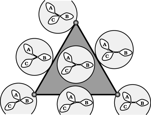
Figure 2: The simplicial realization of ${\mathcal{R}}^{v}_{+}$.

Lemma 2.1.

Let $G$ be a connected graph with at least one cut vertex, but no separating edges. Then $({\mathcal{R}}^{G},\partial_{s})$ is an acyclic complex.

Proof.

First we prove the lemma under the assumption that $G$ has no automorphisms. Fix a cut vertex $v$ of $G$, and let $c_{1},\ldots,c_{l}$ be the connected components of $G\setminus\{v\}$. Let ${\mathcal{R}}^{v}$ denote the subcomplex of ${\mathcal{R}}^{G}$ spanned by graphs whose separating edges form a tree which collapses to $v$. Grade $\mathcal{R}^{v}$ by the number of edges in the tree that collapses to $v$. We will show that the positive degree part of this subcomplex, ${\mathcal{R}}^{v}_{+}$, is the simplicial homology of a contractible simplicial complex, and that the map $\partial_{s}\colon{\mathcal{R}^{v}_{1}\to\mathcal{R}^{v}_{0}}$ serves as an augmentation map, implying the complex is acyclic. A low degree example is given in Figure 2, which shows that the simplicial realization of ${\mathcal{R}^{v}_{+}}$ where $v$ is a cut vertex that cuts the graph into three components is in fact a $2$-simplex. Notice that face maps correspond exactly to collapsing edges. Finally one needs to consider orientation. One notion of orientation for commutative graphs is an orientation of the vector space $\mathbb{R}^{\{edges\}}\oplus H_{1}(Graph;\mathbb{R})$. The first factor corresponds exactly to an orientation of the above 2-simplex, whereas the orientation of $H_{1}$ gets carried along for the ride.

In general the simplicial structure of the blow ups of a vertex is easiest to understand by considering sets of compatible partitions of $\{c_{i}\}$ as opposed to trees. If $H$ is a graph in ${\mathcal{R}}^{v}$ and $T$ is the tree in $H$ which collapses to $v$, then each edge $e$ of $T$ partitions the (preimages in $H$ of the) components $c_{i}$ into two disjoint sets. Different edges correspond to different partitions, which are compatible in the following sense: If $P_{1}=X_{1}\cup Y_{1}$ and $P_{2}=X_{2}\cup Y_{2}$, then either

$$X_{1}\subset X_{2},\,\,X_{1}\subset Y_{2},\,\,Y_{1}\subset X_{2},\,\,Y_{1}\subset Y_{2}.$$

Conversely, any set of pairwise compatible partitions determines a pair $(H,T)$ which collapses to $(G,v)$. Figure 3 shows a tree that blows up a vertex and two compatible partitions corresponding to two edges of the tree.

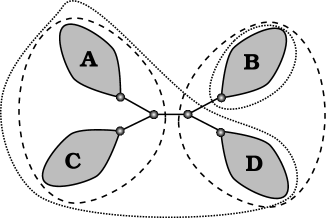
Figure 3: Two compatible partitions of the set $\{A,B,C,D\}$ corresponding to two edges of a tree.

Note that ${\mathcal{R}}^{v}_{0}$ is 1-dimensional, spanned by $G$. Thus ${\mathcal{R}}^{v}$ is the augmented chain complex of a simplicial complex whose vertices are partitions of the set $\{c_{1},\ldots,c_{l}\}$. A set of $k+1$ partitions forms a $k$-simplex if partitions in the set are pairwise compatible. The partition $P$ separating $c_{1}$ from all other components is compatible with every other set of partitions; thus this simplicial complex is a cone on the vertex $P$, and is therefore contractible. Thus the augmented chain complex $({\mathcal{R}}^{v},\partial_{s})$ is acyclic.

If we grade the entire complex $({\mathcal{R}}^{G},\partial_{s})$ by the number of edges in the forest formed by all separating edges, then it is the tensor product of the complexes $({\mathcal{R}}^{v},\partial_{s})$ for cut vertices $v$ of $G$. Thus ${\mathcal{R}}^{G}$ is acyclic.

Now let us return to the general case when the graph has a nontrivial automorphism group. Let $\widehat{\mathcal{R}}^{G}$ be the chain complex of graphs obtained from ${\mathcal{R}}^{G}$ by distinguishing all edges and vertices in each graph. (This kills off automorphisms.) Note that $Aut(G)$ acts on $\widehat{\mathcal{R}}^{G}$, and that $\widehat{\mathcal{R}}^{G}/Aut(G)\cong{\mathcal{R}}^{G}$. Over the rationals, finite groups have no homology, a fact which implies that the chain complexes $\widehat{\mathcal{R}}^{G}$ and ${\mathcal{R}}^{G}$ are rationally quasi-isomorphic. Now we are back in the case when graphs have no automorphisms, and we are done. ∎

Theorem 2.2.

The subcomplex $\mathcal{C}$ of $\mathcal{G}$ spanned by graphs with at least one cut vertex is acyclic.

Proof.

Filter $\mathcal{C}$ by the number of separating edges in the graph; i.e. let $\mathcal{F}_{p}\mathcal{C}$ be the subcomplex of $\mathcal{C}$ spanned by graphs with at most $p$ separating edges. Then

$$\mathcal{F}_{0}\mathcal{C}\subset\mathcal{F}_{1}\mathcal{C}\subset\mathcal{F}_{2}\mathcal{C}\ldots.$$

The boundary operator $\partial\colon\mathcal{C}_{k}\to\mathcal{C}_{k-1}$ is the sum of two boundary operators $\partial_{s}$ and $\partial_{ns}$, where $\partial_{s}$ collapses only separating edges, and $\partial_{ns}$ collapses only non-separating edges. These two boundary operators make $\mathcal{C}$ into the total complex of a double complex $E^{0}$, where $E^{0}_{p,q}=\mathcal{F}_{p}(\mathcal{C}_{p+q})$, the vertical arrows are given by $\partial_{s}$ and the horizontal arrows by $\partial_{ns}$:

$$\begin{matrix}&\downarrow&&\downarrow\\ \leftarrow&\mathcal{F}_{p}(\mathcal{C}_{p+q-1})&\buildrel\partial_{ns}\over{\leftarrow}&\mathcal{F}_{p}(\mathcal{C}_{p+q})&\leftarrow\\ &\ \ \downarrow_{\partial_{s}}&&\ \ \downarrow_{\partial_{s}}\\ \leftarrow&\mathcal{F}_{p-1}(\mathcal{C}_{p+q-2})&\buildrel\partial_{ns}\over{\leftarrow}&\mathcal{F}_{p-1}(\mathcal{C}_{p+q-1})&\leftarrow\\ &\downarrow&&\downarrow\\ \end{matrix}$$

Note that a graph in $\mathcal{F}_{p}(\mathcal{C})$ has at least $p+1$ vertices, so that $E^{0}_{p,q}=\mathcal{F}_{p}(\mathcal{C}_{p+q})=0$ for $q<1$, and the double complex is a first quadrant double complex.

We consider the spectral sequence associated to the vertical filtration of this double complex. This spectral sequence converges to the homology of the total complex $\mathcal{C}$. The $E^{1}_{p,q}$ term is equal to $H_{p}(E^{0}_{*,q},\partial_{s})$, i.e. the $p$-th homology of the $q$-th column.

For each $q$, the column $E^{0}_{*,q}$ breaks up into a direct sum of chain complexes $E^{G}_{*}$, one for each graph $G$ with $q$ vertices (at least one of which is a cut vertex) and no separating edges. A graph in $\mathcal{F}_{p}(\mathcal{C}_{p+q})$ is in $E^{G}_{*}$ if $G$ is the result of collapsing all of its separating edges, i.e. $E^{G}_{*}={\mathcal{R}}^{G}$. By Lemma 2.1, ${\mathcal{R}}^{G}$ has no homology, so that $E^{1}_{p,q}=0$ for all $p$ and $q$, and the complex $\mathcal{C}$ is acyclic. ∎

Theorem 1.1 now follows immediately by the long exact homology sequence of the pair $(\mathcal{G},\mathcal{C})$.

3 Geometric Interpretation, in terms of Outer Space

In this section we will sketch a geometric proof of the main theorem. This proof relies on the identification of the graph homology chain complex with a twisted relative chain complex for Outer space, as described in [5], and also on a generalization of the Borel-Serre bordification of Outer space defined by Bestvina and Feighn [2]. A similar generalization is mentioned as a remark in their paper, but details of proofs are not worked out.

Recall that Outer space $X_{n}$ is a topological space which parameterizes finite metric graphs with (free) fundamental group of rank $n$ (see [12]). Outer space can be decomposed as a union of open simplices, and there are several ways to add a boundary to this space. The simplest is to formally add the union of all missing faces to obtain a simplicial complex $\overline{X}_{n}$, called the simplicial closure of Outer Space. The bordification is more subtle; it is a blown-up version of $\overline{X}_{n}$, which we will denote $\widehat{X}_{n}$. The interiors of $\overline{X}_{n}$ and $\widehat{X}_{n}$ are both homeomorphic to $X_{n}$, and the action of $Out(F_{n})$ extends to the boundaries $\partial\overline{X}_{n}$ and $\partial\widehat{X}_{n}$. There is a natural quotient map $q\colon\widehat{X}_{n}\to\overline{X}_{n}$, which is a homeomorphism on the interiors and in general has contractible point inverses.

In [5] we showed that the subcomplex ${\mathcal{G}}^{(n)}$ of the graph complex $\mathcal{G}$ spanned by graphs with fundamental group of rank $n$ can be identified with the relative chains on $(\overline{X}_{n},\partial\overline{X}_{n})$, twisted by the non-trivial determinant action of $Out(F_{n})$ on ${\mathbb{R}}$. Blowing up the boundary does not change this picture; ${\mathcal{G}}^{(n)}$ is also identified with the relative chains on $(\widehat{X}_{n},\partial\widehat{X}_{n})$, twisted by the same non-trivial action of $Out(F_{n})$ on ${\mathbb{R}}$.

In this section we define an equivariant deformation retraction $\widehat{X}_{n}\to\widehat{Y}_{n}$, where $Y_{n}$ is the subspace of $X_{n}$ consisting of graphs with no separating edges, and $\widehat{Y}_{n}$ denotes the closure of $Y_{n}$ in $\widehat{X}_{n}$. The image of $\partial\widehat{X}_{n}$ under this retraction, denoted $\widehat{Z}_{n}$, is the union of $\partial\widehat{Y}_{n}$ and the set of graphs with a cut vertex but no separating edges. The deformation retraction induces an isomorphism

$$C_{*}(\widehat{X}_{n},\partial\widehat{X}_{n})\otimes_{Out(F_{n})}{\mathbb{R}}\cong C_{*}(\widehat{Y}_{n},\widehat{Z}_{n})\otimes_{Out(F_{n})}{\mathbb{R}}.$$

Tracing through the identification of $C_{*}(\widehat{X}_{n},\partial\widehat{X}_{n})\otimes_{Out(F_{n})}{\mathbb{R}}$ with ${\mathcal{G}}^{(n)},$ we see that the chains

$$C_{*}(\widehat{Y}_{n},\widehat{Z}_{n})\otimes_{Out(F_{n})}{\mathbb{R}}$$

are identified with ${\mathcal{G}}^{(n)}_{ns}/{\mathcal{C}}^{(n)}_{ns}$, where the subscript $ns$ denotes the subcomplex spanned by graphs with no separating edges. Since all graphs with separating edges also have cut vertices, this is naturally isomorphic to ${\mathcal{G}}^{(n)}/{\mathcal{C}}^{(n)}$. This completes the sketch of the proof of Theorem 1.1, modulo the definition of the bordfication and the retraction. The remainder of the section is devoted to just that.

It has long been known that $Y_{n}$ is an equivariant deformation retract of $X_{n}$, but the deformation retraction, which uniformly shrinks all separating edges while uniformly expanding all other edges, does not extend to $\overline{X}_{n}$. One can see this even for $n=2$ by considering the 2-simplex corresponding to the “barbell” graph (see Figure 4). The deformation retraction sends each horizontal slice linearly onto the bottom edge of the triangle, so that the deformation cannot be extended continuously to the top vertex of the closed triangle.

This difficulty can be resolved by blowing up the vertex of the triangle to a line, which records the (constant) ratio of the lengths of the two loops of the “barbell” graph along a geodesic in $X_{2}$ coming into the vertex (see Fig. 4). This is the idea of the Borel-Serre bordification $\widehat{X}_{n}$. Similar ideas are also used in the Fulton-MacPherson and Axelrod-Singer compactifications of configuration spaces of points in a manifold.

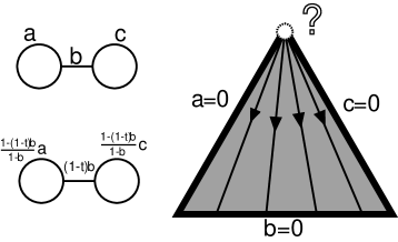
Figure 4: Why the simplicial closure doesn’t work.

To describe $\widehat{X}_{n}$ in general, we need the notion of a core graph, which is defined to be a (not necessarily connected) graph with no separating edges and no vertices of valence 0 or 1. Every graph has a unique maximal core subgraph, called its core.

A point in $X_{n}$ is a marked, nondegenerate metric graph of rank $n$ with total volume $1$, where “nondegenerate” means no edge is assigned the length $0$. In the bordification $\widehat{X}_{n}$, we allow edges of a core subgraph to have length $0$, but in this case there is a secondary metric, also of volume 1, given on the core subgraph. The secondary metric may also be zero on a smaller core subgraph, in which case there is a third metric of volume 1 on that core subgraph, etc.

In general, a point of $\widehat{X}_{n}$ consists of marked metric graph $\Gamma_{0}$ and a properly nested (possibly empty) sequence

$$\Gamma_{1}\supset\Gamma_{2}\supset\ldots\supset\Gamma_{k}$$

of core subgraphs of $\Gamma_{0}$. Each $\Gamma_{i}$ is equipped with a metric of volume 1; the metric on $\Gamma_{0}$ is the primary metric, the metric on $\Gamma_{1}$ the secondary metric etc. Each $\Gamma_{i}$ is the subgraph of $\Gamma_{i-1}$ spanned by all edges of length $0$, and the chain is nondegenerate in the sense that every edge of $\Gamma_{0}$ has non-zero length in exactly one $\Gamma_{i}$. The space $\widehat{X}_{n}$ is stratified as a union of open cells; the dimension of the cell containing $x=(\Gamma_{0}\supset\Gamma_{1}\supset\ldots\supset\Gamma_{k})$ is $e(\Gamma_{0})-k-1$, where $e(\Gamma_{0})$ is the number of edges of $\Gamma_{0}$.

This construction is illustrated for $n=2$ in Fig. 5. In this figure, the number of circles surrounding an edge length corresponds to the hierarchy of metrics. A sequence of graphs on which the volume of a core subgraph is shrinking to zero will approach a point on the boundary which depends on the relative lengths of edges in the core subgraph. If the metric is shrinking uniformly on the core subgraph, then the limit is the graph whose primary metric vanishes on the core subgraph, and where the secondary metric on the core subgraph is a rescaled version of the metric restricted to the shrinking core subgraph. If parts of the core subgraph are shrinking at a faster rate than others, the sequence will land in a face of higher codimension.

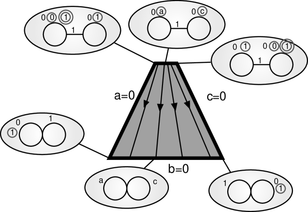
Figure 5: The deformation retraction on a cell of the bordification.

Bestvina and Feighn prove the following theorem.

Theorem 3.1 (Bestvina-Feighn).

$\widehat{Y}_{n}$ is contractible, and the $Out(F_{n})$ action on the interior extends to the whole space.

The following theorem shows that $\widehat{X}_{n}$ is also contractible, and identifies the image of the boundary $\partial\widehat{X}_{n}$.

Theorem 3.2.

$\widehat{X}_{n}$ equivariantly deformation retracts onto $\widehat{Y}_{n}$. Under this retraction, the image $\widehat{Z}_{n}$ of $\partial\widehat{X}_{n}$ is the union of $\partial\widehat{Y}_{n}$ with the set of graphs in the interior $Y_{n}$ which have a cut vertex.

Proof.

Let $x=(\Gamma_{0}\supset\ldots\supset\Gamma_{k})$ be a point in $\widehat{X}_{n}$. We define an equivariant deformation retraction $\phi(x,t)$ as follows.

If $\Gamma_{1}$ is not the maximal core of $\Gamma_{0}$, then the deformation retraction $\phi$ changes the metric on $\Gamma_{0}$ by uniformly shrinking all separating edges and rescaling the primary metric on the rest of the graph by a global factor to retain total volume 1. The metrics on $\Gamma_{k}$ for $k\geq 1$ are not affected. If, on the other hand, $\Gamma_{1}$ is the maximal core of $\Gamma_{0}$, then the deformation retraction shrinks the separating edges in $\Gamma_{0}$ (i.e. it shrinks $\Gamma_{0}\setminus\Gamma_{1}$) while simultaneously blowing up the initially degenerate $\Gamma_{1}$ by an appropriate factor in the primary metric. In other words, $\Gamma_{1}$ immediately disappears from the filtration. The metrics on $\Gamma_{i}$ for $i\geq 2$ are not affected.

We now give an explicit formula for $\phi(x,t)$. Let $m_{i}$ denote the metric on $\Gamma_{i}$, let $S$ denote the set of separating edges in $\Gamma_{0}$, and let $(\Gamma_{i})_{S}$ be the image of $\Gamma_{i}$ under the map which collapses each edge in $S$ to a point. The formula depends on whether $m_{0}(S)=1$ (i.e. $\Gamma_{1}$ is the entire core of $\Gamma_{0}$) or $m_{0}(S)<1$.

If $m_{0}(S)<1$, then for $0<t<1$ we have $\phi(x,t)=(\Gamma_{0}\supset\Gamma_{1}\supset\ldots\supset\Gamma_{k})$, where the new metric $n_{i}$ on $\Gamma_{i}$ is given by

$$n_{i}(e)=\begin{cases}(1+t({{m_{0}(S)}\over{1-m_{0}(S)}}))\,m_{0}(e)&i=0,e\in\Gamma_{0}\setminus S\\ (1-t)\,m_{0}(e)&i=0,e\in S\\ m_{i}(e)&i>0,e\in\Gamma_{i}\\ \end{cases}$$

For $t=1$, $\phi(x,t)=((\Gamma_{0})_{S}\supset(\Gamma_{1})_{S}\supset\ldots\supset(\Gamma_{k})_{S})$, where $(\Gamma_{i})_{S}$ is the image of $\Gamma_{i}$ under the map which collapses each edge in $S$ to a point. The length of each edge $e\in(\Gamma_{0})_{S}$ is $({1\over{1-m_{0}(S)}})\,m_{0}(e)$, and the length of $e\in(\Gamma_{i})_{S}$ is $m_{i}(e)$.

If $m_{0}(S)=1$, then for $0<t<1$ we have $\phi(x,t)=(\Gamma_{0}\supset\Gamma_{2}\supset\ldots\supset\Gamma_{k})$, where the new metric $n_{i}$ on $\Gamma_{i}$ is given by

$$n_{i}(e)=\begin{cases}(1-t)m_{0}(e)+tm_{1}(e)&i=0,e\in\Gamma_{0}\setminus S\\ (1-t)m_{0}(e)&i=0,e\in S\\ m_{i}(e)&i>1,e\in\Gamma_{i}\\ \end{cases}$$

If $t=1$, then $\phi(x,t)=((\Gamma_{1})_{S}\supset(\Gamma_{2})_{S}\supset\ldots\supset(\Gamma_{k})_{S})$, where the length of each edge $e$ of $(\Gamma_{i})_{S}$ is equal to $m_{i}(e)$ for all $i$.

The deformation retraction restricted to a cell in the case $n=2$ is pictured in Figure 5. The top line corresponds to graphs with a degenerate core, and the flow pushes them into strata of $\widehat{X}_{n}$ of one higher dimension. Everywhere else, the flow stays within strata until $t=1$, when the dimension of the stratum may decrease.

The fact that points in $\partial\widehat{X}_{n}$ land in $\widehat{Z}_{n}$ is clear. Now we attack the question of continuity. For this, it will be convenient to fix a metric on each closed cell of $\hat{X}_{n}$. Every top dimensional cell is associated to a marked trivalent graph, $\Gamma$. Call such a closed cell $\hat{\Sigma}_{\Gamma}$. Let $C$ be a core subgraph of $\Gamma$. For every point of $\hat{\Sigma}_{\Gamma}$, $C$ has a level, which is the unique $i$, such that the metric $m_{i}$ is defined on $C$ and is not identically zero on $C$. (If we are looking at a point on $\partial\hat{\Sigma}_{\Gamma}$ where a subforest has been contracted, then the level is defined for the image of $C$ under this contraction.)

Let $x,x^{\prime}$ be two points in $\hat{\Sigma}_{\Gamma}$, and let $C\subset\Gamma$ be a core subgraph and let $l,l^{\prime}$ be the levels of $C$ in $x$ and $x^{\prime}$. Then define

$$d_{C}(x,x^{\prime})=\sum_{e\in E(C)}\left|\frac{m_{l}(e)}{m_{l}(C)}-\frac{m^{\prime}_{l^{\prime}}(e)}{m_{l^{\prime}}^{\prime}(C)}\right|.$$

Then the metric on on $\hat{\Sigma}_{\Gamma}$ is defined to be

$$d(x,x^{\prime})=\sum_{C\subset\Gamma}d_{C}(x,x^{\prime}),$$

where the sum is over all core subgraphs of $\Gamma$ including $\Gamma$ itself. That this metric generates the appropriate topology follows from Lemma 2.3 of [2].

To show that $\phi$ is continuous it suffices to show that on each closed cell $\hat{\Sigma}_{\Gamma}$, the functions $\phi(x_{0},t)$ are equicontinuous as a family indexed by $x_{0}$ and that each function $\phi(x,t_{0})$ is continuous as a function of $x$. Recall that equicontinuous means that for every $\epsilon>0$ there exists a $\delta>0$ such that $|t-s|<\delta\Rightarrow\forall x_{0}(d(\phi(x_{0},t),\phi(x_{0},s))<\epsilon)$.

The continuity of $\phi(x_{0},t)$ as a function of $t$ is clear except when $x_{0}$ represents $\Gamma\supset\Gamma_{1}\supset\ldots$, and $\Gamma_{1}$ is the maximal core of $\Gamma$. However, here too $\phi$ is continuous, since by construction of $\widehat{X}_{n}$, $x_{0}:=\underset{t\to 0}{\lim}\,\phi(x_{0},t)$. Note that as functions of $t$, the formula for how the length of each edge changes is a linear map with coefficients bounded by $1$. This ensures that the family of functions is equicontinuous, since

$$d(\phi(x_{0},t),\phi(x_{0},s)) =\sum_{C\subset G}d_{C}(\phi(x_{0},t),\phi(x_{0},s))$$

$$\leq\sum_{C\subset G}\sum_{e\in E(C)}|t-s|$$

$$\leq N\cdot|t-s|$$

where $N$ is a constant independent of $x_{0}$.

Now we wish to show continuity in $x$. Clearly $\phi$ is continuous on the interiors of cells, so we need to consider what happens as we approach the boundary. It will be simpler to analyze what happens as we go from a cell $\Sigma$ to a codimension one stratum $B$. Suppose $\Sigma$ corresponds to the sequence of graphs $\Gamma_{0}\supset\Gamma_{1}\supset\ldots\supset\Gamma_{k}$. Then the face $B$ comes from one of two processes. Either it corresponds to contracting an edge $e$: $(\Gamma_{0})_{e}\supset(\Gamma_{1})_{e}\supset\ldots\supset(\Gamma_{k})_{e}$, or it corresponds to refining the filtration by inserting a new core graph $C$: $\Gamma_{0}\supset\ldots\Gamma_{i}\supset$C$\supset\Gamma_{i+1}\supset\ldots\supset\Gamma_{k}$. For every point $x$ on $B$, there is a canonical path, $P_{x}$, into $\Sigma$. In the first case, it is defined by expanding the contracted edge in the metric that makes sense, shrinking the other edges in that metric to maintain total volume $1$. In the second case, the core $C$ is expanded from length zero in the $i$th metric, using a scaled version of the metric that had been defined on $C$. The other edges in $\Gamma_{i}$ are scaled down to maintain total volume $1$.

We will show that, for every $\epsilon>0$ there is a $\delta$ such that

$$\forall x\in B\forall y\in P_{x}(d(x,y)<\delta\Rightarrow d(\phi(x,t_{0}),\phi(y,t_{0}))<\epsilon).$$

This condition will be called boundary equicontinuity. This is sufficient to ensure continuity. For example, to show continuity at a point $z$ on a codimension $2$ face, let $x$ be a nearby point in the top cell. Let $y$ be the projection onto one of the nearby codimension $1$ faces (i.e. $x\in P_{y}$), and $z^{\prime}$ the projection onto the codimension 2 face (i.e. $y\in P_{z^{\prime}}$). Thus if $x$ is sufficiently close to $z$, then $x,y$ are close, $y,z^{\prime}$ are close, and $z,z^{\prime}$ are close. Then

$$d(\phi(x,t_{0}),\phi(z,t_{0}))\leq\\ d(\phi(x,t_{0}),\phi(y,t_{0}))+d(\phi(y,t_{0}),\phi(z,t_{0}))+d(\phi(z,t_{0}),\phi(z^{\prime},t_{0})),$$

and by the boundary equicontinuity hypothesis we can make the first two terms uniformly $<\epsilon/3$ and by continuity on the interior of cells at $z$ we can bound the last term by $\epsilon/3$.

So now let us show boundary equicontinuity. Let $x$ be an interior point and $x^{\prime}$ be nearby on a codimension $1$ face, such that $x\in P_{x^{\prime}}$.

As mentioned above, in one case, $x^{\prime}=(\Gamma_{0})_{e}\supset\ldots\supset(\Gamma_{k})_{e}$, where the metric on edges is unchanged except in the image of the (unique) graph $\Gamma_{i}$ of the filtration in which $e$ has non-zero length; in $(\Gamma_{i})_{S}$, edges are scaled by ${1\over{1-m_{i}(e)}}$. The fact that $x$ is close to $x^{\prime}$ means that $m_{i}(e)$ is very small.

In the other case $x^{\prime}=\Gamma_{0}\supset\ldots\supset\Gamma_{i}\supset C\supset\Gamma_{i+1}\supset\ldots\supset\Gamma_{k}$. The metric on $C$ is ${1\over m_{i}(C)}$ times the restriction of $m_{i}$ to $C$. The metric on $\Gamma_{i}$ is $0$ on $C$, and ${1\over{1-m_{i}(C)}}\,m_{i}$ on edges not in $C$. The fact that $x$ is close to $x^{\prime}$ means that $m_{i}(C)$ is small.

It is now routine to check that $\phi(x,t)$ is uniformly close to $\phi(x^{\prime},t)$ in all cases. As an example, we check one of the more complicated cases, when $x^{\prime}=\Gamma_{0}\supset C\supset\Gamma_{1}\supset\ldots\supset\Gamma_{k}$, where $C$ is the core of $\Gamma_{0}$. Let $|e|$ denote the primary metric on $x$. Then $|S|+|C|=1$. The primary length of $e$ in $x^{\prime}$ is $0$ if $e\in C$ and $|e|/|S|$ if $e\in S$. The secondary length of $e\in C$ in $x^{\prime}$ is $|e|/|C|$. We now compute $\phi(x,t)$ and $\phi(x^{\prime},t)$ using the formulas above.

Note that $\Gamma_{1}$ is not the core of $\Gamma_{0}$, so

$$\phi(x,t)=\big{(}\Gamma_{0}\supset\Gamma_{1}\supset\ldots\supset\Gamma_{k}\big{)},$$

for $0<t<1$. The primary length of $e$ is

$$|e|_{\phi(x,t)}=\begin{cases}(1-t)|e|&e\in S\\ (1+t{|S|\over{1-|S|}})|e|=((1-t)|C|+t){|e|\over|C|}&e\in C\end{cases}$$

On the other hand, $C$ is the core of $\Gamma_{0}$ so again

$$\phi(x^{\prime},t)=\big{(}\Gamma_{0}\supset\Gamma_{1}\supset\ldots\supset\Gamma_{k}\big{)},$$

for $0<t<1$. Now the primary length of $e$ is

$$|e|_{\phi(x^{\prime},t)}=\begin{cases}(1-t){|e|\over|S|}&e\in S\\ t{|e|\over|C|}&e\in C\end{cases}$$

Now, to show that equicontinuouity at this boundary, we calculate distances. First, we claim that $d(x,x^{\prime})=d_{\Gamma_{0}}(x,x^{\prime})$. So let $D\neq\Gamma_{0}$ be a core subgraph of $\Gamma_{0}$. Then $D\subset C$. If the primary metric of $x$ vanishes on $D$, then the first nonvanishing metric is the same for both $x$ and $x^{\prime}$, and so $d_{D}(x,x^{\prime})=0$. If $D$ does not vanish in $x$’s primary metric, $D$ vanishes in the primary metric of $x^{\prime}$, and is rescaled in the secondary metric: $m_{2}^{\prime}|_{D}=m_{1}|_{D}\cdot\frac{1}{|C|}$. Then

$$d_{D}(x,x^{\prime}) =\sum_{e\in E(D)}\left|\frac{m_{1}(e)}{m_{1}(D)}-\frac{m^{\prime}_{2}(e)}{m^{\prime}_{2}(D)}\right|$$

$$=\sum_{e\in E(D)}\left|\frac{m_{1}(e)}{m_{1}(D)}-\frac{m_{1}(e)\cdot|C|^{-1}}{m_{1}(D)\cdot|C|^{-1}}\right|$$

$$=0$$

So we have

$$d(x,x^{\prime}) =d_{\Gamma_{0}}(x,x^{\prime})$$

$$=\sum_{e\in E(C)}||e|-|e|^{\prime}|+\sum_{e\in E(S)}||e|-|e|^{\prime}|$$

$$=\sum_{e\in E(C)}||e|-0|+\sum_{e\in E(S)}||e|-\frac{|e|}{|S|}|$$

$$=|C|+|S||1-1/|S||$$

$$=2|C|.$$

On the other hand

$$\begin{split}d(\phi(x,t_{0}),\phi(x^{\prime},t_{0}))&=d_{\Gamma_{0}}(\phi(x,t_{0}),\phi(x^{\prime},t_{0}))\\ &=\sum_{e\in E(S)}|(1-t_{0})|e|-(1-t_{0})\frac{|e|}{|S|}|\\ &\phantom{=dummy}+\sum_{e\in E(C)}|(1-t_{0})|C|+t)\frac{|e|}{|C|}-t_{0}\frac{|e|}{|C|}|\\ &=(1-t_{0})(|S||1-1/|S||+|C||)\\ &=2(1-t_{0})|C|\end{split}$$

Thus we can take $\delta=\frac{\epsilon}{1-t_{0}}$, which is independent of $x$.

∎

4 Lie bialgebra structure on $\mathcal{G}/\mathcal{C}$

Recall that $\mathcal{HG}$ denotes the Hopf algebra spanned by all oriented graphs (not necessarily connected). In this section, we will show that the Lie bracket and cobracket on $\mathcal{HG}$ introduced in [4] induce a Lie bracket and cobracket on $\mathcal{G}/\mathcal{C}$, and that these are compatible on $\mathcal{G}/\mathcal{C}$.

We first recall the definition of the Lie bracket. Let $G$ be a graph, and let $x$ and $y$ be half-edges of $G$, terminating at the vertices $v$ and $w$ respectively. Form a new graph as follows: Cut the edges of $G$ containing $x$ and $y$ in half and glue $x$ to $y$ to form a new edge $xy$, with vertices $v$ and $w$. If $y$ was not the other half of $x$ (i.e. $y\neq\bar{x}$), there are now two “dangling” half-edges $\bar{x}$ and $\bar{y}$. Glue these to form another new edge $\bar{x}\bar{y}$. Finally, collapse the edge $xy$ to a point. We say the resulting graph, denoted $G_{xy}$, is obtained by contracting the half-edges $x$ and $y$.

Recall that the Hopf algebra product $G\cdot H$ is the disjoint union of $G$ and $H$, with appropriate orientation. The bracket of $G$ and $H$ is defined to be the sum of all graphs obtained by contracting a half-edge of $G$ with a half-edge of $H$ in $G\cdot H$:

$$[G,H]=\sum_{x\in G,y\in H}(G\cdot H)_{xy}.$$

For more information about the bracket, we refer to [4]; there we show, e.g., that there is a second boundary operator on $\mathcal{HG}$, and the bracket measures how far this boundary operator is from being a derivation.

If $x$ and $y$ belong to separating edges of $G$ and $H$, then $(G\cdot H)_{xy}$ will not be connected, even if $G$ and $H$ are connected. Thus the bracket on $\mathcal{HG}$ does not restrict to a bracket on $\mathcal{G}.$ It does restrict to a bracket on the subcomplex of $\mathcal{G}$ spanned by graphs with no separating edges, but that subcomplex is not quasi-isomorphic to $\mathcal{G}$. However, we will show that it does induce a well-defined bracket on $\mathcal{G}/\mathcal{C}$. The quotient $\mathcal{G}/\mathcal{C}$ has as basis the cosets $G+\mathcal{C}$, where $G$ is connected with no cut vertices. We define the bracket on basis elements by $[G+\mathcal{C},H+\mathcal{C}]=[G,H]+\mathcal{C}$, where $G$ and $H$ are connected with no cut vertices. To see that this is well-defined, we need the following lemma.

Lemma 4.1.

If $G,H\neq 0$ are connected and have no cut vertices, then each term $(G\cdot H)_{xy}$ of $[G,H]$ is connected and has no cut vertices. If $G$ or $H$ has a cut vertex, then so does each term $(G\cdot H)_{xy}$.

Proof.

Since we are restricting to nonzero graphs, we may assume there are no loops at any vertices. A graph without loops is connected with no cut vertices if and only if there are at least two disjoint paths between every pair of vertices. Let $v$ be the vertex of $G$ adjacent to $x$ and $\bar{v}$ the vertex adjacent to $\bar{x}$; similarly, let $w,\bar{w}$ be the vertices of $H$ adjacent to $y,\bar{y}$. Choose a path $\alpha$ in $G$ from $v$ to $\bar{v}$ which does not contain $x$, and $B$ a path in $H$ from $w$ to $\bar{w}$ which does not contain $y$.

If $a$ and $b$ are two vertices of $G$, and one of the two disjoint paths between them contains $x\bar{x}$, then we can construct a second disjoint path in $(G\cdot H)_{xy}$ by replacing $x\bar{x}$ by $B$. Similarly, if $a$ and $b$ are in $H$, we can replace a path containing $y\bar{y}$ by $\alpha$. If $a$ is in $G$ and $b$ is in $H$, then disjoint paths can be constructed as follows: To make the first path, join $a$ to the image of $v$ and the (identical) image of $w$ to $b$; the second path is obtained by joining $a$ to $\bar{v}$, then going across $\bar{x}\bar{y}$, then joining $\bar{w}$ to $b$.

If a vertex is a cut vertex in $G$, its image is a cut vertex in $(G\cdot H)_{xy}$. ∎

Corollary 4.2.

The bracket induces a well-defined bracket on $\mathcal{G}/\mathcal{C}$.

Proof.

The only subtlety here is that the bracket of two graphs with separating edges (and hence cut vertices) may not be connected. Let $C_{1},C_{2}\in\mathcal{C}$, and let $\mathcal{HC}$ be the subspace of $\mathcal{HG}$ spanned by graphs with cut vertices. Then $[G+C_{1},H+C_{2}]=[G,H]+[G,C_{2}]+[C_{1},H]+[C_{1},C_{2}]\in[G,H]+\mathcal{HC},$ by the lemma. We then appeal to the natural isomorphism

$$(\mathcal{G}+\mathcal{HC})/\mathcal{HC}\cong\mathcal{G}/\mathcal{C}$$

to identify $[G+C_{1},H+C_{2}]$ with $[G,H]$ in $\mathcal{G}/\mathcal{C}$. ∎

Remark 4.3.

The Lemma shows that the bracket restricts to the subspace of $\mathcal{G}$ spanned by graphs with no cut vertices. However, that subspace is not a subcomplex, as the boundary map does not restrict. This is the reason we are using the quotient complex $\mathcal{G}/\mathcal{C}$.

The cobracket $\mathcal{HG}\to\mathcal{HG}\otimes\mathcal{HG}$ is defined as follows. We say a pair $\{x,y\}$ of half-edges of a graph $G$ is separating if the number of components of $G_{xy}$ is greater than that of $G$. If $G$ is connected, define

$$\theta(G)=\sum_{\{x,y\}\,\,\text{separating}}A\otimes B+(-1)^{a}B\otimes A,$$

where $G_{xy}=A\cdot B$, and $a$ is the number of vertices of $A$. This gives the coproduct on primitive elements, and extends to all elements in a standard way (see [4]). We have

Lemma 4.4.

Let $\{x,y\}$ be a separating pair of half-edges in an oriented graph $G$, with $G_{xy}=A\cdot B$. If $G$ has a cut vertex, then at least one of $A$ or $B$ has a cut vertex. If $G$ is connected, then both $A$ and $B$ are connected.

Proof.

The proof is straightforward. ∎

Thus the cobracket induces a cobracket on $(\mathcal{G}+\mathcal{HC})/\mathcal{HC}\cong\mathcal{G}/\mathcal{C}$ defined on a basis element $G+\mathcal{C}$, where $G$ is a connected graph with no cut vertices, by

$$\theta(G+\mathcal{C})=\sum_{\{x,y\}\,separating}(A+\mathcal{C})\otimes(B+\mathcal{C})+(-1)^{a}(B+\mathcal{C})\otimes(A+\mathcal{C}).$$

We now check that the bracket and cobracket are compatible on $\mathcal{G}/\mathcal{C}$, making $\mathcal{G}/\mathcal{C}$ into a Lie bialgebra:

Proposition 4.5.

The bracket and cobracket satisfy

$$\theta[G+\mathcal{C},H+\mathcal{C}]+[\theta(G+\mathcal{C}),H+\mathcal{C}]+(-1)^{g}[G+\mathcal{C},\theta(H+\mathcal{C})]=0,$$

where $g$ is the degree of $G$.

Proof.

Let $G+\mathcal{C}$ and $H+\mathcal{C}$ be basis elements of $\mathcal{G}/\mathcal{C}$, i.e. $G$ and $H$ are connected with no cut vertices. We compute

$$\theta[G+\mathcal{C},H+\mathcal{C}]+[\theta(G+\mathcal{C}),H+\mathcal{C}]+(-1)^{g}[G+\mathcal{C},\theta(H+\mathcal{C})]$$

$$=\theta[G,H]+[\theta(G),H]+(-1)^{g}[G,\theta(H)].$$

Because both $G$ and $H$ have no cut vertices, they also have no separating edges, so the last sum is zero by Theorem 1 of [4]. ∎

5 Calculations

In this section we present our computations of the rational homology of $\mathcal{G}^{(n)}$ for $n\leq 7$, briefly describing the algorithm, but omitting the raw code. Details for a similar algorithm can be found in [6].

The program first enumerates all trivalent graphs with no cut vertices. There is only one such graph with fundamental group of rank 2, the theta graph: two vertices connected by three edges. If we have a list of all graphs with fundamental group of rank $n-1$, we can obtain the list for rank $n$ by applying one of the following two operations to all the graphs in every possible way. The first operation takes two distinct edges of the graph, subdivides them by adding a new vertex at the middle of each, and adds a new edge between the two new vertices. The second operation adds two new vertices in the interior of a single edge and connects the two new vertices by a new edge. It is not hard to see that if $G$ has no cut vertices, then it can be obtained from a lower rank graph which also has no cut vertices using one of these two operations.

The same graph will be listed several times. To eliminate the duplications, we transform each new graph into a normal form; two graphs in normal form are isomorphic if and only if they are identical. The graph is stored as the adjacency matrix $a_{ij}$ for $i<j$; i.e., $a_{ij}=k$ if vertex $i$ is connected to vertex $j$ by $k$ edges. The normal form of the graph is the ordering of the vertices which yields the matrix latest in the lexicographic ordering. Permutations of the vertices are listed, and the matrices are compared. The number of permutations needed is reduced by distinguishing 3 types of vertices: those contained in a multiple edge, those contained in a triangle, and the rest. Only vertices of the same type need to be permuted among themselves.

Next, we enumerate all graphs of valence 3 or higher, with no cut vertices and with fundamental group of rank at most 7, by successively contracting edges of the trivalent graphs. Cut vertices may develop during this process; in this case the graph is discarded. Then we examine each graph to see whether it has any orientation-reversing automorphisms, and if so, discard it. A graph with an orientation-reversing automorphism is zero in the graph complex since such a graph is equal to minus itself and the base field is of characteristic zero.

Finally, we compute the matrix of the boundary map

$$\partial(G)=\sum_{e}G_{e}$$

by transforming each contracted graph $G_{e}$ into normal form and comparing it to the list of lower rank graphs. The output of the program is a sparse matrix; its rank was computed by simple Gaussian elimination in the case of the smaller matrices and by the software package scilab in the case of the largest ones.

Recall that $\mathcal{G}^{(n)}$ denotes the subcomplex of the graph complex spanned by rank $n$ graphs, and that $\mathcal{C}^{(n)}$ is the subcomplex spanned by graphs with cut vertices. We obtain the following rank $n$ quotient complexes $\mathcal{G}^{(n)}/\mathcal{C}^{(n)}$ for values of $n$ less than $8$:

$\mathcal{G}^{(3)}/\mathcal{C}^{(3)}$:

$$\begin{CD}0@>{}>{}>\underset{2}{C_{4}}@>{1}>{}>\underset{1}{C_{3}}@>{0}>{}>\underset{0}{C_{2}}@>{}>{}>0\end{CD}$$

$\mathcal{G}^{(4)}/\mathcal{C}^{(4)}$:

$$\setcounter{MaxMatrixCols}{13}\begin{CD}0@>{}>{}>\underset{4}{C_{6}}@>{3}>{}>\underset{3}{C_{5}}@>{0}>{}>\underset{0}{C_{4}}@>{0}>{}>\underset{1}{C_{3}}@>{1}>{}>\underset{1}{C_{2}}@>{}>{}>0\end{CD}$$

$\mathcal{G}^{(5)}/\mathcal{C}^{(5)}$:

$$\setcounter{MaxMatrixCols}{15}\begin{CD}0@>{}>{}>\underset{14}{C_{8}}@>{12}>{}>\underset{19}{C_{7}}@>{7}>{}>\underset{12}{C_{6}}@>{5}>{}>\underset{12}{C_{5}}@>{7}>{}>\underset{10}{C_{4}}@>{3}>{}>\underset{3}{C_{3}}@>{0}>{}>\end{CD}\\ \begin{CD}\underset{0}{C_{2}}@>{}>{}>0\end{CD}$$

$\mathcal{G}^{(6)}/\mathcal{C}^{(6)}$:

$$\setcounter{MaxMatrixCols}{15}\begin{CD}0@>{}>{}>\underset{54}{C_{10}}@>{52}>{}>\underset{128}{C_{9}}@>{76}>{}>\underset{177}{C_{8}}@>{101}>{}>\underset{218}{C_{7}}@>{116}>{}>\underset{177}{C_{6}}@>{61}>{}>\underset{72}{C_{5}}@>{11}>{}>\end{CD}\\ \begin{CD}\underset{12}{C_{4}}@>{1}>{}>\underset{2}{C_{3}}@>{1}>{}>\underset{1}{C_{2}}@>{}>{}>0\end{CD}$$

$\mathcal{G}^{(7)}/\mathcal{C}^{(7)}$:

$$\setcounter{MaxMatrixCols}{13}\begin{CD}0@>{}>{}>\underset{298}{C_{12}}@>{295}>{}>\underset{1123}{C_{11}}@>{828}>{}>\underset{2388}{C_{10}}@>{1560}>{}>\underset{3530}{C_{9}}@>{1969}>{}>\underset{3362}{C_{8}}@>{1393}>{}>\end{CD}\\ \setcounter{MaxMatrixCols}{13}\begin{CD}\underset{1933}{C_{7}}@>{540}>{}>\underset{678}{C_{6}}@>{138}>{}>\underset{173}{C_{5}}@>{35}>{}>\underset{41}{C_{4}}@>{6}>{}>\underset{6}{C_{3}}@>{0}>{}>\underset{0}{C_{2}}@>{}>{}>0\end{CD}$$

The number printed under the chain group $C_{i}$ is its dimension, the number printed above the arrow $\partial_{i}\colon C_{i}\to C_{i-1}$ is its rank. Thus we have the following.

Theorem 5.1.

The rational homology $H_{i}(\mathcal{G}^{(n)})$ of the commutative graph complex is zero for all $2\leq n\leq 7$ and all $i$ except for

$$H_{2}(\mathcal{G}^{(2)})\cong{\mathbb{Q}}$$

$$H_{4}(\mathcal{G}^{(3)})\cong{\mathbb{Q}}$$

$$H_{6}(\mathcal{G}^{(4)})\cong{\mathbb{Q}}$$

$$H_{8}(\mathcal{G}^{(5)})\cong{\mathbb{Q}}^{2}$$

$$H_{10}(\mathcal{G}^{(6)})\cong{\mathbb{Q}}^{2}\qquad H_{7}(\mathcal{G}^{(6)})\cong{\mathbb{Q}}$$

$$H_{12}(\mathcal{G}^{(7)})\cong{\mathbb{Q}}^{3}\qquad H_{9}(\mathcal{G}^{(7)})\cong{\mathbb{Q}}.$$

For $2\leq n\leq 5$, the computation takes only a few minutes. For $n=6$, it took several hours of CPU time, and for $n=7$, several thousand hours, even though the elimination of graphs with cut vertices reduces the size of the computation by about 30%.

As Kontsevich realized, any metrized Lie algebra produces classes in trivalent graph homology, and so the abundance of top dimensional homology is perhaps not surprising. Indeed, these trivalent classes correspond to finite type three manifold invariants. On the other hand, the presence of two codimension $3$ classes is rather tantalizing.

The source code for the program is available in the source Folder available with the “source” for this paper on arXiv.org. Please look at the readme file first. There is also a data Folder available in the same place.

Acknowledgements. The first author was partially supported by NSF grant DMS-0305012. The third author was partially supported by NSF grant DMS-0204185. The computations were done at the NIIFI Supercomputing Centre in Budapest, Hungary. We thank Craig Jensen for pointing out several typographical errors in an earlier draft.

References

- [1] D. Bar-Natan, S. Garoufalidis, L. Rozansky and D. Thurston, The Aarhus integral of rational homology 3-spheres I: A highly nontrivial flat connection on ., Selecta Math. (N.S.) 8 (2002), no. 3, 315–319.
- [2] Mladen Bestvina and Mark Feighn, The topology at infinity of Invent. Math. 140 (2000), no. 3, 651–692
- [3] James Conant, Fusion and fission in graph complexes, Pac. J. Math., Vol. 209, No.2 (2003), 219-230.
- [4] James Conant and Karen Vogtmann, Infinitesimal operations on complexes of graphs, Math. Ann.327 (2003), no. 3, 545–573.
- [5] James Conant and Karen Vogtmann, On a theorem of Kontsevich, Algebr. Geom. Topol. 3 (2003), 1167-1224.
- [6] Ferenc Gerlits, Invariants in chain complexes of graphs, Cornell Ph.D. thesis, 2002.
- [7] Wee Liang Gan, On a theorem of Conant-Vogtmann, preprint 2004, math.QA/0404173.
- [8] Maxim Kontsevich, Formal (non)commutative symplectic geometry. The Gelfand Mathematical Seminars, 1990–1992, 173–187, Birkhäuser Boston, Boston, MA, 1993.
- [9] Maxim Kontsevich, Feynman diagrams and low-dimensional topology. First European Congress of Mathematics, Vol. II (Paris, 1992), 97–121, Progr. Math., 120, Birkh user, Basel, 1994.
- [10] Greg Kuperberg and Dylan P. Thurston Perturbative 3-manifold invariants by cut-and-paste topology, preprint 1999, UC Davis Math 1999-36, math.GT/9912167
- [11] T.Q.T. Le, J. Murakami and T. Ohtsuki, On a universal perturbative invariant of -manifolds, Topology 37-3 (1998)
- [12] Karen Vogtmann, Automorphisms of free groups and Outer Space Geometriae Dedicata, v. 94: 1–31, 2002.