A step towards holistic discretisation of stochastic partial differential equations

Abstract

The long term aim is to use modern dynamical systems theory to derive discretisations of noisy, dissipative partial differential equations. As a first step we here consider a small domain and apply stochastic centre manifold techniques to derive a model. The approach automatically parametrises subgrid scale processes induced by spatially distributed stochastic noise. It is important to discretise stochastic partial differential equations carefully, as we do here, because of the sometimes subtle effects of noise processes. In particular we see how stochastic resonance effectively extracts new noise processes for the model which in this example helps stabilise the zero solution.

1 Introduction

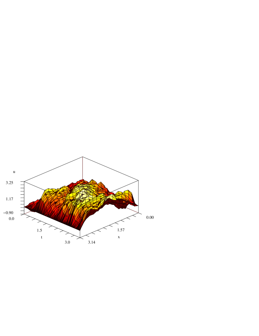
Figure 1: numerical solution over time $0<t<3$ of the spde (1) on the domain $0<x<\pi$ with stochastic forcing (2) truncated to the first seven spatial modes. Parameters: $\gamma=0$ so $u\propto\sin x$ is linearly neutral although nonlinearly stable; $\sigma=1$ for large forcing; numerically $\Delta x=\pi/16$ and $\Delta t=0.01$ .

The ultimate aim is to accurately and efficiently model numerically the evolution of stochastic partial differential equations (spdes). An example solution field $u(x,t)$, see Figure 1, shows the intricate spatio-temporal dynamics typically generated in a spde. Numerical methods to integrate stochastic ordinary differential equations are known to be delicate and subtle [9, e.g.]. We surely need to take considerable care for spdes as well [8, 20, e.g.].

An issue is that the stochastic forcing generates high wavenumber, steep variations, in structures seen in Figure 1. Stable implicit integration in time generally damps far too fast such decaying modes, yet through stochastic resonance an accurate resolution of the life-time of these modes may be important on the large scale dynamics. For example, stochastic resonance causes a high wavenumber noise to restabilise the trivial solution field $u=0$ in the simulations summarised in Figure 2. Thus we should resolve reasonably subgrid structures so that numerical discretisation with large space-time grids achieve efficiency, without sacrificing the subtle interactions that take place between the subgrid scale structures.

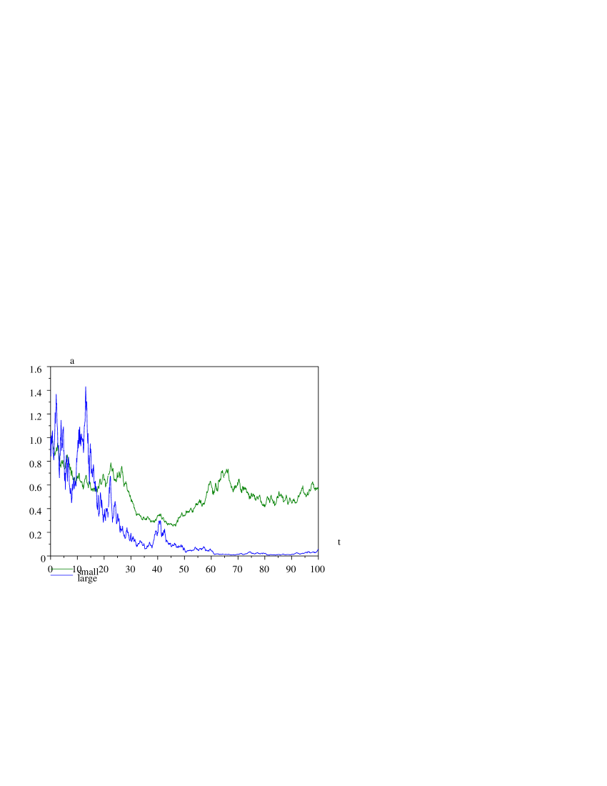
Figure 2: numerical solution of the sde model (6) with small, $\sigma=0.5$, and large, $\sigma=2$, noise. The amplitude $a$ of the $\sin x$ mode decays for large noise, but not for small. Parameters: $\gamma=-0.03$ to promote linear growth of $a$, and $\Delta t=0.1$ .

The methods of centre manifold theory are used here to begin to develop good methods for the discretisation of spdes. There is supporting centre manifold theory by Boxler [3, 4, 2] for the modelling of sdes; the centre manifold approach appears a better foundation than heuristic arguments for sdes [12, e.g.]. Further, a centre manifold approach seems to improve the discretisation of deterministic partial differential equations [15, 17, 10, 16, 18, 11]. The first step, taken here, is to demonstrate the effective modelling of subgrid scale stochastic structures.

2 Directly seek a one element model

The simplest case, and that developed here, is the modelling of a spde on just one finite size element. Consider the stochastically forced nonlinear partial differential equation

$$\frac{\partial u}{\partial t}=-u\frac{\partial u}{\partial x}+\frac{\partial^{2}u}{\partial x^{2}}+(1-\gamma)u+\sigma\phi(x,t)\quad\mbox{such that}\quad u=0\mbox{ at }x=0,\pi\,,$$ (1)

which involves advection $uu_{x}$, diffusion $u_{xx}$, reaction $(1-\gamma)u$, and noise $\phi$. In general, the forcing by $\phi(x,t)$, of strength $\sigma$, is assumed to be white noise that is delta correlated in both space and time as used in Figure 1; however, here we consider only the case

$$\phi=\phi_{2}(t)\sin 2x\,,$$ (2)

where the $\phi_{2}(t)$ is a white noise that is delta correlated in time. Note that the mode $u\propto\sin x$, when $\gamma=0$ , is linearly neutral and will form the basis of the model we seek. Thus this example of noise forcing the orthogonal $\sin 2x$ mode is expected to be representative of the case of subgrid stochastic forcing and consequent resolution of higher wavenumber modes. Many simple numerical methods, such as Galerkin projection (remembering that the domain here represents just one finite element), would completely obliterate such “high wavenumber” modes and hence completely miss subtle but important subgrid effects.

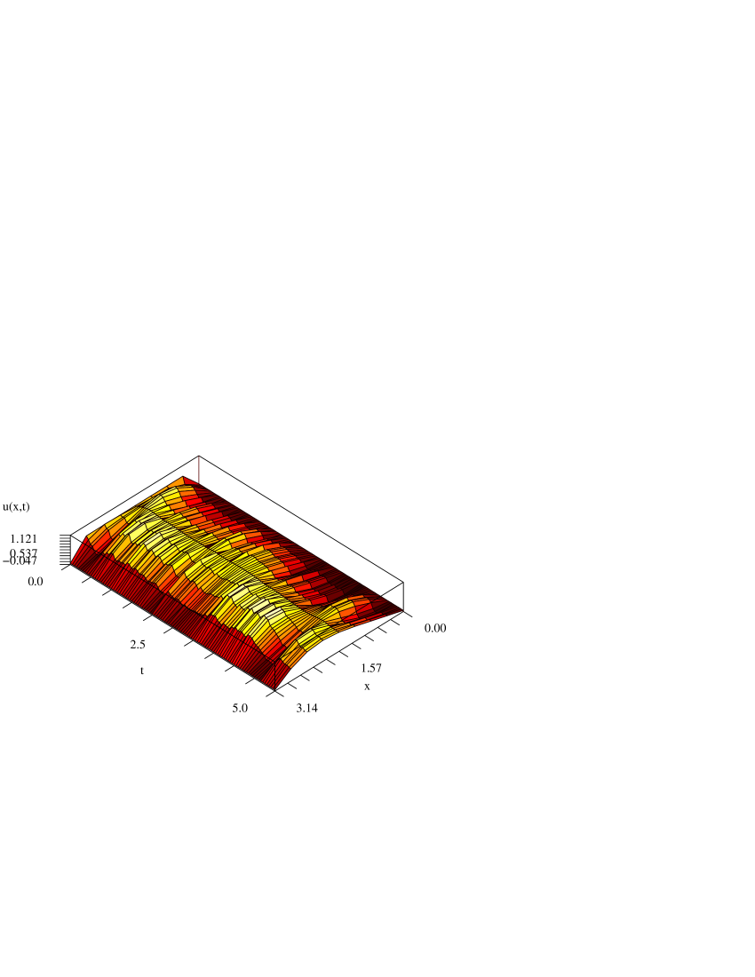
Figure 3: numerical solution of the spde (1) with relatively weak noise limited to just $\phi=\phi_{2}(t)\sin 2x$ showing convergence to a nonlinearly stabilised $\sin x$ mode that is perturbed by the noise. Parameters: $\sigma=0.5$ is small, $\gamma=-0.03$ to generate linear growth of the $\sin x$ mode, $\Delta t=0.05$ and $\Delta x=\pi/8$ .

An example numerical solution, Figure 3, displays that relatively weak noise only perturbs the deterministic dynamics. However, when the noise is large enough, then stochastic resonance restabilises the zero solution and the $\sin x$ mode decays as seen in Figure 4. The success of our approach is seen by it modelling this induced restabilisation.

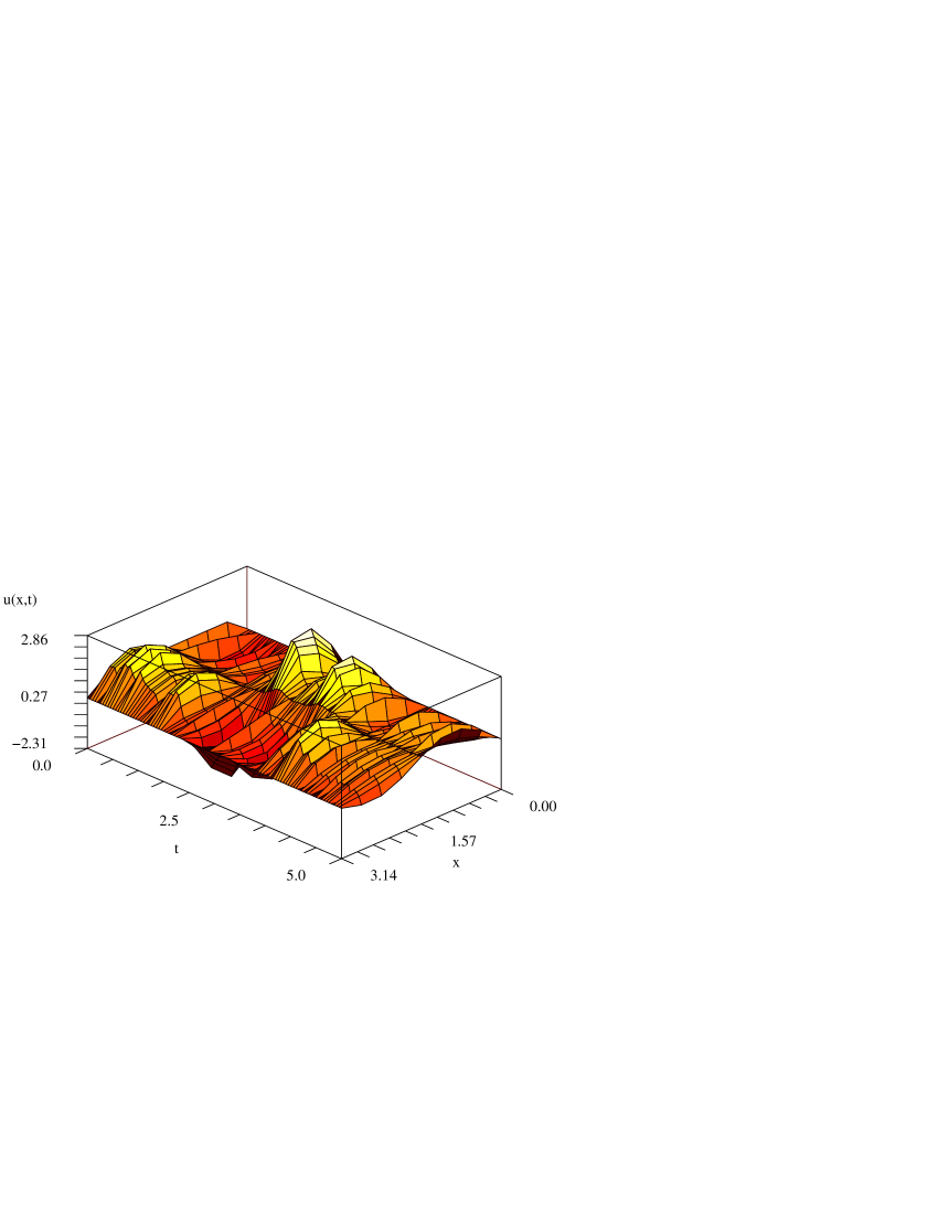
Figure 4: numerical solution of the spde (1) with strong noise limited to just $\phi=\phi_{2}(t)\sin 2x$ showing the $\sin x$ mode decays. Parameters: $\sigma=2$, $\gamma=-0.03$ to promote linear growth of the $\sin x$ mode, $\Delta t=0.05$ and $\Delta x=\pi/8$ .

For much of the analysis the requirement of white, delta correlated noise is irrelevant. Where it is relevant, we interpret the stochastic differential equations in the Stratonovich sense so that the rules of traditional calculus apply.

The centre manifold approach identifies that the long term dynamics of a spde such as (1) is parametrised by the amplitude $a(t)$ of the neutral mode $\sin x$ . Arnold et al. [1] investigated stochastic Hopf bifurcations this way, and the approach is equivalent to the slaving principle for sdes by Schoner and Haken [19]. Computer algebra [14] determines the solution field

$$u = a\sin x-{\textstyle\frac{1}{6}}a^{2}\sin 2x$$ (3)

$${}+\sigma{\cal H}_{2}(1-\gamma{\cal H}_{2})\phi_{2}\sin 2x-{\textstyle\frac{3}{2}}\sigma a{\cal H}_{3}{\cal H}_{2}(1-\gamma{\cal H}_{2})\phi_{2}\sin 3x$$

$${}+{\textstyle\frac{1}{3}}\sigma a^{2}{\cal H}_{4}(1+9{\cal H}_{3}){\cal H}_{2}\phi_{2}\sin 4x+{\cal O}\big{(}a^{3}+\gamma^{2},\sigma^{2}\big{)}\,,$$

in which the operator ${\cal H}_{m}$ denotes convolution with $\exp[-(m^{2}-1)t]$ . See in this formula the resolution of the subgrid structure arising through the interaction of the noise and the nonlinearity.

The model is the corresponding evolution equation for the amplitude:

$$\dot{a} = -\gamma a-{\textstyle\frac{1}{12}}a^{3}+\sigma a{\textstyle\frac{1}{2}}{\cal H}_{2}(1-\gamma{\cal H}_{2})\phi_{2}$$ (4)

$${}+\sigma a^{3}({\textstyle\frac{1}{64}}+{\textstyle\frac{1}{12}}{\cal H}_{2}-{\textstyle\frac{3}{4}}{\cal H}_{2}{\cal H}_{3}+{\textstyle\frac{1}{8}}{\cal H}_{3}){\cal H}_{2}\phi_{2}+{\cal O}\big{(}a^{4}+\gamma^{2},\sigma^{2}\big{)}\,.$$

This is an unduly messy model as it involves many convolutions over the rapid time scales we would like to “step over.” Straightforward analyses of forced systems often terminate at this point because of the tremendously involved form of the repeated convolutions that occur in higher order terms, especially higher order in the noise amplitude $\sigma$. However, some thought leads us to the drastic simplifications discussed next.

3 Use a normal form instead

Here we simplify the model by removing the convolutions from the evolution equation (4). This step was originally developed for sdes by Coullet et al. [6] and Sri Namachchivaya & Lin [13]. In computer algebra this is done in the equation for the updates to the field and the evolution:

$$\frac{\partial u^{\prime}}{\partial t}-\frac{\partial^{2}u^{\prime}}{\partial x^{2}}-u^{\prime}+{\dot{a}}^{\prime}\sin x=\mbox{residual}.$$

When the residual of the spde (1) contains a component of the form ${\cal H}_{m}\Phi\sin x$ , where $\Phi$ denotes some noise process, which previously we put into ${\dot{a}}^{\prime}$ to form (4), we instead recognise that

$$\frac{d}{dt}{\cal H}_{m}\Phi=-(m^{2}-1){\cal H}_{m}\Phi+\Phi\quad\mbox{thus}\quad{\cal H}_{m}\Phi=\frac{1}{m^{2}-1}\left[-\frac{d}{dt}{\cal H}_{m}\Phi+\Phi\right]\,,$$ (5)

and so the contribution in the residual is split into: a part that is integrated into the update $u^{\prime}$ for the subgrid field; and a part without the convolution for the update ${\dot{a}}^{\prime}$ for the evolution. Note that if the residual component has many convolutions, then this separation is applied recursively.

Computer algebra then deduces the normal form model

$$\dot{a}=-\gamma a-{\textstyle\frac{1}{12}}a^{3}+\sigma a({\textstyle\frac{1}{6}}-{\textstyle\frac{1}{18}}\gamma)\phi_{2}-\sigma^{2}a{\textstyle\frac{1}{44}}({\cal H}_{2}\phi_{2}-3{\cal H}_{3}{\cal H}_{2}\phi_{2})\phi_{2}+{\cal O}\big{(}a^{4}+\gamma^{2},\sigma^{3}\big{)}\,,$$ (6)

for the amplitude $a$ of the $\sin x$ mode, and now to quadratic terms in the noise. See that $a=0$ is always a fixed point of this sde. Numerical solutions of this model (6), see Figure 2, confirm that for the linearly unstable (deterministically) parameter $\gamma=-0.03$ large amounts of noise restabilise the zero solution.

4 Stochastic resonance affects deterministic terms

The noise $\phi_{2}(t)$ so far could have been any distributed forcing at all, random or deterministic. The analysis and the results are generally valid. We proceed to address the specific modelling when we restrict the noise $\phi_{2}(t)$ to be stochastic white noise in the Stratonovich sense.

Previously, the model was a strong model in that (6) could faithfully track given realisations of the original spde; however, now we derive the weak model (11) which maintains fidelity to solutions of the original spde, but we cannot know which realisation.

The relevant feature of the large time model (6) is the inescapable and undesirable appearance in the model of fast time convolutions in the quadratic noise term, namely ${\cal H}_{2}\phi_{2}=e^{-3t}\star\phi_{2}$ and ${\cal H}_{3}{\cal H}_{2}\phi_{2}=e^{-8t}\star e^{-3t}\star\phi_{2}$. These are undesirable because they require resolution of the fast time response of the system to these fast time dynamics in order to maintain fidelity with the original spde (1). However, maintaining fidelity with the full details of a white noise source is a pyrrhic victory when all we are interested in is the long term dynamics. Instead we should only be interested in those parts of the quadratic noise factors, $\phi_{2}{\cal H}_{2}\phi_{2}$ and $\phi_{2}{\cal H}_{3}{\cal H}_{2}\phi_{2}$, that over long time scales are firstly correlated with the other processes that appear and secondly independent of the other processes: these not only introduce factors in new independent noises into the model but also introduces a deterministic drift due to stochastic resonance [5, 7, e.g.].

The argument by Chao & Roberts [5, §4.1] asserts that we are interested in the long term statistics of the two quadratic noise processes $y_{1}$ and $y_{2}$ evolving according to

$$\dot{y}_{1}=z_{1}\phi_{2}\,,\quad\dot{y}_{2}=z_{2}\phi_{2}\,,\quad\dot{z}_{1}=-\beta_{1}z_{1}+\phi_{2}\,,\quad\dot{z}_{2}=-\beta_{2}z_{2}+z_{1}\,,$$ (7)

where here the decay rates $\beta_{1}=3$ and $\beta_{2}=8$ so that the convolutions of the noise $\phi_{2}$ are represented by the variables $z_{1}={\cal H}_{2}\phi_{2}$ and $z_{2}={\cal H}_{3}{\cal H}_{2}\phi_{2}$ . From the Fokker-Planck equation for (7) we have determined that large time solutions have a probability distribution

$$\mbox{{pdf}}\propto p(y_{1},y_{2},t)\exp\left[-(\beta_{1}+\beta_{2})z_{1}^{2}+2\beta_{2}(\beta_{1}+\beta_{2})z_{1}z_{2}-\beta_{2}(\beta_{1}+\beta_{2})^{2}z_{2}^{2}\right]\,,$$

where the relatively slowly varying $p$ evolves according to the approximate equation

$$\frac{\partial p}{\partial t}=-\mbox{$\frac{1}{2}$}\frac{\partial p}{\partial y_{1}}+D:\mbox{\boldmath$\nabla$}\mbox{\boldmath$\nabla$}p+{\cal O}\big{(}\mbox{\boldmath$\nabla$}^{3}p\big{)}$$ (8)

where the diffusion matrix

$$D=\left[\begin{array}[]{cc}\frac{1}{4\beta_{1}}&\frac{1}{4\beta_{1}(\beta_{1}+\beta_{2})}\\ \frac{1}{4\beta_{1}(\beta_{1}+\beta_{2})}&\frac{1}{4\beta_{1}\beta_{2}(\beta_{1}+\beta_{2})}\end{array}\right]\,.$$

Interpret (8) as a Fokker-Planck equation and see it corresponds to the sdes

$$\dot{y}_{1}=\mbox{$\frac{1}{2}$}+\frac{\psi_{1}(t)}{\sqrt{2\beta_{1}}}\quad\mbox{and}\quad\dot{y}_{2}=\frac{1}{\beta_{1}+\beta_{2}}\left(\frac{\psi_{1}(t)}{\sqrt{2\beta_{1}}}+\frac{\psi_{2}(t)}{\sqrt{2\beta_{2}}}\right)\,,$$ (9)

where $\psi_{i}(t)$ are new noises independent of $\phi_{2}$ over long time scales. Thus on long time scales, and substituting for the decay rates $\beta_{i}$, we should replace the quadratic noises by the following:

$$\phi_{2}{\cal H}_{2}\phi_{2}=\mbox{$\frac{1}{2}$}+\frac{\psi_{1}(t)}{\sqrt{6}}\quad\mbox{and}\quad\phi_{2}{\cal H}_{3}{\cal H}_{2}\phi_{2}=\frac{\psi_{1}(t)}{11\sqrt{6}}+\frac{\psi_{2}(t)}{44}\,.$$ (10)

Thus the normal form model (6) is transformed to

$$\dot{a}=-\left(\gamma+{\textstyle\frac{\sigma^{2}}{88}}\right)a-{\textstyle\frac{1}{12}}a^{3}+\sigma a({\textstyle\frac{1}{6}}-{\textstyle\frac{1}{18}}\gamma)\phi_{2}-\sigma^{2}a({\textstyle\frac{2}{121\sqrt{6}}}\psi_{1}-{\textstyle\frac{1}{1936}}\psi_{2})\,.$$

Combining the new noises into one effective new noise the model is a little more simply written

$$\dot{a}=-\left(\gamma+{\textstyle\frac{\sigma^{2}}{88}}\right)a-{\textstyle\frac{1}{12}}a^{3}+\sigma a({\textstyle\frac{1}{6}}-{\textstyle\frac{1}{18}}\gamma)\phi_{2}+\sigma^{2}a{\textstyle\frac{\sqrt{515}}{1936\sqrt{3}}}\psi\,,$$ (11)

for some white noise $\psi(t)$ independent of $\phi_{2}$ over long times. Although the nonlinearity induced stochastic resonance generates the effectively new multiplicative noise, $\propto\sigma^{2}a\psi$ , its most significant effect is the enhancement of the stability of the equilibrium $a=0$ through the $\sigma^{2}a/88$ term. The equilibrium is stable for parameters $\gamma>-\sigma^{2}/88$ which neatly explains the differences in the stability seen in Figure 2 because, compared to $\gamma=-0.030$, the thresholds for stability are $-0.003$ and $-0.045$ for small and large noise respectively.

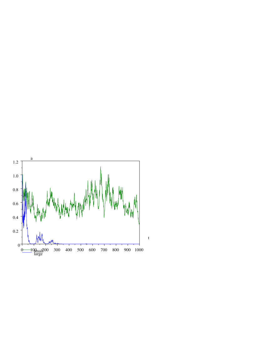
Figure 5: simulations of the long time model (11) for small, $\sigma=0.5$, and large, $\sigma=2$, noise over long times. Parameters: $\Delta t=1$, $\gamma=-0.03$ .

5 Conclusion

A big virtue of the model (11) is that we may accurately take large time steps as all the fast dynamics have been eliminated. Shown in Figure 5 are simulations over a long time for small and large noise again demonstrating the stochastic resonance induced stabilisation of the equilibrium $a=0$. These simulations are done for an order of magnitude longer times with a time step that is ten times larger than that we could use previously.

This approach to numerical modelling is viable and effective for stochastic partial differential equations. Much more development and theoretical support is needed.

References

- [1] L. Arnold, N. Sri Namachchivaya, and K. R. Schenk-Hoppé. Toward an understanding of stochastic Hopf bifurcation: a case study. Intl. J. Bifurcation & Chaos, 6:1947–1975, 1996.
- [2] Nils Berglund and Barbara Gentz. Geometric singular perturbation theory for stochastic differential equations. Technical report, [http://arXiv.org/abs/math.PR/0204008], 2003.
- [3] P. Boxler. A stochastic version of the centre manifold theorem. Probab. Th. Rel. Fields, 83:509–545, 1989.
- [4] P. Boxler. How to construct stochastic center manifolds on the level of vector fields. Lect. Notes in Maths, 1486:141–158, 1991.
- [5] Xu Chao and A. J. Roberts. On the low-dimensional modelling of stratonovich stochastic differential equations. Physica A, 225:62–80, 1996.
- [6] P. H. Coullet, C. Elphick, and E. Tirapegui. Normal form of a hopf bifurcation with noise. Physics Letts, 111A(6):277–282, 1985.
- [7] Francois Drolet and Jorge Vinals. Adiabatic reduction near a bifurcationn in stochastically modulated systems. Technical report, [http://arXiv.org/abs/patt-sol/9712001], 1997.
- [8] W. Grecksch and P. E. Kloeden. Time-discretised galerkin approximations of parabolic stochastics pdes. Bull. Austral Math. Soc., 54:79–85, 1996.
- [9] P. E. Kloeden and E. Platen. Numerical solution of stochastic differential equations, volume 23 of Applications of Mathematics. Springer-Verlag, 1992.
- [10] T. Mackenzie and A. J. Roberts. Holistic finite differences accurately model the dynamics of the Kuramoto-Sivashinsky equation. ANZIAM J., 42(E):C918–C935, 2000. [Online] http://anziamj.austms.org.au/V42/CTAC99/Mack.
- [11] T. MacKenzie and A. J. Roberts. Holistic discretisation of shear dispersion in a two-dimensional channel. In K. Burrage and Roger B. Sidje, editors, Proc. of 10th Computational Techniques and Applications Conference CTAC-2001, volume 44, pages C512–C530, March 2003. [Online] http://anziamj.austms.org.au/V44/CTAC2001/Mack [April 1, 2003].
- [12] A. Majda, I. Timofeyev, and E. Vanden-Eijnden. A priori tests of a stochastic mode reduction strategy. Physica D, 170:206 –252, 2002.
- [13] N. Sri Namachchivaya and Y. K. Lin. Method of stochastic normal forms. Int. J. Nonlinear Mechanics, 26:931–943, 1991.
- [14] A. J. Roberts. Low-dimensional modelling of dynamics via computer algebra. Computer Phys. Comm., 100:215–230, 1997.
- [15] A. J. Roberts. Holistic discretisation ensures fidelity to Burgers’ equation. Applied Numerical Modelling, 37:371–396, 2001.
- [16] A. J. Roberts. Holistic projection of initial conditions onto a finite difference approximation. Computer Physics Communications, 142:316–321, 2001.
- [17] A. J. Roberts. A holistic finite difference approach models linear dynamics consistently. Mathematics of Computation, 72:247–262, 2002.
- [18] A. J. Roberts. Derive boundary conditions for holistic discretisations of Burgers’ equation. In K. Burrage and Roger B. Sidje, editors, Proc. of 10th Computational Techniques and Applications Conference CTAC-2001, volume 44, pages C664–C686, March 2003. [Online] http://anziamj.austms.org.au/V44/CTAC2001/Robe [April 1, 2003].
- [19] G. Schöner and H. Haken. The slaving principle for stratonovich stochastic differential equations. Z. Phys. B—Condensed matter, 63:493–504, 1986.
- [20] M. J. Werner and P. D. Drummond. Robust algorithms for solving stochastic partial differential equations. J. Comput. Phys, 132:312–326, 1997.