Enumeration of totally positive Grassmann cells

Abstract.

Postnikov [7] has given a combinatorially explicit cell decomposition of the totally nonnegative part of a Grassmannian, denoted $Gr_{k,n}^{+}$, and showed that this set of cells is isomorphic as a graded poset to many other interesting graded posets. The main result of our work is an explicit generating function which enumerates the cells in $Gr_{k,n}^{+}$ according to their dimension. As a corollary, we give a new proof that the Euler characteristic of $Gr_{k,n}^{+}$ is $1$. Additionally, we use our result to produce a new $q$-analog of the Eulerian numbers, which interpolates between the Eulerian numbers, the Narayana numbers, and the binomial coefficients.

1. Introduction

The classical theory of total positivity concerns matrices in which all minors are nonnegative. While this theory was pioneered by Gantmacher, Krein, and Schoenberg in the 1930s, the past decade has seen a flurry of research in this area initiated by Lusztig [4, 5, 6]. Motivated by surprising connections he discovered between his theory of canonical bases for quantum groups and the theory of total positivity, Lusztig extended this subject by introducing the totally nonnegative variety $G_{\geq 0}$ in an arbitrary reductive group $G$ and the totally nonnegative part $B_{\geq 0}$ of a real flag variety $B$. A few years later, Fomin and Zelevinsky [2] advanced the understanding of $G_{\geq 0}$ by studying the decomposition of $G$ into double Bruhat cells, and Rietsch [8] proved Lusztig’s conjectural cell decomposition of $B_{\geq 0}$. Most recently, Postnikov [7] investigated the combinatorics of the totally nonnegative part of a Grassmannian $Gr_{k,n}^{+}$: he established a relationship between $Gr_{k,n}^{+}$ and planar oriented networks, producing a combinatorially explicit cell decomposition of $Gr_{k,n}^{+}$. In this paper we continue Postnikov’s study of the combinatorics of $Gr_{k,n}^{+}$: in particular, we enumerate the cells in the cell decomposition of $Gr_{k,n}^{+}$ according to their dimension.

The totally nonnegative part of the Grassmannian of $k$-dimensional subspaces in $\mathbb{R}^{n}$ is defined to be the quotient $Gr_{k,n}^{+}=\operatorname{GL}_{k}^{+}\backslash\operatorname{Mat}^{+}(k,n)$, where $\operatorname{Mat}^{+}(k,n)$ is the space of real $k\times n$-matrices of rank $k$ with nonnegative maximal minors and $\operatorname{GL}_{k}^{+}$ is the group of real matrices with positive determinant. If we specify which maximal minors are strictly positive and which are equal to zero, we obtain a cellular decomposition of $Gr_{k,n}^{+}$, as shown in [7]. We refer to the cells in this decomposition as totally positive cells. The set of totally positive cells naturally has the structure of a graded poset: we say that one cell covers another if the closure of the first cell contains the second, and the rank function is the dimension of each cell.

Lusztig [4] has proved that the totally nonnegative part of the (full) flag variety is contractible, which implies the same result for any partial flag variety. (We thank K. Rietsch for pointing this out to us.) The topology of the individual cells is not well understood, however. Postnikov [7] has conjectured that the closure of each cell in $Gr_{k,n}^{+}$ is homeomorphic to a closed ball.

In [7], Postnikov constructed many different combinatorial objects which are in one-to-one correspondence with the totally positive Grassmann cells (these objects thereby inherit the structure of a graded poset). Some of these objects include decorated permutations, -diagrams, positive oriented matroids, and move-equivalence classes of planar oriented networks. Because it is simple to compute the rank of a particular -diagram or decorated permutation, we will restrict our attention to these two classes of objects.

The main result of this paper is an explicit formula for the rank generating function $A_{k,n}(q)$ of $Gr_{k,n}^{+}$. Specifically, $A_{k,n}(q)$ is defined to be the polynomial in $q$ whose $q^{r}$ coefficient is the number of totally positive cells in $Gr_{k,n}^{+}$ which have dimension $r$. As a corollary of our main result, we give a new proof that the Euler characteristic of $Gr_{k,n}^{+}$ is $1$. Additionally, using our result and exploiting the connection between totally positive cells and permutations, we compute generating functions which enumerate (regular) permutations according to two statistics. This leads to a new $q$-analog of the Eulerian numbers that has many interesting combinatorial properties. For example, when we evaluate this $q$-analog at $q=1,0,$ and $-1$, we obtain the Eulerian numbers, the Narayana numbers, and the binomial coefficients. Finally, the connection with the Narayana numbers suggests a way of incorporating noncrossing partitions into a larger family of “crossing” partitions.

Let us fix some notation. Throughout this paper we use $[i]$ to denote the $q$-analog of $i$, that is, $[i]=1+q+\dots+q^{i-1}$. (We will sometimes use $[n]$ to refer to the set $\{1,\dots,n\}$, but the context should make our meaning clear.) Additionally, $[i]!:=\prod_{k=1}^{i}[k]$ and $\left[\begin{matrix}i\\ j\end{matrix}\right]:=\frac{[i]!}{[j]![i-j]!}$ are the $q$-analogs of $i!$ and ${i\choose j}$, respectively.

Acknowledgments: I thank Alex Postnikov for suggesting this problem to me, and for many helpful discussions. I am indebted to my advisor Richard Stanley for his invaluable advice and constant encouragement. And I thank Ira Gessel, Christian Krattenthaler, and Konni Rietsch for their very useful comments.

2. -Diagrams

A partition $\lambda=(\lambda_{1},\dots,\lambda_{k})$ is a weakly decreasing sequence of nonnegative numbers. For a partition $\lambda$, where $\sum\lambda_{i}=n$, the Young diagram $Y_{\lambda}$ of shape $\lambda$ is a left-justified diagram of $n$ boxes, with $\lambda_{i}$ boxes in the $i$th row. Figure 1 shows a Young diagram of shape $(4,2,1)$.

Figure 1. A Young diagram of shape $(4,2,1)$

Fix $k$ and $n$. Then a -diagram $(\lambda,D)_{k,n}$ is a partition $\lambda$ contained in a $k\times(n-k)$ rectangle (which we will denote by $(n-k)^{k}$), together with a filling $D:Y_{\lambda}\to\{0,1\}$ which has the -property: there is no $0$ which has a $1$ above it and a $1$ to its left. (Here, “above” means above and in the same column, and “to its left” means to the left and in the same row.) In Figure 2 we give an example of a -diagram.

Figure 2. A -diagram $(\lambda,D)_{k,n}$

We define the rank of $(\lambda,D)_{k,n}$ to be the number of $1$’s in the filling $D$. Postnikov proved that there is a one-to-one correspondence between -diagrams $(\lambda,D)$ contained in $(n-k)^{k}$, and totally positive cells in $Gr_{k,n}^{+}$, such that the dimension of a totally positive cell is equal to the rank of the corresponding -diagram. He proved this by providing a modified Gram-Schmidt algorithm $A$, which has the property that it maps a real $k\times n$ matrix of rank $k$ with nonnegative maximal minors to another matrix whose entries are all positive or $0$, which has the -property. In brief, the bijection between totally positive cells and -diagrams maps a matrix $M$ (representing some totally positive cell) to a -diagram whose $1$’s represent the positive entries of $A(M)$.

Because of this correspondence, in order to compute $A_{k,n}(q)$, we need to enumerate -diagrams contained in $(n-k)^{k}$ according to their number of $1$’s.

3. Decorated Permutations and the Cyclic Bruhat Order

The poset of decorated permutations (also called the cyclic Bruhat order) was introduced by Postnikov in [7]. A decorated permutation $\tilde{\pi}=(\pi,d)$ is a permutation $\pi$ in the symmetric group $S_{n}$ together with a coloring (decoration) $d$ of its fixed points $\pi(i)=i$ by two colors. Usually we refer to these two colors as “clockwise” and “counterclockwise,” for reasons which the next paragraph will make clear.

We represent a decorated permutation $\tilde{\pi}=(\pi,D)$, where $\pi\in S_{n}$, by its chord diagram, constructed as follows. Put $n$ equally spaced points around a circle, and label these points from $1$ to $n$ in clockwise order. If $\pi(i)=j$ then this is represented as a directed arrow, or chord, from $i$ to $j$. If $\pi(i)=i$ then we draw a chord from $i$ to $i$ (i.e. a loop), and orient it either clockwise or counterclockwise, according to $d$. We refer to the chord which begins at position $i$ as $\operatorname{Chord}(i)$, and we use $ij$ to denote the directed chord from $i$ to $j$. Also, if $i,j\in\{1,\dots,n\}$, we use $\operatorname{Arc}(i,j)$ to denote the set of points that we would encounter if we were to travel clockwise from $i$ to $j$, including $i$ and $j$.

For example, the decorated permutation $(3,1,5,4,8,6,7,2)$ (written in list notation) with the fixed points $4$, $6$, and $7$ colored in counterclockwise, clockwise, and counterclockwise, respectively, is represented by the chord diagram in Figure 3.

Figure 3. A chord diagram for a decorated permutation

The symmetric group $S_{n}$ acts on the permutations in $S_{n}$ by conjugation. This action naturally extends to an action of $S_{n}$ on decorated permutations, if we specify that the action of $S_{n}$ sends a clockwise (respectively, counterclockwise) fixed point to a clockwise (respectively, counterclockwise) fixed point.

We say that a pair of chords in a chord diagram forms a crossing if they intersect inside the circle or on its boundary.

Every crossing looks like Figure 4,

Figure 4. A crossing

where the point $A$ may coincide with the point $B$, and the point $C$ may coincide with the point $D$. A crossing is called a simple crossing if there are no other chords that go from $\operatorname{Arc}(C,A)$ to $\operatorname{Arc}(B,D)$. Say that two chords are crossing if they form a crossing.

Let us also say that a pair of chords in a chord diagram forms an alignment if they are not crossing and they are relatively located as in Figure 5.

Figure 5. An alignment

Here, again, the point $A$ may coincide with the point $B$, and the point $C$ may coincide with the point $D$. If $A$ coincides with $B$ then the chord from $A$ to $B$ should be a counterclockwise loop in order to be considered an alignment with $\operatorname{Chord}(C)$. (Imagine what would happen if we had a piece of string pointing from $A$ to $B$, and then we moved the point $B$ to $A$). And if $C$ coincides with $D$ then the chord from $C$ to $D$ should be a clockwise loop in order to be considered an alignment with $\operatorname{Chord}(A)$. As before, an alignment is a simple alignment if there are no other chords that go from $\operatorname{Arc}(C,A)$ to $\operatorname{Arc}(B,D)$. We say that two chords are aligned if they form an alignment.

We now define a partial order on the set of decorated permutations. For two decorated permutations $\pi_{1}$ and $\pi_{2}$ of the same size $n$, we say that $\pi_{1}$ covers $\pi_{2}$, and write $\pi_{1}\to\pi_{2}$, if the chord diagram of $\pi_{1}$ contains a pair of chords that forms a simple crossing and the chord diagram of $\pi_{2}$ is obtained by changing them to the pair of chords that forms a simple alignment (see Figure 6).

Figure 6. Covering relation

If the points $A$ and $B$ happen to coincide then the chord from $A$ to $B$ in the chord diagram of $\pi_{2}$ degenerates to a counterclockwise loop. And if the points $C$ and $D$ coincide then the chord from $C$ to $D$ in the chord diagram of $\pi_{2}$ becomes a clockwise loop. These degenerate situations are illustrated in Figure 7.

Figure 7. Degenerate covering relations

Let us define two statistics $A$ and $K$ on decorated permutations. For a decorated permutation $\pi$, the numbers $A(\pi)$ and $K(\pi)$ are given by

$$\begin{array}[]{l}A(\pi)=\#\{\textrm{pairs of chords forming an alignment}\},\\[7.22743pt] K(\pi)=\#\{i\mid\pi(i)>i\}+\#\{\textrm{counterclockwise loops}\}.\end{array}$$

In our previous example $\pi=(3,1,5,4,8,6,7,2)$ we have $A=11$ and $K=5$. The $11$ alignments in $\pi$ are $(13,66)$, $(21,35)$, $(21,58)$, $(21,44)$, $(21,77)$, $(35,44)$, $(35,66)$, $(44,66)$, $(58,77)$, $(66,77)$, $(66,82)$.

Lemma 3.1.

[7] If $\pi_{1}$ covers $\pi_{2}$ then $A(\pi_{1})=A(\pi_{2})-1$ and $K(\pi_{1})=K(\pi_{2})$.

Note that if $\pi_{1}$ covers $\pi_{2}$ then the number of crossings in $\pi_{1}$ is greater then the number of crossings in $\pi_{2}$. But the difference of these numbers is not always $1$.

Lemma 3.1 implies that the transitive closure of the covering relation “$\to$” has the structure of a partially ordered set and this partially ordered set decomposes into $n+1$ incomparable components. For $0\leq k\leq n$, we define the cyclic Bruhat order $\operatorname{CB}_{kn}$ as the set of all decorated permutations $\pi$ of size $n$ such that $K(\pi)=k$ with the partial order relation obtained by the transitive closure of the covering relation “$\to$”. By Lemma 3.1 the function $A$ is the corank function for the cyclic Bruhat order $\operatorname{CB}_{kn}$.

The definitions of the covering relation and of the statistic $A$ will not change if we rotate a chord diagram. The definition of $K$ depends on the order of the boundary points $1,\dots,n$, but it is not hard to see that the statistic $K$ is invariant under the cyclic shift $\textrm{conj}_{\sigma}$ for the long cycle $\sigma=(1,2,\dots,n)$. Thus the order $\operatorname{CB}_{kn}$ is invariant under the action of the cyclic group $\mathbb{Z}/n\mathbb{Z}$ on decorated permutations.

In [7], Postnikov proved that the number of totally positive cells in $Gr_{k,n}^{+}$ of dimension $r$ is equal to the number of decorated permutations in $\operatorname{CB}_{kn}$ of rank $r$. Thus, $A_{k,n}(1)$ is the cardinality of $\operatorname{CB}_{kn}$, and the coefficient of $q^{k(n-k)-\ell}$ in $A_{k,n}(q)$ is the number of decorated permutations in $\operatorname{CB}_{kn}$ with $\ell$ alignments.

4. The Rank Generating Function of $Gr_{k,n}^{+}$

Recall that the coefficient of $q^{r}$ in $A_{k,n}(q)$ is the number of cells of dimension $r$ in the cellular decomposition of $Gr_{k,n}^{+}$. In this section we use the -diagrams to find an explicit expression for $A_{k,n}(q)$. Additionally, we will find explicit expressions for the generating functions $A_{k}(q,x):=\sum_{n}A_{k,n}(q)x^{n}$ and $A(q,x,y):=\sum_{k\geq 1}\sum_{n}A_{k,n}(q)x^{n}y^{k}$. Our main theorem is the following:

Theorem 4.1.

$$A(q,x,y) =\frac{-y}{q(1-x)}+\sum_{i\geq 1}\frac{y^{i}(q^{2i+1}-y)}{q^{i^{2}+i+1}(q^{i}-q^{i}[i+1]x+[i]xy)}$$

$$A_{k}(q,x) =\sum_{i=0}^{k-1}(-1)^{i+k}\frac{x^{k-i-1}[i]^{k-i-1}}{q^{ki+i+1}(1-[i+1]x)^{k-i}}+\sum_{i=0}^{k}(-1)^{i+k}\frac{x^{k-i}[i]^{k-i}}{q^{ki}(1-[i+1]x)^{k-i+1}}$$

$$A_{k,n}(q) =q^{-k^{2}}\sum_{i=0}^{k-1}(-1)^{i}{n\choose i}(q^{ki}[k-i]^{i}[k-i+1]^{n-i}-q^{(k+1)i}[k-i-1]^{i}[k-i]^{n-i})$$

$$=\sum_{i=0}^{k-1}{n\choose i}q^{-(k-i)^{2}}([i-k]^{i}[k-i+1]^{n-i}-[i-k+1]^{i}[k-i]^{n-i}).$$

Note that it is not obvious that $A_{k,n}(q)$ is either polynomial or nonnegative.

Since the expressions for $A_{k}(q,x)$ and $A_{k,n}(q)$ follow easily from the formula for $A(q,x,y)$, we will concentrate on proving the formula for $A(q,x,y)$.

Fix a partition $\lambda=(\lambda_{1},\dots,\lambda_{k})$. Let $F_{\lambda}(q)$ be the polynomial in $q$ such that the coefficient of $q^{r}$ is the number of -fillings of the Young diagram $Y_{\lambda}$ which contain $r$ $1$’s. As Figure 8 illustrates, there is a simple recurrence for $F_{\lambda}(q)$.

Explicitly, any -filling of $\lambda$ is obtained in one of the following ways: adding a $1$ to the last row of a -filling of $(\lambda_{1},\lambda_{2},\dots,\lambda_{k-1},\lambda_{k}-1)$; adding a row containing $\lambda_{k}$ $0$’s to a -filling of $(\lambda_{1},\dots,\lambda_{k-1})$; or inserting an all-zero column after the $(\lambda_{k}-1)$st column of a -filling of $(\lambda_{1}-1,\lambda_{2}-1,\dots,\lambda_{k}-1)$. Note, however, that the second and third cases are not exclusive, so that our resulting recurrence must subtract off a term corresponding to their overlap.

Figure 8. Recurrence for $F_{\lambda}(q)$

Remark 4.2.

$$F_{\lambda}(q)=qF_{(\lambda_{1},\dots,\lambda_{k-1},\lambda_{k}-1)}(q)+F_{(\lambda_{1},\dots,\lambda_{k-1})}(q)+F_{(\lambda_{1}-1,\dots,\lambda_{k}-1)}(q)-F_{(\lambda_{1}-1,\dots,\lambda_{k-1}-1)}(q).$$

From the definition, or using the recurrence, it is easy to compute the first few formulas. Here are $F_{(\lambda_{1})}(q)$ and $F_{(\lambda_{1},\lambda_{2})}(q)$.

Proposition 4.3.

$$F_{(\lambda_{1})}(q) =[2]^{\lambda_{1}}$$

$$F_{(\lambda_{1},\lambda_{2})}(q) =-q^{-1}[2]^{\lambda_{1}}+q^{-1}[2]^{\lambda_{1}-\lambda_{2}+1}[3]^{\lambda_{2}}.$$

In general, we have the following formula.

Theorem 4.4.

Fix $\lambda=(\lambda_{1},\lambda_{2},\dots,\lambda_{k})$. Then

$$F_{\lambda}(q)=\sum_{i=1}^{k}\sum_{1=t_{1}<\dots<t_{i}\leq k}M(t_{1},\dots,t_{i}:k)[i+1]^{\lambda_{t_{i}}}\prod_{j=2}^{i}[j]^{\lambda_{t_{j-1}}-\lambda_{t_{j}}+1},$$

where $M(t_{1},\dots,t_{i}:k)=(-1)^{k+i}q^{-ik+\sum_{j=1}^{i}t_{j}}[i]^{k-t_{i}}\prod_{j=1}^{i-1}[j]^{t_{j+1}-t_{j}-1}.$

Before beginning the proof of the theorem, we state two lemmas which follow immediately from the formula for $M(t_{1},\dots,t_{i}:k)$.

Lemma 4.5.

$M(t_{1},\dots,t_{i}:k)=(-1)^{k-t_{i}}q^{-i(k-t_{i})}[i]^{k-t_{i}}M(t_{1},\dots,t_{i}:t_{i})$.

Lemma 4.6.

$M(t_{1},\dots,t_{i}:t_{i})=-[i-1]^{-1}M(t_{1},\dots,t_{i-1}:t_{i})$.

Proof.

To prove the theorem, we must show that the expression for $F_{\lambda}(q)$ holds for $\lambda=(\lambda_{1})$, and that it satisfies the recurrence of Remark 4.2. Also, we must show that $F_{(\lambda_{1},\lambda_{2},\dots,\lambda_{k})}(q)=F_{(\lambda_{1},\lambda_{2},\dots,\lambda_{k},0)}(q)$.

The formula $F_{(\lambda_{1})}(q)=[2]^{\lambda_{1}}$ clearly agrees with the expression in the theorem. To show that the recurrence is satisfied, we will fix $(t_{1},\dots,t_{i})$ where $1=t_{1}<\dots<t_{i}\leq k$, and calculate the coefficient of $[2]^{\lambda_{t_{1}}-\lambda_{t_{2}}+1}[3]^{\lambda_{t_{2}}-\lambda_{t_{3}}+1}\dots[i+1]^{\lambda_{t_{i}}}$ in each of the five terms of 4.2. We will then show that these coefficients satisfy the recurrence.

The coefficient in $F_{(\lambda_{1},\dots,\lambda_{k})}(q)$ is $M(t_{1},\dots,t_{i}:k)$.

The coefficient in $F_{(\lambda_{1},\lambda_{2},\dots,\lambda_{k}-1)}(q)$ is $M(t_{1},\dots,t_{i}:k)$ if $t_{i}<k$, because the term we are looking at together with its coefficient do not involve $\lambda_{k}$. The coefficient is $[i][i+1]^{-1}M(t_{1},\dots,t_{i}:k)$ if $t_{i}=k$.

The coefficient in $F_{(\lambda_{1},\lambda_{2},\dots,\lambda_{k-1})}(q)$ is $M(t_{1},\dots,t_{i}:k-1)$ if $t_{i}<k$, which is equal to $-q^{i}[i]^{-1}M(t_{1},\dots,t_{i}:k)$. But if $t_{i}=k$, no such term appears, so the coefficient is $0$.

The coefficient in $F_{(\lambda_{1}-1,\lambda_{2}-1,\dots,\lambda_{k}-1)}(q)$ is always $M(t_{1},\dots,t_{i}:k)[i+1]^{-1}$.

The coefficient in $F_{(\lambda_{1}-1,\lambda_{2}-1,\dots,\lambda_{k-1}-1)}(q)$ is $-q^{i}[i]^{-1}[i+1]^{-1}M(t_{1},\dots,t_{i}:k)$ if $t_{i}<k$, and $0$ if $t_{i}=k$.

Let us abbreviate $M(t_{1},\dots,t_{i}:k)$ by $M$. We need to show that the coefficients we have just calculated satisfy the recurrence of Remark 4.2. For $t_{i}<k$, this amounts to showing that $M=qM-q^{i}[i]^{-1}M+M[i+1]^{-1}+q^{i}[i]^{-1}[i+1]^{-1}M$. And for $t_{i}=k$, we must show that $M=q[i][i+1]^{-1}M+M[i+1]^{-1}$. Both of these are easily seen to be true. Thus, we have shown that our expression for $F_{\lambda}(q)$ satisfies Remark 4.2.

Now we will show that $F_{(\lambda_{1},\lambda_{2},\dots,\lambda_{k-1},0)}(q)=F_{(\lambda_{1},\lambda_{2},\dots,\lambda_{k-1})}(q)$. It is sufficient to show that the coefficient of $[2]^{\lambda_{t_{1}}-\lambda_{t_{2}}+1}[3]^{\lambda_{t_{2}}-\lambda_{t_{3}}+1}\dots[i+1]^{\lambda_{t_{i}}}$ in $F_{(\lambda_{1},\dots,\lambda_{k})}(q)$, plus $[i+1]$ times the coefficient of $[2]^{\lambda_{t_{1}}-\lambda_{t_{2}}+1}[3]^{\lambda_{t_{2}}-\lambda_{t_{3}}+1}\dots[i+1]^{\lambda_{t_{i}}-\lambda_{k}+1}[i+2]^{\lambda_{k}}$ in $F_{(\lambda_{1},\dots,\lambda_{k})}(q)$, is equal to the coefficient of $[2]^{\lambda_{t_{1}}-\lambda_{t_{2}}+1}\dots[i+1]^{\lambda_{t_{i}}}$ in $F_{(\lambda_{1},\dots,\lambda_{k-1})}(q)$.

In other words, we need

$$M(t_{1},\dots,t_{i}:k-1)=M(t_{1},\dots,t_{i}:k)+M(t_{1},\dots,t_{i},k:k)[i+1].$$

From the formula for $M$, we have $M(t_{1},\dots,t_{i}:k-1)=-q^{i}[i]^{-1}M(t_{1},\dots,t_{i}:k)$. And from Lemma 4.6, $M(t_{1},\dots,t_{i},k:k)=-[i]^{-1}M(t_{1},\dots,t_{i}:k)$. The proof follows. ∎

Recall that $A_{k}(q,x)$ is the polynomial in $q$ and $x$ such that $[q^{r}x^{n}]A_{k}(q,x)$ is equal to the number of totally positive cells of dimension $r$ in $Gr_{k,n}^{+}$. This is equal to the number of -diagrams $(\lambda,D)_{k,n}$ of rank $r$. We can compute these numbers by using Theorem 4.4.

Corollary 4.7.

$$A_{k}(q,x)=\sum_{i=1}^{k}\sum_{1=t_{1}<\dots<t_{i+1}=k+1}\frac{(-1)^{k+i}q^{-ik+\sum_{j=1}^{i}t_{j}}x^{k}}{(1-x)}\prod_{j=1}^{i}\left(\frac{[j]}{1-[j+1]x}\right)^{t_{j+1}-t_{j}}.$$

To compute $A_{k}(q,x)$, we must sum $F_{(\lambda_{1},\dots,\lambda_{k})}(q)x^{n}$, as $\lambda$ varies over all partitions which fit into a $k\times(n-k)$ rectangle. To do this, we use the following simple lemmas, the second of which follows immediately from the first.

Lemma 4.8.

$$\sum_{\lambda_{1}=0}^{\infty}\sum_{\lambda_{2}=0}^{\lambda_{1}}\dots\sum_{\lambda_{d}=0}^{\lambda_{d-1}}x_{1}^{\lambda_{1}}x_{2}^{\lambda_{2}}\dots x_{d}^{\lambda_{d}}=\frac{1}{(1-x_{1})(1-x_{1}x_{2})\dots(1-x_{1}x_{2}\dots x_{d})}.$$

Lemma 4.9.

Fix a set of positive integers $t_{1}<t_{2}<\dots<t_{d}<n+1$. Then

$$\sum_{n=0}^{\infty}\sum_{\lambda_{1}=0}^{n}\sum_{\lambda_{2}=0}^{\lambda_{1}}\dots\sum_{\lambda_{d}=0}^{\lambda_{d-1}}[2]^{\lambda_{t_{1}}-\lambda_{t_{2}}}\dots[d]^{\lambda_{t_{d-1}}-\lambda_{t_{d}}}[d+1]^{\lambda_{t_{d}}}x^{n}$$

is equal to

$$\frac{1}{(1-x)(1-[2]x)^{t_{2}-t_{1}}\dots(1-[d]x)^{t_{d}-t_{d-1}}(1-[d+1]x)^{n+1-t_{d}}}.$$

Proof.

For the proof of the corollary, apply Theorem 4.4 and Lemma 4.9 to the fact that

$$A_{k}(q,x)=\sum_{m=0}^{\infty}\sum_{\lambda_{1}=0}^{m}\sum_{\lambda_{2}=0}^{\lambda_{1}}\dots\sum_{\lambda_{k}=0}^{\lambda_{k-1}}F_{(\lambda_{1},\dots,\lambda_{k})}(q)x^{m}.$$

∎

Corollary 4.10.

The Euler characteristic of the totally non-negative part of the Grassmannian $Gr_{k,n}^{+}$ is $1$.

Proof.

Recall that the Euler characteristic of a cell complex is defined to be $\sum_{i}(-1)^{i}f_{i}$, where $f_{i}$ is the number of cells of dimension $i$. So if we set $q=-1$ in Corollary 4.7, we will obtain a polynomial in $x$ such that the coefficient of $x^{n}$ is the Euler characteristic of $Gr_{k,n}^{+}$. Notice that $[i]$ is equal to $0$ if $i$ is even, and $1$ if $i$ is odd. So all terms of $A_{k}(-1,x)$ vanish except the term for $i=1$, which becomes $\frac{x^{k}}{1-x}=x^{k}+x^{k+1}+x^{k+2}+\dots$. ∎

Note that this corollary also follows from Lusztig’s result that the totally nonnegative part of a real flag variety is contractible.

Now our goal will be to simplify our expressions. To do so, it is helpful to work with the “master” generating function $A(q,x,y):=\sum_{k\geq 1}A_{k}(q,x)y^{k}$. As a first step, we compute the following expression for $A(q,x,y)$:

Proposition 4.11.

$$A(q,x,y)=\sum_{i=1}^{\infty}q^{i}[i]!x^{i}y^{i}\prod_{j=0}^{i}\frac{1}{q^{j}-q^{j}[j+1]x+[j]xy}.$$

Note that $\frac{1}{q^{j}-q^{j}[j+1]x+[j]xy}$ is not a well-defined formal power series because it is not clear how to expand it. In this paper, for reasons which will become clear in the following proof, we shall always use $\frac{1}{q^{j}-q^{j}[j+1]x+[j]xy}$ as shorthand for the formal power series whose expansion is implied by the expression

$$\frac{1}{q^{j}(1-[j+1]x)(1-\frac{q^{-j}[j]y}{1-[j+1]x})}.$$

See [9, Example 6.3.4] for remarks on the subtleties of such power series.

Proof.

From Corollary 4.7, we know that $A_{k}(q,x)$ is equal to

$$\frac{(-x)^{k}}{1-x}\sum_{i=1}^{k}\sum_{1=t_{1}<\dots<t_{i+1}=k+1}(-1)^{i}q^{-ik+\sum_{j=1}^{i}t_{j}}\prod_{j=1}^{i}\left(\frac{[j]}{1-[j+1]x}\right)^{t_{j+1}-t_{j}}.$$

If we make the substitution $\alpha_{j}=t_{j+1}-t_{j}$, we then get

$$A_{k}(q,x)=\frac{(-x)^{k}}{1-x}\sum_{i=1}^{k}(-1)^{i}q^{i}\sum_{\begin{subarray}{c}\alpha_{j}\geq 1\\ \alpha_{1}+\dots+\alpha_{i}=k\end{subarray}}\prod_{j=1}^{i}\left(\frac{[j]}{q^{j}(1-[j+1]x)}\right)^{\alpha_{j}}.$$

Now let $f_{j}(p)=(\frac{[j]}{q^{j}(1-[j+1]x)})^{p}$. For future use, define $F_{j}(y):=\sum_{p\geq 1}f_{j}(p)y^{p},$ which is equal to $\frac{[j]y}{q^{j}-q^{j}[j+1]x-[j]y}$. We get

$$A_{k}(q,x)=\frac{(-x)^{k}}{1-x}\sum_{i=1}^{k}(-1)^{i}q^{i}\sum_{\begin{subarray}{c}\alpha_{j}\geq 1\\ \alpha_{1}+\dots+\alpha_{i}=k\end{subarray}}\prod_{j=1}^{i}f_{j}(\alpha_{j}),$$

and we can now easily compute $A(q,x,y):=\sum_{k\geq 1}A_{k}(q,x)y^{k}$.

$$A(q,x,y) =\frac{1}{1-x}\sum_{k\geq 1}(-x)^{k}\sum_{i=1}^{k}(-1)^{i}q^{i}\sum_{\begin{subarray}{c}\alpha_{j}\geq 1\\ \alpha_{1}+\dots+\alpha_{i}=k\end{subarray}}\prod_{j=1}^{i}f_{j}(\alpha_{j})y^{\alpha_{j}}$$

$$=\frac{1}{1-x}\sum_{i=1}^{\infty}\sum_{k\geq i}\sum_{\begin{subarray}{c}\alpha_{j}\geq 1\\ \alpha_{1}+\dots+\alpha_{i}=k\end{subarray}}(-x)^{k}(-1)^{i}q^{i}\prod_{j=1}^{i}f_{j}(\alpha_{j})y^{\alpha_{j}}.$$

Actually, we can replace $k\geq i$ above with $k\geq 0$, since if $k<i$ there will be no set of $\alpha_{j}$ satisfying the conditions of the third sum. So we have

$$A(q,x,y) =\frac{1}{1-x}\sum_{i=1}^{\infty}\sum_{k\geq 0}\sum_{\begin{subarray}{c}\alpha_{j}\geq 1\\ \alpha_{1}+\dots+\alpha_{i}=k\end{subarray}}(-x)^{k}(-1)^{i}q^{i}\prod_{j=1}^{i}f_{j}(\alpha_{j})y^{\alpha_{j}}$$

$$=\frac{1}{1-x}\sum_{i=1}^{\infty}(-1)^{i}q^{i}\sum_{k\geq 0}\sum_{\begin{subarray}{c}\alpha_{j}\geq 1\\ \alpha_{1}+\dots+\alpha_{i}=k\end{subarray}}\prod_{j=1}^{i}f_{j}(\alpha_{j})(-xy)^{\alpha_{j}}.$$

Using the definition of $F_{j}$, we get

$$A(q,x,y) =\frac{1}{1-x}\sum_{i=1}^{\infty}(-1)^{i}q^{i}\prod_{j=1}^{i}F_{j}(-xy)$$

$$=\frac{1}{1-x}\sum_{i=1}^{\infty}(-1)^{i}q^{i}\prod_{j=1}^{i}\frac{-[j]xy}{q^{j}-q^{j}[j+1]x+[j]xy}$$

$$=\frac{1}{1-x}\sum_{i=1}^{\infty}q^{i}[i]!x^{i}y^{i}\prod_{j=1}^{i}\frac{1}{q^{j}-q^{j}[j+1]x+[j]xy}$$

$$=\frac{1}{1-x}\sum_{i=1}^{\infty}q^{i}[i]!x^{i}y^{i}\prod_{j=1}^{i}\frac{1}{q^{j}-q^{j}[j+1]x+[j]xy}$$

$$=\sum_{i=1}^{\infty}q^{i}[i]!x^{i}y^{i}\prod_{j=0}^{i}\frac{1}{q^{j}-q^{j}[j+1]x+[j]xy}.$$

∎

Now we will prove the following identity. This identity combined with Proposition 4.11 will complete the proof of Theorem 4.1.

Theorem 4.12.

$$\sum_{i=1}^{\infty}q^{i}[i]!x^{i}y^{i}\prod_{j=0}^{i}\frac{1}{q^{j}-q^{j}[j+1]x+[j]xy}=\frac{-y}{q(1-x)}+\sum_{i\geq 1}\frac{q^{-i^{2}-i-1}y^{i}(q^{2i+1}-y)}{q^{i}-q^{i}[i+1]x+[i]xy}$$

Proof.

Observe that the expression on the right-hand side can be thought of as a partial fraction expansion in terms of $x$, since all denominators are distinct, and the numerators are free of $x$. Also note that the $i$-summand of the left-hand side should be easy to express in partial fractions with respect to $x$, since all factors of the denominator are distinct and the $x$-degree of the numerator is smaller than the $x$-degree of the denominator.

Thus, our strategy will be to put the left-hand side into partial fractions with respect to $x$, and then show that this agrees with the right-hand side.

To this end, define $\beta_{i}(j)$ by the equation

$$\frac{x^{i}}{\prod_{j=0}^{i}{q^{j}-q^{j}[j+1]x+[j]xy}}=\sum_{j=0}^{i}\frac{\beta_{i}(j)}{q^{j}-q^{j}[j+1]x+[j]xy}.$$

Clearing denominators, we obtain

(1) $$x^{i}=\sum_{j=0}^{i}\beta_{i}(j)\prod_{\begin{subarray}{c}r=0\\ r\neq j\end{subarray}}^{i}(q^{r}-q^{r}[r+1]x+[r]xy).$$

Fix $j$. Notice that $(q^{j}-q^{j}[j+1]x+[j]xy)$ vanishes when $x=\frac{q^{j}}{q^{j}[j+1]-[j]y}$, so substitute $x=\frac{q^{j}}{q^{j}[j+1]-[j]y}$ into (1). We get

$$\frac{q^{ij}}{(q^{j}[j+1]-[j]y)^{i}}=\beta_{i}(j)\prod_{\begin{subarray}{c}r=0\\ r\neq j\end{subarray}}^{i}\frac{q^{r}(q^{j}[j+1]-[j]y)+q^{j}([r]y-q^{r}[r+1])}{q^{j}[j+1]-[j]y}.$$

Solving for $\beta_{i}(j)$ and simplifying, we arrive at

$$\beta_{i}(j)=\frac{(-1)^{i+j}q^{\frac{j^{2}+3j-i^{2}-3i-2ij}{2}}}{\displaystyle{[j]![i-j]!\prod_{\begin{subarray}{c}r=0\\ r\neq j\end{subarray}}^{i}(1-q^{-r-j-1}y)}}.$$

Thus the partial fraction expansion with respect to $x$ of the left-hand side of Theorem 4.12 is

$$\sum_{i=1}^{\infty}\sum_{j=0}^{i}\frac{\beta_{i}(j)q^{i}[i]!y^{i}}{q^{j}-q^{j}[j+1]x+[j]xy},$$

which is equal to

(2) $$\sum_{j=0}^{\infty}\frac{{\displaystyle(-1)^{j}q^{\frac{j^{2}+3j}{2}}\sum_{\begin{subarray}{c}i\geq j\\ i\neq 0\end{subarray}}\left[\begin{matrix}i\\ j\end{matrix}\right]q^{-{i+1\choose 2}-ij}(-y)^{i}\prod_{\begin{subarray}{c}r=0\\ r\neq j\end{subarray}}^{i}(1-q^{-r-j-1}y)^{-1}}}{q^{j}-q^{j}[j+1]x+[j]xy}.$$

Now it remains to show that the numerator of $(q^{j}-q^{j}[j+1]x+[j]xy)$ in (2) is equal to the numerator of $(q^{j}-q^{j}[j+1]x+[j]xy)$ in the right-hand side of Theorem 4.12. For $j=0$, we must show that

(3) $$(1-\frac{y}{q})\sum_{i\geq 1}(-1)^{i}q^{-{i+1\choose 2}}y^{i}\prod_{r=0}^{i}(1-q^{-r-1}y)^{-1}=\frac{-y}{q}.$$

And for $j>0$, we must show that

(4) $$(-1)^{j}q^{\frac{3j^{2}+j}{2}}y^{-j}\sum_{i\geq j}\left[\begin{matrix}i\\ j\end{matrix}\right]q^{-{i+1\choose 2}-ij}(-y)^{i}\prod_{r=0}^{i}(1-q^{-r-j-1}y)^{-1}=1.$$

If we make the substitution $q\to q^{-1}$ and $r\to r-1$ into (3) and then add the $i=0$ term to both sides, we obtain

(5) $$\sum_{i\geq 0}(-1)^{i}y^{i}q^{i+1\choose 2}\prod_{r=1}^{i+1}\frac{1}{1-q^{r}y}=1.$$

And if we make the same substitution into (4), we get

(6) $$(-1)^{j}q^{-{j+1\choose 2}}y^{-j}\sum_{i\geq j}(-1)^{i}q^{{i+1\choose 2}}\left[\begin{matrix}i\\ j\end{matrix}\right]y^{i}\prod_{r=1}^{i+1}\frac{1}{1-q^{r+j}y}=1.$$

Since (5) is a special case of (6), it suffices to prove (6). We will prove this as a separate lemma below; modulo this lemma, we are done. ∎

Lemma 4.13.

$$(-1)^{j}q^{-{j+1\choose 2}}y^{-j}\sum_{i\geq j}(-1)^{i}q^{i+1\choose 2}\left[\begin{matrix}i\\ j\end{matrix}\right]y^{i}\prod_{r=1}^{i+1}\frac{1}{1-q^{r+j}y}=1.$$

Proof.

Christian Krattenthaler has pointed out to us that this lemma is actually a special case of the ${}_{1}\phi_{1}$ summation described in Appendix II.5 of [3]. Here, we give two additional proofs of this lemma. The first method is to show that the infinite sum actually telescopes (we thank Ira Gessel for suggesting this to us). The second method is to interpret the lemma as a statement about partitions, and to prove it combinatorially.

Let us sketch the first method. We use induction to show that

$$(-1)^{j}q^{-{j+1\choose 2}}y^{-j}\sum_{i=j}^{m-1}(-1)^{i}q^{{i+1\choose 2}}\left[\begin{matrix}i\\ j\end{matrix}\right]y^{i}\prod_{r=1}^{i+1}\frac{1}{1-q^{r+j}y}$$

is equal to

$$1+\frac{{\displaystyle(-1)^{m-1}q^{jm+{m+1\choose 2}}y^{m}\sum_{p=0}^{j}(-1)^{p}\left[\begin{matrix}m\\ p\end{matrix}\right]q^{{p\choose 2}-pj-pm}y^{-p}}}{\prod_{r=1}^{m}(1-q^{r+j}y)}.$$

Then we take the limit as $m$ goes to $\infty$, obtaining the statement of the lemma.

Now let us give a combinatorial proof of the lemma. For clarity, we prove the $j=0$ case in detail and then explain how to generalize this proof.

First we claim that $(-1)^{i}y^{i}q^{i+1\choose 2}\prod_{r=1}^{i+1}\frac{1}{1-q^{r}y}$ is a generating function for partitions $\lambda$ with $i+1$ parts, all distinct, where the smallest part may be zero. In this formal power series, the coefficient of $y^{m}q^{n}$ is equal to the number of such partitions with $m$ columns and $n$ total boxes. The generating function is multiplied by $1$ or $-1$, according to the parity of the number of rows (including zero).

To prove the claim, note that each term of $\prod_{r=1}^{i+1}\frac{1}{1-q^{r}y}$ corresponds to a (normal) partition where rows have lengths between $1$ and $i+1$, inclusive. The exponent of $y$ enumerates the number of rows and the exponent of $q$ enumerates the number of boxes. Now take the transpose of this partition, so that it is a partition with exactly $i+1$ rows (possibly zero). Now the exponent of $y$ is the length of the longest row. Add $i,i-1,\dots,1$ and $0$ boxes to the first, second, … , and $(i+1)$st rows, respectively. Finally we have a partition with $i+1$ parts, all distinct, where the smallest part may be zero. Since we’ve added a total of ${i+1\choose 2}$ boxes to the original partition, the generating function for this type of partition is $q^{i+1\choose 2}y^{i}\prod_{r=1}^{i+1}\frac{1}{1-q^{r}y}$. Figure 9 illustrates the steps in this paragraph. In the figure, the rows and columns of the partitions are indicated by solid and dashed lines, respectively.

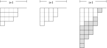
Figure 9. A Combinatorial interpretation for $y^{i}q^{i+1\choose 2}\prod_{r=1}^{i+1}\frac{1}{1-q^{r}y}$

Now we need to find an involution $\phi$ which explains why all of the terms on the left-hand side of (5) cancel out, except for the $1$. This involution is very simple: if $(\lambda_{1},\dots,\lambda_{k})$ is a partition such that $\lambda_{k}\neq 0$, then $\phi(\lambda_{1},\dots,\lambda_{k})=(\lambda_{1},\dots,\lambda_{k},0)$. And if $\lambda_{k}=0$, then $\phi(\lambda_{1},\dots,\lambda_{k})=(\lambda_{1},\dots,\lambda_{k-1})$. Clearly both $(\lambda_{1},\dots,\lambda_{k})$ and $\phi(\lambda_{1},\dots,\lambda_{k})$ contribute the same powers of $y$ and $q$ to the generating function; the only difference is the sign. Only the $0$ partition has no partner under the involution, so all terms cancel except for $1$.

For the proof of the general case, we will show that

(7) $$q^{i+1\choose 2}\left[\begin{matrix}i\\ j\end{matrix}\right]y^{i-j}\prod_{r=1}^{i+1}\frac{1}{1-q^{r+j}y}$$

is a generating function for certain pairs of partitions, $(\lambda,\hat{\lambda})$. First, note that $\prod_{r=1}^{i+1}\frac{1}{1-q^{r+j}y}$ is a generating function for partitions with rows of lengths $j+1$ through $i+j+1$, inclusive. It is well-known that $\left[\begin{matrix}i\\ j\end{matrix}\right]$ is a polynomial in $q$ whose $q^{r}$ coefficient is the number of partitions of $r$ which fit inside a $j\times(i-j)$ rectangle. To account for the $\left[\begin{matrix}i\\ j\end{matrix}\right]$ term in (7), let us take a partition which fits inside a $j\times(i-j)$ rectangle, and place it underneath a partition with rows of lengths $j+1$ through $i+j+1$, giving us a partition with row lengths between $0$ and $i+j+1$, inclusive. We consider this partition to have exactly $i+j+1$ columns, possibly zero. Finally, to account for the $q^{i+1\choose 2}$ term in (7) let us add $0,1,\dots,i$ boxes to the last $i+1$ columns of our partition, so that that the last $i+1$ columns have distinct lengths (possibly zero). We now view the boxes in the first $j$ columns of our figure to comprise one partition $\lambda$, and the boxes in the last $i+1$ columns of our figure to comprise the transpose of a second partition $\hat{\lambda}$. Let $\hat{\lambda}_{1}$ denote the length of the first row of $\hat{\lambda}$, and let $r_{j}(\lambda)$ denote the number of rows of $\lambda$ which have length $j$. Then the pair $(\lambda,\hat{\lambda})$ satisfies the following conditions: $\lambda$ has rows with lengths between $0$ and $j$, inclusive; $\hat{\lambda}$ has exactly $i+1$ rows, all distinct, where the smallest row can have length $0$; and $r_{j}(\lambda)+i-j=\hat{\lambda}_{1}$. (See Figure 10 for an illustration of $(\lambda,\hat{\lambda})$.) The term in (7) that corresponds to this pair of partitions is $q^{|\lambda|+|\hat{\lambda}|}y^{\operatorname{numparts}(\lambda)}$.

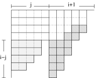
Figure 10. $(\lambda,\hat{\lambda})$, where $\lambda=(5,5,5,5,4,4,3,2,0)$ and $\hat{\lambda}=(9,8,6,4,3,0)$

Our involution $\phi$ is a simple generalization of the involution we used before. This time, $\phi$ fixes $\lambda$, and either adds or subtracts a trailing zero to $\hat{\lambda}$.

∎

This completes the proof of Theorem 4.1.

In Table 1, we have listed some of the values of $A_{k,n}(q)$ for small $k$ and $n$. It is easy to see from the definition of -diagrams that $A_{k,n}(q)=A_{n-k,n}(q)$: one can reflect a -diagram $(\lambda,D)_{k,n}$ of rank $r$ over the main diagonal to get another -diagram $(\lambda^{\prime},D^{\prime})_{n-k,n}$ of rank $r$. Alternatively, one should be able to prove the claim directly from the expression in Theorem 4.1, using some $q$-analog of Abel’s identity.

$A_{1,1}(q)$	$1$
$A_{1,2}(q)$	$q+2$
$A_{1,3}(q)$	$q^{2}+3q+3$
$A_{1,4}(q)$	$q^{3}+4q^{2}+6q+4$
$A_{2,4}(q)$	$q^{4}+4q^{3}+10q^{2}+12q+6$
$A_{2,5}(q)$	$q^{6}+5q^{5}+15q^{4}+30q^{3}+40q^{2}+30q+10$
$A_{2,6}(q)$	$q^{8}+6q^{7}+21q^{6}+50q^{5}+90q^{4}+120q^{3}+110q^{2}+60q+15$
$A_{3,6}(q)$	$q^{9}+6q^{8}+21q^{7}+56q^{6}+114q^{5}+180q^{4}+215q^{3}+180q^{2}+90q+20$
$A_{3,7}(q)$	$q^{12}+7q^{11}+28q^{10}+84q^{9}+203q^{8}+406q^{7}+679q^{6}+938q^{5}+1050q^{4}+910q^{3}+560q^{2}+210q+35$

Table 1. $A_{k,n}(q)$

Note that it is possible to see directly from the definition that $Gr_{1,n}^{+}$ is just some deformation of a simplex with $n$ vertices. This explains the simple form of $A_{1,n}(q)$.

5. A New $q$-Analog of the Eulerian Numbers

If $\pi\in S_{n}$, we say that $\pi$ has a weak excedence at position $i$ if $\pi(i)\geq i$. The Eulerian number $E_{k,n}$ is the number of permutations in $S_{n}$ which have $k$ weak excedences. (One can define the Eulerian numbers in terms of other statistics, such as descent, but this will not concern us here.)

Now that we have computed the rank generating function for $\operatorname{CB}_{kn}^{+}$ (which is the rank generating function for the poset of decorated permutations), we can use this result to enumerate (regular) permutations according to two statistics: weak excedences and alignments. This gives us a new $q$-analog of the Eulerian numbers.

Recall that the statistic $K$ on decorated permutations was defined as

$$K(\pi)=\#\{i\mid\pi(i)>i\}+\#\{\textrm{counterclockwise loops}\}.$$

Note that $K$ is related to the notion of weak excedence in permutations. In fact, we can extend the definition of weak excedence to decorated permutations by saying that a decorated permutation has a weak excedence in position $i$, if $\pi(i)>i$, or if $\pi(i)=i$ and $d(i)$ is counterclockwise. This makes sense, since the limit of a chord from $1$ to $2$ as $1$ approaches $2$, is a counterclockwise loop. Then $K(\pi)$ is the number of weak excedences in $\pi$.

We will call a decorated permutation regular if all of its fixed points are oriented counterclockwise. Thus, a fixed point of a regular permutation will always be a weak excedence, as it should be. Recall that the Eulerian number $E_{k,n}$ is the number of permutations of $[n]$ with $k$ weak excedences. Earlier, we saw that the coefficient of $q^{k(n-k)-\ell}$ in $A_{k,n}(q)$ is the number of decorated permutations in $\operatorname{CB}_{kn}$ with $\ell$ alignments. By analogy, let $E_{k,n}(q)$ be the polynomial in $q$ whose coefficient of $q^{k(n-k)-\ell}$ is the number of (regular) permutations with $k$ weak excedences and $\ell$ alignments. Thus, the family $E_{k,n}(q)$ will be a $q$-analog of the Eulerian numbers.

We can relate decorated permutations to regular permutations via the following lemma.

Lemma 5.1.

$A_{k,n}(q)=\sum_{i=0}^{n}{n\choose i}E_{k,n-i}(q).$

Proof.

To prove this lemma we need to figure out how the number of alignments changes, if we start with a regular permutation on $[n-i]$ with $k$ weak excedences, and then add $i$ clockwise fixed points. Note that adding a clockwise fixed point adds exactly $k$ alignments, since a clockwise fixed point is aligned with all of the weak excedences. Since clockwise fixed points are not in alignment with each other, it follows that adding $i$ clockwise fixed points adds exactly $ik$ alignments.

This shows that the new number of alignments is equal to $ki$ plus the old number of alignments, or equivalently, that $k(n-i-k)$ minus the old number of alignments is equal to $k(n-k)$ minus the new number of alignments. In other words, the rank of the permutation on $[n-i]$ is equal to the rank of the new decorated permutation on $[n]$. Both permutations have $k$ weak excedences. Since there are ${n\choose i}$ ways to pick $i$ entries of a permutation on $[n]$ to be designated as clockwise fixed points, we have that $A_{k,n}(q)=\sum_{i=0}^{n}{n\choose i}E_{k,n}(q).$

∎

Observe that we can invert the formula given in the lemma, deriving the following corollary.

Corollary 5.2.

$$E_{k,n}(q)=\sum_{i=0}^{n}(-1)^{i}{n\choose i}A_{k,n-i}(q).$$

Putting this together with Theorem 4.1, we get the following.

Corollary 5.3.

$$E_{k,n}(q) =q^{n-k^{2}}\sum_{i=0}^{k-1}{n\choose i}(-1)^{i}(q^{ki-i}[k-i]^{n}-q^{ki}[k-i-1]^{n})$$

$$=q^{n-k^{2}}\sum_{i=0}^{k-1}(-1)^{i}[k-i]^{n}q^{ki-k}({n\choose i}q^{k-i}+{n\choose i-1}).$$

Notice that by substituting $q=1$ into the second formula, we get

$$E_{k,n}=\sum_{i=0}^{k}(-1)^{i}{n+1\choose i}(k-i)^{n},$$

the well-known exact formula for the Eulerian numbers.

Now we will investigate the properties of $E_{k,n}(q)$. Actually, since $E_{k,n}(q)$ is a multiple of $q^{n-k}$, we first define $\hat{E}_{k,n}(q)$ to be $q^{k-n}E_{k,n}(q)$, and then work with this renormalized polynomial. Table 2 lists $\hat{E}_{k,n}(q)$ for $n=4,5,6,7$.

$\hat{E}_{1,4}(q)$	$1$
$\hat{E}_{2,4}(q)$	$6+4q+q^{2}$
$\hat{E}_{3,4}(q)$	$6+4q+q^{2}$
$\hat{E}_{4,4}(q)$	$1$
$\hat{E}_{1,5}(q)$	$1$
$\hat{E}_{2,5}(q)$	$10+10q+5q^{2}+q^{3}$
$\hat{E}_{3,5}(q)$	$20+25q+15q^{2}+5q^{3}+q^{4}$
$\hat{E}_{4,5}(q)$	$10+10q+5q^{2}+q^{3}$
$\hat{E}_{5,5}(q)$	$1$
$\hat{E}_{1,6}(q)$	$1$
$\hat{E}_{2,6}(q)$	$15+20q+15q^{2}+6q^{3}+q^{4}$
$\hat{E}_{3,6}(q)$	$50+90q+84q^{2}+50q^{3}+21q^{4}+6q^{5}+q^{6}$
$\hat{E}_{4,6}(q)$	$50+90q+84q^{2}+50q^{3}+21q^{4}+6q^{5}+q^{6}$
$\hat{E}_{5,6}(q)$	$15+20q+15q^{2}+6q^{3}+q^{4}$
$\hat{E}_{6,6}(q)$	$1$
$\hat{E}_{1,7}(q)$	$1$
$\hat{E}_{2,7}(q)$	$21+35q+35q^{2}+21q^{3}+7q^{4}+q^{5}$
$\hat{E}_{3,7}(q)$	$105+245q+308q^{2}+259q^{3}+161q^{4}+77q^{5}+28q^{6}+7q^{7}+q^{8}$
$\hat{E}_{4,7}(q)$	$175+441q+588q^{2}+532q^{3}+364q^{4}+196q^{5}+84q^{6}+28q^{7}+7q^{8}+q^{9}$
$\hat{E}_{5,7}(q)$	$105+245q+308q^{2}+259q^{3}+161q^{4}+77q^{5}+28q^{6}+7q^{7}+q^{8}$
$\hat{E}_{6,7}(q)$	$21+35q+35q^{2}+21q^{3}+7q^{4}+q^{5}$
$\hat{E}_{7,7}(q)$	$1$

Table 2. $\hat{E}_{k,n}(q)$

We can make a number of observations about these polynomials. For example, we can generalize the well-known result that $E_{k,n}=E_{n+1-k,n}$, where $E_{k,n}$ is the Eulerian number corresponding to the number of permutations of $S_{n}$ with $k$ weak excedences.

Proposition 5.4.

$\hat{E}_{k,n}(q)=\hat{E}_{n+1-k,n}(q).$

Proof.

To prove this, we define an alignment-preserving bijection on the set of permutations in $S_{n}$, which maps permutations with $k$ weak excedences to permutations with $n+1-k$ weak excedences. If $\pi=(a_{1},a_{2},\dots,a_{n})$ is a permutation written in list notation, then the bijection maps $\pi$ to $(b_{1},b_{2},\dots,b_{n})$, where $b_{i}=n-a_{n+1-i}\operatorname{modulo}n$. ∎

The reader will probably have noticed from the table that the coefficients of $\hat{E}_{2,n}(q)$ are binomial coefficients. Indeed, we have the following proposition, which follows from Corollary 5.3.

Proposition 5.5.

$\hat{E}_{2,n}(q)=\sum_{i=0}^{n-2}{n\choose i+2}q^{i}$.

Proposition 5.6.

[7] The coefficient of the highest degree term of $\hat{E}_{k,n}(q)$ is $1$.

Proof.

This is because there is a unique permutation in $S_{n}$ with $k$ weak excedences and no alignments, as proved in [7]. That unique permutation is $\pi_{k}:i\mapsto i+k\operatorname{modulo}n$. ∎

Proposition 5.7.

$\hat{E}_{k,n}(-1)=\pm{n-1\choose k-1}$.

Proof.

If we substitute $q=-1$ into the first expression for $E_{k,n}(q)$, we eventually get $(-1)^{n+1}\sum_{i=0}^{k-1}{n\choose i}(-1)^{i}$. It is known (see [1]) that this expression is equal to ${n-1\choose k-1}$.

∎

Proposition 5.8.

$\hat{E}_{k,n}(q)$ is a polynomial of degree $(k-1)(n-k)$, and $\hat{E}_{k,n}(0)$ is the Narayana number $N_{k,n}=\frac{1}{n}{n\choose k}{n\choose k-1}$.

We will prove Proposition 5.8 in Section 6.

Corollary 5.9.

$\hat{E}_{k,n}(q)$ interpolates between the Eulerian numbers, the Narayana numbers, and the binomial coefficients, at $q=1,0$, and $-1$, respectively.

Proof.

This follows from the fact that $\hat{E}_{k,n}(q)$ is a $q$-analog of the Eulerian numbers, together with Propositions 5.7 and 5.8. ∎

Based on experimental evidence, we formulated the following conjecture about the coefficient of $q$ in $\hat{E}_{k,n}(q)$. However, nice expressions for coefficients of other terms have eluded us so far.

Conjecture 5.10.

The coefficient of $q$ in $\hat{E}_{k,n}(q)$ is ${n\choose k+1}{n\choose k-2}$.

Remark 5.11.

The coefficients of $\hat{E}_{k,n}(q)$ appear to be unimodal. However, these polynomials do not in general have real zeroes.

Since it may be helpful to have formulas which enumerate permutations by alignments (rather than $k(n-k)$ minus the number of alignments), we let $\widetilde{E}_{k,n}(q)$ be the polynomial in $q$ such that the coefficient of $q^{l}$ is the number of permutations on $\{1,\dots n\}$ with $k$ weak excedences and $l$ alignments. Note that by using Corollary 5.3 and performing a transformation which sends $q$ to $q^{-1}$, we get the following expressions.

$$\widetilde{E}_{k,n}(q) =\sum_{i=0}^{k-1}{n\choose i}(-1)^{i}q^{i(n-k)}(q^{i}[k-i]^{n}-q^{n}[k-i-1]^{n})$$

$$=\sum_{i=0}^{k-1}(-1)^{i}[k-i]^{n}q^{i(n-k)}({n\choose i}q^{i}+{n\choose i-1}q^{k}).$$

6. Connection with Narayana Numbers

A noncrossing partition of the set $[n]$ is a partition $\pi$ of the set $[n]$ with the property that if $a<b<c<d$ and some block $B$ of $\pi$ contains both $a$ and $c$, while some block $B^{\prime}$ of $\pi$ contains both $b$ and $d$, then $B=B^{\prime}$. Graphically, we can represent a noncrossing partition on a circle which has $n$ labeled points equally spaced around it. We represent each block $B$ as the polygon whose vertices are the elements of $B$. Then the condition that $\pi$ is noncrossing just means that no two blocks (polygons) intersect each other.

It is known that the number of noncrossing partitions of $[n]$ which have $k$ blocks is equal to the Narayana number $N_{k,n}=\frac{1}{n}{n\choose k}{n\choose k-1}$ (see Exercise 68e in [9]).

To prove the following proposition we will find a bijection between permutations of $S_{n}$ with $k$ excedences and the maximal number of alignments, and noncrossing partitions on $[n]$.

Proposition 6.1.

Fix $k$ and $n$. Then $(k-1)(n-k)$ is the maximal number of alignments that a permutation in $S_{n}$ with $k$ weak excedences can have. The number of permutations in $S_{n}$ with $k$ weak excedences that achieve the maximal number of alignments is the Narayana number $N_{k,n}=\frac{1}{n}{n\choose k}{n\choose k-1}$.

Proof.

Recall the bijection between -diagrams and decorated permutations. The -diagrams which correspond to regular permutations with $k$ weak excedences are the -diagrams $(\lambda,D)$ contained in a $k$ by $n-k$ rectangle, such that each column of the rectangle contains at least one $1$. The squares of the rectangle which do not contain a $1$ correspond to alignments, so the maximal number of alignments is $(k-1)(n-k)$. (It is also straightforward to prove this using decorated permutations.)

In order to prove that the number of permutations which achieve the maximum number of alignments is $N_{k,n}$, we put these permutations in bijection with noncrossing partitions of $[n]$ which have $k$ blocks.

To figure out what the maximal-alignment permutations look like, imagine starting from any given permutation and applying the covering relations in the cyclic Bruhat order as many times as possible, such that the result is a regular permutation. Note that of the four cases of the covering relation (illustrated in section 3), we can use only the first and second cases. We cannot use the third and fourth operations because these add clockwise fixed points, which are not allowed in regular permutations. It is easy to see that after applying the first two operations as many times as possible, the resulting permutation will have no crossings among its chords and all cycles will be directed counterclockwise.

The map from maximal-alignment permutations to noncrossing partitions is now obvious. We simply take our permutation and then erase the directions on the edges. Since the covering relations in the cyclic Bruhat order preserve the number of weak excedences, and since each counterclockwise cycle in a permutation contributes one weak excedence, the resulting noncrossing partitions will all have $k$ blocks. In Figure 11 we show the permutations in $S_{4}$ which have $2$ weak excedences and $2$ alignments, along with the corresponding noncrossing partitions.

Figure 11. The bijection between maximal-alignment permutations and noncrossing partitions

Conversely, if we start with a noncrossing partition on $[n]$ which has $k$ blocks, and then orient each cycle counterclockwise, then this gives us a maximal-alignment permutation with $k$ weak excedences.

The map from maximal-alignment permutations to noncrossing permutations is obvious. Note that a maximal-alignment permutation must correspond to a noncrossing partition because, if there were a crossing of chords, we could uncross them to increase the number of alignments (while preserving the number of excedences).

∎

Corollary 6.2.

The number of permutations in $S_{n}$ which have the maximal number of alignments, given their weak excedences, is $C_{n}=\frac{1}{n}{2n\choose n+1}$, the $n$th Catalan number.

Proof.

It is known that $\sum_{k}N_{k,n}=C_{n}$. ∎

Remark 6.3.

The bijection between maximal-alignment permutations and noncrossing partitions is especially interesting because the connection gives a way of incorporating noncrossing partitions into a larger family of “crossing” partitions; this family of crossing partitions is a ranked poset, graded by alignments.

7. Connections with the Permanent

Let $M_{n}(x)$ denote the permanent of the $n\times n$ matrix

$$\left(\begin{matrix}1+x&x&x&\dots&x\\ 1&1+x&x&\dots&x\\ 1&1&1+x&\dots&x\\ \vdots&\vdots&\vdots&&\vdots\\ 1&1&1&\dots&1+x\end{matrix}\right).$$

Clearly $[x^{k}]M_{n}(x)$ is equal to the number of decorated permutations on $[n]$ which have $k$ weak excedences, i.e. $[x^{k}]M_{n}(x)=A_{k,n}(1)$. It would be interesting to find some $q$-analog of the above matrix whose permanent encodes $A_{k,n}(q)$.

References

[1] G. Andrews, The theory of partitions,
Cambridge University Press, Cambridge, 1976.
[2] S. Fomin, A. Zelevinsky, Double Bruhat cells and
total positivity, Journal of the American Mathematical Society,
12 (1999) no. 2, 335-380.
[3] G. Gasper, M. Rahman, Basic hypergeometric
series, Cambridge University Press, Cambridge, 1990.
[4] G. Lusztig, Introduction to total positivity, in
Positivity in Lie theory: open problems, ed. J. Hilgert, J.D. Lawson,
K.H. Neeb, E.B. Vinberg, de Gruyter Berlin, 1998, 133-145.
[5] G. Lusztig, Total positivity in partial flag manifolds,
Representation Theory, 2 (1998) 70-78.
[6]
G. Lusztig, Total positivity in reductive groups, in:
Lie theory and geometry: in honor of Bertram Kostant,
Progress in Mathematics 123, Birkhauser, 1994.
[7] A. Postnikov,
Webs in Totally positive Grassman cells, in preparation.
[8] K. Rietsch, Total positivity and real flag varieties,
Ph.D. Dissertation, MIT, 1998.
[9] R. Stanley,
Enumerative combinatorics volume 2,
Cambridge University Press, New York, 1999.