Contact Geometry
To appear in Handbook of Differential Geometry, vol. 2
(F.J.E. Dillen and L.C.A. Verstraelen, eds.)

1 Introduction

Over the past two decades, contact geometry has undergone a veritable metamorphosis: once the ugly duckling known as ‘the odd-dimensional analogue of symplectic geometry’, it has now evolved into a proud field of study in its own right. As is typical for a period of rapid development in an area of mathematics, there are a fair number of folklore results that every mathematician working in the area knows, but no references that make these results accessible to the novice. I therefore take the present article as an opportunity to take stock of some of that folklore.

There are many excellent surveys covering specific aspects of contact geometry (e.g. classification questions in dimension $3$, dynamics of the Reeb vector field, various notions of symplectic fillability, transverse and Legendrian knots and links). All these topics deserve to be included in a comprehensive survey, but an attempt to do so here would have left this article in the ‘to appear’ limbo for much too long.

Thus, instead of adding yet another survey, my plan here is to cover in detail some of the more fundamental differential topological aspects of contact geometry. In doing so, I have not tried to hide my own idiosyncrasies and preoccupations. Owing to a relatively leisurely pace and constraints of the present format, I have not been able to cover quite as much material as I should have wished. None the less, I hope that the reader of the present handbook chapter will be better prepared to study some of the surveys I alluded to – a guide to these surveys will be provided – and from there to move on to the original literature.

A book chapter with comparable aims is Chapter 8 in [1]. It seemed opportune to be brief on topics that are covered extensively there, even if it is done at the cost of leaving out some essential issues. I hope to return to the material of the present chapter in a yet to be written more comprehensive monograph.

Acknowledgements. I am grateful to Fan Ding and Jesús Gonzalo for their attentive reading of the original manuscript. I also thank John Etnyre and Stephan Schönenberger for allowing me to use a couple of their figures (viz., Figures 2 and 1 of the present text, respectively).

2 Contact manifolds

Let $M$ be a differential manifold and $\xi\subset TM$ a field of hyperplanes on $M$. Locally such a hyperplane field can always be written as the kernel of a non-vanishing $1$–form $\alpha$. One way to see this is to choose an auxiliary Riemannian metric $g$ on $M$ and then to define $\alpha=g(X,.)$, where $X$ is a local non-zero section of the line bundle $\xi^{\perp}$ (the orthogonal complement of $\xi$ in $TM$). We see that the existence of a globally defined $1$–form $\alpha$ with $\xi=\ker\alpha$ is equivalent to the orientability (hence triviality) of $\xi^{\perp}$, i.e. the coorientability of $\xi$. Except for an example below, I shall always assume this condition.

If $\alpha$ satisfies the Frobenius integrability condition

$$\alpha\wedge d\alpha=0,$$

then $\xi$ is an integrable hyperplane field (and vice versa), and its integral submanifolds form a codimension $1$ foliation of $M$. Equivalently, this integrability condition can be written as

$$X,Y\in\xi\Longrightarrow[X,Y]\in\xi.$$

An integrable hyperplane field is locally of the form $dz=0$, where $z$ is a coordinate function on $M$. Much is known, too, about the global topology of foliations, cf. [100].

Contact structures are in a certain sense the exact opposite of integrable hyperplane fields.

Definition 2.1.

Let $M$ be a manifold of odd dimension $2n+1$. A contact structure is a maximally non-integrable hyperplane field $\xi=\ker\alpha\subset TM$, that is, the defining $1$–form $\alpha$ is required to satisfy

$$\alpha\wedge(d\alpha)^{n}\neq 0$$

(meaning that it vanishes nowhere). Such a $1$–form $\alpha$ is called a contact form. The pair $(M,\xi)$ is called a contact manifold.

Remark 2.2.

Observe that in this case $\alpha\wedge(d\alpha)^{n}$ is a volume form on $M$; in particular, $M$ needs to be orientable. The condition $\alpha\wedge(d\alpha)^{n}\neq 0$ is independent of the specific choice of $\alpha$ and thus is indeed a property of $\xi=\ker\alpha$: Any other $1$–form defining the same hyperplane field must be of the form $\lambda\alpha$ for some smooth function $\lambda\colon\thinspace M\rightarrow{\mathbb{R}}\setminus\{0\}$, and we have

$$(\lambda\alpha)\wedge(d(\lambda\alpha))^{n}=\lambda\alpha\wedge(\lambda\,d\alpha+d\lambda\wedge\alpha)^{n}=\lambda^{n+1}\alpha\wedge(d\alpha)^{n}\neq 0.$$

We see that if $n$ is odd, the sign of this volume form depends only on $\xi$, not the choice of $\alpha$. This makes it possible, given an orientation of $M$, to speak of positive and negative contact structures.

Remark 2.3.

An equivalent formulation of the contact condition is that we have $(d\alpha)^{n}|_{\xi}\neq 0$. In particular, for every point $p\in M$, the $2n$–dimensional subspace $\xi_{p}\subset T_{p}M$ is a vector space on which $d\alpha$ defines a skew-symmetric form of maximal rank, that is, $(\xi_{p},d\alpha|_{\xi_{p}})$ is a symplectic vector space. A consequence of this fact is that there exists a complex bundle structure $J\colon\thinspace\xi\rightarrow\xi$ compatible with $d\alpha$ (see [92, Prop. 2.63]), i.e. a bundle endomorphism satisfying

• $J^{2}=-\mbox{\rm id}_{\xi}$,

• $d\alpha(JX,JY)=d\alpha(X,Y)$ for all $X,Y\in\xi$,

• $d\alpha(X,JX)>0$ for $0\neq X\in\xi$.

Remark 2.4.

The name ‘contact structure’ has its origins in the fact that one of the first historical sources of contact manifolds are the so-called spaces of contact elements (which in fact have to do with ‘contact’ in the differential geometric sense), see [7] and [45].

In the $3$–dimensional case the contact condition can also be formulated as

$$X,Y\in\xi\;\mbox{\rm linearly independent}\Longrightarrow[X,Y]\not\in\xi;$$

this follows immediately from the equation

$$d\alpha(X,Y)=X(\alpha(Y))-Y(\alpha(X))-\alpha([X,Y])$$

and the fact that the contact condition (in dim. $3$) may be written as $d\alpha|_{\xi}\neq 0$.

In the present article I shall take it for granted that contact structures are worthwhile objects of study. As I hope to illustrate, this is fully justified by the beautiful mathematics to which they have given rise. For an apology of contact structures in terms of their origin (with hindsight) in physics and the multifarious connections with other areas of mathematics I refer the reader to the historical surveys [87] and [45]. Contact structures may also be justified on the grounds that they are generic objects: A generic $1$–form $\alpha$ on an odd-dimensional manifold satisfies the contact condition outside a smooth hypersurface, see [89]. Similarly, a generic $1$–form $\alpha$ on a $2n$–dimensional manifold satisfies the condition $\alpha\wedge(d\alpha)^{n-1}\neq 0$ outside a submanifold of codimension $3$; such ‘even-contact manifolds’ have been studied in [51], for instance, but on the whole their theory is not as rich or well-motivated as that of contact structures.

Definition 2.5.

Associated with a contact form $\alpha$ one has the so-called Reeb vector field $R_{\alpha}$, defined by the equations

• $d\alpha(R_{\alpha},.)\equiv 0$,

• $\alpha(R_{\alpha})\equiv 1$.

As a skew-symmetric form of maximal rank $2n$, the form $d\alpha|_{T_{p}M}$ has a $1$–dimensional kernel for each $p\in M^{2n+1}$. Hence equation (i) defines a unique line field $\langle R_{\alpha}\rangle$ on $M$. The contact condition $\alpha\wedge(d\alpha)^{n}\neq 0$ implies that $\alpha$ is non-trivial on that line field, so a global vector field is defined by the additional normalisation condition (ii).

2.1 Contact manifolds and their submanifolds

We begin with some examples of contact manifolds; the simple verification that the listed $1$–forms are contact forms is left to the reader.

Example 2.6.

On ${\mathbb{R}}^{2n+1}$ with cartesian coordinates $(x_{1},y_{1},\ldots,x_{n},y_{n},z)$, the $1$–form

$$\alpha_{1}=dz+\sum_{i=1}^{n}x_{i}\,dy_{i}$$

is a contact form.

$x$$y$$z$

Figure 1: The contact structure $\ker(dz+x\,dy)$.

Example 2.7.

On ${\mathbb{R}}^{2n+1}$ with polar coordinates $(r_{j},\varphi_{j})$ for the $(x_{j},y_{j})$–plane, $j=1,\ldots,n$, the $1$–form

$$\alpha_{2}=dz+\sum_{j=1}^{n}r_{j}^{2}\,d\varphi_{j}=dz+\sum_{j=1}^{n}(x_{j}\,dy_{j}-y_{j}\,dx_{j})$$

is a contact form.

Definition 2.8.

Two contact manifolds $(M_{1},\xi_{1})$ and $(M_{2},\xi_{2})$ are called contactomorphic if there is a diffeomorphism $f\colon\thinspace M_{1}\rightarrow M_{2}$ with $Tf(\xi_{1})=\xi_{2}$, where $Tf\colon\thinspace TM_{1}\rightarrow TM_{2}$ denotes the differential of $f$. If $\xi_{i}=\ker\alpha_{i}$, $i=1,2$, this is equivalent to the existence of a nowhere zero function $\lambda\colon\thinspace M_{1}\rightarrow{\mathbb{R}}$ such that $f^{*}\alpha_{2}=\lambda\alpha_{1}$.

Example 2.9.

The contact manifolds $({\mathbb{R}}^{2n+1},\xi_{i}=\ker\alpha_{i})$, $i=1,2$, from the preceding examples are contactomorphic. An explicit contactomorphism $f$ with $f^{*}\alpha_{2}=\alpha_{1}$ is given by

$$f(x,y,z)=\bigl{(}(x+y)/2,(y-x)/2,z+xy/2\bigr{)},$$

where $x$ and $y$ stand for $(x_{1},\ldots,x_{n})$ and $(y_{1},\ldots,y_{n})$, respectively, and $xy$ stands for $\sum_{j}x_{j}y_{j}$. Similarly, both these contact structures are contactomorphic to $\ker(dz-\sum_{j}y_{j}\,dx_{j})$. Any of these contact structures is called the standard contact structure on ${\mathbb{R}}^{2n+1}$.

Example 2.10.

The standard contact structure on the unit sphere $S^{2n+1}$ in ${\mathbb{R}}^{2n+2}$ (with cartesian coordinates $(x_{1},y_{1},\ldots,x_{n+1},y_{n+1})$) is defined by the contact form

$$\alpha_{0}=\sum_{j=1}^{n+1}(x_{j}\,dy_{j}-y_{j}\,dx_{j}).$$

With $r$ denoting the radial coordinate on ${\mathbb{R}}^{2n+1}$ (that is, $r^{2}=\sum_{j}(x_{j}^{2}+y_{j}^{2})$) one checks easily that $\alpha_{0}\wedge(d\alpha_{0})^{n}\wedge r\,dr\neq 0$ for $r\neq 0$. Since $S^{2n+1}$ is a level surface of $r$ (or $r^{2}$), this verifies the contact condition.

Alternatively, one may regard $S^{2n+1}$ as the unit sphere in ${\mathbb{C}}^{n+1}$ with complex structure $J$ (corresponding to complex coordinates $z_{j}=x_{j}+iy_{j}$, $j=1,\ldots,n+1$). Then $\xi_{0}=\ker\alpha_{0}$ defines at each point $p\in S^{2n+1}$ the complex (i.e. $J$–invariant) subspace of $T_{p}S^{2n+1}$, that is,

$$\xi_{0}=TS^{2n+1}\cap J(TS^{2n+1}).$$

This follows from the observation that $\alpha=-r\,dr\circ J$. The hermitian form $d\alpha(.,J.)$ on $\xi_{0}$ is called the Levi form of the hypersurface $S^{2n+1}\subset{\mathbb{C}}^{n+1}$. The contact condition for $\xi$ corresponds to the positive definiteness of that Levi form, or what in complex analysis is called the strict pseudoconvexity of the hypersurface. For more on the question of pseudoconvexity from the contact geometric viewpoint see [1, Section 8.2]. Beware that the ‘complex structure’ in their Proposition 8.14 is not required to be integrable, i.e. constitutes what is more commonly referred to as an ‘almost complex structure’.

Definition 2.11.

Let $(V,\omega)$ be a symplectic manifold of dimension $2n+2$, that is, $\omega$ is a closed ($d\omega=0$) and non-degenerate ($\omega^{n+1}\neq 0$) $2$–form on $V$. A vector field $X$ is called a Liouville vector field if ${\mathcal{L}}_{X}\omega=\omega$, where ${\mathcal{L}}$ denotes the Lie derivative.

With the help of Cartan’s formula ${\mathcal{L}}_{X}=d\circ i_{X}+i_{X}\circ d$ this may be rewritten as $d(i_{X}\omega)=\omega$. Then the $1$–form $\alpha=i_{X}\omega$ defines a contact form on any hypersurface $M$ in $V$ transverse to $X$. Indeed,

$$\alpha\wedge(d\alpha)^{n}=i_{X}\omega\wedge(d(i_{X}\omega))^{n}=i_{X}\omega\wedge\omega^{n}=\frac{1}{n+1}i_{X}(\omega^{n+1}),$$

which is a volume form on $M\subset V$ provided $M$ is transverse to $X$.

Example 2.12.

With $V={\mathbb{R}}^{2n+2}$, symplectic form $\omega=\sum_{j}dx_{j}\wedge dy_{j}$, and Liouville vector field $X=\sum_{j}(x_{j}\partial_{x_{j}}+y_{j}\partial_{y_{j}})/2=r\partial_{r}/2$, we recover the standard contact structure on $S^{2n+1}$.

For finer issues relating to hypersurfaces in symplectic manifolds transverse to a Liouville vector field I refer the reader to [1, Section 8.2].

Here is a further useful example of contactomorphic manifolds.

Proposition 2.13.

For any point $p\in S^{2n+1}$, the manifold $(S^{2n+1}\setminus\{p\},\xi_{0})$ is contactomorphic to $({\mathbb{R}}^{2n+1},\xi_{2})$.

Proof.

The contact manifold $(S^{2n+1},\xi_{0})$ is a homogeneous space under the natural $\mbox{\rm U}(n+1)$–action, so we are free to choose $p=(0,\ldots,0,-1)$. Stereographic projection from $p$ does almost, but not quite yield the desired contactomorphism. Instead, we use a map that is well-known in the theory of Siegel domains (cf. [3, Chapter 8]) and that looks a bit like a complex analogue of stereographic projection; this was suggested in [92, Exercise 3.64].

Regard $S^{2n+1}$ as the unit sphere in ${\mathbb{C}}^{n+1}={\mathbb{C}}^{n}\times{\mathbb{C}}$ with cartesian coordinates $(z_{1},\ldots,z_{n},w)=(z,w)$. We identify ${\mathbb{R}}^{2n+1}$ with ${\mathbb{C}}^{n}\times{\mathbb{R}}\subset{\mathbb{C}}^{n}\times{\mathbb{C}}$ with coordinates $(\zeta_{1},\ldots,\zeta_{n},s)=(\zeta,s)=(\zeta,\mbox{\rm Re}\,\sigma)$, where $\zeta_{j}=x_{j}+iy_{j}$. Then

$$\alpha_{2} = ds+\sum_{j=1}^{n}(x_{j}\,dy_{j}-y_{j}\,dx_{j})$$

$$= ds+\frac{i}{2}(\zeta\,d\overline{\zeta}-\overline{\zeta}\,d\zeta).$$

and

$$\alpha_{0}=\frac{i}{2}(z\,d\overline{z}-\overline{z}\,dz+w\,d\overline{w}-\overline{w}\,dw).$$

Now define a smooth map $f\colon\thinspace S^{2n+1}\setminus\{(0,-1)\}$ by

$$(\zeta,s)=f(z,w)=\left(\frac{z}{1+w},-\frac{i(w-\overline{w})}{2|1+w|^{2}}\right).$$

Then

$$f^{*}ds = -\frac{i\,dw}{2|1+w|^{2}}+\frac{i\,d\overline{w}}{2|1+w|^{2}}$$

$$\mbox{}+\frac{i(w-\overline{w})}{2(1+w)}\frac{dw}{|1+w|^{2}}+\frac{i(w-\overline{w})}{2(1+\overline{w})}\frac{d\overline{w}}{|1+w|^{2}}$$

$$= \frac{i}{2|1+w|^{2}}\left(-dw+d\overline{w}+\frac{w-\overline{w}}{1+w}dw+\frac{w-\overline{w}}{1+\overline{w}}d\overline{w}\right)$$

and

$$f^{*}(\zeta\,d\overline{\zeta}-\overline{\zeta}\,d\zeta) = \frac{z}{1+w}\left(\frac{d\overline{z}}{1+\overline{w}}-\frac{\overline{z}}{(1+\overline{w})^{2}}d\overline{w}\right)$$

$$\mbox{}-\frac{\overline{z}}{1+\overline{w}}\left(\frac{dz}{1+w}-\frac{z}{(1+w)^{2}}dw\right)$$

$$= \frac{1}{|1+w|^{2}}\left(z\,d\overline{z}-\overline{z}dz+|z|^{2}\left(\frac{dw}{1+w}-\frac{d\overline{w}}{1+\overline{w}}\right)\right).$$

Along $S^{2n+1}$ we have

$$|z|^{2}=1-|w|^{2} = (1-w)(1+\overline{w})+(w-\overline{w})$$

$$= (1-\overline{w})(1+w)-(w-\overline{w}),$$

whence

$$|z|^{2}\left(\frac{dw}{1+w}-\frac{d\overline{w}}{1+\overline{w}}\right) = (1-\overline{w})\,dw-\frac{w-\overline{w}}{1+w}dw$$

$$\mbox{}-(1-w)\,d\overline{w}-\frac{w-\overline{w}}{1+\overline{w}}d\overline{w}.$$

From these calculations we conclude $f^{*}\alpha_{2}=\alpha_{0}/|1+w|^{2}$. So it only remains to show that $f$ is actually a diffeomorphism of $S^{2n+1}\setminus\{(0,-1)\}$ onto ${\mathbb{R}}^{2n+1}$. To that end, consider the map

$$\widetilde{f}\colon\thinspace({\mathbb{C}}^{n}\times{\mathbb{C}})\setminus({\mathbb{C}}^{n}\times\{-1\})\longrightarrow({\mathbb{C}}^{n}\times{\mathbb{C}})\setminus({\mathbb{C}}^{n}\times\{-i/2\})$$

defined by

$$(\zeta,\sigma)=\widetilde{f}(z,w)=\left(\frac{z}{1+w},-\frac{i}{2}\frac{w-1}{w+1}\right).$$

This is a biholomorphic map with inverse map

$$(\zeta,\sigma)\longmapsto\left(\frac{2\zeta}{1-2i\sigma},\frac{1+2i\sigma}{1-2i\sigma}\right).$$

We compute

$$\mbox{\rm Im}\,\sigma = -\frac{w-1}{4(w+1)}-\frac{\overline{w}-1}{4(\overline{w}+1)}$$

$$= -\frac{(w-1)(\overline{w}+1)+(\overline{w}-1)(w+1)}{4|1+w|^{2}}$$

$$= \frac{1-|w|^{2}}{2|1+w|^{2}}.$$

Hence for $(z,w)\in S^{2n+1}\setminus\{(0,-1)\}$ we have

$$\mbox{\rm Im}\,\sigma=\frac{|z|^{2}}{2|1+w|^{2}}=\frac{1}{2}|\zeta|^{2};$$

conversely, any point $(\zeta,\sigma)$ with $\mbox{\rm Im}\,\sigma=|\zeta|^{2}/2$ lies in the image of $\widetilde{f}|_{S^{2n+1}\setminus\{(0,-1)\}}$, that is, $\widetilde{f}$ restricted to $S^{2n+1}\setminus\{(0,-1)\}$ is a diffeomorphism onto $\{\mbox{\rm Im}\,\sigma=|\zeta|^{2}/2\}$. Finally, we compute

$$\mbox{\rm Re}\,\sigma = -\frac{i(w-1)}{4(w+1)}+\frac{i(\overline{w}-1)}{4(\overline{w}+1)}$$

$$= -i\frac{(w-1)(\overline{w}+1)-(\overline{w}-1)(w+1)}{4|1+w|^{2}}$$

$$= -\frac{i(w-\overline{w})}{2|1+w|^{2}},$$

from which we see that for $(z,w)\in S^{2n+1}\setminus\{(0,-1)\}$ and with $(\zeta,\sigma)=\widetilde{f}(z,w)$ we have $f(z,w)=(\zeta,\mbox{\rm Re}\,\sigma)$. This concludes the proof. ∎

At the beginning of this section I mentioned that one may allow contact structures that are not coorientable, and hence not defined by a global contact form.

Example 2.14.

Let $M={\mathbb{R}}^{n+1}\times{\mathbb{R}}P^{n}$ with cartesian coordinates $(x_{0},\ldots,x_{n})$ on the ${\mathbb{R}}^{n+1}$–factor and homogeneous coordinates $[y_{0}:\ldots:y_{n}]$ on the ${\mathbb{R}}P^{n}$–factor. Then

$$\xi=\ker\bigl{(}\sum_{j=0}^{n}y_{j}\,dx_{j}\bigr{)}$$

is a well-defined hyperplane field on $M$, because the $1$–form on the right-hand side is well-defined up to scaling by a non-zero real constant. On the open submanifold $U_{k}=\{y_{k}\neq 0\}\cong{\mathbb{R}}^{n+1}\times{\mathbb{R}}^{n}$ of $M$ we have $\xi=\ker\alpha_{k}$ with

$$\alpha_{k}=dx_{k}+\sum_{j\neq k}\left(\frac{y_{j}}{y_{k}}\right)\,dx_{j}$$

an honest $1$–form on $U_{k}$. This is the standard contact form of Example 2.6, which proves that $\xi$ is a contact structure on $M$.

If $n$ is even, then $M$ is not orientable, so there can be no global contact form defining $\xi$ (cf. Remark 2.2), i.e. $\xi$ is not coorientable. Notice, however, that a contact structure on a manifold of dimension $2n+1$ with $n$ even is always orientable: the sign of $(d\alpha)^{n}|_{\xi}$ does not depend on the choice of local $1$–form defining $\xi$.

If $n$ is odd, then $M$ is orientable, so it would be possible that $\xi$ is the kernel of a globally defined $1$–form. However, since the sign of $\alpha\wedge(d\alpha)^{n}$, for $n$ odd, is independent of the choice of local $1$–form defining $\xi$, it is also conceivable that no global contact form exists. (In fact, this consideration shows that any manifold of dimension $2n+1$, with $n$ odd, admitting a contact structure (coorientable or not) needs to be orientable.) This is indeed what happens, as we shall prove now.

Proposition 2.15.

Let $(M,\xi)$ be the contact manifold of the preceding example. Then $TM/\xi$ can be identified with the canonical line bundle on ${\mathbb{R}}P^{n}$ (pulled back to $M$). In particular, $TM/\xi$ is a non-trivial line bundle, so $\xi$ is not coorientable.

Proof.

For given $y=[y_{0}:\ldots:y_{n}]\in{\mathbb{R}}P^{n}$, the vector $y_{0}\partial_{x_{0}}+\cdots+y_{n}\partial_{x_{n}}\in T_{x}{\mathbb{R}}^{n+1}$ is well-defined up to a non-zero real factor (and independent of $x\in{\mathbb{R}}^{n+1}$), and hence defines a line $\ell_{y}$ in $T_{x}{\mathbb{R}}^{n+1}\cong{\mathbb{R}}^{n+1}$. The set

$$E = \{(t,x,y)\colon\thinspace x\in{\mathbb{R}}^{n+1},\;y\in{\mathbb{R}}P^{n},\;t\in\ell_{y}\}$$

$$\subset T{\mathbb{R}}^{n+1}\times{\mathbb{R}}P^{n}\subset T({\mathbb{R}}^{n+1}\times{\mathbb{R}}P^{n})=TM$$

with projection $(t,x,y)\mapsto(x,y)$ defines a line sub-bundle of $TM$ that restricts to the canonical line bundle over $\{x\}\times{\mathbb{R}}P^{n}\equiv{\mathbb{R}}P^{n}$ for each $x\in{\mathbb{R}}^{n+1}$. The canonical line bundle over ${\mathbb{R}}P^{n}$ is well-known to be non-trivial [95, p. 16], so the same holds for $E$.

Moreover, $E$ is clearly complementary to $\xi$, i.e. $TM/\xi\cong E$, since

$$\sum_{j=0}^{n}y_{j}\,dx_{j}(\sum_{k=0}^{n}y_{k}\partial_{x_{k}})=\sum_{j=0}^{n}y_{j}^{2}\neq 0.$$

This proves that that $\xi$ is not coorientable. ∎

To sum up, in the example above we have one of the following two situations:

• If $n$ is odd, then $M$ is orientable; $\xi$ is neither orientable nor coorientable.

• If $n$ is even, then $M$ is not orientable; $\xi$ is not coorientable, but it is orientable.

We close this section with the definition of the most important types of submanifolds.

Definition 2.16.

Let $(M,\xi)$ be a contact manifold.

(i) A submanifold $L$ of $(M,\xi)$ is called an isotropic submanifold if $T_{x}L\subset\xi_{x}$ for all $x\in L$.

(ii) A submanifold $M^{\prime}$ of $M$ with contact structure $\xi^{\prime}$ is called a contact submanifold if $TM^{\prime}\cap\xi|_{M^{\prime}}=\xi^{\prime}$.

Observe that if $\xi=\ker\alpha$ and $i\colon\thinspace M^{\prime}\rightarrow M$ denotes the inclusion map, then the condition for $(M^{\prime},\xi^{\prime})$ to be a contact submanifold of $(M,\xi)$ is that $\xi^{\prime}=\ker(i^{*}\alpha)$. In particular, $\xi^{\prime}\subset\xi|_{M^{\prime}}$ is a symplectic sub-bundle with respect to the symplectic bundle structure on $\xi$ given by $d\alpha$.

The following is a manifestation of the maximal non-integrability of contact structures.

Proposition 2.17.

Let $(M,\xi)$ be a contact manifold of dimension $2n+1$ and $L$ an isotropic submanifold. Then $\dim L\leq n$.

Proof.

Write $i$ for the inclusion of $L$ in $M$ and let $\alpha$ be an (at least locally defined) contact form defining $\xi$. Then the condition for $L$ to be isotropic becomes $i^{*}\alpha\equiv 0$. It follows that $i^{*}d\alpha\equiv 0$. In particular, $T_{p}L\subset\xi_{p}$ is an isotropic subspace of the symplectic vector space $(\xi_{p},d\alpha|_{\xi_{p}})$, i.e. a subspace on which the symplectic form restricts to zero. From Linear Algebra we know that this implies $\dim T_{p}L\leq(\dim\xi_{p})/2=n$. ∎

Definition 2.18.

An isotropic submanifold $L\subset(M^{2n+1},\xi)$ of maximal possible dimension $n$ is called a Legendrian submanifold.

In particular, in a $3$–dimensional contact manifold there are two distinguished types of knots: Legendrian knots on the one hand, transverse knots on the other, i.e. knots that are everywhere transverse to the contact structure. If $\xi$ is cooriented by a contact form $\alpha$ and $\gamma\colon\thinspace S^{1}\rightarrow(M,\xi=\ker\alpha)$ is oriented, one can speak of a positively or negatively transverse knot, depending on whether $\alpha(\dot{\gamma})>0$ or $\alpha(\dot{\gamma})<0$.

2.2 Gray stability and the Moser trick

The Gray stability theorem that we are going to prove in this section says that there are no non-trivial deformations of contact structures on closed manifolds. In fancy language, this means that contact structures on closed manifolds have discrete moduli. First a preparatory lemma.

Lemma 2.19.

Let $\omega_{t}$, $t\in[0,1]$, be a smooth family of differential $k$–forms on a manifold $M$ and $(\psi_{t})_{t\in[0,1]}$ an isotopy of $M$. Define a time-dependent vector field $X_{t}$ on $M$ by $X_{t}\circ\psi_{t}=\dot{\psi}_{t}$, where the dot denotes derivative with respect to $t$ (so that $\psi_{t}$ is the flow of $X_{t}$). Then

$$\frac{d}{dt}\bigl{(}\psi_{t}^{*}\omega_{t}\bigr{)}=\psi_{t}^{*}\bigl{(}\dot{\omega}_{t}+{\mathcal{L}}_{X_{t}}\omega_{t}\bigr{)}.$$

Proof.

For a time-independent $k$–form $\omega$ we have

$$\frac{d}{dt}\bigl{(}\psi_{t}^{*}\omega\bigr{)}=\psi_{t}^{*}\bigl{(}{\mathcal{L}}_{X_{t}}\omega\bigr{)}.$$

This follows by observing that

• the formula holds for functions,

• if it holds for differential forms $\omega$ and $\omega^{\prime}$, then also for $\omega\wedge\omega^{\prime}$,

• if it holds for $\omega$, then also for $d\omega$,

• locally functions and differentials of functions generate the algebra of differential forms.

We then compute

$$\frac{d}{dt}(\psi_{t}^{*}\omega_{t}) = \lim_{h\rightarrow 0}\frac{\psi_{t+h}^{*}\omega_{t+h}-\psi_{t}^{*}\omega_{t}}{h}$$

$$= \lim_{h\rightarrow 0}\frac{\psi_{t+h}^{*}\omega_{t+h}-\psi_{t+h}^{*}\omega_{t}+\psi_{t+h}^{*}\omega_{t}-\psi_{t}^{*}\omega_{t}}{h}$$

$$= \lim_{h\rightarrow 0}\psi_{t+h}^{*}\left(\frac{\omega_{t+h}-\omega_{t}}{h}\right)+\lim_{h\rightarrow 0}\frac{\psi_{t+h}^{*}\omega_{t}-\psi_{t}^{*}\omega_{t}}{h}$$

$$= \psi_{t}^{*}\bigl{(}\dot{\omega}_{t}+{\mathcal{L}}_{X_{t}}\omega_{t}\bigr{)}.\qed$$

Theorem 2.20 (Gray stability).

Let $\xi_{t}$, $t\in[0,1]$, be a smooth family of contact structures on a closed manifold $M$. Then there is an isotopy $(\psi_{t})_{t\in[0,1]}$ of $M$ such that

$$T\psi_{t}(\xi_{0})=\xi_{t}\;\;\mbox{\rm for each}\;t\in[0,1].$$

Proof.

The simplest proof of this result rests on what is known as the Moser trick, introduced by J. Moser [96] in the context of stability results for (equicohomologous) volume and symplectic forms. J. Gray’s original proof [61] was based on deformation theory à la Kodaira-Spencer. The idea of the Moser trick is to assume that $\psi_{t}$ is the flow of a time-dependent vector field $X_{t}$. The desired equation for $\psi_{t}$ then translates into an equation for $X_{t}$. If that equation can be solved, the isotopy $\psi_{t}$ is found by integrating $X_{t}$; on a closed manifold the flow of $X_{t}$ will be globally defined.

Let $\alpha_{t}$ be a smooth family of $1$–forms with $\ker\alpha_{t}=\xi_{t}$. The equation in the theorem then translates into

$$\psi_{t}^{*}\alpha_{t}=\lambda_{t}\alpha_{0},$$

where $\lambda_{t}\colon\thinspace M\rightarrow{\mathbb{R}}^{+}$ is a suitable smooth family of smooth functions. Differentiation of this equation with respect to $t$ yields, with the help of the preceding lemma,

$$\psi_{t}^{*}\bigl{(}\dot{\alpha}_{t}+{\mathcal{L}}_{X_{t}}\alpha_{t}\bigr{)}=\dot{\lambda}_{t}\alpha_{0}=\frac{\dot{\lambda}_{t}}{\lambda_{t}}\psi_{t}^{*}\alpha_{t},$$

or, with the help of Cartan’s formula ${\mathcal{L}}_{X}=d\circ i_{X}+i_{X}\circ d$ and with $\mu_{t}=\frac{d}{dt}(\log\lambda_{t})\circ\psi_{t}^{-1}$,

$$\psi_{t}^{*}\bigl{(}\dot{\alpha}_{t}+d(\alpha_{t}(X_{t}))+i_{X_{t}}d\alpha_{t}\bigr{)}=\psi_{t}^{*}(\mu_{t}\alpha_{t}).$$

If we choose $X_{t}\in\xi_{t}$, this equation will be satisfied if

$$\dot{\alpha}_{t}+i_{X_{t}}d\alpha_{t}=\mu_{t}\alpha_{t}.$$ (2.1)

Plugging in the Reeb vector field $R_{\alpha_{t}}$ gives

$$\dot{\alpha}_{t}(R_{\alpha_{t}})=\mu_{t}.$$ (2.2)

So we can use (2.2) to define $\mu_{t}$, and then the non-degeneracy of $d\alpha_{t}|_{\xi_{t}}$ and the fact that $R_{\alpha_{t}}\in\ker(\mu_{t}\alpha_{t}-\dot{\alpha}_{t})$ allow us to find a unique solution $X_{t}\in\xi_{t}$ of (2.1). ∎

Remark 2.21.

(1) Contact forms do not satisfy stability, that is, in general one cannot find an isotopy $\psi_{t}$ such that $\psi_{t}^{*}\alpha_{t}=\alpha_{0}$. For instance, consider the following family of contact forms on $S^{3}\subset{\mathbb{R}}^{4}$:

$$\alpha_{t}=(x_{1}\,dy_{1}-y_{1}\,dx_{1})+(1+t)(x_{2}\,dy_{2}-y_{2}\,dx_{2}),$$

where $t\geq 0$ is a real parameter. The Reeb vector field of $\alpha_{t}$ is

$$R_{\alpha_{t}}=(x_{1}\,\partial_{y_{1}}-y_{1}\,\partial_{x_{1}})+\frac{1}{1+t}(x_{2}\,\partial_{y_{2}}-y_{2}\,\partial_{x_{2}}).$$

The flow of $R_{\alpha_{0}}$ defines the Hopf fibration, in particular all orbits of $R_{\alpha_{0}}$ are closed. For $t\in{\mathbb{R}}^{+}\setminus{\mathbb{Q}}$, on the other hand, $R_{\alpha_{t}}$ has only two periodic orbits. So there can be no isotopy with $\psi_{t}^{*}\alpha_{t}=\alpha_{0}$, because such a $\psi_{t}$ would also map $R_{\alpha_{0}}$ to $R_{\alpha_{t}}$.

(2) Y. Eliashberg [25] has shown that on the open manifold ${\mathbb{R}}^{3}$ there are likewise no non-trivial deformations of contact structures, but on $S^{1}\times{\mathbb{R}}^{2}$ there does exist a continuum of non-equivalent contact structures.

(3) For further applications of this theorem it is useful to observe that at points $p\in M$ with $\dot{\alpha}_{t,p}$ identically zero in $t$ we have $X_{t}(p)\equiv 0$, so such points remain stationary under the isotopy $\psi_{t}$.

2.3 Contact Hamiltonians

A vector field $X$ on the contact manifold $(M,\xi=\ker\alpha)$ is called an infinitesimal automorphism of the contact structure if the local flow of $X$ preserves $\xi$ (The study of such automorphisms was initiated by P. Libermann, cf. [80]). By slight abuse of notation, we denote this flow by $\psi_{t}$; if $M$ is not closed, $\psi_{t}$ (for a fixed $t\neq 0$) will not in general be defined on all of $M$. The condition for $X$ to be an infinitesimal automorphism can be written as $T\psi_{t}(\xi)=\xi$, which is equivalent to ${\mathcal{L}}_{X}\alpha=\lambda\alpha$ for some function $\lambda\colon\thinspace M\rightarrow{\mathbb{R}}$ (notice that this condition is independent of the choice of $1$–form $\alpha$ defining $\xi$). The local flow of $X$ preserves $\alpha$ if and only if ${\mathcal{L}}_{X}\alpha=0$.

Theorem 2.22.

With a fixed choice of contact form $\alpha$ there is a one-to-one correspondence between infinitesimal automorphisms $X$ of $\xi=\ker\alpha$ and smooth functions $H\colon\thinspace M\rightarrow{\mathbb{R}}^{+}$. The correspondence is given by

• $X\longmapsto H_{X}=\alpha(X)$;

• $H\longmapsto X_{H}$, defined uniqely by $\alpha(X_{H})=H$ and $i_{X_{H}}d\alpha=dH(R_{\alpha})\alpha-dH$.

The fact that $X_{H}$ is uniquely defined by the equations in the theorem follows as in the preceding section from the fact that $d\alpha$ is non-degenerate on $\xi$ and $R_{\alpha}\in\ker(dH(R_{\alpha})\alpha-dH)$.

Proof.

Let $X$ be an infinitesimal automorphism of $\xi$. Set $H_{X}=\alpha(X)$ and write $dH_{X}+i_{X}d\alpha={\mathcal{L}}_{X}\alpha=\lambda\alpha$ with $\lambda\colon\thinspace M\rightarrow{\mathbb{R}}$. Applying this last equation to $R_{\alpha}$ yields $dH_{X}(R_{\alpha})=\lambda$. So $X$ satisfies the equations $\alpha(X)=H_{X}$ and $i_{X}d\alpha=dH_{X}(R_{\alpha})\alpha-dH_{X}$. This means that $X_{H_{X}}=X$.

Conversely, given $H\colon\thinspace M\rightarrow{\mathbb{R}}$ and with $X_{H}$ as defined in the theorem, we have

$${\mathcal{L}}_{X_{H}}\alpha=i_{X_{H}}d\alpha+d(\alpha(X_{H}))=dH(R_{\alpha})\alpha,$$

so $X_{H}$ is an infinitesimal automorphism of $\xi$. Moreover, it is immediate from the definitions that $H_{X_{H}}=\alpha(X_{H})=H$. ∎

Corollary 2.23.

Let $(M,\xi=\ker\alpha)$ be a closed contact manifold and $H_{t}\colon\thinspace M\rightarrow{\mathbb{R}}$, $t\in[0,1]$, a smooth family of functions. Let $X_{t}=X_{H_{t}}$ be the corresponding family of infinitesimal automorphisms of $\xi$ (defined via the correspondence described in the preceding theorem). Then the globally defined flow $\psi_{t}$ of the time-dependent vector field $X_{t}$ is a contact isotopy of $(M,\xi)$, that is, $\psi_{t}^{*}\alpha=\lambda_{t}\alpha$ for some smooth family of functions $\lambda_{t}\colon\thinspace M\rightarrow{\mathbb{R}}^{+}$.

Proof.

With Lemma 2.19 and the preceding proof we have

$$\frac{d}{dt}\bigl{(}\psi_{t}^{*}\alpha\bigr{)}=\psi_{t}^{*}\bigl{(}{\mathcal{L}}_{X_{t}}\alpha\bigr{)}=\psi_{t}^{*}\bigl{(}dH_{t}(R_{\alpha})\alpha\bigr{)}=\mu_{t}\psi_{t}^{*}\alpha$$

with $\mu_{t}=dH_{t}(R_{\alpha})\circ\psi_{t}$. Since $\psi_{0}=\mbox{\rm id}_{M}$ (whence $\psi_{0}^{*}\alpha=\alpha$) this implies that, with

$$\lambda_{t}=\exp\bigl{(}\int_{0}^{t}\mu_{s}\,ds\bigr{)},$$

we have $\psi_{t}^{*}\alpha=\lambda_{t}\alpha$. ∎

This corollary will be used in Section 2.5 to prove various isotopy extension theorems from isotopies of special submanifolds to isotopies of the ambient contact manifold. In a similar vein, contact Hamiltonians can be used to show that standard general position arguments from differential topology continue to hold in the contact geometric setting. Another application of contact Hamiltonians is a proof of the fact that the contactomorphism group of a connected contact manifold acts transitively on that manifold [12]. (See [8] for more on the general structure of contactomorphism groups.)

2.4 Darboux’s theorem and neighbourhood theorems

The flexibility of contact structures inherent in the Gray stability theorem and the possibility to construct contact isotopies via contact Hamiltonians results in a variety of theorems that can be summed up as saying that there are no local invariants in contact geometry. Such theorems form the theme of the present section.

In contrast with Riemannian geometry, for instance, where the local structure coming from the curvature gives rise to a rich theory, the interesting questions in contact geometry thus appear only at the global level. However, it is actually that local flexibility that allows us to prove strong global theorems, such as the existence of contact structures on certain closed manifolds.

2.4.1 Darboux’s theorem

Theorem 2.24 (Darboux’s theorem).

Let $\alpha$ be a contact form on the $(2n+1)$–dimensional manifold $M$ and $p$ a point on $M$. Then there are coordinates $x_{1},\ldots,x_{n},y_{1},\ldots,y_{n},z$ on a neighbourhood $U\subset M$ of $p$ such that

$$\alpha|_{U}=dz+\sum_{j=1}^{n}x_{j}\,dy_{j}.$$

Proof.

We may assume without loss of generality that $M={\mathbb{R}}^{2n+1}$ and $p=0$ is the origin of ${\mathbb{R}}^{2n+1}$. Choose linear coordinates $x_{1},\ldots,x_{n},y_{1},\ldots y_{n},z$ on ${\mathbb{R}}^{2n+1}$ such that

$$\mbox{\rm on}\;T_{0}{\mathbb{R}}^{2n+1}:\left\{\begin{array}[]{l}\alpha(\partial_{z})=1,\;\;i_{\partial_{z}}d\alpha=0,\\ \partial_{x_{j}},\partial_{y_{j}}\in\ker\alpha\;(j=1,\ldots,n),\;\;d\alpha=\sum_{j=1}^{n}dx_{j}\wedge dy_{j}.\end{array}\right.$$

This is simply a matter of linear algebra (the normal form theorem for skew-symmetric forms on a vector space).

Now set $\alpha_{0}=dz+\sum_{j}x_{j}\,dy_{j}$ and consider the family of $1$–forms

$$\alpha_{t}=(1-t)\alpha_{0}+t\alpha,\;t\in[0,1],$$

on ${\mathbb{R}}^{2n+1}$. Our choice of coordinates ensures that

$$\alpha_{t}=\alpha,\;\;d\alpha_{t}=d\alpha\;\;\mbox{\rm at the origin}.$$

Hence, on a sufficiently small neighbourhood of the origin, $\alpha_{t}$ is a contact form for all $t\in[0,1]$.

We now want to use the Moser trick to find an isotopy $\psi_{t}$ of a neighbourhood of the origin such that $\psi_{t}^{*}\alpha_{t}=\alpha_{0}$. This aim seems to be in conflict with our earlier remark that contact forms are not stable, but as we shall see presently, locally this equation can always be solved.

Indeed, differentiating $\psi_{t}^{*}\alpha_{t}=\alpha_{0}$ (and assuming that $\psi_{t}$ is the flow of some time-dependent vector field $X_{t}$) we find

$$\psi_{t}^{*}\bigl{(}\dot{\alpha}_{t}+{\mathcal{L}}_{X_{t}}\alpha_{t}\bigr{)}=0,$$

so $X_{t}$ needs to satisfy

$$\dot{\alpha}_{t}+d(\alpha_{t}(X_{t}))+i_{X_{t}}d\alpha_{t}=0.$$ (2.3)

Write $X_{t}=H_{t}R_{\alpha_{t}}+Y_{t}$ with $Y_{t}\in\ker\alpha_{t}$. Inserting $R_{\alpha_{t}}$ in (2.3) gives

$$\dot{\alpha}_{t}(R_{\alpha_{t}})+dH_{t}(R_{\alpha_{t}})=0.$$ (2.4)

On a neighbourhood of the origin, a smooth family of functions $H_{t}$ satisfying (2.4) can always be found by integration, provided only that this neighbourhood has been chosen so small that none of the $R_{\alpha_{t}}$ has any closed orbits there. Since $\dot{\alpha_{t}}$ is zero at the origin, we may require that $H_{t}(0)=0$ and $dH_{t}|_{0}=0$ for all $t\in[0,1]$. Once $H_{t}$ has been chosen, $Y_{t}$ is defined uniquely by (2.3), i.e. by

$$\dot{\alpha}_{t}+dH_{t}+i_{Y_{t}}d\alpha_{t}=0.$$

Notice that with our assumptions on $H_{t}$ we have $X_{t}(0)=0$ for all $t$.

Now define $\psi_{t}$ to be the local flow of $X_{t}$. This local flow fixes the origin, so there it is defined for all $t\in[0,1]$. Since the domain of definition in ${\mathbb{R}}\times M$ of a local flow on a manifold $M$ is always open (cf. [15, 8.11]), we can infer that $\psi_{t}$ is actually defined for all $t\in[0,1]$ on a sufficiently small neighbourhood of the origin in ${\mathbb{R}}^{2n+1}$. This concludes the proof of the theorem (strictly speaking, the local coordinates in the statement of the theorem are the coordinates $x_{i}\circ\psi_{1}^{-1}$ etc.). ∎

Remark 2.25.

The proof of this result given in [1] is incomplete: It is not possible, as is suggested there, to prove the Darboux theorem for contact forms if one requires $X_{t}\in\ker\alpha_{t}$.

2.4.2 Isotropic submanifolds

Let $L\subset(M,\xi=\ker\alpha)$ be an isotropic submanifold in a contact manifold with cooriented contact structure. Write $(TL)^{\perp}\subset\xi|_{L}$ for the subbundle of $\xi|_{L}$ that is symplectically orthogonal to $TL$ with respect to the symplectic bundle structure $d\alpha|_{\xi}$. The conformal class of this symplectic bundle structure depends only on the contact structure $\xi$, not on the choice of contact form $\alpha$ defining $\xi$: If $\alpha$ is replaced by $f\alpha$ for some smooth function $f\colon\thinspace M\rightarrow{\mathbb{R}}^{+}$, then $d(f\alpha)|_{\xi}=f\,d\alpha|_{\xi}$. So the bundle $(TL)^{\perp}$ is determined by $\xi$.

The fact that $L$ is isotropic implies $TL\subset(TL)^{\perp}$. Following Weinstein [105], we call the quotient bundle $(TL)^{\perp}/TL$ with the conformal symplectic structure induced by $d\alpha$ the conformal symplectic normal bundle of $L$ in $M$ and write

$$\mbox{\rm CSN}(M,L)=(TL)^{\perp}/TL.$$

So the normal bundle $NL=(TM|_{L})/TM$ of $L$ in $M$ can be split as

$$NL\cong(TM|_{L})/(\xi|_{L})\oplus(\xi|_{L})/(TL)^{\perp}\oplus\mbox{\rm CSN}(M,L).$$

Observe that if $\dim M=2n+1$ and $\dim L=k\leq n$, then the ranks of the three summands in this splitting are $1$, $k$ and $2(n-k)$, respectively. Our aim in this section is to show that a neighbourhood of $L$ in $M$ is determined, up to contactomorphism, by the isomorphism type (as a conformal symplectic bundle) of $\mbox{\rm CSN}(M,L)$.

The bundle $(TM|_{L})/(\xi|_{L})$ is a trivial line bundle because $\xi$ is cooriented. The bundle $(\xi|_{L})/(TL)^{\perp}$ can be identified with the cotangent bundle $T^{*}L$ via the well-defined bundle isomorphism

$$\begin{array}[]{rrcl}\Psi\colon\thinspace&(\xi|_{L})/(TL)^{\perp}&\longrightarrow&T^{*}L\\ &Y&\longmapsto&i_{Y}d\alpha.\end{array}$$

($\Psi$ is obviously injective and well-defined by the definition of $(TL)^{\perp}$, and the ranks of the two bundles are equal.)

Although $\Psi$ is well-defined on the quotient $(\xi|_{L})/(TL)^{\perp}$, to proceed further we need to choose an isotropic complement of $(TL)^{\perp}$ in $\xi|_{L}$. Restricted to each fibre $\xi_{p}$, $p\in L$, such an isotropic complement of $(T_{p}L)^{\perp}$ exists. There are two ways to obtain a smooth bundle of such isotropic complements. The first would be to carry over Arnold’s corresponding discussion of Lagrangian subbundles of symplectic bundles [6] to the isotropic case in order to show that the space of isotropic complements of $U^{\perp}\subset V$, where $U$ is an isotropic subspace in a symplectic vector space $V$, is convex. (This argument uses generating functions for isotropic subspaces.) Then by a partition of unity argument the desired complement can be constructed on the bundle level.

A slightly more pedestrian approach is to define this isotropic complement with the help of a complex bundle structure $J$ on $\xi$ compatible with $d\alpha$ (cf. Remark 2.3). The condition $d\alpha(X,JX)>0$ for $0\neq X\in\xi$ implies that $(T_{p}L)^{\perp}\cap J(T_{p}L)=\{0\}$ for all $p\in L$, and so a dimension count shows that $J(TL)$ is indeed a complement of $(TL)^{\perp}$ in $\xi|_{L}$. (In a similar vein, $\mbox{\rm CSN}(M,L)$ can be identified as a sub-bundle of $\xi$, viz., the orthogonal complement of $TL\oplus J(TL)\subset\xi$ with respect to the bundle metric $d\alpha(.,J.)$ on $\xi$.)

On the Whitney sum $TL\oplus T^{*}L$ (for any manifold $L$) there is a canonical symplectic bundle structure $\Omega_{L}$ defined by

$$\Omega_{L,p}(X+Y,X^{\prime}+Y^{\prime})=Y(X^{\prime})-Y^{\prime}(X)\;\;\mbox{\rm for}\;X,X^{\prime}\in T_{p}L;\,Y,Y^{\prime}\in T_{p}^{*}L.$$

Lemma 2.26.

The bundle map

$$\mbox{\rm id}_{TL}\oplus\Psi\colon\thinspace(TL\oplus J(TL),d\alpha)\longrightarrow(TL\oplus T^{*}L,\Omega_{L})$$

is an isomorphism of symplectic vector bundles.

Proof.

We only need to check that $\mbox{\rm id}_{TL}\oplus\Psi$ is a symplectic bundle map. Let $X,X^{\prime},Y,Y^{\prime}$ be as above. We can write $Y=J_{p}Z,Y^{\prime}=J_{p}Z^{\prime}$ with $Z,Z^{\prime}\in T_{p}L$. It follows that

$$d\alpha(Y,Y^{\prime})=d\alpha(JZ,JZ^{\prime})=d\alpha(Z,Z^{\prime})=0,$$

since $L$ is an isotropic submanifold. For the same reason $d\alpha(X,X^{\prime})=0$. Hence

$$d\alpha(X+Y,X^{\prime}+Y^{\prime}) = d\alpha(Y,X^{\prime})-d\alpha(Y^{\prime},X)$$

$$= \Psi(Y)(X^{\prime})-\Psi(Y^{\prime})(X)$$

$$= \Omega_{L}(X+\Psi(Y),X^{\prime}+\Psi(Y^{\prime})).\qed$$

Theorem 2.27.

Let $(M_{i},\xi_{i})$, $i=0,1$, be contact manifolds with closed isotropic submanifolds $L_{i}$. Suppose there is an isomorphism of conformal symplectic normal bundles $\Phi\colon\thinspace\mbox{\rm CSN}(M_{0},L_{0})\rightarrow\mbox{\rm CSN}(M_{1},L_{1})$ that covers a diffeomorphism $\phi\colon\thinspace L_{1}\rightarrow L_{2}$. Then $\phi$ extends to a contactomorphism $\psi\colon\thinspace{\mathcal{N}}(L_{0})\rightarrow{\mathcal{N}}(L_{1})$ of suitable neighbourhoods ${\mathcal{N}}(L_{i})$ of $L_{i}$ such that $T\psi|_{\mbox{\rm\scriptsize CSN}(M_{0},L_{0})}$ and $\Phi$ are bundle homotopic (as symplectic bundle isomorphisms).

Corollary 2.28.

Diffeomorphic (closed) Legendrian submanifolds have contactomorphic neighbourhoods.

Proof.

If $L_{i}\subset M_{i}$ is Legendrian, then $\mbox{\rm CSN}(M_{i},L_{i})$ has rank $0$, so the conditions in the theorem, apart from the existence of a diffeomorphism $\phi\colon\thinspace L_{1}\rightarrow L_{2}$, are void. ∎

Example 2.29.

Let $S^{1}\subset(M^{3},\xi)$ be a Legendrian knot in a contact $3$–manifold. Then with a coordinate $\theta\in[0,2\pi]$ along $S^{1}$ and coordinates $x,y$ in slices transverse to $S^{1}$, the contact structure

$$\cos\theta\,dx-\sin\theta\,dy=0$$

provides a model for a neighbourhood of $S^{1}$.

Proof of Theorem 2.27.

Choose contact forms $\alpha_{i}$ for $\xi_{i}$, $i=0,1$, scaled in such a way that $\Phi$ is actually an isomorphism of symplectic vector bundles with respect to the symplectic bundle structures on $\mbox{\rm CSN}(M_{i},L_{i})$ given by $d\alpha_{i}$. Here we think of $\mbox{\rm CSN}(M_{i},L_{i})$ as a sub-bundle of $TM_{i}|_{L_{i}}$ (rather than as a quotient bundle).

We identify $(TM_{i}|_{L_{i}})/(\xi_{i}|_{L_{i}})$ with the trivial line bundle spanned by the Reeb vector field $R_{\alpha_{i}}$. In total, this identifies

$$NL_{i}=\langle R_{\alpha_{i}}\rangle\oplus J_{i}(TL_{i})\oplus\mbox{\rm CSN}(M_{i},L_{i})$$

as a sub-bundle of $TM_{i}|_{L_{i}}$.

Let $\Phi_{R}\colon\thinspace\langle R_{\alpha_{0}}\rangle\rightarrow\langle R_{\alpha_{1}}\rangle$ be the obvious bundle isomorphism defined by requiring that $R_{\alpha_{0}}(p)$ map to $R_{\alpha_{1}}(\phi(p))$.

Let $\Psi_{i}\colon\thinspace J_{i}(TL_{i})\rightarrow T^{*}L_{i}$ be the isomorphism defined by taking the interior product with $d\alpha_{i}$. Notice that

$$T\phi\oplus(\phi^{*})^{-1}\colon\thinspace(TL_{0}\oplus T^{*}L_{0},\Omega_{L_{0}})\rightarrow(TL_{1}\oplus T^{*}L_{1},\Omega_{L_{1}})$$

is an isomorphism of symplectic vector bundles. With Lemma 2.26 it follows that

$$T\phi\oplus\Psi_{1}^{-1}\circ(\phi^{*})^{-1}\circ\Psi_{0}\colon\thinspace(TL_{0}\oplus J_{0}(TL_{0}),d\alpha_{0})\rightarrow(TL_{1}\oplus J_{1}(TL_{1}),d\alpha_{1})$$

is an isomorphism of symplectic vector bundles.

Now let

$$\widetilde{\Phi}\colon\thinspace NL_{0}\longrightarrow NL_{1}$$

be the bundle isomorphism (covering $\phi$) defined by

$$\widetilde{\Phi}=\Phi_{R}\oplus\Psi_{1}^{-1}\circ(\phi^{*})^{-1}\circ\Psi_{0}\oplus\Phi.$$

Let $\tau_{i}\colon\thinspace NL_{i}\rightarrow M_{i}$ be tubular maps, that is, the $\tau$ (I suppress the index $i$ for better readability) are embeddings such that $\tau|_{L}$ – where $L$ is identified with the zero section of $NL$ – is the inclusion $L\subset M$, and $T\tau$ induces the identity on $NL$ along $L$ (with respect to the splittings $T(NL)|_{L}=TL\oplus NL=TM|_{L}$).

Then $\tau_{1}\circ\widetilde{\Phi}\circ\tau_{0}^{-1}\colon\thinspace{\mathcal{N}}(L_{0})\rightarrow{\mathcal{N}}(L_{1})$ is a diffeomorphism of suitable neighbourhoods ${\mathcal{N}}(L_{i})$ of $L_{i}$ that induces the bundle map

$$T\phi\oplus\widetilde{\Phi}\colon\thinspace TM_{0}|_{L_{0}}\longrightarrow TM_{1}|_{L_{1}}.$$

By construction, this bundle map pulls $\alpha_{1}$ back to $\alpha_{0}$ and $d\alpha_{1}$ to $d\alpha_{0}$. Hence, $\alpha_{0}$ and $(\tau_{1}\circ\widetilde{\Phi}\circ\tau_{0}^{-1})^{*}\alpha_{1}$ are contact forms on ${\mathcal{N}}(L_{0})$ that coincide on $TM_{0}|_{L_{0}}$, and so do their differentials.

Now consider the family of $1$–forms

$$\beta_{t}=(1-t)\alpha_{0}+t(\tau_{1}\circ\widetilde{\Phi}\circ\tau_{0}^{-1})^{*}\alpha_{1},\;\;t\in[0,1].$$

On $TM_{0}|_{L_{0}}$ we have $\beta_{t}\equiv\alpha_{0}$ and $d\beta_{t}\equiv d\alpha_{0}$. Since the contact condition $\alpha\wedge(d\alpha)^{n}\neq 0$ is an open condition, we may assume – shrinking ${\mathcal{N}}(L_{0})$ if necessary – that $\beta_{t}$ is a contact form on ${\mathcal{N}}(L_{0})$ for all $t\in[0,1]$. By the Gray stability theorem (Thm. 2.20) and Remark 2.21 (3) following its proof, we find an isotopy $\psi_{t}$ of ${\mathcal{N}}(L_{0})$, fixing $L_{0}$, such that $\psi_{t}^{*}\beta_{t}=\lambda_{t}\alpha_{0}$ for some smooth family of smooth functions $\lambda_{t}\colon\thinspace{\mathcal{N}}(L_{0})\rightarrow{\mathbb{R}}^{+}$.

(Since ${\mathcal{N}}(L_{0})$ is not a closed manifold, $\psi_{t}$ is a priori only a local flow. But on $L_{0}$ it is stationary and hence defined for all $t$. As in the proof of the Darboux theorem (Thm. 2.24) we conclude that $\psi_{t}$ is defined for all $t\in[0,1]$ in a sufficiently small neighbourhood of $L_{0}$, so shrinking ${\mathcal{N}}(L_{0})$ once again, if necessary, will ensure that $\psi_{t}$ is a global flow on ${\mathcal{N}}(L_{0})$.)

We conclude that $\psi=\tau_{1}\circ\widetilde{\Phi}\circ\tau_{0}^{-1}\circ\psi_{1}$ is the desired contactomorphism. ∎

Remark 2.30.

With a little more care one can actually achieve $T\psi_{1}=\mbox{\rm id}$ on $TM_{0}|_{L_{0}}$, which implies in particular that $T\psi|_{\mbox{\rm\scriptsize CSN}(M_{0},L_{0})}=\Phi$, cf. [105]. (Remember that there is a certain freedom in constructing an isotopy via the Moser trick if the condition $X_{t}\in\xi_{t}$ is dropped.) The key point is the generalised Poincaré lemma, cf. [80, p. 361], which allows to write a closed differential form $\gamma$ given in a neighbourhood of the zero section of a bundle and vanishing along that zero section as an exact form $\gamma=d\eta$ with $\eta$ and its partial derivatives with respect to all coordinates (in any chart) vanishing along the zero section. This lemma is applied first to $\gamma=d(\beta_{1}-\beta_{0})$, in order to find (with the symplectic Moser trick) a diffeomorphism $\sigma$ of a neighbourhood of $L_{0}\subset M_{0}$ with $T\sigma=\mbox{\rm id}$ on $TM_{0}|_{L_{0}}$ and such that $d\beta_{0}=d(\sigma^{*}\beta_{1})$. It is then applied once again to $\gamma=\beta_{0}-\sigma^{*}\beta_{1}$.

(The proof of the symplectic neighbourhood theorem in [92] appears to be incomplete in this respect.)

Example 2.31.

Let $M_{0}=M_{1}={\mathbb{R}}^{3}$ with contact forms $\alpha_{0}=dz+x\,dy$ and $\alpha_{1}=dz+(x+y)\,dy$ and $L_{0}=L_{1}=0$ the origin in ${\mathbb{R}}^{3}$. Thus

$$\mbox{\rm CSN}(M_{0},L_{0})=\mbox{\rm CSN}(M_{1},L_{1})=\mbox{\rm span}\{\partial_{x},\partial_{y}\}\subset T_{0}{\mathbb{R}}^{3}.$$

We take $\Phi=\mbox{\rm id}_{\mbox{\scriptsize\rm CSN}}$.

Set $\alpha_{t}=dz+(x+ty)\,dy$. The Moser trick with $X_{t}\in\ker\alpha_{t}$ yields $X_{t}=-y\partial_{x}$, and hence $\psi_{t}(x,y,z)=(x-ty,y,z)$. Then

$$T\psi_{1}=\left(\begin{array}[]{ccc}1&-1&0\\ 0&1&0\\ 0&0&1\end{array}\right),$$

which does not restrict to $\Phi$ on CSN.

However, a different solution for $\psi_{t}^{*}\alpha_{t}=\alpha_{0}$ is $\psi_{t}(x,y,z)=(x,y,z-ty^{2}/2)$, found by integrating $X_{t}=-y^{2}\partial_{z}/2$ (a multiple of the Reeb vector field of $\alpha_{t}$). Here we get

$$T\psi_{1}=\left(\begin{array}[]{ccc}1&0&0\\ 0&1&0\\ 0&-y&1\end{array}\right),$$

hence $T\psi_{1}|_{T_{0}{\mathbb{R}}^{3}}=\mbox{\rm id}$, so in particular $T\psi_{1}|_{\mbox{\scriptsize\rm CSN}}=\Phi$.

2.4.3 Contact submanifolds

Let $(M^{\prime},\xi^{\prime}=\ker\alpha^{\prime})\subset(M,\xi=\ker\alpha)$ be a contact submanifold, that is, $TM^{\prime}\cap\xi|_{M^{\prime}}=\xi^{\prime}$. As before we write $(\xi^{\prime})^{\perp}\subset\xi|_{M^{\prime}}$ for the symplectically orthogonal complement of $\xi^{\prime}$ in $\xi|_{M^{\prime}}$. Since $M^{\prime}$ is a contact submanifold (so $\xi^{\prime}$ is a symplectic sub-bundle of $(\xi|_{M^{\prime}},d\alpha)$), we have

$$TM^{\prime}\oplus(\xi^{\prime})^{\perp}=TM|_{M^{\prime}},$$

i.e. we can identify $(\xi^{\prime})^{\perp}$ with the normal bundle $NM^{\prime}$. Moreover, $d\alpha$ induces a conformal symplectic structure on $(\xi^{\prime})^{\perp}$, so we call $(\xi^{\prime})^{\perp}$ the conformal symplectic normal bundle of $M^{\prime}$ in $M$ and write

$$\mbox{\rm CSN}(M,M^{\prime})=(\xi^{\prime})^{\perp}.$$

Theorem 2.32.

Let $(M_{i},\xi_{i})$, $i=0,1$, be contact manifolds with compact contact submanifolds $(M_{i}^{\prime},\xi_{i}^{\prime})$. Suppose there is an isomorphism of conformal symplectic normal bundles $\Phi\colon\thinspace\mbox{\rm CSN}(M_{0},M_{0}^{\prime})\rightarrow\mbox{\rm CSN}(M_{1},M_{1}^{\prime})$ that covers a contactomorphism $\phi\colon\thinspace(M_{0}^{\prime},\xi_{0}^{\prime})\rightarrow(M_{1}^{\prime},\xi_{1}^{\prime})$. Then $\phi$ extends to a contactomorphism $\psi$ of suitable neighbourhoods ${\mathcal{N}}(M_{i}^{\prime})$ of $M_{i}^{\prime}$ such that $T\psi|_{\mbox{\rm\scriptsize CSN}(M_{0},M_{0}^{\prime})}$ and $\Phi$ are bundle homotopic (as symplectic bundle isomorphisms) up to a conformality.

Example 2.33.

A particular instance of this theorem is the case of a transverse knot in a contact manifold $(M,\xi)$, i.e. an embedding $S^{1}\hookrightarrow(M,\xi)$ transverse to $\xi$. Since the symplectic group $\mbox{\rm Sp}(2n)$ of linear transformations of ${\mathbb{R}}^{2n}$ preserving the standard symplectic structure $\omega_{0}=\sum_{i=1}^{n}dx_{i}\wedge dy_{i}$ is connected, there is only one conformal symplectic ${\mathbb{R}}^{2n}$–bundle over $S^{1}$ up to conformal equivalence. A model for the neighbourhood of a transverse knot is given by

$$\bigl{(}S^{1}\times{\mathbb{R}}^{2n},\xi=\ker\bigl{(}d\theta+\sum_{i=1}^{n}(x_{i}\,dy_{i}-y_{i}\,dx_{i})\bigr{)}\bigr{)},$$

where $\theta$ denotes the $S^{1}$–coordinate; the theorem says that in suitable local coordinates the neighbourhood of any transverse knot looks like this model.

Proof of Theorem 2.32.

As in the proof of Theorem 2.27 it is sufficient to find contact forms $\alpha_{i}$ on $M_{i}$ and a bundle map $TM_{0}|_{M_{0}^{\prime}}\rightarrow TM_{1}|_{M_{1}^{\prime}}$, covering $\phi$ and inducing $\Phi$, that pulls back $\alpha_{1}$ to $\alpha_{0}$ and $d\alpha_{1}$ to $d\alpha_{0}$; the proof then concludes as there with a stability argument.

For this we need to make a judicious choice of $\alpha_{i}$. The essential choice is made separately on each $M_{i}$, so I suppress the subscript $i$ for the time being. Choose a contact form $\alpha^{\prime}$ for $\xi^{\prime}$ on $M^{\prime}$. Write $R^{\prime}$ for the Reeb vector field of $\alpha^{\prime}$. Given any contact form $\alpha$ for $\xi$ on $M$ we may first scale it such that $\alpha(R^{\prime})\equiv 1$ along $M^{\prime}$. Then $\alpha|_{TM^{\prime}}=\alpha^{\prime}$, and hence $d\alpha|_{TM^{\prime}}=d\alpha^{\prime}$. We now want to scale $\alpha$ further such that its Reeb vector field $R$ coincides with $R^{\prime}$ along $M^{\prime}$. To this end it is sufficient to find a smooth function $f\colon\thinspace M\rightarrow{\mathbb{R}}^{+}$ with $f|_{M^{\prime}}\equiv 1$ and $i_{R^{\prime}}d(f\alpha)\equiv 0$ on $TM|_{M^{\prime}}$. This last equation becomes

$$0=i_{R^{\prime}}d(f\alpha)=i_{R^{\prime}}(df\wedge\alpha+f\,d\alpha)=-df+i_{R^{\prime}}d\alpha\;\;\mbox{\rm on}\;\;TM|_{M^{\prime}}.$$

Since $i_{R^{\prime}}d\alpha|_{TM^{\prime}}=i_{R^{\prime}}d\alpha^{\prime}\equiv 0$, such an $f$ can be found.

The choices of $\alpha_{0}^{\prime}$ and $\alpha_{1}^{\prime}$ cannot be made independently of each other; we may first choose $\alpha_{1}^{\prime}$, say, and then define $\alpha_{0}^{\prime}=\phi^{*}\alpha_{1}^{\prime}$. Then define $\alpha_{0},\alpha_{1}$ as described and scale $\Phi$ such that it is a symplectic bundle isomorphism of

$$((\xi_{0}^{\prime})^{\perp},d\alpha_{0})\longrightarrow((\xi_{1}^{\prime})^{\perp},d\alpha_{1}).$$

Then

$$T\phi\oplus\Phi\colon\thinspace TM_{0}|_{M_{0}^{\prime}}\longrightarrow TM_{1}|_{M_{1}^{\prime}}$$

is the desired bundle map that pulls back $\alpha_{1}$ to $\alpha_{0}$ and $d\alpha_{1}$ to $d\alpha_{0}$. ∎

Remark 2.34.

The condition that $R_{i}\equiv R_{i}^{\prime}$ along $M^{\prime}$ is necessary for ensuring that $(T\phi\oplus\Phi)(R_{0})=R_{1}$, which guarantees (with the other stated conditions) that $(T\phi\oplus\Phi)^{*}(d\alpha_{1})=d\alpha_{0}$. The condition $d\alpha_{i}|_{TM_{i}^{\prime}}=d\alpha_{i}^{\prime}$ and the described choice of $\Phi$ alone would only give $(T\phi\oplus\Phi)^{*}(d\alpha_{1}|_{\xi_{1}})=d\alpha_{0}|_{\xi_{0}}$.

2.4.4 Hypersurfaces

Let $S$ be an oriented hypersurface in a contact manifold $(M,\xi=\ker\alpha)$ of dimension $2n+1$. In a neighbourhood of $S$ in $M$, which we can identify with $S\times{\mathbb{R}}$ (and $S$ with $S\times\{0\}$), the contact form $\alpha$ can be written as

$$\alpha=\beta_{r}+u_{r}\,dr,$$

where $\beta_{r}$, $r\in{\mathbb{R}}$, is a smooth family of $1$–forms on $S$ and $u_{r}\colon\thinspace S\rightarrow{\mathbb{R}}$ a smooth family of functions. The contact condition $\alpha\wedge(d\alpha)^{n}\neq 0$ then becomes

$$0\neq\alpha\wedge(d\alpha)^{n} = (\beta_{r}+u_{r}\,dr)\wedge(d\beta_{r}-\dot{\beta}_{r}\wedge dr+du_{r}\wedge dr)^{n}$$ (2.5)

$$= (-n\beta_{r}\wedge\dot{\beta}_{r}+n\beta_{r}\wedge du_{r}+u_{r}\,d\beta_{r})\wedge(d\beta_{r})^{n-1}\wedge dr,$$

where the dot denotes derivative with respect to $r$. The intersection $TS\cap(\xi|_{S})$ determines a distribution (of non-constant rank) of subspaces of $TS$. If $\alpha$ is written as above, this distribution is given by the kernel of $\beta_{0}$, and hence, at a given $p\in S$, defines either the full tangent space $T_{p}S$ (if $\beta_{0,p}=0$) or a $1$–codimensional subspace both of $T_{p}S$ and $\xi_{p}$ (if $\beta_{0,p}\neq 0$). In the former case, the symplectically orthogonal complement $(T_{p}S\cap\xi_{p})^{\perp}$ (with respect to the conformal symplectic structure $d\alpha$ on $\xi_{p}$) is $\{0\}$; in the latter case, $(T_{p}S\cap\xi_{p})^{\perp}$ is a $1$–dimensional subspace of $\xi_{p}$ contained in $T_{p}S\cap\xi_{p}$.

From that it is intuitively clear what one should mean by a ‘singular $1$–dimensional foliation’, and we make the following somewhat provisional definition.

Definition 2.35.

The characteristic foliation $S_{\xi}$ of a hypersurface $S$ in $(M,\xi)$ is the singular $1$–dimensional foliation of $S$ defined by $(TS\cap\xi|_{S})^{\perp}$.

Example 2.36.

If $\dim M=3$ and $\dim S=2$, then $(T_{p}S\cap\xi_{p})^{\perp}=T_{p}S\cap\xi_{p}$ at the points $p\in S$ where $T_{p}S\cap\xi_{p}$ is $1$–dimensional. Figure 2 shows the characteristic foliation of the unit $2$–sphere in $({\mathbb{R}}^{3},\xi_{2})$, where $\xi_{2}$ denotes the standard contact structure of Example 2.7: The only singular points are $(0,0,\pm 1)$; away from these points the characteristic foliation is spanned by

$$(y-xz)\partial_{x}-(x+yz)\partial_{y}+(x^{2}+y^{2})\partial_{z}.$$

Figure 2: The characteristic foliation on $S^{2}\subset({\mathbb{R}}^{3},\xi_{2})$.

The following lemma helps to clarify the notion of singular $1$–dimensional foliation.

Lemma 2.37.

Let $\beta_{0}$ be the $1$–form induced on $S$ by a contact form $\alpha$ defining $\xi$, and let $\Omega$ be a volume form on $S$. Then $S_{\xi}$ is defined by the vector field $X$ satisfying

$$i_{X}\Omega=\beta_{0}\wedge(d\beta_{0})^{n-1}.$$

Proof.

First of all, we observe that $\beta_{0}\wedge(d\beta_{0})^{n-1}\neq 0$ outside the zeros of $\beta_{0}$: Arguing by contradiction, assume $\beta_{0,p}\neq 0$ and $\beta_{0}\wedge(d\beta_{0})^{n-1}|_{p}=0$ at some $p\in S$. Then $(d\beta_{0})^{n}|_{p}\neq 0$ by (2.5). On the codimension $1$ subspace $\ker\beta_{0,p}$ of $T_{p}S$ the symplectic form $d\beta_{0,p}$ has maximal rank $n-1$. It follows that $\beta_{0}\wedge(d\beta_{0})^{n-1}|_{p}\neq 0$ after all, a contradiction.

Next we want to show that $X\in\ker\beta_{0}$. We observe

$$0=i_{X}(i_{X}\Omega)=\beta_{0}(X)(d\beta_{0})^{n-1}-(n-1)\beta_{0}\wedge i_{X}d\beta_{0}\wedge(d\beta_{0})^{n-2}.$$ (2.6)

Taking the exterior product of this equation with $\beta_{0}$ we get

$$\beta_{0}(X)\beta_{0}\wedge(d\beta_{0})^{n-1}=0.$$

By our previous consideration this implies $\beta_{0}(X)=0$.

It remains to show that for $\beta_{0,p}\neq 0$ we have

$$d\beta_{0}(X(p),v)=0\;\;\mbox{\rm for all}\;v\in T_{p}S\cap\xi_{p}.$$

For $n=1$ this is trivially satisfied, because in that case $v$ is a multiple of $X(p)$. I suppress the point $p$ in the following calculation, where we assume $n\geq 2$. From (2.6) and with $\beta_{0}(X)=0$ we have

$$\beta_{0}\wedge i_{X}d\beta_{0}\wedge(d\beta_{0})^{n-2}=0.$$ (2.7)

Taking the interior product with $v\in TS\cap\xi$ yields

$$-d\beta_{0}(X,v)\beta_{0}\wedge(d\beta_{0})^{n-2}+(n-2)\beta_{0}\wedge i_{X}d\beta_{0}\wedge i_{v}d\beta_{0}\wedge(d\beta_{0})^{n-3}=0.$$

(Thanks to the coefficient $n-2$ the term $(d\beta_{0})^{n-3}$ is not a problem for $n=2$.) Taking the exterior product of that last equation with $d\beta_{0}$, and using (2.7), we find

$$d\beta_{0}(X,v)\beta_{0}\wedge(d\beta_{0})^{n-1}=0,$$

and thus $d\beta_{0}(X,v)=0$. ∎

Remark 2.38.

(1) We can now give a more formal definition of ‘singular $1$–dimensional foliation’ as an equivalence class of vector fields $[X]$, where $X$ is allowed to have zeros and $[X]=[X^{\prime}]$ if there is a nowhere zero function on all of $S$ such that $X^{\prime}=fX$. Notice that the non-integrability of contact structures and the reasoning at the beginning of the proof of the lemma imply that the zero set of $X$ does not contain any open subsets of $S$.

(2) If the contact structure $\xi$ is cooriented rather than just coorientable, so that $\alpha$ is well-defined up to multiplication with a positive function, then this lemma allows to give an orientation to the characteristic foliation: Changing $\alpha$ to $\lambda\alpha$ with $\lambda\colon\thinspace M\rightarrow{\mathbb{R}}^{+}$ will change $\beta_{0}\wedge(d\beta_{0})^{n-1}$ by a factor $\lambda^{n}$.

We now restrict attention to surfaces in contact $3$–manifolds, where the notion of characteristic foliation has proved to be particularly useful.

The following theorem is due to E. Giroux [52].

Theorem 2.39 (Giroux).

Let $S_{i}$ be closed surfaces in contact $3$–manifolds $(M_{i},\xi_{i})$, $i=0,1$ (with $\xi_{i}$ coorientable), and $\phi\colon\thinspace S_{0}\rightarrow S_{1}$ a diffeomorphism with $\phi(S_{0,\xi_{0}})=S_{1,\xi_{1}}$ as oriented characteristic foliations. Then there is a contactomorphism $\psi\colon\thinspace{\mathcal{N}}(S_{0})\rightarrow{\mathcal{N}}(S_{1})$ of suitable neighbourhoods ${\mathcal{N}}(S_{i})$ of $S_{i}$ with $\psi(S_{0})=S_{1}$ and such that $\psi|_{S_{0}}$ is isotopic to $\phi$ via an isotopy preserving the characteristic foliation.

Proof.

By passing to a double cover, if necessary, we may assume that the $S_{i}$ are orientable hypersurfaces. Let $\alpha_{i}$ be contact forms defining $\xi_{i}$. Extend $\phi$ to a diffeomorphism (still denoted $\phi$) of neighbourhoods of $S_{i}$ and consider the contact forms $\alpha_{0}$ and $\phi^{*}\alpha_{1}$ on a neighbourhood of $S_{0}$, which we may identify with $S_{0}\times{\mathbb{R}}$.

By rescaling $\alpha_{1}$ we may assume that $\alpha_{0}$ and $\phi^{*}\alpha_{1}$ induce the same form $\beta_{0}$ on $S_{0}\equiv S_{0}\times\{0\}$, and hence also the same form $d\beta_{0}$.

Observe that the expression on the right-hand side of equation (2.5) is linear in $\dot{\beta}_{r}$ and $u_{r}$. This implies that convex linear combinations of solutions of (2.5) (for $n=1$) with the same $\beta_{0}$ (and $d\beta_{0}$) will again be solutions of (2.5) for sufficiently small $r$. This reasoning applies to

$$\alpha_{t}:=(1-t)\alpha_{0}+t\phi^{*}\alpha_{1},\;t\in[0,1].$$

(I hope the reader will forgive the slight abuse of notation, with $\alpha_{1}$ denoting both a form on $M_{1}$ and its pull-back $\phi^{*}\alpha_{1}$ to $M_{0}$.) As is to be expected, we now use the Moser trick to find an isotopy $\psi_{t}$ with $\psi_{t}^{*}\alpha_{t}=\lambda_{t}\alpha_{0}$, just as in the proof of Gray stability (Theorem 2.20). In particular, we require as there that the vector field $X_{t}$ that we want to integrate to the flow $\psi_{t}$ lie in the kernel of $\alpha_{t}$.

On $TS_{0}$ we have $\dot{\alpha}_{t}\equiv 0$ (thanks to the assumption that $\alpha_{0}$ and $\phi^{*}\alpha_{1}$ induce the same form $\beta_{0}$ on $S_{0}$). In particular, if $v$ is a vector in $S_{0,\xi_{0}}$, then by equation (2.1) we have $d\alpha_{t}(X_{t},v)=0$, which implies that $X_{t}$ is a multiple of $v$, hence tangent to $S_{0,\xi_{0}}$. This shows that the flow of $X_{t}$ preserves $S_{0}$ and its characteristic foliation. More formally, we have

$${\mathcal{L}}_{X_{t}}\alpha_{t}=d(\alpha_{t}(X_{t}))+i_{X_{t}}d\alpha_{t}=i_{X_{t}}d\alpha_{t},$$

so with $v$ as above we have ${\mathcal{L}}_{X_{t}}\alpha_{t}(v)=0$, which shows that ${\mathcal{L}}_{X_{t}}\alpha_{t}|_{TS_{0}}$ is a multiple of $\alpha_{0}|_{TS_{0}}=\beta_{0}$. This implies that the (local) flow of $X_{t}$ changes $\beta_{0}$ by a conformal factor.

Since $S_{0}$ is closed, the local flow of $X_{t}$ restricted to $S_{0}$ integrates up to $t=1$, and so the same is true in a neighbourhood of $S_{0}$. Then $\psi=\phi\circ\psi_{1}$ will be the desired diffeomorphism ${\mathcal{N}}(S_{0})\rightarrow{\mathcal{N}}(S_{1})$. ∎

As observed previously in the proof of Darboux’s theorem for contact forms, the Moser trick allows more flexibility if we drop the condition $\alpha_{t}(X_{t})=0$. We are now going to exploit this extra freedom to strengthen Giroux’s theorem slightly. This will be important later on when we want to extend isotopies of hypersurfaces.

Theorem 2.40.

Under the assumptions of the preceding theorem we can find $\psi\colon\thinspace{\mathcal{N}}(S_{0})\rightarrow{\mathcal{N}}(S_{1})$ satisfying the stronger condition that $\psi|_{S_{0}}=\phi$.

Proof.

We want to show that the isotopy $\psi_{t}$ of the preceding proof may be assumed to fix $S_{0}$ pointwise. As there, we may assume $\dot{\alpha}_{t}|_{TS_{0}}\equiv 0$.

If the condition that $X_{t}$ be tangent to $\ker\alpha_{t}$ is dropped, the condition $X_{t}$ needs to satisfy so that its flow will pull back $\alpha_{t}$ to $\lambda_{t}\alpha_{0}$ is

$$\dot{\alpha}_{t}+d(\alpha_{t}(X_{t}))+i_{X_{t}}d\alpha_{t}=\mu_{t}\alpha_{t},$$ (2.8)

where $\mu_{t}$ and $\lambda_{t}$ are related by $\mu_{t}=\frac{d}{dt}(\log\lambda_{t})\circ\psi_{t}^{-1}$, cf. the proof of the Gray stability theorem (Theorem 2.20).

Write $X_{t}=H_{t}R_{t}+Y_{t}$ with $R_{t}$ the Reeb vector field of $\alpha_{t}$ and $Y_{t}\in\xi_{t}=\ker\alpha_{t}$. Then condition (2.8) translates into

$$\dot{\alpha}_{t}+dH_{t}+i_{Y_{t}}d\alpha_{t}=\mu_{t}\alpha_{t}.$$ (2.9)

For given $H_{t}$ one determines $\mu_{t}$ from this equation by inserting the Reeb vector field $R_{t}$; the equation then admits a unique solution $Y_{t}\in\ker\alpha_{t}$ because of the non-degeneracy of $d\alpha_{t}|_{\xi_{t}}$.

Our aim now is to ensure that $H_{t}\equiv 0$ on $S_{0}$ and $Y_{t}\equiv 0$ along $S_{0}$. The latter we achieve by imposing the condition

$$\dot{\alpha}_{t}+dH_{t}=0\;\;\mbox{\rm along}\;S_{0}$$ (2.10)

(which entails with (2.9) that $\mu_{t}|_{S_{0}}\equiv 0$). The conditions $H_{t}\equiv 0$ on $S_{0}$ and (2.10) can be simultaneously satisfied thanks to $\dot{\alpha}_{t}|_{TS_{0}}\equiv 0$.

We can therefore find a smooth family of smooth functions $H_{t}$ satisfying these conditions, and then define $Y_{t}$ by (2.9). The flow of the vector field $X_{t}=H_{t}R_{t}+Y_{t}$ then defines an isotopy $\psi_{t}$ that fixes $S_{0}$ pointwise (and thus is defined for all $t\in[0,1]$ in a neighbourhood of $S_{0}$). Then $\psi=\phi\circ\psi_{1}$ will be the diffeomorphism we wanted to construct. ∎

2.4.5 Applications

Perhaps the most important consequence of the neighbourhood theorems proved above is that they allow us to perform differential topological constructions such as surgery or similar cutting and pasting operations in the presence of a contact structure, that is, these constructions can be carried out on a contact manifold in such a way that the resulting manifold again carries a contact structure.

One such construction that I shall explain in detail in Section 3 is the surgery of contact $3$–manifolds along transverse knots, which enables us to construct a contact structure on every closed, orientable $3$–manifold.

The concept of characteristic foliation on surfaces in contact $3$–manifolds has proved seminal for the classification of contact structures on $3$–manifolds, although it has recently been superseded by the notion of dividing curves. It is clear that Theorem 2.39 can be used to cut and paste contact manifolds along hypersurfaces with the same characteristic foliation. What actually makes this useful in dimension $3$ is that there are ways to manipulate the characteristic foliation of a surface by isotoping that surface inside the contact $3$–manifold.

The most important result in that direction is the Elimination Lemma proved by Giroux [52]; an improved version is due to D. Fuchs, see [26]. This lemma says that under suitable assumptions it is possible to cancel singular points of the characteristic foliation in pairs by a $C^{0}$–small isotopy of the surface (specifically: an elliptic and a hyperbolic point of the same sign – the sign being determined by the matching or non-matching of the orientation of the surface $S$ and the contact structure $\xi$ at the singular point of $S_{\xi}$). For instance, Eliashberg [24] has shown that if a contact $3$–manifold $(M,\xi)$ contains an embedded disc $D^{\prime}$ such that $D^{\prime}_{\xi}$ has a limit cycle, then one can actually find a so-called overtwisted disc: an embedded disc $D$ with boundary $\partial D$ tangent to $\xi$ (but $D$ transverse to $\xi$ along $\partial D$, i.e. no singular points of $D_{\xi}$ on $\partial D$) and with $D_{\xi}$ having exactly one singular point (of elliptic type); see Section 3.6.

Moreover, in the generic situation it is possible, given surfaces $S\subset(M,\xi)$ and $S^{\prime}\subset(M^{\prime},\xi^{\prime})$ with $S_{\xi}$ homeomorphic to $S^{\prime}_{\xi^{\prime}}$, to perturb one of the surfaces so as to get diffeomorphic characteristic foliations.

Chapter 8 of [1] contains a section on surfaces in contact $3$–manifolds, and in particular a proof of the Elimination Lemma. Further introductory reading on the matter can be found in the lectures of J. Etnyre [35]; of the sources cited above I recommend [26] as a starting point.

In [52] Giroux initiated the study of convex surfaces in contact $3$–manifolds. These are surfaces $S$ with an infinitesimal automorphism $X$ of the contact structure $\xi$ with $X$ transverse to $S$. For such surfaces, it turns out, much less information than the characteristic foliation $S_{\xi}$ is needed to determine $\xi$ in a neighbourhood of $S$, viz., only the so-called dividing set of $S_{\xi}$. This notion lies at the centre of most of the recent advances in the classification of contact structures on $3$–manifolds [55], [71], [72]. A brief introduction to convex surface theory can be found in [35].

2.5 Isotopy extension theorems

In this section we show that the isotopy extension theorem of differential topology – an isotopy of a closed submanifold extends to an isotopy of the ambient manifold – remains valid for the various distinguished submanifolds of contact manifolds. The neighbourhood theorems proved above provide the key to the corresponding isotopy extension theorems. For simplicity, I assume throughout that the ambient contact manifold $M$ is closed; all isotopy extension theorems remain valid if $M$ has non-empty boundary $\partial M$, provided the isotopy stays away from the boundary. In that case, the isotopy of $M$ found by extension keeps a neighbourhood of $\partial M$ fixed. A further convention throughout is that our ambient isotopies $\psi_{t}$ are understood to start at $\psi_{0}=\mbox{\rm id}_{M}$.

2.5.1 Isotropic submanifolds

An embedding $j\colon\thinspace L\rightarrow(M,\xi=\ker\alpha)$ is called isotropic if $j(L)$ is an isotropic submanifold of $(M,\xi)$, i.e. everywhere tangent to the contact structure $\xi$. Equivalently, one needs to require $j^{*}\alpha\equiv 0$.

Theorem 2.41.

Let $j_{t}\colon\thinspace L\rightarrow(M,\xi=\ker\alpha)$, $t\in[0,1]$, be an isotopy of isotropic embeddings of a closed manifold $L$ in a contact manifold $(M,\xi)$. Then there is a compactly supported contact isotopy $\psi_{t}\colon\thinspace M\rightarrow M$ with $\psi_{t}(j_{0}(L))=j_{t}(L)$.

Proof.

Define a time-dependent vector field $X_{t}$ along $j_{t}(L)$ by

$$X_{t}\circ j_{t}=\frac{d}{dt}j_{t}.$$

To simplify notation later on, we assume that $L$ is a submanifold of $M$ and $j_{0}$ the inclusion $L\subset M$. Our aim is to find a (smooth) family of compactly supported, smooth functions $\widetilde{H}_{t}\colon\thinspace M\rightarrow{\mathbb{R}}$ whose Hamiltonian vector field $\widetilde{X}_{t}$ equals $X_{t}$ along $j_{t}(L)$. Recall that $\widetilde{X}_{t}$ is defined in terms of $\widetilde{H}_{t}$ by

$$\alpha(\widetilde{X}_{t})=\widetilde{H}_{t},\;\;i_{\widetilde{X}_{t}}d\alpha=d\widetilde{H}_{t}(R_{\alpha})\alpha-d\widetilde{H}_{t},$$

where, as usual, $R_{\alpha}$ denotes the Reeb vector field of $\alpha$.

Hence, we need

$$\alpha(X_{t})=\widetilde{H}_{t},\;\;i_{X_{t}}d\alpha=d\widetilde{H}_{t}(R_{\alpha})\alpha-d\widetilde{H}_{t}\;\;\mbox{\rm along}\;j_{t}(L).$$ (2.11)

Write $X_{t}=H_{t}R_{\alpha}+Y_{t}$ with $H_{t}\colon\thinspace j_{t}(L)\rightarrow{\mathbb{R}}$ and $Y_{t}\in\ker\alpha$. To satisfy (2.11) we need

$$\widetilde{H}_{t}=H_{t}\;\;\mbox{\rm along}\;j_{t}(L).$$ (2.12)

This implies

$$d\widetilde{H}_{t}(v)=dH_{t}(v)\;\;\mbox{\rm for}\;v\in T(j_{t}(L)).$$

Since $j_{t}$ is an isotopy of isotropic embeddings, we have $T(j_{t}(L))\subset\ker\alpha$. So a prerequisite for (2.11) is that

$$d\alpha(X_{t},v)=-dH_{t}(v)\;\;\mbox{\rm for}\;v\in T(j_{t}(L)).$$ (2.13)

We have

$$d\alpha(X_{t},v)+dH_{t}(v) = d\alpha(X_{t},v)+d(\alpha(X_{t}))(v)$$

$$= i_{v}(i_{X_{t}}d\alpha+d(i_{X_{t}}\alpha))$$

$$= i_{v}({\mathcal{L}}_{X_{t}}\alpha),$$

so equation (2.13) is equivalent to

$$i_{v}({\mathcal{L}}_{X_{t}}\alpha)=0\;\;\mbox{\rm for}\;v\in T(j_{t}(L)).$$

But this is indeed tautologically satisfied: The fact that $j_{t}$ is an isotopy of isotropic embeddings can be written as $j_{t}^{*}\alpha\equiv 0$; this in turn implies $0=\frac{d}{dt}(j_{t}^{*}\alpha)=j_{t}^{*}({\mathcal{L}}_{X_{t}}\alpha)$, as desired.

This means that we can define $\widetilde{H}_{t}$ by prescribing the value of $\widetilde{H}_{t}$ along $j_{t}(L)$ (with (2.12)) and the differential of $\widetilde{H}_{t}$ along $j_{t}(L)$ (with (2.11)), where we are free to impose $d\widetilde{H}_{t}(R_{\alpha})=0$, for instance. The calculation we just performed shows that these two requirements are consistent with each other. Any function satisfying these requirements along $j_{t}(L)$ can be smoothed out to zero outside a tubular neighbourhood of $j_{t}(L)$, and the Hamiltonian flow of this $\widetilde{H}_{t}$ will be the desired contact isotopy extending $j_{t}$.

One small technical point is to ensure that the resulting family of functions $\widetilde{H}_{t}$ will be smooth in $t$. To achieve this, we proceed as follows. Set $\hat{M}=M\times[0,1]$ and

$$\hat{L}=\bigcup_{q\in L,t\in[0,1]}(j_{t}(q),t),$$

so that $\hat{L}$ is a submanifold of $\hat{M}$. Let $g$ be an auxiliary Riemannian metric on $M$ with respect to which $R_{\alpha}$ is orthogonal to $\ker\alpha$. Identify the normal bundle $N\hat{L}$ of $\hat{L}$ in $\hat{M}$ with a sub-bundle of $T\hat{M}$ by requiring its fibre at a point $(p,t)\in\hat{L}$ to be the $g$–orthogonal subspace of $T_{p}(j_{t}(L))$ in $T_{p}M$. Let $\tau\colon\thinspace N\hat{L}\rightarrow\hat{M}$ be a tubular map.

Now define a smooth function $\hat{H}\colon\thinspace N\hat{L}\rightarrow{\mathbb{R}}$ as follows, where $(p,t)$ always denotes a point of $\hat{L}\subset N\hat{L}$.

• $\hat{H}(p,t)=\alpha(X_{t})$,

• $d\hat{H}_{(p,t)}(R_{\alpha})=0$,

• $d\hat{H}_{(p,t)}(v)=-d\alpha(X_{t},v)$ for $v\in\ker\alpha_{p}\subset T_{p}M\subset T_{(p,t)}\hat{M}$,

• $\hat{H}$ is linear on the fibres of $N\hat{L}\rightarrow\hat{L}$.

Let $\chi\colon\thinspace\hat{M}\rightarrow[0,1]$ be a smooth function with $\chi\equiv 0$ outside a small neighbourhood ${\mathcal{N}}_{0}\subset\tau(N\hat{L})$ of $\hat{L}$ and $\chi\equiv 1$ in a smaller neighbourhood ${\mathcal{N}}_{1}\subset{\mathcal{N}}_{0}$ of $\hat{L}$. For $(p,t)\in\hat{M}$, set

$$\widetilde{H}_{t}(p)=\left\{\begin{array}[]{ll}\chi(p,t)\hat{H}(\tau^{-1}(p,t))&\mbox{\rm for}\;(p,t)\in\tau(N\hat{L})\\ 0&\mbox{\rm for}\;(p,t)\not\in\tau(N\hat{L}).\end{array}\right.$$

This is smooth in $p$ and $t$, and the Hamiltonian flow $\psi_{t}$ of $\widetilde{H}_{t}$ (defined globally since $\widetilde{H}_{t}$ is compactly supported) is the desired contact isotopy. ∎

2.5.2 Contact submanifolds

An embedding $j\colon\thinspace(M^{\prime},\xi^{\prime})\rightarrow(M,\xi)$ is called a contact embedding if

$$(j(M^{\prime}),Tj(\xi^{\prime}))$$

is a contact submanifold of $(M,\xi)$, i.e.

$$T(j(M))\cap\xi|_{j(M)}=Tj(\xi^{\prime}).$$

If $\xi=\ker\alpha$, this can be reformulated as $\ker j^{*}\alpha=\xi^{\prime}$.

Theorem 2.42.

Let $j_{t}\colon\thinspace(M^{\prime},\xi^{\prime})\rightarrow(M,\xi)$, $t\in[0,1]$, be an isotopy of contact embeddings of the closed contact manifold $(M^{\prime},\xi^{\prime})$ in the contact manifold $(M,\xi)$. Then there is a compactly supported contact isotopy $\psi_{t}\colon\thinspace M\rightarrow M$ with $\psi_{t}(j_{0}(M^{\prime}))=j_{t}(M^{\prime})$.

Proof.

In the proof of this theorem we follow a slightly different strategy from the one in the isotropic case. Instead of directly finding an extension of the Hamiltonian $H_{t}\colon\thinspace j_{t}(M^{\prime})\rightarrow{\mathbb{R}}$, we first use the neighbourhood theorem for contact submanifolds to extend $j_{t}$ to an isotopy of contact embeddings of tubular neighbourhoods.

Again we assume that $M^{\prime}$ is a submanifold of $M$ and $j_{0}$ the inclusion $M^{\prime}\subset M$. As earlier, $NM^{\prime}$ denotes the normal bundle of $M^{\prime}$ in $M$. We also identify $M^{\prime}$ with the zero section of $NM^{\prime}$, and we use the canonical identification

$$T(NM^{\prime})|_{M^{\prime}}=TM^{\prime}\oplus NM^{\prime}.$$

By the usual isotopy extension theorem from differential topology we find an isotopy

$$\phi_{t}\colon\thinspace NM^{\prime}\longrightarrow M$$

with $\phi_{t}|_{M^{\prime}}=j_{t}$.

Choose contact forms $\alpha,\alpha^{\prime}$ defining $\xi$ and $\xi^{\prime}$, respectively. Define $\alpha_{t}=\phi_{t}^{*}\alpha$. Then $TM^{\prime}\cap\ker\alpha_{t}=\xi^{\prime}$. Let $R^{\prime}$ denote the Reeb vector field of $\alpha^{\prime}$. Analogous to the proof of Theorem 2.32, we first find a smooth family of smooth functions $g_{t}\colon\thinspace M^{\prime}\rightarrow{\mathbb{R}}^{+}$ such that $g_{t}\alpha_{t}|_{TM^{\prime}}=\alpha^{\prime}$, and then a family $f_{t}\colon\thinspace NM^{\prime}\rightarrow{\mathbb{R}}^{+}$ with $f_{t}|_{M^{\prime}}\equiv 1$ and

$$df_{t}=i_{R^{\prime}}d(g_{t}\alpha_{t})\;\;\mbox{\rm on}\;\;T(NM^{\prime})|_{M^{\prime}}.$$

Then $\beta_{t}=f_{t}g_{t}\alpha_{t}$ is a family of contact forms on $NM^{\prime}$ representing the contact structure $\ker(\phi_{t}^{*}\alpha)$ and with the properties

$$\beta_{t}|_{TM^{\prime}} = \alpha^{\prime},$$

$$d\beta_{t}|_{TM^{\prime}} = d\alpha^{\prime},$$

$$\ker(d\beta_{t}) = R^{\prime}\;\;\mbox{\rm along}\;\;M^{\prime}.$$

The family $(NM^{\prime},d\beta_{t})$ of symplectic vector bundles may be thought of as a symplectic vector bundle over $M^{\prime}\times[0,1]$, which is necessarily isomorphic to a bundle pulled back from $M^{\prime}\times\{0\}$ (cf. [74, Cor. 3.4.4]). In other words, there is a smooth family of symplectic bundle isomorphisms

$$\Phi_{t}\colon\thinspace(NM^{\prime},d\beta_{0})\longrightarrow(NM^{\prime},d\beta_{t}).$$

Then

$$\mbox{\rm id}_{TM^{\prime}}\oplus\Phi_{t}\colon\thinspace T(NM^{\prime})|_{M^{\prime}}\longrightarrow T(NM^{\prime})|_{M^{\prime}}$$

is a bundle map that pulls back $\beta_{t}$ to $\beta_{0}$ and $d\beta_{t}$ to $d\beta_{0}$.

By the now familiar stability argument we find a smooth family of embeddings

$$\varphi_{t}\colon\thinspace{\mathcal{N}}(M^{\prime})\longrightarrow NM^{\prime}$$

for some neighbourhood ${\mathcal{N}}(M^{\prime})$ of the zero section $M^{\prime}$ in $NM^{\prime}$ with $\varphi_{0}=\mbox{\rm inclusion}$, $\varphi_{t}|_{M^{\prime}}=\mbox{\rm id}_{M^{\prime}}$ and $\varphi_{t}^{*}\beta_{t}=\lambda_{t}\beta_{0}$, where $\lambda_{t}\colon\thinspace{\mathcal{N}}(M^{\prime})\rightarrow{\mathbb{R}}^{+}$. This means that

$$\phi_{t}\circ\varphi_{t}\colon\thinspace{\mathcal{N}}(M^{\prime})\longrightarrow M$$

is a smooth family of contact embeddings of $({\mathcal{N}}(M^{\prime}),\ker\beta_{0})$ in $(M,\xi)$.

Define a time-dependent vector field $X_{t}$ along $\phi_{t}\circ\varphi_{t}({\mathcal{N}}(M^{\prime}))$ by

$$X_{t}\circ\phi_{t}\circ\varphi_{t}=\frac{d}{dt}(\phi_{t}\circ\varphi_{t}).$$

This $X_{t}$ is clearly an infinitesimal automorphism of $\xi$: By differentiating the equation $\varphi_{t}^{*}\phi_{t}^{*}\alpha=\mu_{t}\phi_{0}^{*}\alpha$ (where $\mu_{t}\colon\thinspace{\mathcal{N}}(M^{\prime})\rightarrow{\mathbb{R}}^{+}$) with respect to $t$ we get

$$\varphi_{t}^{*}\phi_{t}^{*}({\mathcal{L}}_{X_{t}}\alpha)=\dot{\mu}_{t}\phi_{0}^{*}\alpha=\frac{\dot{\mu}_{t}}{\mu_{t}}\varphi_{t}^{*}\phi_{t}^{*}\alpha,$$

so ${\mathcal{L}}_{X_{t}}\alpha$ is a multiple of $\alpha$ (since $\phi_{t}\circ\varphi_{t}$ is a diffeomorphism onto its image).

By the theory of contact Hamiltonians, $X_{t}$ is the Hamiltonian vector field of a Hamiltonian function $\hat{H}_{t}$ defined on $\phi_{t}\circ\varphi_{t}({\mathcal{N}}(M^{\prime}))$. Cut off this function with a bump function so as to obtain $H_{t}\colon\thinspace M\rightarrow{\mathbb{R}}$ with $H_{t}\equiv\hat{H}_{t}$ near $\phi_{t}\circ\varphi_{t}(M^{\prime})$ and $H_{t}\equiv 0$ outside a slightly larger neighbourhood of $\phi_{t}\circ\varphi_{t}(M^{\prime})$. Then the Hamiltonian flow $\psi_{t}$ of $H_{t}$ satisfies our requirements. ∎

2.5.3 Surfaces in $3$–manifolds

Theorem 2.43.

Let $j_{t}\colon\thinspace S\rightarrow(M,\xi=\ker\alpha)$, $t\in[0,1]$, be an isotopy of embeddings of a closed surface $S$ in a $3$–dimensional contact manifold $(M,\xi)$. If all $j_{t}$ induce the same characteristic foliation on $S$, then there is a compactly supported isotopy $\psi_{t}\colon\thinspace M\rightarrow M$ with $\psi_{t}(j_{0}(S))=j_{t}(S)$.

Proof.

Extend $j_{t}$ to a smooth family of embeddings $\phi_{t}\colon\thinspace S\times{\mathbb{R}}\rightarrow M$, and identify $S$ with $S\times\{0\}$. The assumptions say that all $\phi_{t}^{*}\alpha$ induce the same characteristic foliation on $S$. By the proof of Theorem 2.40 and in analogy with the proof of Theorem 2.42 we find a smooth family of embeddings

$$\varphi_{t}\colon\thinspace S\times(-\varepsilon,\varepsilon)\longrightarrow S\times{\mathbb{R}}$$

for some $\varepsilon>0$ with $\varphi_{0}=\mbox{\rm inclusion}$, $\varphi_{t}|_{S\times\{0\}}=\mbox{\rm id}_{S}$ and $\varphi_{t}^{*}\phi_{t}^{*}\alpha=\lambda_{t}\phi_{0}^{*}\alpha$, where $\lambda_{t}\colon\thinspace S\times(-\varepsilon,\varepsilon)\rightarrow{\mathbb{R}}^{+}$. In other words, $\phi_{t}\circ\varphi_{t}$ is a smooth family of contact embeddings of $(S\times(-\varepsilon,\varepsilon),\ker\phi_{0}^{*}\alpha)$ in $(M,\xi)$.

The proof now concludes exactly as the proof of Theorem 2.42. ∎

2.6 Approximation theorems

A further manifestation of the (local) flexibility of contact structures is the fact that a given submanifold can, under fairly weak (and usually obvious) topological conditions, be approximated (typically $C^{0}$–closely) by a contact submanifold or an isotropic submanifold, respectively. The most general results in this direction are best phrased in M. Gromov’s language of $h$-principles. For a recent text on $h$-principles that puts particular emphasis on symplectic and contact geometry see [30]; a brief and perhaps more gentle introduction to $h$-principles can be found in [47].

In the present section I restrict attention to the $3$–dimensional situation, where the relevant approximation theorems can be proved by elementary geometric ad hoc techniques.

Theorem 2.44.

Let $\gamma\colon\thinspace S^{1}\rightarrow(M,\xi)$ be a knot, i.e. an embedding of $S^{1}$, in a contact $3$–manifold. Then $\gamma$ can be $C^{0}$–approximated by a Legendrian knot isotopic to $\gamma$. Alternatively, it can be $C^{0}$–approximated by a positively as well as a negatively transverse knot.

In order to prove this theorem, we first consider embeddings $\gamma\colon\thinspace(a,b)\rightarrow({\mathbb{R}}^{3},\xi)$ of an open interval in ${\mathbb{R}}^{3}$ with its standard contact structure $\xi=\ker\alpha$, where $\alpha=dz+x\,dy$. Write $\gamma(t)=(x(t),y(t),z(t))$. Then

$$\alpha(\dot{\gamma})=\dot{z}+x\dot{y},$$

so the condition for a Legendrian curve reads $\dot{z}+x\dot{y}\equiv 0$; for a positively (resp. negatively) transverse curve, $\dot{z}+x\dot{y}>0$ (resp. $<0$).

There are two ways to visualise such curves. The first is via its front projection

$$\gamma_{F}(t)=(y(t),z(t)),$$

the second via its Lagrangian projection

$$\gamma_{L}(t)=(x(t),y(t)).$$

2.6.1 Legendrian knots

If $\gamma(t)=(x(t),y(t),z(t))$ is a Legendrian curve in ${\mathbb{R}}^{3}$, then $\dot{y}=0$ implies $\dot{z}=0$, so there the front projection has a singular point. Indeed, the curve $t\mapsto(t,0,0)$ is an example of a Legendrian curve whose front projection is a single point. We call a Legendrian curve generic if $\dot{y}=0$ only holds at isolated points (which we call cusp points), and there $\ddot{y}\neq 0$.

Lemma 2.45.

Let $\gamma\colon\thinspace(a,b)\rightarrow({\mathbb{R}}^{3},\xi)$ be a Legendrian immersion. Then its front projection $\gamma_{F}(t)=(y(t),z(t))$ does not have any vertical tangencies. Away from the cusp points, $\gamma$ is recovered from its front projection via

$$x(t)=-\frac{\dot{z}(t)}{\dot{y}(t)}=-\frac{dz}{dy},$$

i.e. $x(t)$ is the negative slope of the front projection. The curve $\gamma$ is embedded if and only if $\gamma_{F}$ has only transverse self-intersections.

By a $C^{\infty}$–small perturbation of $\gamma$ we can obtain a generic Legendrian curve $\tilde{\gamma}$ isotopic to $\gamma$; by a $C^{2}$–small perturbation we may achieve that the front projection has only semi-cubical cusp singularities, i.e. around a cusp point at $t=0$ the curve $\tilde{\gamma}$ looks like

$$\tilde{\gamma}(t)=(t+a,\lambda t^{2}+b,-\lambda(2t^{3}/3+at^{2})+c)$$

with $\lambda\neq 0$, see Figure 3.

Any regular curve in the $(y,z)$–plane with semi-cubical cusps and no vertical tangencies can be lifted to a unique Legendrian curve in ${\mathbb{R}}^{3}$.

Figure 3: The cusp of a front projection.

Proof.

The Legendrian condition is $\dot{z}+x\dot{y}=0$. Hence $\dot{y}=0$ forces $\dot{z}=0$, so $\gamma_{F}$ cannot have any vertical tangencies.

Away from the cusp points, the Legendrian condition tells us how to recover $x$ as the negative slope of the front projection. (By continuity, the equation $x=\frac{dz}{dy}$ also makes sense at generic cusp points.) In particular, a self-intersecting front projection lifts to a non-intersecting curve if and only if the slopes at the intersection point are different, i.e. if and only if the intersection is transverse.

That $\gamma$ can be approximated in the $C^{\infty}$–topology by a generic immersion $\tilde{\gamma}$ follows from the usual transversality theorem (in its most simple form, viz., applied to the function $y(t)$; the function $x(t)$ may be left unchanged, and the new $z(t)$ is then found by integrating the new $-x\dot{y}$).

At a cusp point of $\tilde{\gamma}$ we have $\dot{y}=\dot{z}=0$. Since $\tilde{\gamma}$ is an immersion, this forces $\dot{x}\neq 0$, so $\tilde{\gamma}$ can be parametrised around a cusp point by the $x$–coordinate, i.e. we may choose the curve parameter $t$ such that the cusp lies at $t=0$ and $x(t)=t+a$. Since $\ddot{y}(0)\neq 0$ by the genericity condition, we can write $y(t)=t^{2}g(t)+y(0)$ with a smooth function $g(t)$ satisfying $g(0)\neq 0$ (This is proved like the ‘Morse lemma’ in Appendix 2 of [77]). A $C^{0}$–approximation of $g(t)$ by a function $h(t)$ with $h(t)\equiv g(0)$ for $t$ near zero and $h(t)\equiv g(t)$ for $|t|$ greater than some small $\varepsilon>0$ yields a $C^{2}$–approximation of $y(t)$ with the desired form around the cusp point. ∎

Example 2.46.

Figure 4 shows the front projection of a Legendrian trefoil knot.

Figure 4: Front projection of a Legendrian trefoil knot.

Proof of Theorem 2.44 - Legendrian case.

First of all, we consider a curve $\gamma$ in standard ${\mathbb{R}}^{3}$. In order to find a $C^{0}$–close approximation of $\gamma$, we simply need to choose a $C^{0}$–close approximation of its front projection $\gamma_{F}$ by a regular curve without vertical tangencies and with isolated cusps (we call such a curve a front) in such a way, that the slope of the front at time $t$ is close to $-x(t)$ (see Figure 5). Then the Legendrian lift of this front is the desired $C^{0}$–approximation of $\gamma$.

$y$$z$

Figure 5: Legendrian $C^{0}$–approximation via front projection.

If $\gamma$ is defined on an interval $(a,b)$ and is already Legendrian near its endpoints, then the approximation of $\gamma_{F}$ may be assumed to coincide with $\gamma_{F}$ near the endpoints, so that the Legendrian lift coincides with $\gamma$ near the endpoints.

Hence, given a knot in an arbitrary contact $3$–manifold, we can cut it (by the Lebesgue lemma) into little pieces that lie in Darboux charts. There we can use the preceding recipe to find a Legendrian approximation. Since, as just observed, one can find such approximations on intervals with given boundary condition, this procedure yields a Legendrian approximation of the full knot.

Locally (i.e. in ${\mathbb{R}}^{3}$) the described procedure does not introduce any self-intersections in the approximating curve, provided we approximate $\gamma_{F}$ by a front with only transverse self-intersections. Since the original knot was embedded, the same will then be true for its Legendrian $C^{0}$–approximation. ∎

The same result may be derived using the Lagrangian projection:

Lemma 2.47.

Let $\gamma\colon\thinspace(a,b)\rightarrow({\mathbb{R}}^{3},\xi)$ be a Legendrian immersion. Then its Lagrangian projection $\gamma_{L}(t)=(x(t),y(t))$ is also an immersed curve. The curve $\gamma$ is recovered from $\gamma_{L}$ via

$$z(t_{1})=z(t_{0})-\int_{t_{0}}^{t_{1}}x\,dy.$$

A Legendrian immersion $\gamma\colon\thinspace S^{1}\rightarrow({\mathbb{R}}^{3},\xi)$ has a Lagrangian projection that encloses zero area. Moreover, $\gamma$ is embedded if and only if every loop in $\gamma_{L}$ (except, in the closed case, the full loop $\gamma_{L}$) encloses a non-zero oriented area.

Any immersed curve in the $(x,y)$–plane is the Lagrangian projection of a Legendrian curve in ${\mathbb{R}}^{3}$, unique up to translation in the $z$–direction.

Proof.

The Legendrian condition $\dot{z}+x\dot{y}$ implies that if $\dot{y}=0$ then $\dot{z}=0$, and hence, since $\gamma$ is an immersion, $\dot{x}\neq 0$. So $\gamma_{L}$ is an immersion.

The formula for $z$ follows by integrating the Legendrian condition. For a closed curve $\gamma_{L}$ in the $(x,y)$–plane, the integral $\oint_{\gamma_{L}}x\,dy$ computes the oriented area enclosed by $\gamma_{L}$. From that all the other statements follow. ∎

Example 2.48.

Figure 6 shows the Lagrangian projection of a Legendrian unknot.

$A$$A$$-2A$

Figure 6: Lagrangian projection of a Legendrian unknot.

Alternative proof of Theorem 2.44 – Legendrian case.

Again we consider a curve $\gamma$ in standard ${\mathbb{R}}^{3}$ defined on an interval. The generalisation to arbitrary contact manifolds and closed curves is achieved as in the proof using front projections.

In order to find a $C^{0}$–approximation of $\gamma$ by a Legendrian curve, one only has to approximate its Lagrangian projection $\gamma_{L}$ by an immersed curve whose ‘area integral’

$$z(t_{0})-\int_{t_{0}}^{t}x\,dy$$

lies as close to the original $z(t)$ as one wishes. This can be achieved by using small loops oriented positively or negatively (see Figure 7). If $\gamma_{L}$ has self-intersections, this approximating curve can be chosen in such a way that along loops properly contained in that curve the area integral is non-zero, so that again we do not introduce any self-intersections in the Legendrian approximation of $\gamma$. ∎

$x$$y$

Figure 7: Legendrian $C^{0}$–approximation via Lagrangian projection.

2.6.2 Transverse knots

The quickest proof of the transverse case of Theorem 2.44 is via the Legendrian case. However, it is perfectly feasible to give a direct proof along the lines of the preceding discussion, i.e. using the front or the Lagrangian projection. Since this picture is useful elsewhere, I include a brief discussion, restricting attention to the front projection.

Thus, let $\gamma(t)=(x(t),y(t),z(t))$ be a curve in ${\mathbb{R}}^{3}$. The condition for $\gamma$ to be positively transverse to the standard contact structure $\xi=\ker(dz+x\,dy)$ is that $\dot{z}+x\dot{y}>0$. Hence,

$$\left\{\begin{array}[]{l}\mbox{\rm if}\;\dot{y}=0,\;\mbox{\rm then}\;\dot{z}>0,\\ \mbox{\rm if}\;\dot{y}>0,\;\mbox{\rm then}\;x>-\dot{z}/\dot{y},\\ \mbox{\rm if}\;\dot{y}<0,\;\mbox{\rm then}\;x<-\dot{z}/\dot{y}.\\ \end{array}\right.$$

The first statement says that there are no vertical tangencies oriented downwards in the front projection. The second statement says in particular that for $\dot{y}>0$ and $\dot{z}<0$ we have $x>0$; the third, that for $\dot{y}<0$ and $\dot{z}<0$ we have $x<0$. This implies that the situations shown in Figure 8 are not possible in the front projection of a positively transverse curve. I leave it to the reader to check that all other oriented crossings are possible in the front projection of a positively transverse curve, and that any curve in the $(y,z)$–plane without the forbidden crossing or downward vertical tangencies admits a lift to a positively transverse curve.

Figure 8: Impossible front projections of positively transverse curve.

Example 2.49.

Figure 9 shows the front projection of a positively transverse trefoil knot.

Figure 9: Front projection of a positively transverse trefoil knot.

Proof of Theorem 2.44 – transverse case.

By the Legendrian case of this theorem, the given knot $\gamma$ can be $C^{0}$–approximated by a Legendrian knot $\gamma_{1}$. By Example 2.29, a neighbourhood of $\gamma_{1}$ in $(M,\xi)$ looks like a solid torus $S^{1}\times D^{2}$ with contact structure $\cos\theta\,dx-\sin\theta\,dy=0$, where $\gamma_{1}\equiv S^{1}\times\{0\}$. Then the curve

$$\gamma_{2}(t)=(\theta=t,x=\delta\sin t,y=\delta\cos t),\;\;t\in[0,2\pi],$$

is a positively (resp. negatively) transverse knot if $\delta>0$ (resp. $<0$). By choosing $|\delta|$ small we obtain as good a $C^{0}$–approximation of $\gamma_{1}$ and hence of $\gamma$ as we wish. ∎

3 Contact structures on $3$–manifolds

Here is the main theorem proved in this section:

Theorem 3.1 (Lutz-Martinet).

Every closed, orientable $3$–manifold admits a contact structure in each homotopy class of tangent $2$–plane fields.

In Section 3.2 I present what is essentially J. Martinet’s [90] proof of the existence of a contact structure on every $3$–manifold. This construction is based on a surgery description of $3$–manifolds due to R. Lickorish and A. Wallace. For the key step, showing how to extend over a solid torus certain contact forms defined near the boundary of that torus (which then makes it possible to perform Dehn surgeries), we use an approach due to W. Thurston and H. Winkelnkemper; this allows to simplify Martinet’s proof slightly.

In Section 3.3 we show that every orientable $3$–manifold is parallelisable and then build on this to classify (co-)oriented tangent $2$–plane fields up to homotopy.

In Section 3.4 we study the so-called Lutz twist, a topologically trivial Dehn surgery on a contact manifold $(M,{\xi})$ which yields a contact structure ${\xi}^{\prime}$ on $M$ that is not homotopic (as $2$–plane field) to $\xi$. We then complete the proof of the main theorem stated above. These results are contained in R. Lutz’s thesis [84] (which, I have to admit, I’ve never seen). Of Lutz’s published work, [83] only deals with the $3$–sphere (and is only an announcement); [85] also deals with a more restricted problem. I learned the key steps of the construction from an exposition given in V. Ginzburg’s thesis [50]. I have added proofs of many topological details that do not seem to have appeared in a readily accessible source before.

In Section 3.5 I indicate two further proofs for the existence of contact structures on every $3$–manifold (and provide references to others). The one by Thurston and Winkelnkemper uses a description of $3$–manifolds as open books due to J. Alexander; the crucial idea in their proof is the one we also use to simplify Martinet’s argument. Indeed, my discussion of the Lutz twist in the present section owes more to the paper by Thurston-Winkelnkemper than to any other reference. The second proof, by J. Gonzalo, is based on a branched cover description of $3$–manifolds found by H. Hilden, J. Montesinos and T. Thickstun. This branched cover description also yields a very simple geometric proof that every orientable $3$–manifold is parallelisable.

In Section 3.6 we discuss the fundamental dichotomy between tight and overtwisted contact structures, introduced by Eliashberg, as well as the relation of these types of contact structures with the concept of symplectic fillability. The chapter concludes in Section 3.7 with a survey of classification results for contact structures on $3$–manifolds.

But first we discuss, in Section 3.1, an invariant of transverse knots in ${\mathbb{R}}^{3}$ with its standard contact structure. This invariant will be an ingredient in the proof of the Lutz-Martinet theorem, but is also of independent interest.

I do not feel embarrassed to use quite a bit of machinery from algebraic and differential topology in this chapter. However, I believe that nothing that cannot be found in such standard texts as [14], [77] and [95] is used without proof or an explicit reference.

Throughout this third section $M$ denotes a closed, orientable 3-manifold.

3.1 An invariant of transverse knots

Although the invariant in question can be defined for transverse knots in arbitrary contact manifolds (provided the knot is homologically trivial), for the sake of clarity I restrict attention to transverse knots in ${\mathbb{R}}^{3}$ with its standard contact structure $\xi_{0}=\ker(dz+x\,dy)$. This will be sufficient for the proof of the Lutz-Martinet theorem. In Section 3.7 I say a few words about the general situation and related invariants for Legendrian knots.

Thus, let $\gamma$ be a transverse knot in $({\mathbb{R}}^{3},\xi_{0})$. Push $\gamma$ a little in the direction of $\partial_{x}$ – notice that this is a nowhere zero vector field contained in $\xi_{0}$, and in particular transverse to $\gamma$ – to obtain a knot $\gamma^{\prime}$. An orientation of $\gamma$ induces an orientation of $\gamma^{\prime}$. The orientation of ${\mathbb{R}}^{3}$ is given by $dx\wedge dy\wedge dz$.

Definition 3.2.

The self-linking number $l(\gamma)$ of the transverse knot $\gamma$ is the linking number of $\gamma$ and $\gamma^{\prime}$.

Notice that this definition is independent of the choice of orientation of $\gamma$ (but it changes sign if the orientation of ${\mathbb{R}}^{3}$ is reversed). Furthermore, in place of $\partial_{x}$ we could have chosen any nowhere zero vector field $X$ in $\xi_{0}$ to define $l(\gamma)$: The difference between the the self-linking number defined via $\partial_{x}$ and that defined via $X$ is the degree of the map $\gamma\rightarrow S^{1}$ given by associating to a point on $\gamma$ the angle between $\partial_{x}$ and $X$. This degree is computed with the induced map ${\mathbb{Z}}\cong H_{1}(\gamma)\rightarrow H_{1}(S^{1})\cong Z$. But the map $\gamma\rightarrow S^{1}$ factors through ${\mathbb{R}}^{3}$, so the induced homomorphism on homology is the zero homomorphism.

Observe that $l(\gamma)$ is an invariant under isotopies of $\gamma$ within the class of transverse knots.

We now want to compute $l(\gamma)$ from the front projection of $\gamma$. Recall that the writhe of an oriented knot diagram is the signed number of self-crossings of the diagram, where the sign of the crossing is given in Figure 10.

$+1$$-1$

Figure 10: Signs of crossings in a knot diagram.

Lemma 3.3.

The self-linking number $l(\gamma)$ of a transverse knot is equal to the writhe $w(\gamma)$ of its front projection.

Proof.

Let $\gamma^{\prime}$ be the push-off of $\gamma$ as described. Observe that each crossing of the front projection of $\gamma$ contributes a crossing of $\gamma^{\prime}$ underneath $\gamma$ of the corresponding sign. Since the linking number of $\gamma$ and $\gamma^{\prime}$ is equal to the signed number of times that $\gamma^{\prime}$ crosses underneath $\gamma$ (cf. [98, p. 37]), we find that this linking number is equal to the signed number of self-crossings of $\gamma$, that is, $l(\gamma)=w(\gamma)$. ∎

Proposition 3.4.

Every self-linking number is realised by a transverse link in standard ${\mathbb{R}}^{3}$.

Proof.

Figure 11 shows front projections of positively transverse knots (cf. Section 2.6.2) with self-linking number $\pm 3$. From that the construction principle for realising any odd integer should be clear. With a two component link any even integer can be realised. ∎

$+3$$-3$

Figure 11: Transverse knots with self-linking number $\pm 3$.

Remark 3.5.

It is no accident that I do not give an example of a transverse knot with even self-linking number. By a theorem of Eliashberg [26, Prop. 2.3.1] that relates $l(\gamma)$ to the Euler characteristic of a Seifert surface $S$ for $\gamma$ and the signed number of singular points of the characteristic foliation $S_{\xi}$, the self-linking number $l(\gamma)$ of a knot can only take odd values.

3.2 Martinet’s construction

According to Lickorish [81] and Wallace [103] $M$ can be obtained from $S^{3}$ by Dehn surgery along a link of 1–spheres. This means that we have to remove a disjoint set of embedded solid tori $S^{1}\times D^{2}$ from $S^{3}$ and glue back solid tori with suitable identification by a diffeomorphism along the boundaries $S^{1}\times S^{1}$. The effect of such a surgery (up to diffeomorphism of the resulting manifold) is completely determined by the induced map in homology

$$H_{1}(S^{1}\times\partial D^{2}) \longrightarrow H_{1}(S^{1}\times\partial D^{2})$$

$${{\mathbb{Z}}}\oplus{{\mathbb{Z}}} \longrightarrow {{\mathbb{Z}}}\oplus{{\mathbb{Z}}},$$

which is given by a unimodular matrix $\left(\begin{array}[]{cc}n&q\\ m&p\end{array}\right)\in\mbox{\rm GL}(2,{{\mathbb{Z}}})$. Hence, denoting coordinates in $S^{1}\times S^{1}$ by $(\theta,\varphi)$, we may always assume the identification maps to be of the form

$$\left(\begin{array}[]{c}\theta\\ \varphi\end{array}\right)\longmapsto\left(\begin{array}[]{cc}n&q\\ m&p\end{array}\right)\left(\begin{array}[]{c}\theta\\ \varphi\end{array}\right).$$

The curves $\mu$ and $\lambda$ on $\partial(S^{1}\times D^{2})$ given respectively by $\theta=0$ and $\varphi=0$ are called meridian and longitude. We keep the same notation $\mu$, $\lambda$ for the homology classes these curves represent. It turns out that the diffeomorphism type of the surgered manifold is completely determined by the class $p\mu+q\lambda$, which is the class of the curve that becomes homotopically trivial in the surgered manifold (cf. [98, p. 28]). In fact, the Dehn surgery is completely determined by the surgery coefficient $p/q$, since the diffeomorphism of $\partial(S^{1}\times D^{2})$ given by $(\lambda,\mu)\mapsto(\lambda,-\mu)$ extends to a diffeomorphism of the solid torus that we glue back.

Similarly, the diffeomorphism given by $(\lambda,\mu)\mapsto(\lambda+k\mu,\mu)$ extends. By such a change of longitude in $S^{1}\times D^{2}\subset M$, which amounts to choosing a different trivialisation of the normal bundle (i.e. framing) of $S^{1}\times\{0\}\subset M$, the gluing map is changed to $\left(\begin{array}[]{cc}n&q\\ m-kn&p-kq\end{array}\right)$. By a change of longitude in the solid torus that we glue back, the gluing map is changed to $\left(\begin{array}[]{cc}n+kq&q\\ m+kp&p\end{array}\right)$. Thus, a Dehn surgery is a so-called handle surgery (or ‘honest surgery’ or simply ‘surgery’) if and only if the surgery coefficient is an integer, that is, $q=\pm 1$. For in exactly this case we may assume $\left(\begin{array}[]{cc}n&q\\ m&p\end{array}\right)=\left(\begin{array}[]{cc}0&1\\ 1&0\end{array}\right)$, and the surgery is given by cutting out $S^{1}\times D^{2}$ and gluing back $S^{1}\times D^{2}$ with the identity map

$$\partial(D^{2}\times S^{1})\longrightarrow\partial(S^{1}\times D^{2}).$$

The theorem of Lickorish and Wallace remains true if we only allow handle surgeries. However, this assumption does not entail any great simplification of the existence proof for contact structures, so we shall work with general Dehn surgeries.

Our aim in this section is to use this topological description of 3–manifolds for a proof of the following theorem, first proved by Martinet [90]. The proof presented here is in spirit the one given by Martinet, but, as indicated in the introduction to this third section, amalgamated with ideas of Thurston and Winkelnkemper [101], whose proof of the same theorem we shall discuss later.

Theorem 3.6 (Martinet).

Every closed, orientable $3$–manifold $M$ admits a contact structure.

In view of the theorem of Lickorish and Wallace and the fact that $S^{3}$ admits a contact structure, Martinet’s theorem is a direct consequence of the following result.

Theorem 3.7.

Let ${\xi}_{0}$ be a contact structure on a $3$–manifold $M_{0}$. Let $M$ be the manifold obtained from $M_{0}$ by a Dehn surgery along a knot $K$. Then $M$ admits a contact structure $\xi$ which coincides with ${\xi}_{0}$ outside the neighbourhood of $K$ where we perform surgery.

Proof. By Theorem 2.44 we may assume that $K$ is positively transverse to ${\xi}_{0}$. Then, by the contact neighbourhood theorem (Example 2.33), we can find a tubular neighbourhood of $K$ diffeomorphic to $S^{1}\times D^{2}(\delta_{0})$, where $K$ is identified with $S^{1}\times\{0\}$ and $D^{2}(\delta_{0})$ denotes a disc of radius $\delta_{0}$, such that the contact structure ${\xi}_{0}$ is given as the kernel of $d\overline{\theta}+\overline{r}^{2}d\overline{\varphi}$, with $\overline{\theta}$ denoting the $S^{1}$–coordinate and $(\overline{r},\overline{\varphi})$ polar coordinates on $D^{2}(\delta_{0})$.

Now perform a Dehn surgery along $K$ defined by the unimodular matrix $\left(\begin{array}[]{cc}n&q\\ m&p\end{array}\right)$. This corresponds to cutting out $S^{1}\times D^{2}(\delta_{1})\subset S^{1}\times D^{2}(\delta_{0})$ for some $\delta_{1}<\delta_{0}$ and gluing it back in the way described above.

Write $(\theta;r,\varphi)$ for the coordinates on the copy of $S^{1}\times D^{2}(\delta_{0})$ that we want to glue back. Then the contact form $d\overline{\theta}+\overline{r}^{2}d\overline{\varphi}$ given on $S^{1}\times D^{2}(\delta_{0})$ pulls back (along $S^{1}\times\partial D^{2}(\delta_{1})$) to

$$d(n\theta+q\varphi)+r^{2}d(m\theta+p\varphi).$$

This form is defined on all of $S^{1}\times(D^{2}(\delta_{1})-\{0\})$, and to complete the proof it only remains to find a contact form on $S^{1}\times D^{2}(\delta_{1})$ that coincides with this form near $S^{1}\times\partial D^{2}(\delta_{1})$. It is at this point that we use an argument inspired by the Thurston-Winkelnkemper proof (but which goes back to Lutz).

Lemma 3.8.

Given a unimodular matrix $\left(\begin{array}[]{cc}n&q\\ m&p\end{array}\right)$, there is a contact form on $S^{1}\times D^{2}(\delta)$ that coincides with $(n+mr^{2})\,d\theta+(q+pr^{2})\,d\varphi$ near $r=\delta$ and with $\pm d\theta+r^{2}d\varphi$ near $r=0$.

Proof.

We make the ansatz

$$\alpha=h_{1}(r)\,d\theta+h_{2}(r)\,d\varphi$$

with smooth functions $h_{1}(r),h_{2}(r)$. Then

$$d\alpha=h_{1}^{\prime}\,dr\wedge d\theta+h_{2}^{\prime}\,dr\wedge d\varphi$$

and

$$\alpha\wedge d\alpha=\left|\begin{array}[]{cc}h_{1}&h_{2}\\ h_{1}^{\prime}&h_{2}^{\prime}\end{array}\right|\,d\theta\wedge dr\wedge d\varphi.$$

So to satisfy the contact condition $\alpha\wedge d\alpha\neq 0$ all we have to do is to find a parametrised curve

$$r\longmapsto(h_{1}(r),h_{2}(r)),\;\;0\leq r\leq\delta,$$

in the plane satisfying the following conditions:

• $h_{1}(r)=\pm 1$ and $h_{2}(r)=r^{2}$ near $r=0$,

• $h_{1}(r)=n+mr^{2}$ and $h_{2}(r)=q+pr^{2}$ near $r=\delta$,

• $(h_{1}(r),h_{2}(r))$ is never parallel to $(h_{1}^{\prime}(r),h_{2}^{\prime}(r))$.

Since $np-mq=\pm 1$, the vector $(m,p)$ is not a multiple of $(n,q)$. Figure 12 shows possible solution curves for the two cases $np-mq=\pm 1$.

$h_{1}$$h_{1}$$1$$-1$$h_{2}$$h_{2}$$(n,q)$$(n+m,q+p)$$(n,q)$$(n+m,q+p)$

Figure 12: Dehn surgery.

This completes the proof of the lemma and hence that of Theorem 3.7. ∎

Remark 3.9.

On $S^{3}$ we have the standard contact forms $\alpha_{\pm}=x\,dy-y\,dx\pm(z\,dt-t\,dz)$ defining opposite orientations (cf. Remark 2.2). Performing the above surgery construction either on $(S^{3},\ker\alpha_{+})$ or on $(S^{3},\ker\alpha_{-})$ we obtain both positive and negative contact structures on any given $M$. The same is true for the Lutz construction that we study in the next two sections. Hence: A closed oriented $3$–manifold admits both a positive and a negative contact structure in each homotopy class of tangent $2$–plane fields.

3.3 $2$–plane fields on $3$–manifolds

First we need the following well-known fact.

Theorem 3.10.

Every closed, orientable $3$–manifold $M$ is parallelisable.

Remark. The most geometric proof of this theorem can be given based on a structure theorem of Hilden, Montesinos and Thickstun. This will be discussed in Section 3.5.2. Another proof can be found in [76]. Here we present the classical algebraic proof.

Proof.

The main point is to show the vanishing of the second Stiefel-Whitney class $w_{2}(M)=w_{2}(TM)\in H^{2}(M;{{\mathbb{Z}}}_{2})$. Recall the following facts, which can be found in [14]; for the interpretation of Stiefel-Whitney classes as obstruction classes see also [95].

There are Wu classes $v_{i}\in H^{i}(M;{{\mathbb{Z}}}_{2})$ defined by

$$\langle\mbox{\rm Sq}^{i}(u),[M]\rangle=\langle v_{i}\cup u,[M]\rangle$$

for all $u\in H^{3-i}(M;{{\mathbb{Z}}}_{2})$, where Sq denotes the Steenrod squaring operations. Since $\mbox{\rm Sq}^{i}(u)=0$ for $i>3-i$, the only (potentially) non-zero Wu classes are $v_{0}=1$ and $v_{1}$. The Wu classes and the Stiefel-Whitney classes are related by $w_{q}=\sum_{j}\mbox{\rm Sq}^{q-j}(v_{j})$. Hence $v_{1}=\mbox{\rm Sq}^{0}(v_{1})=w_{1}$, which equals zero since $M$ is orientable. We conclude $w_{2}=0$.

Let $V_{2}({{\mathbb{R}}}^{3})=\mbox{\rm SO}(3)/\mbox{\rm SO}(1)=\mbox{\rm SO}(3)$ be the Stiefel manifold of oriented, orthonormal 2–frames in ${{\mathbb{R}}}^{3}$. This is connected, so there exists a section over the 1–skeleton of $M$ of the 2–frame bundle $V_{2}(TM)$ associated with $TM$ (with a choice of Riemannian metric on $M$ understood). The obstruction to extending this section over the 2–skeleton is equal to $w_{2}$, which vanishes as we have just seen. The obstruction to extending the section over all of $M$ lies in $H^{3}(M;\pi_{2}(V_{2}({{\mathbb{R}}}^{3})))$, which is the zero group because of $\pi_{2}(\mbox{\rm SO}(3))=0$.

We conclude that $TM$ has a trivial 2–dimensional sub-bundle $\varepsilon^{2}$. The complementary 1–dimensional bundle $\lambda=TM/\varepsilon^{2}$ is orientable and hence trivial since $0=w_{1}(TM)=w_{1}(\varepsilon^{2})+w_{1}(\lambda)=w_{1}(\lambda)$. Thus $TM=\varepsilon^{2}\oplus\lambda$ is a trivial bundle. ∎

Fix an arbitrary Riemannian metric on $M$ and a trivialisation of the unit tangent bundle $STM\cong M\times S^{2}$. This sets up a one-to-one correspondence between the following sets, where all maps, homotopies etc. are understood to be smooth.

• Homotopy classes of unit vector fields $X$ on $M$,

• Homotopy classes of (co-)oriented 2–plane distributions $\xi$ in $TM$,

• Homotopy classes of maps $f\colon\thinspace M\rightarrow S^{2}$.

(I use the term ‘$2$–plane distribution’ synomymously with ‘$2$–dimensional sub-bundle of the tangent bundle’.) Let ${\xi}_{1},{\xi}_{2}$ be two arbitrary 2–plane distributions (always understood to be cooriented). By elementary obstruction theory there is an obstruction

$$d^{2}({\xi}_{1},{\xi}_{2})\in H^{2}(M;\pi_{2}(S^{2}))\cong H^{2}(M;{{\mathbb{Z}}})$$

for ${\xi}_{1}$ to be homotopic to ${\xi}_{2}$ over the 2–skeleton of $M$ and, if $d^{2}({\xi}_{1},{\xi}_{2})=0$ and after homotoping $\xi_{1}$ to $\xi_{2}$ over the $2$–skeleton, an obstruction (which will depend, in general, on that first homotopy)

$$d^{3}({\xi}_{1},{\xi}_{2})\in H^{3}(M;\pi_{3}(S^{2}))\cong H^{3}(M;{{\mathbb{Z}}})\cong{{\mathbb{Z}}}$$

for ${\xi}_{1}$ to be homotopic to ${\xi}_{2}$ over all of $M$. (The identification of $H^{3}(M;{{\mathbb{Z}}})$ with ${\mathbb{Z}}$ is determined by the orientation of $M$.) However, rather than relying on general obstruction theory, we shall interpret $d^{2}$ and $d^{3}$ geometrically, which will later allow us to give a geometric proof that every homotopy class of 2–plane fields $\xi$ on $M$ contains a contact structure.

The only fact that I want to quote here is that, by the Pontrjagin-Thom construction, homotopy classes of maps $f\colon\thinspace M\rightarrow S^{2}$ are in one-to-one correspondence with framed cobordism classes of framed (and oriented) links of 1–spheres in $M$. The general theory can be found in [14] and [77]; a beautiful and elementary account is given in [94].

For given $f$, the correspondence is defined by choosing a regular value $p\in S^{2}$ for $f$ and a positively oriented basis $\mathfrak{b}$ of $T_{p}S^{2}$, and associating with it the oriented framed link $(f^{-1}(p),f^{*}{\mathfrak{b}})$, where $f^{*}{\mathfrak{b}}$ is the pull-back of $\mathfrak{b}$ under the fibrewise bijective map $Tf:T(f^{-1}(p))^{\perp}\rightarrow T_{p}S^{2}$. The orientation of $f^{-1}(p)$ is the one which together with the frame $f^{*}{\mathfrak{b}}$ gives the orientation of $M$.

For a given framed link $L$ the corresponding $f$ is defined by projecting a (trivial) disc bundle neighbourhood $L\times D^{2}$ of $L$ in $M$ onto the fibre $D^{2}\cong S^{2}-p^{*}$, where $0$ is identified with $p$ and $p^{*}$ denotes the antipode of $p$, and sending $M-(L\times D^{2})$ to $p^{*}$. Notice that the orientations of $M$ and the components of $L$ determine that of the fibre $D^{2}$, and hence determine the map $f$.

Before proceeding to define the obstruction classes $d^{2}$ and $d^{3}$ we make a short digression and discuss some topological background material which is fairly standard but not contained in our basic textbook references [14] and [77].

3.3.1 Hopf’s Umkehrhomomorphismus

If $f\colon\thinspace M^{m}\rightarrow N^{n}$ is a continuous map between smooth manifolds, one can define a homomorphism $\varphi:H_{n-p}(N)\rightarrow H_{m-p}(M)$ on homology classes represented by submanifolds as follows. Given a homology class $[L]_{N}\in H_{n-p}(N)$ represented by a codimension $p$ submanifold $L$, replace $f$ by a smooth approximation transverse to $L$ and define $\varphi([L]_{N})=[f^{-1}(L)]_{M}$. This is essentially Hopf’s Umkehrhomomorphismus [73], except that he worked with combinatorial manifolds of equal dimension and made no assumptions on the homology class. The following theorem, which in spirit is contained in [41], shows that $\varphi$ is independent of choices (of submanifold $L$ representing a class and smooth transverse approximation to $f$) and actually a homomorphism of intersection rings. This statement is not as well-known as it should be, and I only know of a proof in the literature for the special case where $L$ is a point [60]. In [14] this map is called transfer map (more general transfer maps are discussed in [60]), but is only defined indirectly via Poincaré duality (though implicitly the statement of the following theorem is contained in [14], see for instance p. 377).

Theorem 3.11.

Let $f\colon\thinspace M^{m}\rightarrow N^{n}$ be a smooth map between closed, oriented manifolds and $L^{n-p}\subset N^{n}$ a closed, oriented submanifold of codimension $p$ such that $f$ is transverse to $L$. Write $u\in H^{p}(N)$ for the Poincaré dual of $[L]_{N}$, that is, $u\cap[N]=[L]_{N}$. Then $[f^{-1}(L)]_{M}=f^{*}u\cap[M]$. In other words: If $u$ is Poincaré dual to $[L]_{N}$, then $f^{*}u\in H^{p}(M)$ is Poincaré dual to $[f^{-1}(L)]_{M}$.

Proof.

Since $f$ is transverse to $L$, the differential $Tf$ induces a fibrewise isomorphism between the normal bundles of $f^{-1}(L)$ and $L$, and we find (closed) tubular neighbourhoods $W\rightarrow L$ and $V=f^{-1}(W)\rightarrow f^{-1}(L)$ (considered as disc bundles) such that $f\colon\thinspace V\rightarrow W$ is a fibrewise isomorphism. Write $[V]_{0}$ and $[W]_{0}$ for the orientation classes in $H_{m}(V,V-f^{-1}(L))$ and $H_{n}(W,W-L)$, respectively. We can identify these homology groups with $H_{m}(V,\partial V)$ and $H_{n}(W,\partial W)$, respectively. Let $\tau_{W}\in H^{p}(W,\partial W)$ and $\tau_{V}\in H^{p}(V,\partial V)$ be the Thom classes of these disc bundles defined by

$$\tau_{W}\cap[W]_{0} = [L]_{N},$$

$$\tau_{V}\cap[V]_{0} = [f^{-1}(L)]_{M}.$$

Notice that $f^{*}\tau_{W}=\tau_{V}$ since $f\colon\thinspace W\rightarrow V$ is fibrewise isomorphic and the Thom class of an oriented disc bundle is the unique class whose restriction to each fibre is a positive generator of $H^{p}(D^{p},\partial D^{p})$. Writing $i\colon\thinspace M\rightarrow(M,M-f^{-1}(L))$ and $j\colon\thinspace N\rightarrow(N,N-L)$ for the inclusion maps we have

$$[f^{-1}(L)]_{M} = \tau_{V}\cap[V]_{0}$$

$$= f^{*}\tau_{W}\cap[V]_{0}$$

$$= f^{*}\tau_{W}\cap i_{*}[M],$$

where we identify $H_{m}(M,M-f^{-1}(L))$ with $H_{m}(V,V-f^{-1}(L))$ under the excision isomorphism. Then we have further

$$[f^{-1}(L)]_{M} = i^{*}f^{*}\tau_{W}\cap[M]$$

$$= f^{*}j^{*}\tau_{W}\cap[M].$$

So it remains to identify $j^{*}\tau_{W}$ as the Poincaré dual $u$ of $[L]_{N}$. Indeed,

$$j^{*}\tau_{W}\cap[N] = \tau_{W}\cap j_{*}[N]$$

$$= \tau_{W}\cap[W]_{0}$$

$$= [L]_{N},$$

where we have used the excision isomorphism between the groups $H_{n}(W,W-L)$ and $H_{n}(N,N-L)$. ∎

3.3.2 Representing homology classes by submanifolds

We now want to relate elements in $H_{1}(M;{{\mathbb{Z}}})$ to cobordism classes of links in $M$.

Theorem 3.12.

Let $M$ be a closed, oriented $3$–manifold. Any $c\in H_{1}(M;{{\mathbb{Z}}})$ is represented by an embedded, oriented link (of $1$–spheres) $L_{c}$ in $M$. Two links $L_{0},L_{1}$ represent the same class $[L_{0}]=[L_{1}]$ if and only if they are cobordant in $M$, that is, there is an embedded, oriented surface $S$ in $M\times[0,1]$ with

$$\partial S=L_{1}\sqcup(-L_{0})\subset M\times\{1\}\sqcup M\times\{0\},$$

where $\sqcup$ denotes disjoint union.

Proof.

Given $c\in H_{1}(M;{{\mathbb{Z}}})$, set $u=PD(c)\in H^{2}(M;{{\mathbb{Z}}})$, where $PD$ denotes the Poincaré duality map from homology to cohomology. There is a well-known isomorphism

$$H^{2}(M;{{\mathbb{Z}}})\cong[M,K({{\mathbb{Z}}},2)]=[M,{{\mathbb{C}}}P^{\infty}],$$

where brackets denote homotopy classes of maps (cf. [14, VII.12]). So $u$ corresponds to a homotopy class of maps $[f]\colon\thinspace M\rightarrow{{\mathbb{C}}}P^{\infty}$ such that $f^{*}u_{0}=u$, where $u_{0}$ is the positive generator of $H^{2}({{\mathbb{C}}}P^{\infty})$ (that is, the one that pulls back to the Poincaré dual of $[{{\mathbb{C}}}P^{k-1}]_{{{\mathbb{C}}}P^{k}}$ under the natural inclusion ${{\mathbb{C}}}P^{k}\subset{{\mathbb{C}}}P^{\infty}$). Since $\dim M=3$, any map $f\colon\thinspace M\rightarrow{{\mathbb{C}}}P^{\infty}$ is homotopic to a smooth map $f_{1}\colon\thinspace M\rightarrow{{\mathbb{C}}}P^{1}$. Let $p$ be a regular value of $f_{1}$. Then

$$PD(c)=u=f_{1}^{*}u_{0}=f_{1}^{*}PD[p]=PD[f_{1}^{-1}(p)]$$

by our discussion above, and hence $c=[f_{1}^{-1}(p)]$. So $L_{c}=f_{1}^{-1}(p)$ is the desired link.

It is important to note that in spite of what we have just said it is not true that $[M,{{\mathbb{C}}}P^{\infty}]=[M,{{\mathbb{C}}}P^{1}]$, since a map $F\colon\thinspace M\times[0,1]\rightarrow{{\mathbb{C}}}P^{\infty}$ with $F(M\times\{0,1\})\subset{{\mathbb{C}}}P^{1}$ is not, in general, homotopic $\mbox{\rm rel}\,(M\times\{0,1\})$ to a map into ${{\mathbb{C}}}P^{1}$. However, we do have $[M,{{\mathbb{C}}}P^{\infty}]=[M,{{\mathbb{C}}}P^{2}]$.

If two links $L_{0},L_{1}$ are cobordant in $M$, then clearly

$$[L_{0}]=[L_{1}]\in H_{1}(M\times[0,1];{{\mathbb{Z}}})\cong H_{1}(M;{{\mathbb{Z}}}).$$

For the converse, suppose we are given two links $L_{0},L_{1}\subset M$ with $[L_{0}]=[L_{1}]$. Choose arbitrary framings for these links and use this, as described at the beginning of this section, to define smooth maps $f_{0},f_{1}\colon\thinspace M\rightarrow S^{2}$ with common regular value $p\in S^{2}$ such that $f_{i}^{-1}(p)=L_{i},i=0,1$. Now identify $S^{2}$ with the standardly embedded ${{\mathbb{C}}}P^{1}\subset{{\mathbb{C}}}P^{2}$. Let $P\subset{{\mathbb{C}}}P^{2}$ be a second copy of ${{\mathbb{C}}}P^{1}$, embedded in such a way that $[P]_{{{\mathbb{C}}}P^{2}}=[{{\mathbb{C}}}P^{1}]_{{{\mathbb{C}}}P^{2}}$ and $P$ intersects ${{\mathbb{C}}}P^{1}$ transversely in $p$ only. This is possible since ${{\mathbb{C}}}P^{1}\subset{{\mathbb{C}}}P^{2}$ has self-intersection one. Then the maps $f_{0},f_{1}$, regarded as maps into ${{\mathbb{C}}}P^{2}$, are transverse to $P$ and we have $f_{i}^{-1}(P)=L_{i},i=0,1$. Hence

$$f_{i}^{*}u_{0} = f_{i}^{*}(PD[P]_{{{\mathbb{C}}}P^{2}})=PD[f_{i}^{-1}(P)]_{M}$$

$$= PD[L_{i}]_{M}$$

is the same for $i=0$ or 1, and from the identification

$$[M,{{\mathbb{C}}}P^{2}] \stackrel{{\scriptstyle\cong}}{{\longrightarrow}} H^{2}(M,{{\mathbb{Z}}})$$

$$[f] \longmapsto f^{*}u_{0}$$

we conclude that $f_{0}$ and $f_{1}$ are homotopic as maps into ${{\mathbb{C}}}P^{2}$.

Let $F\colon\thinspace M\times[0,1]\rightarrow{{\mathbb{C}}}P^{2}$ be a homotopy between $f_{0}$ and $f_{1}$, which we may assume to be constant near $0$ and $1$. This $F$ can be smoothly approximated by a map $F^{\prime}\colon\thinspace M\times[0,1]\rightarrow{{\mathbb{C}}}P^{2}$ which is transverse to $P$ and coincides with $F$ near $M\times 0$ and $M\times 1$ (since there the transversality condition was already satisfied). In particular, $F^{\prime}$ is still a homotopy between $f_{0}$ and $f_{1}$, and $S=(F^{\prime})^{-1}(P)$ is a surface with the desired property $\partial S=L_{1}\sqcup(-L_{0}).$ ∎

Notice that in the course of this proof we have observed that cobordism classes of links in $M$ (equivalently, classes in $H_{1}(M;{{\mathbb{Z}}})$) correspond to homotopy classes of maps $M\rightarrow{{\mathbb{C}}}P^{2}$, whereas framed cobordism classes of framed links correspond to homotopy classes of maps $M\rightarrow{{\mathbb{C}}}P^{1}$.

By forming the connected sum of the components of a link representing a certain class in $H_{1}(M;{{\mathbb{Z}}})$, one may actually always represent such a class by a link with only one component, that is, a knot.

3.3.3 Framed cobordisms

We have seen that if $L_{1},L_{2}\subset M$ are links with $[L_{1}]=[L_{2}]\in H_{1}(M;{{\mathbb{Z}}})$, then $L_{1}$ and $L_{2}$ are cobordant in $M$. In general, however, a given framing on $L_{1}$ and $L_{2}$ does not extend over the cobordism. The following observation will be useful later on.

Write $(S^{1},n)$ for a contractible loop in $M$ with framing $n\in{{\mathbb{Z}}}$ (by which we mean that $S^{1}$ and a second copy of $S^{1}$ obtained by pushing it away in the direction of one of the vectors in the frame have linking number $n$). When writing $L=L^{\prime}\sqcup(S^{1},n)$ it is understood that $(S^{1},n)$ is not linked with any component of $L^{\prime}$.

Suppose we have two framed links $L_{0},L_{1}\subset M$ with $[L_{0}]=[L_{1}]$. Let $S\subset M\times[0,1]$ be an embedded surface with

$$\partial S=L_{1}\sqcup(-L_{0})\subset M\times\{1\}\sqcup M\times\{0\}.$$

With $D^{2}$ a small disc embedded in $S$, the framing of $L_{1}$ and $L_{2}$ in $M$ extends to a framing of $S-D^{2}$ in $M\times[0,1]$ (since $S-D^{2}$ deformation retracts to a $1$–dimensional complex containing $L_{0}$ and $L_{1}$, and over such a complex an orientable $2$–plane bundle is trivial). Now we embed a cylinder $S^{1}\times[0,1]$ in $M\times[0,1]$ such that

$$S^{1}\times[0,1]\cap M\times\{0\}=\emptyset,$$

$$S^{1}\times[0,1]\cap M\times\{1\}=S^{1}\times\{1\},$$

and

$$S^{1}\times[0,1]\cap(S-D^{2})=S^{1}\times\{0\}=\partial D^{2},$$

see Figure 13. This shows that $L_{0}$ is framed cobordant in $M$ to $L_{1}\sqcup(S^{1},n)$ for suitable $n\in{{\mathbb{Z}}}$.

$L_{1}\subset M\times\{1\}$$L_{0}\subset M\times\{0\}$$D^{2}$$S^{1}\times[0,1]$$S$

Figure 13: The framed cobordism between $L_{0}$ and $L_{1}\sqcup(S^{1},n)$.

3.3.4 Definition of the obstruction classes

We are now in a position to define the obstruction classes $d^{2}$ and $d^{3}$. With a choice of Riemannian metric on $M$ and a trivialisation of $STM$ understood, a 2–plane distribution ${\xi}$ on $M$ defines a map $f_{\xi}\colon\thinspace M\rightarrow S^{2}$ and hence an oriented framed link $L_{\xi}$ as described above. Let $[L_{\xi}]\in H_{1}(M;{{\mathbb{Z}}})$ be the homology class represented by $L_{\xi}$. This only depends on the homotopy class of $\xi$, since under homotopies of $\xi$ or choice of different regular values of $f_{\xi}$ the cobordism class of $L_{\xi}$ remains invariant. We define

$$d^{2}(\xi_{1},\xi_{2})=PD[L_{\xi_{1}}]-PD[L_{\xi_{2}}].$$

With this definition $d^{2}$ is clearly additive, that is,

$$d^{2}({\xi}_{1},{\xi}_{2})+d^{2}({\xi}_{2},{\xi}_{3})=d^{2}({\xi}_{1},{\xi}_{3}).$$

The following lemma shows that $d^{2}$ is indeed the desired obstruction class.

Lemma 3.13.

The $2$–plane distributions ${\xi}_{1}$ and ${\xi}_{2}$ are homotopic over the $2$–skeleton $M^{(2)}$ of $M$ if and only if $d^{2}(\xi_{1},\xi_{2})=0$.

Proof.

Suppose $d^{2}(\xi_{1},\xi_{2})=0$, that is, $[L_{{\xi}_{1}}]=[L_{{\xi}_{2}}]$. By Theorem 3.12 we find a surface $S$ in $M\times[0,1]$ with

$$\partial S=L_{{\xi}_{2}}\sqcup(-L_{{\xi}_{1}})\subset M\times\{1\}\sqcup M\times\{0\}.$$

From the discussion on framed cobordism above we know that for suitable $n\in{{\mathbb{Z}}}$ we find a framed surface $S^{\prime}$ in $M\times[0,1]$ such that

$$\partial S^{\prime}=\left(L_{{\xi}_{2}}\sqcup(S^{1},n)\right)\sqcup(-L_{{\xi}_{1}})\subset M\times\{1\}\sqcup M\times\{0\}$$

as framed manifolds.

Hence ${\xi}_{1}$ is homotopic to a 2–plane distribution ${\xi}_{1}^{\prime}$ such that $L_{{\xi}_{1}^{\prime}}$ and $L_{{\xi}_{2}}$ differ only by one contractible framed loop (not linked with any other component). Then the corresponding maps $f_{1}^{\prime},f_{2}$ differ only in a neighbourhood of this loop, which is contained in a 3–ball, so $f_{1}^{\prime}$ and $f_{2}$ (and hence ${\xi}_{1}^{\prime}$ and ${\xi}_{2}$) agree over the 2–skeleton.

Conversely, if $\xi_{1}$ and $\xi_{2}$ are homotopic over $M^{(2)}$, we may assume $\xi_{1}=\xi_{2}$ on $M-D^{3}$ for some embedded 3–disc $D^{3}\subset M$ without changing $[L_{\xi_{1}}]$ and $[L_{\xi_{2}}]$. Now $[L_{\xi_{1}}]=[L_{\xi_{2}}]$ follows from $H_{1}(D^{3},S^{2})=0$. ∎

Remark 3.14.

By [99, § 37] the obstruction to homotopy between $\xi$ and ${\xi}_{0}$ (corresponding to the constant map $f_{\xi_{0}}\colon\thinspace M\rightarrow S^{2}$) over the 2–skeleton of $M$ is given by $f_{\xi}^{*}u_{0}$, where $u_{0}$ is the positive generator of $H^{2}(S^{2};{{\mathbb{Z}}})$. So $u_{0}=PD[p]$ for any $p\in S^{2}$, and taking $p$ to be a regular value of $f_{\xi}$ we have

$$f_{\xi}^{*}u_{0} = f_{\xi}^{*}PD[p]\,=\,PD[f_{\xi}^{-1}(p)]$$

$$= PD[L_{\xi}]\,=\,d^{2}({\xi},{\xi}_{0}).$$

This gives an alternative way to see that our geometric definition of $d^{2}$ does indeed coincide with the class defined by classical obstruction theory.

Now suppose $d^{2}({\xi}_{1},{\xi}_{2})=0$. We may then assume that ${\xi}_{1}={\xi}_{2}$ on $M-\mbox{\rm int}(D^{3})$, and we define $d^{3}({\xi}_{1},{\xi}_{2})$ to be the Hopf invariant $H(f)$ of the map $f\colon\thinspace S^{3}\rightarrow S^{2}$ defined as $f_{1}\circ\pi_{+}$ on the upper hemisphere and $f_{2}\circ\pi_{-}$ on the lower hemisphere, where $\pi_{+},\pi_{-}$ are the orthogonal projections of the upper resp. lower hemisphere onto the equatorial disc, which we identify with $D^{3}\subset M$. Here, given an orientation of $M$, we orient $S^{3}$ in such a way that $\pi_{+}$ is orientation-preserving and $\pi_{-}$ orientation-reversing; the orientation of $S^{2}$ is inessential for the computation of $H(f)$. Recall that $H(f)$ is defined as the linking number of the preimages of two distinct regular values of a smooth map homotopic to $f$. Since the Hopf invariant classifies homotopy classes of maps $S^{3}\rightarrow S^{2}$ (it is in fact an isomorphism $\pi_{3}(S^{2})\rightarrow{\mathbb{Z}}$), this is a suitable definition for the obstruction class $d^{3}$. Moreover, the homomorphism property of $H(f)$ and the way addition in $\pi_{3}(S^{2})$ is defined entail the additivity of $d^{3}$ analogous to that of $d^{2}$.

For $M=S^{3}$ there is another way to interpret $d^{3}$. Oriented $2$–plane distributions on $M$ correspond to sections of the bundle associated to $TM$ with fibre $\mbox{\rm SO}(3)/\mbox{\rm U}(1)$, hence to maps $M\rightarrow\mbox{\rm SO}(3)/\mbox{\rm U}(1)\cong S^{2}$ since $TM$ is trivial. Similarly, almost complex structures on $D^{4}$ correspond to maps $D^{4}\rightarrow\mbox{\rm SO}(4)/\mbox{\rm U}(2)\cong\mbox{\rm SO}(3)/\mbox{\rm U}(1)$ (cf. [61] for this isomorphism). A cooriented $2$–plane distribution on $M$ can be interpreted as a triple $(X,\xi,J)$, where $X$ is a vector field transverse to $\xi$ defining the coorientation, and $J$ a complex structure on $\xi$ defining the orientation. Such a triple is called an almost contact structure. (This notion generalises to higher (odd) dimensions, and by Remark 2.3 every cooriented contact structure induces an almost contact structure, and in fact a unique one up to homotopy as follows from the result cited in that remark.) Given an almost contact structure $(X,\xi,J)$ on $S^{3}$, one defines an almost complex structure $\widetilde{J}$ on $TD^{4}|S^{3}$ by $\widetilde{J}|\xi=J$ and $\widetilde{J}N=X$, where $N$ denotes the outward normal vector field. So there is a canonical way to identify homotopy classes of almost contact structures on $S^{3}$ with elements of $\pi_{3}(\mbox{\rm SO}(3)/\mbox{\rm U}(1))\cong{{\mathbb{Z}}}$ such that the value zero corresponds to the almost contact structure that extends as almost complex structure over $D^{4}$.

3.4 Let’s Twist Again

Consider a 3–manifold $M$ with cooriented contact structure $\xi$ and an oriented 1–sphere $K\subset M$ embedded transversely to $\xi$ such that the positive orientation of $K$ coincides with the positive coorientation of $\xi$. Then in suitable local coordinates we can identify $K$ with $S^{1}\times\{0\}\subset S^{1}\times D^{2}$ such that ${\xi}=\ker(d\theta+r^{2}d\varphi)$ and $\partial_{\theta}$ corresponds to the positive orientation of $K$ (see Example 2.33). Strictly speaking, if, as we shall always assume, $S^{1}$ is parametrised by $0\leq\theta\leq 2\pi$, then this formula for $\xi$ holds on $S^{1}\times D^{2}(\delta)$ for some, possibly small, $\delta>0$. However, to simplify notation we usually work with $S^{1}\times D^{2}$ as local model.

We say that ${\xi}^{\prime}$ is obtained from $\xi$ by a Lutz twist along $K$ and write ${\xi}^{\prime}={\xi}^{K}$ if on $S^{1}\times D^{2}$ the new contact structure ${\xi}^{\prime}$ is defined by

$${\xi}^{\prime}=\ker(h_{1}(r)\,d\theta+h_{2}(r)\,d\varphi)$$

with $(h_{1}(r),h_{2}(r))$ as in Figure 14, and ${\xi}^{\prime}$ coincides with $\xi$ outside $S^{1}\times D^{2}$.

$h_{1}$$-1$$1$$h_{2}$$r=r_{0}$

Figure 14: Lutz twist.

More precisely, $(h_{1}(r),h_{2}(r))$ is required to satisfy the conditions

• $h_{1}(r)=-1$ and $h_{2}(r)=-r^{2}$ near $r=0$,

• $h_{1}(r)=1$ and $h_{2}(r)=r^{2}$ near $r=1$,

• $(h_{1}(r),h_{2}(r))$ is never parallel to $(h_{1}^{\prime}(r),h_{2}^{\prime}(r))$.

This is the same as applying the construction of Section 3.2 to the topologically trivial Dehn surgery given by the matrix $\left(\begin{array}[]{cc}-1&0\\ 0&-1\end{array}\right)$.

It will be useful later on to understand more precisely the behaviour of the map $f_{\xi^{\prime}}\colon\thinspace S^{3}\rightarrow S^{2}$. For the definition of this map we assume – this assumption will be justified below – that on $S^{1}\times D^{2}$ the map $f_{\xi}$ was defined in terms of the standard metric $d\theta^{2}+du^{2}+dv^{2}$ (with $u,v$ cartesian coordinates on $D^{2}$ corresponding to the polar coordinates $r,\varphi$) and the trivialisation $\partial_{\theta},\partial_{u},\partial_{v}$ of $T(S^{1}\times D^{2})$. Since $\xi^{\prime}$ is spanned by $\partial_{r}$ and $h_{2}(r)\partial_{\theta}-h_{1}(r)\partial_{\varphi}$ (resp. $\partial_{u},\partial_{v}$ for $r=0$), a vector positively orthogonal to $\xi^{\prime}$ is given by

$$h_{1}(r)\partial_{\theta}+h_{2}(r)\partial_{\varphi},$$

which makes sense even for $r=0$. Observe that the ratio $h_{1}(r)/h_{2}(r)$ (for $h_{2}(r)\neq 0$) is a strictly monotone decreasing function since by the third condition above we have

$$(h_{1}/h_{2})^{\prime}=(h_{1}^{\prime}h_{2}-h_{1}h_{2}^{\prime})/h_{2}^{2}<0.$$

This implies that any value on $S^{2}$ other than $(1,0,0)$ (corresponding to $\partial_{\theta}$) is regular for the map $f_{\xi^{\prime}}$; the value $(1,0,0)$ is attained along the torus $\{r=r_{0}\}$, with $r_{0}>0$ determined by $h_{2}(r_{0})=0$, and hence not regular.

If $S^{1}\times D^{2}$ is endowed with the orientation defined by the volume form $d\theta\wedge r\,dr\wedge d\varphi=d\theta\wedge du\wedge dv$ (so that $\xi$ and $\xi^{\prime}$ are positive contact structures) and $S^{2}\subset{\mathbb{R}}^{3}$ is given its ‘usual’ orientation defined by the volume form $x\,dy\wedge dz+y\,dz\wedge dx+z\,dx\wedge dy$, then

$$f_{\xi^{\prime}}^{-1}(-1,0,0)=S^{1}\times\{0\}$$

with orientation given by $-\partial_{\theta}$, since $f_{\xi^{\prime}}$ maps the slices $\{\theta\}\times D^{2}(r_{0})$ orientation-reversingly onto $S^{2}$.

More generally, for any $p\in S^{2}-\{(1,0,0)\}$ the preimage $f_{\xi^{\prime}}^{-1}(p)$ (inside the domain $\{(\theta,r,\varphi)\colon\thinspace h_{2}(r)<0\}=\{r=r_{0}\}$) is a circle $S^{1}\times\{{\bf u}\}$, ${\bf u}\in D^{2}$, with orientation given by $-\partial_{\theta}$.

We are now ready to show how to construct a contact structure on $M$ in any given homotopy class of $2$–plane distributions by starting with an arbitrary contact structure and performing suitable Lutz twists. First we deal with homotopy over the 2–skeleton. One way to proceed would be to prove directly, with notation as above, that $d^{2}(\xi^{K},\xi)=-PD[K]$. However, it is somewhat easier to compute $d^{2}(\xi^{K},\xi)$ in the case where $\xi$ is a trivial 2–plane bundle and the trivialisation of $STM$ is adapted to $\xi$. Since I would anyway like to present an alternative argument for computing the effect of a Lutz twist on the Euler class of the contact structure, and thus relate $d^{2}(\xi_{1},\xi_{2})$ with the Euler classes of $\xi_{1}$ and $\xi_{2}$, it seems opportune to do this first and use it to show the existence of a contact structure with Euler class zero. In the next section we shall actually discuss a direct geometric proof, due to Gonzalo, of the existence of a contact structure with Euler class zero.

Recall that the Euler class $e(\xi)\in H^{2}(B;{{\mathbb{Z}}})$ of a 2–plane bundle over a complex $B$ (of arbitrary dimension) is the obstruction to finding a nowhere zero section of $\xi$ over the 2–skeleton of $B$. Since $\pi_{i}(S^{1})=0$ for $i\geq 2$, all higher obstruction groups $H^{i+1}(B;\pi_{i}(S^{1}))$ are trivial, so a 2–dimensional orientable bundle $\xi$ is trivial if and only if $e(\xi)=0$, no matter what the dimension of $B$.

Now let $\xi$ be an arbitrary cooriented 2–plane distribution on an oriented 3–manifold $M$. Then $TM\cong\xi\oplus\varepsilon^{1}$, where $\varepsilon^{1}$ denotes a trivial line bundle. Hence $w_{2}(\xi)=w_{2}(\xi\oplus\varepsilon^{1})=w_{2}(TM)=0$, and since $w_{2}(\xi)$ is the mod 2 reduction of $e(\xi)$ we infer that $e(\xi)$ has to be even.

Proposition 3.15.

For any even element $e\in H^{2}(M;{{\mathbb{Z}}})$ there is a contact structure $\xi$ on $M$ with $e(\xi)=e$.

Proof.

Start with an arbitrary contact structure $\xi_{0}$ on $M$ with $e(\xi_{0})=e_{0}$ (which we know to be even). Given any even $e_{1}\in H^{2}(M;{{\mathbb{Z}}})$, represent the Poincaré dual of $(e_{0}-e_{1})/2$ by a collection of embedded oriented circles positively transverse to $\xi_{0}$. (Here by $(e_{0}-e_{1})/2$ I mean some class whose double equals $e_{0}-e_{1}$; in the presence of $2$–torsion there is of course a choice of such classes.) Choose a section of $\xi_{0}$ transverse to the zero section of $\xi_{0}$, that is, a vector field in $\xi_{0}$ with generic zeros. We may assume that there are no zeros on the curves representing $PD^{-1}(e_{0}-e_{1})/2$. Now perform a Lutz twist as described above along these curves and call $\xi_{1}$ the resulting contact structure. It is easy to see that in the local model for the Lutz twist a constant vector field tangent to $\xi_{0}$ along $\partial(S^{1}\times D^{2}(r_{0}))$ extends to a vector field tangent to $\xi_{1}$ over $S^{1}\times D^{2}(r_{0})$ with zeros of index $+2$ along $S^{1}\times\{0\}$ (Figure 15). So the vector field in $\xi_{0}$ extends to a vector field in $\xi_{1}$ with new zeros of index $+2$ along the curves representing $PD^{-1}(e_{1}-e_{0})/2$ (notice that a Lutz twist along a positively transverse knot $K$ turns $K$ into a negatively transverse knot). Since the self-intersection class of $M$ in the total space of a vector bundle is Poincaré dual to the Euler class of that bundle, this proves $e(\xi_{1})=e(\xi_{0})+e_{1}-e_{0}=e_{1}.$ ∎

$1$$1$$1$$1$$1$$1$$1$$1$$1$$2$$2$$2$$2$$2$$2$$2$$2$$2$

Figure 15: Effect of Lutz twist on Euler class.

We now fix a contact structure $\xi_{0}$ on $M$ with $e(\xi_{0})=0$ and give $M$ the orientation induced by $\xi_{0}$ (i.e. the one for which $\xi_{0}$ is a positive contact structure). Moreover, we fix a Riemannian metric on $M$ and define $X_{0}$ as the vector field positively orthonormal to $\xi_{0}$. Since $\xi_{0}$ is a trivial plane bundle, $X_{0}$ extends to an orthonormal frame $X_{0},X_{1},X_{2}$, hence a trivialisation of $STM$, with $X_{1},X_{2}$ tangent to $\xi_{0}$ and defining the orientation of $\xi_{0}$. With these choices, $\xi_{0}$ corresponds to the constant map $f_{\xi_{0}}\colon\thinspace M\rightarrow(1,0,0)\in S^{2}$.

Proposition 3.16.

Let $K\subset M$ be an embedded, oriented circle positively transverse to $\xi_{0}$. Then $d^{2}(\xi_{0}^{K},\xi_{0})=-PD[K]$.

Proof.

Identify a tubular neighbourhood of $K\subset M$ with $S^{1}\times D^{2}$ with framing defined by $X_{1}$, and $\xi_{0}$ given in this neighbourhood as the kernel of $d\theta+r^{2}d\varphi=d\theta+u\,dv-v\,du$. We may then change the trivialisation $X_{0},X_{1},X_{2}$ by a homotopy, fixed outside $S^{1}\times D^{2}$, such that $X_{0}=\partial_{\theta}$, $X_{1}=\partial_{u}$ and $X_{2}=\partial_{v}$ near $K$; this does not change the homotopical data of $2$–plane distributions computed via the Pontrjagin-Thom construction. Then $f_{\xi_{0}}$ is no longer constant, but its image still does not contain the point $(-1,0,0)$.

Now perform a Lutz twist along $K\times\{0\}$. Our discussion at the beginning of this section shows that $(-1,0,0)$ is a regular value of the map $f_{\xi}\colon\thinspace M\rightarrow S^{2}$ associated with $\xi=\xi_{0}^{K}$ and $f_{\xi}^{-1}(-1,0,0)=-K$. Hence, by definition of the obstruction class $d^{2}$ we have $d^{2}(\xi_{0}^{K},\xi_{0})=-PD[K]$. ∎

Proof of Theorem 3.1.

Let $\eta$ be a $2$–plane distribution on $M$ and $\xi_{0}$ the contact structure on $M$ with $e(\xi_{0})=0$ that we fixed earlier on. According to our discussion in Section 3.3.2 and Theorem 2.44, we can find an oriented knot $K$ positively transverse to $\xi_{0}$ with $-PD[K]=d^{2}(\eta,\xi_{0})$. Then $d^{2}(\eta,\xi_{0})=d^{2}(\xi_{0}^{K},\xi_{0})$ by the preceding proposition, and therefore $d^{2}(\xi_{0}^{K},\eta)=0$.

We may then assume that $\eta=\xi_{0}^{K}$ on $M-D^{3}$, where we choose $D^{3}$ so small that $\xi_{0}^{K}$ is in Darboux normal form there (and identical with $\xi_{0}$). By Proposition 3.4 we can find a link $K^{\prime}$ in $D^{3}$ transverse to $\xi_{0}^{K}$ with self-linking number $l(K^{\prime})$ equal to $d^{3}(\eta,\xi_{0}^{K})$.

Now perform a Lutz twist of $\xi_{0}^{K}$ along each component of $K^{\prime}$ and let $\xi$ be the resulting contact structure. Since this does not change $\xi_{0}^{K}$ over the $2$–skeleton of $M$, we still have $d^{2}(\xi,\eta)=0$.

Observe that $f_{\xi_{0}^{K}}|_{D^{3}}$ does not contain the point $(-1,0,0)\in S^{2}$, and – since $f_{\xi_{0}^{K}}(D^{3})$ is compact – there is a whole neighbourhood $U\subset S^{2}$ of $(-1,0,0)$ not contained in $f_{\xi_{0}^{K}}(D^{3})$. Let $f\colon\thinspace S^{3}\rightarrow S^{2}$ be the map used to compute $d^{3}(\xi,\xi_{0}^{K})$, that is, $f$ coincides on the upper hemisphere with $f_{\xi}|_{D^{3}}$ and on the lower hemisphere with $f_{\xi_{0}^{K}}|_{D^{3}}$. By the discussion in Section 3.4, the preimage $f^{-1}(u)$ of any $u\in U-\{(-1,0,0)\}$ will be a push-off of $-K^{\prime}$ determined by the trivialisation of $\xi_{0}^{K}|_{D^{3}}=\xi_{0}|_{D^{3}}$. So the linking number of $f^{-1}(u)$ with $f^{-1}(-1,0,0)$, which is by definition the Hopf invariant $H(f)=d^{3}(\xi,\xi_{0}^{K})$, will be equal to $l(K^{\prime})$. By our choice of $K^{\prime}$ and the additivity of $d^{3}$ this implies $d^{3}(\xi,\eta)=0$. So $\xi$ is a contact structure that is homotopic to $\eta$ as a $2$–plane distribution. ∎

3.5 Other existence proofs

Here I briefly summarise the other known existence proofs for contact structures on $3$–manifolds, mostly by pointing to the relevant literature. In spirit, most of these proofs are similar to the one by Lutz-Martinet: start with a structure theorem for $3$–manifolds and show that the topological construction can be performed compatibly with a contact structure.

3.5.1 Open books

According to a theorem of Alexander [5], cf. [97], every closed, orientable $3$–manifold $M$ admits an open book decomposition. This means that there is a link $L\subset M$, called the binding, and a fibration $f\colon\thinspace M-L\rightarrow S^{1}$, whose fibres are called the pages, see Figure 16. It may be assumed that $L$ has a tubular neighbourhood $L\times D^{2}$ such that $f$ restricted to $L\times(D^{2}-\{0\})$ is given by $f(\theta,r,\varphi)=\varphi$, where $\theta$ is the coordinate along $L$ and $(r,\varphi)$ are polar coordinates on $D^{2}$.

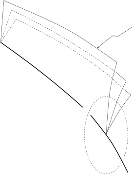
$L$$S^{1}$$f^{-1}(\varphi)$

Figure 16: An open book near the binding.

At the cost of raising the genus of the pages, one may decrease the number of components of $L$, and in particular one may always assume $L$ to be a knot. Another way to think of such an open book is as follows. Start with a surface $\Sigma$ with boundary $\partial\Sigma=K\cong S^{1}$ and a self-diffeomorphism $h$ of $\Sigma$ with $h=\mbox{\rm id}$ near $K$. Form the mapping torus $T_{h}=\Sigma_{h}=\Sigma\times[0,2\pi]/\!\!\sim$, where ‘$\sim$’ denotes the identification $(p,2\pi)\sim(h(p),0)$. Define a $3$–manifold $M$ by

$$M=T_{h}\cup_{K\times S^{1}}(K\times D^{2}).$$

This $M$ carries by construction the structure of an open book with binding $K$ and pages diffeomorphic to $\Sigma$.

Here is a slight variation on a simple argument of Thurston and Winkelnkemper [101] for producing a contact structure on such an open book (and hence on any closed, orientable $3$–manifold):

Start with a $1$–form $\beta_{0}$ on $\Sigma$ with $\beta_{0}=e^{t}d\theta$ near $\partial\Sigma=K$, where $\theta$ denotes the coordinate along $K$ and $t$ is a collar parameter with $K=\{t=0\}$ and $t<0$ in the interior of $\Sigma$. Then $d\beta_{0}$ integrates to $2\pi$ over $\Sigma$ by Stokes’s theorem. Given any area form $\omega$ on $\Sigma$ (with total area equal to $2\pi$) satisfying $\omega=e^{t}dt\wedge d\theta$ near $K$, the $2$–form $\omega-d\beta_{0}$ is, by de Rham’s theorem, an exact $1$–form, say $d\beta_{1}$, where we may assume $\beta_{1}\equiv 0$ near $K$.

Set $\beta=\beta_{0}+\beta_{1}$. Then $d\beta=\omega$ is an area form (of total area $2\pi$) on $\Sigma$ and $\beta=e^{t}d\theta$ near $K$. The set of $1$–forms satisfying these two properties is a convex set, so we can find a $1$–form (still denoted $\beta$) on $T_{h}$ which has these properties when restricted to the fibre over any $\varphi\in S^{1}=[0,2\pi]/_{0\sim 2\pi}$. We may (and shall) require that $\beta=e^{t}d\theta$ near $\partial T_{h}$.

Now a contact form $\alpha$ on $T_{h}$ is found by setting $\alpha=\beta+C\,d\varphi$ for a sufficiently large constant $C\in{\mathbb{R}}^{+}$, so that in

$$\alpha\wedge d\alpha=(\beta+C\,d\varphi)\wedge d\beta$$

the non-zero term $d\varphi\wedge d\beta=d\varphi\wedge\omega$ dominates. This contact form can be extended to all of $M$ by making the ansatz $\alpha=h_{1}(r)d\theta+h_{2}(r)d\varphi$ on $K\times D^{2}$, as described in our discussion of the Lutz twist. The boundary conditions in the present situation are, say,

• $h_{1}(r)=2$ and $h_{2}(r)=r^{2}$ near $r=0$,

• $h_{1}(r)=e^{1-r}$ and $h_{2}(r)=C$ near $r=1$.

Observe that subject to these boundary conditions a curve $(h_{1}(r),h_{2}(r))$ can be found that does not pass the $h_{2}$–axis (i.e. with $h_{1}(r)$ never being equal to zero). In the $3$–dimensional setting this is not essential (and the Thurston-Winkelnkemper ansatz lacked that feature), but it is crucial when one tries to generalise this construction to higher dimensions. This has recently been worked out by Giroux and J.-P. Mohsen [57]. This, however, is only the easy part of their work. Rather strikingly, they have shown that a converse of this result holds: Given a compact contact manifold of arbitrary dimension, it admits an open book decomposition that is adapted to the contact structure in the way described above. Full details have not been published at the time of writing, but see Giroux’s talk [56] at the ICM 2002.

3.5.2 Branched covers

A theorem of Hilden, Montesinos and Thickstun [63] states that every closed, orientable $3$–manifold $M$ admits a branched covering $\pi\colon\thinspace M\rightarrow S^{3}$ such that the upstairs branch set is a simple closed curve that bounds an embedded disc. (Moreover, the cover can be chosen $3$–fold and simple, i.e. the monodromy representation of $\pi_{1}(S^{3}-K)$, where $K$ is the branching set downstairs (a knot in $S^{3}$), represents the meridian of $K$ by a transposition in the symmetric group $S_{3}$. This, however, is not relevant for our discussion.)

It follows immediately, as announced in Section 3.3, that every closed, orientable $3$–manifold is parallelisable: First of all, $S^{3}$ is parallelisable since it carries a Lie group structure (as the unit quaternions, for instance). Given $M$ and a branched covering $\pi\colon\thinspace M\rightarrow S^{3}$ as above, there is a $3$–ball $D^{3}\subset M$ containing the upstairs branch set. Outside of $D^{3}$, the covering $\pi$ is unbranched, so the $3$–frame on $S^{3}$ can be lifted to a frame on $M-D^{3}$. The bundle $TM|_{D^{3}}$ is trivial, so the frame defined along $\partial D^{3}$ defines an element of $\mbox{\rm SO}(3)$ (cf. the footnote in the proof of Theorem 3.10). Since $\pi_{2}(\mbox{\rm SO}(3))=0$, this frame extends over $D^{3}$.

In [59], Gonzalo uses this theorem to construct a contact structure on every closed, orientable $3$–manifold $M$, in fact one with zero Euler class: Away from the branching set one can lift the standard contact structure from $S^{3}$ (which has Euler class zero: a trivialisation is given by two of the three (quaternionic) Hopf vector fields). A careful analysis of the branched covering map near the branching set then shows how to extend this contact structure over $M$ (while keeping it trivial as $2$–plane bundle).

A branched covering construction for higher-dimensional contact manifolds is discussed in [43].

3.5.3 . . . and more

The work of Giroux [52], in which he initiated the study of convex surfaces in contact $3$–manifolds, also contains a proof of Martinet’s theorem.

An entirely different proof, due to S. Altschuler [4], finds contact structures from solutions to a certain parabolic differential equation for $1$–forms on $3$–manifolds. Some of these ideas have entered into the more far-reaching work of Eliashberg and Thurston on so-called ‘confoliations’ [32], that is, $1$–forms satisfying $\alpha\wedge d\alpha\geq 0$.

3.6 Tight and overtwisted

The title of this section describes the fundamental dichotomy of contact structures in dimension $3$ that has proved seminal for the development of the field.

In order to motivate the notion of an overtwisted contact structure, as introduced by Eliashberg [21], we consider a ‘full’ Lutz twist as follows. Let $(M,\xi)$ be a contact $3$–manifold and $K\subset M$ a knot transverse to $\xi$. As before, identify $K$ with $S^{1}\times\{0\}\subset S^{1}\times D^{2}\subset M$ such that $\xi=\ker(d\theta+r^{2}d\varphi)$ on $S^{1}\times D^{2}$. Now define a new contact structure $\xi^{\prime}$ as in Section 3.4, with $(h_{1}(r),h_{2}(r))$ now as in Figure 17, that is, the boundary conditions are now

• $h_{1}(r)=1$ and $h_{2}(r)=r^{2}$ for $r\in[0,\varepsilon]\cup[1-\varepsilon,1]$

for some small $\varepsilon>0$.

$h_{1}$$1$$h_{2}$

Figure 17: A full Lutz twist.

Lemma 3.17.

A full Lutz twist does not change the homotopy class of $\xi$ as a $2$–plane field.

Proof.

Let $(h_{1}^{t}(r),h_{2}^{t}(r))$, $r,t\in[0,1]$, be a homotopy of paths such that

• $h_{1}^{0}\equiv 1,h_{2}^{0}(r)=r^{2}$,

• $h_{i}^{1}\equiv h_{i}$, $i=1,2$,

• $h_{i}^{t}(r)=h_{i}(r)$ for $r\in[0,\varepsilon]\cup[1-\varepsilon,1]$.

Let $\chi:[0,1]\rightarrow{\bf R}$ be a smooth function which is identically zero near $r=0$ and $r=1$ and $\chi(r)>0$ for $r\in[\varepsilon,1-\varepsilon]$. Then

$$\alpha_{t}=t(1-t)\chi(r)\,dr+h_{1}^{t}(r)\,d\theta+h_{2}^{t}(r)\,d\varphi$$

is a homotopy from $\alpha_{0}=d\theta+r^{2}d\varphi$ to $\alpha_{1}=h_{1}(r)\,d\theta+h_{2}(r)\,d\varphi$ through non-zero $1$–forms. This homotopy stays fixed near $r=1$, and so it defines a homotopy between $\xi$ and $\xi^{\prime}$ as $2$–plane fields. ∎

Let $r_{0}$ be the smaller of the two positive radii with $h_{2}(r_{0})=0$ and consider the embedding

$$\begin{array}[]{rccc}\phi:&D^{2}(r_{0})&\longrightarrow&S^{1}\times D^{2}\\ &(r,\varphi)&\longmapsto&(\theta(r),r,\varphi),\end{array}$$

where $\theta(r)$ is a smooth function with $\theta(r_{0})=0$, $\theta(r)>0$ for $0\leq r<r_{0}$, and $\theta^{\prime}(r)=0$ only for $r=0$. We may require in addition that $\theta(r)=\theta(0)-r^{2}$ near $r=0$. Then

$$\phi^{*}(h_{1}(r)\,d\theta+h_{2}(r)\,d\varphi)=h_{1}(r)\theta^{\prime}(r)\,dr+h_{2}(r)\,d\varphi$$

is a differential $1$–form on $D^{2}(r_{0})$ which vanishes only for $r=0$, and along $\partial D^{2}(r_{0})$ the vector field $\partial_{\varphi}$ tangent to the boundary lies in the kernel of this $1$–form, see Figure 18. In other words, the contact planes $\ker(h_{1}(r)\,d\theta+h_{2}(r)\,d\varphi)$ intersected with the tangent planes to the embedded disc $\phi(D^{2}(r_{0}))$ induce a singular $1$–dimensional foliation on this disc with the boundary of this disc as closed leaf and precisely one singular point in the interior of the disc (Figure 19; notice that the leaves of this foliation are the integral curves of the vector field $h_{1}(r)\theta^{\prime}(r)\,\partial_{\varphi}-h_{2}(r)\,\partial_{r}$). Such a disc is called an overtwisted disc.

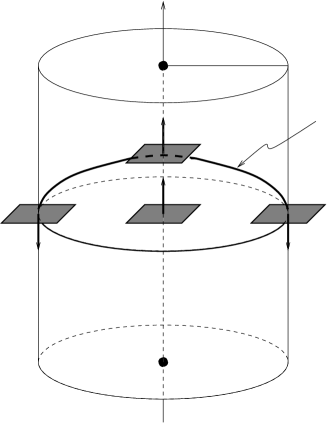
$\xi$$\phi(D^{2}(r_{0}))$$S^{1}$$r_{0}$

Figure 18: An overtwisted disc.

Figure 19: Characteristic foliation on an overtwisted disc.

A contact structure $\xi$ on a $3$–manifold $M$ is called overtwisted if $(M,\xi)$ contains an embedded overtwisted disc. In order to justify this terminology, observe that in the radially symmetric standard contact structure of Example 2.7, the angle by which the contact planes turn approaches $\pi/2$ asymptotically as $r$ goes to infinity. By contrast, any contact manifold which has been constructed using at least one (simple) Lutz twist contains a similar cylindrical region where the contact planes twist by more than $\pi$ in radial direction (at the smallest positive radius $r_{0}$ with $h_{2}(r_{0})=0$ the twisting angle has reached $\pi$).

We have shown the following

Proposition 3.18.

Let $\xi$ be a contact structure on $M$. By a full Lutz twist along any transversely embedded circle one obtains an overtwisted contact structure $\xi^{\prime}$ that is homotopic to $\xi$ as a $2$–plane distribution. $\Box$

Together with the theorem of Lutz and Martinet we find that $M$ contains an overtwisted contact structure in every homotopy class of $2$–plane distributions. In fact, Eliashberg [21] has proved the following much stronger theorem.

Theorem 3.19 (Eliashberg).

On a closed, orientable $3$–manifold there is a one-to-one correspondence between homotopy classes of overtwisted contact structures and homotopy classes of $2$–plane distributions.

This means that two overtwisted contact structures which are homotopic as $2$–plane fields are actually homotopic as contact structures and hence isotopic by Gray’s stability theorem.

Thus, it ‘only’ remains to classify contact structures that are not overtwisted. In [24] Eliashberg defined tight contact structures on a $3$–manifold $M$ as contact structures $\xi$ for which there is no embedded disc $D\subset M$ such that $D_{\xi}$ contains a limit cycle. So, by definition, overtwisted contact structures are not tight. In that same paper, as mentioned above in Section 2.4.5, Eliashberg goes on to show the converse with the help of the Elimination Lemma: non-overtwisted contact structures are tight.

There are various ways to detect whether a contact structure is tight. Historically the first proof that a certain contact structure is tight is due to D. Bennequin [9, Cor. 2, p. 150]:

Theorem 3.20 (Bennequin).

The standard contact structure $\xi_{0}$ on $S^{3}$ is tight.

The steps of the proof are as follows: (i) First, Bennequin shows that if $\gamma_{0}$ is a transverse knot in $(S^{3},\xi_{0})$ with Seifert surface $\Sigma$, then the self-linking number of $\gamma$ satisfies the inequality

$$l(\gamma_{0})\leq-\chi(\Sigma).$$

(ii) Second, he introduces an invariant for Legendrian knots; nowadays this is called the Thurston-Bennequin invariant: Let $\gamma$ be a Legendrian knot in $(S^{3},\xi_{0})$. Take a vector field $X$ along $\gamma$ transverse to $\xi_{0}$, and let $\gamma^{\prime}$ be the push-off of $\gamma$ in the direction of $X$. Then the Thurston-Bennequin invariant $tb(\gamma)$ is defined to be the linking number of $\gamma$ and $\gamma^{\prime}$. (This invariant has an extension to homologically trivial Legendrian knots in arbitrary contact $3$–manifolds.)

(iii) By pushing $\gamma$ in the direction of $\pm X$, one obtains transverse curves $\gamma^{\pm}$ (either of which is a candidate for $\gamma^{\prime}$ in (ii)). One of these curves is positively transverse, the other negatively transverse to $\xi_{0}$. The self-linking number of $\gamma^{\pm}$ is related to the Thurston-Bennequin invariant and a further invariant (the rotation number) of $\gamma$. The equation relating these three invariants implies $tb(\gamma)\leq-\chi(\Sigma)$, where $\Sigma$ again denotes a Seifert surface for $\gamma$. In particular, a Legendrian unknot $\gamma$ satisfies $tb(\gamma)<0$. This inequality would be violated by the vanishing cycle of an overtwisted disc (which has $tb=0$), which proves that $(S^{3},\xi_{0})$ is tight.

Remark 3.21.

(1) Eliashberg [25] generalised the Bennequin inequality $l(\gamma_{0})\leq-\chi(\Sigma)$ for transverse knots (and the corresponding inequality for the Thurston-Bennequin invariant of Legendrian knots) to arbitrary tight contact $3$–manifolds. Thus, whereas Bennequin established the tightness (without that name) of the standard contact structure on $S^{3}$ by proving the inequality that bears his name, that inequality is now seen, conversely, as a consequence of tightness.

(2) In [9] Bennequin denotes the positively (resp. negatively) transverse push-off of the Legendrian knot $\gamma$ by $\gamma^{-}$ (resp. $\gamma^{+}$). This has led to some sign errors in the literature. Notably, the $\pm$ in Proposition 2.2.1 of [25], relating the described invariants of $\gamma$ and $\gamma^{\pm}$, needs to be reversed.

Corollary 3.22.

The standard contact structure on ${\mathbb{R}}^{3}$ is tight.

Proof.

This is immediate from Proposition 2.13. ∎

Here are further tests for tightness:

1. A closed contact $3$–manifold $(M,\xi)$ is called symplectically fillable if there exists a compact symplectic manifold $(W,\omega)$ bounded by $M$ such that

• the restriction of $\omega$ to $\xi$ does not vanish anywhere,

• the orientation of $M$ defined by $\xi$ (i.e. the one for which $\xi$ is positive) coincides with the orientation of $M$ as boundary of the symplectic manifold $(W,\omega)$ (which is oriented by $\omega^{2}$).

We then have the following result of Eliashberg [20, Thm. 3.2.1], [22] and Gromov [62, 2.4.$D_{2}^{\prime}$(b)], cf. [10]:

Theorem 3.23 (Eliashberg-Gromov).

A symplectically fillable contact structure is tight.

Example 3.24.

The $4$–ball $D^{4}\subset{\mathbb{R}}^{4}$ with symplectic form $\omega=dx_{1}\wedge dy_{1}+dx_{2}\wedge dy_{2}$ is a symplectic filling of $S^{3}$ with its standard contact structure $\xi_{0}$. This gives an alternative proof of Bennequin’s theorem.

2. Let $(\widetilde{M},\tilde{\xi})\rightarrow(M,\xi)$ be a covering map and contactomorphism. If $(\widetilde{M},\tilde{\xi})$ is tight, then so is $(M,\xi)$, for any overtwisted disc in $(M,\xi)$ would lift to an overtwisted disc in $(\widetilde{M},\tilde{\xi})$.

Example 3.25.

The contact structures $\xi_{n}$, $n\in{\mathbb{N}}$, on the $3$–torus $T^{3}$ defined by

$$\alpha_{n}=\cos(n\theta_{1})\,d\theta_{2}+\sin(n\theta_{1})\,d\theta_{3}=0$$

are tight: Lift the contact structure $\xi_{n}$ to the universal cover ${\mathbb{R}}^{3}$ of $T^{3}$; there the contact structure is defined by the same equation $\alpha_{n}=0$, but now $\theta_{i}\in{\mathbb{R}}$ instead of $\theta_{i}\in{\mathbb{R}}/2\pi{\mathbb{Z}}\cong S^{1}$. Define a diffeomorphism $f$ of ${\mathbb{R}}^{3}$ by

$$f(x,y,z)=(y/n,z\,\cos y+x\,\sin y,z\,\sin y-x\,\cos y)=:(\theta_{1},\theta_{2},\theta_{3}).$$

Then $f^{*}\alpha_{n}=dz+x\,dy$, so the lift of $\xi_{n}$ to ${\mathbb{R}}^{3}$ is contactomorphic to the tight standard contact structure on ${\mathbb{R}}^{3}$.

Notice that it is possible for a tight contact structure to be finitely covered by an overtwisted contact structure. The first such examples were due to S. Makar-Limanov [88]. Other examples of this kind have been found by V. Colin [18] and R. Gompf [58].

3. The following theorem of H. Hofer [65] relates the dynamics of the Reeb vector field to overtwistedness.

Theorem 3.26 (Hofer).

Let $\alpha$ be a contact form on a closed $3$–manifold such that the contact structure $\ker\alpha$ is overtwisted. Then the Reeb vector field of $\alpha$ has at least one contractible periodic orbit.

Example 3.27.

The Reeb vector field $R_{n}$ of the contact form $\alpha_{n}$ of the preceding example is

$$R_{n}=\cos(n\theta_{1})\,\partial_{\theta_{2}}+\sin(n\theta_{1})\,\partial_{\theta_{3}}.$$

Thus, the orbits of $R_{n}$ define constant slope foliations of the $2$–tori $\{\theta_{1}=\mbox{\rm const.}\}$; in particular, the periodic orbits of $R_{n}$ are even homologically non-trivial. It follows, again, that the $\xi_{n}$ are tight contact structures on $T^{3}$. (This, admittedly, amounts to attacking starlings with rice puddings fired from catapults.)

3.7 Classification results

In this section I summarise some of the known classification results for contact structures on $3$–manifolds. By Eliashberg’s Theorem 3.19 it suffices to list the tight contact structures, up to isotopy or diffeomorphism, on a given closed $3$–manifold.

Theorem 3.28 (Eliashberg [24]).

Any tight contact structure on $S^{3}$ is isotopic to the standard contact structure $\xi_{0}$.

This theorem has a remarkable application in differential topology, viz., it leads to a new proof of Cerf’s theorem [16] that any diffeomorphism of $S^{3}$ extends to a diffeomorphism of the $4$–ball $D^{4}$. The idea is that the above theorem implies that any diffeomorphism of $S^{3}$ is isotopic to a contactomorphism of $\xi_{0}$. Eliashberg’s technique [22] of filling by holomorphic discs can then be used to show that such a contactomorphism extends to a diffeomorphism of $D^{4}$.

As remarked earlier (Remark 2.21), Eliashberg has also classified contact structures on ${\mathbb{R}}^{3}$. Recall that homotopy classes of $2$–plane distributions on $S^{3}$ are classified by $\pi_{3}(S^{2})\cong{\mathbb{Z}}$. By Theorem 3.19, each of these classes contains a unique (up to isotopy) overtwisted contact structure. When a point of $S^{3}$ is removed, each of these contact structures induces one on ${\mathbb{R}}^{3}$, and Eliashberg [25] shows that they remain non-diffeomorphic there. Eliashberg shows further that, apart from this integer family of overtwisted contact structures, there is a unique tight contact structure on ${\mathbb{R}}^{3}$ (the standard one), and a single overtwisted one that is ‘overtwisted at infinity’ and cannot be compactified to a contact structure on $S^{3}$.

In general, the classification of contact structures up to diffeomorphism will differ from the classification up to isotopy. For instance, on the $3$–torus $T^{3}$ we have the following diffeomorphism classification due to Y. Kanda [75]:

Theorem 3.29 (Kanda).

Every (positive) tight contact structure on $T^{3}$ is contactomorphic to one of the $\xi_{n}$, $n\in{\mathbb{N}}$, described above. For $n\neq m$, the contact structures $\xi_{n}$ and $\xi_{m}$ are not contactomorphic.

Giroux [54] had proved earlier that $\xi_{n}$ for $n\geq 2$ is not contactomorphic to $\xi_{1}$.

On the other hand, all the $\xi_{n}$ are homotopic as $2$–plane fields to $\{d\theta_{1}=0\}$. This shows one way how Eliashberg’s classification Theorem 3.19 for overtwisted contact structures can fail for tight contact structures:

• There are tight contact structures on $T^{3}$ that are homotopic as plane fields but not contactomorphic.

P. Lisca and G. Matić [82] have found examples of the same kind on homology spheres by applying Seiberg-Witten theory to Stein fillings of contact manifolds, cf. also [78].

Eliashberg and L. Polterovich [31] have determined the isotopy classes of diffeomorphisms of $T^{3}$ that contain a contactomorphism of $\xi_{1}$: they correspond to exactly those elements of $\mbox{\rm SL}(3,{\mathbb{Z}})=\pi_{0}(\mbox{\rm Diff}(T^{3}))$ that stabilise the subspace $0\oplus{\mathbb{Z}}^{2}$ corresponding to the coordinates $(\theta_{2},\theta_{3})$. In combination with Kanda’s result, this allows to give an isotopy classification of tight contact structures on $T^{3}$. One particular consequence of the result of Eliashberg and Polterovich is the following:

• There are tight contact structures on $T^{3}$ that are contactomorphic and homotopic as plane fields, but not isotopic (i.e. not homotopic through contact structures).

Again, such examples also exist on homology spheres, as S. Akbulut and R. Matveyev [2] have shown.

Another aspect of Eliashberg’s classification of overtwisted contact structures that fails to hold for tight structures is of course the existence of such a structure in every homotopy class of $2$–plane fields, as is already demonstrated by the classification of contact structures on $S^{3}$. Etnyre and K. Honda [37] have recently even found an example of a manifold – the connected some of two copies of the Poincaré sphere with opposite orientations – that does not admit any tight contact structure at all.

For the classification of tight contact structures on lens spaces and $T^{2}$–bundles over $S^{1}$ see [55], [71] and [72]. A partial classification of tight contact structures on lens spaces had been obtained earlier in [34].

As further reading on $3$–dimensional contact geometry I can recommend the lucid Bourbaki talk by Giroux [53]. This covers the ground up to Eliashberg’s classification of overtwisted contact structures and the uniqueness of the tight contact structure on $S^{3}$.

4 A guide to the literature

In this concluding section I give some recommendations for further reading, concentrating on those aspects of contact geometry that have not (or only briefly) been touched upon in earlier sections.

Two general surveys that emphasise historical matters and describe the development of contact geometry from some of its earliest origins are the one by Lutz [87] and one by the present author [45].

One aspect of contact geometry that I have neglected in these notes is the Riemannian geometry of contact manifolds (leading, for instance, to Sasakian geometry). The survey by Lutz has some material on that; D. Blair [11] has recently published a monograph on the topic.

There have also been various ideas for defining interesting families of contact structures. Again, the survey by Lutz has something to say on that; one such concept that has exhibited very intriguing ramifications – if this commercial break be permitted – was introduced in [48].

4.1 Dimension $3$

As mentioned earlier, Chapter 8 in [1] is in parts complementary to the present notes and has some material on surfaces in contact $3$–manifolds. Other surveys and introductory texts on $3$–dimensional contact geometry are the introductory lectures by Etnyre [35] and the Bourbaki talk by Giroux [52]. Good places to start further reading are two papers by Eliashberg: [24] for the classification of tight contact structures and [26] for knots in contact $3$–manifolds. Concerning the latter, there is also a chapter in preparation by Etnyre [36] for a companion Handbook and an article by Etnyre and Honda [38] with an extensive introduction to that subject.

The surveys [20] and [27] by Eliashberg are more general in scope, but also contain material about contact $3$–manifolds.

$3$–dimensional contact topology has now become a fairly wide arena; apart from the work of Eliashberg, Giroux, Etnyre-Honda and others described earlier, I should also mention the results of Colin, who has, for instance, shown that surgery of index one (in particular: taking the connected sum) on a tight contact $3$–manifold leads again to a tight contact structure [17].

Finally, Etnyre and L. Ng [40] have compiled a useful list of problems in $3$–dimensional contact topology.

4.2 Higher dimensions

The article [46] by the present author contains a survey of what was known at the time of writing about the existence of contact structures on higher-dimensional manifolds. One of the most important techniques for constructing contact manifolds in higher dimensions is the so-called contact surgery along isotropic spheres developed by Eliashberg [23] and A. Weinstein [105]. The latter is a very readable paper. For a recent application of this technique see [49]. Other constructions of contact manifolds (branched covers, gluing along codimension $2$ contact submanifolds) are described in my paper [43].

Odd-dimensional tori are of course amongst the manifolds with the simplest global description, but they do not easily lend themselves to the construction of contact structures. In [86] Lutz found a contact structure on $T^{5}$; since then it has been one of the prize questions in contact geometry to find a contact structure on higher-dimensional tori. That prize, as it were, recently went to F. Bourgeois [13], who showed that indeed all odd-dimensional tori do admit a contact structure. His construction uses the result of Giroux and Mohsen [56], [57] about open book decompositions adapted to contact structures in conjunction with the original proof of Lutz. With the help of the branched cover theorem described in [43] one can conclude further that every manifold of the form $M\times{\Sigma}$ with $M$ a contact manifold and $\Sigma$ a surface of genus at least $1$ admits a contact structure.

Concerning the classification of contact structures in higher dimensions, the first steps have been taken by Eliashberg [28] with the development of contact homology, which has been taken further in [29]. This has been used by I. Ustilovsky [102] to show that on $S^{4n+1}$ there exist infinitely many non-isomorphic contact structures that are homotopically equivalent (in the sense that they induce the same almost contact structure, i.e. reduction of the structure group of $TS^{4n+1}$ to $1\times\mbox{\rm U}(2n)$). Earlier results in this direction can be found in [44] in the context of various applications of contact surgery.

4.3 Symplectic fillings

A survey on the various types of symplectic fillings of contact manifolds is given by Etnyre [33], cf. also the survey by Bennequin [10]. Etnyre and Honda [39] have recently shown that certain Seifert fibred $3$–manifolds $M$ admit tight contact structures $\xi$ that are not symplectically semi-fillable, i.e. there is no symplectic filling $W$ of $(M,\xi)$ even if $W$ is allowed to have other contact boundary components. That paper also contains a good update on the general question of symplectic fillability.

A related question is whether symplectic manifolds can have disconnected boundary of contact type (this corresponds to a stronger notion of symplectic filling defined via a Liouville vector field transverse to the boundary and pointing outwards). For (boundary) dimension $3$ this is discussed by D. McDuff [91]; higher-dimensional symplectic manifolds with disconnected boundary of contact type have been constructed in [42].

4.4 Dynamics of the Reeb vector field

In a seminal paper, Hofer [65] applied the method of pseudo-holomorphic curves, which had been introduced to symplectic geometry by Gromov [62], to solve (for large classes of contact $3$–manifolds) the so-called Weinstein conjecture [104] concerning the existence of periodic orbits of the Reeb vector field of a given contact form. (In fact, one of the remarkable aspects of Hofer’s work is that in many instances it shows the existence of a periodic orbit of the Reeb vector field of any contact form defining a given contact structure.) A Bourbaki talk on the state of the art around the time when Weinstein formulated the conjecture that bears his name was given by N. Desolneux-Moulis [19]; another Bourbaki talk by F. Laudenbach describes Hofer’s contribution to the problem.

The textbook by Hofer and E. Zehnder [70] addresses these issues, although its main emphasis, as is clear from the title, lies more in the direction of symplectic geometry and Hamiltonian dynamics. Two surveys by Hofer [66], [67], and one by Hofer and M. Kriener [68], are more directly concerned with contact geometry. Of the three, [66] may be the best place to start, since it derives from a course of five lectures. In collaboration with K. Wysocki and Zehnder, Hofer has expanded his initial ideas into a far-reaching project on the characterisation of contact manifolds via the dynamics of the Reeb vector field, see e.g. [69].

References

- [1] B. Aebischer, M. Borer, M. Kälin, Ch. Leuenberger and H.M. Reimann, Symplectic Geometry, Progr. Math. 124, Birkhäuser, Basel (1994).
- [2] S. Akbulut and R. Matveyev, A note on contact structures, Pacific J. Math. 182 (1998), 201–204.
- [3] D.N. Akhiezer, Homogeneous complex manifolds, in: Several Complex Variables IV (S.G. Gindikin, G.M. Khenkin, eds.), Encyclopaedia Math. Sci. 10, Springer, Berlin (1990), 195–244.
- [4] S. Altschuler, A geometric heat flow for one-forms on three-dimensional manifolds, Illinois J. Math. 39 (1995), 98–118.
- [5] J.W. Alexander, A lemma on systems of knotted curves, Proc. Nat. Acad. Sci. U.S.A. 9 (1923), 93–95.
- [6] V.I. Arnold, Characteristic class entering in quantization conditions, Funct. Anal. Appl. 1 (1967), 1–13.
- [7] V.I. Arnold, Mathematical Methods of Classical Mechanics, Grad. Texts in Math. 60, Springer, Berlin (1978).
- [8] A. Banyaga, The Structure of Classical Diffeomorphism Groups, Math. Appl. 400, Kluwer, Dordrecht (1997).
- [9] D. Bennequin, Entrelacements et équations de Pfaff, in: IIIe Rencontre de Géométrie du Schnepfenried, vol. 1, Astérisque 107–108 (1983), 87–161.
- [10] D. Bennequin, Topologie symplectique, convexité holomorphe et structures de contact (d’après Y. Eliashberg, D. McDuff et al.), in: Séminaire Bourbaki, vol. 1989/90, Astérisque 189–190 (1990), 285–323.
- [11] D.E. Blair, Riemannian Geometry of Contact and Symplectic Manifolds, Progr. Math. 203, Birkhäuser, Basel (2002).
- [12] W.M. Boothby, Transitivity of the automorphisms of certain geometric structures, Trans. Amer. Math. Soc. 137 (1969), 93–100.
- [13] F. Bourgeois, Odd dimensional tori are contact manifolds, Int. Math. Res. Notices 2002, 1571–1574.
- [14] G.E. Bredon, Topology and Geometry, Grad. Texts in Math. 139, Springer, Berlin (1993).
- [15] Th. Bröcker and K. Jänich, Einführung in die Differentialtopologie, Springer, Berlin (1973).
- [16] J. Cerf, Sur les difféomorphismes de la sphère de dimension trois (), Lecture Notes in Math. 53, Springer, Berlin (1968).
- [17] V. Colin, Chirurgies d’indice un et isotopies de sphères dans les variétés de contact tendues, C. R. Acad. Sci. Paris Sér. I Math. 324 (1997), 659–663.
- [18] V. Colin, Recollement de variétés de contact tendues, Bull. Soc. Math. France 127 (1999), 43–69.
- [19] N. Desolneux-Moulis, Orbites périodiques des systèmes hamiltoniens autonomes (d’après Clarke, Ekeland-Lasry, Moser, Rabinowitz, Weinstein), in: Séminaire Bourbaki, vol. 1979/80, Lecture Notes in Math. 842, Springer, Berlin (1981), 156–173.
- [20] Y. Eliashberg, Three lectures on symplectic topology in Cala Gonone: Basic notions, problems and some methods, in: Conference on Differential Geometry and Topology (Sardinia, 1988), Rend. Sem. Fac. Sci. Univ. Cagliari 58 (1988), suppl., 27–49.
- [21] Y. Eliashberg, Classification of overtwisted contact structures on –manifolds, Invent. Math. 98 (1989), 623–637.
- [22] Y. Eliashberg, Filling by holomorphic discs and its applications, in: Geometry of Low-Dimensional Manifolds (Durham, 1989) vol. 2, London Math. Soc. Lecture Note Ser. 151, Cambridge University Press (1990), 45–67.
- [23] Y. Eliashberg, Topological characterization of Stein manifolds of dimension , Internat. J. Math. 1 (1990), 29–46.
- [24] Y. Eliashberg, Contact –manifolds twenty years since J. Martinet’s work, Ann. Inst. Fourier (Grenoble) 42 (1992), no. 1-2, 165–192.
- [25] Y. Eliashberg, Classification of contact structures on , Internat. Math. Res. Notices 1993, 87–91.
- [26] Y. Eliashberg, Legendrian and transversal knots in tight contact –manifolds, in: Topological Methods in Modern Mathematics (Stony Brook, 1991), Publish or Perish, Houston (1993), 171–193.
- [27] Y. Eliashberg, Symplectic topology in the nineties, Differential Geom. Appl. 9 (1998), 59–88.
- [28] Y. Eliashberg, Invariants in contact topology, in: Proceedings of the International Congress of Mathematicians (Berlin, 1998) vol. II, Doc. Math. 1998, Extra Vol. II, 327–338.
- [29] Y. Eliashberg, A. Givental and H. Hofer, Introduction to symplectic field theory, Geom. Funct. Anal. 2000, Special Volume, Part II, 560–673.
- [30] Y. Eliashberg and N. Mishachev, Introduction to the -principle, Grad. Stud. Math. 48, American Mathematical Society, Providence (2002).
- [31] Y. Eliashberg and L. Polterovich, New applications of Luttinger’s surgery, Comment. Math. Helv. 69 (1994), 512–522.
- [32] Y. Eliashberg and W.P. Thurston, Confoliations, Univ. Lecture Ser. 13, American Mathematical Society, Providence (1998).
- [33] J.B. Etnyre, Symplectic convexity in low-dimensional topology, Topology Appl. 88 (1998), 3–25.
- [34] J.B. Etnyre, Tight contact structures on lens spaces, Commun. Contemp. Math. 2 (2000), 559–577; erratum: ibid. 3 (2001), 649–652.
- [35] J.B. Etnyre, Introductory lectures on contact geometry, in: Proc. Georgia Topology Conference (Athens, GA, 2001), to appear.
- [36] J.B. Etnyre, chapter in preparation for Handbook of Knot Theory (W. Menasco, M. Thistlethwaite, eds.).
- [37] J.B. Etnyre and K. Honda, On the nonexistence of tight contact structures, Ann. of Math. (2) 153 (2001), 749–766.
- [38] J.B. Etnyre and K. Honda, Knots and contact geometry I: Torus knots and the figure eight knot, J. Symplectic Geom. 1 (2001), 63–120.
- [39] J.B. Etnyre and K. Honda, Tight contact structures with no symplectic fillings, Invent. Math. 148 (2002), 609–626.
- [40] J.B. Etnyre and L.L. Ng, Problems in low-dimensional contact topology, in: Proc. Georgia Topology Conference (Athens, GA, 2001), to appear.
- [41] H. Freudenthal, Zum Hopfschen Umkehrhomomorphismus, Ann. of Math. (2) 38 (1937), 847–853.
- [42] H. Geiges, Symplectic manifolds with disconnected boundary of contact type, Internat. Math. Res. Notices 1994, 23–30.
- [43] H. Geiges, Constructions of contact manifolds, Math. Proc. Cambridge Philos. Soc. 121 (1997), 455–464.
- [44] H. Geiges, Applications of contact surgery, Topology 36 (1997), 1193–1220.
- [45] H. Geiges, A brief history of contact geometry and topology, Expo. Math. 19 (2001), 25–53.
- [46] H. Geiges, Contact topology in dimension greater than three, in: European Congress of Mathematics (Barcelona, 2000) vol. 2, Progress in Math. 202, Birkhäuser, Basel (2001), 535–545.
- [47] H. Geiges, -Principles and flexibility in geometry, Mem. Amer. Math. Soc. 164 (2003), no. 779.
- [48] H. Geiges and J. Gonzalo, Contact geometry and complex surfaces, Invent. Math. 121 (1995), 147–209.
- [49] H. Geiges and C.B. Thomas, Contact structures, equivariant spin bordism, and periodic fundamental groups, Math. Ann. 320 (2001), 685–708.
- [50] V.L. Ginzburg, On closed characteristics of –forms, Ph.D. Thesis, Berkeley (1990).
- [51] V.L. Ginzburg, Calculation of contact and symplectic cobordism groups, Topology 31 (1992), 767–773.
- [52] E. Giroux, Convexité en topologie de contact, Comment. Math. Helv. 66 (1991), 637–677.
- [53] E. Giroux, Topologie de contact en dimension (autour des travaux de Yakov Eliashberg), in: Séminaire Bourbaki, vol. 1992/93, Astérisque 216 (1993), 7–33.
- [54] E. Giroux, Une structure de contact, même tendue, est plus ou moins tordue, Ann. Sci. École Norm. Sup. (4) 27 (1994), 697–705.
- [55] E. Giroux, Structures de contact en dimension trois et bifurcations des feuilletages de surfaces, Invent. Math. 141 (2000), 615–689.
- [56] E. Giroux, Géométrie de contact: de la dimension trois vers les dimensions supérieures, in: Proceedings of the International Congress of Mathematicians (Beijing, 2002) vol. II, Higher Education Press, Beijing (2002), 405–414.
- [57] E. Giroux and J.-P. Mohsen, Structures de contact et fibrations symplectiques au-dessus du cercle, in preparation.
- [58] R.E. Gompf, Handlebody construction of Stein surfaces, Ann. of Math. (2) 148 (1998), 619–693.
- [59] J. Gonzalo, Branched covers and contact structures, Proc. Amer. Math. Soc. 101 (1987), 347–352.
- [60] D.H. Gottlieb, Partial transfers, in: Geometric Applications of Homotopy Theory I, Lecture Notes in Math. 657, Springer, Berlin (1978), 255–266.
- [61] J.W. Gray, Some global properties of contact structures, Ann. of Math. (2) 69 (1959), 421–450.
- [62] M. Gromov, Pseudoholomorphic curves in symplectic manifolds, Invent. Math. 82 (1985), 307–347.
- [63] H.M. Hilden, J.M. Montesinos and T. Thickstun, Closed oriented –manifolds as –fold branched coverings of of special type, Pacific J. Math. 65 (1976), 65–76.
- [64] M.W. Hirsch, Differential Topology, Grad. Texts in Math. 33, Springer, Berlin (1976).
- [65] H. Hofer, Pseudoholomorphic curves in symplectizations with applications to the Weinstein conjecture in dimension , Invent. Math. 114 (1993), 515–563.
- [66] H. Hofer, Holomorphic curves and dynamics in dimension three, in: Symplectic Geometry and Topology (Park City, 1997), IAS/Park City Math. Ser. 7, American Mathematical Society, Providence (1999), 35–101.
- [67] H. Hofer, Holomorphic curves and real three-dimensional dynamics, Geom. Funct. Anal. 2000, Special Volume, Part II, 674–704.
- [68] H. Hofer and M. Kriener, Holomorphic curves in contact dynamics, in: Differential Equations (La Pietra, 1996), Proc. Sympos. Pure Math. 65, American Mathematical Society, Providence (1999), 77–131.
- [69] H. Hofer, K. Wysocki and E. Zehnder, A characterisation of the tight three-sphere, Duke Math. J. 81 (1995), 159–226; erratum: ibid. 89 (1997), 603–617.
- [70] H. Hofer and E. Zehnder, Symplectic Invariants and Hamiltonian Dynamics Birkhäuser, Basel (1994).
- [71] K. Honda, On the classification of tight contact structures I, Geom. Topol. 4 (2000), 309–368.
- [72] K. Honda, On the classification of tight contact structures II, J. Differential Geom. 55 (2000), 83–143.
- [73] H. Hopf, Zur Algebra der Abbildungen von Mannigfaltigkeiten, J. Reine Angew. Math. 105 (1930), 71–88.
- [74] D. Husemoller, Fibre Bundles (3rd edition), Grad. Texts in Math. 20, Springer, Berlin (1994).
- [75] Y. Kanda, The classification of tight contact structures on the –torus, Comm. Anal. Geom. 5 (1997), 413–438.
- [76] R.C. Kirby, The Topology of –Manifolds, Lecture Notes in Math. 1374, Springer, Berlin (1989).
- [77] A.A. Kosinski, Differential Manifolds, Academic Press, Boston (1993).
- [78] P.B. Kronheimer and T.S. Mrowka, Monopoles and contact structures, Invent. Math. 130 (1997), 209–255.
- [79] F. Laudenbach, Orbites périodiques et courbes pseudo-holomorphes, application à la conjecture de Weinstein en dimension (d’après H. Hofer et al.), in: Séminaire Bourbaki, vol. 1993/1994, Astérisque 227 (1995), 309–333.
- [80] P. Libermann and C.-M. Marle, Symplectic Geometry and Analytical Mechanics, Math. Appl. 35, Reidel, Dordrecht (1987).
- [81] W.B.R. Lickorish, A representation of orientable combinatorial –manifolds, Ann. of Math. (2) 76 (1962), 531–540.
- [82] P. Lisca and G. Matić, Tight contact structures and Seiberg-Witten invariants, Invent. Math. 129 (1997), 509–525.
- [83] R. Lutz, Sur l’existence de certaines formes différentielles remarquables sur la sphère , C. R. Acad. Sci. Paris Sér. A–B 270 (1970), A1597–A1599.
- [84] R. Lutz, Sur quelques propriétés des formes differentielles en dimension trois, Thèse, Strasbourg (1971).
- [85] R. Lutz, Structures de contact sur les fibrés principaux en cercles de dimension trois, Ann. Inst. Fourier (Grenoble), 27 (1977), no. 3, 1–15.
- [86] R. Lutz, Sur la géométrie des structures de contact invariantes, Ann. Inst. Fourier (Grenoble) 29 (1979), no. 1, 283–306.
- [87] R. Lutz, Quelques remarques historiques et prospectives sur la géométrie de contact, in: Conference on Differential Geometry and Topology (Sardinia, 1988), Rend. Sem. Fac. Sci. Univ. Cagliari 58 (1988), suppl., 361–393.
- [88] S. Makar-Limanov, Tight contact structures on solid tori, Trans. Amer. Math. Soc. 350 (1998), 1013–1044.
- [89] J. Martinet, Sur les singularités des formes différentielles, Ann Inst. Fourier (Grenoble) 20 (1970) no. 1, 95–178.
- [90] J. Martinet, Formes de contact sur les variétés de dimension , in: Proc. Liverpool Singularities Sympos. II, Lecture Notes in Math. 209, Springer, Berlin (1971), 142–163.
- [91] D. McDuff, Symplectic manifolds with contact type boundaries, Invent. Math. 103 (1991), 651–671.
- [92] D. McDuff and D. Salamon, Introduction to Symplectic Topology (2nd edition), Oxford University Press, 1998.
- [93] S. Milligan, The Starlings, in: The Goon Show, Series 4, Special Programme, broadcast 31st August 1954.
- [94] J.W. Milnor, Topology from the Differentiable Viewpoint, The University Press of Virginia, Charlottesville (1965).
- [95] J.W. Milnor and J.D. Stasheff, Characteristic Classes, Annals of Math. Studies 76, Princeton University Press, Princeton (1974).
- [96] J. Moser, On the volume elements on a manifold, Trans. Amer. Math. Soc. 120 (1965), 286–294.
- [97] D. Rolfsen, Knots and Links, Publish or Perish, Houston (1976).
- [98] N. Saveliev, Lectures on the Topology of –Manifolds, de Gruyter, Berlin (1999).
- [99] N. Steenrod, The Topology of Fibre Bundles, Princeton University Press, Princeton (1951).
- [100] I. Tamura, Topology of Foliations: An Introduction, Transl. Math. Monogr. 97, American Mathematical Society, Providence, 1992.
- [101] W.P. Thurston and H.E. Winkelnkemper, On the existence of contact forms, Proc. Amer. Math. Soc. 52 (1975), 345–347.
- [102] I. Ustilovsky, Infinitely many contact structures on , Internat. Math. Res. Notices 1999, 781–791.
- [103] A.H. Wallace, Modifications and cobounding manifolds, Canad. J. Math. 12 (1960), 503–528.
- [104] A. Weinstein, On the hypotheses of Rabinowitz’ periodic orbit theorem, J. Differential Equations 33 (1979), 353–358.
- [105] A. Weinstein, Contact surgery and symplectic handlebodies, Hokkaido Math. J. 20 (1991), 241–251.