Surgery diagrams for contact $3$-manifolds

Abstract.

In two previous papers, the two first-named authors introduced a notion of contact $r$-surgery along Legendrian knots in contact $3$-manifolds. They also showed how (at least in principle) to convert any contact $r$-surgery into a sequence of contact $(\pm 1)$-surgeries, and used this to prove that any (closed) contact $3$-manifold can be obtained from the standard contact structure on $S^{3}$ by a sequence of such contact $(\pm 1)$-surgeries.

In the present paper, we give a shorter proof of that result and a more explicit algorithm for turning a contact $r$-surgery into $(\pm 1)$-surgeries. We use this to give explicit surgery diagrams for all contact structures on $S^{3}$ and $S^{1}\times S^{2}$, as well as all overtwisted contact structures on arbitrary closed, orientable $3$-manifolds. This amounts to a new proof of the Lutz-Martinet theorem that each homotopy class of $2$-plane fields on such a manifold is represented by a contact structure.

1. Introduction

Let $Y$ be a closed, orientable $3$-manifold. A coorientable contact structure on $Y$ is the kernel $\xi=\ker\alpha$ of a differential $1$-form on $Y$ with the property that $\alpha\wedge d\alpha$ is a volume form. Fixing a coorientation of $\xi$ amounts to fixing $\alpha$ up to multiplication with a postive function. In the sequel, we shall assume implicitly that our contact structures are cooriented; moreover, we equip $Y$ with the orientation induced by the volume form $\alpha\wedge d\alpha$. This ensures that when below we realise certain $(Y,\xi)$ as the boundary of an almost complex $4$-manifold $(X,J)$, the orientation of $Y$ induced by $\xi$ coincides with the orientation of $Y$ as the boundary of the manifold $X$ (oriented by $J$).

The standard contact structure $\xi_{st}$ on the $3$-sphere $S^{3}\subset{\mathbb{R}}^{4}$ (with cartesian coordinates $x,y,z,t$) is defined as the kernel of

$$\alpha_{st}=x\,dy-y\,dx+z\,dt-t\,dz$$

or, equivalently, as the complex tangencies of $S^{3}\subset{\mathbb{C}}^{2}$. For other basics of contact geometry we refer to [5]; for Legendrian knots and their presentation via front projections see [12], [8]; for the general differential topological background of contact geometry see [11].

A Legendrian knot $K$ in a contact $3$-manifold $(Y,\xi)$ is a knot that is everywhere tangent to $\xi$. Such knots come with a canonical contact framing, defined by a vector field along $K$ that is transverse to $\xi$. Recall that $(Y,\xi)$ is called overtwisted if it contains an embedded disc $D^{2}\subset Y$ with boundary $\partial D^{2}$ a Legendrian knot whose contact framing equals the framing it receives from the disc $D^{2}$. If no such disc exists, the contact structure is called tight.

In [1] a notion of contact $r$-surgery along a Legendrian knot $K$ in a contact manifold $(Y,\xi)$ was described: This amounts to a topological surgery, with surgery coefficient $r\in{\mathbb{Q}}\cup{\infty}$ measured relative to the contact framing. A contact structure on the surgered manifold

$$(Y-\nu K)\cup(S^{1}\times D^{2}),$$

with $\nu K$ denoting a tubular neighbourhood of $K$, is defined, for $r\neq 0$, by requiring this contact structure to coincide with $\xi$ on $Y-\nu K$ and its extension over $S^{1}\times D^{2}$ to be tight (on $S^{1}\times D^{2}$, not necessarily the whole surgered manifold). According to [14], such an extension always exists and is unique (up to isotopy) for $r=1/k$ with $k\in{\mathbb{Z}}$. (For $r=0$, that extension is necessarily overtwisted and thus requires a different treatment. For that reason we shall not discuss the case of $0$-surgery any further in the present paper.) Therefore, if $r=1/k$ with $k\in{\mathbb{Z}}$, there is a canonical procedure for this surgery, that is, the resulting contact structure on the surgered manifold is completely determined by the initial manifold $(Y,\xi)$, the Legendrian knot $K$ in $Y$, and the surgery coefficient $r=1/k$.

A contact $(-1)$-surgery corresponds to a symplectic handlebody surgery in the sense of [4], [20] (cf. also Remark 3.3 below). For future reference we record the following lemma, see [1, Prop. 8], [2, Section 3]:

Lemma 1.1.

Contact $(-1)$-surgery along a Legendrian knot $K\subset(Y,\xi)$ and contact $(+1)$-surgery along a Legendrian push-off of $K$ cancel each other.

In [2] the following has been proved:

Theorem 1.2 ([2]).

Every (closed, orientable) contact $3$-manifold $(Y,\xi)$ can be obtained via contact $(\pm 1)$-surgery on a Legendrian link in $(S^{3},\xi_{st})$.

A simple way of proving this theorem relies on the following result of Etnyre and Honda:

Theorem 1.3 ([9]).

Let $(Y_{i},\xi_{i})$ ($i=1,2$) be two given contact $3$-manifolds and suppose that $(Y_{1},\xi_{1})$ is overtwisted. Then there is a Legendrian link ${\mathbb{L}}\subset(Y_{1},\xi_{1})$ such that contact $(-1)$-surgery on ${\mathbb{L}}$ produces $(Y_{2},\xi_{2})$. ∎

Proof of Theorem 1.2.

Let $(Y_{2},\xi_{2})=(Y,\xi)$ be given. Let $(Y_{1},\xi_{1})$ be the contact manifold obtained by contact $(+1)$-surgery on the Legendrian knot $K$ in $(S^{3},\xi_{st})$ shown in Figure 1.

$+1$

Figure 1. Legendrian knot producing an overtwisted $S^{3}$.

That Legendrian knot $K$ has Thurston-Bennequin invariant $-2$, that is, the longitude $\lambda_{c}$ given by the contact framing is related (homotopically) to the meridian $\mu$ and standard longitude $\lambda$ of $K$ (with linking number $\ell k\,(\lambda,K)=0$) by $\lambda_{c}=\lambda-2\mu$. Thus, contact $(+1)$-surgery along $K$ means that we cut out a tubular neighbourhood of $K$ and glue in a solid torus by sending its meridian to $\lambda_{c}+\mu=\lambda-\mu$, which amounts to a topological $(-1)$-surgery with respect to the standard framing given by $\lambda$. Such a surgery is topologically trivial, that is, $Y_{1}=S^{3}$.

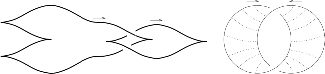
$+1$$K$$K^{\prime}$$K$$K^{\prime}$

Figure 2. The overtwisted disc in $(S^{3},\xi_{1}$).

Figure 2 shows that $(S^{3},\xi_{1})$ is overtwisted: The surface framing of $K$ determined by the Seifert surface $\Sigma$ of the Hopf link $K\sqcup K^{\prime}$ shown in that figure is $-1$, hence equal to the framing used for the surgery. This implies that the new meridional disc $D_{m}$ in the surgered manifold and $\Sigma$ glued together define an embedded disc $D_{0}=D_{m}\cup_{K}\Sigma$ in the surgered manifold. The surface framing of $K^{\prime}$ determined by $D_{0}$ is $-1$, which equals the contact framing of $K^{\prime}$. Hence $D_{0}$ is an overtwisted disc.

It follows that Theorem 1.3 applies and yields the desired surgery presentation. ∎

Notice that, in fact, we have obtained a slightly stronger statement:

Corollary 1.4.

Let $(Y,\xi)$ be a contact $3$-manifold. Then there is a Legendrian link ${\mathbb{L}}\subset(S^{3},\xi_{st})$ and a Legendrian knot $K\subset(S^{3},\xi_{st})$ disjoint from ${\mathbb{L}}$ such that contact $(+1)$-surgery on $K$ and contact $(-1)$-surgery on ${\mathbb{L}}$ yield $(Y,\xi)$. ∎

In other words, we can assume that in the surgery presentation we have a single knot on which we do contact $(+1)$-surgery. As the proof shows, this $K\subset(S^{3},\xi_{st})$ can be chosen arbitrarily as long as $(+1)$-surgery on it results in an overtwisted structure. Needless to say, different choices for $K$ necessitate different Legendrian links ${\mathbb{L}}$ for the $(-1)$-surgeries.

Corollary 1.5.

For a contact $3$-manifold $(Y,\xi)$ there is a Legendrian knot $K^{*}$ such that $(Y-\nu K^{*},\xi|_{Y-\nu K^{*}})$, the complement of a tubular neighbourhood $\nu K^{*}$ of $K^{*}$, embeds into a Stein fillable contact $3$-manifold. In particular, $(Y-\nu K^{*},\xi|_{Y-\nu K^{*}})$ is tight.

Proof.

Let $(Y^{\prime},\xi^{\prime})$ be the contact manifold obtained by performing the contact $(-1)$-surgeries along ${\mathbb{L}}$. This is a Stein fillable manifold. Our manifold $(Y,\xi)$ is obtained from $(Y^{\prime},\xi^{\prime})$ by a contact $(+1)$-surgery along $K$ (which we may regard as a Legendrian knot in $(Y^{\prime},\xi^{\prime})$), that is,

$$(Y,\xi)=(Y^{\prime}-\nu K,\xi^{\prime}|_{Y^{\prime}-\nu K})\cup(S^{1}\times D^{2}),$$

where $\xi$ is defined by the unique extension of $\xi^{\prime}$ over $S^{1}\times D^{2}$ as a tight contact structure on that solid torus. For a contact $(+1)$-surgery, that contact structure on $S^{1}\times D^{2}$ is the unique contact structure on the tubular neighbourhood $\nu K^{*}$ of a Legendrian knot $K^{*}$. So we may think of $K^{*}$ as a Legendrian knot in $(Y,\xi)$ and identify $(Y-\nu K^{*},\xi|_{Y-\nu K^{*}})$ with $(Y^{\prime}-\nu K,\xi^{\prime}|_{Y^{\prime}-\nu K})$. ∎

Remark 1.6.

The proof of Theorem 1.3 proceeds roughly as follows: If $(Y_{2},\xi_{2})$ is also overtwisted, then any 4-dimensional cobordism from $Y_{1}$ to $Y_{2}$ involving only 2-handles can be equipped with a Stein structure, providing a suitable Legendrian link ${\mathbb{L}}$ in $(Y_{1},\xi_{1})$. (Here we use Eliashberg’s classification of overwisted contact structures [3] together with his results on the existence of Stein structures on cobordisms [4].)

For the general case, consider $(Y_{2},\xi_{2})\#(S^{3},\xi_{1})$ (which can be obtained by performing $(+1)$-surgery on a copy of the knot of Figure 1 in a Darboux chart of $(Y_{2},\xi_{2})$). Apply the above argument to that manifold to obtain a Legendrian link ${\mathbb{L}}^{\prime}\subset(Y_{1},\xi_{1})$ such that contact $(-1)$-surgery on ${\mathbb{L}}^{\prime}$ yields $(Y_{2},\xi_{2})\#(S^{3},\xi_{1})$.

By Lemma 1.1, that first contact $(+1)$-surgery can be inverted by a contact $(-1)$-surgery along a suitable Legendrian knot $K^{*}$, which we may think of as a knot in $(Y_{1},\xi_{1})$ disjoint from ${\mathbb{L}}^{\prime}$. Then ${\mathbb{L}}={\mathbb{L}}^{\prime}\,\sqcup\,K^{*}$ is the desired link.

Theorem 1.2 can be proved more directly by first reducing it to the case of overtwisted contact structures on $S^{3}$, and then giving explicit surgery diagrams for those structures. Here we shortly describe this reduction, the explicit diagrams for $S^{3}$ will be exhibited in Section 4. For the reduction consider, once again, the manifold $(Y,\xi)\#(S^{3},\xi_{1})$ constructed via a contact $(+1)$-surgery on $(Y,\xi)$. It is known that $Y$ contains a smooth link on which smooth integral surgery provides $S^{3}$. Isotoping the components of this link in the overtwisted contact 3-manifold $(Y,\xi)\#(S^{3},\xi_{1})$ we can find, by [4], a Legendrian link such that contact $(+1)$-surgery on it yields $S^{3}$ with some contact structure $\xi_{r}$. (In an overtwisted contact manifold one can add arbitrary positive or negative twists to the contact framing of a given Legendrian knot by a suitable band sum with the boundary of an overtwisted disc.) By taking an additional $(S^{3},\xi_{1})$-summand for the whole process, if necessary, we can arrange that $(S^{3},\xi_{r})$ is overtwisted.

By inverting the contact $(+1)$-surgeries we end up with a Legendrian link in $(S^{3},\xi_{r})$, contact $(-1)$-surgery on which yields $(Y,\xi)$. This time, however, we do not have any control on the contact structure $\xi_{r}$ — besides it being overtwisted. With the help of Eliashberg’s classification of overtwisted contact structures (applied now for $Y=S^{3}$ only), together with the mentioned results of Section 4, we get an alternative proof of Theorem 1.2.

The algorithm

In [2] an algorithm was described (though not entirely explicitly) for turning a rational contact $r$-surgery into a sequence of contact $(\pm 1)$-surgeries. Here we extract the relevant information from [2] to formulate an algorithm directly applicable to a given rational surgery diagram. This algorithm naturally bears some resemblance to considerations in [12]. For applications of this algorithm to the construction of interesting tight contact structures (e.g. ones that are not symplectically semi-fillable) see [17] and [18].

Contact $r$-surgery with $r<0$. Let $K$ be the Legendrian knot along which surgery is to be performed. Write $r$ as a continued fraction

$$r_{1}+1-\cfrac{1}{r_{2}-\cfrac{1}{\dotsb-\cfrac{1}{r_{n}}}}$$

with integers $r_{1},\ldots,r_{n}\leq-2$, cf. [2]. Let $K_{1}$ be the Legendrian knot represented by the front projection of $K$ with $|r_{1}+2|$ additional ‘zigzags’ as in Figure 3 (some of which may be of the type on the left, some of the other type).

Figure 3. Legendrian ‘zigzags’.

For $i=2,\ldots,n$, let $K_{i}$ be the Legendrian push-off of $K_{i-1}$, represented by a parallel copy of the front projection of $K_{i-1}$ (with the appropriate crossings with the front projection of $K_{i-1}$) and with $|r_{i}+2|$ additional zigzags.

Then a contact $r$-surgery along $K$ corresponds to a sequence of contact $(-1)$-surgeries along $K_{1},\ldots,K_{n}$. As observed in [2], the different choices for the extension of the contact structure in the process of a contact $r$-surgery correspond exactly to the different choices of left or right zigzags.

For instance, for $r=-5/3$ we have $r_{1}=r_{2}=-3$. Thus, contact $(-5/3)$-surgery along the Legendrian knot $K$ depicted in Figure 4 is equivalent to a couple of contact $(-1)$-surgeries along the knots $K_{1}$, $K_{2}$. Here we have to choose an additional zigzag for $K_{1}$, and one more for $K_{2}$. This amounts to four different possibilities of performing this surgery.

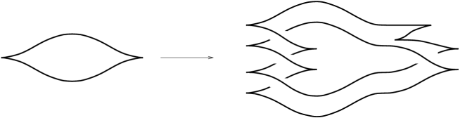
$K_{1}$$-1$$K_{2}$$-1$$K$$-5/3$

Figure 4. An example for the algorithm.

Remark 1.7.

In [2] the sequence of $(-1)$-surgeries replacing a contact $r$-surgery was defined iteratively, each surgery being performed along the Legendrian spine of the solid torus glued in when performing the preceding surgery. There are two ways to see that this is equivalent to performing successive surgeries along Legendrian push-offs: Assume $Y^{\prime}$ is obtained from $(Y,\xi)$ by contact $(-1)$-surgery along a Legendrian knot $K$, and write

$$Y^{\prime}=(Y\setminus\nu K)\cup S^{1}\times D^{2}$$

as before. In the handle picture of [2, Section 3], one can check that the belt sphere of the $2$-handle corresponding to this surgery is Legendrian isotopic in $Y^{\prime}$ to a Legendrian knot $K^{\prime}\subset Y\setminus\nu K\subset Y^{\prime}$ which, when regarded as a knot in $Y$, is a Legendrian push-off of $K$. Alternatively, the Legendrian push-off of a Legendrian knot $K$ is a knot Legendrian isotopic to $K$ and isotopic on $\partial(\nu K)$ to either of the dividing curves on that convex surface (cf. [1] for these concepts). The same is true for the spine of the glued in $S^{1}\times D^{2}$, and the gluing is defined by the matching of these dividing curves.

Contact $r$-surgery with $r>0$. Write $r=p/q$ with $p,q$ coprime positive integers. Choose a positive integer $k$ such that $q-kp<0$, and set $r^{\prime}=p/(q-kp)$. Let $K_{1},\ldots,K_{k}$ be $k$ successive Legendrian push-offs of a Legendrian knot $K$. Then contact $r$-surgery along $K$ is equivalent to contact $(+1)$-surgeries along $K$ and $K_{1},\ldots,K_{k-1}$, and a contact $r^{\prime}$-surgery along $K_{k}$.

2. Spin^c structures on 3- and 4-manifolds

$2$-plane fields and spin^c structures on $3$-manifolds

In the following we should like to describe surgery diagrams for contact structures on various 3-manifolds, including all overtwisted structures. Since, by [3], these latter contact structures (up to isotopy) are in one-to-one correspondence with oriented 2-plane fields (up to homotopy), we begin our discussion by a review of 2-plane fields on 3-manifolds, see [12] and cf. also the discussion in [11] and [16].

Let us fix a closed, oriented 3-manifold $Y$ and consider the space $\Xi(Y)$ of oriented 2-plane fields on $Y$. By considering the oriented normal unit vector field, we see that the elements of $\Xi(Y)$ are in one-to-one correspondence with the elements of the space of vector fields of unit length.

Definition 2.1.

Two nowhere vanishing vector fields $v_{1}$ and $v_{2}$ are said to be homologous if $v_{1}$ is homotopic to $v_{2}$ outside a ball $D^{3}\subset Y$ (through nowhere vanishing vector fields). An equivalence class of homologous vector fields is a spin^c structure on $Y$. The set of all spin^c structures is denoted by $Spin^{c}(Y)$.

Remark 2.2.

Traditionally, spin^c structures are defined as lifts of the orthonormal frame bundle of $Y$ to a principal bundle with structure group $Spin^{c}(3)=U(2)$. The equivalence with the definition given above was observed by Turaev [19].

Let $\mathbf{t}_{\xi}$ denote the spin^c structure induced by $\xi\in\Xi(Y)$ (by taking the oriented normal of the $2$-plane field); this $\mathbf{t}_{\xi}$ depends only on the homotopy class $[\xi]$ of $\xi$. The induced map $[\xi]\mapsto\mathbf{t}_{\xi}$ will be denoted by $p\colon\pi_{0}(\Xi(Y))\to Spin^{c}(Y)$; it is obviously surjective. It is easy to verify that if $p([\xi_{1}])=p([\xi_{2}])$ then we have equality of first Chern classes $c_{1}(\xi_{1})=c_{1}(\xi_{2})\in H^{2}(Y)$ (where we regard the oriented ${\mathbb{R}}^{2}$-bundles $\xi_{i}$, uniquely up to homotopy, as complex line bundles). Therefore we can define the first Chern class of a spin^c structure $\mathbf{t}\in Spin^{c}(Y)$. For the following standard fact cf. [19].

Proposition 2.3.

The second cohomology group $H^{2}(Y;{\mathbb{Z}})$ acts freely and transitively on $Spin^{c}(Y)$. If this action is denoted by $\mathbf{t}\otimes a$ for $\mathbf{t}\in Spin^{c}(Y)$ and $a\in H^{2}(Y;{\mathbb{Z}})$ then $c_{1}(\mathbf{t}\otimes a)=c_{1}(\mathbf{t})+2a$. In particular, if $H^{2}(Y;{\mathbb{Z}})$ has no $2$-torsion, then a spin^c structure $\mathbf{t}$ is uniquely specified by its first Chern class $c_{1}(\mathbf{t})$.

For $\mathbf{t}\in Spin^{c}(Y)$ the fibre $p^{-1}(\mathbf{t})$ can be easily identified with the homotopy classes of $2$-plane fields obtained by taking the connected sum of $(Y,\xi)$ (where $[\xi]\in p^{-1}(\mathbf{t}))$ with the elements of

$$\{(S^{3},\eta)\mid\eta{\mbox{ is an oriented $2$-plane field on }}S^{3}\}$$

(after pasting the $2$-plane fields together). In this way we get a transitive but not necessarily free ${{\mathbb{Z}}}$-action on that fibre.

For $\mathbf{t}\in Spin^{c}(Y)$ we denote the divisibility of the (well-defined) first Chern class $c_{1}(\mathbf{t})\in H^{2}(Y;{\mathbb{Z}})$ by $d(\mathbf{t})$ (which is set to zero if $c_{1}(\mathbf{t})$ is torsion). In the following lemma note that ${\mathbb{Z}}_{0}={\mathbb{Z}}$.

Lemma 2.4 ([12, Prop. 4.1]).

The fibre $p^{-1}(\mathbf{t})\subset\pi_{0}(\Xi(Y))$ admits a free and transitive ${\mathbb{Z}}_{d(\mathbf{t})}$-action. ∎

Therefore, for a spin^c structure whose first Chern class is torsion, the obstruction to homotopy of two $2$-plane fields both inducing that given spin^c structure can be captured by a single number. This obstruction (frequently called the 3-dimensional invariant $d_{3}$ of $\xi$) can be described as follows: Suppose that a compact almost complex 4-manifold $(X,J)$ is given such that $\partial X=Y$. (Recall that an almost complex structure on $X$ is a bundle homomorphism $J\colon TX\to TX$ with $J^{2}=-$id_TX.) The almost complex structure naturally induces a 2-plane field $\xi$ on $Y$ by taking the complex tangencies in $TY$, i.e., $\xi=TY\cap J(TY)$. Write $\sigma(X),\chi(X)$ for the signature and Euler characteristic of $X$, respectively.

Theorem 2.5 ([12, Thm. 4.16]).

For $c_{1}(\xi)$ a torsion class, the rational number

$$d_{3}(\xi)=\frac{1}{4}\bigl{(}c_{1}^{2}(X,J)-3\sigma(X)-2\chi(X)\bigr{)}$$

is an invariant of the homotopy type of the $2$-plane field $\xi$. Moreover, two $2$-plane fields $\xi_{1}$ and $\xi_{2}$ with $\mathbf{t}_{\xi_{1}}=\mathbf{t}_{\xi_{2}}$ and $c_{1}(\mathbf{t}_{\xi_{i}})=c_{1}(\xi_{i})$ a torsion class are homotopic if and only if $d_{3}(\xi_{1})=d_{3}(\xi_{2}).$ ∎

Remark 2.6.

It is fairly easy to see that for $Y=S^{3}$ the 3-dimensional invariant $d_{3}$ of a 2-plane field lies in ${\mathbb{Z}}+\frac{1}{2}$: for any characteristic vector, hence for $c_{1}(X,J)$ of an almost-complex structure, we have $c_{1}^{2}(X,J)\equiv\sigma(X)$ (mod 8) and $\frac{1}{2}(\sigma(X)+\chi(X))=\frac{1}{2}-b_{1}(X)+b^{+}_{2}(X)$. The 3-dimensional invariant $d_{3}$ of $(S^{3},\xi_{st})$ (as defined by Theorem 2.5) is $-\frac{1}{2}$, since we can regard $(S^{3},\xi_{st})$ as the boundary of the unit disc in ${\mathbb{C}}^{2}$.

Almost complex structures and spin^c structures on $4$-manifolds

Let $X$ be a compact 4-manifold, possibly with nonempty boundary $\partial X$. By a reasoning similar to the $3$-dimensional situation one can see that an almost complex structure defined on the complement of finitely many points of $X$ gives rise to a spin^c structure on $X$. (This is because both $S^{3}$ and $D^{4}$ admit unique spin^c structures.) It is fairly easy to see that two such almost complex structures induce the same spin^c structure if and only if they are homotopic on the 2-skeleton of $X$. This motivates the following definition:

Definition 2.7.

Two almost complex structures $J_{1},J_{2}$ defined on the complement of finitely many points in $X$ are homologous if there is a compact $1$-manifold $C\subset X$ containing the finitely many points where the $J_{i}$ are undefined such that $J_{1}$ is homotopic to $J_{2}$ on $X-C$ (through almost complex structures). An equivalence class of homologous almost complex structures is called a spin^c structure. The set of spin^c structures on $X$ is denoted by $Spin^{c}(X)$.

In analogy with the $3$-dimensional case, there is a well-defined notion of a first Chern class $c_{1}(\mathbf{s})$ for $\mathbf{s}\in Spin^{c}(X)$. The image of the map $c_{1}\colon Spin^{c}(X)\rightarrow H^{2}(X;{{\mathbb{Z}}})$ turns out to equal the set

$$\{c\in H^{2}(X;{\mathbb{Z}})\mid c\equiv w_{2}(X)\;\mbox{\rm mod}\;2\}$$

of characteristic elements. Once again, $H^{2}(X;{{\mathbb{Z}}})$ acts freely and transitively on $Spin^{c}(X)$; we denote this action by $(\mathbf{s},a)\mapsto\mathbf{s}\otimes a$. Again we have $c_{1}(\mathbf{s}\otimes a)=c_{1}(\mathbf{s})+2a$. Therefore, if $H^{2}(X;{{\mathbb{Z}}})$ has no $2$-torsion, for instance if $X$ is simply connected, then a spin^c structure $\mathbf{s}$ is uniquely determined by its first Chern class $c_{1}(\mathbf{s})$.

If $Y$ is a $3$-dimensional submanifold of $X$, then a spin^c structure on $X$ naturally induces a spin^c structure on $Y$ by taking the orthogonals of the complex tangencies in $TY$.

Homological data of $2$-handlebodies.

In our later arguments we shall make computations involving homology and cohomology classes on 2-handlebodies and on their boundaries. So let us assume that the 4-manifold $X$ is given by the framed link $\mathbb{L}=((K_{1},n_{1}),\ldots,(K_{t},n_{t}))\subset S^{3}$, i.e., we attach copies of $D^{2}\times D^{2}$ along $\partial D^{2}\times D^{2}$ to $D^{4}$ along $\nu K_{i}\subset\partial D^{4}=S^{3}$ with the specified framing $n_{i}$. (For more about such Kirby diagrams see [13]. Note that we only deal with the case when $X$ is decomposed into one 0-handle and a certain number $t$ of 2-handles.)

Obviously $\pi_{1}(X)=1$, and $H_{2}(X;{\mathbb{Z}})$ is generated by the fundamental classes $[\Sigma_{i}]$ of the surfaces $\Sigma_{i}$ we get by gluing a Seifert surface $F_{i}$ of $K_{i}$ to the core disc of the $i^{th}$ handle. The intersection form in this basis of $H_{2}(X;{\mathbb{Z}})$ is simply the linking matrix of $\mathbb{L}$, with the framing coefficients $n_{i}$ in the diagonal.

Let $N_{i}$ denote a small normal disc to $K_{i}$ in $S^{3}$ and $\mu_{i}=\partial N_{i}$. An orientation on the knot $K_{i}$ will give an orientation of $\Sigma_{i}$ (by requiring that the orientation of $K_{i}$ be the boundary orientation of the Seifert surface $F_{i}$). Together with the orientation of the ambient 3-manifold $S^{3}$, the orientation of $K_{i}$ will induce an orientation on $N_{i}$ as well. We can then give $\mu_{i}=\partial N_{i}$ the boundary orientation. In the knot diagrams below the orientation of $K_{i}$ will be denoted by a little arrow next to the diagram of the knot.

It is easy to see that the relative homology classes $[N_{i}]$ freely generate $H_{2}(X,\partial X;{\mathbb{Z}})$, while $H_{1}(\partial X;{\mathbb{Z}})$ is generated by the homology classes $[\mu_{i}]$ of the circles $\mu_{i}=\partial N_{i}$ ($i=1,\ldots,t$). The long exact sequence of the pair $(X,\partial X)$ reduces to

$$0\to H_{2}(\partial X;{\mathbb{Z}})\to H_{2}(X;{\mathbb{Z}})\stackrel{{\scriptstyle\varphi_{1}}}{{\longrightarrow}}H_{2}(X,\partial X;{\mathbb{Z}})\stackrel{{\scriptstyle\varphi_{2}}}{{\longrightarrow}}H_{1}(\partial X;{\mathbb{Z}})\to 0,$$

since the condition $\pi_{1}(X)=1$ implies

$$H_{1}(X;{\mathbb{Z}})=0=H^{1}(X;{\mathbb{Z}})\cong H_{3}(X,\partial X;{\mathbb{Z}}).$$

The maps $\varphi_{1}$ and $\varphi_{2}$ are easy to describe in the above bases: With $\ell k(K_{i},K_{j})$ denoting the linking number of $K_{i}$ and $K_{j}$ for $i\neq j$ and $\ell k(K_{i},K_{i})=n_{i}$ we have

$$\varphi_{1}([\Sigma_{i}])=\sum_{j=1}^{t}\ell k(K_{i},K_{j})[N_{j}];$$

furthermore

$$\varphi_{2}([N_{i}])=[\mu_{i}].$$

(For details of the argument see [13].) For a cohomology class $c\in H^{2}(X;{\mathbb{Z}})$ denote by $c(\Sigma_{i})=\langle c,[\Sigma_{i}]\rangle\in{\mathbb{Z}}$ its evaluation on $\Sigma_{i}$. Then the Poincaré dual $PD(c)\in H_{2}(X,\partial X;{\mathbb{Z}})$ is equal to $\sum_{i=1}^{t}c(\Sigma_{i})[N_{i}]$. The image $\varphi_{2}(PD(c))$ gives a description of $PD(c|_{\partial X})$ in terms of the 1-homologies $[\mu_{i}]$. Exactness of the sequence implies that the relations among the $[\mu_{i}]$ are simply given by the expressions $\varphi_{1}([\Sigma_{i}])$ with $[N_{i}]$ substituted by $[\mu_{i}]$. These relations help to simplify $PD(c|_{\partial X})$. If that class is a torsion element then for appropriate $n\in{\mathbb{N}}$ the class $PD(n\cdot c)$ maps to zero under $\varphi_{2}$, hence it is the image of a class $C\in H_{2}(X;{\mathbb{Z}})$ under $\varphi_{1}$. In that case we can compute $c^{2}$ as $c^{2}=C^{2}/n^{2}$.

3. Computation of homotopy invariants of contact structures

From a surgery presentation of $(Y,\xi)$ we now wish to determine some homotopy invariants of $\xi$. The surgery diagram can be considered as a Kirby diagram for a 4-manifold $X$ with boundary $Y$. Consider $(S^{3},\xi_{st})$ as the boundary of the standard disc $D^{4}\subset{\mathbb{C}}^{2}$, equipped with its standard (almost) complex structure.

Proposition 3.1 ([4], [12, Prop. 2.3]).

If a $2$-handle $H$ is attached along a Legendrian knot $K\subset(S^{3},\xi_{st})$ with framing $(-1)$ (i.e. one left twist added to the contact framing) then the above standard complex structure extends as an (almost) complex structure $J$ to $D^{4}\cup H$ inducing the surgered contact structure on the boundary. Moreover, $c_{1}(D^{4}\cup H,J)$ evaluates on the homology class given by $K$ (in the sense of the previous section) as ${\rm{rot}}(K)$.∎

Remark 3.2.

In fact, Eliashberg [4] showed that the Stein structure of $D^{4}$ extends as a Stein structure to $D^{4}\cup H$, cf. [10].

We now want to study the related question for contact $(+1)$-surgeries. Thus, let $X=D^{4}\cup H$ be the handlebody corresponding to a contact $(+1)$-surgery on a Legendrian knot $K\subset(S^{3},\xi_{st})=\partial D^{4}$. The contact structure $\xi$ on $\partial X$ determined by the surgery defines an almost complex structure $J$ (on $X$) along $\partial X$, unique up to homotopy: require, firstly, $\xi$ to be $J$-invariant (and the orientation of $\xi$ induced by $J$ to coincide with the given one) and, secondly, $J$ to map the outward normal along $\partial X$ to a vector positively transverse to $\xi$.

That $J$ extends to the complement of a $4$-disc $D_{H}\subset\mbox{\rm int}(H)\subset X$, for there is no obstruction to extending $J$ over the cocore $2$-disc of the $2$-handle, and $X-D_{H}$ deformation retracts onto the union of $\partial X$ and that cocore disc. In particular, there is a class $c\in H^{2}(X;{{\mathbb{Z}}})$ that restricts to $c_{1}(\xi)=c_{1}(J)$ on $\partial X$, and whose mod $2$ reduction equals $w_{2}(X)$; the existence of such a class (which conversely implies the existence of $J$ on $X-D_{H}$) can also be shown by a purely homological argument.

Let $\xi_{H}$ be the plane field on $\partial D_{H}=S^{3}$ induced by $J$, where $\partial D_{H}$ is given the orientation as boundary of $D_{H}\subset X$ rather than the boundary orientation of $\partial(X-D_{H})$. By [12], cf. [13, Thm. 11.3.4] and the discussion preceding it, there is an almost complex manifold $(W,J_{W})$ with $\partial W=S^{3}$ such that $J_{W}$ induces the plane field $\xi_{H}$ on the boundary. With the help of $W$ one can compute the invariant $d_{3}(\xi_{H})$. Moreover, by the proof of that same quoted theorem the $d_{3}$-invariant behaves additively in the sense that

$$d_{3}(\xi) = \frac{1}{4}\bigl{(}c_{1}^{2}(X-D_{H},J)-3\sigma(X-D_{H})-2\chi(X-D_{H})\bigr{)}+d_{3}(\xi_{H})$$

$$= \frac{1}{4}\bigl{(}c^{2}-3\sigma(X)-2\chi(X)\bigr{)}+d_{3}(\xi_{H})+\frac{1}{2}.$$

Remark 3.3.

As part of the following proposition we shall see that $d_{3}(\xi_{H})=1/2$. This equals the $d_{3}$-invariant of the standard contact structure on $S^{3}$, regarded as the boundary of ${{\mathbb{C}}}P^{2}-D^{4}$ (i.e. with the opposite of the usual orientation, which causes the sign change of the $d_{3}$-invariant, cf. [13, Thm. 11.3.4] again). Thus an equivalent way of phrasing the result $d_{3}(\xi_{H})=1/2$ is that the almost complex structure defined near $\partial X$ extends over $X\#{{\mathbb{C}}}P^{2}$, coinciding with the standard structure near the $2$-skeleton of ${{\mathbb{C}}}P^{2}$. (See also Section 5 below.)

On the other hand, recall from [2] that contact $(+1)$-surgery can be regarded as a symplectic handlebody surgery on the concave end of a symplectic cobordism. In particular, we may regard $(S^{3},\xi_{st})$ (with reversed orientation) as the concave boundary of ${\mathbb{C}}P^{2}-D^{4}$ with its standard Kähler structure, and contact $(+1)$-surgery along $K$ corresponds to adding a symplectic $2$-handle to ${\mathbb{C}}P^{2}-D^{4}$ along its boundary. This implies that the contact structure on $\partial X$ with reversed orientation is induced from an almost complex structure on $\overline{X}\#{{\mathbb{C}}}P^{2}$, again coinciding with the standard structure near the $2$-skeleton of ${{\mathbb{C}}}P^{2}$. (Here $\overline{X}$ denotes $X$ with reversed orientation.)

Thus, we can glue $X\#{{\mathbb{C}}}P^{2}$ and $\overline{X}\#{{\mathbb{C}}}P^{2}$ along their common boundary (with opposite orientations) to obtain an almost complex manifold

$${{\mathbb{C}}}P^{2}\#X\cup\overline{X}\#{{\mathbb{C}}}P^{2}={{\mathbb{C}}}P^{2}\#DX\#{{\mathbb{C}}}P^{2},$$

where $DX$ denotes the double of $X$, which in the present situation is diffeomorphic to $S^{2}\times S^{2}$ or ${{\mathbb{C}}}P^{2}\#\overline{{{\mathbb{C}}}P^{2}}$, cf. [13, Cor. 5.1.6]. Indeed, a homological calculation similar to the following proof shows that ${{\mathbb{C}}}P^{2}\#DX\#{{\mathbb{C}}}P^{2}$ admits an almost complex structure, standard near the $2$-skeleta of the ${{\mathbb{C}}}P^{2}$-summands, which splits in the way described.

If $X$ is a handlebody corresponding to $n$ contact $(+1)$-surgeries, then the contact manifold $\partial X$ is boundary of the almost complex manifold $X\#n{{\mathbb{C}}}P^{2}$; with reversed orientation it is the boundary of $\overline{X}\#{{\mathbb{C}}}P^{2}$. Again one checks that $n{{\mathbb{C}}}P^{2}\#DX\#{{\mathbb{C}}}P^{2}$ admits an appropriate almost complex structure. ($DX$ is diffeomorphic to $nS^{2}\times S^{2}$ or $n{{\mathbb{C}}}P^{2}\#n\overline{{{\mathbb{C}}}P^{2}}$, cf.  [13, Cor. 5.1.6].)

Proposition 3.4.

Let $K\subset(S^{3},\xi_{st})$ be a Legendrian knot with $\mbox{\rm tb}(K)\neq 0$. If the handlebody $X$ is obtained by attaching a $2$-handle $H$ to $D^{4}$ along $K$ with framing $(+1)$ (one right twist added to the contact framing), then the almost complex structure defined near $\partial X$ extends over $X-D_{H}$, in the previously introduced notation, such that $d_{3}(\xi_{H})=1/2$. Moreover, the corresponding class $c\in H^{2}(X;{{\mathbb{Z}}})$ evaluates on the homology class given by $K$ as $\mbox{\rm rot}(K)$.

Proof.

Consider Legendrian push-offs $K_{1},\ldots,K_{n},K_{1}^{\prime},\ldots,K_{n}^{\prime}$ of $K$ (it would be enough to study the cases $n=1$ or $2$). Perform contact $(+1)$-surgeries on $K_{1},\ldots,K_{n}$ and contact $(-1)$-surgeries on $K_{1}^{\prime},\ldots,K_{n}^{\prime}$. By Lemma 1.1 the resulting manifold is $(S^{3},\xi_{st})$.

Let

$$\Sigma_{1},\ldots,\Sigma_{n},\Sigma_{1}^{\prime},\ldots,\Sigma_{n}^{\prime}$$

be the corresponding surfaces in

$$X=X_{n}=D^{4}\cup H_{1}\cup\ldots\cup H_{n}\cup H_{1}^{\prime}\cup\ldots\cup H_{n}^{\prime}$$

in the notation of the preceding section. Write $c=c_{(n)}\in H^{2}(X_{n};{\mathbb{Z}})$ for the class defined by the almost complex structure on $X$ with discs $D_{H_{1}},\ldots,D_{H_{n}}$ removed. By Proposition 3.1 we have $c(\Sigma_{i}^{\prime})=\mbox{\rm rot}(K)$, $i=1,\ldots,n$. Set $k=c(\Sigma_{i})$. Then, again by the preceding section (and in the notation used there),

$$PD(c)=k\sum_{i=1}^{n}[N_{i}]+\mbox{\rm rot}(K)\sum_{i=1}^{n}[N_{i}^{\prime}].$$

This can be written as $PD(c)=\varphi_{1}(C)$ with a unique class $C\in H_{2}(X;{\mathbb{Z}})$ (since $H_{1}(\partial X)=H_{2}(\partial X)=0$). We have

$$\varphi_{1}([\Sigma_{i}])=\mbox{\rm tb}(K)\sum_{j=1}^{n}\bigl{(}[N_{j}]+[N_{j}^{\prime}]\bigr{)}+[N_{i}]$$

and

$$\varphi_{1}([\Sigma_{i}^{\prime}])=\mbox{\rm tb}(K)\sum_{j=1}^{n}\bigl{(}[N_{j}]+[N_{j}^{\prime}]\bigr{)}-[N_{i}^{\prime}].$$

Write

$$C=\sum_{i=1}^{n}\bigl{(}a_{i}[\Sigma_{i}]+a_{i}^{\prime}[\Sigma_{i}^{\prime}]\bigr{)}.$$

Then the coefficients $a_{i},a_{i}^{\prime}$ are found as solutions of the linear equation

$$M_{\mbox{\scriptsize\rm tb}(K)}\left(\begin{array}[]{c}a_{1}\\ \vdots\\ a_{n}\\ a_{1}^{\prime}\\ \vdots\\ a_{n}^{\prime}\end{array}\right)=\left(\begin{array}[]{c}k\\ \vdots\\ k\\ \mbox{\rm rot}(K)\\ \vdots\\ \mbox{\rm rot}(K)\end{array}\right),$$

where $M_{\mbox{\scriptsize\rm tb}(K)}$ is the matrix

$$M_{\mbox{\scriptsize\rm tb}(K)}=\mbox{\rm tb}(K)E_{2n}+\left(\begin{array}[]{cc}I_{n}&0\\ 0&-I_{n}\end{array}\right),$$

with $E_{2n}$ the $(2n\times 2n)$-matrix having all entries equal to $1$, and $I_{n}$ the $(n\times n)$ unit matrix.

It follows that

$$a_{1}=\cdots=a_{n}=k-n\bigl{(}k-\mbox{\rm rot}(K)\bigr{)}\mbox{\rm tb}(K)$$

and

$$a_{1}^{\prime}=\cdots=a_{n}^{\prime}=-\mbox{\rm rot}(K)+n\bigl{(}k-\mbox{\rm rot}(K)\bigr{)}\mbox{\rm tb}(K),$$

whence

$$c^{2}\;=\;C^{2} = \bigl{(}a_{1},\ldots,a_{n},a_{1}^{\prime},\ldots,a_{n}^{\prime}\bigr{)}M_{\mbox{\scriptsize\rm tb}(K)}\left(\begin{array}[]{c}a_{1}\\ \vdots\\ a_{n}\\ a_{1}^{\prime}\\ \vdots\\ a_{n}^{\prime}\end{array}\right)$$

$$= \bigl{(}a_{1},\ldots,a_{n},a_{1}^{\prime},\ldots,a_{n}^{\prime}\bigr{)}\left(\begin{array}[]{c}k\\ \vdots\\ k\\ \mbox{\rm rot}(K)\\ \vdots\\ \mbox{\rm rot}(K)\end{array}\right)$$

$$= n\bigl{(}k^{2}-\mbox{\rm rot}^{2}(K)\bigr{)}-n^{2}\mbox{\rm tb}(K)\bigl{(}k-\mbox{\rm rot}(K)\bigr{)}^{2}.$$

The signature of $M_{\mbox{\scriptsize\rm tb}(K)}$ (which is the same as the signature of $X$) is equal to zero (this follows from the fact that $M_{\mbox{\scriptsize\rm tb}(K)}$ remains nonsingular if $\mbox{\rm tb}(K)$ is replaced by any real parameter). The Euler characteristic of $X$ is $1+2n$.

From the discussion preceding the present proposition we deduce

$$-\frac{1}{2}=d_{3}(S^{3},\xi_{st})=$$

$$=\frac{1}{4}\bigl{(}c_{1}^{2}(X-\bigcup_{i}D_{H_{i}},J)-3\sigma(X)-2\chi(X)\bigr{)}+n\bigl{(}d_{3}(\xi_{H})+\frac{1}{2}\bigr{)}$$

$$=\frac{1}{4}\bigl{[}n\bigr{(}k^{2}-\mbox{\rm rot}^{2}(K)\bigr{)}-n^{2}\mbox{\rm tb}(K)\bigl{(}k-\mbox{\rm rot}(K)\bigr{)}^{2}\bigr{]}+$$

$$\;\;\;\;\;\;\;\mbox{}+n\bigl{(}d_{3}(\xi_{H})-\frac{1}{2}\bigr{)}-\frac{1}{2}.$$

This is true for any $n\in{\mathbb{N}}$, from which we conclude, for $\mbox{\rm tb}(K)\neq 0$, that $k=\mbox{\rm rot}(K)$ and $d_{3}(\xi_{H})=1/2$. ∎

Remark 3.5.

The result $d_{3}(\xi_{H})=1/2$ remains true even if $\mbox{\rm tb}(K)=0$. This can be seen from the description of contact $(+1)$-surgery in [2] as a symplectic handlebody surgery on the concave end of a symplectic cobordism. Indeed, this description provides a unique model for contact $(+1)$-surgery, so that the obstruction for extending the almost complex structure over the handle is independent of $\mbox{\rm tb}(K)$.

In the case $\mbox{\rm tb}(K)=0$ the above argument only yields $k=\pm{\rm{rot}}(K)$. The quickest way to see that $k={\rm{rot}}(K)$ in this case as well is the following: Since, as just remarked, contact $(+1)$-surgery also admits a handlebody description, one can mimic the argument of [12, Prop. 2.3], where the corresponding result was shown for contact $(-1)$-surgeries. Checking all the relevant signs might be tedious, but again the argument shows that $k$ does not depend on $\mbox{\rm tb}(K)$, so our result $k=\mbox{\rm rot}(K)$ for $\mbox{\rm tb}(K)\neq 0$ in fact also holds in the case $\mbox{\rm tb}(K)=0$.

Since we shall not use the result for ${\rm{tb}}(K)=0$ in our subsequent arguments, we defer an explicit discussion of these issues to Section 5.

Corollary 3.6.

Suppose that $(Y,\xi)=\partial X$, with $c_{1}(\xi)$ torsion, is given by contact $(\pm 1)$-surgery on a Legendrian link ${\mathbb{L}}\subset(S^{3},\xi_{st})$ with $\mbox{\rm tb}(K)\neq 0$ for each $K\subset{\mathbb{L}}$ on which we perform contact $(+1)$-surgery. Then

$$d_{3}(\xi)=\frac{1}{4}\bigl{(}c^{2}-3\sigma(X)-2\chi(X)\bigr{)}+q,$$

where $q$ denotes the number of components in ${\mathbb{L}}$ on which we perform $(+1)$-surgery, and $c\in H^{2}(X;{\mathbb{Z}})$ is the cohomology class determined by $c(\Sigma_{K})={\rm{rot}}(K)$ for each $K\subset\mathbb{L}$. Here $[\Sigma_{K}]$ is the homology class in $H_{2}(X)$ determined by $K\subset S^{3}$ (i.e. Seifert surface of $K$ glued with core disc of corresponding handle).

Proof.

The contact manifold $(Y,\xi)$ is the boundary of the almost complex manifold $X\#q{\mathbb{C}}P^{2}$ (such that $\xi$ is given by the complex tangencies in $Y=\partial X$), with first Chern class

$$c_{1}=c+(3,\ldots,3)\in H^{2}(X;{\mathbb{Z}})\oplus qH^{2}({\mathbb{C}}P^{2};{\mathbb{Z}}),$$

which satisfies $c_{1}^{2}=c^{2}+9q$.

Moreover,

$$\sigma(X\#q{\mathbb{C}}P^{2})=\sigma(X)+q$$

and

$$\chi(X\#q{\mathbb{C}}P^{2})=\chi(X)+q.$$

Hence

$$d_{3}(\xi) = \frac{1}{4}\bigl{(}c^{2}+9q-3(\sigma(X)+q)-2(\chi(X)+q)\bigr{)}$$

$$= \frac{1}{4}\bigl{(}c^{2}-3\sigma(X)-2\chi(X)\bigr{)}+q.$$

∎

4. Surgery diagrams for overtwisted contact $3$-manifolds

Our next goal is to draw surgery diagrams for all overtwisted contact structures on a given 3-manifold $Y$. Recall from [3] that overtwisted contact structures (up to isotopy) are in one-to-one correspondence with elements of $\pi_{0}(\Xi(Y))$. Therefore, in order to find all the necessary diagrams, we need to find, for each spin^c structure on $Y$, a surgery diagram for a contact structure inducing that spin^c structure, and diagrams for all overtwisted contact structures on $S^{3}$. By taking connected sums of these structures – which is reflected simply as disjoint union in the diagrams – we get all the pictures we wanted. First we show how to draw surgery diagrams for all contact structures on $S^{3}$. Then we do the same for $S^{1}\times S^{2}$, and finally we turn to the general case.

Notice also that if $(Y,\xi)$ is a contact structure with $c_{1}(\mathbf{t}_{\xi})$ torsion and $(S^{3},\xi_{i})$ is an arbitrary contact structure, then

$$d_{3}(Y,\xi\#\xi_{i})=d_{3}(Y,\xi)+d_{3}(S^{3},\xi_{i})+\frac{1}{2}.$$

This follows from the fact that under the boundary connected sum $X\natural X^{\prime}$ of $4$-manifolds $X,X^{\prime}$, the signature $\sigma$ and the number $c^{2}$ behave additively, whereas

$$\chi(X\natural X^{\prime})=\chi(X)+\chi(X^{\prime})-1.$$

Contact structures on $S^{3}$

By Eliashberg’s classification [3], [5] we know that $S^{3}$ admits a unique tight contact structure $\xi_{st}$ (which can be represented by the empty diagram in $(S^{3},\xi_{st})$), and a unique overtwisted one (up to isotopy) in each homotopy class of 2-plane fields. Obviously, all these structures have zero first Chern class; the overtwisted ones can be distinguished by their 3-dimensional invariant $d_{3}$.

Lemma 4.1.

The surgery diagram of Figure 5(a) gives a contact structure $\xi_{1}$ on $S^{3}$ with $d_{3}(\xi_{1})=\frac{1}{2}$. The surgery diagram of Figure 6(a) gives a contact structure $\xi_{-1}$ on $S^{3}$ with $d_{3}(\xi_{-1})=-\frac{3}{2}$.

$+1$$-1$$\cong$$(a)$$(b)$

Figure 5. Contact structure $\xi_{1}$ on $S^{3}$ with $d_{3}(\xi_{1})=1/2$.

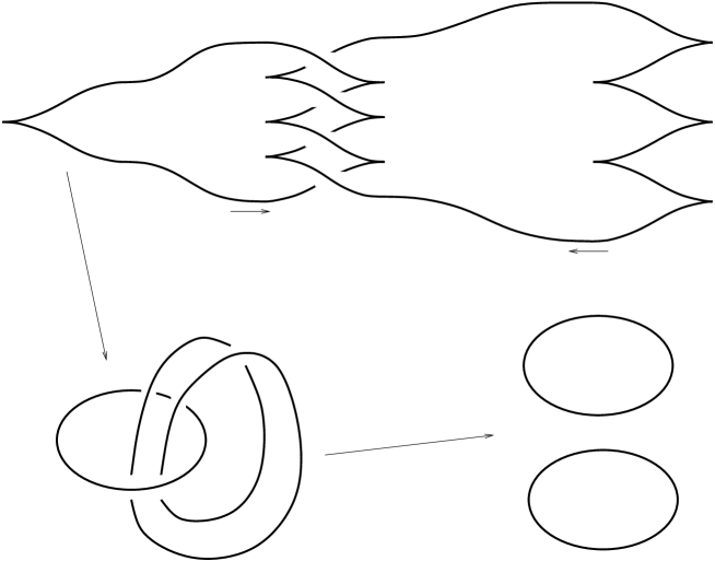
$-1$$-1$$\cong$$K_{1}$$-5$$-1$$K_{2}$$+1$$K_{1}$$-1$$K_{2}$$\cong$$(a)$$(b)$

Figure 6. Contact structure $\xi_{-1}$ on $S^{3}$ with $d_{3}(\xi_{-1})=-3/2$.

Proof.

By turning the diagrams into smooth surgery diagrams (i.e., disregarding the Legendrian position of the surgery curves and thus the induced contact structure on the result) and reading the framings not relative to the contact framing, but relative to the framings induced by the Seifert surfaces in $S^{3}$, we see that topologically the two surgeries yield $S^{3}$. The equivalence between the surgery descriptions in Figure 6(b) (even as Kirby diagrams of a $4$-manifold) is given by a handle slide; cf. [13, p. 150].

Here is the computation of the $d_{3}$-invariants (with notation as above):

Recall from [12], [13] that for a Legendrian knot $K$, represented by its front projection, we have

$$\mbox{\rm tb}(K)=\mbox{\rm writhe}(K)-\frac{1}{2}\#(\mbox{\rm cusps})$$

and

$$\mbox{\rm rot}(K)=\frac{1}{2}(\#(\mbox{\rm down-cusps})-\#(\mbox{\rm up-cusps})).$$

Thus, in the first case we have, with the indicated orientation of the Legendrian knot $K$, that $\mbox{\rm rot}(K)=1$. Hence

$$PD(c)=c(\Sigma)[N]=\mbox{\rm rot}(K)[N]=[N].$$

Since the topological framing of $K$ (i.e. the framing relative to the surface framing) is $k=-1$, we have $\varphi_{1}([\Sigma])=-[N]$. Therefore $C=-[\Sigma]$ and $c^{2}=C^{2}=k=-1$. Moreover, the corresponding handlebody $X=D^{4}\cup H$ has $\sigma(X)=\mbox{sign}(k)=-1$ and $\chi(X)=2$. Thus, by Corollary 3.6,

$$d_{3}(\xi_{1})=\frac{1}{4}(-1+3-4)+1=\frac{1}{2}.$$

In the second case, again with the indicated orientations, we have

$$\mbox{\rm tb}(K_{1})=-4,\;\;\mbox{\rm rot}(K_{1})=1,\;\;\mbox{\rm tb}(K_{2})=-2,\;\;\mbox{\rm rot}(K_{2})=-1.$$

Furthermore, the linking number $\ell k(K_{1},K_{2})$ equals $-2$, so the linking matrix, which describes the homomorphism $\varphi_{1}$, is $\left(\begin{array}[]{rr}-5&-2\\ -2&-1\end{array}\right)$. With

$$PD(c)=\mbox{\rm rot}(K_{1})[N_{1}]+\mbox{\rm rot}(K_{2})[N_{2}]=[N_{1}]-[N_{2}]$$

we find that the solution of $\varphi_{1}(C)=PD(c)$ is $C=-3[\Sigma_{1}]+7[\Sigma_{2}]$. Thus

$$c^{2}=C^{2}=(-3,7)\left(\begin{array}[]{rr}-5&-2\\ -2&-1\end{array}\right)\left(\begin{array}[]{c}-3\\ 7\end{array}\right)=-10.$$

Moreover, the corresponding handlebody $X=D^{4}\cup H_{1}\cup H_{2}$ has $\chi(X)=3$ and $\sigma(X)=-2$ (which is obvious from the smooth surgery description). We conclude

$$d_{3}(\xi_{-1})=\frac{1}{4}(-10+6-6)+1=-\frac{3}{2}.\qed$$

Using the connected sum operation on the two basic contact structures $\xi_{1}$ and $\xi_{-1}$, we can now draw diagrams for all overtwisted contact structures $\xi_{i}$ on $S^{3}$ with $d_{3}(\xi_{i})=i-1/2$ ($i\in{\mathbb{Z}})$. Of course, this procedure will not necessarily provide the most “economic ” surgery diagram of $\xi_{i}$.

Here is a brief sketch of an alternative construction: Let $K_{1}$ be a Legendrian knot in $(S^{3},\xi_{st})$. Let $K_{2}$ be the Legendrian knot obtained from a Legendrian push-off of $K_{1}$ by adding two zigzags to its front projection, and perform contact $(+1)$-surgery on both knots. Topologically, contact $(+1)$-surgery on $K_{2}$ is the same as contact $(-1)$-surgery along a Legendrian push-off of $K_{1}$, so the resulting manifold is again $S^{3}$ by Lemma 1.1. Write $\xi$ for the contact structure on $S^{3}$ obtained via that surgery.

Equip $K_{1}$ with an orientation. By a computation as in the proof of the preceding lemma, one finds that if $K_{2}$ is obtained from a Legendrian push-off of $K_{1}$ by adding two down-zigzags to its front projection, then $d_{3}(\xi)=-\mbox{\rm tb}(K_{1})-\mbox{\rm rot}(K_{1})-1/2$.

Any odd (but no even) integer can be realised as $\mbox{\rm tb}(K_{1})+\mbox{\rm rot}(K_{1})$ for a suitable Legendrian knot $K_{1}$. We leave it as an exercise to the reader to construct such $K_{1}$ (see the examples in [12] and [9]); that even integers are excluded follows from [6, Prop. 2.3.1]. Therefore, any overtwisted contact structure on $S^{3}$ can be obtained by contact $(+1)$-surgeries on either two or three Legendrian knots (to realise $d_{3}=2m-1/2$, $m\in{\mathbb{Z}}$, construct a contact structure $\xi$ on $S^{3}$ with $d_{3}(\xi)=(2m-1)-1/2$ by two $(+1)$-surgeries as just described, then take the connected sum with $(S^{3},\xi_{1})$).

Contact structures on $S^{1}\times S^{2}$

According to a folklore theorem of Eliashberg, $S^{1}\times S^{2}$ admits a unique tight contact structure (for a sketch proof see Exercise 6.10 in [7]).

Lemma 4.2.

Contact $(+1)$-surgery on the Legendrian unknot (see Figure 7) yields the tight contact structure on $S^{1}\times S^{2}$.

$+1$

Figure 7. Legendrian unknot producing tight $S^{1}\times S^{2}$.

Proof.

The Legendrian unknot shown in Figure 7 has Thurston-Bennequin invariant $-1$, thus contact $(+1)$-surgery corresponds to a topological $0$-surgery, which produces the manifold $S^{1}\times S^{2}$.

For the contact-geometric part of the proof we use the language of convex surfaces and dividing curves; for a brief introduction see [7]. By [15, Thm. 8.2] and [14, Prop. 4.3], for any $k\in{\mathbb{Z}}$ there is a unique tight contact structure on $S^{1}\times D^{2}$ with a fixed convex boundary with dividing set consisting of two curves of slope $1/k$, where the meridian corresponds to slope zero and the longitude $S^{1}\times\{p\}$, $p\in\partial D^{2}$, to slope $\infty$. Notice that different values of $k$ simply correspond to a different choice of longitude. It therefore suffices to show that both the standard tight contact structure on $S^{1}\times S^{2}$ and the contact structure obtained by the described surgery can be split along an embedded convex $T^{2}$ with dividing set as described.

The standard tight contact structure on $S^{1}\times S^{2}\subset S^{1}\times{\mathbb{R}}^{3}$ is given, in obvious notation, by

$$\alpha:=x\,d\theta+y\,dz-z\,dy=0.$$

Embed $T^{2}$ as follows:

$$\begin{array}[]{rcl}T^{2}&\longrightarrow&S^{1}\times S^{2}\\ (\theta,\varphi)&\longmapsto&(\theta,f(\varphi),\sqrt{1-f^{2}(\varphi)}\cos\varphi,\sqrt{1-f^{2}(\varphi)}\sin\varphi)\end{array}$$

with $f(\varphi)=\varepsilon\sin\varphi$ for some $\varepsilon\in(0,1)$. The tangent spaces of this embedded $T^{2}$ are spanned by $\partial_{\theta}$ and

$$v=(0,f^{\prime},-\frac{ff^{\prime}}{\sqrt{1-f^{2}}}\cos\varphi-\sqrt{1-f^{2}}\sin\varphi,-\frac{ff^{\prime}}{\sqrt{1-f^{2}}}\sin\varphi+\sqrt{1-f^{2}}\cos\varphi).$$

From $\alpha(\partial_{\theta})=f$ and $\alpha(v)=1-f^{2}$ we conclude that the characteristic foliation on $T^{2}$ is given by ${\displaystyle\partial_{\theta}-\frac{f}{1-f^{2}}\partial_{\varphi}}$, which admits the dividing curves $\{\varphi=\pi/2\}$ and $\{\varphi=3\pi/2\}$. This means that $T^{2}$ is a convex torus with dividing set consisting of two longitudes, as desired.

Now to the same question for the contact structure on $S^{1}\times S^{2}$ obtained via the indicated surgery. First of all, we recall that in the unique local contact geometric model for the tubular neighbourhood of a Legendrian knot, the boundary of that neighbourhood is a convex torus with dividing set consisting of two copies of the longitude determined by the contact framing, cf. [2]. Write $K$ for the Legendrian knot of Figure 7 and $\nu K$ for a (closed) tubular neighbourhood. Further, we denote the meridian of $\partial(\nu K)$ by $\mu$, and by $\lambda$ the longitude determined by $\ell k(\lambda,K)=0$.

Then $S^{3}-\mbox{\rm int}(\nu K)$ is a solid torus with meridian $\overline{\mu}=\lambda$ and a longitude $\overline{\lambda}=\mu$. Since $\mbox{\rm tb}(K)=-1$, the longitude $\lambda_{c}$ determined by the contact framing is

$$\lambda_{c}=\lambda-\mu=\overline{\mu}-\overline{\lambda},$$

which is a longitude of $S^{3}-\mbox{\rm int}(\nu K)$, so the tight contact structure on that piece has a convex boundary of the kind described above.

The surgered manifold ($(+1)$-surgery with respect to the framing given by $\lambda_{c}$) is given by

$$(S^{3}-\nu K)\cup N_{0},$$

where $N_{0}$ is a solid torus, with meridian $\mu_{0}$ and longitude $\lambda_{0}$ of $\partial N_{0}$ being glued to $\partial(\nu K)$ by

$$\mu_{0}\longmapsto-\lambda_{c}-\mu=-\lambda,\;\;\;\lambda_{0}\longmapsto\mu.$$

Observe that the curve $-\mu_{0}-\lambda_{0}$ is glued to a dividing curve $\lambda_{c}=\lambda-\mu$. So the extension of the contact structure over $N_{0}$ in the process of contact surgery is given by the unique tight contact structure with convex boundary having two copies of the longitude $-\mu_{0}-\lambda_{0}$ as dividing set. This concludes the proof. ∎

Remark 4.3.

An alternative proof of this lemma, deducing tightness from the non-vanishing of the corresponding Heegaard-Floer invariant, is given in [18, Lemma 4].

In order to have a diagram for each overtwisted contact structure on $S^{1}\times S^{2}$, we first have to find a diagram for contact structures representing each spin^c structure, and then form the connected sum of these with the contact structures found in the previous subsection for $S^{3}$. Notice that since $H^{2}(S^{1}\times S^{2};{\mathbb{Z}})\cong{\mathbb{Z}}$ has no 2-torsion, a spin^c structure is uniquely characterised by its first Chern class. So the problem reduces to finding a contact structure $\xi_{k}$ on $S^{1}\times S^{2}$ with $c_{1}(\xi_{k})=2k$ for all $k\in{\mathbb{Z}}$. (Recall that the first Chern class of a 2-plane field is always an even class.) First we inductively define the Legendrian knot $K_{k}$ by Figure 8.

$-1$$-1$$-1$$-1$$k-1$$k-1$$=$and$=$$1$$k-2$where

Figure 8. The Legendrian knot $K_{k}$.

Lemma 4.4.

For the oriented Legendrian knot $K_{k}$ defined by Figure 8, with $k\geq 2$, we have rot$(K_{k})=k-2$ and ${\rm{tb}}(K_{k})=1-k^{2}$.

Proof.

Recall from the proof of Lemma 4.1 the formulae for computing tb and rot from the front projection. Denote the contribution of the box to tb and rot by $t_{k-1}$ and $r_{k-1}$, respectively. Then by counting the cusps and crossings outside the box we see

$$\mbox{\rm tb}(K_{k})=t_{k-1}-(k-1)-\frac{1}{2}(k+1)=t_{k-1}-\frac{3}{2}k+\frac{1}{2}$$

and

$$\mbox{\rm rot}(K_{k})=r_{k-1}+\frac{1}{2}(1-k).$$

From the inductive definition of the box we have the recursive formulae

$$t_{1}=-\frac{1}{2},\;\;t_{k-1}=t_{k-2}-2(k-2)-\frac{3}{2}$$

and

$$r_{1}=\frac{1}{2},\;\;r_{k-1}=r_{k-2}+\frac{3}{2},$$

from which one finds

$$t_{k-1}=\frac{1}{2}-k^{2}+\frac{3}{2}k,\;\;\;r_{k-1}=-\frac{5}{2}+\frac{3}{2}k.$$

Substituting this into the expressions for tb and rot we obtain the claimed result. ∎

In the following proposition and its proof we use again the notation of Section 2; in particular, $\mu_{i}$ denotes a meridian of $K_{i}$.

Proposition 4.5.

For $k\geq 2$ the surgery diagram of Figure 9 defines a contact structure $\xi_{k}$ on $S^{1}\times S^{2}$ with $c_{1}(\xi_{k})=(2k-2)PD^{-1}([\mu_{2}])$. Here $[\mu_{2}]$ is a generator of $H_{1}(S^{1}\times S^{2};{\mathbb{Z}})\cong{\mathbb{Z}}$.

Here, by slight abuse of notation, $K_{2}$ denotes the Legendrian knot $K_{k}$ considered previously.

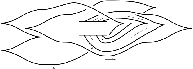
$-1$$k-1$$K_{2}$$K_{1}$$-1$$+1$

Figure 9. Surgery diagram of contact structure on $S^{1}\times S^{2}$.

Proof.

First of all, we need to check that the topological result of the described surgeries is $S^{1}\times S^{2}$. For that, we observe that the surgery diagram of Figure 9 is topologically equivalent to that of Figure 10, where the indicated framings are now relative to the surface framings in $S^{3}$. Blowing down the $(-1)$-framed unknot $K_{1}$ (see [13, p. 150]) adds a $(+1)$-twist to the $k$ strands of $K_{2}$ running through it (i.e. cancels the $(-1)$-box) and adds ${\ell k}(K_{1},K_{2})^{2}=k^{2}$ to the framing of $K_{2}$, which means that we end up with a single $0$-framed unknot, which is a surgery picture for $S^{1}\times S^{2}$.

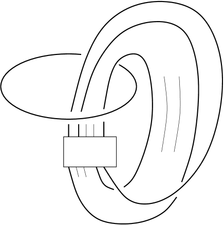
$-1$$k$$-1$$-k^{2}$

Figure 10. Surgery diagram for $S^{1}\times S^{2}$.

The contact manifold $(S^{1}\times S^{2},\xi_{k})$ is the boundary of the almost complex manifold $(X,J)$ obtained by attaching two $2$-handles to $D^{4}$ and forming the connected sum with ${\mathbb{C}}P^{2}$ (since we perform one contact $(+1)$-surgery), in particular, $c_{1}(\xi_{k})$ is the restriction of $c:=c_{1}(X,J)$ to the boundary.

Since $\mbox{\rm rot}(K_{1})=1$ and $\mbox{\rm rot}(K_{2})=k-2$, we have (with $[{\mathbb{C}}P^{1}]$ denoting the class of a complex line in the ${\mathbb{C}}P^{2}$ summand)

$$PD(c)=[N_{1}]+(k-2)[N_{2}]+3[{\mathbb{C}}P^{1}].$$

This implies

$$c_{1}(\xi_{k})=PD^{-1}([\mu_{1}]+(k-2)[\mu_{2}]).$$

With respect to the surface framing in $S^{3}$, the surgery coefficients are $n_{1}=\mbox{\rm tb}(K_{1})+1=-1$ and $n_{2}=\mbox{\rm tb}(K_{2})-1=-k^{2}$. Moreover, we have ${\ell k}(K_{1},K_{2})=k$. Thus the relations between $[\mu_{1}]$ and $[\mu_{2}]$ are given by

$$-[\mu_{1}]+k[\mu_{2}]=0,\;\;k[\mu_{1}]-k^{2}[\mu_{2}]=0.$$

Hence $[\mu_{2}]$ generates $H_{1}(S^{1}\times S^{2})$ and $c_{1}(\xi_{k})=(2k-2)PD^{-1}([\mu_{2}])$. ∎

A surgery diagram for an overtwisted contact structure $\xi_{0}$ on $S^{1}\times S^{2}$ with $c_{1}(\xi_{0})=0$ is given by the disjoint union of the knots in Figures 1 and 7. (This amounts to a connected sum of the tight contact structure on $S^{1}\times S^{2}$ with an overtwisted contact structure on $S^{3}$.)

By rotating the link diagram of Figure 9 by $180^{\circ}$ in the plane and keeping the orientations of $K_{1}$ and $K_{2}$, the rotation numbers change sign, while the homology classes $[\mu_{1}]$ and $[\mu_{2}]$ remain unchanged. So this provides surgery diagrams of contact structures $\xi_{-k}$ on $S^{1}\times S^{2}$ with first Chern class $c_{1}(\xi_{-k})=(2-2k)PD^{-1}[\mu_{2}]$, $k\geq 2$.

Notice that by reversing the orientations on the knots $K_{1}$ and $K_{2}$ of Figure 9 we could achive a sign change in the rotation numbers, implying a sign change in the coefficient of the expression for $c_{1}(\xi_{k})$. However, this change would also change the sign of $[\mu_{2}]$, so we would not have gained anything.

Here, again, is an alternative proof for the construction of all contact structures on $S^{1}\times S^{2}$; we leave it to the reader to check the details. Let $K_{0}$ be the Legendrian unknot of Figure 7 with $\mbox{\rm tb}(K_{0})=-1$. Let $K_{1}$ be a copy of this knot linked $k$ times with $K_{0}$. Let $K_{2}$ be a Legendrian push-off of $K_{1}$ with two zigzags added such that (with the appropriate choice of orientations) $\mbox{\rm rot}(K_{2})=\mbox{\rm rot}(K_{1})+2=2$. Contact $(+1)$-surgeries on $K_{0},K_{1},K_{2}$ give an overtwisted contact structure on $S^{1}\times S^{2}$ with $c_{1}=2kPD^{-1}[\mu_{0}]$, where the class of the normal circle $\mu_{0}$ to $K_{0}$ generates $H_{1}(S^{1}\times S^{2})$. That this surgery picture does indeed, topologically, describe $S^{1}\times S^{2}$ can be seen by sliding $K_{2}$ over $K_{1}$.

Overtwisted contact structures on $3$-manifolds

We now give an algorithm for drawing surgery diagrams for all overtwisted contact structures on an arbitrary given $3$-manifold $Y$. Recall from the discussion at the beginning of this section that we only need to find diagrams realising all spin^c structures.

Thus, assume that the 3-manifold $Y$ is given by surgery along a framed link

$$\mathbb{L}=((K_{1},n_{1}),\ldots,(K_{t},n_{t}))\subset S^{3}.$$

We may assume that these are honest surgeries, i.e. with integer framings $n_{i}$. If $Y$ is represented by Dehn surgeries (with rational coefficients) along a certain link, one can use continued fraction expansions of the surgery coefficients to turn the diagram into an integral surgery diagram as above. We retain the notation of Section 2, except that we allow ourselves to identify the normal circles $\mu_{i}$ with the homology classes they represent.

In order to find a contact surgery diagram for some contact structure on $Y$ we put the knots $K_{i}$ into Legendrian position relative to the standard contact structure on $S^{3}$. Write $b_{i}$ for the Thurston-Bennequin invariant $\mbox{\rm tb}(K_{i})$. If $n_{i}<b_{i}$, then by adding zigzags to the Legendrian knot $K_{i}$ (which decreases $b_{i}$) we can arrange $n_{i}=b_{i}-1$, hence contact $(-1)$-surgery on $K_{i}$ gives the desired result. If $n_{i}\geq b_{i}$ then we transform the Legendrian link near $K_{i}$ as shown in Figure 11, where $l_{i}=n_{i}-b_{i}$ and the surgery coefficients have to be read relative to the contact framing.

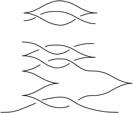
$\vdots$$K_{i,l_{i}}$$-1$$K_{i,l_{i}-1}$$-1$$K_{i,1}$$-1$$K_{i,0}$$+1$$K_{i}$$-1$

Figure 11. The first change on the surgery diagram.

Here is the verification that this does indeed correspond to a surgery along $K_{i}$ with framing $n_{i}$ (relative to the surface framing in $S^{3}$): First of all, we observe that the surgery coefficients relative to the surface framing are $-2$ for $K_{i,s}$, $s=1,\ldots,l_{i}$, for $K_{i,0}$ it is $-1$, and for $K_{i}$ it is $b_{i}-1$. We now slide off $K_{i,0},K_{i,1},\ldots,K_{i,l_{i}}$ (in this order). On sliding off $K_{i,0}$, the topological framing of $K_{i,1}$ (that is, the framing of the surgery relative to the surface framing of $K_{i,1}$) changes to $-2+1=-1$, that of $K_{i}$ to $b_{i}-1+1=b_{i}$, and $K_{i}$ becomes linked once with $K_{i,1}$. Continuing this way, each step produces a $(-1)$-framed unknot linked once with $K_{i}$. Finally, we end up with $l_{i}+1$ unknots with topological framing $-1$, which can be blown down, and with $K_{i}$ having framing $b_{i}-1+l_{i}+1=n_{i}$, as desired.

We claim that after the changes described in Figure 11 have been effected, the normal circles to $K_{i}$, $i=1,\ldots,t$, still generate $H_{1}(\partial X;{\mathbb{Z}})$: Choose orientations on $K_{i},K_{i,0},\ldots,K_{i,l_{i}}$ such that the intersection number of successive knots in this sequence equals $+1$ (this is only necessary to fix signs in the following computation). Write $\nu_{0},\ldots,\nu_{l}$ (we suppress the index $i$) for the homology classes represented by the normal circles to the knots $K_{i,0},\ldots,K_{i,l_{i}}$. These classes generate $H_{1}(\partial X;{\mathbb{Z}})$, and by Section 2 we have the following relations:

$$-2\nu_{l}+\nu_{l-1} = 0,$$

$$-2\nu_{i}+\nu_{i+1}+\nu_{i-1} = 0,\;\;i=1,\ldots,l-1,$$

$$-\nu_{0}+\nu_{1}+\mu_{i} = 0.$$

The second relation implies $\nu_{i+1}\in\langle\nu_{i},\nu_{i-1}\rangle$ for $i=1,\ldots,l-1$; the third relation yields $\nu_{1}\in\langle\nu_{0},\mu_{i}\rangle$. Finally, the relation provided by the Seifert surface of $K_{i}$ allows to express $\nu_{0}$ as a linear combination of $\mu_{1},\ldots,\mu_{t}$. In total, we see that all $\nu_{i,j}$ are contained in the linear span of the $\mu_{i}$ in $H_{1}(\partial X;{\mathbb{Z}})$.

We have thus found a contact $(\pm 1)$-surgery description for some contact structure on the given manifold $Y$. We now should like to perform further changes on that surgery diagram so as to realise all possible spin^c structures. The idea behind the following construction is first to introduce additional surgery curves such that (a) appropriate surgeries along these curves do not change the topology of $Y$ and (b) a subset of the additional surgery curves corresponds to a description of $S^{1}\times S^{2}$. Then the ideas used previously for $S^{1}\times S^{2}$ can be applied again.

Consider the contact manifold obtained by adding, for each $i=1,\ldots,t$, three surgery curves $K_{i,0}^{\prime},K_{i,1}^{\prime},K_{i,2}^{\prime}$ as indicated in Figure 12.

$K_{i,1}^{\prime}$$K_{i,0}^{\prime}$$K_{i,2}^{\prime}$$K_{i}$$-1$$-1$$+1$$+1$

Figure 12. The reference contact structure on $Y$.

Observe that the topological framings of $K_{i,0}^{\prime},K_{i,1}^{\prime},K_{i,2}^{\prime}$ are $0$, $-1$, and $-2$, respectively. Hence, with appropriate orientations on these knots and with $\mu_{0}^{\prime},\mu_{1}^{\prime},\mu_{2}^{\prime}$ denoting the homology classes represented by the normal circles to these knots (again we suppress the index $i$), we have the relations

$$0\cdot\mu_{0}^{\prime}+\mu_{2}^{\prime} = 0,$$

$$-\mu_{1}^{\prime} = 0,$$

$$-2\mu_{2}^{\prime}+\mu_{0}^{\prime}-\mu = 0,$$

that is, $\mu_{i,0}^{\prime}=\mu_{i}$ and $\mu_{i,1}^{\prime}=0=\mu_{i,2}^{\prime}$, $i=1,\ldots,t$. Observe that the surgery curve $K_{i,0}^{\prime}$ on its own gives a description of $S^{1}\times S^{2}$, with first homology group generated by $\mu_{i,0}^{\prime}$.

Topologically, these additional surgery curves do not change anything, so that we still have a description of $Y$: The $(-1)$-framed unknot $K_{i,1}^{\prime}$ gives a trivial surgery; a slam-dunk of $K_{i,0}^{\prime}$ changes the framing of $K_{i,2}^{\prime}$ to $\infty$, which again gives a trivial surgery. The presence of $K_{i,1}^{\prime}$ ensures that the diagram describes an overtwisted contact structure $\xi_{0}$ on $Y$, which will be our reference contact structure, inducing the spin^c structure $\mathbf{t}_{0}=\mathbf{t}_{\xi_{0}}$.

By viewing the knots in this diagram as attaching circles of $2$-handles rather than surgery curves, we can read the diagram as a description of a $4$-manifold $X$ with boundary $Y$. We have seen that, away from finitely many points, $X$ admits an almost complex structure $J$ such that $\xi_{0}=T\partial X\cap J(T\partial X)$. The corresponding spin^c structure $\mathbf{s}_{0}$ on $X$ restricts to $\mathbf{t}_{0}$ along $Y=\partial X$.

Given $\mathbf{t}\in Spin^{c}(Y)$ there is, thanks to the free and transitive action of $H^{2}(Y;{\mathbb{Z}})$ on $Spin^{c}(Y)$, a class $a_{\mathbf{t}}\in H^{2}(Y;{\mathbb{Z}})$ such that $\mathbf{t}=\mathbf{t}_{0}\otimes a_{\mathbf{t}}$. Since the restriction homomorphism $H^{2}(X;{\mathbb{Z}})\rightarrow H^{2}(Y;{\mathbb{Z}})$ is surjective (under Poincaré duality this corresponds to the surjectivity of $\varphi_{2}$ in Section 2), we may assume that $a_{\mathbf{t}}$ lives in $H^{2}(X;{\mathbb{Z}})$. Then $\mathbf{s}_{0}\otimes a_{\mathbf{t}}$ is a spin^c structure on $X$ that on $Y$ restricts to $\mathbf{t}$. The advantage of working over $X$ is that due to $\pi_{1}(X)=0$ the first Chern class captures the spin^c structure, whereas on $Y$ the identification of spin^c structures is complicated by the possible presence of $2$-torsion.

In conclusion, we need to find a contact surgery diagram that topologically yields $Y$ and such that the induced spin^c structure $\mathbf{s}$ on $X$ satisfies $c_{1}(\mathbf{s})=c_{1}(\mathbf{s}_{0})+2a_{\mathbf{t}}\in H^{2}(X;{\mathbb{Z}})$. Observe that because of $\mu_{i,0}^{\prime}=\mu_{i}$, we can — with $N_{i,0}^{\prime}$ denoting the normal disc bounded by $\mu_{i,0}^{\prime}$ — write $a_{\mathbf{t}}$ as

$$a_{\mathbf{t}}=\sum_{i=1}^{t}\alpha_{i}PD^{-1}[N_{i,0}^{\prime}]\in H^{2}(X;{\mathbb{Z}}).$$

If $\alpha_{i}=0$, we retain the diagram of Figure 12 near $K_{i}$. If $\alpha_{i}>0$, we use instead the diagram depicted in Figure 13, which is modelled on the one we used for $S^{1}\times S^{2}$.

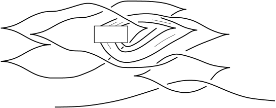
$+1$$-1$$-1$$K_{i,0}^{\prime\prime}$$-1$$K_{i}$$-1$$k_{i}-1$

Figure 13. The surgery diagram for $k_{i}=\alpha_{i}+1\geq 2$.

Observe that the presence of the (contact) $(+1)$-framed unknot with Thurston-Bennequin invariant $-2$ (and the fact that the other link components may be assumed not to intersect the overtwisted disc we exhibited in Figure 2) again ensures that the resulting contact structure is overtwisted. Moreover, the diagram is topologically equivalent to the one of Figure 12, with $K_{i,0}^{\prime\prime}$ taking the role of $K_{i,0}^{\prime}$. Thus, a calculation completely analogous to the one above for the contact structure $\xi_{k}$ on $S^{1}\times S^{2}$ shows that passing from the diagram in Figure 12 to the one in Figure 13 adds a summand $(2k_{i}-2)PD^{-1}[N_{i,0}^{\prime}]=2\alpha_{i}PD^{-1}[N_{i,0}^{\prime}]$ to the first Chern class of the corresponding spin^c structure.

For $\alpha_{i}<0$ one argues similarly, using the diagrams for the $\xi_{-k}$ instead. This concludes the construction of surgery diagrams for all overtwisted contact structures on the given $Y$.

Notice that when we claim to have found surgery diagrams for all overtwisted contact structures on a given (closed) $3$-manifold $Y$, we do of course rely on Eliashberg’s result [3] that overtwisted contact structures which are homotopic as $2$-plane fields are in fact isotopic as contact structures. However, our argument clearly provides an independent proof of the Lutz-Martinet theorem:

Corollary 4.6 (Lutz-Martinet).

On any given closed, orientable $3$-manifold, each homotopy class of $2$-plane fields contains an (overtwisted) contact structure. $\Box$

For an exposition of the original proof of that theorem, based on surgery along curves transverse to a given contact structure, see [11].

5. $(+1)$-surgery revisited

In this final section we briefly return to the issues raised in Remarks 3.3 and 3.5 concerning the extension of the almost complex structure over the handle and the value of $c(\Sigma)$ in the case of contact $(+1)$-surgery. In fact, most of our discussion in the present section relates to the translation from Weinstein’s description of contact surgery via symplectic handlebodies with contact type boundary to Eliashberg’s description via Stein manifolds (or complex handlebodies with strictly pseudoconvex boundary), and thus it applies equally well to the case of contact $(-1)$-surgery. Specifically, we address the question how to deform a handle in Weinstein’s picture so that the contact structure on the boundary of the handle is given by almost complex tangencies; we are not concerned with the more subtle point of the integrability of that almost complex structure (extending a given complex structure on the initial handlebody). The second issue then is to give a geometric description for the obstruction to extending that almost complex structure over the full handle in the case of contact $(+1)$-surgery – in the case of $(-1)$-surgery there is no such obstruction, as already discussed. We hope that the following considerations will prove useful in other instances where it may be opportune to switch between Eliashberg’s and Weinstein’s description of contact surgery.

We begin with the following simple lemma:

Lemma 5.1.

Let $E\rightarrow X$ be an oriented ${\mathbb{R}}^{4}$-bundle (over some manifold $X$) with bundle metric $g$ and $\xi\subset E$ an oriented ${\mathbb{R}}^{2}$-subbundle. Then there is a unique complex bundle structure $J$ on $E$ such that

• $g$ is $J$-invariant.

• $\xi$ is $J$-invariant

• $J$ induces the given orientations of $E$ and $\xi$.

Any two complex bundle structures $J_{0},J_{1}$ on $E$ satisfying (ii) and (iii) are homotopic.

Proof.

Let $(\sigma_{1},\sigma_{2},\sigma_{3},\sigma_{4})$ be an ordered quadruple of local $g$-orthonormal sections of $E$ with $(\sigma_{1},\sigma_{2})$ sections of $\xi$, inducing the given orientations. Then $J$ with the described properties can be defined by $J\sigma_{1}=\sigma_{2}$ and $J\sigma_{3}=\sigma_{4}$, and it is a straightforward check that this is the only way to define $J$.

Given $J_{0},J_{1}$ as described, let $g_{i}$, $i=0,1$, be a $J_{i}$-invariant bundle metric on $E$. The first part of the proof tells us that $J_{i}$ can be recovered from $g_{i}$. The complex bundle structure $J_{t}$ corresponding in this way to the bundle metric $g_{t}=(1-t)g_{0}+tg_{1}$, $t\in[0,1]$, defines a homotopy between $J_{0}$ and $J_{1}$. ∎

Recall from [2, Section 3] the description of contact $(+1)$-surgery as a symplectic handlebody surgery on the concave end of a symplectic cobordism: Consider ${\mathbb{R}}^{4}$ with cartesian coordinates $(x_{1},y_{1},x_{2},y_{2})$ and standard symplectic form

$$\omega=dx_{1}\wedge dy_{1}+dx_{2}\wedge dy_{2}.$$

Then

$$Z=2x_{1}\partial_{x_{1}}-y_{1}\partial_{y_{1}}+2x_{2}\partial_{x_{2}}-y_{2}\partial_{y_{2}}$$

is a Liouville vector field for $\omega$, that is, ${\mathcal{L}}_{Z}\omega=\omega$. This implies that $\alpha=i_{Z}\omega$ is a contact form on any hypersurface transverse to $Z$. Let $f\colon{\mathbb{R}}^{4}\rightarrow{\mathbb{R}}$ be the function defined by

$$f(x_{1},y_{1},x_{2},y_{2})=x_{1}^{2}-\frac{1}{2}y_{1}^{2}+x_{2}^{2}-\frac{1}{2}y_{2}^{2}$$

and set $Y_{\mu}=\{f=\mu\}$ and $S_{1}=Y_{1}\cap\{y_{1}=y_{2}=0\}$, which is Legendrian in $(Y_{1},\ker\alpha)$. A neighbourhood of $S_{1}$ in $Y_{1}$ can be identified with a neighbourhood of a given Legendrian knot $K$ in $(S^{3},\xi_{st})$ (which we take to be the boundary of $D^{4}$ with its standard complex structure $J$), and Figure 14 shows how to attach a symplectic handle $H$ along $S_{1}\equiv K$. (More generally, one can assume that $K$ is a Legendrian knot in a contact manifold $(Y,\xi)$ given as the boundary of an almost complex manifold $(X,J)$.) In [2] the framing of this surgery is computed to be indeed $+1$ with respect to the contact framing of $K$.

$S_{1}$$Z$$x_{1},x_{2}$$y_{1},y_{2}$$Y_{1}$$H$$U_{0}$$V_{0}$

Figure 14. Contact $(+1)$-surgery

The orientation of $Y_{1}$ is given by $\alpha\wedge d\alpha=i_{Z}\omega^{2}/2$. Hence, in order for $Y_{1}$ to carry the boundary orientation of $X_{1}=\{f\geq 1\}$, we need to equip ${\mathbb{R}}^{4}$ with the orientation given by $-\omega^{2}$ (or $-df\wedge\alpha\wedge d\alpha$).

A complex bundle structure $J_{0}$ on $E=T({\mathbb{R}}^{4}-\{0\})$ is defined, in the sense of the preceding lemma, by the $2$-plane bundle

$$\xi_{0}=\ker df\cap\ker\alpha$$

(oriented by $d\alpha$) and the standard metric $g_{0}$ on ${\mathbb{R}}^{4}$. Then on each level surface $Y_{\mu}$ (except at the singular point $0\in Y_{0}$), the contact structure $\xi_{0}$ coincides with the $J_{0}$-complex tangencies of $Y_{\mu}$.

Proposition 5.2.

In the notation of Proposition 3.4, we have $c(\Sigma)=\mbox{\rm rot}(K)$, independently of the value of $\mbox{\rm tb}(K)$.

Proof.

We should like to argue that $J_{0}$ does in fact define the extension $J$ of the almost complex structure on $D^{4}$ over $H-\{0\}$. Unfortunately, this is not quite true, since the boundary of $H$ is not a level surface of $f$, so the contact structure $\ker\alpha\cap T(\partial H)$ on $\partial H$ does not coincide with $\xi_{0}$, i.e. that contact structure is not given by the $J_{0}$-complex tangencies of $\partial H$. Up to homotopy, however, this is essentially true. Thus, before addressing this mild subtlety, we prove that $c(\Sigma)=\mbox{\rm rot}(K)$ from the $J=J_{0}$ as described.

Let $F$ be the Seifert surface of $K$ in $S^{3}$ and $D$ the core disc of $H$,

$$D=\{(x_{1},y_{1},x_{2},y_{2})\colon x_{1}^{2}+x_{2}^{2}\leq 1,\;y_{1}=y_{2}=0\},$$

perturbed slightly around $0$ so that it stays inside $H$ but misses the origin of ${\mathbb{R}}^{4}$. Then $\Sigma$, by definition, is the surface obtained by gluing $F$ and $D$ along $S_{1}\equiv K$, with orientation of $K$ equal to the boundary orientation of $F$.

Along $S^{3}$ the tangent bundle of $D^{4}$ splits (as a complex bundle) into the complex line bundle $\xi_{st}$ and a trivial complex line bundle defined by the complex lines containing the outward normal. That latter trivialisation extends to a trivialisation of a complex line bundle in $T{\mathbb{R}}^{4}|_{D}$ complementary to $\xi_{0}|_{D}$, viz., the $J_{0}$-complex lines containg $Z$. Therefore the first Chern class $c$ of $J$, when restricted to $\Sigma$, equals the first Chern class of $\xi|_{\Sigma}$ (with $\xi=\xi_{st}$ on $F$ and $\xi=\xi_{0}$ on $D$).

Moreover, the vector field

$$v=2x_{2}\partial_{x_{1}}+y_{2}\partial_{y_{1}}-2x_{1}\partial_{x_{2}}-y_{1}\partial_{y_{2}}$$

is a nowhere zero vector field in $\xi_{0}|_{H-\{0\}}$ – in particular, it defines a trivialisation of the complex line bundle $\xi_{0}|_{D}$ – and its restriction to $S_{1}$ is tangent to that circle. By our orientation assumption on $K\equiv S_{1}$ and $F$, the value $c(\Sigma)=\langle c_{1}(\xi|_{\Sigma}),[\Sigma]\rangle$ is equal to the rotation number of $v|_{K}$ relative to a trivialisation of $\xi_{st}|_{F}$, which by definition is precisely $\mbox{\rm rot}(K)$. ∎

We now show how to deform the local picture of Figure 14 in such a way that the extension of the almost complex structure over $H-\{0\}$ is indeed defined by $J_{0}$.

First of all, we have a contactomorphism $\varphi$ from a neighbourhood of $K$ in $(S^{3},\xi_{st})$ to a neighbourhood of $S_{1}$ in $(Y_{1},\xi_{0})$. Extend $\varphi$ to a diffeomorphism of a neighbourhood of $K$ in $D^{4}$ to a neighbourhood of $S_{1}$ in $X_{1}$. We claim that one can homotope $J$ on $D^{4}$ to an almost complex structure (still denoted $J$) such that

• $\xi_{st}$ is still given by the $J$-complex tangencies of $S^{3}=\partial D^{4}$,

• the homotopy is supported in a given neighbourhood of $K$ in $D^{4}$,

• $\varphi_{*}J$ coincides with $J_{0}$ in a neighbourhood $U_{0}$ of $S_{1}$ in $X_{1}$.

In order to see this, extend $\xi_{st}$ to a plane field $\xi$ on $D^{4}-\{0\}\subset{\mathbb{C}}^{2}$ as the complex tangencies of the spheres of radius $r\in(0,1]$. Since $\xi_{st}$ coincides with $\varphi^{*}\xi_{0}$ on a neighbourhood of $K$ in $S^{3}$, there is a homotopy of $\xi$, fixed on $S^{3}$ and supported in a neighbourhood of $K$ in $D^{4}$, to a plane field (still denoted $\xi$) that coincides with $\varphi^{*}\xi_{0}$ in a (smaller) neighbourhood $U$ of $K$ in $D^{4}$. Clearly, there is a corresponding homotopy of the standard metric on $D^{4}$ to a metric coinciding with $\varphi^{*}g_{0}$ near $K$. Lemma 5.1 then allows us to construct the desired homotopy of $J$, with $U_{0}=\varphi(U)$.

We attach the handle $H$ inside the neighbourhood $U_{0}\cap Y_{1}$. Next choose a smaller neighbourhood $V_{0}\subset U_{0}$ of $S_{1}$ in $X_{1}$ such that $V_{0}\cap Y_{1}$ lies completely inside the region where $H$ is attached to $X_{1}$. Let $h_{0}\colon{\mathbb{R}}^{4}-\{0\}\rightarrow{\mathbb{R}}^{-}$ be the function

$$h_{0}(x_{1},y_{1},x_{2},y_{2})=-\frac{2}{4x_{1}^{2}+y_{1}^{2}+4x_{2}^{2}+y_{2}^{2}},$$

and $h\colon{\mathbb{R}}^{4}\rightarrow{\mathbb{R}}^{-}$ a smooth function such that $h=h_{0}$ outside a neighbourhood of the origin chosen so small that the flow $\varphi_{t}$ of $hZ$ coincides with the flow of $h_{0}Z$ on a collar neighbourhood $W_{0}$ of $Y_{1}-\overline{V_{0}}$ in $X_{1}$. Notice that since the flow $\varphi_{t}$ of $hZ$ is simply a reparametrisation of the flow of $Z$, hypersurfaces transverse to $Z$ stay transverse to $Z$ and continue to inherit a contact structure from the $1$-form $\alpha=i_{Z}\omega$.

Observe that ${\mathcal{L}}_{hZ}\alpha=i_{hZ}d\alpha=h\alpha$, so the flow $\varphi_{t}$ of $hZ$ preserves $\ker\alpha$. Furthermore, $df(h_{0}Z)\equiv-2$. This implies that $\varphi_{t}(Y_{1}-\overline{V_{0}})\subset Y_{1-2t}$ and

$$\varphi_{t*}(\ker df_{x}\cap\ker\alpha_{x})=\ker df_{\varphi_{t}(x)}\cap\ker\alpha_{\varphi_{t}(x)}\;\;\mbox{\rm for}\;x\in W_{0},$$

in particular, the map $\varphi_{t}\colon Y_{1}-\overline{V_{0}}\rightarrow Y_{1-2t}$ is an embedding preserving the contact structure $\xi_{0}$ on the respective hypersurfaces.

So $\varphi^{*}\varphi_{t}^{*}\xi_{0}$ (on $\varphi^{-1}(U_{0})=U$) is a homotopy of $\varphi^{*}\xi_{0}=\xi$ that stays constant in the collar neighbourhood $\varphi^{-1}(W_{0})$ of $S^{3}\cap\varphi^{-1}(U_{0}-\overline{V_{0}})$. This allows to spread out that homotopy over a collar of $S^{3}$ in $D^{4}$ so as to obtain a plane field (still denoted $\xi$) on $D^{4}-\{0\}$ that is homotopic to the old $\xi$ under a homotopy supported in a neighbourhood of $K$ in $D^{4}$. Once again, Lemma 5.1 defines a corresponding homotopy of $J$ (since one can always interpolate between different metrics).

Thus, after such a homotopy of $J$ and a homotopy of $\xi_{st}$ defined by $\ker\varphi^{*}\varphi_{t}^{*}\alpha|_{TS^{3}}$, fixed outside $S^{3}\cap\varphi^{-1}(\overline{V_{0}})$, we may assume that $\varphi_{1}\circ\varphi$ sends $S^{3}\cap\varphi^{-1}(U_{0})$ contactomorphically into $\varphi_{1}(Y_{1})$ and that $\varphi_{1}\circ\varphi$ is a $J$-$J_{0}$-holomorphic map on a collar neighbourhood of $S^{3}\cap\varphi^{-1}(U_{0})$ in $D^{4}$. Notice, however, that $\ker\varphi^{*}\varphi_{1}^{*}\alpha|_{TS^{3}}$ need no longer coincide on $\varphi^{-1}(\overline{V_{0}})$ with the (homotoped) $J$-complex tangencies, and $(\varphi_{1}\circ\varphi)_{*}\xi_{st}$ may not coincide with the $J_{0}$-complex tangencies of $\varphi_{1}(Y_{1}\cap\overline{V_{0}})$.

Now define $H^{\prime}$ to be the region bounded by $Y_{-1}$ and $\varphi_{1}(Y_{1})$; this really amounts to a deformation of $\varphi_{1}(H)$ keeping its boundary transverse to $Z$, hence to a contact isotopy of the surgered contact manifold. This $H^{\prime}$ defines contact $(+1)$-surgery in such a way that the extension of the almost complex structure over $H^{\prime}-\{0\}$ is defined by $J_{0}$.

Finally, we want to give a more geometric argument for the extendability of the almost complex structure $J_{0}$ on $H-\{0\}$ to $H\#{\mathbb{C}}P^{2}$; this gives a new proof of the statement $d_{3}(\xi_{H})=1/2$ in Proposition 3.4, independently of the value of $\mbox{\rm tb}(K)$.

To that end, consider the map $\pi\colon{\mathbb{R}}^{4}\rightarrow{\mathbb{C}}$ given by $\pi(x_{1},y_{1},x_{2},y_{2})=z_{1}^{2}+z_{2}^{2}$, where we set $z_{1}=x_{1}+iy_{1}$ and $z_{2}=x_{2}+iy_{2}$. Write $\pi_{1},\pi_{2}$ for the real and imaginary part of $\pi$, respectively, i.e.

$$\pi_{1}(x_{1},y_{1},x_{2},y_{2}) = x_{1}^{2}-y_{1}^{2}+x_{2}^{2}-y_{2}^{2},$$

$$\pi_{2}(x_{1},y_{1},x_{2},y_{2}) = 2x_{1}y_{1}+2x_{2}y_{2}.$$

Then

$$d\pi_{1} = 2x_{1}dx_{1}-2y_{1}dy_{1}+2x_{2}dx_{2}-2y_{2}dy_{2},$$

$$d\pi_{2} = 2x_{1}dy_{1}+2y_{1}dx_{1}+2x_{2}dy_{2}+2y_{2}dx_{2}.$$

There is an obvious linear homotopy on ${\mathbb{R}}^{4}-\{0\}$ between the pair $(df,\alpha)$ and the pair $(d\pi_{1},d\pi_{2})$, the homotopy being through linearly independent pairs of $1$-forms. Therefore, $J_{0}$ is homotopic, by Lemma 5.1, to the almost complex structure $J_{1}$ determined by the plane field $\ker d\pi_{1}\cap\ker d\pi_{2}$, coorientation given by $-d\pi_{1}\wedge d\pi_{2}$, and ambient orientation given by $-\omega^{2}$. This $J_{1}$ is exactly the almost complex structure near an incorrectly oriented critical point (excluding that point) of an achiral Lefschetz fibration, see [13, Section 8], and Lemma 8.4.12 of the cited reference provides a geometric argument, based on work of Matsumoto, for the extendability of $J_{1}$ over the connected sum with a copy of ${\mathbb{C}}P^{2}$.

Acknowledgements. F. D. is partially supported by grant no. 10201003 of the National Natural Science Foundation of China. H. G. is partially supported by grant no. GE 1254/1-1 of the Deutsche Forschungsgemeinschaft within the framework of the Schwerpunktprogramm 1154 “Globale Differentialgeometrie”. A. S. is partially supported by OTKA T034885.

H. G. and A. S. acknowledge the support of TUBITAK for attending the 10th Gökova Geometry-Topology conference, which allowed us to discuss some of the final details of this paper.

References

- [1] F. Ding and H. Geiges, Symplectic fillability of tight contact structures on torus bundles, Alg. and Geom. Topol. 1 (2001), 153–172.
- [2] F. Ding and H. Geiges, A Legendrian surgery presentation of contact -manifolds, Math. Proc. Cambridge Philos. Soc., to appear.
- [3] Ya. Eliashberg, Classification of overtwisted contact structures on -manifolds, Invent. Math. 98 (1989), 623–637.
- [4] Ya. Eliashberg, Topological characterization of Stein manifolds of dimension , International J. of Math. 1 (1990), 29–46.
- [5] Ya. Eliashberg, Contact -manifolds twenty years since J. Martinet’s work, Ann. Inst. Fourier (Grenoble) 42 (1992), 165–192.
- [6] Ya. Eliashberg, Legendrian and transversal knots in tight contact -manifolds, in: Topological Methods in Modern Mathematics (Stony Brook, 1991), Publish or Perish, Houston (1993), 171–193.
- [7] J. Etnyre, Introductory lectures on contact geometry, in: Proc. Georgia Topology Conference (Athens, GA, 2001), to appear.
- [8] J. Etnyre, Legendrian and transversal knots, in: Handbook of Knot Theory, Elsevier, to appear.
- [9] J. Etnyre and K. Honda, On symplectic cobordisms, Math. Ann. 323 (2001), 31–39.
- [10] F. Forstnerič and J. Kozak, Strongly pseudoconvex handlebodies, arXiv: math. CV/0305237.
- [11] H. Geiges, Contact geometry, in: Handbook of Differential Geometry vol. 2 (F.J.E. Dillen and L.C.A. Verstraelen, eds.), Elsevier, to appear.
- [12] R. E. Gompf, Handlebody construction of Stein surfaces, Ann. of Math. 148 (1998), 619–693.
- [13] R. E. Gompf and A. I. Stipsicz, -manifolds and Kirby calculus, Grad. Stud. in Math. 20, Amer. Math. Soc., Providence, 1999.
- [14] K. Honda, On the classification of tight contact structures I, Geom. Topol. 4 (2000), 309–368.
- [15] Y. Kanda, The classification of tight contact structures on the -torus, Comm. Anal. Geom. 5 (1997), 413–438.
- [16] G. Kuperberg, Noninvolutory Hopf algebras and -manifold invariants, Duke Math. J. 84 (1996), 83–129.
- [17] P. Lisca and A. I. Stipsicz, Tight, not semi-fillable contact circle bundles, arXiv: math.SG/0211429.
- [18] P. Lisca and A. I. Stipsicz, Heegaard Floer invariants and tight contact three-manifolds, arXiv: math.SG/0303280.
- [19] V. Turaev, Torsion invariants of -structures on -manifolds, Math. Res. Lett. 4 (1997), 679–695.
- [20] A. Weinstein, Contact surgery and symplectic handlebodies, Hokkaido Math. J. 20 (1991), 241–251.