Unimodal generalized pseudo-Anosov maps

Abstract

An infinite family of generalized pseudo-Anosov homeomorphisms of the sphere $S$ is constructed, and their invariant foliations and singular orbits are described explicitly by means of generalized train tracks. The complex strucure induced by the invariant foliations is described, and is shown to make $S$ into a complex sphere. The generalized pseudo-Anosovs thus become quasiconformal automorphisms of the Riemann sphere, providing a complexification of the unimodal family which differs from that of the Fatou/Julia theory.

andre@ime.usp.brandT.Hall@liv.ac.uk

37E30 57M50

$\cal G\mskip-2.0mu$eometry & $\cal T\!\!$opology $\cal G$$\cal G$$\cal G$$\cal G$$\cal G$$\cal G$$\cal G$$\cal G$$\cal G$$\cal G$$\cal G$$\cal G$$\cal G$$\cal G$$\cal G$$\cal T$$\cal T$$\cal T$$\cal T$$\cal T$$\cal T$$\cal T$$\cal T$$\cal T$$\cal T$$\cal T$$\cal T$$\cal T$$\cal T$$\cal T$Volume 8 (2004) 1127–1188Published: 8 September 2004

Email: URL:

Abstract

AMS Classification numbers Primary: 

Secondary: 

Keywords: 

Proposed: Joan Birman Received: 10 July 2003Seconded: David Gabai, Yasha Eliashberg Revised: 4 February 2004

1 Introduction

1.1 Overview

Pseudo-Anosov homeomorphisms were introduced by Thurston in his classification of surface homeomorphisms up to isotopy. A surface homeomorphism $\Phi\co S\includegraphics[height=7.22743pt]{backarr.eps}$ is pseudo-Anosov if it preserves a transverse pair of measured foliations with finitely many singularities, expanding one foliation uniformly by a factor $\lambda>1$ and contracting the other by a factor $1/\lambda$. Pseudo-Anosov maps can be described combinatorially by train tracks — a class of graphs embedded in the surface with additional information on the vertices which specifies the turns a train riding along the track can make at each vertex — and their endomorphisms. Using information obtained from an associated transition matrix, the surface can be reconstructed by identifying sides of Euclidean rectangles foliated by horizontal and vertical line segments. The pseudo-Anosov expands the rectangles horizontally and contracts them vertically, mapping them as dictated by the train track map. Up to this point, the discussion is finite: train tracks are graphs with finitely many edges (Thurston’s theorem can be proved algorithmically, the main step being to find a finite train track invariant under a given isotopy class of homeomorphisms) and train track maps are finite-to-one. It is possible, however, to forgo some of the finiteness requirements — the graphs remain finite, the endomorphisms remain finite-to-one, but the additional information at the vertices is allowed to be infinite — but otherwise to go through the construction of the maps as before. This leads to the construction of generalized pseudo-Anosov homeomorphisms. These are defined similarly to pseudo-Anosov homeomorphisms, except that the invariant foliations are permitted to have infinitely many singularities, provided that they accumulate on only finitely many points. The purpose of this paper is to give a detailed construction and description of an infinite family of generalized pseudo-Anosovs of the sphere for which the underlying graph and graph map are the simplest possible: an interval and a unimodal endomorphism (ie, a continuous piecewise monotone map of the interval with exactly two monotone pieces).

In [12], a complete description of the family of pseudo-Anosov maps with underlying unimodal interval endomorphisms was given. It was shown that there is a countable family of such maps parameterized by a rational number between 0 and 1/2, called height. Height turns out to be a braid type invariant and this leads to the proof of weak universality results for families of plane homeomorphisms passing from trivial to chaotic dynamics as parameters are varied. Height also plays a central role in this paper and, in turn, the results presented here provide a geometric interpretation of it. The family of unimodal generalized pseudo-Anosovs extends that of unimodal pseudo-Anosovs. The height specifies the behaviour of the maps at infinity: given a rational $m/n$, there is an interval of kneading sequences of height $m/n$, whose associated generalized pseudo-Anosovs have the same behaviour at infinity. The generalized pseudo-Anosov is a pseudo-Anosov for exactly one kneading sequence in this interval.

This paper provides an explicit description of the generalized train track associated to any periodic or preperiodic kneading sequence, depending crucially on its height. The process of constructing a generalized pseudo-Anosov from a generalized train track map is similar to that of constructing a pseudo-Anosov from a train track map, but requires more care because of the more intricate nature of the identifications carried out on the sphere. The topological tool used to guarantee that the identification space is again a sphere is Moore’s theorem about monotone upper semi-continuous decompositions of the sphere.

The invariant foliations of a generalized pseudo-Anosov define a complex structure on the sphere away from the accumulations of singularities. It is shown that for the unimodal generalized pseudo-Anosovs considered here, these accumulations are removable singularities of the complex structure, so that the sphere is a complex sphere, with the foliations being the horizontal and vertical trajectories of an integrable quadratic differential having infinitely many zeros and poles. The construction therefore provides a complexification of unimodal maps as quasiconformal automorphisms of the Riemann sphere, in contrast to the complexification arising via the theory of Fatou/Julia, where one thinks of the unimodal map as the real slice of an endomorphism of the Riemann sphere.

By a suitable normalization, the sphere of definition of the generalized pseudo-Anosovs can be identified canonically with the Riemann sphere, and hence the family of unimodal generalized pseudo-Anosovs, which initially are constructed on abstract topological spheres, can be regarded as a family of Teichmüller mappings of the Riemann sphere, making it possible to consider taking limits within the family. This is a necessary step in the problem of constructing a completion of the set of all pseudo-Anosov homeomorphisms of the sphere.

Section 2 describes the class of thick interval maps. These are homeomorphisms of the sphere which provide the starting point for the definition and construction of invariant generalized train tracks, a process which is described in Section 3. Section 4 provides a summary of necessary results on unimodal maps and Smale’s horseshoe, and defines the subclass of unimodal thick interval maps which are used in the remainder of the paper. In Section 5, the outside dynamics of a unimodal map is defined and analysed: intuitively, this provides a description of those orbits of a unimodal map which are never lost ‘inside’ the fold. The main contents of the paper can be found in Sections 6, 7 and 8. The invariant generalized train track for a given unimodal thick interval map is described explicitly, a detailed account is given of how the generalized train track map can be used to construct the corresponding generalized pseudo-Anosov, and the complex structure induced by the invariant foliations is analysed.

AcknowledgementsThe authors are grateful for the referee’s careful reading of the paper and helpful comments. This material is based upon work supported by the National Science Foundation under Grant No. 0203975. The first author is supported by FAPESP Grant No. 02/05072-5.

1.2 Definitions and notation

Let $X$ be a metric space. An isotopy on $X$ is a continuous map $\psi\co X\times[0,1]$$\to X$ with the property that the slice maps $\psi_{t}\co X\to X$ are homeomorphisms for $0\leq t\leq 1$. A pseudo-isotopy is defined similarly but it is only required that the slice maps be homeomorphisms for $0\leq t<1$. In particular, this means that the map $\psi_{1}$ is a near-homeomorphism, ie, it can be approximated arbitrarily closely by homeomorphisms. An isotopy or pseudo-isotopy $\psi\co X\times[0,1]\to X$ is said to be supported on a subset $U$ of $X$ if all of its slice maps agree on $X\setminus U$.

Symbolic dynamics on both $\{0,1\}^{\mathbb{N}}$ and $\{0,1\}^{\mathbb{Z}}$ will be used in this paper. Elements of these spaces are regarded as semi-infinite or bi-infinite sequences of $0$s and $1$s, and in the case of $\{0,1\}^{\mathbb{Z}}$ a period is placed before the origin of the sequence (ie, the image of $0\in\mathbb{Z}$): $\ldots s_{-2}s_{-1}\cdot s_{0}s_{1}s_{2}\ldots\in\{0,1\}^{\mathbb{Z}}$. If $w\in\{0,1\}^{n}$ for some $n$, then the notation $w^{\infty}$ is used to indicate semi-infinite repetition of $w$ ($w^{\infty}=wwww\ldots\in\{0,1\}^{\mathbb{N}}$), while $\overline{w}$ is used to indicate bi-infinite repetition ($\overline{w}=\ldots www\cdot www\ldots\in\{0,1\}^{\mathbb{Z}}$).

The notation $S^{1}$ and $S^{2}$ is reserved for the standard 1- and 2-dimensional spheres, and different symbols are used to denote general topological spheres.

A homeomorphism $\Phi\co S\includegraphics[height=7.22743pt]{backarr.eps}$ of a smooth surface $S$ is called a generalized pseudo-Anosov map if there exist

1. a finite $\Phi$-invariant set $\Sigma$;

2. a pair $({\mathcal{F}}^{s},\mu^{s})$, $({\mathcal{F}}^{u},\mu^{u})$ of transverse measured foliations of $S\setminus\Sigma$ with countably many pronged singularities (with local charts as depicted in Figure 1), which accumulate on each point of $\Sigma$ and have no other accumulation points. The transverse measures are required to be equivalent to Lebesgue measure on transversals;

3. a real number $\lambda>1$;

such that

$$\begin{array}[]{ccc}\Phi({\mathcal{F}}^{s},\mu^{s})&=&({\mathcal{F}}^{s},\frac{1}{\lambda}\mu^{s})\\ \Phi({\mathcal{F}}^{u},\mu^{u})&=&({\mathcal{F}}^{u},\lambda\mu^{u}).\end{array}$$

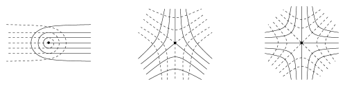
Figure 1: Pronged singularities of the invariant foliations

In particular, a generalized pseudo-Anosov is a pseudo-Anosov map if and only if there are only finitely many pronged singularities (ie, $\Sigma=\emptyset$). Note that the measures necessarily have full support and no atoms.

2 Markov thick interval maps

2.1 Thick interval maps

Thick graph maps are a class of surface homeomorphisms which have been described and used in several papers (for example [2, 5, 10, 4]). In this section a brief description of thick interval maps (where the surface is the sphere and the graph is an interval) is given. As the name suggests, a thick interval map is essentially an interval endomorphism which has been thickened up and made into a homeomorphism of the sphere, whose dynamics reflects that of the underlying interval map.

Throughout the paper, $S^{2}$ will be thought of as the one-point compactification of $\mathbb{R}^{2}$. The point at infinity will be denoted $\infty$ and the thick intervals defined below will always be assumed not to contain $\infty$.

Definitions 1.

A thick interval $\mathbb{I}\subset S^{2}$ is a closed topological $2$-disk partitioned into compact decomposition elements, such that

1. each decomposition element of $\mathbb{I}$ is either a leaf homeomorphic to $[0,1]$, or a junction homeomorphic to a closed $2$-disk;

2. the boundary in $\mathbb{I}$ of each junction consists of one or two disjoint arcs: if there is one (respectively two) such arc(s) the junction is called a 1-junction (respectively 2-junction);

3. there are exactly two 1-junctions and finitely many 2-junctions;

4. each decomposition element is contained in a chart as depicted in Figure 2.

If $\mathbb{I}$ is a thick interval, then the space obtained by collapsing each decomposition element to a point is an interval, whose vertices (the two endpoints, coming from the two 1-junctions, and finitely many valence $2$ vertices) correspond to the junctions of $\mathbb{I}$. The union of the junctions of $\mathbb{I}$ is denoted $\mathbb{V}$, and the components of $\mathbb{I}\setminus\mathbb{V}$ are called strips: each strip is therefore homeomorphic to $(0,1)\times[0,1]$. The union of the closures of the strips is denoted $\mathbb{E}$. Thus $\mathbb{E}\cap\mathbb{V}$ is a union of closed arcs which are the boundary components (in $\mathbb{I}$) of both the junctions and the strips of $\mathbb{I}$.

\psfrag{1}[t]{$1$-junction}\psfrag{2}[t]{$2$-junction}\psfrag{l}[b]{leaves}\includegraphics[width=260.17464pt]{charts}

Figure 2: Charts in a thick interval

The following definition of a thick interval map is more restrictive than that used in other papers: conditions iv) to vi) have been added in order to make the definition and construction of generalized train tracks more straightforward. However, thick interval maps in the sense of [5] can be made to conform to the definition below by simple isotopies and changes in the thick interval structure which do not change the dynamics. In order to make the description more explicit, fixed orientation-preserving coordinate maps $h_{s}\co\overline{s}\to[0,1]\times[0,1]$ are introduced on the closure of each strip $s$, with the property that the leaves of $s$ are of the form $h_{s}^{-1}(\{x\}\times[0,1])$ for $0<x<1$.

Definition 2.

A thick interval map is an orientation-preserving homeomorphism $F\co(S^{2},\mathbb{I})\includegraphics[height=7.22743pt]{backarr.eps}$ such that:

1. $F(\mathbb{I})\subset\operatorname{Int}(\mathbb{I})$.

2. If $\gamma$ is a leaf of $\mathbb{I}$, then $F(\gamma)$ is contained in a decomposition element, and $\operatorname{diam}(F^{n}(\gamma))\to 0$ as $n\to\infty$. If $J$ is a junction of $\mathbb{I}$, then $F(J)$ is contained in a junction.

3. The point at infinity is a repelling fixed point whose basin contains $S^{2}\setminus\mathbb{I}$.

4. $F$ is linear with respect to the coordinates $h_{s}$: in each connected component of $s_{i}\cap F^{-1}(s_{j})$, where $s_{i}$, $s_{j}$ are strips, $F$ contracts vertical coordinates uniformly by a factor $\mu_{j}<1$ and expands horizontal coordinates uniformly by a factor ${\lambda}_{j}\geq 1$;

5. If $J,J^{\prime}$ are junctions such that $F(J)\subset J^{\prime}$, then $F(\partial_{\mathbb{I}}J)\subset\partial_{\mathbb{I}}J^{\prime}$;

6. If $J$ is a junction with $F^{n}(J)\subseteq J$ for some (least) $n\geq 1$, then $J$ has an attracting periodic point of least period $n$ in its interior whose basin contains $\operatorname{Int}(J)$.

Remark 1.

Item iii) in the definition says that the dynamics of a thick interval map in $S^{2}\setminus\mathbb{I}$ is easily understood and uninteresting.

Let $F\co(S^{2},\mathbb{I})\includegraphics[height=7.22743pt]{backarr.eps}$ be a thick interval map, $\tilde{I}$ be the interval obtained by collapsing each decomposition element of $\mathbb{I}$ to a point, and $\tilde{\pi}\co\mathbb{I}\to\tilde{I}$ be the canonical projection. Then $F$ induces a continuous map $\tilde{f}\co\tilde{I}\includegraphics[height=7.22743pt]{backarr.eps}$: however $\tilde{f}$ is locally constant at preimages of $\tilde{\pi}(\mathbb{V})$. It is therefore convenient to collapse all intervals on which some iterate ${\tilde{f}}^{n}$ is constant. Because closed intervals are collapsed to points, the quotient of the interval $\tilde{I}$ is either a point or an interval $I$. In the latter case $\tilde{f}$ induces a continuous piecewise strictly monotone interval map $f\co I\includegraphics[height=7.22743pt]{backarr.eps}$, which is called the quotient of $F\co(S^{2},\mathbb{I})\includegraphics[height=7.22743pt]{backarr.eps}$. All thick interval maps considered in this paper will have an interval map for quotient (see Section 2.2). Note that if $\pi\co\mathbb{I}\to I$ denotes the canonical projection, then $\pi\circ F|_{\mathbb{I}}=f\circ\pi$.

Example 1.

The first example is Smale’s horseshoe map which will be denoted $F_{0}\co(S^{2},\mathbb{I})\includegraphics[height=7.22743pt]{backarr.eps}$ here and in what follows. It is shown in Figure 3. The horseshoe has three fixed points, denoted $x$, $x_{0}$, and $x_{1}$. The fixed point $x$ is attracting (condition vi)), while $x_{0}$ and $x_{1}$ are saddles by conditions iv) and vi). The quotient interval map — the tent map $f_{0}\co I\includegraphics[height=7.22743pt]{backarr.eps}$ — is also shown in the figure.

\psfrag{tp}{$\scriptstyle{\tilde{\pi}}$}\psfrag{tf}{$\scriptstyle{\tilde{f}_{0}}$}\psfrag{p}{$\scriptstyle{\pi}$}\psfrag{T}[l]{$\scriptstyle{\mathbb{I}}$}\psfrag{F}{$\scriptstyle{F_{0}}$}\psfrag{f}{$\scriptstyle{f_{0}}$}\psfrag{x}{$\scriptstyle{x}$}\psfrag{y}{$\scriptstyle{x_{0}}$}\psfrag{z}{$\scriptstyle{x_{1}}$}\includegraphics[width=173.44534pt]{gpA_hs}

Figure 3: The horseshoe map

Example 2.

Figure 4 depicts an example of a thick interval map associated to a horseshoe periodic orbit: such thick interval maps are the starting point for the construction of unimodal generalized train tracks described in Section 6. The interval endomorphism $f$ is one with kneading sequence $\kappa(f)=(1001011)^{\infty}$ (see Section 4).

\psfrag{F}[bl]{$\scriptstyle{F}$}\psfrag{f}[l]{$\scriptstyle{f}$}\includegraphics[width=346.89731pt]{thtrmap}

Figure 4: A thick interval map associated to a horseshoe periodic orbit

2.2 The MIA property

First the basic concepts of the Perron-Frobenius theory for non-negative integer matrices are described (see [11]). Let $M$ be a square matrix with non-negative integer entries, which is not equal to the $1\times 1$ matrix $(1)$. $M$ is said to be reducible if, by a permutation of the index set, it is possible to put it in triangular block form:

$$M=\left(\begin{array}[]{cc}A&0\\ B&C\end{array}\right),$$

with $A$ and $C$ non-trivial square matrices. Otherwise, $M$ is said to be irreducible. An irreducible matrix $M$ has a unique positive eigenvector (up to scaling), and the associated eigenvalue $\lambda$, called the Perron-Frobenius eigenvalue of $M$, is simple and is equal to the spectral radius of $M$. $M$ is irreducible and aperiodic if there is a positive integer $k$ such that every entry of $M^{k}$ is positive. In this case the Perron-Frobenius eigenvalue $\lambda$ satisfies $\lambda>1$, and is the only eigenvalue of $M$ on the circle $\{z\in\mathbb{C}\,:\,|z|=\lambda\}$.

Let $F\co(S^{2},\mathbb{I})\includegraphics[height=7.22743pt]{backarr.eps}$ be a thick interval map. Associate a transition matrix $M=\left(m_{ij}\right)$ to $F$ in the following way: let $s_{1},s_{2},\ldots,s_{n}$ be the strips of $\mathbb{I}$ and set

$$m_{ij}=\mbox{number of times\ }F(s_{j})\mbox{\ crosses\ }s_{i}.$$

Definition 3.

A thick interval map is MIA if its associated transition matrix is irreducible and aperiodic (the ‘M’ stands for Markov).

If $F$ is MIA then the quotient interval $I$ is not a point, and indeed the projection $\pi(s_{j})$ of each strip of $\mathbb{I}$ is a non-trivial interval. For there are integers $n_{j}$ such that $F^{n_{j}}(s_{j})$ crosses $s_{j}$ at least twice, with horizontal expansion and vertical contraction bounded away from $1$. Thus the set of points of $s_{j}$ whose forward $F^{n_{j}}$-orbits remain in $s_{j}$ contains $h_{s_{j}}^{-1}(C\times[0,1])$ for some Cantor set $C\subseteq[0,1]$, and $\pi(h_{s_{j}}^{-1}(x_{1},y_{1}))\not=\pi(h_{s_{j}}^{-1}(x_{2},y_{2}))$ whenever $x_{1},x_{2}$ are distinct points of $C$ and $y_{1},y_{2}\in[0,1]$.

3 Generalized train tracks

This section contains a description of generalized train tracks associated to thick interval maps. It follows [4], where a description of generalized train tracks associated to general thick graph maps is given.

Let $\mathbb{I}$ be a thick interval and $A\subset\mathbb{I}$ be a finite puncture set, each of whose points lies in the interior of a junction and such that no junction contains more than one point of $A$. For each strip $s$ of $\mathbb{I}$, let $\gamma_{s}$ be (the image of) the arc $t\mapsto h_{s}^{-1}(t,1/2)$, which joins the two boundary components of $s$ in $\mathbb{I}$ and intersects each leaf of $s$ exactly once. Let $\operatorname{RE}$ denote the set of these arcs. The endpoints of the arcs $\gamma_{s}$ are called switches and the set of switches is denoted $L$.

Definitions 4.

A generalized train track $\tau\subseteq\mathbb{I}\setminus A$ is a graph with vertex set $L$ and countably many edges, each of which intersects $\partial\mathbb{V}$ only at $L$, such that

1. The edges of $\tau$ which intersect the interior of $\mathbb{E}$ are precisely the elements of $\operatorname{RE}$, and

2. No two edges $e_{1}$, $e_{2}$ contained in a given junction $J$ are parallel: that is, they do not bound a disk which contains no point of $A$ or other edges.

Two generalized train tracks $\tau$ and $\tau^{\prime}$ are equivalent, denoted $\tau\sim\tau^{\prime}$, if they are isotopic by an isotopy supported on $\mathbb{V}\setminus A$.

The edges of $\tau$ which are contained in $\mathbb{E}$ (that is, the elements of $\operatorname{RE}$) are called real, and the others (contained in $\mathbb{V}$) are called infinitesimal. Let $\operatorname{IE}$ denote the set of infinitesimal edges of $\tau$.

A generalized train track $\tau$ is finite if it has only finitely many edges. An infinitesimal edge is called a loop if its two endpoints coincide, and a bubble if in addition it bounds an open disk which is disjoint from $\tau$. A bubble of $\tau$ is homotopically trivial if this disk contains no point of $A$, and is homotopically non-trivial otherwise.

Clearly $\tau$ is determined by its infinitesimal edges, and may be written $\tau=\tau(\operatorname{IE})$ when the thick interval $\mathbb{I}$ and the set $A$ are clear from the context.

Note that $\tau$ is not required to be connected: while the generalized train tracks constructed below will always be connected, disconnected ones are needed during the construction.

Definitions 5.

A homotopy $\{\alpha_{t}\}$ of a path $\alpha\co[0,1]\to X$ is said to be relative to $U\subset X$ if, for each $s\in[0,1]$, $\alpha_{0}(s)\in U$ implies $\alpha_{t}(s)\in U$ for all $t$. Let $[\alpha]$ be a homotopy class of paths in $S^{2}\setminus A$ relative to $\partial_{\mathbb{I}}\mathbb{V}$, with endpoints in $\partial_{\mathbb{I}}\mathbb{V}$. Then $[\alpha]$ is carried by a generalized train track $\tau$ if it can be realized by an edge-path in $\tau$ with alternating real and infinitesimal edges.

Generalized train tracks are normally drawn in such a way as to suggest that if a real edge $\gamma_{s}$ and an infinitesimal edge $e$ share a common endpoint, then their union is a smooth (branched if the endpoints of $e$ coincide) $1$-manifold. With this intuition, $[\alpha]$ is carried by $\tau$ if it can be realized by a smooth path in $\tau$ (or, even more intuitively, by a train running along $\tau$). It is more convenient, however, to express this smoothness combinatorially as above.

The next aim is to define the image of $\tau$ under a thick interval map $F$. In order that this image should itself be a generalized train track, it is necessary to apply pseudo-isotopies to $F(\tau)$ so as to squash $F(\tau)\cap\mathbb{E}$ onto the real edges, and amalgamate pairs of parallel edges.

Let $(\mathbb{I},A)$ be a thick interval together with a puncture set. On each strip $s$ of $\mathbb{I}$ define $\psi_{s}\co{\bar{s}}\times[0,1]\to{\bar{s}}$ using the coordinates $h_{s}$ by

$$\psi_{s}(x,y,t)=(x,(1-t)y+t/2)$$

(thus $\psi_{s}(\cdot,1)$ maps ${\bar{s}}$ onto $\gamma_{s}$). Extend these maps to a pseudo-isotopy $\psi_{0}\co S^{2}\times[0,1]\to S^{2}$ in the following way: first extend the $\psi_{s}$ to mutually disjoint disk neighbourhoods $U_{s}\supset{\bar{s}}$, with $U_{s}\subset S^{2}\setminus A$, so that they are isotopies on $U_{s}\setminus{\bar{s}}$, the identity on $\partial U_{s}$, and send $\mathbb{V}$ into $\mathbb{V}$; then extend them to be the identity elsewhere.

If $\tau$ is a graph in $\mathbb{I}\setminus A$ which satisfies the definition of a generalized train track except that there are finitely many pairs $(e,e^{\prime})$ of parallel edges, define a pseudo-isotopy $\psi_{e,e^{\prime}}$ supported on a neighbourhood in $\mathbb{V}$ of the closed disk $\Delta$ bounded by $e\cup e^{\prime}$ with the property that $\psi_{e,e^{\prime}}(e,1)=\psi_{e,e^{\prime}}(e^{\prime},1)$ but no points outside $\Delta$ are identified by $\psi_{e,e^{\prime}}(\cdot,1)$. Since this pseudo-isotopy introduces no new pairs of parallel edges, it is possible to define a pseudo-isotopy $\psi_{1}\co S^{2}\times[0,1]\to S^{2}$ (whose dependence on $\tau$ is suppressed) by composing successive pseudo-isotopies on each pair of parallel edges, with the property that $\psi_{1}(\tau,1)$ is a generalized train track.

In this paper, the puncture set $A$ will always be taken to be the set of attracting periodic points of the thick interval map $F$ (so in particular $F(A)=A$). Conditions iv) and vi) in the definition of a thick interval map ensure that the points of $A$ are contained in the interiors of the junctions of $\mathbb{I}$, with at most one point of $A$ in each junction.

Definitions 6.

Let $F\co(S^{2},\mathbb{I},A)\includegraphics[height=7.22743pt]{backarr.eps}$ be a thick interval map, where $A$ is the set of attracting periodic points of $F$, and let $\tau\subseteq\mathbb{I}\setminus A$ be a generalized train track. Since $F$ restricts to an embedding $(\mathbb{V},A)\includegraphics[height=7.22743pt]{backarr.eps}$ and the underlying interval endomorphism is piecewise monotone, there can be only finitely many pairs of parallel edges in $\psi_{0}(F(\tau),1)$, and the image $F_{*}(\tau)$ of $\tau$ under $F$ is defined as $F_{*}(\tau)=\psi(\tau)$, where the near-homeomorphism $\psi\co S^{2}\includegraphics[height=7.22743pt]{backarr.eps}$ is given by $\psi(x)=\psi_{1}(\psi_{0}(F(x),1),1)$.

A generalized train track $\tau$ is $F$-invariant if $F_{*}(\tau)$ is equivalent to $\tau$.

If $\tau$ is $F$-invariant, then by definition there is a homeomorphism $H\co S^{2}\includegraphics[height=7.22743pt]{backarr.eps}$, isotopic to the identity by an isotopy supported on $\mathbb{V}\setminus A$, such that $H(\psi(\tau))=\tau$. The train track map $\phi\co\tau\includegraphics[height=7.22743pt]{backarr.eps}$ associated to $F\co(S^{2},\mathbb{I},A)\includegraphics[height=7.22743pt]{backarr.eps}$ is the restriction of $H\circ\psi$ to $\tau$, well-defined up to homotopy relative to the vertices of $\tau$.

The following straightforward result guarantees the existence of invariant generalized train tracks, and its proof provides a method for constructing them.

Theorem 1.

Let $F\co(S^{2},\mathbb{I},A)\includegraphics[height=7.22743pt]{backarr.eps}$ be a thick interval map, where $A$ is the set of attracting periodic points of $F$. Then there exists an $F$-invariant generalized train track $\tau\subseteq\mathbb{I}\setminus A$.

Proof.

Let $\tau_{0}=\tau(\emptyset)$ be the generalized train track with no infinitesimal edges. By definition, $\tau_{0}\subseteq\tau_{1}=F_{*}(\tau_{0})$. Let $\tau_{2}^{\prime}=F_{*}(\tau_{1})$. Then $\tau_{1}$ need not be a subset of $\tau_{2}^{\prime}$, since $\tau_{2}^{\prime}$ is only defined up to equivalence, but there is a generalized train track $\tau_{2}\sim\tau_{2}^{\prime}$ with $\tau_{1}\subseteq\tau_{2}$. Continuing in this way, construct a nested sequence $(\tau_{n})$ of generalized train tracks with $F_{*}(\tau_{n})\sim\tau_{n+1}$ for all $n$. Then $\tau=\bigcup_{n\geq 0}\tau_{n}$ is a generalized train track which satisfies $F_{*}(\tau)\sim\tau$. ∎

The $F$-invariant generalized train track $\tau$ constructed in this proof is minimal, in the sense that it contains only those edges which arise as images of its real edges: more precisely, if $\tau^{\prime}$ is also $F$-invariant then there is a subset $\operatorname{IE}$ of the infinitesimal edges of $\tau^{\prime}$ such that $\tau\sim\tau(\operatorname{IE})$. For this reason $\tau$ is referred to as the $F$-invariant generalized train track.

Example 3.

The invariant generalized train track for the horseshoe map $F_{0}$ is shown in Figure 5. The set $A$ consists of the fixed point $x$ contained in the left 1-junction of $\mathbb{I}$. No bubble encloses it and it is not shown in the figure. It is instructive to construct this train track starting from $\tau(\emptyset)$ as described in the proof of Theorem 1.

\psfrag{t}{$\scriptstyle{\tau}$}\psfrag{f}[b]{$\scriptstyle{\phi}$}\includegraphics[width=173.44534pt]{hstrtr}

Figure 5: The invariant train track for the horseshoe

The invariant train track $\tau$ and the train track map $\phi$ can be thought of as more careful 1-dimensional representations of the thick interval $\mathbb{I}$ and the thick interval map $F\co(S^{2},\mathbb{I},A)\includegraphics[height=7.22743pt]{backarr.eps}$  . Whereas $f\co I\includegraphics[height=7.22743pt]{backarr.eps}$ does not pay attention to junctions — they are collapsed to points — the map $\phi\co\tau\includegraphics[height=7.22743pt]{backarr.eps}$ gives a careful account of the behaviour of the images of strips under iterates of $F$ inside the junctions.

Definition 7.

An infinitesimal polygon of $\tau$ is a component of $S^{2}\setminus\tau$ bounded by finitely many infinitesimal edges. It is called an $n$-gon if it is bounded by $n$ infinitesimal edges (see Figure 6, in which the $n$-gons are shaded).

Figure 6: Examples of $n$-gons for $n=1,3,4$

Remark 2.

Bigons (2-gons) can only occur if they contain a point of $A$ (otherwise the two edges bounding the bigon would be parallel).

4 Unimodal maps, symbolic dynamics and the horseshoe

This section contains a summary of the theory of unimodal maps, symbolic dynamics, and the Smale horseshoe which will be used later. Detailed accounts can be found in [8, 15, 7, 13] (unimodal maps) and [8, 12] (horseshoe).

4.1 Unimodal maps

Let $I=[a,b]$. For the purposes of this paper, a unimodal map on $I$ is a continuous surjection $f\co I\includegraphics[height=7.22743pt]{backarr.eps}$ with $f(b)=a$, for which there exists $c\in(a,b)$ such that $f$ is strictly increasing on $[a,c]$ and strictly decreasing on $[c,b]$ (and in particular $f(c)=b$). The point $c$ is the critical or turning point of $f$, and $b=f(c)$ is its critical value.

The conditions that $f$ be surjective and that $f(b)=a$ are not standard. However, a unimodal map $f$ which doesn’t satisfy them has trivial dynamics outside of its dynamical interval $[f^{2}(c),f(c)]$, and hence there is no loss of generality, and a gain of convenience, in adding these requirements. Note also that some authors don’t require the monotonicity on $[a,c]$ and $[c,b]$ to be strict, and would refer to a map defined as above as strictly unimodal.

Symbolic dynamics for unimodal maps is introduced by defining the itinerary of a point $x\in I$ to be the sequence

$$i(x)=s_{0}s_{1}s_{2}\ldots\,\in\{0,1\}^{\mathbb{N}}$$

given by

$$s_{j}=\begin{cases}0&\text{if $f^{j}(x)<c$}\\ 1&\text{if $f^{j}(x)\geq c$.}\end{cases}$$

This defines a map $i\co I\to\{0,1\}^{\mathbb{N}}$ with the property that $i\circ f=\sigma\circ i$, where $\sigma\co\{0,1\}^{\mathbb{N}}\includegraphics[height=7.22743pt]{backarr.eps}$ is the shift map given by $\sigma(s_{0}s_{1}s_{2}\ldots)=s_{1}s_{2}s_{3}\ldots$.

Remark 3.

In other contexts it is useful to define the itinerary $i(x)$ to lie in $\{0,C,1\}^{\mathbb{N}}$, where $i_{j}(x)=C$ if $f^{j}(x)=c$. This distinction will not be necessary here.

The unimodal order $\preceq$ is a total order (but not a well-ordering) on $\{0,1\}^{\mathbb{N}}$ which reflects the usual ordering of points in $I$. If $s$ and $t$ are distinct elements of $\{0,1\}^{\mathbb{N}}$, then $s\prec t$ if and only if $\sum_{j=0}^{n}s_{j}$ is even, where $n$ is least such that $s_{n}\not=t_{n}$. For general $s,t\in\{0,1\}^{\mathbb{N}}$, define $s\preceq t$ if and only if $s\prec t$ or $s=t$.

The unimodal order is defined precisely in order that $i(x)\prec i(y)\implies x<y$ for all $x,y\in I$. It follows immediately that $x<y\implies i(x)\preceq i(y)$: the possibility of equality in this partial converse cannot be excluded in general. A unimodal map $f$ is said to have no homtervals if the full converse holds, ie, $x<y\iff i(x)\prec i(y)$ (a homterval is a non-trivial interval $J$ with $c\not\in f^{n}(J)$ for all $n\geq 0$).

The itinerary of the critical value of a unimodal map $f\co I\includegraphics[height=7.22743pt]{backarr.eps}$ plays a particularly important role: the kneading sequence $\kappa(f)$ of a unimodal map $f\co I\includegraphics[height=7.22743pt]{backarr.eps}$ is the itinerary $\kappa(f)=i(b)$. Since $\sigma(\kappa(f))=i(a)$, it follows that $\sigma(\kappa(f))\preceq i(x)\preceq\kappa(f)$ for all $x\in I$, and in particular $\sigma(\kappa(f))\preceq\sigma^{n}(\kappa(f))\preceq\kappa(f)$ for all $n\geq 0$. This statement characterizes those elements of $\{0,1\}^{\mathbb{N}}$ which are the kneading sequence of some unimodal map, as expressed by the following definition and theorem (which is a translation into the language of this paper of Theorem 12.1 of [15]).

Definition 8.

An element $s$ of $\{0,1\}^{\mathbb{N}}$ is a kneading sequence if $\sigma(s)\preceq\sigma^{n}(s)$$\preceq s$ for all $n\in\mathbb{N}$.

Theorem 2.

An element $s$ of $\{0,1\}^{\mathbb{N}}$ is equal to $\kappa(f)$ for some unimodal map $f$ if and only if it is a kneading sequence.

Definition 9.

An MIA thick interval map $F\co(S^{2},\mathbb{I})\includegraphics[height=7.22743pt]{backarr.eps}$ is unimodal if its quotient interval endomorphism $f\co I\includegraphics[height=7.22743pt]{backarr.eps}$ is unimodal. In this case, define the kneading sequence $\kappa(F)$ of $F$ to be $\kappa(f)$.

The quotient $f\co I\includegraphics[height=7.22743pt]{backarr.eps}$ of a unimodal thick interval map has no homtervals. For since $F\co(S^{2},\mathbb{I})\includegraphics[height=7.22743pt]{backarr.eps}$ is MIA, there is some $n$ such that $f^{n}$ expands each subinterval $J$ of $I$ for which $c\not\in\bigcup_{i=0}^{n-1}f^{i}(J)$, the expansion being bounded away from $1$ with respect to the projections of the coordinate maps $h_{s}$ on the strips of $\mathbb{I}$.

Because thick intervals as defined here have only finitely many junctions, the orbits of the vertices of $I$ under $f$ are finite. In particular, the kneading sequence of a unimodal thick interval map is always periodic or preperiodic. The set of periodic or preperiodic kneading sequences whose associated transition matrices are irreducible and aperiodic will be denoted $\mathcal{M}\mathcal{I}\mathcal{A}$. Notice that given a kneading sequence in $\mathcal{M}\mathcal{I}\mathcal{A}$, there is a natural construction of a unimodal MIA thick interval map with that kneading sequence: contruct a piecewise affine interval map with the given kneading sequence and thicken it.

4.2 Symbolic dynamics for the horseshoe

This section contains a brief summary of the application of symbolic dynamics to the horseshoe map of Example 1: see [8] for a more detailed description. The set $\Lambda=\bigcap_{n\in\mathbb{Z}}F_{0}^{n}(\overline{s})$ (where $s$ is the strip of $\mathbb{I}$) is a Cantor set, and an itinerary homeomorphism $i\co\Lambda\to\{0,1\}^{\mathbb{Z}}$ is defined by setting

$$i_{j}(z)=\begin{cases}0&\text{if $F_{0}^{j}(z)\in V_{0}$}\\ 1&\text{if $F_{0}^{j}(z)\in V_{1}$}\end{cases}$$

where $V_{0},V_{1}$ are the left and right connected components of $F_{0}^{-1}(s)\cap s$ respectively. The itinerary homeomorphism conjugates $F_{0}|_{\Lambda}$ with the shift map $\sigma\co\{0,1\}^{\mathbb{Z}}\includegraphics[height=7.22743pt]{backarr.eps}$, defined by

$$\sigma(\ldots s_{-2}s_{-1}\cdot s_{0}s_{1}\ldots)=\ldots s_{-1}s_{0}\cdot s_{1}s_{2}\ldots$$

Let $f_{0}\co I\includegraphics[height=7.22743pt]{backarr.eps}$ be the quotient interval map (which is conjugate to a full tent map). Then the invariant Cantor set $\Lambda$ of $F_{0}$ inside $s$ projects to the whole interval $I$, and this projection establishes a 1-1 correspondence between the $F_{0}$-periodic orbits in $\Lambda$ and the $f_{0}$-periodic orbits in $I$.

Note that for all $z\in\Lambda$, $i(\pi(z))$ is obtained from $i(z)$ by deleting all symbols before the origin. The correspondence between periodic orbits is reflected in the correspondence between itineraries in the obvious way: the itinerary of a period $n$ periodic point of $F_{0}$ is of the form $\overline{w}$ for some length $n$ word $w$, and the itinerary of its projection is $w^{\infty}$. This correspondence will be invoked without further comment in the remainder of the paper.

A periodic orbit $P$ of $F_{0}$ of (least) period $n$ is described by its code $c_{P}\in\{0,1\}^{n}$, which is given by the first $n$ symbols of the itinerary $i(p)$ of its rightmost point $p$: thus, for example, the period 5 orbit which contains the point with itinerary $\overline{01001}$ has code $10010$. A word $w\in\{0,1\}^{n}$ is therefore the code of a period $n$ horseshoe orbit if and only if it is maximal in the sense of the following definition.

Definition 10.

$w\in\{0,1\}^{n}$ is maximal if $\sigma^{i}(w^{\infty})\prec w^{\infty}$ for $1\leq i<n$.

It follows that if $w$ is the code of a periodic orbit of $F_{0}$, then $w^{\infty}$ is a kneading sequence.

4.3 Braid types

Let $F\co S^{2}\includegraphics[height=7.22743pt]{backarr.eps}$ be a homeomorphism (which in this paper will always be orientation-preserving), and $A$ be a finite $F$-invariant subset of $S^{2}$. Then the braid type $\operatorname{bt}(A,F)$ is defined to be the isotopy class of $F$ relative to $A$ up to topological change of coordinates [3]: that is, $\operatorname{bt}(A,F)=\operatorname{bt}(B,G)$ if and only if there is an orientation-preserving homeomorphism $h\co S^{2}\includegraphics[height=7.22743pt]{backarr.eps}$ with $h(A)=B$ such that $h\circ F\circ h^{-1}$ is isotopic to $G$ relative to $B$. Using Thurston’s classification theorem for surface homeomorphisms [17], braid types can be classified as finite order, reducible, or pseudo-Anosov.

The braid type of a periodic orbit $P$ of the horseshoe map $F_{0}\co S^{2}\includegraphics[height=7.22743pt]{backarr.eps}$ is defined to be $\operatorname{bt}(P\cup\{\infty\},F_{0})$. Thus horseshoe periodic orbits can also be classified as finite order, reducible, or pseudo-Anosov.

4.4 Height

The description of unimodal generalized train tracks in Section 6 depends upon the notion of the height of an element $s$ of $\mathcal{M}\mathcal{I}\mathcal{A}$. The height is defined using words $c_{q}\in\{0,1\}^{n+1}$ associated to each rational $q=m/n\in(0,1/2]$. Motivation for the definition can be found in [12].

Definition 11.

Given $q=m/n\in\mathbb{Q}\cap(0,1/2]$, define a word $c_{q}\in\{0,1\}^{n+1}$ as follows. Let $L_{q}$ be the straight line in $\mathbb{R}^{2}$ from $(0,0)$ to $(n,m)$. For $0\leq i\leq n$, let $s_{i}=1$ if $L_{q}$ crosses some line $y=\mbox{integer}$ for $x\in(i-1,i+1)$, and $s_{i}=0$ otherwise. Then $c_{q}=s_{0}s_{1}\ldots s_{n}$.

Example 4.

Figure 7 shows that $c_{3/10}=10011011001$.

\psfrag{0}{$\scriptstyle{0}$}\psfrag{1}{$\scriptstyle{1}$}\psfrag{2}[r]{$\scriptstyle{(0,0)}$}\psfrag{3}[l]{$\scriptstyle{(10,3)}$}\includegraphics[width=173.44534pt]{linebox}

Figure 7: $c_{3/10}=10011011001$

The words $c_{q}$ are manifestly palindromic. Their general form is indicated by the examples in Table 1, in which the column headings and row headings denote the numerator and denominator of $q$ respectively. The $n-2m+1$ zeros are partitioned ‘as even-handedly as possible’ into $m$ subwords (possibly empty), separated by $11$.

	$1$	$2$	$3$	$4$
$3$	$1001$
$4$	$10001$
$5$	$100001$	$101101$
$6$	$1000001$
$7$	$10000001$	$10011001$	$10111101$
$8$	$100000001$		$101101101$
$9$	$1000000001$	$1000110001$		$1011111101$
$10$	$10000000001$		$10011011001$
$11$	$100000000001$	$100001100001$	$100110011001$	$101101101101$

Table 1: Examples of the words $c_{q}$

The following description of the words $c_{q}$ is easily shown to be equivalent: given $q=m/n$, define integers $\kappa_{i}(q)$ for $1\leq i\leq m$ by

$$\kappa_{i}(q)=\left\{\begin{array}[]{ll}\lfloor 1/q\rfloor-1&\mbox{ if }i=1\\ \lfloor i/q\rfloor-\lfloor(i-1)/q\rfloor-2&\mbox{ if }2\leq i\leq m\end{array}\right.$$ (1)

($\lfloor x\rfloor$ denotes the greatest integer which does not exceed $x$). Then

$$c_{q}=10^{\kappa_{1}(q)}110^{\kappa_{2}(q)}11\ldots 110^{\kappa_{m}(q)}1.$$

Example 5.

Let $q=3/7$, so $\kappa_{1}(q)=\lfloor 7/3\rfloor-1=1$, $\kappa_{2}(q)=\lfloor 14/3\rfloor-\lfloor 7/3\rfloor-2=4-2-2=0$, and $\kappa_{3}(q)=\lfloor 21/3\rfloor-\lfloor 14/3\rfloor-2=7-4-2=1$. Thus $c_{3/7}=10111101$.

The next lemma [12] motivates the definition of height: in particular, it will imply that the height function $q\co\{0,1\}^{\mathbb{N}}\to[0,1/2]$ is decreasing with respect to the unimodal order $\prec$ on $\{0,1\}^{\mathbb{N}}$ and the usual order on $[0,1/2]$.

Lemma 3.

For each $q\in\mathbb{Q}\cap(0,1/2]$, the word $c_{q}1$ is maximal. Moreover, if $q,r\in\mathbb{Q}\cap(0,1/2]$ with $q<r$ then $(c_{r}1)^{\infty}\prec(c_{q}1)^{\infty}$.

Definitions 12.

Let $c\in\{0,1\}^{\mathbb{N}}$. Then the height $q(c)\in[0,1/2]$ of $c$ is given by

$$q(c)=\inf\{q\in\mathbb{Q}\cap(0,1/2]\,:\,q=1/2\text{ or }(c_{q}1)^{\infty}\prec c\}.$$

If $P$ is a horseshoe periodic orbit of period $n\geq 2$ with code $c_{P}$, then the height $q(P)$ of $P$ is given by $q(P)=q(c_{P}^{\infty})$.

The height of a horseshoe periodic orbit is a braid type invariant. The height of any element of $\mathcal{M}\mathcal{I}\mathcal{A}$ is rational, and can be computed using an algorithm described in [12].

The next result describes the kneading sequences with given rational height [12].

Definition 13.

For each $m/n\in(0,1/2)$, define $w_{m/n}\in\{0,1\}^{n-1}$ to be the word obtained by deleting the last two symbols of $c_{m/n}$, and $\widehat{w}_{m/n}\in\{0,1\}^{n-1}$ to be the reverse of $w_{m/n}$.

Theorem 4.

Let $s\in\mathcal{M}\mathcal{I}\mathcal{A}$. Then $q(s)\in[0,1/2)\cap\mathbb{Q}$, and

1. $q(s)=0$ if and only if $s=10^{\infty}$.

2. If $m/n\in(0,1/2)$, then $q(s)=m/n$ if and only if

   $$(w_{m/n}1)^{\infty}\preceq s\preceq w_{m/n}01(1\widehat{w}_{m/n})^{\infty}.$$

Note that $w_{m/n}01(1\widehat{w}_{m/n})^{\infty}$ can be written more concisely as $c_{m/n}(1\widehat{w}_{m/n})^{\infty}$, but the former expression is more suggestive in calculations, as in the proof of Lemma 5 below. In fact, although it isn’t immediately apparent from the definitions, this kneading sequence is preperiodic to $(w_{m/n}1)^{\infty}$, ie, there is an integer $j$ with $\sigma^{j}((1\widehat{w}_{m/n})^{\infty})=(w_{m/n}1)^{\infty}$.

The endpoints of the intervals of kneading sequences of given height will be important in the remainder of the paper, as will the kneading sequences $(c_{m/n}1)^{\infty}$ used to define the height. The acronym NBT in the following definitions stands for ‘no bogus transitions’, and reflects the original motivation of these ideas.

Definitions 14.

Let $m/n\in(0,1/2)$. Then write $\operatorname{NBT}(m/n)=(c_{m/n}1)^{\infty}$, $\operatorname{lhe}(m/n)=(w_{m/n}1)^{\infty}$, $\operatorname{rhe}(m/n)=c_{m/n}(1\widehat{w}_{m/n})^{\infty}$, and $\operatorname{KS}(m/n)$ for the set of kneading sequences $s\in\mathcal{M}\mathcal{I}\mathcal{A}$ with $\operatorname{lhe}(m/n)\preceq s\preceq\operatorname{rhe}(m/n)$ (ie, the set of kneading sequences of height $m/n$).

Example 6.

Let $m/n=2/7$, so $c_{2/7}=10011001$, $w_{2/7}=100110$, and $\widehat{w}_{2/7}=011001$. Then $\operatorname{NBT}(2/7)=(100110011)^{\infty}$, $\operatorname{lhe}(2/7)=(1001101)^{\infty}$, and $\operatorname{rhe}(2/7)=10011001(1011001)^{\infty}=10(0110011)^{\infty}$. An element $s$ of $\mathcal{M}\mathcal{I}\mathcal{A}$ lies in $\operatorname{KS}(2/7)$ (ie, has height $2/7$) if and only if

$$(1001101)^{\infty}\preceq s\preceq 10(0110011)^{\infty}.$$

Notice that by Theorem 4,

$$\mathcal{M}\mathcal{I}\mathcal{A}=\{10^{\infty}\}\cup\bigcup_{m/n\in(0,1/2)}\operatorname{KS}(m/n).$$

Lemma 5.

Let $s\in\mathcal{M}\mathcal{I}\mathcal{A}$ have height $q=m/n>0$. Then either $s=(w_{q}1)^{\infty}$ or $s$ has $c_{q}$ as an initial word. In particular, if $s$ is periodic then either $s=\operatorname{lhe}(m/n)$ (period $n$), or $s=\operatorname{NBT}(m/n)$ (period $n+2$), or the period of $s$ is at least $n+3$.

Proof.

By Theorem 4, $s$ has $w_{q}$ as an initial word. If the next symbol is $0$, then since $w_{q}$ is odd and $s\preceq w_{q}01(1\widehat{w}_{q})^{\infty}$, it follows that $s=w_{q}01\ldots$, ie, $s=c_{q}\ldots$. If the next symbol is $1$, then either $s=(w_{q}1)^{\infty}$, or let $k\geq 1$ be the greatest integer such that $s=(w_{q}1)^{k}d$ for some $d\in\{0,1\}^{\mathbb{N}}$. Then $d\preceq s$ (since $s$ is a kneading sequence), but $d\succeq(w_{q}1)^{\infty}$ (by Theorem 4), and hence $d=w_{q}1\ldots$, contradicting the definition of $k$. The proof of the final statement follows readily, and can be found in [12] (Theorem 3.5). ∎

5 The outside dynamics of a unimodal map

The unimodal maps considered in this paper are destined to be thickened into thick interval maps, and as such have an implicit two-dimensional structure: the interval $[a,b]$ is thought of as being folded at the critical point $c$, and laid down over itself in such a way that points to the right of $c$ end up above points to the left. Thus all of the points below the interval and some of the points above it (namely those whose image is to the left of $f(a)$) remain outside the interval, whereas the other points above the interval are trapped in the fold (see the left hand side of Figure 8 for clarification). The aim of this section is to formalize this intuitive idea, and to analyze the dynamics of points whose entire orbits remain outside the interval. This will play an important role in the construction of generalized pseudo-Anosovs, when it is necessary to ‘sew up the outside boundary’.

The outside of the interval is represented by a circle $S^{1}$ obtained by gluing together two copies of $[a,b]$ at their endpoints, and the unimodal map $f\co[a,b]\includegraphics[height=7.22743pt]{backarr.eps}$ induces a map $\theta\co S^{1}\to S^{1}\cup[a,b]$, reflecting the two possible fates of the image of a point on the outside: to remain outside, or to be folded inside the interval.

Let $f\co I=[a,b]\includegraphics[height=7.22743pt]{backarr.eps}$ be a unimodal map with critical point $c$. Let $S^{1}$ be the unit circle in $\mathbb{R}^{2}$, coordinatize both the upper and lower halves of $S^{1}$ with coordinates in $I$ in such a way that $(-1,0)$ has coordinate $a$ and $(1,0)$ has coordinate $b$, and let $\pi\co S^{1}\to I$ take each point of $S^{1}$ to the point of $I$ given by its coordinate. Thus $\pi^{-1}(a)$ and $\pi^{-1}(b)$ each contain a single point, denoted $\hat{a}$ and $\hat{b}$ respectively, while for an interior point $x$ of $I$, $\pi^{-1}(x)$ contains two points, denoted $x_{u}$ (in the upper half circle) and $x_{l}$ (in the lower half circle).

Let $p\in I$ be the point with $p>c$ and $f(p)=f(a)$. The (discontinuous) function $\theta\co S^{1}\to S^{1}\cup I$ is defined by

$$\theta(\hat{a}) = f(a)_{l}$$

$$\theta(\hat{b}) = \hat{a}$$

$$\theta(x_{u}) = f(x)\quad\text{ if $x<p$}$$

$$\theta(x_{u}) = f(x)_{l}\quad\text{if $x\geq p$}$$

$$\theta(x_{l}) = f(x)_{l}\quad\text{if $x<c$}$$

$$\theta(c_{l}) = \hat{b}$$

$$\theta(x_{l}) = f(x)_{u}\quad\text{if $x>c$},$$

reflecting the intuitive notion of the action of $f$ on the outside of the interval (see Figure 8), and in particular satisfying $\pi\circ\theta=f\circ\pi$. Note that the set of points mapped by $\theta$ into $I$ is an open interval $\gamma=\{x_{u}\,:\,a<x<p\}$, and that the complement of $\gamma$ is mapped strictly monotonically onto $S^{1}$, with both endpoints mapping to $f(a)_{l}$.

\psfrag{a}{$\scriptstyle{a}$}\psfrag{b}{$\scriptstyle{b}$}\psfrag{c}{$\scriptstyle{c}$}\psfrag{p}{$\scriptstyle{p}$}\psfrag{f}{$\scriptstyle{f}$}\psfrag{fa}{$\scriptstyle{f(b)}$}\psfrag{fb}{$\scriptstyle{f(a)}$}\psfrag{fc}{$\scriptstyle{f(c)}$}\psfrag{fp}{$\scriptstyle{f(p)}$}\psfrag{Ga}{$\scriptstyle{\gamma}$}\psfrag{ha}{$\scriptstyle{\hat{a}}$}\psfrag{hb}{$\scriptstyle{\hat{b}}$}\psfrag{pu}{$\scriptstyle{p_{u}}$}\psfrag{Tf}{$\scriptstyle{\theta}$}\psfrag{Tha}{$\scriptstyle{\theta(\hat{a})}$}\psfrag{Thb}{$\scriptstyle{\theta(\hat{b})}$}\psfrag{TGa}{$\scriptstyle{\theta(\gamma)}$}\psfrag{Tpu}{$\scriptstyle{\theta(p_{u})}$}\includegraphics[width=390.25534pt]{outside}

Figure 8: A unimodal map and the induced outside map

The following result describes the relationship between the dynamics on the outside and the height of $\kappa(f)$ which will be used later. If $x,y\in S^{1}$ then the notation $(x,y)$ always denotes the open interval with endpoints $x$ and $y$ which is disjoint from $\gamma$ (so $x,y\not\in\gamma$), while $(x,y)_{\gamma}$ denotes the interval contained in $\gamma$ (so $x,y\in\overline{\gamma}$). Similar notation is used for half-open and closed intervals: intervals which intersect but are not contained in $\gamma$ are not used.

Theorem 6.

Let $f\co[a,b]\includegraphics[height=7.22743pt]{backarr.eps}$ be the quotient of a unimodal thick interval map with $s=\kappa(f)\in\mathcal{M}\mathcal{I}\mathcal{A}$, and let $\theta\co S^{1}\to S^{1}\cup I$ be the induced map on the outside. Let $q(s)=m/n>0$. Then $\theta^{i}(\hat{a})\not\in\gamma$ for $0\leq i<n$, while $\theta^{n}(\hat{a})\in\overline{\gamma}$, with

1. $\theta^{n}(\hat{a})=\hat{a}\iff s=\operatorname{lhe}(m/n)$

2. $\theta^{n}(\hat{a})=c_{u}\iff s=\operatorname{NBT}(m/n)$

3. $\theta^{n}(\hat{a})=p_{u}\iff s=\operatorname{rhe}(m/n)$

4. $\theta^{n}(\hat{a})\in(\hat{a},c_{u})_{\gamma}\iff\operatorname{lhe}(m/n)\prec s\prec\operatorname{NBT}(m/n)$

5. $\theta^{n}(\hat{a})\in(c_{u},p_{u})_{\gamma}\iff\operatorname{NBT}(m/n)\prec s\prec\operatorname{rhe}(m/n)$.

Let $\Lambda=\bigcap_{n=0}^{\infty}\theta^{-n}(S^{1})$ be the set of points whose $\theta$-orbits remain in $S^{1}$. Then $\Lambda$ contains exactly one periodic orbit, which has period $n$ and whose points are permuted as by a rigid rotation of the circle through angle $2\pi m/n$. If $\operatorname{lhe}(m/n)\prec s\prec\operatorname{rhe}(m/n)$ then there are no other points in $\Lambda$, while if $s=\operatorname{lhe}(m/n)$ (respectively $s=\operatorname{rhe}(m/n)$) then $\Lambda$ is the union of this periodic orbit and the set $\{\theta^{-i}(p_{u})\,:\,i\geq 0\}$ (respectively $\{\theta^{-i}(\hat{a})\,:\,i\geq 0\}$).

Notice in particular that the periodic orbit in $\Lambda$ is the orbit of $\hat{a}$ in the case when $s=\operatorname{lhe}(m/n)$, and is the orbit of $p_{u}$ when $s=\operatorname{rhe}(m/n)$ (since $\theta(p_{u})=\theta(\hat{a})$).

Three lemmas are used in the proof. The integers $\kappa_{i}(q)$ in the statement of the first are as defined by (1).

Lemma 7.

Let $q=m/n\in\mathbb{Q}\cap(0,1/2)$. For each integer $r$ with $1\leq r\leq m$, the word

$$10^{\kappa_{r}(q)}1^{2}0^{\kappa_{r+1}(q)}1^{2}\ldots 1^{2}0^{\kappa_{m}(q)}1$$

disagrees with the word

$$10^{\kappa_{1}(q)-1}1^{2}0^{\kappa_{2}(q)}1^{2}\ldots 1^{2}0^{\kappa_{m}(q)}1$$

within the shorter of their lengths, and is greater than it in the unimodal order.

Proof.

(See also [6], Lemma 63.) If $r=1$ then the result is obvious, so suppose that $1<r\leq m$. If the two words didn’t disagree, then it would follow that $\kappa_{1}(q)=\kappa_{r}(q)+1$ and that $\kappa_{m}(q)=\kappa_{m-r+1}(q)$, contradicting the fact that $c_{q}$ is palindromic.

Observe that formula (1) gives, for each $s$ with $1\leq s\leq m+1-r$,

$$(\kappa_{1}(q)-1)+\sum_{i=2}^{s}\kappa_{i}(q)=\left\lfloor\frac{s}{q}\right\rfloor-2s,$$

and

$$\sum_{i=r}^{r+s-1}\kappa_{i}(q) = \left\lfloor\frac{r+s-1}{q}\right\rfloor-\left\lfloor\frac{r-1}{q}\right\rfloor-2s$$

$$\geq \left\lfloor\frac{r+s-1}{q}-\frac{r-1}{q}\right\rfloor-2s$$

$$= \left\lfloor\frac{s}{q}\right\rfloor-2s.$$

Hence at the point where they first disagree, $10^{\kappa_{r}(q)}1^{2}0^{\kappa_{r+1}(q)}1^{2}\ldots 1^{2}0^{\kappa_{m}(q)}1$ has a longer block of $0$s than $10^{\kappa_{1}(q)-1}1^{2}0^{\kappa_{2}(q)}1^{2}\ldots 1^{2}0^{\kappa_{m}(q)}1$, and so is greater in the unimodal order. ∎

Lemma 8.

Let $s\in\mathcal{M}\mathcal{I}\mathcal{A}$ have height $q=q(s)>0$, and suppose $s=c_{q}d$ for some $d\in\{0,1\}^{\mathbb{N}}$. Then $\sigma(d)\succeq\sigma^{2}(s)$ and $d\preceq 1\sigma^{2}(s)$.

Proof.

Suppose first that the first symbol of $d$ is $0$. In this case it is obvious that $d\preceq 1\sigma^{2}(s)$, so, writing $d=0e$, it is only necessary to show that $e\succeq\sigma^{2}(s)=\widehat{w}_{q}0e$. Now $\sigma^{n}(s)=10e\preceq s$, since $s$ is a kneading sequence, and $s=10\ldots$, so $\sigma^{n+2}(s)=e\succeq\sigma^{2}(s)$ as required.

If $d=1e$ for some $e{\in}\{0,1\}^{\mathbb{N}}$ then $\sigma(d)\succeq\sigma^{2}(s)$ clearly implies that $d\preceq 1\sigma^{2}(s)$, so again it is required to show that $e\succeq\sigma^{2}(s)=\widehat{w}_{q}1e$.

Assume for a contradiction that $e\prec\widehat{w}_{q}1e$. Now $s=c_{q}1e\preceq c_{q}(1\widehat{w}_{q})^{\infty}$ by Theorem 4, and so $e\succeq(\widehat{w}_{q}1)^{\infty}$ (since $c_{q}1$ is an odd word). Thus

$$(\widehat{w}_{q}1)^{\infty}\preceq e\prec\widehat{w}_{q}1e,$$

and so $e$ has $\widehat{w}_{q}1$ as an initial word. Let $k\geq 1$ be the greatest integer such that $e=(\widehat{w}_{q}1)^{k}f$ for some $f\in\{0,1\}^{\mathbb{N}}$ (such a greatest integer exists since if $e=(\widehat{w}_{q}1)^{\infty}$ then it is not true that $e\prec\widehat{w}_{q}1e$). Since $\widehat{w}_{q}1$ is an even word, this gives

$$(\widehat{w}_{q}1)^{\infty}\preceq f\prec\widehat{w}_{q}1f,$$

so $f=\widehat{w}_{q}1\ldots$, contradicting the definition of $k$. ∎

Lemma 9.

Let $s\in\mathcal{M}\mathcal{I}\mathcal{A}$ have height $q=q(s)>0$. Then every $t\in\{0,1\}^{\mathbb{N}}$ on the $\sigma$-orbit of $(w_{q}1)^{\infty}$ of the form $t=1^{k}0\ldots$, where $k$ is odd, satisfies $t\succeq 1\sigma^{2}(s)$.

Proof.

If $s=c_{q}d$ for some $d\in\{0,1\}^{\mathbb{N}}$, then $d\preceq 1\sigma^{2}(s)=1\widehat{w_{q}}d$ by Lemma 8, so by induction using the fact that $1\widehat{w_{q}}$ is an even word, $d\preceq(1\widehat{w_{q}})^{n}d$ for all $n\geq 0$, and hence $d\preceq(1\widehat{w_{q}})^{\infty}$ and $1\sigma^{2}(s)=1\widehat{w_{q}}d\preceq(1\widehat{w_{q}})^{\infty}$. If $s=(w_{q}1)^{\infty}$, then $1\sigma^{2}(s)\preceq(1\widehat{w_{q}})^{\infty}$ by direct comparison. It therefore suffices to show that each such $t$ satisfies $t\succeq(1\widehat{w_{q}})^{\infty}$. Recall that $\operatorname{rhe}(m/n)$ is preperiodic to $\operatorname{lhe}(m/n)$, ie, $(1\widehat{w_{q}})^{\infty}$ lies on the $\sigma$-orbit of $(w_{q}1)^{\infty}$.

Writing $q=m/n$ and writing $\kappa_{i}$ for $\kappa_{i}(q)$,

$$(w_{q}1)^{\infty} = (10^{\kappa_{1}}1^{2}0^{\kappa_{2}}1^{2}\ldots 1^{2}0^{\kappa_{m-1}}1^{2}0^{\kappa_{m}-1}1)^{\infty}\quad\text{ and}$$

$$(1\widehat{w_{q}})^{\infty} = (10^{\kappa_{1}-1}1^{2}0^{\kappa_{2}}1^{2}\ldots 1^{2}0^{\kappa_{m-1}}1^{2}0^{\kappa_{m}}1)^{\infty},$$

and hence it is required to show that

$$(10^{\kappa_{m}-1}1^{2}0^{\kappa_{1}}1^{2}0^{\kappa_{2}}1^{2}\ldots 1^{2}0^{\kappa_{m-1}}1)^{\infty}\succeq(10^{\kappa_{1}-1}1^{2}0^{\kappa_{2}}1^{2}\ldots 1^{2}0^{\kappa_{m-1}}1^{2}0^{\kappa_{m}}1)^{\infty},$$

and

$$(10^{\kappa_{j}}1^{2}\!\ldots 1^{2}0^{\kappa_{m}-1}1^{2}0^{\kappa_{1}}1^{2}\!\ldots 1^{2}0^{\kappa_{j-1}}1)^{\infty}\succeq(10^{\kappa_{1}-1}1^{2}0^{\kappa_{2}}1^{2}\!\ldots 1^{2}0^{\kappa_{m-1}}1^{2}0^{\kappa_{m}}1)^{\infty}$$

for $1\leq j\leq m-1$.

For the former, since $\kappa_{m}-1=\kappa_{1}-1$, it is equivalent to show that

$$(10^{\kappa_{1}}1^{2}0^{\kappa_{2}}1^{2}\ldots 1^{2}0^{\kappa_{m-1}}1^{2}0^{\kappa_{m}-1}1)^{\infty}\succeq(10^{\kappa_{2}}1^{2}\ldots 1^{2}0^{\kappa_{m-1}}1^{2}0^{\kappa_{m}}1^{2}0^{\kappa_{1}-1}1)^{\infty},$$

which is immediate since the left hand side is $(w_{q}1)^{\infty}$, a kneading sequence, and the right hand side is a shift of it.

For the latter, Lemma 7 gives that either $10^{\kappa_{j}}1^{2}\ldots 1^{2}0^{\kappa_{m}-1}1$ disagrees with $10^{\kappa_{1}-1}1^{2}\ldots 1^{2}0^{\kappa_{m-j+1}}1$ and is greater than it (which establishes the result), or the two are equal. If they are equal, then removing this even word from the front of each side of the inequality leaves $(w_{q}1)^{\infty}$ on the left hand side and a shift of it on the right hand side, and the result follows. ∎

Proof of Theorem 6.

Recall that $f$ has no homtervals, being the quotient of an MIA unimodal thick interval map, and hence a point $x\in I$ can be specified uniquely by its itinerary $i(x)$.

Let $x\in(a,b)\setminus\{c\}$ have itinerary $i(x)=i_{0}i_{1}i_{2}\ldots$. Then $\theta(x_{l})=f(x)_{l}$ if $i_{0}=0$, and $\theta(x_{l})=f(x)_{u}$ if $i_{0}=1$. Similarly, $\theta(x_{u})=f(x)_{l}$ if $x\geq p$ (ie, if $i(x)\succeq 1\sigma^{2}(s)$), while $x_{u}\in\gamma$ if $x\prec 1\sigma^{2}(s)$. Hence the least $n>0$ such that $\theta^{n}(\hat{a})\in\overline{\gamma}$ is the least $n>0$ such that either $\sigma^{n}(i(a))=i(a)$, or $\sigma^{n-k-1}(i(a))$ is of the form $01^{k}\ldots$ for some odd $k$ with $\sigma^{n}(i(a))\preceq 1\sigma^{2}(s)$.

Suppose first that $\operatorname{lhe}(m/n)\prec s\prec\operatorname{rhe}(m/n)$, so in particular $s=c_{q}d$ for some $d\in\{0,1\}^{\mathbb{N}}$ by Lemma 5. Thus

$$i(a) = 0^{\kappa_{1}}1^{2}0^{\kappa_{2}}1^{2}\ldots 1^{2}0^{\kappa_{m}}1d\quad\text{ and}$$

$$1\sigma^{2}(s) = 10^{\kappa_{1}-1}1^{2}0^{\kappa_{2}}1^{2}\ldots 1^{2}0^{\kappa_{m}}1d$$

(where $\kappa_{i}=\kappa_{i}(q)$). Since $10^{\kappa_{j}}1^{2}\ldots 1^{2}0^{\kappa_{m}}1d\succ 1\sigma^{2}(s)$ for $2\leq j\leq m$ by Lemma 7, it follows that $\theta^{i}(\hat{a})\not\in\overline{\gamma}$ for $0<i<n$. On the other hand, $\sigma^{n}(i(a))=d\preceq 1\sigma^{2}(s)$ by Lemma 8, and hence $\theta^{n}(\hat{a})\in\overline{\gamma}$ as required.

To show the different cases for $\theta^{n}(\hat{a})$, it is only necessary to translate the statements on the left hand sides into statements about $i(f^{n}(a))=d$, and then convert these to equivalent statements about $s=c_{q}d$. For instance,

$$\theta^{n}(\hat{a})\in(\hat{a},c_{u})_{\gamma} \iff d\prec i(c)=1s$$

$$\iff s\prec c_{q}1s$$

$$\iff s\prec(c_{q}1)^{\infty}=\operatorname{NBT}(m/n).$$

Cases ii) and v) follow similarly.

Lemma 9 translates directly into the statement that $\theta$ has a periodic orbit $\tilde{P}$ above the period $n$ orbit $P$ of $f$ containing the point with itinerary $(w_{q}1)^{\infty}$ (the points of $\tilde{P}$ on the upper half-circle are exactly those with itineraries having $1^{k}0$ as an initial word for some odd $k$). This itinerary is known to correspond to a periodic orbit of rotation type $m/n$.

Now let $x_{l}$ be the point of $\tilde{P}$ with

$$i(x)=(0^{\kappa_{1}}1^{2}0^{\kappa_{2}}1^{2}\ldots 1^{2}0^{\kappa_{m}-1}1^{2})^{\infty},$$

and consider the interval $J_{0}=[\hat{a},x_{l})$. Then $J_{0}$ contains no fixed points of $\theta^{n}$: for the leftmost point $y_{l}$ on the corresponding periodic orbit would have $i(a)\prec i(y)\prec i(x)$ and hence $i(y)=0^{\kappa_{1}}1^{2}\ldots 1^{2}0^{\kappa_{m}-1}\raisebox{-1.13791pt}{$\stackrel{{\scriptstyle{\scriptscriptstyle 0}}}{{{\scriptscriptstyle 1}}}$}1\ldots$, so either $y=x$ or $i(y)=(0^{\kappa_{1}}1^{2}\ldots 1^{2}0^{\kappa_{m}-1}01)^{\infty}$, which contains an isolated $1$ and therefore does not correspond to an orbit of $\theta$. So $\theta^{n}$ is continuous on $J_{0}$, fixes $x_{l}$, maps $\hat{a}$ into $\gamma$, and has no fixed point in $J_{0}$, and hence every point of $J_{0}$ falls into $\gamma$ under iteration of $\theta^{n}$, ie, $\Lambda\cap J_{0}=\emptyset$.

A similar argument shows that if $y_{u}$ is the point of $\tilde{P}$ with

$$i(y)=(10^{\kappa_{1}-1}1^{2}0^{\kappa_{2}}1^{2}\ldots 1^{2}0^{\kappa_{m}}1)^{\infty}$$

and $J_{1}=[p_{u},y_{u})$, then $\Lambda\cap J_{1}=\emptyset$. Thus $J=\theta(J_{0})\cup\theta(J_{1})=(f(x)_{l},f(y)_{l})$ is disjoint from $\Lambda$. In particular, the endpoints of $J$ are consecutive points of $\tilde{P}$, and so $\bigcup_{i=0}^{n-1}\theta^{i}(J)=S^{1}\setminus\tilde{P}$, establishing that $\Lambda=\tilde{P}$ as required.

The two special cases $s=\operatorname{lhe}(m/n)$ and $s=\operatorname{rhe}(m/n)$ can be treated similarly, but more straightforwardly since explicit expressions for $s$ are available. The reason that $\Lambda\neq\tilde{P}$ in these cases is that $\tilde{P}$ contains the unique point $\theta(\hat{a})$ of $S^{1}$ that has two $\theta$-preimages, $\hat{a}$ and $p_{u}$. ∎

6 Invariant unimodal generalized train tracks

In this section, the invariant generalized train tracks corresponding to elements of $\mathcal{M}\mathcal{I}\mathcal{A}$ are described explicitly. This is achieved by a relatively straightforward analysis of the construction of invariant generalized train tracks given in the proof of Theorem 1: the important point for what follows is the way in which the structure of the train track is governed by the height of the kneading sequence.

The case of preperiodic kneading sequences is somewhat more complicated than the periodic case, and as such the two are treated separately.

6.1 The periodic case

Let $s=\kappa(f)\in\mathcal{M}\mathcal{I}\mathcal{A}$ be the kneading sequence of a unimodal map $f$ whose critical point $c$ is periodic of period $N$, and let $F\co(S^{2},\mathbb{I},A)\includegraphics[height=7.22743pt]{backarr.eps}$ be the associated thick interval map, where $A$ is the set of attracting periodic points of $F$, consisting of a single periodic orbit whose points are in natural correspondence with the points of the $f$-orbit of $c$ (see Figure 4 for an example in the case $s=(1001011)^{\infty}$). Let $\tau\subseteq\mathbb{I}\setminus A$ be the $F$-invariant generalized train track: the aim of this section is to describe $\tau$ explicitly. Label the junctions of $\mathbb{I}$ with integers $1$ to $N$ from left to right: thus junctions $1$ and $N$ are $1$-junctions, while junctions $2$ to $N-1$ are $2$-junctions.

Because of the convention adopted in Section 4.1 for the itinerary of a point whose orbit contains $c$, the kneading sequence is given by $s=w^{\infty}$, where $w$ is a word of length $N$ whose final symbol is $1$.

It will be seen (Theorem 10 below) that only four different basic configurations of infinitesimal edges can occur in any given junction of $\mathbb{I}$. These are as follows: note that the position of the puncture in the junction relative to the infinitesimal edges is also specified (indicated by a small circle in the figures).

$\operatorname{BP}$

A single bubble containing the puncture.

$W$

A configuration of infinitely many loops of which infinitely many are bubbles (all homotopically trivial), and infinitely many are not, as depicted in Figure 9. There are two different versions, $W^{+}$ and $W^{-}$ which are mirror images of each other.

$S^{+}$

A semi-infinite bouquet of homotopically trivial bubbles as depicted in Figure 10.

$V_{3}$

A single bigon containing $W$. There are two versions, $V_{3}^{+}$ and $V_{3}^{-}$, containing $W^{+}$ and $W^{-}$ respectively (see Figure 11: $V_{3}^{-}$ is the mirror image of $V_{3}^{+}$).

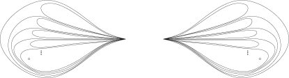
Figure 9: $W^{+}$ and $W^{-}$

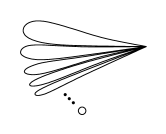
Figure 10: $S^{+}$

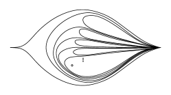
Figure 11: $V_{3}^{+}$

The infinitesimal edges of the train tracks described in this section are specified as follows. For each junction of $\mathbb{I}$, there is given one of the above symbols describing the basic configuration of infinitesimal edges. The junction is said to be type $\operatorname{BP}$, type $W^{+}$, type $W^{-}$, type $S^{+}$, type $V_{3}^{+}$ or type $V_{3}^{-}$ correspondingly. For each $2$-junction, there is in addition a symbol $L$ or $R$, specifying whether the loop(s) in the basic configuration are attached to the left or right switch in that junction. The $2$-junction is said to be type L or type R correspondingly.

In each $2$-junction not of type $V_{3}^{\pm}$, there is one additional infinitesimal edge, whose endpoints are the two switches on the boundary of the junction. This edge passes above (respectively below) all other infinitesimal edges in the junction if the junction is type R (respectively type L).

The reader seeking clarification as to how this notation is used can look ahead to Examples 8 and the accompanying figures.

There are two special cases: the finite order case $s=\operatorname{lhe}(m/n)$ (where each junction is of type $S^{+}$), and the NBT case $s=\operatorname{NBT}(m/n)$ (where each junction is of type $\operatorname{BP}$, and hence $\tau$ is finite). In all other cases, the invariant generalized train track contains junctions of types $W^{\pm}$ and $V_{3}^{\pm}$.

In all cases, it can be determined which $2$-junctions are type $L$ and which are type $R$ by applying the following simple algorithm. The idea is straightforward: the infinitesimal edges in junction $1$ are clearly attached to the right hand edge of that junction. This information is propagated around the orbit, with the type changing after each symbol $1$ (corresponding to a ‘flip’), and remaining unchanged after each symbol $0$.

Algorithm 1.

Let $s\in\mathcal{M}\mathcal{I}\mathcal{A}$ be a period $N$ kneading sequence, and let $\pi=\pi_{s}\in S_{N}$ denote the induced permutation on the points of the critical orbit of a corresponding unimodal map. Then the partition $\{2,\ldots,N-1\}=L\cup R$ is determined inductively as follows: $\pi(1)\in R$, and for each $r$ with $2\leq r\leq N-2$, $\pi^{r}(1)$ lies in the same set as $\pi^{r-1}(1)$ if $\pi^{r-1}(1)<\pi^{-1}(N)$, and in the other set if $\pi^{r-1}(1)>\pi^{-1}(N)$.

Example 7.

The easiest way to determine these sets is to write down the first $N$ symbols of $s$, and to place $L$s and $R$s above them. The $LR$ sequence starts with an $R$ at the third symbol, and changes after each $1$.

For example, let $s=(10011001011)^{\infty}$, so that $\pi=(1\,3\,7\,10\,2\,5\,9\,4\,8\,6\,11)$. Then Algorithm 1 gives

$$\begin{array}[]{ccccccccccc}11&1&3&7&10&2&5&9&4&8&6\\ &&R&R&L&R&R&R&L&L&R\\ 1&0&0&1&1&0&0&1&0&1&1.\end{array}$$

Thus $L=\{4,8,10\}$ and $R=\{2,3,5,6,7,9\}$.

The next result describes the invariant generalized train track corresponding to any periodic kneading sequence in $\mathcal{M}\mathcal{I}\mathcal{A}$.

Theorem 10.

Let $s\in\mathcal{M}\mathcal{I}\mathcal{A}$ be a periodic kneading sequence of period $N$ with height $m/n>0$. Then the invariant generalized train track corresponding to $s$ has infinitesimal edges as follows. Junction $i$ is of type $L$ or $R$ according as $i\in L$ or $i\in R$. The basic configurations of infinitesimal edges are:

1. If $s=\operatorname{lhe}(m/n)$, then all junctions are of type $S^{+}$.

2. If $s=\operatorname{NBT}(m/n)$, then all junctions are of type $\operatorname{BP}$.

3. Otherwise, let $\pi\in S_{N}$ denote the induced permutation on the points of the periodic critical orbit of a unimodal map with kneading sequence $s$, and let $\epsilon\in\{+,-\}$ be given by $\epsilon=+$ if $\pi^{-1}(N)\in R$, and $\epsilon=-$ if $\pi^{-1}(N)\in L$. Then for $0\leq r\leq N-1$, the junction $\pi^{r}(N)$ is of type $W^{\epsilon}$ if $r\leq n+1$, and of type $V_{3}^{\epsilon}$ if $r>n+1$.

The proof is delayed until some explanatory examples have been presented.

Examples 8.

The three examples correspond to the three cases of Theorem 10.

1. Let $s=(101)^{\infty}=\operatorname{lhe}(1/3)$, so that $\pi=(1\,2\,3)$. Algorithm 1 gives

   $$\begin{array}[]{ccc}3&1&2\\ &&R\\ 1&0&1\end{array}$$

   Thus the invariant generalized train track is described by

   $$(S^{+}\,\,;\,\,S^{+},R\,\,;\,\,S^{+})$$

   (see Figure 12: note that the infinitesimal edge with endpoints the left and right switches in junction 2 passes above the other infinitesimal edges in the junction, since the junction is of type R. In this and subsequent figures, the punctures have been labelled to clarify the dynamics.)

   \psfrag{f}{$\scriptstyle{\phi}$}\psfrag{1}{$\scriptstyle{1}$}\psfrag{2}{$\scriptstyle{2}$}\psfrag{3}{$\scriptstyle{3}$}\includegraphics[width=260.17464pt]{101itt2}

   Figure 12: The generalized train track corresponding to $s=\operatorname{lhe}(1/3)$ and its image

2. Let $s=(10011)^{\infty}=\operatorname{NBT}(1/3)$, so $\pi=(1\,2\,4\,3\,5)$. Algorithm 1 gives

   $$\begin{array}[]{ccccc}5&1&2&4&3\\ &&R&R&L\\ 1&0&0&1&1\end{array}$$

   Thus the invariant generalized train track is described by

   $$(\operatorname{BP}\,\,;\,\,\operatorname{BP},R\,\,;\,\,\operatorname{BP},L\,\,;\,\,\operatorname{BP},R\,\,;\,\,\operatorname{BP})$$

   (see Figure 13).

   \psfrag{f}{$\scriptstyle{\phi}$}\psfrag{1}{$\scriptstyle{1}$}\psfrag{2}{$\scriptstyle{2}$}\psfrag{3}{$\scriptstyle{3}$}\psfrag{4}{$\scriptstyle{4}$}\psfrag{5}{$\scriptstyle{5}$}\includegraphics[width=346.89731pt]{10010tt2}

   Figure 13: The generalized train track corresponding to $s=\operatorname{NBT}(1/3)$ and its image

3. Let $s=(1001011)^{\infty}$, so $q(s)=1/3$ and $\pi=(1\,3\,6\,2\,5\,4\,7)$. Algorithm 1 gives

   $$\begin{array}[]{ccccccc}7&1&3&6&2&5&4\\ &&R&R&L&L&R\\ 1&0&0&1&0&1&1\end{array}$$

   Thus $\epsilon=+$, since $\pi^{-1}(7)=4\in R$. The junctions $\pi^{r}(7)$ with $0\leq r\leq 4$ are $7$, $1$, $3$, $6$, and $2$, so these junctions are of type $W^{+}$, while junctions $5$ and $4$ are of type $V_{3}^{+}$. Thus the invariant generalized train track is described by

   $$(W^{+}\,\,;\,\,W^{+},L\,\,;\,\,W^{+},R\,\,;\,\,V_{3}^{+},R\,\,;\,\,V_{3}^{+},L\,\,;\,\,W^{+},R\,\,;\,\,W^{+})$$

   (see Figure 14).

   \psfrag{f}{$\scriptstyle{\phi}$}\psfrag{1}{$\scriptstyle{1}$}\psfrag{2}{$\scriptstyle{2}$}\psfrag{3}{$\scriptstyle{3}$}\psfrag{4}{$\scriptstyle{4}$}\psfrag{5}{$\scriptstyle{5}$}\psfrag{6}{$\scriptstyle{6}$}\psfrag{7}{$\scriptstyle{7}$}\includegraphics[width=411.93767pt,height=142.26378pt]{1011tt2}

   Figure 14: The generalized train track corresponding to $s=(1001011)^{\infty}$ and its image

Proof of Theorem 10.

Let $\tau$ be the invariant generalized train track, as constructed using the algorithm of Theorem 1. Let $A\subseteq\{2,\ldots,N-1\}$ (respectively $B\subseteq\{2,\ldots,N-1\}$) be the set of $2$-junctions which contain an infinitesimal edge of $\tau$ joining the two switches in the junction and passing above (respectively below) the puncture. There are two ways such edges can arise during the construction. First, as images of real edges: this requires that $r\in A$ (respectively $r\in B$) if $r\geq\pi(1)$ and $\pi^{-1}(r)<\pi^{-1}(N)$ (respectively $r\geq\pi(1)$ and $\pi^{-1}(r)>\pi^{-1}(N)$). Second, as images of other such infinitesimal edges: this requires that if $\pi^{-1}(r)<\pi^{-1}(N)$ then $r$ lies in $A$ (respectively $B$) if $\pi^{-1}(r)$ lies in $A$ (respectively $B$); while if $\pi^{-1}(r)>\pi^{-1}(N)$ then $r$ lies in $B$ (respectively $A$) if $\pi^{-1}(r)$ lies in $A$ (respectively $B$).

To express this symbolically, partition $\{1,\ldots,N\}=O\cup I$, with $r\in O$ if $r<\pi^{-1}(N)$ (ie, if $r$ corresponds to the symbol $0$), and $r\in I$ otherwise. Then $A$ and $B$ are the smallest subsets of $\{2,\ldots,N-1\}$ such that

1. If $r\geq\pi(1)$, then $r\in A$ if $\pi^{-1}(r)\in O$, and $r\in B$ if $\pi^{-1}(r)\in I$.

2. If $\pi^{-1}(r)\in O$ then $r\in A$ if $\pi^{-1}(r)\in A$, and $r\in B$ if $\pi^{-1}(r)\in B$. If $\pi^{-1}(r)\in I$ then $r\in B$ if $\pi^{-1}(r)\in A$, and $r\in A$ if $\pi^{-1}(r)\in B$.

By condition ii), $A\cap B$ is a final segment of the sequence $(\pi^{j}(1))_{j=1}^{N-2}$. By conditions i) and ii), the least $j$ such that $\pi^{j}(1)\in A\cap B$ is the least $j$ with $\pi^{j}(1)>\pi(1)$ and $\pi^{j-1}(1)\in B$. The main step of the proof is to establish that this least $j$ is equal to $n+1$. In particular, by Lemma 5, $A\cap B=\emptyset$ if and only if either $s=\operatorname{lhe}(m/n)$ or $s=\operatorname{NBT}(m/n)$.

By Lemma 5, either $s=\operatorname{lhe}(m/n)$ or $s=c_{m/n}d$ for some $d\in\{0,1\}^{\mathbb{N}}$. Assume that the latter holds: the proof that $A\cap B=\emptyset$ in the former case is similar. Now since $1\in O$, condition i) gives $\pi(1)\in A$, and the assignments to $A$ and $B$ given by condition ii) are as follows:

$$s=\begin{array}[]{ccccccccccccc}&A&A&B&A&A&B&&A&B&A&A&\\ 1&0^{\kappa_{1}}&1&1&0^{\kappa_{2}}&1&1&\ldots&1&1&0^{\kappa_{m}}&1&d\end{array}$$

Using $i(\pi(1))=0^{\kappa_{1}-1}1^{2}0^{\kappa_{2}}1^{2}\ldots 1^{2}0^{\kappa_{m}}1d=\sigma^{2}(s)$ and applying Lemma 7 gives $j\geq n+1$. Since the first symbol of $d$ corresponds to an element of $B$, it only remains to show that $\sigma(d)\succeq\sigma^{2}(s)$. This is given by Lemma 8.

Notice that for $r\not\in A\cap B$, comparing condition ii) with Algorithm 1 gives that $r\in A$ if and only if $r\in R$.

Now consider how loops can arise during the construction of $\tau$. Again, there are two ways. First, as the image of an infinitesimal edge joining the two switches of junction $\pi^{-1}(N)$: this gives rise to a homotopically trivial bubble in junction $N$ (respectively a loop containing the puncture in junction $N$) if the edge passes above (respectively below) the puncture in junction $\pi^{-1}(N)$. Second, as the image of another loop.

If $s=\operatorname{NBT}(m/n)$, ie,

$$s=\begin{array}[]{cccccccccccccc}&A&A&B&A&A&B&&A&B&A&A&B&\\ 1&0^{\kappa_{1}}&1&1&0^{\kappa_{2}}&1&1&\ldots&1&1&0^{\kappa_{m}}&1&1&\ldots,\end{array}$$

then any infinitesimal edge joining the switches of junction $\pi^{-1}(N)$ passes below the puncture, and hence gives rise to a loop in junction $N$ which contains the puncture. Statement b) follows easily. Similarly, if $s=\operatorname{lhe}(m/n)$, ie,

$$s=\begin{array}[]{ccccccccccccc}&A&A&B&A&A&B&&A&B&A&A&\\ 1&0^{\kappa_{1}}&1&1&0^{\kappa_{2}}&1&1&\ldots&1&1&0^{\kappa_{m}-1}&1&\ldots,\end{array}$$

then any infinitesimal edge joining the switches of junction $\pi^{-1}(N)$ passes above the puncture, and hence gives rise to a homotopically trivial bubble in junction $N$. Statement a) follows.

In any other case, $\pi^{-1}(N)\in A\cap B$, so that both homotopically trivial bubbles and homotopically non-trivial loops are created in junction $N$, leading under iteration of the construction to a configuration of infinitesimal edges of type $W$ in each junction. The orientation of these infinitesimal edges bubbles depends on whether $\pi^{-1}(N)\in R$ or $\pi^{-1}(N)\in L$ (which determines whether a new homotopically trivial bubble arises below or above the existing loops in junction $N$ during the construction). Junction $r$ is of type $V_{3}^{\pm}$ if $r\in A\cap B$, but of type $W^{\pm}$ if $r$ is in only one of $A$ and $B$. Statement c) follows. ∎

6.2 The preperiodic case

The preperiodic case is somewhat more complicated than the periodic case, though there are no new ideas introduced: as such, the treatment is more informal and some of the details are omitted. The most substantial modifications arising because the critical point is not periodic are:

1. There is a unique loop which arises during the construction as the image of an infinitesimal edge which is not a loop, and this loop is a homotopically trivial bubble. All other loops are images of this one, and hence all loops are homotopically trivial bubbles.

2. Only finitely many infinitesimal edges occur in those junctions corresponding to the strictly preperiodic part of the orbit of the critical point.

3. The parity of the periodic part of the kneading sequence plays an important role. If there are an odd number of $1$s, then there is a flip each time around the periodic orbit, and hence bubbles are attached to both the left and right switches of $2$-junctions.

4. In the periodic case, the configuration of infinitesimal edges changes (from $W$ to $V_{3}$) at a point in the orbit given by the denominator of the height. In the preperiodic case, separate cases arise according as this point lies in the preperiodic or periodic part of the orbit.

The basic configurations of infinitesimal edges are entirely different from the periodic case. There are two distinct types: those which arise in junctions corresponding to the preperiodic part of the orbit ($B$ and $V_{0}$), which contain only finitely many infinitesimal edges and have no associated puncture; and those which arise in periodic junctions, which contain infinitely many infinitesimal edges and have an associated puncture. The configurations are:

$B$

A single (homotopically trivial) bubble.

$V_{0}$

A bigon containing a single bubble, as depicted in Figure 15.

$S^{-}$

The mirror image of $S^{+}$.

$V_{1}$

A decorated bigon as depicted in Figure 16. There are two versions, $V_{1}^{+}$ and $V_{1}^{-}$, which are mirror images of each other. In addition, an additional external bubble may be present in the position indicated in Figure 18. In this case, the configuration is denoted $V_{1}^{\pm}\,B$.

$V_{2}$

A decorated bigon as depicted in Figure 17. There are two versions, $V_{2}^{+}$ and $V_{2}^{-}$: $V_{2}^{+}$ is the mirror image of $V_{2}^{-}$. In addition, there may be two additional external bubbles in the positions indicated in Figure 18. In this case, the configuration is denoted $V_{2}^{\pm}\,B^{2}$.

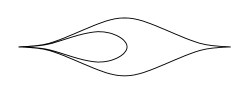
Figure 15: $V_{0}$

\psfrag{v1-}{$\scriptstyle{V_{1}^{-}}$}\psfrag{v1+}{$\scriptstyle{V_{1}^{+}}$}\includegraphics[width=260.17464pt]{v1}

Figure 16: $V_{1}^{-}$ and $V_{1}^{+}$

\psfrag{v2-}{$\scriptstyle{V_{2}^{-}}$}\includegraphics[width=130.08731pt]{v2}

Figure 17: $V_{2}^{-}$

Figure 18: Extra bubbles: the configurations $V_{1}^{+}\,B$ and $V_{2}^{-}\,B^{2}$

For each junction of $\mathbb{I}$, one of the above symbols is given describing the basic configuration of infinitesimal edges: the junction is said to be type $V_{0}$, type $V_{1}^{-}$, type $V_{2}^{+}\,B^{2}$, etc. Each $2$-junction which is not of type $V_{2}$ is either type $L$ or type $R$, according as the bubbles are attached to the left or right switch of the junction. For each $2$-junction of type $B$ or $S^{-}$, there is one additional infinitesimal edge, whose endpoints are the two switches on the boundary of the junction. This edge passes above (respectively below) all other infinitesimal edges in the junction if the junction is type $R$ (respectively type $L$).

Throughout this subsection $s$ denotes a strictly preperiodic kneading sequence, written $s=vw^{\infty}$, where $v$ is taken to be as short a word as possible (so the final symbol of $v$ is not equal to the final symbol of $w$). The lengths of $v$ and $w$ will be denoted $k$ and $l$ respectively (so $k,l\geq 1$), and the size of the orbit of $s$ under the shift map is denoted $N=k+l$. The $N$ points of this orbit are labelled with the integers $1$ through $N$ according to their relative unimodal ordering (so point $r$ lies in junction $r$). The shift map $\sigma$ thus induces a map $\rho\co\{1,\ldots,N\}\includegraphics[height=7.22743pt]{backarr.eps}$. Note that $\rho$ is not a permutation: the point $N$ (corresponding to the first symbol of $s$) has no preimage, and one point (corresponding to the first symbol of $w$) has two preimages.

The following algorithm is the analogue of Algorithm 1 for the preperiodic case. Notice that $L\cup R$ need not be a partition of $\{2,\ldots,N-1\}$ (reflecting the possibility that the word $w$ may be odd): if $r\in L\cap R$, then bubbles are attached to both switches in junction $r$ (configuration $V_{2}$).

Algorithm 2.

The subsets $L$ and $R$ of $\{2,\ldots,N-1\}$ are determined inductively as follows. Let $\rho^{2}(N)\in R$, and for each $r$ with $3\leq r\leq N+l-1$, let $\rho^{r}(N)$ lie in the same set as $\rho^{r-1}(N)$ if $s_{r-1}=0$, and in the other set if $s_{r-1}=1$.

If $w$ is an even word, then the final $l$ steps in this algorithm are unnecessary, and $L\cap R=\emptyset$.

Examples 9.

1. Let $s=1000(101)^{\infty}$. Then $v=1000$, $w=101$, and

   $$\rho=\left(\begin{array}[]{ccccccc}1&2&3&4&5&6&7\\ 2&4&5&6&6&3&1\end{array}\right)$$

   (ie, the $\rho$-orbit of $7$ is $7124(635)^{\infty}$). Thus

   $$\begin{array}[]{ccccccccl}7&1&2&4&&6&3&5&\\ &&R&R&&R&L&L&,\\ 1&0&0&0&&1&0&1&\end{array}$$

   and so $L=\{3,5\}$ and $R=\{2,4,6\}$.

2. Let $s=100101(10)^{\infty}$. Then $v=100101$, $w=10$, and

   $$\rho=\left(\begin{array}[]{cccccccc}1&2&3&4&5&6&7&8\\ 4&5&6&7&6&3&2&1\end{array}\right)$$

   (ie, the $\rho$-orbit of $8$ is $814725(63)^{\infty}$). Thus

   $$\begin{array}[]{ccccccccccccl}8&1&4&7&2&5&&6&3&&6&3&\\ &&R&R&L&L&&R&L&&L&R&,\\ 1&0&0&1&0&1&&1&0&&1&0&\end{array}$$

   and so $L=\{2,3,5,6\}$ and $R=\{3,4,6,7\}$. Note that since $w$ is odd, the two repeating points $3$ and $6$ of the orbit lie in both $L$ and $R$.

For preperiodic kneading sequences, there is only one special case: that in which $s=\operatorname{rhe}(m/n)$.

Theorem 11.

Let $s=vw^{\infty}\in\mathcal{M}\mathcal{I}\mathcal{A}$ be a strictly preperiodic kneading sequence of height $m/n>0$. Let $k$ and $l$ be the lengths of $v$ and $w$ (chosen as small as possible). Let $\rho$ be the induced map on $\{1,\ldots,N=k+l\}$. Then the invariant generalized train track corresponding to $s$ has infinitesimal edges as follows. If $i\in L\setminus R$ (respectively $i\in R\setminus L$) then junction $i$ is of type $L$ (respectively $R$). The basic configurations of infinitesimal edges are:

1. If $s=\operatorname{rhe}(m/n)$, then the junction $\rho^{r}(N)$ is of type $B$ for $0\leq r<k$, and of type $S^{-}$ for $k\leq r<N$.

2. Otherwise, let $\epsilon\in\{+,-\}$ be given by $\epsilon=+$ if $\rho^{k-1}(N)\in R$, and $\epsilon=-$ if $\rho^{k-1}(N)\in L$. Then for each $r$ with $0\leq r<N$:

   1. If $r\leq n+1$, then junction $\rho^{r}(N)$ is of type

      • $B$, if $r\leq k$.

      • $V_{1}^{\epsilon}\,B$ or $V_{2}^{\epsilon}\,B^{2}$ (according as $w$ is even or odd), if $r>k$.

   2. If $r>n+1$, then junction $\rho^{r}(N)$ is of type

      • $V_{0}$, if $r\leq k$.

      • $V_{1}^{\epsilon}$ or $V_{2}^{\epsilon}$ (according as $w$ is even or odd), if $r>k$.

Examples 10.

The first example illustrates the case $s=\operatorname{rhe}(m/n)$. The other two examples show the two possibilities $w$ even and $w$ odd.

1. Let $q=1/3$ and $s=\operatorname{rhe}(q)$ so $s=1001(101)^{\infty}=10(011)^{\infty}$. Thus $v=10$, $w=011$, and

   $$\rho=\left(\begin{array}[]{ccccc}1&2&3&4&5\\ 2&3&4&2&1\end{array}\right)$$

   (ie, the $\rho$-orbit of $5$ is $51(234)^{\infty}$). Thus

   $$\begin{array}[]{ccccccl}5&1&&2&3&4&\\ &&&R&R&L&,\\ 1&0&&0&1&1&\end{array}$$

   and so $R=\{2,3\}$ and $L=\{4\}$.

   Since $k=2$ and $l=3$, junctions $N=5$ and $\rho(N)=1$ are of type $B$, while the other junctions are of type $S^{-}$.

   Thus the invariant generalized train track is described by

   $$(B\,\,;\,\,S^{-},R\,\,;\,\,S^{-},R\,\,;\,\,S^{-},L\,\,;\,\,B)$$

   (see figure 19: here all junctions have been labelled to clarify the dynamics).

2. Let $s=\overset{7}{1}\overset{1}{0}\overset{2}{0}\overset{4}{0}(\overset{6}{1}\overset{3}{0}\overset{5}{1})^{\infty}$. Then $L=\{3,5\}$ and $R=\{2,4,6\}$ (see Example 9 a)).

   Since $k=4$ and $l=3$, $\rho^{k-1}(N)=\rho^{3}(7)=4\in R$, and hence $\epsilon=+$. $s$ has height $q(s)=1/4$, so $n=4$. Thus junctions $N=7$, $\rho(N)=1$, $\rho^{2}(N)=2$, and $\rho^{3}(N)=4$ are of type $B$; junctions $\rho^{4}(N)=6$ and $\rho^{5}(N)=3$ are of type $V_{1}^{+}\,B$; and junction $\rho^{6}(N)=5$ is of type $V_{1}^{+}$.

   Thus the invariant generalized train track is described by

   $$(B\,\,;\,\,B,R\,\,;\,\,V_{1}^{+}\,B,L\,\,;\,\,B,R\,\,;\,\,V_{1}^{+},L\,\,;\,\,V_{1}^{+}\,B,R\,\,;\,\,B)$$

   (see Figure 20).

3. Let $s=\overset{8}{1}\overset{1}{0}\overset{4}{0}\overset{7}{1}\overset{2}{0}\overset{5}{1}(\overset{6}{1}\overset{3}{0})^{\infty}$. Then $L=\{2,3,5,6\}$ and $R=\{3,4,6,7\}$ (see Example 9 b)).

   Since $k=6$ and $l=2$, $\rho^{k-1}(N)=\rho^{5}(8)=5\in L$, and hence $\epsilon=-$. $s$ has height $q(s)=1/3$, so $n=3$. Thus junctions $N=8$, $\rho(N)=1$, $\rho^{2}(N)=4$, $\rho^{3}(N)=7$, and $\rho^{4}(N)=2$ are of type $B$; junction $\rho^{5}(N)=5$ is of type $V_{0}$; and junctions $\rho^{6}(N)=6$ and $\rho^{7}(N)=3$ are of type $V_{2}^{-}$.

   Thus the invariant generalized train track is described by

   $$(B\,\,;\,\,B,L\,\,;\,\,V_{2}^{-}\,\,;\,\,B,R\,\,;\,\,V_{0},L\,\,;\,\,V_{2}^{-}\,\,;\,\,B,R\,\,;\,\,B)$$

   (see Figure 21).

\psfrag{f}{$\scriptstyle{\phi}$}\psfrag{1}{$\scriptstyle{1}$}\psfrag{2}{$\scriptstyle{2}$}\psfrag{3}{$\scriptstyle{3}$}\psfrag{4}{$\scriptstyle{4}$}\psfrag{5}{$\scriptstyle{5}$}\includegraphics[width=346.89731pt]{b011itt2}

Figure 19: The generalized train track corresponding to $s=\operatorname{rhe}(1/3)$ and its image

\psfrag{f}{$\scriptstyle{\phi}$}\psfrag{1}{$\scriptstyle{1}$}\psfrag{2}{$\scriptstyle{2}$}\psfrag{3}{$\scriptstyle{3}$}\psfrag{4}{$\scriptstyle{4}$}\psfrag{5}{$\scriptstyle{5}$}\psfrag{6}{$\scriptstyle{6}$}\psfrag{7}{$\scriptstyle{7}$}\includegraphics[width=411.93767pt]{b101tt2}

Figure 20: The generalized train track corresponding to $s=1000(101)^{\infty}$ and its image

\psfrag{f}{$\scriptstyle{\phi}$}\psfrag{1}{$\scriptstyle{1}$}\psfrag{2}{$\scriptstyle{2}$}\psfrag{3}{$\scriptstyle{3}$}\psfrag{4}{$\scriptstyle{4}$}\psfrag{5}{$\scriptstyle{5}$}\psfrag{6}{$\scriptstyle{6}$}\psfrag{7}{$\scriptstyle{7}$}\psfrag{8}{$\scriptstyle{8}$}\includegraphics[width=411.93767pt]{b10tt2}

Figure 21: The generalized train track corresponding to $s=100101(10)^{\infty}$ and its image

Sketch proof of Theorem 11.

The proof is very similar to that of Theorem 10. Defining sets $A$ and $B$ as there, and noting that $s=c_{m/n}d$ for some $d\in\{0,1\}^{\mathbb{N}}$, the same analysis shows that $A\cap B=\emptyset$ if and only if $s=\operatorname{rhe}(m/n)$, and in all other cases $A\cap B=\{\rho^{j}(N)\,:\,n+2\leq j\leq N-1\}$. This is again the essential part of the proof.

When $s=\operatorname{rhe}(m/n)$, it is then straightforward to check case a). In other cases, it is immediate that for $r\leq k$ (ie, in the preperiodic part of the orbit) $r$ has type $V_{0}$ if $r\in A\cap B$, and type $B$ otherwise.

All of the bubbles arise in the construction as images of the bubble in junction $N$ (which itself is created as the image of part of a real edge). In particular, they are all homotopically trivial. The combinatorics of the different cases can be checked routinely. ∎

7 Unimodal generalized pseudo-Anosov maps

In this section the construction of generalized pseudo-Anosov maps starting from the invariant train tracks of Section 6 is described.

7.1 Preliminaries

Let $F\co(S^{2},\mathbb{I},A)\includegraphics[height=7.22743pt]{backarr.eps}$ be a unimodal MIA thick interval map, where $A$ is the set of attracting periodic points of $F$. Let $f\co I\includegraphics[height=7.22743pt]{backarr.eps}$ be the quotient unimodal map, and $\phi\co\tau\includegraphics[height=7.22743pt]{backarr.eps}$ be the associated generalized train track map. Let $e_{1},e_{2},\ldots,e_{N-1}$ denote the real edges of $\tau$, and $e_{N},e_{N+1},\ldots$ denote the infinitesimal edges. Define the transition matrix $M=(m_{ij})$ by

$$m_{ij}=\mbox{number of times\ }\phi(e_{j})\mbox{\ crosses\ }e_{i}.$$

Thus $M$ is an infinite matrix, unless $\kappa(F)=\operatorname{NBT}(m/n)$ for some $m/n\in(0,1/2)$.

From the construction of the invariant generalized train track in Section 6, it is immediate that each $\phi(e_{j})$ is a finite length edge path; that each $e_{i}$ is contained in the edge path $\phi(e_{j})$ for only finitely many $j$; and that each infinitesimal edge is mapped by $\phi$ homeomorphically onto an infinitesimal edge. These observations yield the following facts about the strucure of the transition matrix:

1. $M$ is of the form

   $$M=\left(\begin{array}[]{cc}A&0\\ B&\Pi\end{array}\right),$$

   where $A$ is an $(N-1)\times(N-1)$ matrix recording transitions between real edges, $\Pi$ records transitions between infinitesimal edges, and $B$ records transitions from real to infinitesimal edges.

2. All entries of $\Pi$ are either $0$ or $1$. Each column of $\Pi$ has exactly one non-zero entry, and each row has only finitely many non-zero entries.

3. $B$ has only finitely many non-zero entries in each column.

In particular, if $M$ is regarded as an operator acting on $l^{1}$, then $M$ is bounded with $\|M\|_{1}\leq\max_{j}\left\{\sum_{i}|m_{ij}|\right\}<\infty$. Let $\lambda$ be the Perron-Frobenius eigenvalue of $A$, and $Y\in\mathbb{R}^{N-1}$ the associated positive eigenvector. Then $Y$ can be extended to a positive eigenvector $y=(Y\,Y^{\prime})\in l^{1}$ of $M$, called the Perron-Frobenius eigenvector of $M$, by setting

$$Y^{\prime}=\frac{1}{\lambda}(B+\frac{1}{\lambda}\Pi B+\frac{1}{\lambda^{2}}\Pi^{2}B+\ldots)Y.$$

Note that $\|\Pi\|_{1}\leq 1$ so that the series above converges in $l^{1}$, implying that $y=(Y\,Y^{\prime})\in l^{1}$. Note also that the matrices $\Pi^{k}B$ represent transitions from a real edge to an infinitesimal edge under $\phi$, and then to another infinitesimal edge under a further $k$ iterations of $\phi$. By the construction of $\tau$ described in the proof of Theorem 1, every infinitesimal edge of $\tau$ is the image, under some iterate of $\phi$, of some infinitesimal edge of $F_{*}(\tau(\emptyset))$, and each of these infinitesimal edges is crossed by $\phi(e)$ for some real edge $e$. Thus for all $i\geq 1$ there exists $k\geq 1$ such that row $i$ of $\Pi^{k}B$ is non-zero. Since $Y$ is a strictly positive vector, this establishes that every entry of $Y^{\prime}$ is also positive.

Definition 15.

A sequence $(y_{i})$ of positive real numbers is said to satisfy the switch conditions for $\tau$ if, for each switch $q$ of $\tau$,

$$y_{i_{0}}=\sum y_{i}+2\sum y_{j},$$

where $e_{i_{0}}$ is the real edge with endpoint $q$, and the first and second sums range over the sets of indices of infinitesimal edges having one and both endpoints at $q$ respectively.

The proof of the following lemma is essentially the same as that of the corresponding fact for finite matrices in Section 3.4 of [2].

Lemma 12.

Let the transition matrix $M$ of $\phi\co\tau\includegraphics[height=7.22743pt]{backarr.eps}$ have Perron-Frobenius eigenvector $y=(y_{1}\,y_{2}\,\ldots)$. Then $y$ satisfies the switch conditions for $\tau$.

Proof.

For $r,s,k\geq 1$ denote by $m^{(k)}_{rs}$ the number of times that $\phi^{k}(e_{s})$ crosses $e_{r}$. Thus $m^{(k)}_{rs}=(M^{k})_{rs}$. The fact that $y$ is an eigenvector of $M^{k}$ with eigenvalue $\lambda^{k}$ thus gives that for any $k$ and any $r$,

$$y_{r}=\frac{1}{\lambda^{k}}\sum_{s=1}^{\infty}m^{(k)}_{rs}y_{s}.$$

Now if $q$ is a switch of $\tau$ which is an endpoint of the real edge $e_{i_{0}}$, and if $I$ and $J$ are the sets of indices of infinitesimal edges having one and two endpoints at $q$ respectively, then for any $s$,

$$\left(\sum_{i\in I}m^{(k)}_{is}+2\sum_{j\in J}m^{(k)}_{js}\right)-2\leq m^{(k)}_{i_{0}s}\leq\left(\sum_{i\in I}m^{(k)}_{is}+2\sum_{j\in J}m^{(k)}_{js}\right)+2.$$

This is because, except at its endpoints, $\phi^{k}(e_{s})$ must cross both $e_{i_{0}}$ and an edge indexed in $I\cup J$ each time it intersects $q$. Multiplying by $y_{s}$, summing over $s$, and dividing by $\lambda^{k}$ gives

$$\left|\sum_{i\in I}y_{i}+2\sum_{j\in J}y_{j}-y_{i_{0}}\right|\leq\frac{2\sum_{s=1}^{\infty}y_{s}}{\lambda^{k}},$$

which gives the result on letting $k\to\infty$. ∎

Now let $X\in\mathbb{R}^{N-1}$ be an eigenvector of $A^{T}$ associated to the Perron-Frobenius eigenvalue $\lambda$. If $x=(X\,X^{\prime})\in l^{\infty}$ is a completion of $X$ to an eigenvector of the adjoint $M^{*}$ then $X^{\prime}=0$, since it satisfies the equation $(\lambda I-\Pi^{*})X^{\prime}=0$, and $\|\Pi^{*}\|_{\infty}\leq 1<\lambda$.

7.2 The construction

The construction will be illustrated by means of a running example, where $F\co(S^{2},\mathbb{I},A)\includegraphics[height=7.22743pt]{backarr.eps}$ is a unimodal MIA thick interval map with $\kappa(F)=(1001011)^{\infty}$, as depicted in Figure 4. The associated generalized train track map $\phi\co\tau\includegraphics[height=7.22743pt]{backarr.eps}$ is depicted in Figure 14.

Let $x=(x_{1},x_{2},\ldots,x_{N-1},0,0,\ldots)$ and $y=(y_{1},y_{2},\ldots)$ be the eigenvectors of $M^{*}$ and $M$ associated to the Perron-Frobenius eigenvalue $\lambda$ of $A$ as described above. For definiteness these vectors are scaled so that $\|x\|_{2}=1$ and $\sum x_{i}y_{i}=1$, although this normalization can be chosen arbitrarily. In the running example, to $3$ decimal places:

$$A=\left(\begin{array}[]{cccccc}0&0&0&0&0&1\\ 0&0&0&0&1&0\\ 1&0&0&0&1&0\\ 1&0&0&1&0&0\\ 0&1&0&1&0&0\\ 0&0&1&1&0&0\end{array}\right)\!,\qua\lambda=1.686,\qua X=\left(\begin{array}[]{c}0.543\\ 0.104\\ 0.191\\ 0.724\\ 0.175\\ 0.322\end{array}\right)\!,\qua Y=\left(\begin{array}[]{c}0.368\\ 0.291\\ 0.509\\ 0.536\\ 0.490\\ 0.620\end{array}\right)$$

Associate a Euclidean rectangle $R_{i}$ of width $x_{i}$ and height $y_{i}$, foliated by horizontal and vertical line segments, to each real edge $e_{i}$ of $\tau$. The idea of the construction is as follows: a topological sphere $S$ is constructed by identifying the vertical sides of these rectangles in the manner dictated by the infinitesimal edges of $\tau$ and then identifying the horizontal sides in such a way that the train track map $\phi$ defines a homeomorphism $\Phi\co S\includegraphics[height=7.22743pt]{backarr.eps}$. The foliations of the rectangles project to singular foliations of $S$ with transverse measures induced by the Euclidean metric: these foliations are preserved by $\Phi$, the horizontal and vertical foliations being stretched and contracted by factors $\lambda$ and $1/\lambda$ respectively, so that $\Phi$ is a generalized pseudo-Anosov map.

When $\tau$ is finite (ie, when $\kappa(F)=\operatorname{NBT}(m/n)$ for some $m/n$), this construction is identical to that of [2], and produces a pseudo-Anosov homeomorphism. When $\tau$ is infinite, however, the construction involves infinitely many sets of identifications, and it is therefore necessary to describe them carefully and to justify that the quotient space is a sphere. The tool used to do this is Moore’s theorem [16] on monotone upper semi-continuous (m.u.s.c.) decompositions of the sphere.

Definitions 16.

A partition or decomposition ${\mathcal{G}}$ of a topological space into compact sets is upper semi-continuous if for every decomposition element $\zeta\in{\mathcal{G}}$ and every open set $U\supset\zeta$, there exists an open set $V\subset U$ with $\zeta\subset V$ such that every $\zeta^{\prime}\in{\mathcal{G}}$ with $\zeta^{\prime}\cap V\neq\emptyset$ has $\zeta^{\prime}\subset U$. The decomposition is monotone if its elements are connected.

The proof of the following lemma is routine.

Lemma 13.

A decomposition ${\mathcal{G}}$ of a compact metric space $X$ is upper semi-continuous if and only if whenever $x_{n}\to x$ and $y_{n}\to y$ are convergent sequences in $X$ such that $x_{n}$ and $y_{n}$ belong to the same element of ${\mathcal{G}}$ for all $n$, then $x$ and $y$ belong to the same element of ${\mathcal{G}}$.∎

Theorem 14 (Moore).

Let ${\mathcal{G}}$ be a monotone upper semi-continuous decomposition of a topological sphere $S$ such that no decomposition element separates $S$. Then the quotient space obtained by collapsing each decomposition element to a point is a topological sphere.

The side identifications will be realized by arc bands with which m.u.s.c. decompositions of the sphere will be constructed. These arc bands are of two types:

• A rectangular arc band $\eta$ of size $y$ is the image of an embedding $\psi\co[0,1]\times[0,y]\to S^{2}$ which restricts to a Euclidean isometry on $\{0\}\times[0,y]$ and on $\{1\}\times[0,y]$, foliated by the leaves $\psi([0,1]\times\{t\})$ for $0\leq t\leq y$. The vertices of $\eta$ are the points $\psi(0,0)$, $\psi(0,y)$, $\psi(1,0)$, and $\psi(1,y)$.

• A semi-circular arc band $\eta$ of size $y$ is the image of an embedding

  $$\psi\co\{(s,t)\in\mathbb{R}^{2}\,:\,t\in[-y,y],\,s\in[0,\sqrt{y^{2}-t^{2}}]\}\to S^{2}$$

  which restricts to a Euclidean isometry on $\{0\}\times[-y,y]$, foliated by the leaves

  $$\psi\left(\{(\sqrt{r^{2}-t^{2}},t)\,:\,t\in[-r,r]\}\right)$$

  for $0\leq r\leq y$. The vertices of $\eta$ are the points $\psi(0,-y)$ and $\psi(0,y)$, and its centre is $\psi(0,0)$.

The decomposition of an arc band $\eta$ into the leaves of its foliation is clearly m.u.s.c.

7.2.1 Identifications of vertical sides

Place isometric copies of the rectangles $R_{i}$ in $S^{2}$ along the real edges of $\tau$, as illustrated for the running example in Figure 22.

\psfrag{R1}{$\scriptstyle{R_{1}}$}\psfrag{R2}{$\scriptstyle{R_{2}}$}\psfrag{R3}{$\scriptstyle{R_{3}}$}\psfrag{R4}{$\scriptstyle{R_{4}}$}\psfrag{R5}{$\scriptstyle{R_{5}}$}\psfrag{R6}{$\scriptstyle{R_{6}}$}\includegraphics[width=346.89731pt]{constr1}

Figure 22: The rectangles $R_{i}$ placed along the real edges of $\tau$

For each infinitesimal edge $e_{i}$ of $\tau$, place an arc band $\eta_{i}$ of size $y_{i}$ in $S^{2}$, joining the segments of length $y_{i}$ on the vertical sides of the rectangles corresponding to the real edges adjacent to the endpoints of $e_{i}$. If $e_{i}$ is a bubble then these segments are adjacent on the same vertical side of the same rectangle, and $\eta_{i}$ is a semi-circular arc band; otherwise, $\eta_{i}$ is rectangular. The arc bands are placed on the sphere in the configuration dictated by $\tau$, and are chosen to be mutually disjoint except possibly at their vertices. By Lemma 12, the arc bands incident on any given vertical side of a rectangle precisely cover that side. When there are infinitely many infinitesimal edges in a given junction, then some care is needed in the placement of these arc bands to ensure that Moore’s theorem can be applied (despite the fact that the arc bands only serve to indicate how the vertical sides of the rectangles should be identified, and from this point of view the details of their placement is irrelevant).

$S^{\pm}$

Choose the semi-circular arc bands with diameters converging to $0$, which is possible since their sizes converge to $0$.

$W^{\pm}$, $V_{3}^{\pm}$

Choose the semi-circular arc bands with diameters converging to $0$. It is then possible to choose the rectangular arc bands so that their diameters converge to $0$ (see Figure 23 for the arc bands in the junction between $R_{3}$ and $R_{4}$ in the running example). Note that each bounded complementary component of the union of the arc bands in the junction is a $3$-gon.

$V_{1}^{\pm}$, $V_{1}^{\pm}\,B$

Choose the semi-circular arc bands with diameters converging to $0$. The rectangular arc bands can then be chosen so that they converge in the Hausdorff topology to a single arc $v$ joining the two switches of the junction, and separating all but one of the arc bands from the puncture. Note that the bounded complementary components of the union of the arc bands comprise one $2$-gon (containing the puncture), and infinitely many $3$-gons.

$V_{2}^{\pm}$, $V_{2}^{\pm}\,B^{2}$

Choose the semi-circular arc bands with diameters converging to $0$, and the rectangular arc bands so that the sequence of arc bands above (respectively below) the puncture converges to an arc $v^{+}$ (respectively $v^{-}$) joining the two switches, and $v^{+}$ and $v^{-}$ are disjoint except at their endpoints. Again, the bounded complementary components of the union of the arc bands comprise one $2$-gon containing the puncture, and infinitely many $3$-gons.

\psfrag{ei}{$\scriptstyle{e_{i}}$}\psfrag{ej}{$\scriptstyle{e_{j}}$}\psfrag{ek}{$\scriptstyle{e_{k}}$}\psfrag{etai}{$\scriptstyle{\eta_{i}}$}\psfrag{etaj}{$\scriptstyle{\eta_{j}}$}\psfrag{etak}{$\scriptstyle{\eta_{k}}$}\includegraphics[width=216.81pt]{constr2}

Figure 23: The arc bands in the junction between $R_{3}$ and $R_{4}$

Let $R$ denote the closure of $\bigcup_{i<N}R_{i}\cup\bigcup_{i\geq N}\eta_{i}$. The complement of $R$ in $S^{2}$ consists of one unbounded component $C_{\infty}$ (containing $\infty$), finitely many open $2$-gons containing punctures, and countably many open $3$-gons. Define a decomposition of the sphere with elements of four types:

1. the closure of each bounded complementary component of $R$;

2. the connected components of the intersection of the closure of $C_{\infty}$ with the closure of the union of the arc bands;

3. the arcs in each arc band except those contained in elements of i) or ii);

4. single points in the rectangles and in $C_{\infty}$ which are not contained in elements of i), ii), or iii).

Decomposition elements of type ii), which would not otherwise be decomposition elements of type iii), arise in the following circumstances: in $2$-junctions of type $B$, $BP$, $W^{\pm}$, and $V_{1}^{\pm}\,B$ there is one such element which is the union of two arcs with a common endpoint; in $2$-junctions of type $V_{2}^{\pm}\,B^{2}$, there are two such elements, each the union of two arcs with common endpoints; and in junctions of type $S^{\pm}$ there is one such element, which is the closure of the union of infinitely many arcs.

Lemma 15.

This decomposition of $S^{2}$ is m.u.s.c. and none of its elements separates $S^{2}$.

Proof.

It is clear that the decomposition elements don’t separate the sphere. Thus it is required to show (using Lemma 13) that if $\zeta_{n}$ is a sequence of decompositions elements, and $x_{n}\to x$, $y_{n}\to y$ are convergent sequences in $S^{2}$ with $x_{n},y_{n}\in\zeta_{n}$ for all $n$, then $x$ and $y$ lie in the same decomposition element.

If all but finitely many of the $\zeta_{n}$ are single points then $x=y$, so passing to subsequences it can be assumed that none of the $\zeta_{n}$ is a single point. Since there are only finitely many decomposition elements of type ii), each compact, it can be assumed that none of the $\zeta_{n}$ is of type ii). If infinitely many of the $\zeta_{n}$ belong to a given arc band then the result follows by the upper semi-continuity of each arc band, so it can be assumed that no two of the $\zeta_{n}$ belong to the same arc band. If infinitely many of the $\zeta_{n}$ are semi-circular arcs, then $x=y$ since the diameters of the semi-circular arc bands tend to $0$, so it can be assumed that no $\zeta_{n}$ is a semi-circular arc. If infinitely many of the $\zeta_{n}$ are the closure of the same complementary component of $R$, then the result follows by the compactness of these closures. Thus there are only two cases left to consider: where $(\zeta_{n})$ is a sequence of arcs from distinct rectangular arc bands, and where $(\zeta_{n})$ is a sequence of distinct closures of complementary components of $R$.

In either case, it can be assumed that the rectangular arc bands or complementary components are all in a single junction of type $V_{1}^{\pm}$ or $V_{2}^{\pm}$, since the diameters of rectangular arc bands and complementary components in junctions of other types tend to $0$. Then by construction, $x$ and $y$ lie on the limiting arcs $v$ or $v^{\pm}$ in that junction, which are contained in the closure of the complementary component of $R$ containing the periodic point in that junction. ∎

It follows by Theorem 14 that the quotient space obtained by collapsing each decomposition element to a point with the induced quotient topology is a topological sphere $\tilde{S}$. The projection of the complement of $C_{\infty}$ is a closed topological disk which is denoted ${\mathcal{R}}$. The horizontal line segments in the rectangles project to a singular foliation of ${\mathcal{R}}$ at all but finitely many points (the accumulations of singularities). There is a $3$-pronged singularity at each point of the quotient corresponding to a bounded complementary $3$-gon, and a $1$-pronged singularity at each point corresponding to the centre of a semi-circular arc band. The disk ${\mathcal{R}}$ and parts of its foliation in the case of the running example is depicted in Figure 24, and details of the shaded regions of Figure 24 are shown in Figure 25.

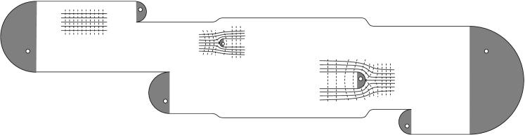
Figure 24: The quotient disk ${\mathcal{R}}$ and its foliation

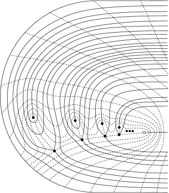
Figure 25: Detailed view of the shaded regions of Figure 24

The train track map $\phi\co\tau\includegraphics[height=7.22743pt]{backarr.eps}$ induces a map $\tilde{\Phi}\co{\mathcal{R}}\includegraphics[height=7.22743pt]{backarr.eps}$: unstable leaves (coming from horizontal segments) are stretched by the factor $\lambda$, stable leaves (coming from vertical segments) are contracted by the factor $1/\lambda$, the (projections of) rectangles are mapped as dictated by the action of $\phi$ on the real edges of $\tau$ and the identifications are mapped according to the action of $\phi$ on the infinitesimal edges of $\tau$.

7.2.2 Identifications of horizontal sides

The identifications of the horizontal sides of ${\mathcal{R}}$ are carried out in such a way as to restore the injectivity of $\tilde{\Phi}$ on $\partial{\mathcal{R}}$. In order to describe them, it is therefore necessary to understand the structure of $\partial{\mathcal{R}}$ and the action of $\tilde{\Phi}$ on it. This was the purpose of the analysis of the outside map of the unimodal map $f$ in Section 5: the dynamics of $\tilde{\Phi}|_{\partial{\mathcal{R}}}$ is modelled by the dynamics of the outside map, in a sense made precise by the following lemma.

Lemma 16.

Let $\theta\co S^{1}\to S^{1}\cup I$ be the outside map of $f$. Then there is a homeomorphism $h\co S^{1}\to\partial{\mathcal{R}}$ with the property that $\theta(x)\in S^{1}$ if and only if $\tilde{\Phi}(h(x))\in\partial{\mathcal{R}}$, and in this case $h(\theta(x))=\tilde{\Phi}(h(x))$.

Proof.

An analysis of the different possible configurations of infinitesimal edges in the junctions of $\mathbb{I}$, as given by Theorems 10 and 11, shows that for any kneading sequence $s\in\mathcal{M}\mathcal{I}\mathcal{A}$ the two corners on the left of $R_{1}$ are identified, the two corners on the right of $R_{N-1}$ are identified, and for $1\leq j<N-1$ the top (respectively bottom) right corner of $R_{j}$ is identified with the top (respectively bottom) left corner of $R_{j+1}$. The corners of the rectangles therefore define $2N-2$ points on $\partial{\mathcal{R}}$, which correspond naturally with the $2N-2$ points on $S^{1}$ defined by the critical orbit of $f$ (namely $\hat{a}$ and $\hat{b}$, together with $x_{l}$ and $x_{u}$ for each other point $x$ in the critical orbit).

Define $h\co S^{1}\to\partial{\mathcal{R}}$ to map each of these $2N-2$ points on $S^{1}$ to the corresponding point on $\partial{\mathcal{R}}$, and to map each interval of $S^{1}$ between two such points affinely onto the corresponding interval of $\partial{\mathcal{R}}$. Then $h$ is a homeomorphism, the points $x\in S^{1}$ with $\theta(x)\not\in S^{1}$ are precisely those for which $\tilde{\Phi}(h(x))\not\in\partial{\mathcal{R}}$, and away from these points both $\theta$ and $\tilde{\Phi}$ are affine on each of the $2N-2$ intervals, and send corresponding endpoints to corresponding endpoints. ∎

Abusing notation, let $\gamma\subseteq\partial{\mathcal{R}}$, $a,c,p\in\partial{\mathcal{R}}$ be defined as $h(\gamma)$, $h(\hat{a})$, $h(c_{u})$, $h(p_{u})$ respectively (see Figure 26).

\psfrag{eta0}{$\scriptstyle{\eta_{0}}$}\psfrag{eta-1}{$\scriptstyle{\eta_{-1}}$}\psfrag{eta-2}{$\scriptstyle{\eta_{-2}}$}\psfrag{gamma}{$\scriptstyle{\gamma}$}\psfrag{P(G)}[b]{$\scriptstyle{\tilde{\Phi}(\gamma)}$}\psfrag{P(c)}{$\scriptstyle{\tilde{\Phi}(c)}$}\psfrag{c}{$\scriptstyle{c}$}\psfrag{ha}{$\scriptstyle{a}$}\psfrag{p}{$\scriptstyle{p}$}\psfrag{q}[bl]{$\scriptstyle{q=\tilde{\Phi}(a)=\tilde{\Phi}(p)}$}\includegraphics[width=346.89731pt]{constr4}

Figure 26: ${\mathcal{R}}$ and its image under $\tilde{\Phi}$

Theorem 17.

Let $s=\kappa(F)$, and suppose that $q(s)=m/n\in(0,1/2)\cap\mathbb{Q}$. Then $\tilde{\Phi}|_{\partial{\mathcal{R}}}$ has a unique periodic orbit, which has period $n$ and rotation number $m/n$. The boundary ${\partial{\mathcal{R}}}$ has the structure of an $n$-sided polygon, with vertices the points $\tilde{\Phi}^{j}(a)$ for $1\leq j\leq n$. Moreover, $v=\tilde{\Phi}^{n}(a)\in\overline{\gamma}$ satisfies:

1. $v=a$ (so that $a$ is periodic under $\tilde{\Phi}$) if and only if $s=\operatorname{lhe}(m/n)$

2. $v=c$ if and only if $s=\operatorname{NBT}(m/n)$

3. $v=p$ (so that $p$ is periodic under $\tilde{\Phi}$) if and only if $s=\operatorname{rhe}(m/n)$

4. $v$ is strictly between $a$ and $c$ if and only if $\operatorname{lhe}(m/n)\prec s\prec\operatorname{NBT}(m/n)$

5. $v$ is strictly between $c$ and $p$ if and only if $\operatorname{NBT}(m/n)\prec s\prec\operatorname{rhe}(m/n)$

Proof.

The statements about the periodic orbit on ${\partial{\mathcal{R}}}$ and the position of $v$ are direct translations of Theorem 6. An analysis of the different possible configurations of infinitesimal edges in the junctions of $\mathbb{I}$ shows that there are singularities on ${\partial{\mathcal{R}}}$ corresponding to each junction with configuration $S^{\pm}$, and cusps on ${\partial{\mathcal{R}}}$ corresponding to each $2$-junction with configuration $BP$, $B$, $W^{\pm}$, $V_{1}^{\pm}B$, or $V_{2}^{\pm}B^{2}$. By Theorems 10 and 11, there are exactly $n$ such junctions, and these junctions are precisely those containing the first $n$ images under $F$ of the left hand $1$-junction. ∎

Remark 4.

Observe that if $s$ is not one of the endpoints of $\operatorname{KS}(m/n)$, then the vertices of ${\partial{\mathcal{R}}}$ correspond exactly to the vertices of the unbounded complementary component of $\tau$.

The m.u.s.c. decomposition giving the identifications on the horiztonal edges can now be described: as before, it is constructed using rectangular and semi-circular arc bands joining points on the horizontal edges which will be identified. These arc bands will be labelled $\eta_{j}$ for $j\leq 0$ (in fact $\eta_{j}$ will often denote a union of two arc bands), with the arcs of $\eta_{j}$ joining precisely those points of ${\partial{\mathcal{R}}}$ which are identified by $\tilde{\Phi}^{1-j}$ but not by $\tilde{\Phi}^{-j}$: thus $\tilde{\Phi}$ will project to a homeomorphism of the quotient space. In particular, $\eta_{0}$ is a semi-circular arc band centred at $c$ whose arcs join pairs of points of $\overline{\gamma}$ which are identified by $\tilde{\Phi}$. This is illustrated for the running example in Figure 26, where the image of $\gamma$ has been depicted slightly separated for clarity. Notice that $\tilde{\Phi}|_{{\partial{\mathcal{R}}}}^{-1}$ is discontinuous at $q=\tilde{\Phi}(a)=\tilde{\Phi}(p)$ and is not surjective since it misses $\gamma$, but away from $q$ it is a continuous injection (the injectivity is what makes it possible to construct the arc bands $\eta_{j}$ in such a way that they intersect ${\partial{\mathcal{R}}}$ with disjoint interiors).

The preimages $\gamma_{j}=\tilde{\Phi}^{j}(\gamma)$ are connected for $-n+1\leq j<0$, since $\overline{\gamma_{-n+1}}$ is the first preimage of $\overline{\gamma}$ which contains the point of discontinuity $q$ by Theorem 17. Thus the arc bands $\eta_{j}$ for $-n+1\leq j<0$ are semi-circular, centred on $c_{j}=\tilde{\Phi}^{j}(c)$, and can be chosen to be disjoint.

For $j\leq-n$ there are three different cases, according as $s$ is an endpoint of $\operatorname{KS}(m/n)$, is equal to $\operatorname{NBT}(m/n)$, or is neither. As in the statement of Theorem 17, let $v=\tilde{\Phi}^{n}(a)$ denote the vertex of ${\partial{\mathcal{R}}}$ which lies in $\overline{\gamma}$.

1. $s$ is an endpoint of $\operatorname{KS}(m/n)$: Then $v$ coincides with an endpoint of $\gamma$ and is periodic of period $n$. Thus $q$ is one of the endpoints of $\gamma_{-n+1}$ so the preimages $\gamma_{j}$ are connected for all $j<0$. The arc bands $\eta_{j}$ are semi-circular centred at $c_{j}$ for all $j\leq 0$. Since their sizes tend to $0$, they can be chosen to be disjoint away from their vertices and to have diameters tending to $0$ as $j\to-\infty$. They cover ${\partial{\mathcal{R}}}$ by Theorem 6, accumulate on the periodic orbit on ${\partial{\mathcal{R}}}$, and their vertices lie on the orbit of preimages of this periodic orbit (described in Theorem 6). Figure 27 depicts these arc bands in the case $s=\operatorname{lhe}(1/3)$: the white dots depict the points of the period $3$ orbit on ${\partial{\mathcal{R}}}$.

   \psfrag{0}{$\scriptstyle{\eta_{0}}$}\psfrag{-1}{$\scriptstyle{\eta_{-1}}$}\psfrag{-2}{$\scriptstyle{\eta_{-2}}$}\psfrag{-3}{$\scriptstyle{\eta_{-3}}$}\psfrag{-4}{$\scriptstyle{\eta_{-4}}$}\psfrag{-5}{$\scriptstyle{\eta_{-5}}$}\includegraphics[width=216.81pt]{constr5}

   Figure 27: The arc bands in case a): here $s=(101)^{\infty}=\operatorname{lhe}(1/3)$

   The m.u.s.c. decomposition consists of the following elements:

   1. the closure of the complement of ${\mathcal{R}}\cup\bigcup_{j=0}^{-\infty}\eta_{j}$, which is a closed topological disk bounded by infinitely many arcs, containing the periodic orbit on its boundary and the point at infinity in its interior;

   2. the arcs of each arc band $\eta_{j},j\leq 0$, except for those contained in elements of i);

   3. the points of $\operatorname{Int}({\mathcal{R}})$.

2. $s=\operatorname{NBT}(m/n)$: Then $v=c$, so $q=\tilde{\Phi}^{-n+1}(c)$ and the point of discontinuity of $\tilde{\Phi}|_{\partial{\mathcal{R}}}^{-1}$ coincides with the centre of $\eta_{-n+1}$. Thus $\overline{\gamma_{-n}}$ is the union of two arcs, and each point in each arc is paired with exactly one point in the other. Inductively, the same is true for $\overline{\gamma_{j}}$ for all $j\leq-n$: thus the $\eta_{j}$ for $j\leq-n$ can be chosen to be rectangular arc bands, one of whose boundaries coincides with the outer boundary of $\eta_{j+n}$ and the other with the inner boundary of $\eta_{j-n}$. The sizes of these arc bands decrease exponentially, and they cover ${\partial{\mathcal{R}}}$ by Theorem 6. They are depicted in Figure 28 for the case $s=\operatorname{NBT}(1/3)$. The m.u.s.c. decomposition consists of the following elements:

   \psfrag{c}{$\scriptstyle{c=v}$}\includegraphics[width=303.53267pt]{constr6}

   Figure 28: The arc bands in the NBT case: here $s=(10011)^{\infty}$

   1. the closure of the complement of ${\mathcal{R}}\cup\bigcup_{j=0}^{-\infty}\eta_{j}$, which is a closed topological disk bounded by $n$ arcs, having the points of the periodic orbit on ${\partial{\mathcal{R}}}$ for vertices, and containing the point at infinity in its interior;

   2. the arcs of each arc band $\eta_{j},j\leq 0$ (in this case, no such arc is contained in an element of i));

   3. the points of $\operatorname{Int}({\mathcal{R}})$.

3. $s$ is neither $\operatorname{NBT}(m/n)$ nor an endpoint of $\operatorname{KS}(m/n)$: As in case b), $\gamma_{j}$ has two connected components for $j\leq-n$. However, because $v\neq c$, one of the components of each such $\gamma_{j}$ is divided into two subarcs: the points of one subarc are paired with other points in the same subarc, while those in the other are paired with points in the other component of $\gamma_{j}$. In Figure 29, $\gamma_{-n+1}=\alpha_{1}\cup\alpha_{2}\cup\alpha_{3}$, points of $\tilde{\Phi}^{-1}(\alpha_{1})$ are paired to points of $\tilde{\Phi}^{-1}(\alpha_{3})$ whereas points of $\tilde{\Phi}^{-1}(\alpha_{2})$ are paired to points of $\tilde{\Phi}^{-1}(\alpha_{2})$ itself. Thus $\eta_{j}$ is the union of a semi-circular arc band and a rectangular arc band; the diameters of the semi-circular bands tend to $0$ as $j\to-\infty$, as do the sizes of the rectangular bands. The arc bands cover ${\partial{\mathcal{R}}}$ by Theorem 6.

   \psfrag{P}{$\scriptstyle{\tilde{\Phi}^{-1}}$}\psfrag{c}{$\scriptstyle{c}$}\psfrag{v}{$\scriptstyle{v}$}\psfrag{q}{$\scriptstyle{q}$}\psfrag{a}{$\scriptstyle{\alpha_{1}}$}\psfrag{b}{$\scriptstyle{\alpha_{2}}$}\psfrag{k}{$\scriptstyle{\alpha_{3}}$}\psfrag{d}{$\scriptstyle{\tilde{\Phi}^{-1}(\alpha_{1})}$}\psfrag{e}{$\scriptstyle{\tilde{\Phi}^{-1}(\alpha_{2})}$}\psfrag{f}{$\scriptstyle{\tilde{\Phi}^{-1}(\alpha_{3})}$}\psfrag{0}{$\scriptstyle{\eta_{0}}$}\psfrag{n}{$\scriptstyle{\eta_{-n}}$}\psfrag{c(n-1)}{$\scriptstyle{c_{n-1}}$}\includegraphics[width=346.89731pt]{constr7}

   Figure 29: The arc bands in case c)

   The m.u.s.c. decomposition consists of the following elements:

   1. the closures of the (infinitely many) complementary components of ${\mathcal{R}}\cup\bigcup_{j\leq 0}\eta_{j}$; there is one exterior $n$-gon containing $\infty$ and having the points in the periodic orbit on ${\partial{\mathcal{R}}}$ for vertices, and infinitely many 3-gons;

   2. the arcs of each arc band in $\eta_{j},j\leq 0$, except for those contained in elements of i);

   3. the points of $\operatorname{Int}({\mathcal{R}})$.

   The complete decomposition for the running example, which satisfies $\operatorname{lhe}(1/3)\prec s\prec\operatorname{NBT}(1/3)$, is shown in Figure 30.

   

   Figure 30: The complete second stage decomposition for the running example

Lemma 18.

Each of these decompositions is m.u.s.c. and none of its elements separates $\tilde{S}$.

Proof.

In case a), where the diameters of the arc bands tends to $0$, and case b), where the arc bands can be regarded as a finite number of semi-circular arc bands, the proof is straightforward. For case c), let $\zeta_{n}$ be a sequence of decomposition elements, and $x_{n}\to x$, $y_{n}\to y$ be convergent sequences with $x_{n},y_{n}\in\zeta_{n}$ for all $n$. Then it is required to show that $x$ and $y$ lie in the same decomposition element. As in the proof of Lemma 15, it can be assumed that either every $\zeta_{n}$ is an arc of a distinct rectangular arc band, or every $\zeta_{n}$ is a distinct complementary component. In both cases, both $x$ and $y$ lie on the boundary of the complementary component containing $\infty$. ∎

By Theorem 14 the quotient space is a topological sphere $S$, and by construction $\tilde{\Phi}$ projects to a homeomorphism $\Phi\co S\includegraphics[height=7.22743pt]{backarr.eps}$. The following theorem asserts that $\Phi$ is a generalized pseudo-Anosov map, and describes the orbits of 1-pronged singularities, which are the most important from the point of view of dynamics. Recall that an orbit $\{f^{n}(x)\,:\,n\in\mathbb{Z}\}$ of a homeomorphism $f\co X\includegraphics[height=7.22743pt]{backarr.eps}$ is homoclinic to a fixed point $p$ of $f$ if $f^{n}(x)\to p$ as $n\to\pm\infty$.

Theorem 19.

Let $s\in\mathcal{M}\mathcal{I}\mathcal{A}$ have height $q(s)=m/n\in(0,1/2)$ and let $\Phi_{s}\co S\includegraphics[height=7.22743pt]{backarr.eps}$ denote the associated homeomorphism constructed above. Then $\Phi_{s}$ is a generalized pseudo-Anosov map. Moreover, it has exactly one orbit of 1-pronged singularities which

1. is homoclinic to the point at infinity if and only if $s$ is an endpoint of the interval $\operatorname{KS}(m/n)$;

2. is finite if and only if $s=\operatorname{NBT}(m/n)$;

3. is backward asymptotic to the point at infinity and forward asymptotic to the periodic orbit determined by $s$ if and only if $\operatorname{lhe}(m/n)\prec s\prec\operatorname{NBT}(m/n)$ or $\operatorname{NBT}(m/n)\prec s\prec\operatorname{rhe}(m/n)$.

Proof.

Let $\pi\co S^{2}\to S$ denote the projection map given by the construction, and let $Q=\bigcup_{i=1}^{N-1}R_{i}$. Then $\pi(Q)=S$, since every fibre of $\pi$ intersects $Q$; and $\pi|_{\operatorname{Int}(Q)}$ is an embedding, since every fibre which intersects $\operatorname{Int}(Q)$ is trivial. Thus the foliations of $Q$ by horizontal and vertical line segments project to regular foliations of $\pi(\operatorname{Int}(Q))$, which are equipped with transverse measures induced by Euclidean distance in $Q$. The arc bands describe isometric identifications of segments of $\partial Q$, with vertical (respectively horizontal) segments always identified with other vertical (respectively horizontal) segments. Thus the measured foliations are also regular at points of $\pi(\partial Q)$ other than those which are the projections of vertices of arc bands, or centres of semi-circular arc bands. The foliations have a $1$-pronged singularity at $\pi(c)$ whenever $c$ is the centre of a semi-circular arc band. If $v$ is the vertex of an arc band, there are more possibilities.

1. If $v$ is the vertex of an arc band on the interior of a vertical segment of $\partial Q$ corresponding to a junction of any type other than $S^{\pm}$, then $\pi(v)$ is a $3$-pronged singularity.

2. If $v$ is the vertex of an arc band on a vertical segment of $\partial Q$ corresponding to a junction of type $S^{\pm}$, then $\pi(v)$ is an essential ($\infty$-pronged) singularity.

3. If $v$ is a vertex of an arc band on a horizontal segment in the case where $s$ is an endpoint of $\operatorname{KS}(m/n)$, then $\pi(v)$ is an essential singularity.

4. If $v$ is a vertex of an arc band on a horizontal segment in the case where $s=\operatorname{NBT}(m/n)$, then $\pi(v)$ is an $n$-pronged singularity if $v$ is a point of the periodic orbit on $\partial Q$, and is a regular point otherwise.

5. If $v$ is a vertex of an arc band on a horizontal segment in the case where $s\neq\operatorname{NBT}(m/n)$ and $s$ is not an endpoint of $\operatorname{KS}(m/n)$, then $\pi(v)$ is an essential singularity if $v$ is a point of the periodic orbit on $\partial Q$, and is a $3$-pronged singularity otherwise.

By considering the singularities corresponding to junctions of each given type, it can easily be seen that junctions of types $BP$, $B$, and $V_{0}$ give rise to only finitely many singularities, whereas all other types give rise to infinitely many singularities which accumulate on the periodic point in the associated junction. If $s\neq\operatorname{NBT}(m/n)$ then the singularities arising from arc bands on horizontal segments of $\partial Q$ accumulate on the point $\pi(P)$, where $P$ is the periodic orbit on $\partial Q$; while if $s=\operatorname{NBT}(m/n)$ then there are only finitely many such singularities.

Thus the singularities of the foliations of $S$ accumulate at only finitely many points. By construction, these foliations are invariant under $\Phi$, with the horizontal (unstable) foliation being expanded by a factor $\lambda>1$ and the vertical (stable) foliation being contracted by a factor $1/\lambda$. Hence $\Phi$ is a generalized pseudo-Anosov map as required.

To show that the one-pronged singularities arising from arc bands on the vertical sides of $\partial Q$ lie on a single orbit, it is necessary to consider the action of the train track map $\phi\co\tau\includegraphics[height=7.22743pt]{backarr.eps}$ on the bubbles of $\tau$. If $s=\operatorname{NBT}(m/n)$, then it is clear that the $n+2$ bubbles are permuted cyclically by $\phi$. In all other cases where $s$ is periodic, the proof of Theorem 10 shows that there is a bubble $B$ in junction $N$ which is the image of an infinitesimal edge in junction $\pi^{-1}(N)$ joining the two switches of the junction and passing above the puncture, and all other bubbles are images of this one. Hence the forwards $\Phi$-orbit of the $1$-pronged singularity corresponding to $B$ contains precisely all of the $1$-pronged singularities arising from arc bands on the vertical sides of $\partial Q$. Similarly, if $s$ is preperiodic then all of the bubbles of $\tau$ are images of the unique bubble $B$ of $\tau$ in junction $N$.

It is immediate from the construction of Section 7.2.2 that the one-pronged singularities arising from arc bands on the horizontal sides of $\partial Q$ are precisely the points of the backwards $\Phi$-orbit of the point $\pi(c)$, since the centres of the arc bands on ${\partial{\mathcal{R}}}$ are at the points $\tilde{\Phi}^{-j}(c)$ for $j\geq 0$. Since $\tilde{\Phi}(c)$ lies on the right hand edge of $Q$, it follows that $\Phi(\pi(c))$ is the unique one-pronged singularity corresponding to a bubble in junction $N$ whose preimage has not already been assigned, and hence the $1$-pronged singularities form a single orbit as required. That the asymptotics of this orbit are as given in the statement of the theorem follows directly from the facts about $1$-pronged singularities established earlier in the proof. ∎

Remark 5.

$s=10^{\infty}$ is the only element of $\mathcal{M}\mathcal{I}\mathcal{A}$ with height $0$, and was excluded from the construction above in order not to have to introduce exceptions into each statement about $\operatorname{KS}(m/n)$. It can, however, be treated in exactly the same way as other elements of $\mathcal{M}\mathcal{I}\mathcal{A}$: the invariant generalized train track, depicted in Figure 5, is described by

$$(S^{+}\,\,;\,\,B)$$

(and hence is unique among train tracks corresponding to strictly preperiodic kneading sequences in having a junction of type $S^{+}$), and the same construction can be applied starting with this train track to obtain a ‘tight horseshoe’. This has been described in [4].

8 The complex structure

In this section it is shown that the topological sphere $S$ constructed above carries a natural complex structure which makes it into a complex sphere. With respect to this structure the $\Phi$-invariant foliations become the horizontal and vertical trajectories of an integrable quadratic differential which is meromorphic away from finitely many essential singularities, with respect to which $\Phi$ is a Teichmüller mapping. This is a special case of results sketched in [4].

Theorem 20.

Let $s\in\mathcal{M}\mathcal{I}\mathcal{A}$, and let $\Phi_{s}\co S\includegraphics[height=7.22743pt]{backarr.eps}$ be the associated generalized pseudo-Anosov map. Then the Euclidean structure on the rectangles used in the construction of $S$ induces a complex structure on $S$, with respect to which it is a complex sphere.

Proof.

As in the proof of Theorem 19, let $\pi\co S^{2}\to S$ be the projection map given by the construction of $S$ and $Q=\bigcup_{i=1}^{N-1}R_{i}$, where the $R_{i}$ are the rectangles corresponding to the real edges of the invariant train track $\tau$. Since $\pi|_{\operatorname{Int}(Q)}$ is a homeomorphism onto its image, the Euclidean structure on $\operatorname{Int}(Q)$ induces a natural complex structure on $\pi(\operatorname{Int}(Q))$. Moreover, the conformal mappings $z\mapsto z^{2/k}$ (on the slit plane) induce complex structures on the neighbourhoods of each $k$-pronged singularity. Thus $S$ has a complex structure away from the finite set $\Sigma$ of accumulations of singularities of the invariant foliations. To establish the theorem, it is necessary to show that the complex structure on $S\setminus\Sigma$ regards each point of $\Sigma$ as a puncture rather than a hole. Using the theory of extremal length [1, 14], this can be accomplished by constructing a nested sequence of annuli converging to each point of $\Sigma$, the sum of whose moduli is divergent. The standard estimate

$$\operatorname{Mod}(A)\geq\frac{\operatorname{Width}(A)^{2}}{\operatorname{Area}(A)}$$

for the modulus of an annular region $A$ will be used, where $\operatorname{Width}(A)$ is the minimum distance between the two boundary components of $A$.

Let $q(s)=m/n$. If $s=\operatorname{NBT}(m/n)$ then $\Sigma$ is empty, and there is nothing to show. If $\operatorname{lhe}(m/n)\prec s\prec\operatorname{NBT}(m/n)$ or $\operatorname{NBT}(m/n)\prec s\prec\operatorname{rhe}(m/n)$ then there is one point of $\Sigma$ corresponding to each junction of type $W$, $V_{1}$, $V_{2}$, or $V_{3}$ (ie, each junction containing infinitely many infinitesimal edges), and one point of $\Sigma$ corresponding to the point at infinity. Finally, if $s=\operatorname{lhe}(m/n)$ or $s=\operatorname{rhe}(m/n)$ then $\Sigma$ contains a single point. This case is harder, since the annuli cannot be constructed locally in $Q$, and is treated first.

Case 1. $s=\operatorname{lhe}(m/n)$ or $s=\operatorname{rhe}(m/n)$

Suppose that $s=\operatorname{lhe}(m/n)$: the case $s=\operatorname{rhe}(m/n)$ is entirely analogous. Let $M$ be the transition matrix for the train track map $\phi\co\tau\includegraphics[height=7.22743pt]{backarr.eps}$, $\lambda$ be its Perron-Frobenius eigenvalue, and $y$ be its Perron-Frobenius eigenvector. A construction similar to that described below can be found in [9].

By Theorem 10, $\tau$ has $n-2$ infinitesimal edges which are not loops, one in each junction other than the leftmost and rightmost. Carrying out the identifications corresponding to these edges yields a Euclidean polygon $E$ with $n$ vertical and $n$ horizontal sides. Infinitely many other identifications are applied to produce $S$, each of which involves identifying the two halves of an identification interval on the boundary of $E$. The identification intervals on the vertical sides of $E$ are given by (the eigenvector entries corresponding to) the bubbles of $\tau$, while those on the horizontal sides are given by the map $\tilde{\Phi}$ and its backwards iterates, as described in the proof of Theorem 17.

The following notation will be used:

• $w_{v}$ is half the length of the longest identification interval on the vertical sides of $E$: in other words, $w_{v}$ is the largest entry of $y$ which corresponds to a bubble of $\tau$.

• $w_{h}$ is half the length of the longest identification interval on the horizontal sides of $E$ (this interval is denoted $\gamma$ in the proof of Theorem 17).

• $w=\min(w_{v},w_{h})$, $W=\max(w_{v},w_{h})$.

• $a^{0},a^{1},\ldots,a^{n-1}$ are the points of the periodic orbit on the boundary of $E$, labelled so that $a^{0}$ is the rightmost and $a^{i+1\bmod{n}}$ is the image of $a^{i}$. Thus $a^{1}$ is the leftmost point of the orbit, denoted $a$ in the proof of Theorem 17. Observe that each $a^{i}$ is a vertex of $E$.

• Each side of $E$ is the union of a sequence of adjacent identification intervals which converge to one of the points $a^{i}$. Denote by $(u^{i}_{j})_{j=0}^{\infty}$ (respectively $(v^{i}_{j})_{j=0}^{\infty}$) this sequence on the vertical (respectively horizontal) side of $E$ with endpoint $a^{i}$.

• $a^{i}_{j}$ and $a^{i}_{j+1}$ (respectively $b^{i}_{j}$ and $b^{i}_{j+1}$) are the endpoints of the identification interval $u^{i}_{j}$ (respectively $v^{i}_{j}$). Thus

  1. The vertical (respectively horizontal) side of $E$ containing the vertex $a^{i}$ has $a^{i}_{0}$ (respectively $b^{i}_{0}$) as its other vertex.

  2. $(a^{i}_{j})$ and $(b^{i}_{j})$ are both sequences converging to $a^{i}$. All of the points of $\bigcup_{i,j}\{a^{i}_{j},b^{i}_{j}\}\cup\bigcup_{i}\{a^{i}\}$ are identified to the point at infinity in $S$.

  3. $|u_{0}^{0}|=2w_{v}$ (where $|I|$ denotes the length of an interval $I$), and $|v_{0}^{i_{0}}|=2w_{h}$ for some $i_{0}$ (with the property that $a^{i_{0}}$ is the topmost point of the periodic orbit on the boundary of $E$).

  4. $$|u^{i}_{j}| = \frac{2w_{v}}{\lambda^{i+nj}}\qquad\text{ and}$$

     $$|v^{i}_{j}| = \frac{2w_{h}}{\lambda^{(i-i_{0}\bmod{n})+nj}}$$

     for $i=0,1,\ldots,n-1$ and $j\geq 0$.

• For each $j\geq 0$, let

  $$r_{j}=\frac{w}{\lambda^{(n-1)+nj}}.$$

  That is, $r_{j}$ is half the length of the smallest of the $2n$ identification intervals $u^{i}_{j}$ and $v^{i}_{j}$.

A sequence of nested annuli $X_{k}$, converging to the point at infinity, will now be constructed. Each $X_{k}$ will be given as the union of finitely many regions of three types.

Half-annuli

For $0\leq i<n$ and $1\leq j\leq k$, let $A^{i}_{j,k}$ (respectively $B^{i}_{j,k}$) be the half-annulus centred at $a_{j}^{i}$ (respectively $b_{j}^{i}$) with inner radius $r_{k+1}$ and outer radius $r_{k}$. (These are half-annuli bounded by Euclidean semicircles and segments of the boundary of $E$: see Figure 31.)

\psfrag{a1}{$\scriptstyle{a^{i}_{j-1}}$}\psfrag{a2}{$\scriptstyle{a^{i}_{j}}$}\psfrag{a3}{$\scriptstyle{a^{i}_{j+1}}$}\psfrag{A1}[l]{$\scriptstyle{A^{i}_{j-1,k}}$}\psfrag{A2}[l]{$\scriptstyle{A^{i}_{j,k}}$}\psfrag{A3}[l]{$\scriptstyle{A^{i}_{j+1,k}}$}\psfrag{u1}{$\scriptstyle{u^{i}_{j-1}}$}\psfrag{u2}{$\scriptstyle{u^{i}_{j}}$}\psfrag{rk}[l]{$\scriptstyle{r_{k}}$}\psfrag{rk+1}[l]{$\scriptstyle{r_{k+1}}$}\includegraphics[width=130.08731pt]{halfann}

Figure 31: The half-annuli $A^{i}_{j,k}$

The identification intervals which share $a^{i}_{j}$ as an endpoint are $u^{i}_{j-1}$ and $u^{i}_{j}$ and $r_{k}\leq|u^{i}_{j}|/2<|u^{i}_{j-1}|/2$, so $A^{i}_{j,k}$ meets the identification intervals $u^{i}_{j-1}$ and $u^{i}_{j}$ between $a^{i}_{j}$ and the centres of the intervals, as in Figure 31. The same argument applies to the half-annuli $B^{i}_{j,k}$.

After the identifications on the boundary of $E$ have been carried out, each $\bigcup_{j=1}^{k}A^{i}_{j,k}$ and each $\bigcup_{j=1}^{k}B^{i}_{j,k}$ is a strip of width $r_{k}-r_{k+1}$ and area $k\pi(r_{k}^{2}-r_{k+1}^{2})/2$.

Rectangular quarter-annuli

Figure 32 shows the half-annuli $A^{i}_{k,k}$ and $B^{i}_{k,k}$. The endpoints in $u_{k}^{i}$ of the boundary semicircles of $A^{i}_{k,k}$ lie in the half of $u_{k}^{i}$ which is further from $a^{i}$, and these endpoints are identified with two points in the half of $u_{k}^{i}$ nearer to $a^{i}$, which are denoted $z_{1}$ and $z_{2}$ in the figure. There are analogous points $z_{3}$ and $z_{4}$ identified with endpoints of the half-annulus $B^{i}_{k,k}$. Since the internal angle of $E$ at $a_{i}$ is $\pi/2$, it is possible to define a rectangular quarter-annulus $Z^{i}_{k}$ as shown in the figure, each of whose boundary components is the union of a horizontal and a vertical arc, joining either $z_{1}$ to $z_{3}$ or $z_{2}$ to $z_{4}$.

\psfrag{a1}[r]{$\scriptstyle{a^{i}_{k-1}}$}\psfrag{a2}[r]{$\scriptstyle{a^{i}_{k}}$}\psfrag{A1}[l]{$\scriptstyle{A^{i}_{k-1,k}}$}\psfrag{A2}[l]{$\scriptstyle{A^{i}_{k,k}}$}\psfrag{u1}[r]{$\scriptstyle{u^{i}_{k-1}}$}\psfrag{u2}[r]{$\scriptstyle{u^{i}_{k}}$}\psfrag{b1}{$\scriptstyle{b^{i}_{k-1}}$}\psfrag{b2}{$\scriptstyle{b^{i}_{k}}$}\psfrag{B1}[b]{$\scriptstyle{B^{i}_{k-1,k}}$}\psfrag{B2}[b]{$\scriptstyle{B^{i}_{k,k}}$}\psfrag{v1}[t]{$\scriptstyle{v^{i}_{k-1}}$}\psfrag{v2}[t]{$\scriptstyle{v^{i}_{k}}$}\psfrag{z1}[bl]{$\scriptstyle{z_{1}}$}\psfrag{z2}[bl]{$\scriptstyle{z_{2}}$}\psfrag{z3}[bl]{$\scriptstyle{z_{3}}$}\psfrag{z4}[bl]{$\scriptstyle{z_{4}}$}\psfrag{ai}{$\scriptstyle{a^{i}}$}\psfrag{Z}[bl]{$\scriptstyle{Z^{i}_{k}}$}\includegraphics[width=216.81pt]{Z}

Figure 32: The rectangular quarter-annulus $Z^{i}_{k}$

A rectangular quarter-annulus is used since the distance between $a^{i}$ and $z_{1}$ need not be equal to the distance between $a^{i}$ and $z_{3}$. The former distance is less than $\sum_{j=k}^{\infty}|u^{i}_{j}|$ and the latter is less than $\sum_{j=k}^{\infty}|v^{i}_{j}|$. Hence, for each $i$ and each $k$, the region

$$Y^{i}_{k}=Z^{i}_{k}\cup\bigcup_{j=1}^{k}A^{i}_{j,k}\cup\bigcup_{j=1}^{k}B^{i}_{j,k}$$

is (once the identifications have been carried out) a strip of width $r_{k}-r_{k+1}$ and area bounded above by

$$k\pi(r_{k}^{2}-r_{k+1}^{2})+(r_{k}-r_{k+1})\left(\sum_{j=k}^{\infty}|u^{i}_{j}|+\sum_{j=k}^{\infty}|v^{i}_{j}|\right).$$

Circular vertex annuli

The other vertices $a^{i}_{0}=b^{i^{\prime}}_{0}$ of $E$ have internal angle either $\pi/2$ or $3\pi/2$. At each such vertex, construct a (circular) quarter-annulus or three-quarter-annulus $D^{i}_{k}$ with radii $r_{k}$ and $r_{k+1}$, whose boundary components join points identified with endpoints of $A^{i}_{1,k}$ to points identified with endpoints of $B^{i^{\prime}}_{1,k}$. These partial annuli have areas bounded above by $\pi(r_{k}^{2}-r_{k+1}^{2})$.

After the identifications have been carried out,

$$X_{k}=\bigcup_{i=0}^{n-1}(Y^{i}_{k}\cup D^{i}_{k})$$

is an annulus of width $r_{k}-r_{k+1}$ and area bounded above by

$$n\left((k+1)\pi(r_{k}^{2}-r_{k+1}^{2})+(r_{k}-r_{k+1})\left(\sum_{j=k}^{\infty}|u^{i}_{j}|+\sum_{j=k}^{\infty}|v^{i}_{j}|\right)\right).$$

The annuli $X_{1}$ and $X_{2}$ in the case $s=\operatorname{lhe}(1/3)=(101)^{\infty}$ are depicted in Figure 33.

\psfrag{A212}[lb]{$\scriptstyle{A^{2}_{1,2}}$}\psfrag{A211}{$\scriptstyle{A^{2}_{1,1}}$}\psfrag{A222}{$\scriptstyle{A^{2}_{2,2}}$}\psfrag{D22}{$\scriptstyle{D^{2}_{2}}$}\psfrag{D21}{$\scriptstyle{D^{2}_{1}}$}\psfrag{Z22}{$\scriptstyle{Z_{2}^{2}}$}\psfrag{Z21}{$\scriptstyle{Z^{2}_{1}}$}\psfrag{B222}{$\scriptstyle{B^{2}_{2,2}}$}\psfrag{B212}{$\scriptstyle{B^{2}_{1,2}}$}\psfrag{B211}{$\scriptstyle{B^{2}_{1,1}}$}\psfrag{B111}[bl]{$\scriptstyle{B^{1}_{1,1}}$}\psfrag{D01}{$\scriptstyle{D^{0}_{1}}$}\psfrag{D02}{$\scriptstyle{D^{0}_{2}}$}\psfrag{a0}[bl]{$\scriptstyle{a_{0}}$}\psfrag{a1}{$\scriptstyle{a_{1}}$}\psfrag{a2}{$\scriptstyle{a_{2}}$}\psfrag{u00}[l]{$\scriptstyle{u^{0}_{0}}$}\psfrag{u01}[l]{$\scriptstyle{u^{0}_{1}}$}\psfrag{u10}[r]{$\scriptstyle{u^{1}_{0}}$}\psfrag{u11}[r]{$\scriptstyle{u^{1}_{1}}$}\psfrag{v00}[b]{$\scriptstyle{v^{0}_{0}}$}\psfrag{v01}[b]{$\scriptstyle{v^{0}_{1}}$}\psfrag{v20}{$\scriptstyle{v^{2}_{0}}$}\psfrag{v21}{$\scriptstyle{v^{2}_{1}}$}\includegraphics[width=407.60385pt]{101infty}

Figure 33: Annuli with divergent moduli sum surrounding the accumulation of singularities of $\Phi_{\operatorname{lhe}(1/3)}$

Now

$$r_{k}\pm r_{k+1}=\frac{w}{\lambda^{(n-1)+nk}}(1\pm\frac{1}{\lambda^{n}})$$

and

$$\sum_{j=k}^{\infty}|u^{i}_{j}|+\sum_{j=k}^{\infty}|v^{i}_{j}|\leq\sum_{j=k}^{\infty}\frac{4W}{\lambda^{nj}}=\frac{4W\lambda^{n}}{\lambda^{nk}(\lambda^{n}-1)},$$

so

$$\operatorname{Mod}(X_{k})\geq\frac{\operatorname{Width}(X_{k})^{2}}{\operatorname{Area}(X_{k})} \geq \frac{r_{k}-r_{k+1}}{n\left((k+1)\pi(r_{k}+r_{k+1})+\frac{4W\lambda^{n}}{\lambda^{kn}(\lambda^{n}-1)}\right)}$$

$$= \frac{C_{1}/\lambda^{nk}}{(C_{2}k+C_{3})/\lambda^{nk}}$$

$$= \frac{C_{1}}{C_{2}k+C_{3}},$$

where $C_{1}$, $C_{2}$, and $C_{3}$ depend only on $n$, $\lambda$, $w$, and $W$. Hence $\sum_{k\geq 1}\operatorname{Mod}(X_{k})$ diverges as required.

Case 2. $\operatorname{lhe}(m/n)\prec s\prec\operatorname{NBT}(m/n)$ or $\operatorname{NBT}(m/n)\prec s\prec\operatorname{rhe}(m/n)$

Consider first the accumulation of singularities in a junction of type $W^{\pm}$. In Figure 34 the identifications on $Q$ are indicated with dotted lines, and the shaded half-annuli $A_{k}$ project to nested annular regions in $S$ which converge to the accumulation of singularities $p$. If the width of the rectangle in which these half-annuli lie is less than half its height then not all of them can be constructed there: in this case, simply start with the first half-annulus $A_{k_{0}}$ which can be constructed.

\psfrag{c}{$\scriptstyle{c}$}\psfrag{A1}{$\scriptstyle{A_{0}}$}\psfrag{A2}{$\scriptstyle{A_{1}}$}\psfrag{A3}{$\scriptstyle{A_{2}}$}\includegraphics[width=216.81pt]{Wpunc}

Figure 34: Annuli with divergent moduli sum surrounding an accumulation of singularities of type $W$.

Let $\mu=\lambda^{-N}$, where $N$ is the period of $p$, let $w$ be the width of the annulus $A_{0}$, and denote by $c$ the size of the largest semi-circular arc band. Then $\operatorname{Width}(A_{k})=w\mu^{k}$, and the $k^{\rm th}$ semi-circular arc band has size $c\mu^{k}$.

The outer radius $R_{k}$ of $A_{k}$ is one half of the distance between the highest and lowest points of $A_{k}$, in other words

$$R_{k} = \frac{1}{2}\left(2w\sum_{j=k}^{\infty}\mu^{j}+2c\sum_{j=k}^{\infty}\mu^{j}\right)$$

$$= \frac{(w+c)\mu^{k}}{1-\mu}.$$

Thus

$$\operatorname{Area}(A_{k})=\frac{\pi}{2}\operatorname{Width}(A_{k})(2R_{k}-\operatorname{Width}(A_{k}))=C\mu^{2k},$$

where $C$ depends only on $\mu$, $w$, and $c$. Hence

$$\operatorname{Mod}(A_{k})\geq\frac{\operatorname{Width}(A_{k})^{2}}{\operatorname{Area}(A_{k})}=\frac{w}{C}$$

so that $\sum_{k\geq k_{0}}\operatorname{Mod}(A_{k})$ diverges as required.

Similar arguments apply to accumulations of singularities of types $V$. For a junction of type $V_{1}$, let $R$ and $R^{\prime}$ denote the adjacent rectangles, where $R$ is the rectangle adjacent to the switch to which all of the bubbles in the junction are attached. Then a sequence of half-annuli is constructed in $R$ as for junctions of type $W$, but rather than being completed to annuli by the identifications they are completed by corresponding half-annuli in $R^{\prime}$. The moduli of these annuli are again bounded below by a positive constant. Junctions of type $V_{2}$ are double covers of junctions of type $W$, and a sequence of annuli with moduli bounded below by a positive constant at an accumulation of type $W$ thus induces a similar sequence at an accumulation of type $V_{2}$. Accumulations of type $V_{3}^{\pm}$ (respectively $V_{1}B$, $V_{2}B^{2}$) are identical to those of type $W^{\pm}$ (respectively $V_{1}$, $V_{2}$) in a neighbourhood of the accumulation point.

Finally, consider the point at infinity. The pattern of identification of horizontal sides, described in Section 7.2.2, is an $n$-fold cover of the pattern in junctions of type $W$: there are $n$ points on the horizontal boundary of ${\mathcal{R}}$ which are identified to the point at infinity, and the identifications along the horizontal sides are given by an alternating sequence of rectangular and semi-circular arc bands whose sizes decay exponentially. ∎

References

[1]L V Ahlfors, Conformal invariants: topics in geometric function
theory, McGraw-Hill Series in Higher
Mathematics, McGraw-Hill Book Co. New York (1973) \MR0357743
[2]M Bestvina, M Handel, Train-tracks for surface
homeomorphisms, Topology 34 (1995) 109–140 \MR1308491
[4]A de Carvalho, Extensions, quotients and generalized
pseudo-Anosov maps, to appear in: “Graphs and patterns in mathematics and
theoretical physics (Stony Brook, NY, 2001)”, (AMS Proc. Sympos. Pure
Math.)
[5]A de Carvalho, T Hall, Pruning theory and Thurston’s
classification of surface homeomorphisms, J. Eur. Math. Soc. (JEMS) 3 (2001)
287–333 \MR1866160
[6]A de Carvalho, T Hall, Braid forcing and star-shaped
train tracks, Topology 43 (2004) 247–287 \MR2052964
[7]W de Melo, S van Strien,
One-dimensional dynamics, Springer Erbebnisse series (3) 25,
Springer-Verlag, Berlin (1993) \MR1239171
[8]R Devaney, An introduction to chaotic dynamical systems, second
edition, Addison-Wesley Publishing Company Advanced Book Program, Redwood
City, CA (1989) \MR1046376
[9]C Earle, F Gardiner,
Teichmüller disks and Veech’s -structures,
from: “Extremal Riemann surfaces (San Francisco, CA, 1995)”,
Contemp. Math. 201, Amer. Math. Soc. Providence, RI (1997) 165–189
\MR1429199
[10]J Franks, M Misiurewicz, Cycles for disk homeomorphisms
and thick trees, from: “Nielsen theory and dynamical systems (South Hadley,
MA, 1992)”, Contemp. Math. 152,
Amer. Math. Soc. Providence, RI (1993) 69–139 \MR1429199
[11]F R Gantmacher, The theory of matrices. Vols. 1, 2,
(translated by K A Hirsch), Chelsea
Publishing Co. New York (1959) \MR0107649
[12]T Hall, The creation of horseshoes, Nonlinearity 7 (1994)
861–924 \MR1275533
[13]A Katok, B Hasselblatt,
Introduction to the modern theory of dynamical systems,
Encyclopedia of Mathematics and its Applications 54, Cambridge
University Press, Cambridge (1995), with a supplementary chapter by
Katok and L Mendoza \MR1326374
[14]O Lehto, K I Virtanen,
Quasiconformal mappings in the plane, second edition,
(translated from the German by K W Lucas), Grundlehren series 126,
Springer-Verlag, New York (1973) \MR0344463
[15]J Milnor, W Thurston, On iterated maps of the
interval, from: “Dynamical systems (College Park, MD, 1986–87)”,
Springer Lecture Notes series 1342, Springer, Berlin (1988) 465–563
\MR0970571
[16]R Moore, Foundations of point set theory, AMS Colloquium
Publications XIII, Amer. Math.
Soc. Providence, RI (1962) \MR0150722
[17]W P Thurston, On the geometry and dynamics of diffeomorphisms
of surfaces, Bull. Amer. Math. Soc. 19 (1988) 417–431 \MR0956596