Asymptotic behaviour of watermelons

Abstract

A watermelon is a set of $p$ Bernoulli paths starting and ending at the same ordinate, that do not intersect. In this paper, we show the convergence in distribution of two sorts of watermelons (with or without wall condition) to processes which generalize the Brownian bridge and the Brownian excursion in $\mathbb{R}^{p}$. These limit processes are defined by stochastic differential equations. The distributions involved are those of eigenvalues of some Hermitian random matrices. We give also some properties of these limit processes.

1 Introduction

We call $(p,n)$-watermelon a set of $p$ Bernoulli paths of length $n$ that meet two conditions. The first condition concerns the starting points and the endpoints: the $i$-th path starts at level $2i-2$ and ends at level $k+2i-2$. The integer $k$ is called the deviation of the watermelon. The second condition is that the $p$ paths do not touch each other. An additional condition, called wall condition, can be imposed: the paths should not cross the $x$ axis. Watermelons constitute a particular configuration of vicious walkers describing the situation in which two or more walkers arriving in the same lattice site annihilate one another. This model was introduced by Fisher [8], who also gave a number of physical applications for watermelons.

We shall consider two sorts of $(p,2n)$-watermelons without deviation: watermelons with wall condition and watermelons without wall condition. They generalize the notion of Dyck path (or excursion) and Grand Dyck path (or bridge). These processes have many applications, for instance to random matrices and Young tableaux [1, 9, 15], to the study of graphs via bijections [3] and of course to physics [6, 8].

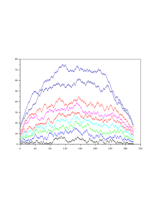
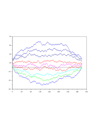
(a)	(b)

Figure 1: $(10,300)$-Watermelons with (a), and without (b) wall condition,

without deviation.

This paper contains three sections: the first section deals with watermelons with wall condition. We show that a $(p,2n)$-watermelon with wall condition, suitably rescaled in space (by $1/\sqrt{2n}$) and in time (by $1/(2n)$), converges in distribution to a stochastic process, that can be seen as the analog of a Brownian excursion for Dyson’s version of the $p$-dimensional Brownian motion [5]. This limit process is defined by a stochastic differential equation. It inherits the properties of watermelons with wall condition, namely its branches are positive (but at $0$ and $1$), and do not touch each other. For this reason we call the limit process continuous $p$-watermelon with wall condition. We also show, in agreement with [9], that the norm of such continuous $p$-watermelons is a Bessel bridge with dimension $p(2p+1)$.

In Section 2.2, we state similar results for watermelons without wall condition. The limit stochastic process is the $p$-dimensional analog of a Brownian bridge: the intrinsic Brownian bridge of the Weyl chamber $\{x\in\mathbb{R},x_{1}<\cdots<x_{p}\}$ (c.f. [4]). The norm of a continuous $p$-watermelon without wall condition is also a Bessel bridge, but, as expected, with dimension $p^{2}$. The proofs are given in Sections 3 and 4. They make essential use of a variant of Karlin Mac Gregor’ formulas ([11, 12, 14]) for the enumeration of non colliding paths: stars with fixed end points.

In the last Section, we give the expectation of the elementary symmetric polynomials of the positions of the continuous $p$-watermelon at time $t$, with or without wall condition. When $p=2$, we give the exact value of the moments of the two branches at time $t$.

In [13], Katori and Tanemura have shown that the vicious walkers with and without wall condition converge to the non-colliding Brownian motion (Dyson’s Brownian motion [5]) and the non-colliding Brownian meander. In these cases, the one-dimensional distribution of the limit processes are the eigenvalues of random matrices from a Gaussian Unitary Ensemble (GUE) and from a Gaussian Orthogonal Ensemble (GOE) ([15]). The watermelons that we study in this paper can be seen as vicious walkers constrained to return to $0$ at the end. Once rescaled, our one-dimensional distribusions are those of the eigenvalues of a Gaussian antisymmetric Hermitian matrices and a matrices from a GUE.

2 Main results

2.1 Watermelons with wall condition

Throughout the paper, $W^{(n)}_{i}(t)$ denotes the position at time $t\in[0,2n]$ of the $i$-th branch of a $(p,2n)$-watermelon with wall condition, and

$$X^{(n)}_{i}(t)=\frac{1}{\sqrt{2n}}W^{(n)}_{i}([2nt]).$$

We set

$$W^{(n)}(t)=(W^{(n)}_{i}(t))_{1\leq i\leq p}.$$

Thus

$$W^{(n)}=(W^{(n)}(t)),{t\in[0,2n]})$$

denotes a $(p,2n)$-watermelon with wall condition that starts and ends at $0$. We see it as a process in $\mathbb{R}^{p}$, more precisely in the Weyl chamber $\{x\in\mathbb{R}^{p},0<x_{1}<\cdots<x_{p}\}$. Similarly $X^{(n)}$ and $X^{(n)}(t)$ are related to a renormalized $(p,n)$-watermelon with wall condition.

We give a theorem about a stochastic differential equation (SDE) which allows us to define properly the limit process of $(p,2n)$-watermelons and we state a convergence theorem for watermelons. A few properties of this limit will be given in the sequel. These results are proved in section 3.

Let $H$ be a $(2p+1)\times(2p+1)$ Gaussian antisymmetric Hermitian matrix, and

$$\Lambda=(\lambda_{1},\dots,\lambda_{p})$$

the $p$ positive eigenvalues of $H$ sorted by increasing order. We know (cf. [15]) that the random variable $\Lambda$ has the density $f$ defined by

$$f(x)=c_{p}\prod_{1\leq i<j\leq p}({x_{j}}^{2}-{x_{i}}^{2})^{2}\,\prod_{i=1}^{p}x_{i}^{2}\ \mathrm{e}^{-\|x\|^{2}}1\mathrm{l}_{0\leq x_{1}\leq\cdots\leq x_{p}},$$

with

$$c_{p}=\frac{2^{3p/2}p!}{(2p)!\pi^{p/2}\displaystyle\prod_{1\leq i<j\leq p}(j-i)(j+i-1)}.$$

We have

Theorem 2.1.

The stochastic differential equation (SDE)

$$\left\{\begin{array}[]{l}\displaystyle\mathnormal{d}X_{i}(t)=\Big{(}\frac{-X_{i}(t)}{1-t}+\frac{1}{X_{i}(t)}+2X_{i}(t)\sum_{\begin{subarray}{c}j=1\\ j\neq i\end{subarray}}^{p}\frac{1}{X_{i}(t)^{2}-{X_{j}(t)^{2}}}\Big{)}\mathnormal{d}s+\mathnormal{d}B_{i}(t)\\ X_{i}(0)=0,\qquad\forall t\in\left]0;1\right[,\ X(t)\sim 2\sqrt{t(1-t)}\ \Lambda\end{array}\right. (E_{w})$$

has a unique strong solution $\big{(}(X_{i}(t))_{i=1\dots p},t\in\left[0,1\right]\big{)}$.

Theorem 2.2.

The process $X^{(n)}$ converges in distribution to the unique solution $X$ of the SDE $(E_{w})$.

This theorem will be proved in the section 3.3.

Remark 2.3.

The three terms of the drift coefficient in $(E_{w})$ reflect the different properties of the watermelons:

– the first term $-X_{i}(t)/(1-t)$ pushes the i-th path of $X$ to $0$ when $t$ is close to $1$.

– the second term $1/X_{i}(t)$ keeps the i-th path away from the x-axis.

– the third term $2X_{i}(t)/(X_{i}^{2}(t)-X_{j}^{2}(t))$ keeps the paths away from each other.

The first two terms are also present in the SDE for the normalized Brownian excursion,

$$\mathnormal{d}e(t)=\Big{(}\frac{-e(t)}{1-t}+\frac{1}{e(t)}\Big{)}\mathnormal{d}s+\mathnormal{d}B(t),$$

while the third is specific to watermelons.

Remark 2.4.

We shall see in section 3.1 (Proposition 3.1) that the Euclidean norm of the solution of $(E_{w})$ is a Bessel bridge ([16]) with dimension $p(2p+1)$.

Remark 2.5.

A solution of $(E_{w})$ has the same properties as a watermelon with wall condition: their paths do not touch each other, stay positive on $]0,1[$ (cf. Proposition 3.2) also they start and end at $0$. This is the reason why we call a solution of $(E_{w})$ continuous $p$-watermelon with wall condition.

2.2 Watermelons without wall condition

In this section, we consider $(p,2n)$-watermelon without wall condition. The results, and the proofs, given in section 4, are similar. Throughout the paper, we denote by

$$\widehat{W}^{(n)}=\big{(}(\widehat{W}_{i}^{(n)}(t))_{1\leq i\leq p},0\leq t\leq 2n\big{)}$$

a $(p,2n)$-watermelon without wall condition starting and ending at $0$ and

$$\big{(}\widehat{X}^{(n)}(t),t\in[0;1]\big{)}=\big{(}\frac{1}{\sqrt{2n}}\widehat{W}^{(n)}([2nt])),t\in[0;1]\big{)}$$

a renormalized $(p,2n)$-watermelon without wall condition.

Let $\widehat{H}$ be a matrix from a Gaussian Unitary Ensemble, we denote by

$$\widehat{\Lambda}=(\widehat{\lambda}_{1},\dots,\widehat{\lambda}_{p})$$

the $p$ eigenvalues of $\widehat{H}$ sorted in increasing order. We know (cf. [15]) that the random variable $\widehat{\Lambda}$ has the density $\widehat{f}$ defined by

$$\widehat{f}(x)=\frac{2^{-p/2}}{\pi^{p/2}\prod_{i=1}^{p-1}i!}\prod_{1\leq i<j\leq p}(x_{j}-x_{i})^{2}\ \mathrm{e}^{-\|x\|^{2}}1\mathrm{l}_{x_{1}\leq\cdots\leq x_{p}}.$$

We have

Theorem 2.6.

The stochastic differential equation

$$\left\{\begin{array}[]{l}\displaystyle\mathnormal{d}\widehat{X}_{i}(t)=\Big{(}\frac{-\widehat{X}_{i}(t)}{1-t}+\sum_{\begin{subarray}{c}j=1\\ j\neq i\end{subarray}}^{p}\frac{1}{\widehat{X}_{i}(t)-{\widehat{X}_{j}(t)}}\Big{)}\mathnormal{d}s+\mathnormal{d}B_{i}(t)\\ \widehat{X}(0)=0,\qquad\forall t\in]0;1[,\ \widehat{X}(t)\sim\sqrt{2t(1-t)}\ \widetilde{\Lambda}\end{array}\right. (E_{w/o})$$

has a unique strong solution $\widehat{X}=\big{(}(\widehat{X}_{i}(t))_{i=1\dots p},t\in\left[0,1\right]\big{)}$.

Theorem 2.7.

The process $\widehat{X}^{(n)}$ converges in distribution to the unique solution $\widehat{X}$ of $(E_{w/o})$.

Remark 2.8.

We shall see in section 4.1 (Proposition 4.1) that the Euclidean norm of the solution of $(E_{w/o})$ is a Bessel bridge with dimension $p^{2}$.

Remark 2.9.

A solution of $(E_{w/o})$ has the same properties as a watermelon without wall condition: their paths do not touch each other (cf. Proposition 4.2), start and end at $0$. This is the reason why we call a solution of $(E_{w/o})$ continuous $p$-watermelon without wall condition.

Remark 2.10.

In [4], Bougerol and Jeulin consider the Brownian bridge of length $T$ on a symmetric space of the non-compact type. They prove that this rescaled process converges when $T$ tends to infinity, to a limit process. The generalized radial part of this limit process is the bridge associated with the intrinsic Brownian motion in a Weyl chamber. For a suitable choice of the Weyl chamber, a watermelon without wall condition is the intrinsic Brownian bridge in this chamber. We thus have a geometric explanation of the dimension of the Bessel bridge corresponding to the Euclidean norm of the continuous $p$-watermelon.

3 Watermelons with wall condition: proofs

The existence of solutions of $(E_{w})$ is a consequence of the tightness of sequence $X^{(n)}$, and follows from the proof of Theorem 2.2. We focus first on uniqueness and properties of solutions of $(E_{w})$.

3.1 Properties

Proposition 3.1.

Let $X=(X_{1},\dots,X_{p})$ be a solution to the SDE $(E_{w})$. The Euclidean norm of $X$ is a Bessel bridge with dimension $p(2p+1)$.

Proof.

Set $V=\|X\|$. Applying Itô’s formula [16] to $V$, we obtain

$$\textnormal{d}V =\sum_{i=1}^{p}2X_{i}\textnormal{d}X_{i}+\sum_{i=1}^{p}\textnormal{d}<X_{i},X_{i}>$$

$$=\sum_{i=1}^{p}\Big{(}\frac{-2{X_{i}}^{2}}{1-t}+2+\sum_{j=1,j\neq i}^{p}\frac{4{X_{i}}^{2}}{{X_{i}}^{2}-{X_{j}}^{2}}\Big{)}\textnormal{d}t+\sum_{i=1}^{p}2X_{i}\textnormal{d}B_{i}+p\textnormal{d}t$$

$$=\Big{(}-\frac{2V}{1-t}+3p+\sum_{i,j=1,j\neq i}^{p}\frac{4{X_{i}}^{2}}{{X_{i}}^{2}-{X_{j}}^{2}}\Big{)}\textnormal{d}t+\sum_{i=1}^{p}2X_{i}\textnormal{d}B_{i}.$$

Now, we remark that

$$\sum_{i,j=1,j\neq i}^{p}\frac{4{X_{i}}^{2}}{{X_{i}}^{2}-{X_{j}}^{2}}=2p^{2}-2p$$

and that

$$\sum_{i=1}^{p}2X_{i}\textnormal{d}B_{i}=2\sqrt{V}\textnormal{d}\beta$$

where $\beta$ is a Brownian motion. We deduce from these equalities that $V$ is a solution of

$$\left\{\begin{array}[]{l}\textnormal{d}V=\Big{(}-\frac{2V}{1-t}+p(2p+1)\Big{)}\textnormal{d}t+2\sqrt{V}\textnormal{d}\beta,\\ V_{0}=0,\end{array}\right.$$

while we know that the squared Bessel bridge with dimension $p(2p+1)$ is another solution [16, Ch. XI]. ∎

Proposition 3.2.

If $X=(X_{1},\dots,X_{p})$ is a solution of $(E_{w})$, then

$$\mathbb{P}\left(\forall t\in\left]0;1\right[,\ 0<X_{1}(t)<\cdots<X_{p}(t)<+\infty\right)=1.$$

In other words, the paths of a solution of the equation $(E_{w})$ do not touch each other and stay positive on $\left]0;1\right[$.

Proof.

For every $\varepsilon\in\left]0;1/2\right[$, we prove the three relations:

$$\mathbb{P}\left(\forall t\in\left]\varepsilon;1-\varepsilon\right[,\ X_{p}(t)<+\infty\right)=1,$$ (5)

$$\mathbb{P}\left(\forall t\in\left]\varepsilon;1-\varepsilon\right[,\ X_{1}(t)<\cdots<X_{p}(t)\right)=1,$$ (6)

$$\mathbb{P}\left(\forall t\in\left]\varepsilon;1-\varepsilon\right[,\ X_{1}(t)>0\right)=1.$$ (7)

Relation (5) follows from Proposition 3.1: a Bessel bridge with dimension $p(2p+1)$ is almost surely finite.

Proof of relation (6). Let $(Z(t))_{\varepsilon\leq t\leq 1-\varepsilon}$ be defined by

$$Z(t)=\exp\left\{\sum_{i=1}^{p}\int_{\varepsilon}^{t}\frac{X_{i}(s)}{1-s}\textnormal{d}B_{i}(s)-\frac{1}{2}\int_{\varepsilon}^{t}\sum_{i=1}^{p}\left(\frac{X_{i}(s)}{1-s}\right)^{2}\textnormal{d}s\right\}$$

and define the probability measure $\mathbb{Q}$ by $\mathbb{Q}|_{\mathcal{F}_{t}}=Z(t)\mathbb{P}|_{\mathcal{F}_{t}}$, i.e.

$$\forall\Lambda\in\mathcal{F}_{t},\ \mathbb{Q}(\Lambda)=\mathbb{E}\left[Z(t)1{\rm l}_{\Lambda}\right].$$

According to the Girsanov Theorem [16], under $\mathbb{Q}$, $X$ is a solution of an homogeneous SDE:

$$\textnormal{d}X_{i}(t)=\Big{(}\frac{1}{X_{i}(t)}+\sum_{\begin{subarray}{c}j=1\\ j\neq i\end{subarray}}^{p}\frac{2X_{i}}{{X_{i}}^{2}-{X_{j}}^{2}}\Big{)}dt+\textnormal{d}\widetilde{B}(t),$$

in which $\widetilde{B}$ is a $\mathbb{Q}$-Brownian motion. Set

$$F(x_{1},\dots,x_{p})=\sum_{1\leq i<j\leq p}\ln\big{(}{x_{j}}^{2}-{x_{i}}^{2}\big{)},$$

and, for $t\in]\varepsilon,1-\varepsilon[$,

$$U(t)=F(X(t)).$$

Equivalently, relation (6) can be written

$$\mathbb{P}\left(\forall t\in\left]\varepsilon;1-\varepsilon\right[,\ U(t)>-\infty\right)=1.$$

Itô’s formula yields that:

$$\textnormal{d}U=\sum_{k=1}^{p}\Big{(}\frac{1}{X_{k}(t)}\frac{\partial F}{\partial x_{k}}+\big{(}\frac{\partial F}{\partial x_{k}}\big{)}^{2}+\frac{1}{2}\frac{\partial^{2}F}{{\partial x_{k}}^{2}}\Big{)}\textnormal{d}s+\sum_{k=1}^{p}\frac{\partial F}{\partial x_{k}}\textnormal{d}B_{k},$$ (8)

in which

$$\frac{\partial F}{\partial x_{k}}=\sum_{\begin{subarray}{c}j=1\\ j\neq k\end{subarray}}^{p}\frac{2x_{k}}{{x_{k}}^{2}-{x_{j}}^{2}},$$

and

$$\frac{\partial^{2}F}{{\partial x_{k}}^{2}}=\sum_{\begin{subarray}{c}j=1\\ j\neq k\end{subarray}}^{p}\Big{(}\frac{2}{{x_{k}}^{2}-{x_{j}}^{2}}-\frac{4{x_{k}}^{2}}{({x_{k}}^{2}-{x_{j}}^{2})^{2}}\Big{)}.$$

By symmetry,

$$\sum_{k=1}^{p}\sum_{\begin{subarray}{c}j=1\\ j\neq k\end{subarray}}^{p}\frac{1}{{x_{k}}^{2}-{x_{j}}^{2}}=0$$

and

$$\sum_{k=1}^{p}\sum_{\begin{subarray}{c}i,j=1\\ i\neq j\neq k\end{subarray}}^{p}\frac{{x_{k}}^{2}}{({x_{k}}^{2}-{x_{j}}^{2})({x_{k}}^{2}-{x_{i}}^{2})}=0,$$

where $i\neq j\neq k$ means $i\neq j$, $j\neq k$ and $i\neq k$. This leads to write (8) under the following form

$$\textnormal{d}U=S\textnormal{d}t+M\textnormal{d}\beta$$

in which $\beta$ is a $\mathbb{Q}$ Brownian motion,

$$S=2\sum_{\begin{subarray}{c}k,j=1\\ k\neq j\end{subarray}}^{p}\frac{{X_{k}}^{2}}{\big{(}{X_{k}}^{2}-{X_{j}}^{2}\big{)}^{2}},$$

and

$$M=\sqrt{\sum_{k=1}^{p}\Big{(}\frac{\partial F}{\partial x_{k}}\Big{)}^{2}}=\sqrt{2S}.$$

Let $\tau$ be the stopping time defined by

$$\tau =\inf\left\{\varepsilon\leq t\leq 1-\varepsilon,\ \exists\;i\in\left[{[}1,p\right]{]},\ X_{i}(t)=X_{i+1}(t)\right\}$$ (9)

$$=\inf\left\{\varepsilon\leq t\leq 1-\varepsilon,\ U(t)=-\infty\right\}$$

with the convention $\tau=1-\varepsilon$ if the infimum is not reach. We assume that $\mathbb{Q}(\tau<1-\varepsilon)>0$. As $S$ is positive, by standard comparison theorems (see for instance [10, p. 293]), there exists a solution $\widetilde{U}$ on $[\varepsilon;1-\varepsilon]$ of the SDE

$$\left\{\begin{array}[]{l}\textnormal{d}\widetilde{U}=M\textnormal{d}\beta\\ \widetilde{U}(\varepsilon)=U(\varepsilon).\end{array}\right.$$ (12)

such that

$$\forall t\in\left]\varepsilon,\tau\right[,\ \widetilde{U}(t)\leq U(t)\qquad\mathbb{Q}-a.s.$$

The previous inequality yields

$$\limsup_{t\to\tau}\widetilde{U}(t)\leq\lim_{t\to\tau}U(t)=-\infty\qquad\mathbb{Q}\text{-a.s.}$$

so that $\lim_{t\to\tau}\widetilde{U}(t)=-\infty$. By Dambis Dubins–Schwarz theorem [16, p.182], up to an enlargement of the filtered probability space, there exists a Brownian motion $\widetilde{\beta}$ such that for $t\in\left[\varepsilon;\tau\right[$,

$$\widetilde{U}(t)=\widetilde{U}(\varepsilon)+\widetilde{\beta}_{\int_{\varepsilon}^{t}M(s)\textnormal{d}s}.$$

Since $\widetilde{U}(t)$ has a limit when $t$ tends to $\tau$, it should be the same for the time-changed Brownian motion i.e.

$$0<\mathbb{Q}\big{(}\tau<1-\varepsilon\big{)}\leq\mathbb{Q}\big{(}\lim_{t\to\tau\wedge 1-\varepsilon}U(t)=-\infty\big{)}=\mathbb{Q}\big{(}\lim_{t\to\tau\wedge 1-\varepsilon}\widetilde{\beta}_{\int_{\varepsilon}^{t}M(s)}=\infty\big{)}.$$

This is absurd thus $\tau>1-\varepsilon$ $\mathbb{Q}$-a.s. Now $\{\tau>1-\varepsilon\}$ is $\mathcal{F}_{1-\varepsilon}$-measurable, hence

$$\mathbb{Q}(\{\tau>1-\varepsilon\})=\mathbb{E}\left[Z_{1-\varepsilon}1{\rm l}_{\tau>1-\varepsilon}\right]=1.$$

Since $\mathbb{E}\left[Z_{1-\varepsilon}\right]=1$, we have

$$\mathbb{P}\left(\{\tau\geq 1-\varepsilon\}\right)=1.$$

This evaluation proves the equality (6).

Proof of relation (7). Set

$$V=\ln(\prod_{i=1}^{p}X_{i})$$

and

$$A=\sum_{i=1}^{p}\frac{1}{{X_{i}}^{2}}.$$

By Itô’s formula, we obtain

$$\textnormal{d}V=\left[\frac{-p}{1-t}+\frac{A}{2}\right]\textnormal{d}t+\sqrt{A}\,\textnormal{d}\widetilde{B},$$

where $\widetilde{B}$ is a standard linear Brownian motion. Set

$$\widetilde{V}(t)=V(t)-V(\varepsilon)+\int_{\varepsilon}^{t}\left(\frac{p}{1-s}-\frac{A}{2}\right)\textnormal{d}s,$$ (13)

and

$$\sigma=\inf\big{\{}t\geq\varepsilon,\ X_{1}(t)=0\big{\}}.$$ (14)

Relation (13) has two consequences: $\widetilde{V}$ is a time-changed Brownian motion,

$$\widetilde{V}(t)=\widetilde{B}\Big{(}\int_{\varepsilon}^{t}\sqrt{A}\ \textnormal{d}s\Big{)},$$

and, if $\sigma\leq 1-\varepsilon$,

$$\lim_{t\to\sigma}\widetilde{V}(t)=-\infty.$$

Finally, this last event has null probability, by standard properties of Brownian paths, entailing $\mathbb{P}\left(\sigma\leq 1-\varepsilon\right)=0$. Relation (7) follows. ∎

Proof of Theorem 2.1.

We shall see in Section 3.3 that the existence of a solution of the SDE $(E_{w})$ is a consequence of the proof of Theorem 3.6. For $\varepsilon\in\left]0;1/2\right[$, we consider the SDE $(E_{\varepsilon})$ defined for $t\in\left[\varepsilon;1-\varepsilon\right]$ by

$$\left\{\begin{array}[]{l}\displaystyle\textnormal{d}X_{i}(t)=\Big{(}\frac{-X_{i}(t)}{1-t}+\frac{1}{X_{i}(t)}+2X_{i}(t)\sum_{\begin{subarray}{c}j=1\\ j\neq i\end{subarray}}^{p}\frac{1}{X_{i}(t)^{2}-{X_{j}(t)^{2}}}\Big{)}\textnormal{d}s+\textnormal{d}B^{i}_{t}\\ X_{i}(\varepsilon)\sim f(\varepsilon,x).\end{array}\right. E_{\varepsilon}$$ ()

It is clear that every solution of $(E_{w})$ is a solution of ($E_{\varepsilon}$). The coefficients of the SDE ($E_{\varepsilon}$) are locally Lipschitz in $\{0<x_{1}<\dots<x_{p}\}$ thus the strong uniqueness holds for the equation ($E_{\varepsilon}$) [10, p. 287] up to the explosion time of the solution i.e. on $\left[\varepsilon,\tau\wedge\sigma\right]$ where $\tau$ and $\sigma$ are defined by (9) and (14). By Proposition 3.2, $\tau\wedge\sigma$ is larger than $1-\varepsilon$, thus the strong uniqueness holds for the equation ($E_{\varepsilon}$) on $\left[\varepsilon,1-\varepsilon\right]$.

Let $X$ and $Y$ be two solutions of $(E_{w})$. For every $\varepsilon$ positive, $X$ and $Y$ are solutions of ($E_{\varepsilon}$). Using the uniqueness of ($E_{\varepsilon}$), we have

$$\forall\varepsilon>0,\qquad(X(t),\varepsilon\leq t\leq 1-\varepsilon)\overset{d}{=}(Y(t),\varepsilon\leq t\leq 1-\varepsilon).$$

Hence

$$(X(t),0<t<1)\overset{d}{=}(Y(t),0<t<1).$$

Finally, as $X(0)=Y(0)=X(1)=Y(1)=0$, the two processes $X$ and $Y$ have the same distribution. ∎

3.2 One-dimensional distribution

Now, we give a few results useful for the proof of Theorem 2.2. First, we prove that for a given $t$, the sequence $\big{(}X^{(n)}(t)\big{)}_{n\geq 1}$ converges in distribution to $X(t)$.

Proposition 3.3.

Let $X^{(n)}$ be a renormalized $(p,2n)$-watermelon with wall condition and let $t$ be in $[0;1]$. $X^{(n)}(t)$ converges in distribution to $2\sqrt{t(1-t)}\ \Lambda$.

Proof.

We denote by $f(t;x)$ the density function of $2\sqrt{t(1-t)}\ \Lambda$ i.e.

$$f(t;x)=\frac{c_{p}}{\big{(}t(1-t)\big{)}^{p^{2}+p/2}}\prod_{1\leq i<j\leq p}({x_{j}}^{2}-{x_{i}}^{2})^{2}\,\prod_{i=1}^{p}x_{i}^{2}\ \mathrm{e}^{-\frac{\|x\|^{2}}{2t(1-t)}}1\mathrm{l}_{0\leq x_{1}\leq\cdots\leq x_{p}},$$

and

$$c_{p}=\frac{2^{3p/2}p!}{(2p)!\pi^{p/2}\displaystyle\prod_{1\leq i<j\leq p}(j-i)(j+i-1)}.$$

For two vectors $u$ and $v$ in $\mathbb{R}^{p}$, $u\prec v$ means

$$\forall i\in\left[{[}1;p\right]{]},\qquad u_{i}<v_{i}.$$

Also, set

$$[u;v]=\{x\in\mathbb{R}^{p},\forall i\in\left[{[}1;p\right]{]},\ u_{i}<x_{i}<v_{i}\}$$

where $[{[}x;y]{]}$ is the set of integers in $[x;y]$. Let $u$ and $v$ be two vectors in $\mathbb{R}^{p}$ such that $0\prec u\prec v$ and let $t$ be in $\left[0;1\right]$. It suffices to prove that

$$\mathbb{P}\left(X^{(n)}(t)\in\left[u;v\right]\right)\underset{n\to\infty}{\longrightarrow}\int_{[u;v]}f(t;x)\mathnormal{d}x.$$

We have

$$\mathbb{P}\left(X^{(n)}(t)\in\left[u;v\right]\right)=\sum_{\begin{subarray}{c}u\leq x\leq v\\ x\sqrt{2n}\in\mathbb{N}\end{subarray}}\mathbb{P}\left(W^{(n)}([2nt])=x\sqrt{2n}\right).$$

Following [14], we call star a set of $p$ random walks, each of length $2n$, that satisfy the non-crossing condition and start at $0,2,\dots,2p-2$, respectively. The only difference between a star and a watermelon is that, in a star, the $y$-coordinates of the endpoints are unconstrained.

If we denote by $N(m,e)$ the number of stars of length $m$ with wall condition which end at $(e_{1},\dots,e_{2})$, we have (Theorem 6. of [14])

$$N(m,e)=2^{-p^{2}+p}\prod_{i=1}^{p}(e_{i}+1)\!\!\!\prod_{1\leq i<j\leq p}\!\!(e_{j}-e_{i})(e_{j}+e_{i}+2)\prod_{i=1}^{p}D(m,\frac{e_{i}}{\sqrt{2n}},p).$$ (17)

with

$$D(m,x_{i},p)=\frac{(m+2i-2)!}{(\mbox{\small$\frac{1}{2}$}(m+x_{i}\sqrt{2n})+p)!(\mbox{\small$\frac{1}{2}$}(m-x_{i}\sqrt{2n})+p-1)!}\cdot$$

Set $m=[2nt]$. A $(p,2n)$-watermelon which goes through $e$ at time $t$, can be cut in two stars: one of length $m$ and the other of length $2n-m$, both ending at $e$. The number of $(p,2n)$-watermelons is the number of stars of length $2n$ which end at $(0,2,\dots,2p-2)$. Regarding this, we have for $x$ such that $x\sqrt{2n}\in\mathbb{N}^{p}$

$$\mathbb{P}\left(W^{(n)}([2nt])=x\sqrt{2n}\right) =\frac{N(m,x\sqrt{2n})N(2n-m,x\sqrt{2n})}{N(2n,(2i-2)_{i})}$$

$$=c_{p,n}\prod_{i=1}^{p}\frac{D(m,x_{i},p)D(2n-m,x_{i},p)}{D(2n,\frac{2i-2}{\sqrt{2n}},+p)}$$

where

$$c_{p,n}=\frac{\displaystyle 2^{-p^{2}+p}\Big{[}\prod_{1\leq i<j\leq p}(x_{j}-x_{i})(x_{i}+x_{j}+\frac{2}{\sqrt{2n}})2n\Big{]}^{2}\Big{[}\prod_{i=1}^{p}(x_{i}+\frac{1}{\sqrt{2n}})\sqrt{2n}\Big{]}^{2}}{\displaystyle\prod_{1\leq i<j\leq p}4(j-i)(j+i-1)\prod_{i=1}^{p}(2i-1)}.$$

First we have the following estimate

$$c_{p,n}=\frac{2^{-p^{2}+3p}\ p!\ n^{p^{2}}}{(2p)!\displaystyle\prod_{1\leq i<j\leq p}(j-i)(j+i-1)}\prod_{1\leq i<j\leq p}\!\!\!({e_{j}}^{2}-{e_{i}}^{2})^{2}\prod_{i=1}^{p}{e_{i}}^{2}\Big{\{}1+\mathcal{O}\Big{(}\frac{1}{\sqrt{n}}\Big{)}\Big{\}}.$$

The lemma below gives an estimate of $D(m,e_{i},p)$.

Lemma 3.4.

Set $n,a,c,d\in\mathbb{N}$, $b\in\frac{1}{\sqrt{2n}}\mathbb{N}$ and $t\in\left]0;1\right]$. For $k=nt\{1+\mathcal{O}(\frac{1}{n})\}$, we have

$$\frac{(2k+a)!}{(k+b\sqrt{2n}+c)!(k-b\sqrt{2n}+d)!}=\frac{2^{2k+a}}{\sqrt{\pi}}(nt)^{a-c-d-\mbox{\small$\frac{1}{2}$}}\,\textnormal{e}^{-2{b}^{2}/t}\Big{\{}1+\mathcal{O}\Big{(}\frac{1}{\sqrt{n}}\Big{)}\Big{\}}$$

Furthermore, if $a$, $b$, $c$, $d$ and $t$ are in a compact set, then the $\mathcal{O}$ is uniform in all these variables.

Proof.

Using Stirling Formula and an asymptotic expansion of the logarithm, we obtain

$$(k+b\sqrt{2n}+c)!=\sqrt{2\pi k}\ k^{k+b\sqrt{2n}+c}\,\textnormal{e}^{-k+\frac{2b^{2}}{t}}\Big{\{}1+\mathcal{O}\Big{(}\frac{1}{\sqrt{n}}\Big{)}\Big{\}}.$$

We have in the same way

$$(k-b\sqrt{2n}+d)!=\sqrt{2\pi k}\ k^{k-b\sqrt{2n}+d}\,\textnormal{e}^{-k+\frac{2b^{2}}{t}}\Big{\{}1+\mathcal{O}\Big{(}\frac{1}{\sqrt{n}}\Big{)}\Big{\}}$$

and

$$(2k+a)!=\sqrt{4\pi k}\ (2k)^{2k+a}\,\textnormal{e}^{-2k}\Big{\{}1+\mathcal{O}\Big{(}\frac{1}{\sqrt{n}}\Big{)}\Big{\}},$$

leading to the result, after simplification. ∎

This lemma yields the following estimate of $D(m,x_{i},p)$:

$$D(m,x_{i},p)=\frac{1}{\sqrt{\pi}}(nt)^{2i-2p-\mbox{\small$\frac{3}{2}$}}2^{m+2i-2}\,\textnormal{e}^{-{x_{i}}^{2}/(2t)}\Big{\{}1+\mathcal{O}\Big{(}\frac{1}{\sqrt{n}}\Big{)}\Big{\}}$$

and so

$$\frac{D(m,x_{i},p)D(2n-m,x_{i},p)}{D(2n,\frac{2i-2}{\sqrt{2n}},p)}$$

$$=\frac{1}{\sqrt{\pi}}\big{(}nt(1-t) \big{)}^{2i-2p-\mbox{\small$\frac{3}{2}$}}2^{2i-2}\ \textnormal{e}^{-{x_{i}}^{2}/(2t(1-t))}\Big{\{}1+\mathcal{O}\Big{(}\frac{1}{\sqrt{n}}\Big{)}\Big{\}}.$$

We deduce that

$$\mathbb{P}\Big{(}W^{(n)}([2nt])= x\sqrt{2n}\Big{)}$$

$$=c_{p,n}\prod_{i=1}^{p}\frac{D(m,x_{i},p)D(2n-m,x_{i},p)}{D(2n,0,i-1+p)}$$

$$=c_{p}\frac{\prod_{1\leq i<j\leq p}({x_{j}}^{2}-{x_{i}}^{2})^{2}\prod_{i=1}^{p}{x_{i}}^{2}}{(2n)^{p/2}\big{(}t(1-t)\big{)}^{p^{2}+p/2}}\ \textnormal{e}^{-\frac{\|x\|^{2}}{2t(1-t)}}\Big{\{}1+\mathcal{O}\Big{(}\frac{1}{\sqrt{n}}\Big{)}\Big{\}}$$

$$=\Big{(}\frac{2}{n}\Big{)}^{p/2}f(t;x)\Big{\{}1+\mathcal{O}\Big{(}\frac{1}{\sqrt{n}}\Big{)}\Big{\}}$$

and finally

$$\mathbb{P}\left(X^{(n)}(t)\in\left[u,v\right]\right)=\Big{(}\frac{2}{n}\Big{)}^{p/2}\sum_{\begin{subarray}{c}u\leq x\leq v\\ e\sqrt{2n}\in\mathbb{N}\end{subarray}}f(t;x)\Big{\{}1+\mathcal{O}\Big{(}\frac{1}{\sqrt{n}}\Big{)}\Big{\}}.$$

In the equality above, the $\mathcal{O}$ is uniform in $x$ and can be factorized. Then, this expression becomes a Riemann sum which tends to $\int_{[u;v]}f(t;x)\textnormal{d}x$. Indeed, since the $x_{i}\sqrt{2n}$ have the same parity, the number of terms of a volume unit is $(\frac{\sqrt{2n}}{2})^{p}=(\frac{n}{2})^{p/2}$. ∎

3.3 Proof of Theorem 2.2

The following lemma explains that the probability that the branches of a $(p,2n)$-watermelon with and wall condition do not near $0$ or are relatively far from each other, tends to $1$ as $n$ tends to infinity. In the proof of Theorem 2.2, this lemma allows the restriction to such watermelons.

For $\varepsilon\in\left]0,1\right[$ and $\alpha\in\left]0,1/4\right[$, we define the sets

$$\Lambda_{n}^{1}(\alpha) =\left\{\exists k\in[{[}2\varepsilon n,((1-\varepsilon)\wedge\tau_{n}^{r})2n]{]},\ \exists i\in[{[}1,p]{]}\textnormal{ s.t. }W_{i}^{(n)}(k)\leq n^{\alpha}\right\}$$

$$=\left\{\exists k\in[{[}2\varepsilon n,((1-\varepsilon)\wedge\tau_{n}^{r})2n]{]},\textnormal{ s.t. }W_{1}^{(n)}(k)\leq n^{\alpha}\right\}$$

and

$$\Lambda_{n}^{2}(\alpha)=\left\{\exists k\in[{[}2\varepsilon n,((1-\varepsilon)\wedge\tau_{n}^{r})2n]{]},\ \exists i,j\in[{[}1,p]{]}\ \textnormal{ s.t. }i<j\text{ and}\right.\\ \hskip 170.71652pt\left.W_{j}^{(n)}(k)^{2}-W_{i}^{(n)}(k)^{2}\leq n^{\alpha}\right\}$$

where $r>0$ and $\tau_{n}^{r}=\inf\{t>\varepsilon,\ X^{(n)}_{p}(t)\leq r\}$ . We have

Lemma 3.5.

For $i\in\{1,2\}$,

$$\lim_{n\to\infty}\mathbb{P}\left(\Lambda_{n}^{i}(\alpha)\right)=0.$$

Proof.

We have shown in Proposition 3.3 that

$$\mathbb{P}\left(X^{(n)}(t)\in\left[u;v\right]\right)=\frac{1}{(2n)^{p/2}}\sum_{\begin{subarray}{c}u\sqrt{2n}\leq x\sqrt{2n}\leq v\sqrt{2n}\\ x\sqrt{2n}\in\mathbb{N}\end{subarray}}f(t;x)\Big{\{}1+\mathcal{O}\Big{(}\frac{1}{\sqrt{n}}\Big{)}\Big{\}}.$$

Thus for $t\in\left[\varepsilon,(1-\varepsilon)\right]$, we have

$$\mathbb{P}\Big{(}W_{1}^{(n)}([2nt])\in\left[0,n^{\alpha}\right] ,\ t\leq\tau_{n}^{r}\Big{)}$$

$$\leq\mathbb{P}\left(X^{(n)}(t)\in\left[0,n^{\alpha-1/2}\right]\times\left[0,r\right]^{p-1}\right)$$

$$=\frac{1}{(2n)^{p/2}}\sum_{\begin{subarray}{c}0\leq x_{1}\leq n^{\alpha-1/2}\\ x_{1}\sqrt{2n}\in\mathbb{N}\end{subarray}}\sum_{\begin{subarray}{c}0\leq x_{i}\leq r\\ x_{i}\sqrt{2n}\in\mathbb{N}\\ i=2\dots p\end{subarray}}f(t;x)\Big{\{}1+\mathcal{O}\Big{(}\frac{1}{\sqrt{n}}\Big{)}\Big{\}}.$$

Since $t\in[\varepsilon,(1-\varepsilon)]$ and $x_{1}\leq n^{\alpha-1/2}$,

$$f(t;x) \leq c_{p}\frac{\prod_{1\leq i<j\leq p}({x_{j}}^{2}-{x_{i}}^{2})^{2}\prod_{i=1}^{p}{x_{i}}^{2}}{\big{(}\varepsilon(1-\varepsilon)\big{)}^{p^{2}+p/2}}\ \textnormal{e}^{-2({x_{2}}^{2}+\cdots+{x_{p}}^{2})}$$

$$\leq\sum_{k=2}^{4p-2}{x_{1}}^{k}f_{k}(x_{2},\dots,x_{p})\leq\sum_{k=2}^{4p-2}{x_{1}}^{2}f_{k}(x_{2},\dots,x_{p})$$

$$\leq n^{2\alpha-1}\sum_{k=2}^{4p-2}f_{k}$$

where $f_{k}$ is the product of a polynomial with positive coefficients and of an exponential term $\exp(-2({x_{2}}^{2}+\cdots+{x_{p}}^{2}))$, in particular $f_{k}$ is integrable. Using the previous majoration, we obtain

$$\mathbb{P}\left(W_{1}^{(n)}([2nt])\in\left[0,n^{\alpha}\right],\ t\leq\tau_{n}^{r}\right)\\ \leq\frac{1}{\sqrt{2n}}\sum_{\begin{subarray}{c}0\leq x_{1}\leq n^{\alpha-1/2}\\ x_{1}\sqrt{2n}\in\mathbb{N}\end{subarray}}\frac{1}{(2n)^{(p-1)/2}}\sum_{\begin{subarray}{c}0\leq x_{i}\leq r\\ x_{i}\sqrt{2n}\in\mathbb{N}\\ i=2\dots p\end{subarray}}n^{2\alpha-1}\sum_{k=2}^{4p-2}f_{k}\Big{\{}1+\mathcal{O}\Big{(}\frac{1}{\sqrt{n}}\Big{)}\Big{\}}.$$

The sum over the $x_{i}$ for $i\in\{2,\dots,p\}$ is a Riemann sum, thus

$$\frac{1}{(2n)^{(p-1)/2}}\sum_{\begin{subarray}{c}0\leq x_{i}\leq r\\ x_{i}\sqrt{2n}\in\mathbb{N}\\ i=2\dots p\end{subarray}}\sum_{k=2}^{4p-2}f_{k}=\int_{0}^{r}\sum_{k=2}^{4p-2}f_{k}(x)\textnormal{d}x\ \left\{1+\mathcal{O}\left(\frac{1}{n}\right)\right\}\leq c$$

where $c$ is a positive constant, leading to:

$$\mathbb{P}\left(W_{1}^{(n)}([2nt])\in\left[0,n^{\alpha}\right],\ t\leq\tau_{n}^{r}\right)\leq cn^{3(\alpha-1/2)}.$$

Finally, for $\alpha\leq 1/4$,

$$\mathbb{P}\left(\Lambda_{n}^{1}(\alpha)\right) \leq\mathbb{P}\left(\exists k\leq 2\big{(}(1-\varepsilon)\wedge\tau_{n}^{r}-\varepsilon\big{)}n^{1-\alpha},\ W_{1}^{(n)}(2\varepsilon n+kn^{\alpha})\leq 2n^{\alpha}\right)$$

$$\leq\sum_{k=0}^{(1-2\varepsilon)2n^{1-\alpha}}\mathbb{P}\left(W_{1}^{(n)}(2\varepsilon n+kn^{\alpha})\leq 2n^{\alpha},\ \varepsilon+\frac{kn^{\alpha}}{2n}\leq\tau_{n}^{r}\right)$$

$$\leq 2cn^{3(\alpha-1/2)}(1-2\varepsilon)n^{1-\alpha}$$

$$\leq 2cn^{2\alpha-1/2}.$$

entailing the first point.

For $i=2$, we proceed as above. Set

$$\Lambda_{n}^{2}(\alpha)=\bigcup_{j=1}^{p-1}\Lambda_{n}^{2,j},$$

in which

$$\Lambda_{n}^{2,j}=\left\{\exists k\in[{[}2\varepsilon n,((1-\varepsilon)\wedge\tau_{n}^{r})2n]{]},\text{ s.t. }W_{j+1}^{(n)}(k)^{2}-W_{j}^{(n)}(k)^{2}\leq n^{\alpha}\right\}.$$

Let us fix $j\in[1,p-1]$. For $t\in[\varepsilon,(1-\varepsilon)]$, Proposition 3.3 yields

$$\mathbb{P}\left(W_{j+1}([2nt])^{2}-W_{j}([2nt])^{2}\in[0,n^{\alpha}],\ t\leq\tau_{n}^{r}\right)\\ =\frac{1}{(2n)^{p/2}}\sum_{\begin{subarray}{c}0\leq x_{i}\leq r,\ x_{i}\sqrt{2n}\in\mathbb{N}\\ {x_{j+1}}^{2}-{x_{j}}^{2}\leq n^{\alpha-1}/2\end{subarray}}f(t;x)\Big{\{}1+\mathcal{O}\Big{(}\frac{1}{\sqrt{n}}\Big{)}\Big{\}}.$$

replacing ${x_{j+1}}^{2}$ with $({x_{j+1}}^{2}-{x_{j}}^{2})+{x_{j}}^{2}$ in $f(t;x)$, we bound this function when $t\in[\varepsilon,1-\varepsilon]$ and ${x_{j+1}}^{2}-{x_{j}}^{2}\leq n^{\alpha-1/2}$:

$$f(t;x) \leq c_{p}\frac{\prod_{1\leq i<j\leq p}({x_{j}}^{2}-{x_{i}}^{2})^{2}\prod_{i=1}^{p}{x_{i}}^{2}}{\big{(}\varepsilon(1-\varepsilon)\big{)}^{p^{2}+p/2}}\ \textnormal{e}^{-2({x_{1}}^{2}+\cdots+{x_{p}}^{2})}$$

$$\leq\sum_{k=2}^{4p-2}\Big{(}{x_{j+1}}^{2}-{x_{j}}^{2}\Big{)}^{k}f_{k}(x_{1},\dots,x_{j},x_{j+2},\dots,x_{p})\leq n^{2\alpha-1}\sum_{k=2}^{4p-2}f_{k}$$

where the $f_{k}$ are products of an exponential term $\exp\big{(}-2({x_{1}}^{2}+\dots+{x_{j}}^{2}+{x_{j+2}}^{2}+\dots+{x_{p}}^{2})\big{)}$ with polynomials. Set $y={x_{j+1}}^{2}-{x_{j}}^{2}$, we have

$$\mathbb{P}\left(W_{1}^{(n)}([2nt])\in\left[0,n^{\alpha}\right],\ t\leq\tau_{n}^{r}\right)$$

$$\leq\frac{1}{\sqrt{2n}}\sum_{\begin{subarray}{c}0\leq x_{j}\leq r\\ x_{j}\sqrt{2n}\in\mathbb{N}\end{subarray}}\sum_{\begin{subarray}{c}0\leq y\leq n^{\alpha-1}\\ 2ny\in\mathbb{N}\end{subarray}}\frac{1}{(2n)^{(p-1)/2}}\sum_{\begin{subarray}{c}0\leq x_{i}\leq r\\ x_{i}\sqrt{2n}\in\mathbb{N}\\ i\neq j,j+1\end{subarray}}n^{2\alpha-1}\sum_{k=2}^{4p-2}f_{k}\Big{\{}1+\mathcal{O}\Big{(}\frac{1}{\sqrt{n}}\Big{)}\Big{\}}$$

$$\leq n^{3(\alpha-1/2)}\frac{1}{(2n)^{(p-1)/2}}\sum_{\begin{subarray}{c}0\leq x_{i}\leq r\\ x_{i}\sqrt{2n}\in\mathbb{N}\\ i\neq j+1\end{subarray}}\sum_{k=2}^{4p-2}f_{k}\Big{\{}1+\mathcal{O}\Big{(}\frac{1}{\sqrt{n}}\Big{)}\Big{\}}.$$

Now the $\mathcal{O}$ are uniform and the sum over the $x_{i}$ is a Riemann sum thus

$$\frac{1}{(2n)^{(p-1)/2}}\sum_{\begin{subarray}{c}0\leq x_{i}\leq r\\ xi\sqrt{2n}\in\mathbb{N}\\ i\neq j+1\end{subarray}}\sum_{k=2}^{4p-2}f_{k}=\int_{[0;r]^{p}}\sum_{k=2}^{4p-2}f_{k}(x)\textnormal{d}x\ \left\{1+\mathcal{O}\left(\frac{1}{n}\right)\right\}\leq c$$

where $c$ is a positive constant. This provides the following upper bound

$$\mathbb{P}\left(W_{j+1}^{(n)}([2nt])^{2}-W_{j}^{(n)}([2nt])^{2}\in\left[0,n^{\alpha}\right],\ t\leq\tau_{n}^{r}\right)\leq cn^{3(\alpha-1/2)}.$$

To complete this proof, notice that we have

$$\mathbb{P}\Big{(} \Lambda_{n}^{2,i}(\alpha)\Big{)}$$

$$\leq\mathbb{P}\left(\exists k\leq 2\big{(}(1-\varepsilon)\wedge\tau_{n}^{r}-\varepsilon\big{)}n^{1-\alpha},\ W_{j+1}^{(n)}(t_{k})^{2}-W_{j}^{(n)}(t_{k})^{2}\leq 3n^{\alpha}\right)$$

$$\leq\sum_{k=0}^{(1-2\varepsilon)n^{1-\alpha}}\mathbb{P}\left(W_{j+1}^{(n)}(t_{k})^{2}-W_{j}^{(n)}(t_{k})^{2}\leq 3n^{\alpha},t_{k}\leq\tau_{n}^{r}\right)$$

$$\leq c^{\prime}n^{3(\alpha-1/2)}(1-2\varepsilon)n^{1-\alpha}\leq c^{\prime\prime}n^{2\alpha-1/2}$$

where $t_{k}=2\varepsilon n+kn^{\alpha}$, $c^{\prime}$ and $c^{\prime\prime}$ are constants and that $\alpha$ is less than $1/4$.

∎

Proof of Theorem 2.2.

Let

$$\widetilde{X}^{(n)}=(\widetilde{X}^{(n)}(t),t\in[0;1])$$

be the piecewise constant process in $\mathbb{R}^{p}$ such that for every $k\in[{[}0,2n]{]}$ and every $i\in[{[}1,p]{]}$,

$$\widetilde{X}^{(n)}_{i}(\frac{k}{2n})=\frac{1}{\sqrt{2n}}(W_{i}^{(n)}(k)+1).$$

We consider here sample paths that belong to the space $\mathcal{D}$ of cad-lag (right continuous left limit) functions endowed with the Skorokhod topology (cf. [2, ch 2]). To prove this theorem, it suffices to show that the process $(\widetilde{X}^{(n)}(t))_{t}$ converges in distribution to the process $X$. The convergence in distribution of the process will be a consequence of Theorem 3.6 below. $(\widetilde{X}^{(n)}(t),t\in[\varepsilon,1-\varepsilon])$ to the process $(X(t),t\in[\varepsilon,1-\varepsilon])$ for every $\varepsilon\in]0;1/2[$. First, let us show that this convergence entails Theorem 2.2. Then we shall state and prove Theorem 3.6. Finally we shall apply this theorem to our case.

If we prove that $\widetilde{X}^{(n)}$ converges to $X$ on $[\varepsilon;1-\varepsilon]$ for every $\varepsilon\in]0;1/2[$, then the uniqueness of the solution of $(E_{w})$ implies that $(\widetilde{X}^{(n)}(t),t\in]0;1[)$ converges to $(X(t),t\in]0;1[)$. Since $X$ tends to $0$ when $t$ tends to $0$ and $1$, we have the convergence on $[0;1]$.

Theorem 3.6 is similar to Theorem 4.1 in [7].

Theorem 3.6.

We assume the strong uniqueness of the solution of the SDE

$$\mathnormal{d}X(t)=b(X(t),t)\mathnormal{d}t+\sigma(X(t),t)\mathnormal{d}B(t).$$ (18)

which satisfies a property $\mathcal{P}$. Let $X^{(n)}$ and $B^{(n)}$ be two processes with cad-lag sample paths on $\left[0,1\right]$ and let $A^{(n)}=(A_{i,j}^{(n)})$ be a symmetric $d\times d$ matrix-valued process such that $A_{i,j}^{(n)}$ has cad-lag sample paths on $\left[0,1\right]$ and $A^{(n)}(t)-A^{(n)}(s)$ is nonnegative definite for $t>s\geq 0$. Set

$$\tau_{n}^{r}=\inf\{t>0\text{ such that }|X^{(n)}(t)|\geq r\ or\ |X^{(n)}(t^{-})|\geq r\}$$

and $\mathcal{F}^{n}_{t}=\sigma(X^{(n)}(s),B^{(n)}(s),A^{(n)}(s),s\leq t)$.

We assume that the following assumptions hold for every $r>0$, $T>0$ and $i,j=1,\dots,d$:

$$M^{(n)}_{i}=X_{i}^{(n)}-B_{i}^{(n)}\text{ is a $\mathcal{F}_{t}^{n}$-local martingale }$$ (H1)

$$M_{i}^{(n)}M_{j}^{(n)}-A_{ij}^{(n)}\text{ is a $\mathcal{F}_{t}^{n}$-local martingale}$$ (H2)

$$\lim_{n\to\infty}\mathbb{E}\bigg{[}\sup_{t\leq T\wedge\tau_{n}^{r}}\big{|}X^{(n)}(t)-X^{(n)}(t^{-})\big{|}^{2}\bigg{]}=0$$ (H3)

$$\lim_{n\to\infty}\mathbb{E}\bigg{[}\sup_{t\leq T\wedge\tau_{n}^{r}}\big{|}B^{(n)}(t)-B^{(n)}(t^{-})\big{|}^{2}\bigg{]}=0$$ (H4)

$$\lim_{n\to\infty}\mathbb{E}\bigg{[}\sup_{t\leq T\wedge\tau_{n}^{r}}\big{|}A_{ij}^{(n)}(t)-A_{ij}^{(n)}(t^{-})\big{|}^{2}\bigg{]}=0$$ (H5)

$$\sup_{t\leq T\wedge\tau_{n}^{r}}\bigg{|}B_{i}^{(n)}(t)-\int_{0}^{t}b_{i}(X^{(n)}(s),s)\mathnormal{d}s\bigg{|}\overset{\mathbb{P}}{\longrightarrow}0$$ (H6)

$$\sup_{t\leq T\wedge\tau_{n}^{r}}\bigg{|}A_{ij}^{(n)}(t)-\int_{0}^{t}a_{ij}(X^{(n)}(s),s)\mathnormal{d}s\bigg{|}\overset{\mathbb{P}}{\longrightarrow}0$$ (H7)

where $(a_{ij})=\sigma\sigma^{*}$. Moreover, we assume that every accumulation point of $X^{(n)}$ satisfies the property $\mathcal{P}$ and that $X^{(n)}(0)$ converges in distribution to $X(0)$.

Then the process $(X^{(n)})_{n}$ converges in distribution to the process $X$.

Proof.

We shall prove this theorem in two steps whether the coefficients are homogeneous in time or not.

– Let us assume that the coefficients $\sigma$ and $b$ are homogeneous in time.

Using the same arguments as in the proof of Theorem 4.1 in [7], the sequence $\big{(}X^{(n)}(.\wedge\tau_{n}^{r})\big{)}$ is relatively compact and a limit $X^{r_{0}}$ of a subsequence of $\big{(}X^{(n)}(.\wedge\tau_{n}^{r_{0}})\big{)}$ is a solution of (18).

As $X^{r_{0}}$ is an accumulation point of the sequence $X^{(n)}$, the property $\mathcal{P}$ holds for $X^{r_{0}}$, thus, by uniqueness, $X^{r_{0}}$ has the same distribution as $X$. Therefore $X^{(n)}(.\wedge\tau_{n}^{r})$ converges in distribution to $X(.\wedge\tau^{r})$ for every $r>0$. But $\tau^{r}$ tends to infinity along with $r$. Thus $X^{(n)}$ converges in distribution to $X$.

– When the coefficients $\sigma$ and $b$ are not homogeneous.

We consider the time-space process $\bar{X}^{(n)}(t)=\big{(}X^{(n)}(t),t\big{)}$. It is easy to show that if every hypothesis is satisfied for $X^{(n)}$, $B^{(n)}$, $A^{(n)}$, $b$ and $\sigma$, then they hold for $\bar{X}_{n}$, the processes $\bar{B}$ and $\bar{A}^{(n)}$ and the functions $\bar{b}$ et $\bar{\sigma}$ defined by

$$\bar{B}^{(n)}=\binom{B^{(n)}}{t},\qquad\bar{b}\binom{x}{t}=\binom{b(x,t)}{t},\qquad\bar{\sigma}\binom{x}{t}=\binom{\sigma(x,t)}{0},$$

$$\bar{A}^{(n)}_{ij}=\left\{\begin{array}[]{ll}A^{(n)}_{ij}&\text{if }i,j\in[{[}1,d]{]}\\ 0&\text{if }i\text{ or }j=d+1\\ t/n&\text{if }i=j=d+1\end{array}\right..$$

Hence $\bar{X}^{(n)}$ converges in distribution to $(X,t)$, therefore $X^{(n)}$ converges in distribution to $X$. ∎

Remark 3.7.

Theorem 3.6 does not only give the convergence of $X^{(n)}$ to $X$, but also, by the relatively compactness of $X^{(n)}$, the existence of a solution of the SDE $(E_{w})$.

To prove Theorem 2.2, it suffices to exhibit some processes $A$, $B$ and $M$ and verify the assumptions of Theorem 3.6 with the property $\mathcal{P}=\{$the 1-dimensional distribution of $X$ at time $t$ has the density $f(t;x)$$\}$. In point of fact, we want to prove the convergence of $\widetilde{X}^{(n)}$ only on $[\varepsilon,1-\varepsilon]$. Hence, it suffices to verify the assumptions for $t\geq\varepsilon$ and the assumption (H6’) and (H7’) instead of (H6) and (H7).

$$\sup_{\varepsilon\leq t\leq T\wedge\tau_{n}^{r}}\bigg{|}B_{i}^{(n)}(t)-B_{i}^{(n)}(\varepsilon)-\int_{\varepsilon}^{t}b_{i}(\widetilde{X}^{(n)}(s),s)\mathnormal{d}s\bigg{|}\overset{\mathbb{P}}{\longrightarrow}0$$ (H6’)

$$\sup_{\varepsilon\leq t\leq T\wedge\tau_{n}^{r}}\bigg{|}A_{ij}^{(n)}(t)-A_{ij}^{(n)}(\varepsilon)-\int_{\varepsilon}^{t}a_{ij}(\widetilde{X}^{(n)}(s),s)\mathnormal{d}s\bigg{|}\overset{\mathbb{P}}{\longrightarrow}0$$ (H7’)

To proof this, we apply Theorem 3.6 with $\widetilde{X}^{(n)}(\varepsilon+t)$, $B_{i}^{(n)}(\varepsilon+t)-B_{i}^{(n)}(\varepsilon)$ and $A_{i,j}^{(n)}(t)-A_{i,j}^{(n)}(\varepsilon)$.

First, let us give the definitions of the processes $A$, $B$ and $M$, the stopping times $T$ and $\tau$ and the functions $b$, $\sigma$ and $a$: for $t\in[0;1]$,

$$B^{(n)}(t)=(B^{(n)}_{i}(t))_{i}=\Big{(}\sum_{l=0}^{[2nt]-1}\mathbb{E}\left[\widetilde{X}^{(n)}_{i}(\frac{l+1}{2n})-\widetilde{X}^{(n)}_{i}(\frac{l}{2n})\Big{|}\mathcal{F}_{l}\right]\Big{)}_{i},$$

$$M^{(n)}=\widetilde{X}^{(n)}-B^{(n)},$$

$$A^{(n)}_{i,j}(t)=\!\!\sum_{l=0}^{[2nt]-1}\mathbb{E}\left[M^{(n)}_{i}(\frac{l+1}{2n})M^{(n)}_{j}(\frac{l+1}{2n})-M^{(n)}_{i}(\frac{l}{2n})M^{(n)}_{j}(\frac{l}{2n})\Big{|}\mathcal{F}_{l}\right],$$

$$\mathcal{F}_{l}=\sigma\big{(}\widetilde{X}^{(n)}(\frac{j}{2n}),j=0,\dots,l\big{)}$$

$$\text{for $r>0$ and $\varepsilon>0$,}\qquad\tau_{n}^{r}=\inf_{t\geq\varepsilon}\{\widetilde{X}^{(n)}_{p}(t)\geq r\},\qquad T=1-\varepsilon,$$

$$b(t,x)=(b_{i}(t,x))_{1\leq i\leq p}=\Big{(}\frac{-x_{i}}{1-t}+\frac{1}{x_{i}}+\sum_{j=1}^{p}\frac{2x_{i}}{x_{i}^{2}-x_{j}^{2}}\Big{)}_{1\leq i\leq p}$$

$$\text{and}\qquad\sigma(x,y,t)=a(x,y,t)=Id_{2}.$$

Some assumptions of Theorem 3.6 are easily verified. First, it is clear, by definition, that $M^{(n)}$ and $M^{(n)}_{i}M^{(n)}_{j}-A^{(n)}_{i,j}$ are both martingales ((H1) and (H2)). After, the assumptions (H3), (H4) and (H5) are easy to state. Indeed, the paths of processes $\widetilde{X}^{(n)}_{i}$ are piecewise continuous functions with jumps of amplitude $1/\sqrt{2n}$. It is the same for the paths of $B^{(n)}_{i}$, and, for the processes $A^{(n)}_{i,j}$, it is easy to show that on $[0,\tau_{n}^{r}]$, we have $|A^{(n)}_{i,j}((k+1)/2n)-A^{(n)}_{i,j}(k/2n)|\leq 3r/\sqrt{2n}$. Hence the three supremums of these assumptions are bounded above by a $\mathcal{O}\big{(}1/\sqrt{2n}\big{)}$. Finally, Proposition 3.3 prove that $\widetilde{X}^{(n)}(\varepsilon)$ tends in distribution to $X(\varepsilon)$ and that every accumulation point of $\widetilde{X}^{(n)}$ verifies the property $\mathcal{P}$.

We just need to verify the assumptions (H6’) and (H7’). Let us consider the new following assumptions: $\forall\eta>0,$

$$\mathbb{P}\Big{(}\Big{\{}\sup_{\varepsilon\leq t\leq T\wedge\tau_{n}^{r}}\Big{|}B^{(n)}_{i}(t)-B^{(n)}_{i}(\varepsilon)-\int_{\varepsilon}^{t}b_{i}(\widetilde{X}^{(n)}(s))\textnormal{d}s\Big{|}\geq\eta\Big{\}}\cap\Lambda_{n}(\alpha)\Big{)}\underset{n\to\infty}{\longrightarrow}0$$ (H6”)

$$\mathbb{P}\Big{(}\Big{\{}\sup_{\varepsilon\leq t\leq T\wedge\tau_{n}^{r}}\Big{|}A_{ij}^{(n)}(t)-A_{ij}^{(n)}(\varepsilon)-\!\int_{\varepsilon}^{t}\!\!a_{ij}(\widetilde{X}^{(n)}(s))\textnormal{d}s\Big{|}\geq\eta\Big{\}}\cap\Lambda_{n}(\alpha)\Big{)}\underset{n\to\infty}{\longrightarrow}0,$$ (H7”)

where

$$\Lambda_{n}(\alpha)=\Big{(}\Lambda_{n}^{1}(\alpha)\cup\Lambda_{n}^{2}(\alpha)\Big{)}^{c}.$$

It is clear by Lemma 3.5 that the assumptions (H6”) and (H7”) yield the assumptions (H6) and (H7).

“Verification” of assumption (H6”)

First, we change the supremum over real numbers into supremum over integers. Cutting the integral over $b$ and using the fact that on $\left[\varepsilon,(1-\varepsilon)\wedge\tau_{n}^{r}\right]$, $\widetilde{X}^{(n)}_{i}(t)$ and $\widetilde{X}^{(n)}_{i}(t)-\widetilde{X}^{(n)}_{j}(t)$ are lower than $r$ and greater than $\frac{1}{\sqrt{2n}}$, we obtain

$$\Big{|}\int_{\varepsilon}^{t} b_{i}(\widetilde{X}^{(n)}(s),s)\textnormal{d}s-\frac{1}{2n}\sum_{k=[2n\varepsilon]}^{[2nt]-1}b_{i}(\widetilde{X}^{(n)}(\frac{k}{2n}),\frac{k}{2n})\Big{|}$$

$$\leq\frac{1}{2n}\Big{|}\sum_{k=[2n\varepsilon]}^{[2nt]-1}-\widetilde{X}^{(n)}_{i}(\frac{k}{2n})\int_{k}^{k+1}\frac{1}{1-\frac{s}{2n}}\textnormal{d}s-\widetilde{X}^{(n)}_{i}(t)\int_{[2nt]}^{2nt}\frac{1}{1-\frac{s}{2n}}\textnormal{d}s$$

$$\hskip 28.45274pt-\sum_{k=[2n\varepsilon]}^{[2nt]-1}\frac{-\widetilde{X}^{(n)}_{i}(\frac{k}{2n})}{1-\frac{k}{2n}}\Big{|}+\frac{(2p+1)r\sqrt{2n}}{2n}$$

$$\leq r\Big{|}\int_{2n\varepsilon}^{2nt}\frac{1}{1-\frac{s}{2n}}\textnormal{d}s-\frac{1}{2n}\sum_{k=[2n\varepsilon]}^{[2nt]-1}\frac{1}{1-\frac{k}{2n}}\Big{|}+{\scriptstyle\mathcal{O}}(1)$$

$$\leq r\Big{|}\int_{\varepsilon}^{t}\frac{1}{1-s}\textnormal{d}s-\frac{1}{2n}\sum_{k=[2n\varepsilon]}^{[2nt]-1}\frac{1}{1-\frac{k}{2n}}\Big{|}+{\scriptstyle\mathcal{O}}(1)$$

$$\leq{\scriptstyle\mathcal{O}}(1)$$

where the “${\scriptstyle\mathcal{O}}(1)$” is uniform in $t$. As $B^{(n)}_{i}([t])=B^{(n)}_{i}(t)+\mathcal{O}(\frac{1}{\sqrt{2n}})$, it suffices to verify assumption (H6”) to prove that for every $\eta>0$,

$$\mathbb{P}\Big{(}\Big{\{}\sup_{\varepsilon\leq k/2n\leq(1-\varepsilon)\wedge\tau_{n}^{r}}\big{|}B^{(n)}_{i}(\frac{k}{2n})-B^{(n)}_{i}(\varepsilon)-\frac{1}{2n}\sum_{j=[2n\varepsilon]}^{k}b_{i}( \widetilde{X}^{(n)}(\frac{j}{2n}),\frac{j}{2n})\big{|}\geq\eta\Big{\}}$$

$$\hskip 14.22636pt\cap\Lambda_{n}(\alpha)\Big{)}\underset{n\rightarrow\infty}{\longrightarrow}0.$$

For every function $h$, we denote by $\Delta_{k}h$ the increment of $h$ between the instants $\frac{k}{2n}$ and $\frac{k+1}{2n}$, i.e.

$$\Delta_{k}h=h(\frac{k+1}{2n})-h(\frac{k}{2n}).$$

With this notation, we have

$$\Delta_{k}B^{(n)}_{i} =\mathbb{E}\left[\Delta_{k-1}\widetilde{X}^{(n)}_{i}\big{|}\widetilde{X}^{(n)}(\frac{k-1}{2n})\right]$$

$$=\sum_{\varepsilon\in\{-1,1\}^{p}}\frac{\varepsilon_{i}}{\sqrt{2n}}\mathbb{P}\left(\Delta_{k-1}\widetilde{X}^{(n)}_{i}=\frac{\varepsilon}{\sqrt{2n}}\big{|}\widetilde{X}^{(n)}(\frac{k-1}{2n})\right)$$

and

$$\mathbb{P}\Big{(}\big{(}\Delta_{k} \widetilde{X}^{(n)}_{i}\big{)}_{i}=\big{(}\frac{\varepsilon_{i}}{\sqrt{2n}}\big{)}_{i}\big{|}\big{(}\widetilde{X}^{(n)}_{i}(\frac{k}{2n})\big{)}_{i}=\big{(}x_{i}\big{)}_{i}\Big{)}$$

$$=\mathbb{P}\left(\big{(}W^{(n)}_{i}(k+1)-W_{i}^{(n)}(k)\big{)}_{i}=\big{(}\varepsilon_{i}\big{)}_{i}\big{|}\big{(}X_{i}^{(n)}(\frac{k}{2n})\big{)}_{i}=\big{(}x_{i}\sqrt{2n}+1\big{)}_{i}\right)$$

$$=\frac{N(k,(x_{i}\sqrt{2n}-1)_{i}).N(2n-k-1,(x_{i}\sqrt{2n}-1+\varepsilon_{i})_{i})}{N(k,(x_{i}\sqrt{2n}-1)_{i}).N(2n-k,(x_{i}\sqrt{2n}-1)_{i})}$$

$$=\frac{N(2n-k-1,(x_{i}\sqrt{2n}-1+\varepsilon_{i})_{i})}{N(2n-k,(x_{i}\sqrt{2n}-1)_{i})},$$

where $N(m,e)$ denote the number of stars of length $m$ with wall condition which end at $(e_{1},\dots,e_{p})$. Using (17),

$$\mathbb{P}\Big{(}\big{(}\Delta_{k} \widetilde{X}^{(n)}_{i}\big{)}_{i}=\big{(}\frac{\varepsilon_{i}}{\sqrt{2n}}\big{)}_{i}\big{|}\big{(}\widetilde{X}^{(n)}_{i}(\frac{k}{2n})\big{)}_{i}=\big{(}x_{i}\big{)}_{i}\Big{)}$$

$$=\frac{1}{2^{p}}\prod\limits_{i=1}^{p}\big{(}1-\frac{\varepsilon_{i}x_{i}}{\sqrt{2n}(1-t)}+\frac{2p-1}{2n(1-t)}\big{)}\big{(}1+\frac{\varepsilon_{i}}{x_{i}\sqrt{2n}+1}\big{)}$$ (19)

$$\phantom{=}\times\prod\limits_{1\leq i<j\leq p}\big{(}1+\frac{\varepsilon_{j}-\varepsilon_{i}}{(x_{j}-x_{i})\sqrt{2n}-2}\big{)}\big{(}1+\frac{\varepsilon_{j}+\varepsilon_{i}}{(x_{j}+x_{i})\sqrt{2n}+4}\big{)}.$$

We expand this product and we row these terms according to the number of $1$, which appear in the product.

– Choosing $1$ in every factor, we obtain of course $1$.

– Choosing only one factor different from $1$, we obtain

$$\sum_{i=1}^{p}\big{(}\frac{-\varepsilon_{i}x_{i}}{\sqrt{2n}(1-t)}+\frac{\varepsilon_{i}}{x_{i}\sqrt{2n}}\big{)}+\sum_{1\leq i<j\leq p}\big{(}\frac{\varepsilon_{j}-\varepsilon_{i}}{(x_{j}-x_{i})\sqrt{2n}}+\frac{\varepsilon_{j}+\varepsilon_{i}}{(x_{j}+x_{i})\sqrt{2n}}\big{)}.$$

– Choosing two factors different from $1$, we obtain the sum of two terms, one without epsilon and the other with the product of two different epsilons:

$$g(x_{1},\dots,x_{p})+\sum_{i\neq j}\varepsilon_{i}\varepsilon_{j}h_{i,j}(x_{1},\dots,x_{p})$$

where $g$ and the $h_{i,j}$ are $\mathcal{O}\big{(}\frac{1}{n^{2\alpha}}\big{)}$.

– Choosing more than three factors different from $1$, we obtain some terms which are $\mathcal{O}\big{(}\frac{1}{n^{3\alpha}}\big{)}$.

The expansion of the product (19) give

$$\mathbb{P}\Big{(}\big{(}\Delta_{k}\widetilde{X}^{(n)}_{i}\big{)}_{i}=\big{(} \frac{\varepsilon_{i}}{\sqrt{2n}}\big{)}_{i}\big{|}\big{(}\widetilde{X}^{(n)}_{i}(\frac{k}{2n})\big{)}_{i}=\big{(}x_{i}\big{)}_{i}\Big{)}$$

$$= \frac{1}{2^{p}}\Big{[}1+\sum_{i=1}^{p}\big{(}\frac{-\varepsilon_{i}x_{i}}{\sqrt{2n}(1-t)}+\frac{\varepsilon_{i}}{x_{i}\sqrt{2n}}\big{)}$$

$$+\sum_{1\leq i<j\leq p}\big{(}\frac{\varepsilon_{j}-\varepsilon_{i}}{(x_{j}-x_{i})\sqrt{2n}}+\frac{\varepsilon_{j}+\varepsilon_{i}}{(x_{j}+x_{i})\sqrt{2n}}\big{)}$$ (20)

$$+g(x_{1},\dots,x_{p})+\sum_{i\neq j}\varepsilon_{i}\varepsilon_{j}h_{i,j}(x_{1},\dots,x_{p})\Big{]}+\mathcal{O}\Big{(}\frac{1}{n^{3\alpha}}\Big{)}.$$

Multiplying the previous equality by $\varepsilon_{i}/\sqrt{2n}$ and summing over every $\varepsilon\in\{-1,1\}^{p}$, all terms containing an odd number of epsilon give $0$. Thus the increment of $B$ is

$$\Delta_{k}B^{(n)}_{i}=\frac{1}{2n}b_{i}\Big{(}\widetilde{X}^{(n)}(\frac{k}{2n}),\frac{k}{2n}\Big{)}+\mathcal{O}\Big{(}\frac{1}{n^{3\alpha+1/2}}\Big{)}$$ (21)

Assumption (H6”) is satisfied since

$$\mathbb{P}\Big{(}\Big{\{}\sup_{\varepsilon\leq k/2n\leq(1-\varepsilon)\wedge\tau_{n}^{r}}\big{|}B_{i}^{(n)}(\frac{k}{2n})-B_{i}^{(n)}([2n\varepsilon])$$

$$\hskip 136.5733pt-\frac{1}{2n}\sum_{j=[2n\varepsilon]}^{k}b_{i}(\widetilde{X}^{(n)}(\frac{j}{2n}),\frac{j}{2n})\big{|}\geq\eta\Big{\}}\cap\Lambda_{n}(\alpha)\Big{)}$$

$$=\mathbb{P}\Big{(}\Big{\{}\sup_{\varepsilon\leq k/2n\leq(1-\varepsilon)\wedge\tau_{n}^{r}}\big{|}\sum_{j=[2n\varepsilon]}^{k}\Delta_{j}B^{(n)}_{i}-\frac{1}{2n}b_{i}(\widetilde{X}^{(n)}(\frac{j}{2n}),\frac{j}{2n})\big{|}\geq\eta\Big{\}}\cap\Lambda_{n}(\alpha)\Big{)}$$

$$\leq\mathbb{P}\Big{(}\Big{\{}\sum_{j=[2n\varepsilon]}^{2n((1-\varepsilon)\wedge\tau_{n}^{r})}\big{|}\Delta_{j}B^{(n)}_{i}-\frac{1}{2n}b_{i}(\widetilde{X}^{(n)}(\frac{j}{2n}),\frac{j}{2n})\big{|}\geq\eta\Big{\}}\cap\Lambda_{n}(\alpha)\Big{)}$$

$$\leq\mathbb{P}\Big{(}\mathcal{O}(\frac{1}{n^{3\alpha-1/2}})\geq\eta\Big{\}}\cap\Lambda_{n}(\alpha)\Big{)}\leq\mathbb{P}\Big{(}\mathcal{O}(\frac{1}{n^{3\alpha-1/2}})\geq\eta\Big{)}\underset{n\rightarrow\infty}{\longrightarrow}0$$

and $\alpha>1/6$.

“Verification” of assumption (H7”)

First, we have

$$M_{i}^{(n)}(\frac{k+1}{2n} )M_{j}^{(n)}(\frac{k+1}{2n})$$

$$= M_{i}^{(n)}(\frac{k}{2n})M_{j}^{(n)}(\frac{k}{2n})+\big{(}\widetilde{X}_{i}^{(n)}(\frac{k}{2n})-B^{(n)}_{i}(\frac{k}{2n})\big{)}\big{(}\Delta_{k}B_{j}^{(n)}-\Delta_{k}\widetilde{X}_{j}^{(n)}\big{)}$$

$$+\big{(}\widetilde{X}_{j}^{(n)}(\frac{k}{2n})-B_{j}^{(n)}(\frac{k}{2n})\big{)}\big{(}\Delta_{k}B^{(n)}_{i}-\Delta_{k}\widetilde{X}_{i}^{(n)}\big{)}$$

$$+\big{(}\Delta_{k}B^{(n)}_{i}-\Delta_{k}\widetilde{X}_{i}^{(n)}\big{)}\big{(}\Delta_{k}B_{j}^{(n)}-\Delta_{k}\widetilde{X}_{j}^{(n)}\big{)}$$

and by definition of $B$,

$$\mathbb{E}\left[\Delta_{k}B^{(n)}-\Delta_{k}\widetilde{X}^{(n)}\big{|}\mathcal{F}_{k}\right]=0,$$

hence

$$\mathbb{E}\left[\Delta_{k}M_{i}^{(n)}M_{j}^{(n)}\big{|}\mathcal{F}_{k}\right]=\mathbb{E}\left[\Delta_{k}\widetilde{X}^{(n)}_{i}\Delta_{k}\widetilde{X}^{(n)}_{j}\big{|}\mathcal{F}_{k}\right]-\Delta_{k}B^{(n)}_{i}\Delta_{k}B_{j}^{(n)}.$$

On $\Lambda_{n}(\alpha)$ and for $t\in[\varepsilon,((1-\varepsilon)\wedge\tau_{n}^{r})]$, $X_{i}^{(n)}(t)$ is lower than $r$ and greater than $n^{\alpha-1/2}$ thus

$$b_{i}(\widetilde{X}^{(n)}(\frac{k}{2n}),\frac{k}{2n})=\mathcal{O}(n^{1/5}).$$

Using (21),

$$\sum_{l=[2n\varepsilon]}^{k-1}\Delta_{l}B^{(n)}_{i}\Delta_{l}B_{j}^{(n)}=\mathcal{O}(\frac{1}{n^{1-2\alpha}}).$$

This estimate yields

$$A^{(n)}_{i,j}(\frac{k}{2n})-A^{(n)}_{i,j}(\varepsilon) =\sum_{l=[2n\varepsilon]}^{k-1}\mathbb{E}\left[\Delta_{l}M_{i}^{(n)}M_{j}^{(n)}\big{|}\mathcal{F}_{l}\right]$$

$$=\sum_{l=[2n\varepsilon]}^{k-1}\mathbb{E}\left[\Delta_{l}X_{i}^{(n)}\Delta_{l}X_{j}^{(n)}\big{|}\mathcal{F}_{l}\right]+\mathcal{O}\Big{(}\frac{1}{n^{1-2\alpha}}\Big{)}.$$

We consider two cases whether $i$ equals to $j$ or not.

If $i=j$ then, since $(\Delta_{l}X_{i}^{(n)})^{2}=1/2n$, we have

$$A^{(n)}_{i,j}(\frac{k}{2n})-A^{(n)}_{i,j}(\varepsilon) =\frac{k-[2n\varepsilon]}{2n}+\mathcal{O}\Big{(}\frac{1}{n^{1-2\alpha}}\Big{)}$$

$$=\int_{\varepsilon}^{k/2n}a_{i,i}(t)\textnormal{d}t+\mathcal{O}\Big{(}\frac{1}{n^{1-2\alpha}}\Big{)}.$$

If $i<j$ then

$$\mathbb{E}\left[\Delta_{l}X_{i}^{(n)}\Delta_{l}X_{j}^{(n)}\big{|}\mathcal{F}_{l}\right]=\mathcal{O}\Big{(}\frac{1}{n^{2}}\Big{)}.$$

Indeed, if we denote by

$$p_{k}(\varepsilon_{i},\varepsilon_{j},x)=\mathbb{P}\left(\Delta_{l}X_{i}^{(n)}=\varepsilon_{i},\Delta_{l}X_{j}^{(n)}=\varepsilon_{j}\big{|}X_{n}(\frac{l}{2n})=x\right),$$

for $\varepsilon_{i}$ and $\varepsilon_{j}$ in $\{-1,1\}$ and for $x=(x_{i})$ a vector of $\mathbb{R}^{p}$, then

$$\mathbb{E}\left[\Delta_{l}X_{i}^{(n)}\Delta_{l}X_{j}^{(n)}\big{|}X_{n}(\frac{l}{2n})=x\right]=\sum_{\varepsilon_{i},\varepsilon_{j}\in\{-\frac{1}{\sqrt{2n}},\frac{1}{\sqrt{2n}}\}}\varepsilon_{i}\varepsilon_{j}p_{l}(\varepsilon_{i},\varepsilon_{j},x).$$

Now, using (3.3) and the order of magnitude of the functions $g$ and $h$, we have the following estimate

$$p_{l}(\varepsilon_{i},\varepsilon_{j},x) =\sum_{\begin{subarray}{c}k\in\{1,\dots,p\},k\neq i,j\\ \varepsilon_{k}\in\{-\frac{1}{\sqrt{2n}},\frac{1}{\sqrt{2n}}\}\end{subarray}}\mathbb{P}\left(\Delta_{l}X^{(n)}=\varepsilon\big{|}X_{n}(\frac{k}{2n})=x\right)$$

$$=\frac{1}{2^{p}}\sum_{\begin{subarray}{c}k\in\{1,\dots,p\},k\neq i,j\\ \varepsilon_{k}\in\{-\frac{1}{\sqrt{2n}},\frac{1}{\sqrt{2n}}\}\end{subarray}}\Big{[}1+\sum_{h=1}^{p}\big{(}\frac{-\varepsilon_{h}x_{h}}{\sqrt{2n}(1-t)}+\frac{\varepsilon_{h}}{x_{h}\sqrt{2n}}\big{)}$$

$$+\sum_{1\leq r<s\leq p}\big{(}\frac{\varepsilon_{r}-\varepsilon_{s}}{(x_{r}-x_{s})\sqrt{2n}}+\frac{\varepsilon_{r}+\varepsilon_{s}}{(x_{r}+x_{s})\sqrt{2n}}\big{)}\Big{]}+\mathcal{O}\Big{(}\frac{1}{n^{2\alpha}}\Big{)}$$

$$=\frac{1}{4}+\frac{1}{4\sqrt{2n}}\Big{[}\frac{-\varepsilon_{i}x_{i}}{1-l/n}+\frac{\varepsilon_{i}}{x_{i}}+\frac{-\varepsilon_{j}x_{j}}{1-l/n}+\frac{\varepsilon_{j}}{x_{j}}+\frac{\varepsilon_{i}-\varepsilon_{j}}{x_{i}-x_{j}}+\frac{\varepsilon_{i}+\varepsilon_{j}}{x_{i}+x_{j}}$$

$$+\sum_{\begin{subarray}{c}s\in\{1,\dots,p\}\\ s\neq i,j\end{subarray}}\big{(}\frac{\varepsilon_{i}}{x_{i}-x_{s}}+\frac{\varepsilon_{i}}{x_{i}+x_{s}}+\frac{\varepsilon_{j}}{x_{j}-x_{s}}+\frac{\varepsilon_{j}}{x_{j}+x_{s}}\big{)}\Big{]}+\mathcal{O}\Big{(}\frac{1}{n^{2\alpha}}\Big{)}.$$

A simple computation leads to

$$\mathbb{E}\left[\Delta_{l}X_{i}^{(n)}\Delta_{l}X_{j}^{(n)}\big{|}\widetilde{X}^{(n)}(\frac{l}{2n})\right]=\sum_{\varepsilon_{i},\varepsilon_{j}\in\{-\frac{1}{\sqrt{2n}},\frac{1}{\sqrt{2n}}\}}\varepsilon_{i}\varepsilon_{j}p_{l}(\varepsilon_{i},\varepsilon_{j},x)=\mathcal{O}\Big{(}\frac{1}{n^{1+2\alpha}}\Big{)}.$$

Thanks to this estimate, we can write, for $i\neq j$,

$$A_{i,j}^{(n)}(\frac{k}{2n})-A_{i,j}^{(n)}(\varepsilon) =\mathcal{O}\Big{(}\frac{1}{n^{2\alpha}}\Big{)}+\mathcal{O}\Big{(}\frac{1}{n^{1-2\alpha}}\Big{)}$$

$$=\int_{\varepsilon}^{k/2n}a_{i,j}(t)\textnormal{d}t+\mathcal{O}\Big{(}\frac{1}{n^{2\alpha}}\Big{)}.$$

In both cases, we have shown

$$A_{i,j}^{(n)}(\frac{k}{2n})-A^{(n)}_{i,j}(\varepsilon)-\int_{\varepsilon}^{k/2n}a_{i,j}(t)\textnormal{d}t=\mathcal{O}\Big{(}\frac{1}{n^{2\alpha}}\Big{)}.$$

This equality completes the checking of Assumption (H7”) and the proof of Theorem 2.2 as well. ∎

4 Watermelons without wall condition: proofs

4.1 Properties

Proposition 4.1.

Let $\widehat{X}=(\widehat{X}_{1},\dots,\widehat{X}_{p})$ be a solution to the SDE $(E_{w/o})$. The Euclidean norm of $\widehat{X}$ is a Bessel bridge with dimension $p^{2}$.

Proof.

Using the Itô’s formula, we prove that $U=\|\widehat{X}\|^{2}$ satisfies the following equation:

$$\textnormal{d}U=\Big{(}\frac{-2U}{1-t}+p^{2}\Big{)}\textnormal{d}t+\sqrt{U}\textnormal{d}B.$$

This equation is the SDE from a square Bessel bridge with dimension $p^{2}$. ∎

Proposition 4.2.

If $\widehat{X}=(\widehat{X}_{1},\dots,\widehat{X}_{p})$ is a solution of the SDE $(E_{w/o})$, then we have

$$\mathbb{P}\left(\forall t\in\left]0;1\right[,\ -\infty<\widehat{X}_{1}(t)<\cdots<\widehat{X}_{p}(t)<+\infty\right)=1.$$

Proof.

Let $\widehat{X}$ be a solution of SDE $(E_{w/o})$. By Proposition 4.1, the norm of $\widehat{X}$ is a Bessel bridge with dimension $p^{2}$, since $\widehat{X}$ is finite on $[0,1]$. It remains to show that the branches of $\widehat{X}$ do not touch each other. For this we use the same method as in the previous section. Set $\varepsilon>0$, $F(x_{1},\dots,x_{p})=\ln\big{(}\prod_{i<j}(x_{j}-x_{i})\big{)}$ and $U(t)=F(\widehat{X}(t))$ for $t\in[\varepsilon,(1-\varepsilon)]$. The partial derivatives of $F$ are given by

$$\partial_{i}F(x)=\sum_{j\neq i}\frac{1}{x_{i}-x_{j}}\qquad\text{ and }\qquad\partial_{i}^{2}F(x)=\sum_{j\neq i}\frac{-1}{(x_{i}-x_{j})^{2}}.$$

By Girsanov Theorem, it exists a probability measure $\mathbb{Q}$ under which $U$ satisfies

$$\textnormal{d}U=\sum_{i=1}^{p}\big{(}(\partial_{i}F(\widehat{X}))^{2}+\frac{1}{2}\partial_{i}^{2}F(\widehat{X})\big{)}\textnormal{d}s+\sum_{i=1}^{p}\partial_{i}F(\widehat{X})\textnormal{d}B_{i}.$$

Now

$$\sum_{i=1}^{p}(\partial_{i}F(x))^{2}+\frac{1}{2}\partial_{i}^{2}F(x)=\frac{1}{2}\sum_{i\neq j}\frac{1}{(x_{j}-x_{i})^{2}}+\sum_{i\neq j\neq k}\frac{1}{(x_{i}-x_{j})(x_{i}-x_{k})}=0$$

thus $U$ is a time-changed Brownian motion, $\mathbb{Q}$-almost surely finite on $[\varepsilon,(1-\varepsilon)]$ and thus $\mathbb{P}$-almost surely for every $\varepsilon>0$. This completes the proof of proposition 4.2. ∎

Proof of Theorem 2.6.

We use the same method as in the proof of Theorem 2.1. Since the coefficients of the SDE $(E_{w/o})$ are locally Lipschitz, we have the uniqueness of the solution up to its explosion time. Proposition 4.2 implies that this explosion time equals to $1$. Thus we have the uniqueness of $(E_{w/o})$ over $[\varepsilon,1-\varepsilon]$ for every $\varepsilon>0$ and we proceed the same way to obtain the uniqueness over $[0,1]$.

The existence of a solution of $(E_{w/o})$ results from the fact that the renormalized sequence of the $(p,2n)$-watermelons has a subsequence which converges to a solution of $(E_{w/o})$. This point will be proved during the proof of Theorem 2.7. ∎

4.2 1-dimensional distribution

Proposition 4.3.

Let $\widehat{X}^{(n)}$ be a renormalized $(p,2n)$-watermelon without wall condition an let $t$ be in $[0;1]$. $\widehat{X}^{(n)}(t)$ converges in distribution to $\sqrt{2t(1-t)}\ \widehat{\Lambda}$.

Proof.

We denote by $\widehat{f}(t;x)$ the density function of $\sqrt{2t(1-t)}\ \widehat{\Lambda}$ i.e.

$$\widehat{f}(t;x)=\frac{2^{-p/2}}{\pi^{p/2}\big{(}t(1-t)\big{)}^{p^{2}/2}\prod_{i=1}^{p-1}i!}\prod_{1\leq i<j\leq p}(x_{j}-x_{i})^{2}\ \mathrm{e}^{-\frac{\|x\|^{2}}{2t(1-t)}}1\mathrm{l}_{x_{1}\leq\cdots\leq x_{p}}.$$

Let $u$ and $v$ be two vectors in $\mathbb{R}^{p}$ such that $u<v$ and let $t$ be in $\left[0;1\right]$. To prove Proposition 4.3, it suffices to show that

$$\mathbb{P}\left(\widehat{X}^{(n)}(t)\in\left[u,v\right]\right)\underset{n\to\infty}{\longrightarrow}\int_{[u;v]}\widehat{f}(t;x)\mathnormal{d}x.$$

We denote by $\widehat{N}(m,e)$ the number of star without wall condition of length m with $p$ branches ending at $(e_{1},\dots,e_{p})$. By Theorem 1. in [14], we know that

$$\widehat{N}(m,e)=2^{\binom{p}{2}}\prod_{i=1}^{p}\frac{(m-i+p)!}{\big{(}\mbox{\small$\frac{1}{2}$}(m+e_{i})\big{)}!\big{(}\mbox{\small$\frac{1}{2}$}(m-e_{i})+p-1\big{)}!}\prod_{1\leq i<j\leq p}(e_{j}-e_{i}).$$ (22)

Let $u,v\in\mathbb{R}^{p}$ and $m=[2nt]$ where $t\in\left[0;1\right]$, we have

$$\mathbb{P}\left(\widehat{X}^{(n)}(t)\in\left[u,v\right]\right)=\sum_{\begin{subarray}{c}u\leq x\leq v\\ x\sqrt{2n}\in\mathbb{Z}\end{subarray}}\mathbb{P}\left(\widehat{W}^{(n)}([2nt])=x\sqrt{2n}\right).$$

Cutting the watermelons in two stars in the same way as in the proof of Proposition 4.3, we can write that

$$\mathbb{P}\left(W^{(n)}([2nt])=x\sqrt{2n}\right) =\frac{\widehat{N}(m,x\sqrt{2n})\widehat{N}(2n-m,x\sqrt{2n})}{\widehat{N}(2n,2i-2)}$$

$$=\widehat{c}_{p,n}\prod_{i=1}^{p}\frac{\widehat{D}(m,x_{i},p)\widehat{D}(2n-m,x_{i},p)}{\widehat{D}(2n,\frac{2i-2}{\sqrt{2n}},p)}$$

where

$$\widehat{c}_{p,n}=\frac{2^{-\binom{p}{2}}\Big{[}\prod_{1\leq i<j\leq p}(x_{j}-x_{i})\sqrt{2n}\Big{]}^{2}}{\prod_{1\leq i<j\leq p}2(j-i)}=\frac{n^{\binom{p}{2}}\Big{[}\prod_{1\leq i<j\leq p}(x_{j}-x_{i})\Big{]}^{2}}{2^{\binom{p}{2}}\prod_{i=1}^{p-1}i!}$$

and

$$\widehat{D}(m,x_{i},p)=\frac{(m-i+p)!}{(\mbox{\small$\frac{1}{2}$}(m+x_{i}\sqrt{2n}))!(\mbox{\small$\frac{1}{2}$}(m-x_{i}\sqrt{2n})+p-1)!}\cdot$$

Lemma 3.4 Yields the following estimate

$$\widehat{D}(m,x_{i},p)=\frac{1}{\sqrt{\pi}}(nt)^{-i+\mbox{\small$\frac{1}{2}$}}2^{m+p-i}\,\textnormal{e}^{-{x_{i}}^{2}/(2t)}\Big{\{}1+\mathcal{O}\Big{(}\frac{1}{\sqrt{n}}\Big{)}\Big{\}}$$

and thus

$$\frac{\widehat{D}(m,x_{i},p)\widehat{D}(2n-m,x_{i},p)}{\widehat{D}(2n,\frac{2i-1}{\sqrt{2n}},i-1+p)}=\frac{2^{p-i}}{\sqrt{\pi}}\big{(}nt(1-t)\big{)}^{\mbox{\small$\frac{1}{2}$}-i}\ \textnormal{e}^{\frac{-{x_{i}}^{2}}{2t(1-t)}}\Big{\{}1+\mathcal{O}\Big{(}\frac{1}{\sqrt{n}}\Big{)}\Big{\}}$$

and

$$\mathbb{P}\left(\widehat{W}^{(n)}([2nt])=x\sqrt{2n}\right)\\ =\Big{(}\frac{2}{n}\Big{)}^{p/2}\frac{2^{-p/2}}{\pi^{p/2}\prod_{i=1}^{p-1}i!}\frac{\prod_{1\leq i<j\leq p}(x_{j}-x_{i})^{2}}{\big{(}t(1-t)\big{)}^{p^{2}/2}}\textnormal{e}^{-\frac{\|x\|^{2}}{2t(1-t)}}\Big{\{}1+\mathcal{O}\Big{(}\frac{1}{\sqrt{n}}\Big{)}\Big{\}}.$$

Finally, we obtain

$$\mathbb{P}\left(\widehat{X}^{(n)}(t)\in\left[u,v\right]\right)\\ =\Big{(}\frac{2}{n}\Big{)}^{p/2}\sum_{\begin{subarray}{c}u\leq x\leq v\\ x\sqrt{2n}\in\mathbb{N}\end{subarray}}\frac{2^{-p/2}}{\pi^{p/2}\prod_{i=1}^{p-1}i!}\frac{\prod_{1\leq i<j\leq p}(x_{j}-x_{i})^{2}}{\big{(}t(1-t)\big{)}^{p^{2}/2}}\textnormal{e}^{-\frac{\|x\|^{2}}{2t(1-t)}}\Big{\{}1+\mathcal{O}\Big{(}\frac{1}{\sqrt{n}}\Big{)}\Big{\}}.$$

As the $\mathcal{O}$ are uniform in $x$, the previous sum is a Riemann sum which converges to $\int_{[u;v]}\widehat{f}(t;x)\textnormal{d}x$. ∎

4.3 Proof of Theorem 2.7

Let $\big{(}\widetilde{X}^{(n)}(t)\big{)}_{t\in[0;2n]}$ be the piecewise continuous function such that for every $k\in[{[}0;2n]{]}$ and every $i\in[{[}1;p]{]}$,

$$\widetilde{X}^{(n)}_{i}(k)=\widehat{X}^{(n)}_{i}(k)+\frac{1}{\sqrt{2n}}$$

As in the proof of Theorem 2.2, it is enough to prove the convergence of the process $\widetilde{X}^{(n)}$ to the process $\widehat{X}$, solution of the SDE $(E_{w/o})$ over $[\varepsilon,1-\varepsilon]$ for every $\varepsilon\in]0,1/2[$. For this, we shall use Theorem 3.6.

Let the processes $A$, $B$ and $M$, the stopping times $T$ and $\tau_{n}^{r}$ and the functions $\sigma$ and $a$ de defined as in the proof of Theorem 2.2. We just replace $f$ by $\widehat{f}$ in the definition of property $\mathcal{P}$ and defined the function $b$ by

$$b(t;x)=(b_{i}(t,x))_{1\leq i\leq p}=\Big{(}\frac{-x_{i}}{1-t}+\sum_{j=1}^{p}\frac{1}{x_{i}-x_{j}}\Big{)}_{1\leq i\leq p}.$$

Almost all assumptions of Theorem 3.6 are easily verified. Indeed, it is enough to check the assumption (H6”) and (H7”). First, let us give a lemma similar to Lemma 3.5.

For $\varepsilon\in]0;1[$ and $\alpha\in]0;1/4[$, we define the set

$$\Lambda_{n}(\alpha)=\Big{\{}\exists t\in[\varepsilon,((1-\varepsilon)\wedge\tau_{n}^{r})],\ \exists i<j\in[{[}1,p]{]}\\ \text{ such that }\widehat{W}_{j}^{(n)}([2nt])-\widehat{W}_{i}^{(n)}([2nt])\leq n^{\alpha}\Big{\}}.$$

We have

Lemma 4.4.

$$\mathbb{P}\left(\Lambda_{n}(\alpha)\right)\underset{n\to\infty}{\longrightarrow}0.$$

Proof.

Proposition 4.3 yields the following equality

$$\mathbb{P}\left(\widetilde{X}^{(n)}(t)\in\left[u,v\right]\right)=\frac{1}{(2n)^{p/2}}\sum_{\begin{subarray}{c}u\leq x\leq v\\ x\sqrt{2n}\in\mathbb{Z}\end{subarray}}\widehat{f}(t;x)\Big{\{}1+\mathcal{O}\Big{(}\frac{1}{\sqrt{n}}\Big{)}\Big{\}}.$$

Setting an upper bound to $\widehat{f}(t;x)$, we obtain

$$\mathbb{P}\left(\widehat{W}^{(n)}_{j}([2nt])-\widehat{W}_{i}^{(n)}([2nt])\in[0,n^{\alpha}]\right)=\mathcal{O}\big{(}n^{3(\alpha-1/2)}\big{)}$$

and so

$$\mathbb{P}\left(\Lambda_{n}(\alpha)\right)=\mathcal{O}\big{(}n^{2\alpha-1/2}\big{)}.$$

This estimate completes the proof since $\alpha<1/4$. ∎

“Verification” of assumption (H6”)

First, we change the supremum over real numbers into a supremum over integers. The assumption (H6”) becomes

$$\mathbb{P}\Big{(}\Big{\{}\sup_{\varepsilon\leq k/2n\leq(1-\varepsilon)\wedge\tau_{n}^{r}}\big{|}B^{(n)}_{i}(\frac{k}{2n})-B^{(n)}_{i}(\varepsilon)-\frac{1}{2n}\sum_{j=1}^{k}b_{i}(\widetilde{X}^{(n)}(\frac{j}{2n}),\frac{j}{2n})\big{|}\geq\eta\Big{\}}\\ \cap\Lambda_{n}(\alpha)^{c}\Big{)}\underset{n\rightarrow\infty}{\longrightarrow}0.$$

Let us recall that for a function $h$, $\Delta_{k}h=h(\frac{k+1}{2n})-h(\frac{k}{2n})$. By definition of $B$, we can write

$$\Delta_{k}B_{i}^{(n)}=\sum_{\varepsilon\in\{-1,1\}}\frac{\varepsilon_{i}}{\sqrt{2n}}\mathbb{P}\left(\Delta_{k-1}\widetilde{X}^{(n)}_{i}=\frac{\varepsilon_{i}}{\sqrt{2n}}\big{|}\widetilde{X}^{(n)}(\frac{k-1}{2n})\right)$$

and for $\varepsilon\in\{-1,1\}^{p}$ and $x\in\{x_{1}<\cdots<x_{p}\in\mathbb{R}\}$

$$\mathbb{P}\Big{(}\Delta_{k-1}\widetilde{X}^{(n)}=\frac{\varepsilon}{\sqrt{2n}}\big{|}\widetilde{X}^{(n)}(\frac{k-1}{2n})=x\Big{)}=\frac{\widehat{N}(2n-k-1,(x_{i}\sqrt{2n}-1+\varepsilon_{i})_{i})}{\widehat{N}(2n-k,(x_{i}\sqrt{2n}-1)_{i})}.$$

where $\widehat{N}$ denotes the number of stars without wall condition. Using (22) and the fact that on $\Lambda_{n}(\alpha)$, $x>n^{\alpha-1/2}$ and that $k\in[{[}2n\varepsilon,2n((1-\varepsilon)\wedge\tau_{n}^{r})]{]}$, we obtain the following estimate

$$\mathbb{P}\Big{(} \big{(}\Delta_{k}\widetilde{X}^{(n)}_{i}\big{)}_{i}=\big{(}\frac{\varepsilon_{i}}{\sqrt{2n}}\big{)}_{i}\big{|}\big{(}\widetilde{X}^{(n)}_{i}(\frac{k}{2n})\big{)}_{i}=\big{(}x_{i}\big{)}_{i}\Big{)}$$

$$= \frac{1}{2^{p}}\prod\limits_{i=1}^{p}\big{(}1-\frac{\varepsilon_{i}x_{i}}{\sqrt{2n}(1-t)}+\frac{2p(1+\varepsilon_{i})-1}{2n(1-t)}\big{)}\prod\limits_{1\leq i<j\leq p}\big{(}1+\frac{\varepsilon_{j}-\varepsilon_{i}}{(x_{j}-x_{i})\sqrt{2n}-2}\big{)}$$

$$= \frac{1}{2^{p}}\Big{[}1+\sum_{i=1}^{p}\frac{-\varepsilon_{i}x_{i}}{\sqrt{2n}(1-t)}+\sum_{1\leq i<j\leq p}\frac{\varepsilon_{j}-\varepsilon_{i}}{(x_{j}-x_{i})\sqrt{2n}}+g(x)+\sum_{i\neq j}\varepsilon_{i}\varepsilon_{j}h_{i,j}(x)\Big{]}$$

$$\hskip 278.83708pt+\mathcal{O}\Big{(}\frac{1}{n^{3\alpha}}\Big{)}$$

where $g$ and the $h_{i,j}$ are $\mathcal{O}\big{(}n^{-2\alpha}\big{)}$. Hence, we have

$$\Delta_{k}B^{(n)}_{i}=\frac{1}{2n}b_{i}\Big{(}\widetilde{X}^{(n)}(\frac{k}{2n}),\frac{k}{2n}\Big{)}+\mathcal{O}\Big{(}\frac{1}{n^{3\alpha+1/2}}\Big{)}$$ (23)

and so

$$\mathbb{P}\Big{(}\Big{\{}\sup_{k/2n\leq(1-\varepsilon)\wedge\tau_{n}^{r}}\big{|}B^{(n)}_{i}(\frac{k}{2n})-B^{(n)}_{i}(\varepsilon)-\frac{1}{2n}\sum_{j=[2n\varepsilon]}^{k}b_{i}(\widetilde{X}^{(n)}(\frac{j}{2n}),\frac{j}{2n})\big{|}\geq\varepsilon\Big{\}}\\ \cap\Lambda_{n}(\alpha)^{c}\Big{)}\leq\mathbb{P}\Big{(}\mathcal{O}\big{(}\frac{1}{n^{3\alpha+1/2}}\big{)}\geq\eta\Big{)}\underset{n\rightarrow\infty}{\longrightarrow}0$$

since $\alpha$ is greater than $1/6$.

“Verification” of assumption (H7”)

The definitions being the same as in Theorem 2.2, we still have

$$\mathbb{E}\left[\Delta_{k}M_{i}^{(n)}M_{j}^{(n)}\big{|}\mathcal{F}_{k}\right]=\mathbb{E}\left[\Delta_{k}\widetilde{X}^{(n)}_{i}\Delta_{k}\widetilde{X}^{(n)}_{j}\big{|}\mathcal{F}_{k}\right]-\Delta_{k}B^{(n)}_{i}\Delta_{k}B_{j}^{(n)}.$$

Recall that on $\Lambda_{n}(\alpha)$ and for $k\in[{[}2n\varepsilon,((1-\varepsilon)\wedge\tau_{n}^{r})2n]{]}$, we have

$$b_{i}(\widetilde{X}(\frac{k}{2n}),\frac{k}{2n})=\mathcal{O}(n^{1/5})$$

and therefore, by (23),

$$\sum_{l=[2n\varepsilon]}^{k-1}\Delta_{l}B^{(n)}_{i}\Delta_{l}B_{j}^{(n)}=\mathcal{O}(\frac{1}{n^{1-2\alpha}}).$$

Hence, we have

$$A^{(n)}_{i,j}(k)=\sum_{l=[2n\varepsilon]}^{k-1}\mathbb{E}\left[\Delta_{l}\widetilde{X}^{(n)}_{i}\Delta_{l}\widetilde{X}^{(n)}_{j}\big{|}\mathcal{F}_{l}\right]+\mathcal{O}\Big{(}\frac{1}{n^{1-2\alpha}}\Big{)}.$$

If $i=j$, then, since $(\Delta_{l}\widetilde{X}^{(n)}_{i})^{2}=1/2n$, we have

$$A^{(n)}_{i,j}(\frac{k}{2n})=\frac{k-[2n\varepsilon]}{n}+\mathcal{O}\Big{(}\frac{1}{n^{1-2\alpha}}\Big{)}=\int_{\varepsilon}^{k/2n}a_{i,i}(t)\textnormal{d}t+\mathcal{O}\Big{(}\frac{1}{n^{1-2\alpha}}\Big{)}.$$

If $i<j$, then the equality

$$\mathbb{E}\left[\Delta_{l}\widetilde{X}^{(n)}_{i}\Delta_{l}\widetilde{X}^{(n)}_{j}\big{|}\mathcal{F}_{l}\right]=\mathcal{O}\Big{(}\frac{1}{n^{1+2\alpha}}\Big{)}$$

yields

$$A^{(n)}_{i,j}(k)-A^{(n)}_{i,j}(\varepsilon)=\int_{\varepsilon}^{k/2n}a_{i,j}(t)\textnormal{d}t+\mathcal{O}\Big{(}\frac{1}{n^{2\alpha}}\Big{)}.$$

In both cases, we have

$$A^{(n)}_{i,j}(\frac{k}{2n})-A^{(n)}_{i,j}(\varepsilon)-\int_{\varepsilon}^{k/2n}a_{i,j}(t)\textnormal{d}t=\mathcal{O}\Big{(}\frac{1}{n^{2\alpha}}\Big{)}.$$

This complete the verification of the assumption (H7”) and the proof of Theorem 2.7 too.

5 Some moments of asymptotic watermelons

In this section, we give in both first propositions the moments at time $t$ of the continuous $2$-watermelons with and without wall condition. We give in the sequel for a continuous $p$-watermelon $X$ the moments of the elementary symmetric polynomials of $X_{1},\dots,X_{p}$.

Proposition 5.1.

Let $(X_{1},X_{2})$ be a continuous $2$-watermelon with wall condition. We have for every integer $k\in\mathbb{N}^{*}$

$$\frac{3\pi\mathbb{E}\left[X_{2}(t)^{2k}\right]}{\big{(}t(1-t)\big{)}^{k}}=2(3-k)(k+1)!+\frac{(k^{2}+k+3)(2k+2)!}{(k+1)!2^{k+1}}\Big{[}\pi-2\sum_{j=1}^{k+1}\frac{2^{j}}{j\binom{j}{2j}}\Big{]},$$

$$\frac{3\pi\mathbb{E}\left[X_{1}(t)^{2k}\right]}{\big{(}t(1-t)\big{)}^{k}}=-2(3-k)(k+1)!+\frac{(k^{2}+k+3)(2k+2)!}{(k+1)!2^{k+1}}\Big{[}\pi+2\sum_{j=1}^{k+1}\frac{2^{j}}{j\binom{j}{2j}}\Big{]},$$

$$\frac{3\sqrt{\pi}\mathbb{E}\left[X_{1}(t)^{2k-1}\right]}{\big{(}t(1-t)\big{)}^{(2k-1)/2}}=\frac{(2k+2)!(14-4k)}{2^{2k+3}(k+1)!}+(4k^{2}+11)2^{k-1}k!\big{(}\sqrt{2}-\sum_{j=0}^{k}\frac{\binom{j}{2j}}{2^{3j}}\big{)},$$

$$\frac{3\sqrt{\pi}\mathbb{E}\left[X_{2}(t)^{2k-1}\right]}{\big{(}t(1-t)\big{)}^{(2k-1)/2}}=-\frac{(2k+2)!(14-4k)}{2^{2k+3}(k+1)!}+(4k^{2}+11)2^{k-1}k!\sum_{j=0}^{k}\frac{\binom{j}{2j}}{2^{3j}}.$$

Proposition 5.2.

Let $(\widehat{X}_{1},\widehat{X}_{2})$ be a continuous $2$-watermelon without wall condition. We have for every integer $k\in\mathbb{N}$

$$\mathbb{E}\left[\widehat{X}_{2}(t)^{2k}\right] =\mathbb{E}\left[\widehat{X}_{1}(t)^{2k}\right]=\frac{(2k)!(k+1)}{2^{k}k!}\big{(}t(1-t)\big{)}^{k},$$

$$\mathbb{E}\left[\widehat{X}_{2}(t)^{2k+1}\right] =-\mathbb{E}\left[\widehat{X}_{1}(t)^{2k+1}\right]$$

$$=\Big{[}\frac{(2k+2)!}{2^{2k+1}(k+1)!}+(2k+3)2^{k}k!\sum_{j=0}^{k}\frac{\binom{j}{2j}}{2^{3j}}\Big{]}\frac{\big{(}t(1-t)\big{)}^{(2k+1)/2}}{2\sqrt{\pi}}.$$

Remark : The following table give the values of the first moments of continuous $2$-watermelons:

$$\begin{array}[]{|c|@{\,}|c|c|@{\,}|c|c|}\hline\cr&\lx@intercol\hfil\vbox{\begin{tabular}[]{c}$2$-watermelon\\ without wall condition\end{tabular}}\hfil\lx@intercol\vrule\,\vrule&\lx@intercol\hfil\quad\vbox{\begin{tabular}[]{c}$2$-watermelon\\ with wall condition\end{tabular}}\hfil\lx@intercol\vrule\lx@intercol\\ \hline\cr k&\vbox{$\frac{2\pi\mathbb{E}\left[\widehat{X}_{1}(t)^{k}\right]}{(t(1-t))^{k/2}}$}&\vbox{$\frac{2\pi\mathbb{E}\left[\widehat{X}_{2}(t)^{k}\right]}{(t(1-t))^{k/2}}$}&\vbox{$\frac{3\pi\mathbb{E}\left[X_{1}(t)^{k}\right]}{(t(1-t))^{k/2}}$}&\vbox{$\frac{3\pi\mathbb{E}\left[X_{2}(t)^{k}\right]}{(t(1-t))^{k/2}}$}\\ \hline\cr\hline\cr\scriptstyle 1&\scriptstyle-4\sqrt{\pi}&\scriptstyle 4\sqrt{\pi}&\scriptstyle(15\sqrt{2}-15)\sqrt{\pi}&\scriptstyle 15\sqrt{\pi}\\ \hline\cr\scriptstyle 2&\scriptstyle 4\pi&\scriptstyle 4\pi&\scriptstyle 15\pi-32&\scriptstyle 15\pi+32\\ \hline\cr\scriptstyle 3&\scriptstyle-14\sqrt{\pi}&\scriptstyle 14\sqrt{\pi}&\scriptstyle(108\sqrt{2}-\frac{279}{2})\sqrt{\pi}&\scriptstyle\frac{279}{2}\sqrt{\pi}\\ \hline\cr\scriptstyle 4&\scriptstyle 18\pi&\scriptstyle 18\pi&\scriptstyle 135\pi-384&\scriptstyle 135\pi+384\\ \hline\cr\scriptstyle 5&\scriptstyle-79\sqrt{\pi}&\scriptstyle 79\sqrt{\pi}&\scriptstyle(1128\sqrt{2}-\frac{6213}{4})\sqrt{\pi}&\scriptstyle\frac{6213}{4}\sqrt{\pi}\\ \hline\cr\scriptstyle 6&\scriptstyle 120\pi&\scriptstyle 120\pi&\scriptstyle 1575\pi-4800&\scriptstyle 1575\pi+4800\\ \hline\cr\end{array}$$

Proposition 5.3.

Let $(X_{i})_{1\leq i\leq p}$ be a continuous $p$-watermelon with wall condition and $\Sigma_{k,p}$ be the $k$-th elementary symmetric polynomial of $({X_{i}}^{2})_{1\leq i\leq p}$, i.e.

$$\Sigma_{k,p}=\sum_{1\leq i_{1}<\dots<i_{k}\leq p}{X_{i_{1}}}^{2}\dots X_{i_{k}}^{2}.$$

We have

$$\mathbb{E}\left[\Sigma_{2k,p}\right]=\frac{(2p+1)!}{(2p+1-2k)!2^{k}k!}\big{(}t(1-t)\big{)}^{k}.$$

Proposition 5.4.

Let $(\widehat{X}_{i})_{1\leq i\leq p}$ be a continuous $p$-watermelon without wall condition and $\widehat{\Sigma}_{k,p}$ be the $k$-th elementary symmetric polynomial of $(\widehat{X}_{i})_{1\leq i\leq p}$, i.e.

$$\widehat{\Sigma}_{k,p}=\sum_{1\leq i_{1}<\dots<i_{k}\leq p}\widehat{X}_{i_{1}}\dots\widehat{X}_{i_{k}}.$$

We have

$$\mathbb{E}\left[\widehat{\Sigma}_{2k,p}\right]=(-1)^{k}\frac{p!}{(p-2k)!2^{k}k!}\big{(}t(1-t)\big{)}^{k}\qquad\text{and}\qquad\mathbb{E}\left[\widehat{\Sigma}_{2k+1,p}\right]=0.$$

Proof of Proposition 5.1.

By Proposition 3.3, we know that the density of a $p$-watermelon with wall condition at time $t$ is $f(t;x)$, thus

$$\mathbb{E}\left[X_{1}(t)^{k}\right]=\int{x_{1}}^{k}f(t;x)\textnormal{d}x\qquad\text{and}\qquad\mathbb{E}\left[X_{2}(t)^{k}\right]=\int{x_{2}}^{k}f(t;x)\textnormal{d}x.$$

By carrying out the change of variables $u_{i}=x_{i}/\sqrt{t(1-t)}$, we obtain

$$\mathbb{E}\left[X_{i}(t)^{k}\right]=\frac{\big{(}t(1-t)\big{)}^{k/2}}{3\pi}\int_{0\leq u_{1}\leq u_{2}}{u_{i}}^{k}({u_{1}}^{2}-{u_{2}}^{2})^{2}{u_{1}}^{2}{u_{2}}^{2}\\ \times\exp\Big{(}-\frac{{u_{1}}^{2}+{u_{2}}^{2}}{2}\Big{)}\textnormal{d}u_{1}\textnormal{d}u_{2}.$$

Now, it suffices to compute this integral which we denote by $I_{k}^{i}$. Expanding the integrated function and using integrations by parts, we have

$$I_{k}^{1}=-2\alpha_{k+5}+(16-k)\alpha_{k+3}+(k^{2}+2k+12)\int_{0\leq x\leq y}x^{k+2}\,\textnormal{e}^{-\frac{x^{2}+y^{2}}{2}}\textnormal{d}x\textnormal{d}y$$

where

$$\alpha_{n}=\int_{0}^{\infty}x^{n}\,\textnormal{e}^{-x^{2}/2}\textnormal{d}x=\left\{\begin{array}[]{ll}\displaystyle k!/2&\textnormal{ si }n=2k+1\\ \displaystyle\frac{(2k)!}{2^{k}k!}\sqrt{\frac{\pi}{2}}&\textnormal{ si }n=2k.\end{array}\right.$$

We compute this integral by new integrations by parts and we obtain

$$I_{2k-1}^{1}=-2\alpha_{k+5}+(16-k)\alpha_{k+3}\\ +(k^{2}+2k+12)2^{k}k!\Big{(}\int_{0}^{\infty}\,\textnormal{e}^{-y^{2}/2}\textnormal{d}y-\sum_{j=0}^{k}2^{-j}\frac{1}{j!}\alpha_{2j}\Big{)}$$

and

$$I_{2k}^{1} =-2\alpha_{2k+5}+(16-2k)\alpha_{2k+3}$$

$$\hskip 119.50148pt+4(k^{2}+k+3)\int_{0\leq x\leq y}x^{2(k+1)}\,\textnormal{e}^{-(x^{2}+y^{2})/2}\textnormal{d}x\textnormal{d}y$$

$$= -2\alpha_{2k+5}+(16-2k)\alpha_{2k+3}$$

$$\hskip 73.97733pt+4(k^{2}+k+3)\frac{(2k+2)!}{2^{k+1}(k+1)!}\Big{(}\frac{\pi}{4}-\sum_{j=0}^{k}\alpha_{2j+1}\frac{(j+1)!2^{j+1}}{(2j+1)!}\Big{)}.$$

If we replace the $a_{k}$ by their values, we obtain the expected equality.

The computation of $I_{2k-1}^{2}$ is make by the same way. ∎

Proof of Proposition 5.2.

As in the previous proof, we use the density $\widehat{f}$ of a $2$-watermelon without wall condition.

$$\mathbb{E}\left[\widehat{X}_{i}(t)^{k}\right]=\int_{x_{1}\leq x_{2}}{x_{i}}^{k}\widehat{f}(t;x)\textnormal{d}x_{1}\textnormal{d}x_{2}.$$

Using the changes of variables $u_{i}=x_{i}/\sqrt{t(1-t)}$, we obtain

$$\mathbb{E}\left[\widehat{X}_{i}(t)^{k}\right]=\frac{1}{2\pi}\big{(}t(1-t)\big{)}^{k/2}\int_{u_{1}\leq u_{2}}{u_{i}}^{k}(u_{1}-u_{2})^{2}\exp(-\frac{{u_{1}}^{2}+{u_{2}}^{2}}{2})\textnormal{d}u_{1}\textnormal{d}u_{2}.$$

We denote by $I_{k}^{i}$ the above integral.

When $k$ is even, this integral is easily computable since, by symmetry,

$$I_{2k}^{1}=I_{2k}^{2}=\frac{1}{2}\int_{\mathbb{R}^{2}}{x_{1}}^{2k}(x_{1}-x_{2})^{2}\exp(-\frac{{x_{1}}^{2}+{x_{2}}^{2}}{2})\textnormal{d}x_{1}\textnormal{d}x_{2}.$$

By integrations by parts, we obtain

$$I_{2k}^{1}=I_{2k}^{2}=\pi\frac{(2k)!(k-1)}{2^{k+1}k!}.$$

When $k$ in odd, we have

$$I_{k}^{1}=-I_{k}^{2}$$

and by integrations by parts

$$I_{2k}^{1} =-2\int_{-\infty}^{+\infty}y^{2k+2}\,\textnormal{e}^{-y^{2}}\textnormal{d}y+(2k+3)\int_{x\leq y}x^{2k+1}\,\textnormal{e}^{-(x^{2}+y^{2})/2}\textnormal{d}x\textnormal{d}y$$

$$=-2\frac{(2k+2)!}{2^{2k+2}(k+1)!}\sqrt{\pi}-\sum_{j=0}^{k}\frac{k!2^{j}}{j!}\int_{-\infty}^{+\infty}x^{2j}\,\textnormal{e}^{-x^{2}}\textnormal{d}x$$

where the last integral is easy to compute. ∎

Proof of Proposition 5.4.

Let $\widehat{\Sigma}_{0,p}=1$, $\widehat{\Sigma}_{-1,p}=0$ and $m_{k,p}(t)=\mathbb{E}\left[\widehat{\Sigma}_{k,p}\right]$. The Itô’s formula applied to $\widehat{\Sigma}_{k,p}$ yields

$$\textnormal{d}\widehat{\Sigma}_{k,p} =\sum_{i=1}^{p}\Big{(}\sum_{\begin{subarray}{c}1\leq i_{1}<\dots<i_{k-1}\leq p\\ \forall l\in\{1,\dots,k-1\},\ i_{l}\neq i\end{subarray}}\widehat{X}_{i_{1}}\dots\widehat{X}_{i_{k-1}}\Big{)}\textnormal{d}\widehat{X}_{i}$$

$$=\Big{(}\frac{-k\widehat{\Sigma}_{k,p}}{1-t}+S_{k,p}\Big{)}\textnormal{d}t+\widehat{\Sigma}_{k,p}\textnormal{d}B,$$

where

$$S_{k,p}=\sum_{i=1}^{p}\Big{(}\sum_{\begin{subarray}{c}1\leq i_{1}<\dots<i_{k-1}\leq p\\ \forall l\in\{1,\dots,k-1\},\ i_{l}\neq i\end{subarray}}\widehat{X}_{i_{1}}\dots\widehat{X}_{i_{k-1}}\sum_{\begin{subarray}{c}1\leq j\leq p\\ j\neq i\end{subarray}}\frac{1}{\widehat{X}_{i}-\widehat{X}_{j}}\Big{)}$$

and $\widehat{\Sigma}_{k,p}^{2}$ is a polynomial of $(\widehat{X}_{i})$. We remark that, in $S_{k,p}$, the terms, where all $i_{l}$ are not equal to $j$, cancel out.

$$S_{k,p} =\sum_{1\leq i\neq j\leq p}\Big{(}\sum_{\begin{subarray}{c}1\leq i_{1}<\dots<i_{k-1}\leq p\\ \forall l\in\{1,\dots,k-2\},\ i_{l}\neq i,j\end{subarray}}\frac{\widehat{X}_{j}\widehat{X}_{i_{1}}\dots\widehat{X}_{i_{k-2}}}{\widehat{X}_{i}-\widehat{X}_{j}}\Big{)}$$

$$=\frac{1}{2}\sum_{1\leq i\neq j\leq p}\Big{(}\sum_{\begin{subarray}{c}1\leq i_{1}<\dots<i_{k-1}\leq p\\ \forall l\in\{1,\dots,k-2\},\ i_{l}\neq i,j\end{subarray}}\widehat{X}_{i_{1}}\dots\widehat{X}_{i_{k-2}}\big{(}\frac{\widehat{X}_{j}}{\widehat{X}_{i}-\widehat{X}_{j}}+\frac{\widehat{X}_{i}}{\widehat{X}_{j}-\widehat{X}_{i}}\big{)}\Big{)}$$

$$=-\frac{1}{2}\sum_{1\leq i\neq j\leq p}\Big{(}\sum_{\begin{subarray}{c}1\leq i_{1}<\dots<i_{k-1}\leq p\\ \forall l\in\{1,\dots,k-2\},\ i_{l}\neq i,j\end{subarray}}\widehat{X}_{i_{1}}\dots\widehat{X}_{i_{k-2}}\Big{)}$$

$$=-\frac{\big{(}p-(k-2)\big{)}\big{(}p-(k-1)\big{)}}{2}\widehat{\Sigma}_{k-2,p}.$$

Hence, $\widehat{\Sigma}_{k,p}$ satisfies the SDE

$$\textnormal{d}\widehat{\Sigma}_{k,p}=\Big{(}-\frac{k\widehat{\Sigma}_{k,p}}{1-t}-\frac{\big{(}p-(k-2)\big{)}\big{(}p-(k-1)\big{)}}{2}\widehat{\Sigma}_{k-2,p}\Big{)}\textnormal{d}t+\widehat{\Sigma}_{k,p}\textnormal{d}B.$$

When we take the expectation in the both side of this SDE, we obtain

$$m^{\prime}_{k,p}(t)=\frac{km_{k,p}(t)}{1-t}-\frac{\big{(}p-(k-2)\big{)}\big{(}p-(k-1)\big{)}}{2}m_{k-2,p}(t).$$

We know moreover that

$$m_{k,p}(t)=\int\widehat{\Sigma}_{k,p}(x_{1},\dots,x_{p})\widehat{f}(t;x_{1},\dots,x_{p})\textnormal{d}x_{1}\cdots\textnormal{d}x_{p}.$$

The change of variable $\sqrt{t(1-t)}u_{i}=x_{i}$ yields

$$m_{k,p}(t)=c_{k,p}\big{(}t(1-t)\big{)}^{k/2},$$

where $c_{k,p}$ is a constant. It is clear that $c_{2k+1,p}$ is not equal to zero. When $m_{2k,p}$ is replaced by $c_{2k,p}\big{(}t(1-t)\big{)}^{k}$ in the SDE, we show that $c_{2k,p}$ satisfies the following recurrence relation

$$c_{2k,p}=-\frac{\big{(}p-(2k-2)\big{)}\big{(}p-(2k-1)\big{)}}{2k}c_{2k-2,p}.$$

Since $c_{0,p}=1$, it comes

$$c_{2k,p}=(-1)^{k}\frac{p!}{(p-2k)!2^{k}k!},$$

this complete the proof of Proposition 5.4. ∎

Proof of Proposition 5.3.

Let $\Sigma_{0,p}=1$. Using the Itô’s formula, we show that $\Sigma_{k,p}$ satisfies the SDE

$$\textnormal{d}\Sigma_{k,p}=\Big{(}\frac{-2k\Sigma_{k,p}}{1-t}+(p-(k-1))(2(p-k)+3)\Sigma_{k-1,p}\Big{)}\textnormal{d}t+\Sigma_{k,p}\textnormal{d}B,$$

where ${\Sigma_{k,p}}^{2}$ is a polynomial of $(X_{i})$. Taking the expectation in the above SDE, we obtain a partial differential equation satisfy by $m_{k,p}$:

$$m_{k,p}^{\prime}(t)=\frac{-2km_{k,p}(t)}{1-t}+(p-(k-1))(2(p-k)+3)m_{k-1,p}(t).$$

Since $f(t;.)$ is the density if the random variable $X(t)$, we show that $m_{k,p}(t)=c_{k,p}\big{(}t(1-t)\big{)}^{k}$. The previous partial differential equation give us the following recurrence relation satisfied by $c_{k,p}$:

$$c_{k,p}=\frac{(p-(k-1))(2(p-k)+3)}{k}c_{k-1,p}.$$

Hence, we have finally

$$c_{k,p}=\frac{(2p+1)!}{(2p+1-2k)!2^{k}k!}.$$

∎

References

- [1] J. Baik. Random vicious walks and random matrices. Comm. Pure Appl. Math., 53(11):1385–1410, 2000.
- [2] Patrick Billingsley. Probability and measure. Second edition. Wiley Series in Probability and Mathematical Statistics: Probability and Mathematical Statistics. John Wiley & Sons. Inc., New York, 1986.
- [3] N. Bonichon. A bijection between realizers of maximal plane graphs and pairs of non-crossing dyck paths. à paraitre, 2002.
- [4] P. Bougerol and T. Jeulin. Brownian bridge on riemannian symmetric spaces. C.R. Acad. Sci. Paris, 333, Série I:785–790, 2001.
- [5] F. J. Dyson. A brownian-motion model for the eigenvalues of a random matrix. J. Math. Phys., 3:1191–1198, 1962.
- [6] J. W. Essam and Guttmann A.J. Vicious walkers and directed polymer networks in general dimensions. Phys. rev., E 52:5849–5862, 1995.
- [7] S. N. Ethier and T. G. Kurtz. Markov processes: characterization and convergence. Wiley series in probability and mathematical statistics. John Wiley and sons, 1986.
- [8] M. E. Fisher. Walks, walls, wetting and melting. J. Stat. Phys., 34:667–729, 1984.
- [9] D. J. Grabiner. Brownian motion in a weyl chamber, non-colliding particules, and random matrices. Ann. Inst. H. Poincaré Prob. Stat., 35(2):177–204, 1999.
- [10] I. Karatzas and S. E. Shreve. Bronian Motion and Stochastic Calculus. Graduate texts in mathematics. Springer, 1988.
- [11] S. Karlin. Coincident probabilities and applications in combinatorics. J. Appl. Probab., A25:185–200, 1988.
- [12] S. Karlin and J. L. McGregor. Coincidence probabilities. Pac. J. Math., 9:1141–1164, 1959.
- [13] M. Katori, T. Nagao, and Tanemura H. functional central limit theorems for vicious walkers. arXiv:math.PR/0203286 v3, 2002.
- [14] C. Krattenthaler, A.J. Guttmann, and X. G. Viennot. Vicious walkers, friendly walkers and young tableux: II. with walls. J. Phys. A; Math. Gen., 33:8123–8135, 2000.
- [15] M. L. Mehta. Random matrices. Academic Press, second edition, 1991.
- [16] D. Revuz and M. Yor. Continuous Martingales and Brownien Motion. Springer-Verlag, Berlin, 1991.