Time-dependent unidirectional communication in multi-agent systems

Abstract

We study a simple but compelling model of $n$ interacting agents via time-dependent, unidirectional communication. The model finds wide application in a variety of fields including synchronization, swarming and distributed decision making. In the model, each agent updates his current state based upon the current information received from other agents. Necessary and/or sufficient conditions for the convergence of the individual agents’ states to a common value are presented, extending recent results reported in the literature. Unlike previous, related studies, the approach of the present paper does not rely on algebraic graph theory and is of a completely nonlinear nature. It is rather surprising that with these nonlinear tools, extensions may be obtained even for the linear cases discussed in the literature. The proof technique consists of a blend of graph-theoretic and system-theoretic tools integrated within a formal framework of set-valued Lyapunov theory and may be of independent interest. Further, it is also observed that more communication does not necessarily lead to better convergence and may eventually even lead to a loss of convergence, even for the simple models discussed in the present paper.
Keywords: multi-agent systems, stability analysis, swarms, synchronization, set-valued Lyapunov theory.

1 Introduction

Recent years have witnessed an increasing interest in the interaction between information flow and system dynamics. It is recognized that information and communication constraints may have a considerable impact on the performance of a control system. The study of these topics forms a very active area of research, giving rise to new control paradigms such as quantized control systems, networked control systems and multi-agent (multi-vehicle, multi-robot) systems.

An important aspect of information flow in a dynamical system is the communication topology, which determines what information is available for which component at a given time instant. We study the role of communication topology in the context of multi-agent systems. Our interest in multi-agent systems is motivated by the emergence of several applications including formation flying of UAVs (unmanned aerial vehicles), cooperative robotics [3, 18, 6] and sensor networks [1].

In the present paper we consider a group of $n$ agents, not necessarily identical. The individual agents share a common state space and each agent updates his current state based upon the information received from other agents, according to a simple rule. Our aim is to relate the information flow and communication structure with the stability properties of the group of agents.

The model that we consider encompasses, or is closely related to, several models reported in the literature. A prominent and well-studied example concerns synchronization of coupled oscillators, a phenomenon which is ubiquitous in the natural world and finds several applications in physics and engineering; see [16, 17] for a review and a historical account. The Kuramoto equation [9, 16], which is widely accepted in that field, models a population of oscillators with (typically sinusoidal) coupling terms. The Kuramoto equation may be studied with the tools of the present paper. Another interesting example concerns swarming, a cooperative behavior observed for a variety of living beings such as birds, fish, bacteria, etc. In the physics literature, swarming models are often individual-based with each individual being represented by a particle moving with constant velocity, its direction of motion being updated according to nearest neighbor coupling; see, for example, the paper [19]. In recent years, engineering applications such as formation control have increased the interest of engineers in swarms [10, 8, 7]. The approach of the present paper applies to the swarming models discussed in [19, 8]. A third and last example of multi-agent systems that fall within the scope of the present paper are the concensus algorithms studied in [14]. Consensus protocols enable a network of dynamic agents to agree upon quantities of interest via a process of distributed decision making. Agreement problems have a long history in the field of computer science and are currently finding applications in formation control of multi-vehicle systems [5, 4].

We impose very weak assumptions on the communication topology; we allow for unidirectional and time-dependent communication patterns. Unidirectional communication is important for practical applications and can easily be incorporated, for example, via broadcasting. Also, sensed information flow which plays a central role in schooling and flocking, is typically not bidirectional. In addition, we do not exclude loops in the communication topology. This means that, typically, we are considering leaderless coordination rather than a leader-follower approach. (Leaderless coordination is also considered, for example, in [5, 11, 2]). Finally, we allow for time-dependent communication patterns which are important if we want to take into account link failure and link creation, reconfigurable networks and nearest neighbor coupling.

The contribution of the paper is twofold. We present necessary and/or sufficient conditions on the communication topology guaranteeing convergence of the individual agents’ states to a common value. The results that we obtain extend the results reported in [9, 16, 8, 14]. A second contribution concerns the proof technique enabling us to obtain these results. Previous studies that have considered the connection between communication topology and system stability such as [5, 8, 14] typically rely on algebraic graph theory, relating the graph topology with the algebraic structure of associated graph matrices. In the present paper, instead of relying on algebraic graph theory, we propose a blend of graph-theoretic and system-theoretic tools to analyse stability. Our approach is of an inherently nonlinear nature with the notion of convexity playing a central role. It is rather surprising that with these nonlinear tools, extensions may be obtained even for the linear cases discussed in the literature. The analysis tools that we propose are integrated within a formal framework relying on set-valued Lyapunov functions and may be of independent interest.

The paper is organized as follows. Section 2 illustrates the main results of the paper by means of a simple example. Section 3 introduces the model that is studied in the remainder of the paper. Section 4 proposes a novel stability concept and a corresponding Lyapunov characterization; this may be of independent interest. Sections 5–7 present necessary and/or sufficient conditions for convergence of the agents’ states to a common, constant value. Section 8 summarizes the main results of the paper. Appendix A contains a graph-theoretic result that is used in the technical proofs of the paper.

Notation and terminology

We distinguish between the set-inclusion symbols $\subset$ and $\subseteq$. The symbol $\subset$ denotes strict inclusion whereas $\subseteq$ denotes non-strict inclusion.

Let $K$ be a subset of a finite-dimensional Euclidean space $X$. The set ${\mathcal{B}}(K,c)$ ($c>0$) is defined as the set of points in $X$ whose distance to $K$ is strictly smaller than $c$. When $K$ is a singleton $\{x\}$ the notation ${\mathcal{B}}(x,c)$ is used instead of ${\mathcal{B}}(\{x\},c)$.

Consider finite-dimensional Euclidean spaces $X$ and $Y$. We denote by ${\mathcal{P}}(Y)$ the collection of all closed subsets of $Y$. A set-valued function $f:X\rightrightarrows Y$ is a (single-valued) function $f:X\rightarrow{\mathcal{P}}(Y)$. A set-valued function $f:X\rightrightarrows Y$ is called upper semicontinuous if for every $x\in X$ and every $\varepsilon>0$ there is $\delta>0$ such that $f(y)\in{\mathcal{B}}(f(x),\varepsilon)$ whenever $y\in{\mathcal{B}}(x,\delta)$.

The relative interior of a convex set $C$ in finite-dimensional Euclidean space is the interior which results when this set is regarded as a subset of its affine hull and is denoted by ${\mathrm{ri}}(C)$. A polytope is a set which is the convex hull of finitely many points. See [12] for more information.

2 Example

The present section illustrates the main results of the paper by means of a linear example. The results that we obtain for this example generalize results that have recently been reported in the literature. At the same time, the present section also introduces several notions that will be used repeatedly in the remainder of the paper (directed graph, neighbors, weak connectivity).

Definition 1 (directed graph).

A directed graph is a pair $({\mathcal{N}},{\mathcal{A}})$ where ${\mathcal{N}}$ is a nonempty, finite set and ${\mathcal{A}}$ is a subset of ${\mathcal{N}}\times{\mathcal{N}}$ satisfying $(k,k)\notin{\mathcal{A}}$ for all $k\in{\mathcal{N}}$. Elements of ${\mathcal{N}}$ are referred to as nodes and an element $(k,l)$ of ${\mathcal{A}}$ is referred to as an arc from $k$ to $l$.

Definition 2 (neighbors).

Consider a directed graph $({\mathcal{N}},{\mathcal{A}})$ and a nonempty subset ${\mathcal{L}}\subseteq{\mathcal{N}}$. The set ${\mathrm{Neighbors}}({\mathcal{L}},{\mathcal{A}})$ is the set of those nodes $k\in{\mathcal{N}}\setminus{\mathcal{L}}$ for which there is $l\in{\mathcal{L}}$ such that $(k,l)\in{\mathcal{A}}$. When ${\mathcal{L}}$ is a singleton $\{m\}$, the notation ${\mathrm{Neighbors}}(m,{\mathcal{A}})$ is used instead of ${\mathrm{Neighbors}}(\{m\},{\mathcal{A}})$.

Notice that any nonempty subset ${\mathcal{L}}\subseteq{\mathcal{N}}$ satisfies

$${\mathrm{Neighbors}}({\mathcal{L}},{\mathcal{A}})=\left(\cup_{m\in{\mathcal{L}}}{\mathrm{Neighbors}}(m,{\mathcal{A}})\right)\setminus{\mathcal{L}}.$$

Definition 3 (weighted directed graph).

A weighted directed graph is a triple $({\mathcal{N}},{\mathcal{A}},w)$ where $({\mathcal{N}},{\mathcal{A}})$ is a directed graph and $w:{\mathcal{A}}\rightarrow{\mathbb{R}}_{>0}$ is a map associating to each arc $(k,l)$ a positive weight denoted by $w_{kl}$.

Consider, for example, the weighted directed graph depicted in Fig. 1.

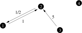
Figure 1: Weighted directed graph

Each node in this graph corresponds to an agent and each arc represents a communication channel. Each agent $i$ ($i=1,\dots,4$) is being attributed a real state variable $x_{i}\in{\mathbb{R}}$. Suppose that this weighted directed graph represents the communication pattern at time $t$. Agent $1$ receives information from agent $2$ and updates his state $x_{1}$ according to the weighted average

$$x_{1}(t+1)=\frac{1x_{1}(t)+(1/2)x_{2}(t)}{1+1/2}.$$

Notice that agent $1$’s own state $x_{1}(t)$ is taken into account with unit weight $1$. Agent $2$ receives information from agents $1$ and $3$ and updates his heading $x_{2}$ according to the weighted average

$$x_{2}(t+1)=\frac{1x_{1}(t)+1x_{2}(t)+5x_{3}(t)}{1+1+5}.$$

Agents $3$ and $4$ do not receive any information:

$$x_{3}(t+1) =x_{3}(t),$$

$$x_{4}(t+1) =x_{4}(t).$$

We are interested in the dynamics of the $x_{i}$-variables of the agents that arises when the communication graph changes over time. In order to formulate the dynamics for general graphs, we associate to a weighted directed graph ${\mathcal{G}}=({\mathcal{N}},{\mathcal{A}},w)$ with vertex set ${\mathcal{N}}=\{1,\dots,n\}$ a real $n\times n$-matrix $A({\mathcal{G}})$ whose components we define as follows:

$$(A({\mathcal{G}}))_{kl}=\begin{cases}\frac{w_{lk}}{1+\sum_{i\in{\mathrm{Neighbors}}(k,{\mathcal{A}})}w_{ik}}&\mbox{whenever $(l,k)\in{\mathcal{A}}$,}\\ \frac{1}{1+\sum_{i\in{\mathrm{Neighbors}}(k,{\mathcal{A}})}w_{ik}}&\mbox{whenever $k=l$,}\\ 0&\mbox{otherwise.}\end{cases}$$ (1)

Notice that the matrix $A({\mathcal{G}})$ is stochastic; that is, it is a square matrix with non-negative entries and with the property that its row sums are all equal to $1$. For the weighted directed graph of Fig. 1, for example, the matrix $A({\mathcal{G}})$ becomes

$$\begin{pmatrix}2/3&1/3&0&0\\ 1/7&1/7&5/7&0\\ 0&0&1&0\\ 0&0&0&1\end{pmatrix}.$$

Consider a sequence of weighted directed graphs ${\mathcal{G}}(t)=({\mathcal{N}},{\mathcal{A}}(t),w(t))$ with common vertex set ${\mathcal{N}}=\{1,\dots,n\}$ and where $t\in{\mathbb{N}}$. We are interested in the following discrete-time system on ${\mathbb{R}}^{n}$:

$$x(t+1)=A({\mathcal{G}}(t))x(t).\\$$ (2)

In particular, we want to formulate necessary and/or sufficient conditions for the convergence of the $n$ components $x_{i}(t)$ to a common value as $t\rightarrow\infty$. It is clear that the convergence properties of Eq. (2) depend both on the connectivity properties of the sequence of directed graphs and on the associated weight functions. In the present paper we focus on the role of the connectivity properties and assume that the weights are well-behaved by imposing a uniform boundedness condition. Below we state two results that follow as a consequence of the general theory established in the paper (Theorems 3 and 4). The formulation of these results relies on the notion of weak connectivity.

Definition 4 (weak connectivity).

Consider a directed graph $({\mathcal{N}},{\mathcal{A}})$. A node $k\in{\mathcal{N}}$ is connected to a node $l\in{\mathcal{N}}$ if there is a path from $k$ to $l$ in the graph which respects the orientation of the arcs. A directed graph $({\mathcal{N}},{\mathcal{A}})$ is called weakly connected if there is a node $k\in{\mathcal{N}}$ which is connected to all other nodes $l\in{\mathcal{N}}\setminus\{k\}$. A sequence of directed graphs $({\mathcal{N}},{\mathcal{A}}(t))$ with $t\in{\mathbb{N}}$ is called weakly connected across an interval $I\subseteq{\mathbb{N}}$ if the directed graph $({\mathcal{N}},\cup_{t\in I}{\mathcal{A}}(t))$ is weakly connected.

Proposition 1 (unidirectional).

Consider a sequence of weighted directed graphs ${\mathcal{G}}(t)=({\mathcal{N}},{\mathcal{A}}(t),w(t))$ with common vertex set ${\mathcal{N}}=\{1,\dots,n\}$ and where $t\in{\mathbb{N}}$. Assume the existence of $0<e_{\mathrm{min}}\leq e_{\mathrm{max}}<\infty$ such that the weight functions $w(t)$ take values in $[e_{\mathrm{min}},\,e_{\mathrm{max}}]$ for all $t\in{\mathbb{N}}$. If there is $T\geq 0$ such that for all $t_{0}\in{\mathbb{N}}$ the sequence of directed graphs $({\mathcal{N}},{\mathcal{A}}(t))$ is weakly connected across $[t_{0},\,t_{0}+T]$, then the $n$-components $\zeta_{i}(t)$ of any solution $\zeta$ of Eq. (2) converge to a common value as $t\rightarrow\infty$.

Proposition 2 (bidirectional).

Consider a sequence of weighted directed graphs ${\mathcal{G}}(t)=({\mathcal{N}},{\mathcal{A}}(t),w(t))$ with common vertex set ${\mathcal{N}}=\{1,\dots,n\}$ and where $t\in{\mathbb{N}}$. Assume the existence of $0<e_{\mathrm{min}}\leq e_{\mathrm{max}}<\infty$ such that the weight functions $w(t)$ take values in $[e_{\mathrm{min}},\,e_{\mathrm{max}}]$ for all $t\in{\mathbb{N}}$. Assume in addition that the graphs $({\mathcal{N}},{\mathcal{A}}(t))$ are bidirectional for all $t\in{\mathbb{N}}$. If for all $t_{0}\in{\mathbb{N}}$ the sequence of graphs $({\mathcal{N}},{\mathcal{A}}(t))$ is weakly connected across $[t_{0},\,\infty)$, then the $n$-components $\zeta_{i}(t)$ of any solution $\zeta$ of Eq. (2) converge to a common value as $t\rightarrow\infty$.

2.1 Discussion of Propositions 1 and 2

1. Let us mention some of the subtleties involved in the study of Eq. (2). First of all, Eq. (2) belongs to the class of linear time-varying systems, whose stability properties are hard to analyse in general. Secondly, the equilibrium value to which the components are shown to converge, is not known explicitly; this equilibrium value depends both on the initial data and on the sequence of weighted directed graphs. Thirdly, it has been shown in [8] that, in general, there does not exist a time-invariant, quadratic Lyapunov function for Eq. (2). Partially motivated by this negative result, we put forward in the present paper a series of graph-theoretic and system-theoretic analysis tools which are not based on the linear structure of Eq. (2). This contrasts our approach with the approaches taken in [8, 14] which rely heavily on linear algebra and algebraic graph theory.

2. For the special case that the weights are all equal to one, Eq. (2) reduces to the model studied in [8, Theorems 1–2]. From a control perspective, an important contribution of [8] is that this work relates the information flow and communication structure with the stability properties of the group of agents. The results obtained in the present paper generalize the results from [8, Theorems 1–2] in several directions. Apart from the observation that the present models are more general, it is important to notice that unlike [8] we do not assume bidirectional communication (Proposition 1) and, when we consider bidirectional communication, we do not assume uniformity in the connectivity condition (Proposition 2). It is rather surprising that with our inherently nonlinear approach, we are able to obtain generalizations of results recently reported in the literature, even when restricting attention to the linear case.

3. As a corollary of Proposition 1 we obtain the following graph theoretic result. A stochastic $n\times n$-matrix $A$ with positive diagonal elements has all but one of its eigenvalues strictly inside the unit circle (the only exception being the trivial eigenvalue $1$) if (and only if—see Theorem 3) the associated directed graph $({\mathcal{N}},{\mathcal{A}})$

   $${\mathcal{N}}=\{1,\dots,n\},\qquad{\mathcal{A}}=\{(k,l)\in{\mathcal{N}}\times{\mathcal{N}}:A_{lk}>0\mbox{ and }k\not=l\}$$

   is weakly connected. As before, we mention that we obtain this graph theoretic result using inherently nonlinear analysis tools. Moreover, the present approach enables us to go beyond this result by considering time-dependent stochastic matrices.

3 Multi-agent dynamics

We introduce here the dynamical equations that will be studied in the remainder of the paper. These equations model the interaction of $n$ agents via time-dependent, unidirectional communication. The individual agents share a common state space $X$ which is assumed to be finite-dimensional Euclidean. We are interested in multi-agent dynamics that guarantee convergence of the individual agents’ states to a common value. The dynamics considered in the present paper are governed by a discrete-time system on $X^{n}$. Its formulation involves two ingredients: a time-sequence of directed graphs and a discrete-time map $f$ determining the actual dynamics.

Data 1 (communication graphs).

A sequence of directed graphs $({\mathcal{N}},{\mathcal{A}}(t))$ with common node set ${\mathcal{N}}=\{1,\dots,n\}$ and with $t\in{\mathbb{N}}$;

Data 2 (discrete-time map).

A continuous function $f:{\mathbb{N}}\times X^{n}\rightarrow X^{n}$.

These ingredients give rise to the following discrete-time system on $X^{n}$

$$x(t+1)=f(t,x(t))$$ (3)

or, expressed in terms of the individual agents’ states,

$$\begin{split}x_{1}(t+1)&=f_{1}(t,x_{1}(t),\dots,x_{n}(t)),\\ &\vdots\\ x_{n}(t+1)&=f_{n}(t,x_{1}(t),\dots,x_{n}(t)).\end{split}$$

Here we have introduced the decomposition $x=(x_{1},\dots,x_{n})$ and $f=(f_{1},\dots,f_{n})$ corresponding to the product structure of $X^{n}$.

The directed graph $({\mathcal{N}},{\mathcal{A}}(t))$ characterizes the inter-agent communication at time $t$. Each node of this graph corresponds to an agent and each arc represents a communication channel. The communication graph $({\mathcal{N}},{\mathcal{A}}(t))$ determines the information that is available for the agents at time $t$ and each agent updates its state based upon this information according to Eq. (3). We impose two assumptions on the map $f=(f_{1},\dots,f_{n})$.

Assumption 1 (communication).

For every time $t\in{\mathbb{N}}$ and for each agent $k\in\{1,\dots,n\}$ the value of the function $f_{k}(t,\cdot):X^{n}\rightarrow X$ depends only on the states of agent $k$ and agents $i\in{\mathrm{Neighbors}}(k,{\mathcal{A}}(t))$; that is, $f_{k}(t,x)=f_{k}(t,\overline{x})$ whenever $x_{k}=\overline{x}_{k}$ and $x_{i}=\overline{x}_{i}$ for all $i\in{\mathrm{Neighbors}}(k,{\mathcal{A}}(t))$.

Assumption 2 (convexity).

Associated to each directed graph $({\mathcal{N}},{\mathcal{A}})$ with node set ${\mathcal{N}}=\{1,\dots,n\}$ and each agent $k$ there is a continuous set-valued function $e_{k}({\mathcal{A}}):X^{n}\rightrightarrows X$ satisfying

1. $$f_{k}(t,x)\in e_{k}({\mathcal{A}}(t))(x),\qquad\forall t\in{\mathbb{N}},\;\forall x\in X^{n};$$ (4)

2. $e_{k}({\mathcal{A}})(x_{1},\dots,x_{n})=\{x_{k}\}$ whenever the states of agent $k$ and agents $i\in{\mathrm{Neighbors}}(k,{\mathcal{A}})$ are all equal and $e_{k}({\mathcal{A}})(x_{1},\dots,x_{n})$ is contained in the relative interior of the convex hull of the states of agent $k$ and agents $i\in{\mathrm{Neighbors}}(k,{\mathcal{A}})$ whenever the states of agent $k$ and agents $i\in{\mathrm{Neighbors}}(k,{\mathcal{A}})$ are not all equal.

Remark 1.

Recall that the values of a set-valued function (from Euclidean space to Euclidean space) are, by definition, closed sets. Assumption 2 thus implies that $e_{k}({\mathcal{A}})(x_{1},\dots,x_{n})$ is a compact set contained in the relative interior of the convex hull of the states of agent $k$ and agents $i\in{\mathrm{Neighbors}}(k,{\mathcal{A}})$ whenever the states of agent $k$ and agents $i\in{\mathrm{Neighbors}}(k,{\mathcal{A}})$ are not all equal.

Assumption 1 captures the constraints that the communication topology is supposed to impose on the dynamics. Assumption 2 is a strict convexity assumption. It implies that the state $x_{k}(t+1)$ is a strict convex combination of the state $x_{k}(t)$ and the states $x_{i}(t)$ of agents $i\in{\mathrm{Neighbors}}(k,{\mathcal{A}}(t))$. Assumptions 1 and 2 are satisfied in various examples reported in the literature.

Example 1 (linear).

The linear model of Section 2 falls within the scope of the present study. Consider a sequence of weighted directed graphs ${\mathcal{G}}(t)=({\mathcal{N}},{\mathcal{A}}(t),w(t))$ with common vertex set ${\mathcal{N}}=\{1,\dots,n\}$ and where $t\in{\mathbb{N}}$. Assume the existence of $0<e_{\mathrm{min}}\leq e_{\mathrm{max}}<\infty$ such that the weight functions $w(t)$ take values in $[e_{\mathrm{min}},\,e_{\mathrm{max}}]$ for all $t\in{\mathbb{N}}$. The linear model studied in Section 2 corresponds to the case of $X={\mathbb{R}}$ and $f(t,x)=A({\mathcal{G}}(t))x$ with the matrix $A({\mathcal{G}})$ defined in Eq. (1). The discrete-time map $f$ satisfies Assumptions 1–2 with $e({\mathcal{A}})(x)$ being the set of all possible values $A({\mathcal{G}})x$ that are obtained by considering all possible weighted directed graphs ${\mathcal{G}}$ with arc set ${\mathcal{A}}$ and with weights contained in the compact interval $[e_{\mathrm{min}},\,e_{\mathrm{max}}]$.

Example 2 (synchronization).

Consider a population of oscillators that share a common state space $S^{1}$. Denote the state of oscillator $k$ by $\theta_{k}$ and consider for each communication graph $({\mathcal{N}},{\mathcal{A}})$ the Kuramoto equation [9, 16]

$$\dot{\theta}_{k}=\omega_{k}+\sum_{i\in{\mathrm{Neighbors}}(k,{\mathcal{A}})}\sin(\theta_{i}-\theta_{k}),\qquad k=1,\dots,n,$$ (5)

where we have taken the coupling strenth equal to $1$. Let us consider the case that the $\omega_{k}$ are all equal. In this case we may assume without loss of generality (by introducing a rotating reference frame) that $\omega_{1}=\dots=\omega_{n}=0$. We restrict attention to angles in the interval $(-\pi/2,\,\pi/2)$ and introduce local coordinates $(-\pi/2,\,\pi/2)\rightarrow{\mathbb{R}}:\theta_{k}\mapsto x_{k}=\tan(\theta_{k})$. Expressed in terms of these local coordinates, the Kuramoto equation becomes

$$\dot{x}_{k}=\sum_{i\in{\mathrm{Neighbors}}(k,{\mathcal{A}})}\frac{x_{i}-x_{k}}{\sqrt{1+x_{i}^{2}}\sqrt{1+x_{k}^{2}}},\qquad k=1,\dots,n.$$ (6)

The continuous-time system (6) may be studied within the present framework by introducing its time-$1$ map $\psi({\mathcal{A}}):{\mathbb{R}}^{n}\rightarrow{\mathbb{R}}^{n}$. Explicitly, consider a time-sequence $({\mathcal{N}},{\mathcal{A}}(t))$ ($t\in{\mathbb{N}}$) and put $f(t,x)=\psi({\mathcal{A}}(t))(x)$. This discrete-time map $f$ satisfies Assumptions 1 and 2 with $e({\mathcal{A}})(x)=\{\psi({\mathcal{A}})(x)\}$. Whereas most papers on synchronization restrict attention to time-independent, bidirectional coupling, the present paper allows to study synchronization of oscillators with time-varying and unidirectional coupling.

Example 3 (consensus algorithm).

The following nonlinear consensus protocol is studied in [14]. Let $X={\mathbb{R}}$ and consider for a given communication graph $({\mathcal{N}},{\mathcal{A}})$ the continuous-time system on $X^{n}$

$$\dot{x}_{k}=\sum_{i\in{\mathrm{Neighbors}}(k,{\mathcal{A}})}\gamma_{ik}(x_{i}-x_{k}),\qquad k=1,\dots,n.$$ (7)

where the functions $\gamma_{ik}:{\mathbb{R}}\rightarrow{\mathbb{R}}$ are uneven, locally Lipschitz and strictly increasing for all $(i,k)\in{\mathcal{A}}$. The continuous-time system (6) may be studied within the present framework by introducing its time-$1$ map $\psi({\mathcal{A}}):{\mathbb{R}}^{n}\rightarrow{\mathbb{R}}^{n}$. Explicitly, consider a time-sequence $({\mathcal{N}},{\mathcal{A}}(t))$ ($t\in{\mathbb{N}}$) and put $f(t,x)=\psi({\mathcal{A}}(t))(x)$. This discrete-time map $f$ satisfies Assumptions 1 and 2 with $e({\mathcal{A}})(x)=\{\psi({\mathcal{A}})(x)\}$. Whereas [14] restricts attention to time-independent and bidirectional communication graphs, the present paper allows to study nonlinear consensus protocols with time-varying and unidirectional communication.

Example 4 (swarming).

The paper [19] proposes a simple model to investigate self-ordered motion in systems of particles with biologically motivated interaction. Their model consists of a collection of particles moving with constant velocity $v$. At each time step a given particle assumes the average direction of motion of the particles in its neighborhood with some random perturbation added. Denote the direction of motion of particle $k$ by $\theta_{k}\in S^{1}$. The following model is studied in [19]

$$\theta_{k}(t+1)=\arctan\left(\frac{\sum_{i\in\{k\}\cup{\mathrm{Neighbors}}(k,{\mathcal{A}}(t))}\sin(\theta_{i}(t))}{\sum_{i\in\{k\}\cup{\mathrm{Neighbors}}(k,{\mathcal{A}}(t))}\cos(\theta_{i}(t))}\right),\qquad k=1,\dots,n,$$ (8)

where we have omitted an additive disturbance term. Here ${\mathcal{A}}(t)$ characterizes the nearest neighbor coupling at time $t$. We restrict attention to angles in the interval $(-\pi/2,\,\pi/2)$ and introduce local coordinates $(-\pi/2,\,\pi/2)\rightarrow{\mathbb{R}}:\theta_{k}\mapsto x_{k}=\tan(\theta_{k})$, as in Example 2. The model (8) expressed in terms of these local coordinates falls within the scope of the present paper. Whereas the study in [19] is based solely on simulations, the present appraoch enables us to make analytical statements about convergence.

If the headings $\theta_{k}$ are close to each other, then Eq. (8) may be approximated by the linear equation

$$x_{k}(t+1)=\sum_{i\in\{k\}\cup{\mathrm{Neighbors}}(k,{\mathcal{A}}(t))}x_{i}(t),\qquad k=1,\dots,n.$$ (9)

with $x_{k}\in{\mathbb{R}}$. This is the swarming model studied in [8] and corresponds to the linear example of Section 2 with all weights equal to $1$. Hence Eq. 9 also falls within the scope of the present paper.

Assumption 2 plays a central role in the forthcoming analysis. Its importance is already reflected in the following simple but appealing result.

Lemma 1.

Consider the Data 1–2 satisfying Assumption 2. The set-valued function $\widetilde{V}:X^{n}\rightrightarrows X$ defined for each $x=(x_{1},\dots,x_{n})\in X^{n}$ as the convex hull of $\{x_{1},\dots,x_{n}\}$, denoted by ${\mathrm{conv}}\{x_{1},\dots,x_{n}\}$, is non-increasing along the solutions of Eq. (3); that is,

$$\widetilde{V}(f(t,x))\subseteq\widetilde{V}(x)\qquad\forall t\in{\mathbb{N}},\,\forall x\in X^{n}.$$ (10)

Proof.

Assumption 2 implies

$$f_{k}(t,x)\in e_{k}({\mathcal{A}}(t))(x)\subseteq{\mathrm{conv}}\{x_{1},\dots,x_{n}\},\qquad\forall k\in\{1,\dots,n\},\;\forall t\in{\mathbb{N}},\;\forall x\in X^{n},$$ (11)

from which Eq. (10) follows immediately. ∎

Within the current framework, the statement of Lemma 1 may seem almost trivial; it arises as a straightforward consequence of Assumption 2. However, the nontrivial contribution lies precisely in the observation that many examples reported in the literature satisfy Assumption 2 and hence may be studied by means of Lemma 1. The set-valued function $\widetilde{V}$ serves as a measure for disagreement. In the forthcoming sections, we will use (a slight modification of) $\widetilde{V}$ as a set-valued Lyapunov function. The set-valued nature of the Lyapunov function turns out to be convenient as it enables the application of Lyapunov techniques in the present context, where convergence to non-isolated equilibria will be shown.

We end the section with some remarks about the limitations of the present model.

Remark 2 (non-strict convexity).

Assumption 2 is a strict convexity assumption. For some applications, it may be desirable to relax this assumption. For example, the discrete-time system

$${x}_{k}(t+1)=\max_{i\in\{k\}\cup{\mathrm{Neighbors}}(k,{\mathcal{A}}(t))}x_{i}(t),\qquad k=1,\dots,n$$ (12)

does not satisfy Assumption 2, but satisfies instead a non-strict convexity assumption: $x_{k}(t+1)$ belongs to (the boundary of) the convex hull of the state $x_{k}(t)$ and the states $x_{i}(t)$ of agents $i\in{\mathrm{Neighbors}}(k,{\mathcal{A}}(t))$. The study of dynamical equations satisfying a non-strict convexity assumption instead of Assumption 2 is beyond the scope of the present paper.

Remark 3 (non-Euclidean space).

By assuming that the common state space for the individual agents is Euclidean, we exclude some global phenomena arising, for example, in synchronization of periodic motions and in attitude allignment problems [15]. Indeed, the natural state space for the individual agents in these examples is respectively $S^{1}$ and $SO(3)$ and the global features of the dynamics that are related to the nontrivial topology of these manifolds, fall outside the scope of the present method. Nevertheless, local issues can often be studied within the present framework, for example, by introducing suitable coordinate charts. This has already been illustrated in Example 2.

4 Stability definitions

In order to enable a clear and precise formulation of the stability and convergence properties of the discrete-time system (3), we extend the familiar stability concepts of Lyapunov theory to the present framework. Notice that we are interested in the agents’ states converging to a common, constant value and that we expect this common value to depend continuously on the agents’ initial states. This means that the classical stability concepts developed for the study of individual (typically isolated) equilibria are not well-adapted to the present situation. Alternatively, one may shift attention away from the individual equilibria and consider the stability properties of the set of equilibria. However, set stability does not fully capture the convergence properties that we are aiming at. This is illustrated, for example, by the well-known phenomenon that a trajectory may converge to the set of equilibria without converging to any of the individual equilibria. The stability notions that we introduce below incorporate, among others, the requirement that all trajectories converge to one of the equilibria. We believe that the notions introduced here constitute a natural framework for questions studied in coordinated control, formation stabilization, synchronization, etc.

In the following definition we make a conceptual distinction between equilibrium solutions and equilibrium points: an equilibrium point is an element of the state space which is the constant value of an equilibrium solution. By referring explicitly to equilibrium solutions in the following definition, we distinguish the present stability concepts from the more familiar set stability concepts.

Definition 5 (stability).

Let ${\mathcal{X}}$ be a finite-dimensional Euclidean space and consider a continuous map $f:{\mathbb{N}}\times{\mathcal{X}}\rightarrow{\mathcal{X}}$ giving rise to the discrete-time system

$$x(t+1)=f(t,x(t)).$$ (13)

Consider a collection of equilibrium solutions of Eq. (13) and denote the corresponding set of equilibrium points by $\Phi$. With respect to the considered collection of equilibrium solutions, the dynamical system (13) is called

1. stable if for each $\phi_{1}\in\Phi$, for all $c_{2}>0$ and for all $t_{0}\in{\mathbb{N}}$ there is $c_{1}>0$ such that every solution $\zeta$ of Eq. (13) satisfies: if $|\zeta(t_{0})-\phi_{1}|<c_{1}$ then there is $\phi_{2}\in\Phi$ such that $|\zeta(t)-\phi_{2}|<c_{2}$ for all $t\geq t_{0}$;

2. bounded if for each $\phi_{1}\in\Phi$, for all $c_{1}>0$ and for all $t_{0}\in{\mathbb{N}}$ there is $c_{2}>0$ such that every solution $\zeta$ of Eq. (13) satisfies: if $|\zeta(t_{0})-\phi_{1}|<c_{1}$ then there is $\phi_{2}\in\Phi$ such that $|\zeta(t)-\phi_{2}|<c_{2}$ for all $t\geq t_{0}$;

3. globally attractive if for each $\phi_{1}\in\Phi$, for all $c_{1},c_{2}>0$ and for all $t_{0}\in{\mathbb{N}}$ there is $T\geq 0$ such that every solution $\zeta$ of Eq. (13) satisfies: if $|\zeta(t_{0})-\phi_{1}|<c_{1}$ then there is $\phi_{2}\in\Phi$ such that $|\zeta(t)-\phi_{2}|<c_{2}$ for all $t\geq t_{0}+T$;

4. globally asymptotically stable if it is stable, bounded and globally attractive.

Remark 4.

We may take without loss of generality $\phi_{2}=\phi_{1}$ in Items 1 and 2 of Definition 5 (but not in Item 3). Compare with the proof of Theorem 1 below. We have chosen not to incorporate $\phi_{2}=\phi_{1}$ in Items 1 and 2 in order to make the similarities with Item 3 more transparent.

Definition 5 may be interpreted as follows. Stability and boundedness require that any solution of Eq. (13) which is initially close to $\Phi$ remains close to one of the equilibria in $\Phi$, thus excluding, for example, the possibility of drift along the set $\Phi$. Global attractivity implies that every solution of Eq. (13) converges to one of the equilibria in $\Phi$. If the collection of equilibrium solutions is a singleton consisting of one equilibrium solution, then the notions of stability, boundedness, global attractivity and global asymptotic stability of Definition 5 coincide with the classical notions that have been introduced for the study of individual equilibria.

Slightly stronger stability notions result when uniformity with respect to initial time is introduced in Definition 5. If the number $c_{1}$ (respectively $c_{2}$ and $T$) may be chosen independently of $t_{0}$ in Item 1 (respectively Items 2 and 3) then the dynamical system (13) is called uniformly stable (respectively uniformly bounded and uniformly globally attractive) with respect to the considered collection of equilibrium solutions.

Theorem 1 below provides a sufficient condition for uniform stability, uniform boundedness and uniform global asymptotic stability in terms of the existence of a set-valued Lyapunov function. This result is convenient since, on the one hand, set-valued Lyapunov functions arise naturally within the present context as illustrated by Lemma 1, and on the other hand, the stability notions that are asserted in Theorem 1 are precisely those that we are aiming to prove. Apart from its application in the present paper, Theorem 1 may be of independent interest.

Theorem 1 (Lyapunov characterization).

Let ${\mathcal{X}}$ be a finite-dimensional Euclidean space and consider a continuous map $f:{\mathbb{N}}\times{\mathcal{X}}\rightarrow{\mathcal{X}}$ giving rise to the discrete-time system (13). Let $\Xi$ be a collection of equilibrium solutions of Eq. (13) and denote the corresponding set of equilibrium points by $\Phi$. Consider an upper semicontinuous set-valued function ${V}:{\mathcal{X}}\rightrightarrows{\mathcal{X}}$ satisfying

1. $x\in V(x),\qquad\forall x\in{\mathcal{X}};$

2. $V(f(t,x))\subseteq V(x),\qquad\forall t\in{\mathbb{N}},\;\forall x\in{\mathcal{X}}.$

If ${V}(\phi)=\{\phi\}$ for all $\phi\in\Phi$ then the dynamical system (13) is uniformly stable with respect to $\Xi$. If ${V}(x)$ is bounded for all $x\in{\mathcal{X}}$ then the dynamical system (13) is uniformly bounded with respect to $\Xi$.

Consider in addition a function $\mu:{\mathrm{Image}}(V)\rightarrow{\mathbb{R}}_{\geq 0}$ and a lower semicontinuous function $\beta:{\mathcal{X}}\rightarrow{\mathbb{R}}_{\geq 0}$ satisfying

1. $\mu\circ V:{\mathcal{X}}\rightarrow{\mathbb{R}}_{\geq 0}:x\mapsto\mu(V(x))$ is bounded uniformly with respect to $x$ in bounded subsets of ${\mathcal{X}}$;

2. $\beta$ is positive definite with respect to $\Phi$; that is, $\beta(\phi)=0$ for all $\phi\in\Phi$ and $\beta(x)>0$ for all $x\in{\mathcal{X}}\setminus\Phi$;

3. $\mu(V(f(t,x)))-\mu(V(x))\leq-\beta(x),\qquad\forall t\in{\mathbb{N}},\;\forall x\in{\mathcal{X}}$.

If ${V}(\phi)=\{\phi\}$ for all $\phi\in\Phi$ and ${V}(x)$ is bounded for all $x\in{\mathcal{X}}$ then the dynamical system (13) is uniformly globally asymptotically stable with respect to $\Xi$.

We briefly comment on the role of the functions $V$, $\mu$ and $\beta$ in Theorem 1. The set-valued function $V$ plays the role of a Lyapunov function which is non-increasing (decreasing) along the solutions of Eq. (13). The set-valued nature of $V$ is crucial. A set-valued function allows for a continuum of minimal elements which are not comparable with each other. For this reason, a set-valued Lyapunov function, unlike a real Lyapunov function, may be used to conclude that each trajectory converges to one equilibrium out of a continuum of equilibria. The function $\mu$ serves as a measure for the size of the values of $V$. In the present paper, we let $\mu(V(x))$ be the diameter of the set $V(x)$. The function $\beta$ characterizes the decrease of $V$ along the solutions of Eq. (13) as measured in terms of $\mu$.

Proof of Theorem 1..

(Uniform stability.) Consider arbitrary $\phi_{1}\in\Phi$ and $c_{2}>0$. If ${V}(\phi_{1})=\{\phi_{1}\}$ then, by upper semicontinuity of ${V}$, there is $c_{1}>0$ such that ${V}(x)\subset{\mathcal{B}}(\phi_{1},c_{2})$ for all $x\in{\mathcal{B}}(\phi_{1},c_{1})$. Consider arbitrary $t_{0}\in{\mathbb{N}}$ and $x_{0}\in{\mathcal{B}}(\phi_{1},c_{1})$ and let $\zeta$ denote the solution of Eq. (13) with $\zeta(t_{0})=x_{0}$. Conditions 1 and 2 of the theorem imply that

$$\zeta(t)\in V(\zeta(t))\subseteq V(x_{0})\subset{\mathcal{B}}(\phi_{1},c_{2}),\qquad\forall t\geq t_{0}.$$ (14)

(Uniform boundedness.) Consider arbitrary $\phi_{1}\in\Phi$ and $c_{1}>0$. If ${V}(x)$ is bounded for all $x\in{\mathcal{X}}$ then, by upper semicontinuity of ${V}$, there is $c_{2}>0$ such that ${V}(x)\subset{\mathcal{B}}(\phi_{1},c_{2})$ for all $x\in{\mathcal{B}}(\phi_{1},c_{1})$. Consider arbitrary $t_{0}\in{\mathbb{N}}$ and $x_{0}\in{\mathcal{B}}(\phi_{1},c_{1})$ and let $\zeta$ denote the solution of Eq. (13) with $\zeta(t_{0})=x_{0}$. Conditions 1 and 2 of the theorem imply that

$$\zeta(t)\in V(\zeta(t))\subseteq V(x_{0})\subset{\mathcal{B}}(\phi_{1},c_{2}),\qquad\forall t\geq t_{0}.$$ (15)

(Uniform global asymptotic stability.) We have already proved that, if ${V}(\phi)=\{\phi\}$ for all $\phi\in\Phi$ and ${V}(x)$ is bounded for all $x\in{\mathcal{X}}$, then the dynamical system (13) is uniformly stable and uniformly bounded with respect to $\Xi$. It remains to prove uniform global attractivity with respect to $\Xi$.

Consider arbitrary $\phi_{1}\in\Phi$ and $c_{1}>0$. If ${V}(x)$ is bounded for all $x\in{\mathcal{X}}$ then, by upper semicontinuity of ${V}$, there is a compact set $K\subset{\mathcal{X}}$ such that ${V}(x)\subseteq K$ for all $x\in{\mathcal{B}}(\phi_{1},c_{1})$. Similarly as above, Conditions 1 and 2 of the theorem imply that every solution of Eq. (13) initiated in ${\mathcal{B}}(\phi_{1},c_{1})$ remains in $K$.

Consider in addition arbitrary $c_{2}>0$. If ${V}(\phi)=\{\phi\}$ for all $\phi\in\Phi$ then, by upper semicontinuity of ${V}$, there is $c_{3}>0$ such that for all $x\in{\mathcal{B}}(\Phi\cap K,c_{3})$ there is $\phi_{2}\in\Phi$ such that ${V}(x)\subset{\mathcal{B}}(\phi_{2},c_{2})$. Similarly as above, Conditions 1 and 2 of the theorem imply that every solution of Eq. (13) entering ${\mathcal{B}}(\Phi\cap K,c_{3})$ remains in a $c_{2}$-ball around some equilibrium point $\phi_{2}\in\Phi$.

It remains to prove the existence of $T\geq 0$ such that every solution of Eq. (13) starting in ${\mathcal{B}}(\phi_{1},c_{1})$ cannot remain longer than $T$ subsequent times in $K$ without entering ${\mathcal{B}}(\Phi\cap K,c_{3})$. In agreement with Conditions 3 and 4 of the theorem and the lower semicontinuity of $\beta$, we introduce two real numbers

$$M=\sup_{x\in{{\mathcal{B}}(\phi_{1},c_{1})}}\mu(V(x))<\infty$$

and

$$\Delta=\min_{x\in K\setminus{\mathcal{B}}(\Phi,c_{3})}\beta(x)>0.$$

Let $T\geq 0$ be such that $T\Delta>M$. Consider arbitrary $t_{0}\in{\mathbb{N}}$ and $x_{0}\in{\mathcal{B}}(\phi_{1},c_{1})$ and let $\zeta$ denote the solution of Eq. (13) with $\zeta(t_{0})=x_{0}$. Then Condition 5 of the theorem implies that for some $t_{1}\in[t_{0},\,t_{0}+T]$

$$\zeta(t_{1})\in{\mathcal{B}}(\Phi\cap K,c_{3}),$$

since otherwise $\mu(V(\zeta(t_{0}+T)))$ would be smaller than zero, contradicting that $\mu$ takes only non-negative values. Putting everything together, we conclude that for some $\phi_{2}\in\Phi$

$$\zeta(t)\in V(\zeta(t))\subseteq V(\zeta(t_{1}))\subset{\mathcal{B}}(\phi_{2},c_{2}),\qquad\forall t\geq t_{0}+T.$$ (16)

∎

Remark 5.

The strict decrease condition (Condition 5) of Theorem 1 may be considerably relaxed. Consider, for example, the following condition which requires that $\mu\circ V$ decreases over time-intervals of length $\tau$

1. There is a time $\tau\in{\mathbb{N}}$ such that

   $$\mu(V(f(t+\tau-1,\dots f(t+1,f(t,x))\dots)))-\mu(V(x))\leq-\beta(x),\qquad\forall t\in{\mathbb{N}},\;\forall x\in{\mathcal{X}}.$$ (17)

Theorem 1 is still true if Condition 5 is replaced by Condition 6.

Remark 6.

The Lyapunov functions featuring in Theorem 1 are set-valued functions $V:{\mathcal{X}}\rightrightarrows{\mathcal{X}}$, or equivalently, single-valued functions $V:{\mathcal{X}}\rightarrow{\mathcal{P}}({\mathcal{X}})$. One may be interested in generalizations of Theorem 1 considering more abstract Lyapunov functions $V:{\mathcal{X}}\rightarrow Z$ with $Z$ not necessarily equal to ${\mathcal{P}}({\mathcal{X}})$. The determination of appropriate structures and properties for the set $Z$ and the function $V$ enabling Lyapunov-type of results is beyond the scope of this study. Nevertheless, we point out that a partial ordering of the set $Z$ seems to be an essential ingredient in order to be able to conclude that every solution converges to one equilibrium out of a continuum of equilibria. It turns out that the class of set-valued functions $V:{\mathcal{X}}\rightrightarrows{\mathcal{X}}$ is universal in this context, in the following sense. Consider a set $Z$ and let $\prec$ by a strict partial ordering of $Z$. Consider a set ${\mathcal{X}}$ and a function $\widetilde{V}:{\mathcal{X}}\rightarrow Z$. Introduce for every $x\in{\mathcal{X}}$ the subset $V(x)\subseteq{\mathcal{X}}$ defined by

$${V}(x)=\{\hat{x}\in{\mathcal{X}}:\widetilde{V}(\hat{x})\prec\widetilde{V}(x)\mbox{ or }\widetilde{V}(\hat{x})=\widetilde{V}(x)\}.$$

Then we have ${V}(x)={V}(\overline{x})$ whenever $\widetilde{V}(x)=\widetilde{V}(\overline{x})$ and ${V}(x)\subset{V}(\overline{x})$ whenever $\widetilde{V}(x)\prec\widetilde{V}(\overline{x})$. The proof of this statement is elementary and therefore omitted. Not only does this result provide some motivation for restricting attention to set-valued maps $V:{\mathcal{X}}\rightrightarrows{\mathcal{X}}$ in Theorem 1, it also points towards a constructive method for finding such set-valued Lyapunov functions. See, for example, the proof of Theorem 2.

We have the following consequence of Theorem 1 and Lemma 1.

Theorem 2.

Consider the Data 1–2 satisfying Assumption 2. The discrete-time system (3) is uniformly stable and uniformly bounded with respect to the collection of equilibrium solutions $x_{1}(t)\equiv\dots\equiv x_{n}(t)\equiv\mathrm{constant}$.

Proof of Theorem 2.

In order to apply Theorem 1 we introduce the set-valued function ${V}:{X^{n}}\rightrightarrows{X^{n}}$ according to

$$V(x_{1},\dots,x_{n})=({\mathrm{conv}}\{x_{1},\dots,x_{n}\})^{n},\qquad\forall x\in{X^{n}}.$$

The set-valued function $V$ is derived from $\widetilde{V}$ following the procedure of Remark 6 with ${\mathcal{P}}(X),\subset$ playing the role of $Z,\prec$. The set-valued function $V$ is easily seen to be globally Lipschitz. Theorem 2 follows immediately from Theorem 1 and Lemma 1. ∎

5 Uniform global attractivity

Contrary to what might be expected from Lemma 1 or Theorem 2, the dynamics of Eq. (3) may be surprisingly complex. For example, the agents’ states may fail to converge to a common value, even in the presence of inter-agent communication. In the remainder of the paper, a blend of graph-theoretic and system-theoretic tools will be used in order to establish necessary and/or sufficient conditions for global attractivity.

In the present section we restrict attention to global attractivity uniform with respect to initial time. We provide a necessary and sufficient condition for uniform global attractivity of Eq. (3). The condition that we present does not involve the actual discrete-time map $f$; it only involves the sequence of communication graphs $({\mathcal{N}},{\mathcal{A}}(t))$.

Theorem 3 (uniform global attractivity).

Consider the Data 1–2 satisfying Assumptions 1–2. The discrete-time system (3) is uniformly globally attractive with respect to the collection of equilibrium solutions $x_{1}(t)\equiv\dots\equiv x_{n}(t)\equiv\mathrm{constant}$ if and only if there is $T\geq 0$ such that for all $t_{0}\in{\mathbb{N}}$ the sequence of communication graphs is weakly connected across $[t_{0},\,t_{0}+T]$.

Proof of Theorem 3.

(Only if, proof by contraposition.) Assume that for every $T\geq 0$ there is $t_{0}\in{\mathbb{N}}$ such that the sequence of communication graphs is not weakly connected across $[t_{0},\,t_{0}+T]$. By Theorem 5 in the Appendix, this implies that for every $T\geq 0$ there is $t_{0}\in{\mathbb{N}}$ and there are nonempty, disjoint subsets ${\mathcal{L}}_{1},{\mathcal{L}}_{2}\subset{\mathcal{N}}$ such that ${\mathrm{Neighbors}}({\mathcal{L}}_{1},{\mathcal{A}}(t))$ and ${\mathrm{Neighbors}}({\mathcal{L}}_{2},{\mathcal{A}}(t))$ are both empty for all $t\in[t_{0},\,t_{0}+T]$. Pick two different elements $y,\overline{y}\in X$ and consider any solution $\zeta$ of Eq. (3) with initial data

$$\zeta_{j}(t_{0})\begin{cases}=y&\quad\forall j\in{\mathcal{L}}_{1},\\ =\overline{y}&\quad\forall j\in{\mathcal{L}}_{2},\\ \in{\mathrm{conv}}\{y,\overline{y}\}&\quad\forall j\in{\mathcal{N}}\setminus({\mathcal{L}}_{1}\cup{\mathcal{L}}_{2}).\end{cases}$$ (18)

Assumption 2 implies that, at time $t_{0}+T+1$, we still have

$$\zeta_{j}(t_{0}+T+1)\begin{cases}=y&\quad\forall j\in{\mathcal{L}}_{1},\\ =\overline{y}&\quad\forall j\in{\mathcal{L}}_{2},\\ \in{\mathrm{conv}}\{y,\overline{y}\}&\quad\forall j\in{\mathcal{N}}\setminus({\mathcal{L}}_{1}\cup{\mathcal{L}}_{2}),\end{cases}$$ (19)

since ${\mathrm{Neighbors}}({\mathcal{L}}_{1},{\mathcal{A}}(t))$ and ${\mathrm{Neighbors}}({\mathcal{L}}_{2},{\mathcal{A}}(t))$ are both empty for all $t\in[t_{0},\,t_{0}+T]$. As the time $T$ may be chosen arbitrarily large, it is not difficult to see that this contradicts uniform global attractivity of Eq. (3) with respect to the equilibrium solutions $x_{1}(t)\equiv\dots\equiv x_{n}(t)\equiv\mathrm{constant}$.

(If.) Let $T\geq 0$ be such that for all $t_{0}\in{\mathbb{N}}$ the sequence of communication graphs is weakly connected across $[t_{0},\,t_{0}+T]$. Consider an arbitrary solution $\zeta$ of Eq. (3) and an arbitrary time $t_{0}\in{\mathbb{N}}$ and assume that the $\zeta_{j}(t_{0})$’s ($j\in{\mathcal{N}}$) are not all equal. We first show that ${\widetilde{V}}(\zeta(t_{0}+(n-1)(T+1)))$ is strictly contained in ${\widetilde{V}}(\zeta(t_{0}))$, where ${\widetilde{V}}$ is the set-valued function introduced in Lemma 1.

In order to show this, we introduce a number of auxiliary functions. Denote the $m$ vertices ($2\leq m\leq n$) of the polytope ${\widetilde{V}}(\zeta(t_{0}))$ by $y_{1},\dots,y_{m}\in X$. Associate to each vertex $y_{i}$ the set-valued function $a_{i}:[t_{0},\,\infty)\rightrightarrows{\mathcal{N}}$ identifying the agents located at that vertex:

$$a_{i}(t)=\{j\in{\mathcal{N}}:\zeta_{j}(t)=y_{i}\},\qquad\forall t\in[t_{0},\,\infty),\,\forall i=1,\dots,m.$$ (20)

The strict convexity assumption (Assumption 2) implies that an agent which is not located at a vertex $y_{i}$ at some time $t\geq t_{0}$ can never reach this vertex in finite time:

$$a_{i}(t+1)\subseteq a_{i}(t),\qquad\forall t\in[t_{0},\,\infty),\,\forall i=1,\dots,m.$$ (21)

We now establish a strict decrease property for the functions $a_{i}$. We show that, under the connectivity assumption of the theorem, at least $m-1$ of the functions $a_{1},\dots,a_{m}$ are empty-valued at $t=t_{0}+(n-1)(T+1)$. Consider any intermediate time interval $[t_{0}+p(T+1),\,t_{0}+p(T+1)+T]$ ($p=0,\dots,n-2$). The assumption of the theorem implies the existence of an agent $k$ which is connected to all other agents across $[t_{0}+p(T+1),\,t_{0}+p(T+1)+T]$. We distinguish two cases.

1. If agent $k$ is located in one of the vertices at time $t_{0}+p(T+1)$; that is, if there is $i\in\{1,\dots,m\}$ such that $k\in a_{i}(t_{0}+p(T+1))$, then all the other vertices $j\in\{1,\dots,m\}\setminus\{i\}$ where agents are located at time $t_{0}+p(T+1)$ (that is, $a_{j}(t_{0}+p(T+1))\not=\emptyset$) satisfy the following: ${\mathrm{Neighbors}}(a_{j}(t_{0}+p(T+1)),{\mathcal{A}}(t))\not=\emptyset$ for some $t\in[t_{0}+p(T+1),\,t_{0}+p(T+1)+T]$ and hence, by the strict convexity assumption (Assumption 2), $a_{j}(t_{0}+(p+1)(T+1))$ is strictly contained in $a_{j}(t_{0}+p(T+1))$.

2. If agent $k$ is not located in one of the vertices at time $t_{0}+p(T+1)$; that is, if $k\notin a_{j}(t_{0}+p(T+1))$ for all $j\in\{1,\dots,m\}$, then all vertices $j\in\{1,\dots,m\}$ where agents are located at time $t_{0}+p(T+1)$ (that is, $a_{j}(t_{0}+p(T+1))\not=\emptyset$) satisfy the following: ${\mathrm{Neighbors}}(a_{j}(t_{0}+p(T+1)),{\mathcal{A}}(t))\not=\emptyset$ for some $t\in[t_{0}+p(T+1),\,t_{0}+p(T+1)+T]$ and hence, by the strict convexity assumption (Assumption 2), $a_{j}(t_{0}+(p+1)(T+1))$ is strictly contained in $a_{j}(t_{0}+p(T+1))$.

Since the above argument holds for every time interval $[t_{0}+p(T+1),\,t_{0}+p(T+1)+T]$ ($p=0,\dots,n-2$) and since the maximum number of agents at each vertex at time $t_{0}$ is not greater than $n-1$, we may thus conclude that at least $m-1$ of the functions $a_{1},\dots,a_{m}$ are empty-valued at $t=t_{0}+(n-1)(T+1)$. This establishes a strong decrease property for the set-valued function ${\widetilde{V}}$. The polytope ${\widetilde{V}}(\zeta(t_{0}+(n-1)(T+1)))$ is strictly contained in the polytope ${\widetilde{V}}(\zeta(t_{0}))$ and both sets have not more than one vertex in common.

In order to prepare for an application of Theorem 1, we introduce the set-valued function $V:{{X^{n}}}\rightrightarrows{X^{n}}$ according to

$$V(x_{1},\dots,x_{n})=({\mathrm{conv}}\{x_{1},\dots,x_{n}\})^{n},\qquad\forall t\in{\mathbb{N}},\;\forall x\in{X^{n}},$$

similarly as in the proof of Theorem 2. In addition we also introduce a real-valued function $\beta:{X^{n}}\rightarrow{\mathbb{R}}$ according to

$$\beta(x)=\inf_{\zeta_{0},\dots,\zeta_{\tau}}\mu(V(\zeta_{0}))-\mu(V(\zeta_{\tau})),\qquad\tau=(n-1)(T+1)$$ (22)

where $\mu$ denotes the diameter of a set and where the infimum is taken over all sequences $\zeta_{0},\dots,\zeta_{\tau}$ in $X^{n}$ satisfying

$$\begin{split}\zeta_{0}&=x,\\ \zeta_{1}&\in e({\mathcal{A}}(t_{0}))(\zeta_{0}),\\ &\vdots\\ \zeta_{\tau}&\in e({\mathcal{A}}(t_{0}+\tau-1))(\zeta_{\tau-1}),\end{split}$$ (23)

for some $t_{0}\in{\mathbb{N}}$. The $\zeta_{i}$ may be interpreted as the states that are possibly reachable from $x$ in $i$ time steps according to Assumption 2.

We establish some useful properties of $\beta$. First, the collection of all sequences $\zeta_{0},\dots,\zeta_{\tau}$ in $X^{n}$ satisfying (23) for some $t_{0}\in{\mathbb{N}}$

• is nonempty and compact for all $x\in X^{n}$;

• depends continuously on $x$.

This follows from the observations that the set-valued functions $e({\mathcal{A}}):X^{n}\rightrightarrows X^{n}$ are continuous and take nonempty, compact values (implied by Assumption 2) and that there is only a finite number of possible sequences of $\tau$ communication graphs. Secondly, the expression $\mu(V(\zeta_{0}))-\mu(V(\zeta_{\tau}))$ being minimized in (22)

• depends continuously on $\zeta_{0}$ and $\zeta_{\tau}$: indeed, this follows from the global Lipschitz character of $V$;

• is zero whenever the $n$ components of $x$ are all equal: indeed, in this case Assumption 2 implies that $\zeta_{0}=\dots=\zeta_{\tau}=x$ is the only sequence satisfying (23) for some $t_{0}\in{\mathbb{N}}$;

• is strictly positive whenever the $n$ components of $x$ are not all equal: indeed, this follows from the strict decrease property of $\widetilde{V}$ that has been established above and the observation that $V(x)=(\widetilde{V}(x))^{n}$.

Putting all elements together, we conclude that the function $\beta:{X^{n}}\rightarrow{\mathbb{R}}$ is continuous and positive definite with respect to $\{(x_{1},\dots,x_{n})\in X^{n}:x_{1}=\dots=x_{n}\}$.

The proof is concluded with an application of Theorem 1 (see Remark 5) which establishes uniform global asymptotic stability of Eq. (3). ∎

6 Non-uniform global attractivity

The previous section has presented a necessary and sufficient condition for uniform global attractivity. Not surprisingly, this necessary and sufficient condition involves a connectivity requirement on the sequence of directed graphs, uniform with respect to initial time. In the present section, we turn attention to global attractivity, not necessarily uniform with respect to initial time. Unlike the previous section, where the situation is quite clear, the study of non-uniform attractivity turns out to be much more subtle. We start with a necessary condition for global attractivity, not necessarily uniform with respect to time.

Proposition 3 (global attractivity).

Consider the Data 1–2 satisfying Assumptions 1–2. Global attractivity of the discrete-time system (3) with respect to the collection of equilibrium solutions $x_{1}(t)\equiv\dots\equiv x_{n}(t)\equiv\mathrm{constant}$ implies that for all $t_{0}\in{\mathbb{N}}$ the sequence of communication graphs is weakly connected across $[t_{0},\,\infty)$.

The proof of Proposition 3 is very similar to the proof of the only if-part of Theorem 3 and is omitted. The necessary condition featuring in Proposition 3 may be interpreted as a non-uniform version of the necessary and sufficient condition featuring in Theorem 3. It may therefore seem tempting to conjecture that this necessary condition is also sufficient for global attractivity, not necessarily uniform with respect to time. However, the following counterexample shows that this is not the case.

6.1 Counterexample

The counterexample is concerned with three agents sharing a common state space $X={\mathbb{R}}$. Among all possible directed graphs on the vertex set $\{1,2,3\}$ we consider

$$\begin{split}{\mathcal{A}}_{\mathrm{a}}&=\{(1,2)\},\\ {\mathcal{A}}_{\mathrm{b}}&=\{(1,2),(2,1)\},\\ {\mathcal{A}}_{\mathrm{c}}&=\{(3,2)\},\\ {\mathcal{A}}_{\mathrm{d}}&=\{(2,3),(3,2)\}.\end{split}$$ (24)

We will introduce a sequence of directed graphs which consists of the concatenation of finite sequences of the form $B_{s}$ ($s\in\{0\}\cup{\mathbb{N}}$):

$$B_{s}=\underset{2s}{\underbrace{{\mathcal{A}}_{\mathrm{a}},\dots,{\mathcal{A}}_{\mathrm{a}}}},{\mathcal{A}}_{\mathrm{b}},\underset{2s+1}{\underbrace{{\mathcal{A}}_{\mathrm{c}},\dots,{\mathcal{A}}_{\mathrm{c}}}},{\mathcal{A}}_{\mathrm{d}}.$$

Proposition 4.

Let the number of agents be given by $n=3$ and consider the sequence of communication graphs $({\mathcal{N}},{\mathcal{A}}(t))$ with $t\in{\mathbb{N}}$ corresponding to the concatenation $B_{0},B_{1},B_{2},B_{3},\dots$ Let the common state space for the individual agents be given by $X={\mathbb{R}}$ and consider the discrete-time map $f$ corresponding to the linear example of Section 2 with all the weights equal to one. Let $\zeta$ be the solution of Eq. (3) with initial data $\zeta_{1}(1)=0$ and $\zeta_{2}(1)=\zeta_{3}(1)=1$. Then the three components of $\zeta(t)$ do not converge to a common value as $t\rightarrow\infty$.

Proof.

In order to show that the three components of $\zeta(t)$ do not converge to a common value as $t\rightarrow\infty$, we evaluate the difference $\zeta_{3}-\zeta_{1}$ at the sequence of time-instants $t_{1},t_{2},t_{3},\dots\rightarrow\infty$ determined by $t_{p+1}-t_{p}=p+1$ for all $p\in{\mathbb{N}}$ and $t_{1}=2$ (Fig. 2).

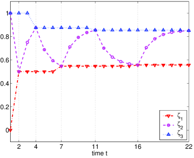
Figure 2: Counterexample

For the ease of notation, let us denote $\zeta_{3}(t_{p})-\zeta_{1}(t_{p})$ by $v(p)$. It is not difficult to see that

$$v(p+1) =v(p)-\frac{1}{2^{p+1}}v(p)=\frac{2^{p+1}-1}{2^{p+1}}v(p),\qquad\forall p\in{\mathbb{N}},$$ (25)

$$v(1) =1/2,$$ (26)

from which it follows that $0<v(p)<1$ for all $p\in{\mathbb{N}}$. Clearly $v(p)$ is decreasing with $p$ and converges to a limit as $p\rightarrow\infty$. The total accumulative decrease of $v$ satisfies

$$\sum_{p=1}^{\infty}\big{(}v(p)-v(p+1)\big{)} =\sum_{p=1}^{\infty}\frac{1}{2^{p+1}}v(p)$$ (27)

$$<\sum_{p=1}^{\infty}\frac{1}{2^{p+1}}=\frac{1}{2},$$ (28)

where we have used the recursive relation (25) and the observation that $0<v(p)<1$ for all $p\in{\mathbb{N}}$. Since $v(1)=1/2$ we conclude that

$$\lim_{p\rightarrow\infty}\zeta_{3}(t_{p})-\zeta_{1}(t_{p})=\lim_{p\rightarrow\infty}v(p)=v(1)-\sum_{p=1}^{\infty}\big{(}v(p)-v(p+1)\big{)}>0.$$ (29)

∎

6.2 Discussion of counterexample

1. First of all, notice that the sequence of directed graphs featuring in the counterexample satisfies the necessary condition of Proposition 3. The union of the arc sets ${\mathcal{A}}(t)$ over any interval of the form $[t_{0},\,\infty)$ is given by $\{(1,2),(2,1),(2,3),(3,2)\}$ which corresponds to a connected, bidirectional graph. This counterexample thus clearly shows that the necessary condition of Proposition 3 is not sufficient for global attractivity.

2. The counterexample points towards a non-intuitive phenomenon, namely that more information exchange does not necessarily lead to improved convergence properties, and may eventually even destroy convergence of the agents’ states to a common value. To be more precise, if we replace the arc sets ${\mathcal{A}}_{\mathrm{a}}$ and ${\mathcal{A}}_{\mathrm{c}}$ by the empty set, which results in reduced communication, then the discrete-time system featuring in Proposition 4 becomes globally attractive. By taking ${\mathcal{A}}_{\mathrm{a}}$ and ${\mathcal{A}}_{\mathrm{c}}$ as defined in (24) instead of the empty set, which increases the communication, the agents’ states fail to converge to a common value. It is, of course, well-known that more feedback does not necessarily mean improved convergence, but we are inclined to believe that the present phenomenon is different from previously observed, similar phenomena. To illustrate this, let us note that the loss of convergence observed in the counterexample can only occur in the context of time-dependent and unidirectional communication (see Theorem 3 and Theorem 4 of the next section).

7 Bidirectional communication

The study of global attractivity of Eq. (3), not necessarily uniform with respect to initial time, is simplified considerably when bidirectional communication is assumed.

Theorem 4 (bidirectional).

Consider the Data 1–2 satisfying Assumptions 1–2. Assume in addition that the communication graphs $({\mathcal{N}},{\mathcal{A}}(t))$ are bidirectional for all $t\in{\mathbb{N}}$. The discrete-time system (3) is globally attractive with respect to the collection of equilibrium solutions $x_{1}(t)\equiv\dots\equiv x_{n}(t)\equiv\mathrm{constant}$ if and only if for all $t_{0}\in{\mathbb{N}}$ the sequence of bidirectional graphs $({\mathcal{N}},{\mathcal{A}}(t))$ is connected across $[t_{0},\,\infty)$.

The proof of Theorem 4 is based on an analysis of $\omega$-limit sets. It is, of course, well-known that $\omega$-limit sets play a central role in the stability analysis of dynamical systems through the celebrated LaSalle principle, but it is quite remarkable that the notion of $\omega$-limit set proves to be useful in the present context, since we are considering time-varying dynamical systems, not necessarily periodic.

Proof of Theorem 4.

(Only if.) This follows from Proposition 3 and the observation that a bidirectional graph is connected if and only if it is weakly connected.

(If.) It suffices to prove that every solution of Eq. (3) converges to one of the equilibrium solutions $x_{1}(t)\equiv\dots\equiv x_{n}(t)\equiv\mathrm{constant}$. Indeed, by continuity and compactness arguments, convergence of all individual solutions actually implies global attractivity in the sense of Definition 5. The observation that compactness may be invoked is not trivial (since the set of equilibrium points is unbounded) but follows from the boundedness property of Eq. (3) established in Theorem 2.

In the remainder of the proof we show that every solution of Eq. (3) converges to one of the equilibrium solutions $x_{1}(t)\equiv\dots\equiv x_{n}(t)\equiv\mathrm{constant}$. Consider arbitrary $t_{0}\in{\mathbb{N}}$ and $x_{0}\in{X^{n}}$, and let $\zeta$ denote the solution of Eq. (3) with initial data $\zeta(t_{0})=x_{0}$. Let $\Omega$ denote the $\omega$-limit set of $\zeta$. We start with observing that

$$\widetilde{V}(x)=\widetilde{V}(\overline{x}),\qquad\forall x,\overline{x}\in\Omega,$$ (30)

where $\widetilde{V}$ is the set-valued function introduced in Lemma 1. Indeed, the existence of $x,\overline{x}\in\Omega$ with $\widetilde{V}(x)\not=\widetilde{V}(\overline{x})$ would contradict the non-increase property established in Lemma 1. We denote the constant value of $\widetilde{V}$ on $\Omega$ by $\widetilde{V}(\Omega)$.

Clearly, in order to establish that $\zeta$ converges to one of the equilibrium solutions $x_{1}(t)\equiv\dots\equiv x_{n}(t)\equiv\mathrm{constant}$, it suffices to prove that $\widetilde{V}(\Omega)$ is a singleton. We prove this by contradiction. Assume that $\widetilde{V}(\Omega)$ is not a singleton. In this case, $\widetilde{V}(\Omega)$ is a polytope with $m$ vertices ($2\leq m\leq n$) which we denote by $y_{1},\dots,y_{m}\in X$. We associate to each vertex $y_{i}$ a set-valued function $b_{i}:{X^{n}}\rightrightarrows{\mathcal{N}}$ identifying the agents located at that vertex:

$$b_{i}(x)=\{j\in{\mathcal{N}}:x_{j}=y_{i}\},\qquad\forall x\in{X^{n}},\,\forall i=1,\dots,m.$$ (31)

Observation (30) implies that

$$b_{i}(x)\not=\emptyset,\qquad\forall x\in\Omega,\,\forall i=1,\dots,m.$$ (32)

We arrive at a contradiction with the aid of the following result.

Claim 1.

If the connectivity condition mentioned in Theorem 4 holds, then for every $x\in\Omega$ with $b_{i}(x)\not=\emptyset$ for all $i\in\{1,\dots,m\}$ there exists $\overline{x}\in\Omega$ with $b_{i}(\overline{x})$ strictly contained in $b_{i}(x)$ for some $i\in\{1,\dots,m\}$.

Indeed, a repetitive application of this result eventually leads to the existence of $x^{*}\in\Omega$ with $b_{i}(x^{*})=\emptyset$ for some $i\in\{1,\dots,m\}$, contradicting (32). We have thus shown, by contradiction, that $\widetilde{V}(\Omega)$ is a singleton and thus that $\zeta$ converges to one of the equilibrium solutions $x_{1}(t)\equiv\dots\equiv x_{n}(t)\equiv\mathrm{constant}$.

We end the proof of Theorem 4 with a proof of Claim 1. Consider an arbitrary $x\in\Omega$ with $b_{i}(x)\not=\emptyset$ for all $i\in\{1,\dots,m\}$. There is, by definition, a sequence of times $t_{q}$ ($q\in{\mathbb{N}}$) tending to infinity such that $\zeta(t_{q})\rightarrow x$ as $q\rightarrow\infty$. Based upon the sequence of times $t_{q}$ we construct another sequence of times $\hat{t}_{q}$ ($q\in{\mathbb{N}}$) tending to infinity, as follows. Let for each $q\in{\mathbb{N}}$ the time $\hat{t}_{q}$ be defined as the first time greater than or equal to $t_{q}$ at which communication occurs between an agent $k\in b_{i}(x)$ and an agent $l\not\in b_{i}(x)$ for some $i\in\{1,\dots,m\}$:

$$\hat{t}_{q}=\min\{t\in[t_{q},\,\infty):{\mathrm{Neighbors}}(b_{i}(x),{\mathcal{A}}(t))\not=\emptyset\mbox{ for some~{}$i=1,\dots,m$}\},\qquad\forall q\in{\mathbb{N}}.$$

The validity of this construction follows from the connectivity condition of Theorem 4 that we are assuming to hold. We may assume without loss of generality (by considering an appropriate subsequence if necessary) that

1. the $\zeta(\hat{t}_{q})$ converge to a limit point $\hat{x}\in\Omega$ as $q\rightarrow\infty$ (by boundedness of the solution $\zeta$);

2. the ${\mathcal{A}}(\hat{t}_{q})$ are all equal, say, ${\mathcal{A}}(\hat{t}_{q})=\widehat{{\mathcal{A}}}$ for all $q\in{\mathbb{N}}$ (since there is only a finite number of possible communication graphs);

3. the $\zeta(\hat{t}_{q}+1)$ converge to a limit point $\overline{x}\in\Omega$ as $q\rightarrow\infty$ (by continuity of the set-valued map $e(\widehat{{\mathcal{A}}})$ and compactness of $e(\widehat{{\mathcal{A}}})(\hat{x})$ implied by Assumption 2).

It follows that $\overline{x}\in e(\widehat{{\mathcal{A}}})(\hat{x})$. By construction of the sequence of times $\hat{t}_{q}$ we conclude that, on the one hand, $b_{i}(\hat{x})=b_{i}(x)$ for all $i\in\{1,\dots,m\}$, and, on the other hand, $b_{i}(\overline{x})$ is strictly contained in $b_{i}(\hat{x})$ for some $i\in\{1,\dots,m\}$ (by Assumption 2). This concludes the proof of claim 1 and hence also of Theorem 4. ∎

8 Conclusion

We have considered in the paper a simple but appealing model for $n$ interacting agents via unidirectional and time-dependent communication. This model finds wide application in a variety of fields including synchronization, swarming and distributed decision making. In the model, each agent updates his state based upon the information received from other agents, according to a simple rule. By considering simple dynamics for the individual agents, we are able to focus on the main aspects of communication topology without having to deal with the additional complications arising from complex dynamical agents.

The analysis starts with the assumption that each agent updates his state according to a strict convex combination of its neighbors’ states, an assumption which is satisfied in various examples studied in the literature. This assumption leads to the development of a set-valued Lyapunov theory, with the convex hull of the individual agents’ states playing the role of a non-increasing Lyapunov function. Contrary to what might be expected, the dynamics of the multi-agent system turns out to be quite subtle and a blend of graph-theoretic and system theoretic tools is used in order to obtain necessary and/or sufficient conditions for convergence.

The strongest result is obtained for the case of bidirectional communication. In that case, it is shown that convergence of the individual agents’ states to a common value is guaranteed if, during each interval of the form $[t_{0},\infty)$, each agent sends information to each other agent, either through direct communication or indirectly via intermediate agents.

The case of unidirectional communication is more subtle. It is shown by means of a counterexample that, contrary to what might be expected, convergence of the individual agents’ states to a common value is not necessarily guaranteed, even if during each interval of the form $[t_{0},\infty)$ there is an agent who sends information to all other agents, either through direct communication or indirectly via intermediate agents. Convergence is proven, however, if a uniform bound is imposed on the time it takes for the information to spread over the network.

The counterexample that is used to show that the agents’ states may fail to converge to a common value, even in the presence of communication, points towards a counter-intuitive phenomenon. Namely that more information exchange does not necessarily lead to improved convergence and may eventually even lead to a loss of convergence, even for the simple models studied in the present paper. The study of the quantitative relationship between communication topology and speed of convergence remains an interesting area of further research.

Appendix A Graph-theoretic result

Theorem 5.

A directed graph $({\mathcal{N}},{\mathcal{A}})$ is weakly connected if and only if every pair of nonempty, disjoint subsets ${\mathcal{L}}_{1},{\mathcal{L}}_{2}\subset{\mathcal{N}}$ satisfies ${\mathrm{Neighbors}}({\mathcal{L}}_{1},{\mathcal{A}})\cup{\mathrm{Neighbors}}({\mathcal{L}}_{2},{\mathcal{A}})\not=\emptyset$.

Proof.

(Only if.) Assume that the node $k$ is connected to all other nodes, and consider an arbitrary pair of nonempty, disjoint subsets ${\mathcal{L}}_{1},{\mathcal{L}}_{2}\subset{\mathcal{N}}$. We distinguish three cases.

1. If $k\in{\mathcal{L}}_{1}$ then ${\mathrm{Neighbors}}({\mathcal{L}}_{2},{\mathcal{A}})$ is nonempty.

2. If $k\in{\mathcal{L}}_{2}$ then ${\mathrm{Neighbors}}({\mathcal{L}}_{1},{\mathcal{A}})$ is nonempty.

3. If $k\notin{\mathcal{L}}_{1}\cup{\mathcal{L}}_{2}$ then ${\mathrm{Neighbors}}({\mathcal{L}}_{1},{\mathcal{A}})$ and ${\mathrm{Neighbors}}({\mathcal{L}}_{2},{\mathcal{A}})$ are both nonempty.

In all three cases ${\mathrm{Neighbors}}({\mathcal{L}}_{1},{\mathcal{A}})\cup{\mathrm{Neighbors}}({\mathcal{L}}_{2},{\mathcal{A}})\not=\emptyset$.

(If.) The proof consists of a constructive algorithm that is guaranteed to terminate in a finite number of steps. Each step $i\in{\mathbb{N}}$ (except the last step) involves the selection of four nonempty sets ${\mathcal{L}}_{1}(i)\subseteq{\mathcal{F}}_{1}(i)\subset{\mathcal{N}}$ and ${\mathcal{L}}_{2}(i)\subseteq{\mathcal{F}}_{2}(i)\subset{\mathcal{N}}$ satisfying:

• ${\mathcal{F}}_{1}(i)$ and ${\mathcal{F}}_{2}(i)$ are disjoint;

• each node in ${\mathcal{L}}_{1}(i)$ is connected to each other node in ${\mathcal{F}}_{1}(i)$ and each node in ${\mathcal{L}}_{2}(i)$ is connected to each other node in ${\mathcal{F}}_{2}(i)$.

Step $1$. Set ${\mathcal{L}}_{1}(1)={\mathcal{F}}_{1}(1)=\{m_{1}\}$ and ${\mathcal{L}}_{2}(1)={\mathcal{F}}_{2}(1)=\{\overline{m}_{1}\}$, where $m_{1}$ and $\overline{m}_{1}$ are two arbitrary, different nodes of the graph. (Here we have assumed that the graph has at least 2 nodes. If the graph has only one node, then the statement of Theorem 5 is trivial.)

Step $i>1$. As we are proving the if-part of the theorem, we may assume that ${\mathrm{Neighbors}}({\mathcal{L}}_{1}(i-1),{\mathcal{A}})\cup{\mathrm{Neighbors}}({\mathcal{L}}_{2}(i-1),{\mathcal{A}})\not=\emptyset$. We restrict attention to the case ${\mathrm{Neighbors}}({\mathcal{L}}_{2}(i-1),{\mathcal{A}})\not=\emptyset$ and consider $m_{i}\in{\mathrm{Neighbors}}({\mathcal{L}}_{2}(i-1),{\mathcal{A}})$. (The alternative case of ${\mathrm{Neighbors}}({\mathcal{L}}_{1}(i-1),{\mathcal{A}})\not=\emptyset$ can be dealt with in a completely similar way, be interchanging the role of ${\mathcal{L}}_{1}$ and ${\mathcal{L}}_{2}$, respectively ${\mathcal{F}}_{1}$ and ${\mathcal{F}}_{2}$.) We distinguish four cases:

1. If $m_{i}\in{\mathcal{F}}_{1}(i-1)$ and ${\mathcal{F}}_{1}(i-1)\cup{\mathcal{F}}_{2}(i-1)={\mathcal{N}}$, then the algorithm terminates: any agent $\overline{m}_{i}\in{\mathcal{L}}_{1}(i-1)$ is connected to all other agents in the graph.

2. If $m_{i}\in{\mathcal{F}}_{1}(i-1)$ and ${\mathcal{F}}_{1}(i-1)\cup{\mathcal{F}}_{2}(i-1)\not={\mathcal{N}}$, then set

   $${\mathcal{L}}_{1}(i) ={\mathcal{L}}_{1}(i-1),$$ (33)

   $${\mathcal{F}}_{1}(i) ={\mathcal{F}}_{1}(i-1)\cup{\mathcal{F}}_{2}(i-1),$$ (34)

   $${\mathcal{L}}_{2}(i)={\mathcal{F}}_{2}(i) =\{\overline{m}_{i}\},$$ (35)

   where $\overline{m}_{i}$ is an arbitrary node which does not belong to ${\mathcal{F}}_{1}(i-1)\cup{\mathcal{F}}_{2}(i-1)$.

3. If $m_{i}\not\in{\mathcal{F}}_{1}(i-1)\cup{\mathcal{F}}_{2}(i-1)$, then set

   $${\mathcal{L}}_{1}(i) ={\mathcal{L}}_{1}(i-1),$$ (36)

   $${\mathcal{F}}_{1}(i) ={\mathcal{F}}_{1}(i-1),$$ (37)

   $${\mathcal{L}}_{2}(i) =\{m_{i}\},$$ (38)

   $${\mathcal{F}}_{2}(i) ={\mathcal{F}}_{2}(i-1)\cup\{m_{i}\}.$$ (39)

4. If $m_{i}\in{\mathcal{F}}_{2}(i-1)\setminus{\mathcal{L}}_{2}(i-1)$ then

   $${\mathcal{L}}_{1}(i) ={\mathcal{L}}_{1}(i-1),$$ (40)

   $${\mathcal{F}}_{1}(i) ={\mathcal{F}}_{1}(i-1),$$ (41)

   $${\mathcal{L}}_{2}(i) ={\mathcal{L}}_{2}(i-1)\cup\{m_{i}\},$$ (42)

   $${\mathcal{F}}_{2}(i) ={\mathcal{F}}_{2}(i-1).$$ (43)

The algorithm is guaranteed to end in a finite number of steps, since at each step (except at the last step) either the number of agents in ${\mathcal{F}}_{1}\cup{\mathcal{F}}_{2}$ increases, or the number of agents in ${\mathcal{F}}_{1}\cup{\mathcal{F}}_{2}$ remains unchanged and the number of agents in ${\mathcal{L}}_{1}\cup{\mathcal{L}}_{2}$ increases. ∎

References

- [1] EURASIP Journal on Applied Signal Processing, volume 2003. Special issue on sensor networks.
- [2] R. Bachmayer and N. E. Leonard. Vehicle networks for gradient descent in a sampled environment. In Proceedings of the 41th IEEE Conference on Decision and Control, 2002.
- [3] Y. U. Cao, A. S. Fukunaga, and A. B. Kahng. Cooperative mobile robotics: Antecedents and directions. Autonomous Robots, 4:1–23, 1997.
- [4] J. A. Fax and R. M. Murray. Graph Laplacians and stabilization of vehicle formations. In Proceedings of the IFAC World Congress, 2002.
- [5] J. A. Fax and R. M. Murray. Information flow and cooperative control of vehicle formations. In Proceedings of the IFAC World Congress, 2002.
- [6] D. Fox, W. Burgard, H. Kruppa, and S. Thrun. A probalistic approach to collaborative multi-robot localization. Autonomous Robots, 8(3), 2000.
- [7] V. Gazi and K. M. Passino. Stability analysis of swarms. IEEE Trans. Automat. Control, 48(4):692–697, Apr. 2003.
- [8] A. Jadbabaie, J. Lin, and A. S. Morse. Coordination of groups of mobile autonomous agents using nearest neighbor rules. IEEE Trans. Automat. Control, 2003. to appear.
- [9] Y. Kuramoto. Cooperative dynamics of oscillator community. Progress of Theoretical Physics Supplement, (79):223–240, 1984.
- [10] N. E. Leonard and E. Fiorelli. Virtual leaders, artificial potentials and coordinated control of groups. In Proceedings of the 40th IEEE Conference on Decision and Control, pages 2968–2973, 2001.
- [11] R. Olfati-Saber and R. M. Murray. Distributed cooperative control of multiple vehicle formations using structural potential functions. In Proceedings of the IFAC World Congress, 2002.
- [12] R. T. Rockafellar. Convex Analysis. Princeton Landmarks in Mathematics and Physics. Princeton University Press, Princeton, New Jersey, 1997.
- [13] H. Royden. Real Analysis. The Macmillan Company, 2nd edition, 1968.
- [14] R. O. Saber and R. M. Murray. Consensus protocols for networks of dynamic agents. In Proceedings of the 2003 American Control Conference (ACC), 2003.
- [15] T. R. Smith, H. Hanssmann, and N. E. Leonard. Orientation control of multiple underwater vehicles with symmetry-breaking potentials. In Proceedings of the 40th IEEE Conference on Decision and Control (CDC), 2001. Orlando, Florida, USA, December 4–7.
- [16] S. H. Strogatz. From Kuramoto to Crawford: exploring the onset of synchronization in populations of coupled oscillators. Physica D, 143:1–20, 2000.
- [17] S. H. Strogatz. Sync: The Emerging Science of Spontaneous Order. Hyperion, 2003.
- [18] T. Sugar and V. Kumar. Control and coordination of multiple mobile robots in manipulation and material handling tasks. In International Symposium on Experimental Robotics, Mar. 1999. Sydney, Australia.
- [19] T. Vicsek, A. Czirok, E. B. Jacob, I. Cohen, and O. Schochet. Novel type of phase transitions in a system of self-driven particles. Phys. Rev. Lett., 75:1226–1229, 1995.