Floer Homology and Knot Complements

Abstract.

We use the Ozsváth-Szabó  theory of Floer homology to define an invariant of knot complements in three-manifolds. This invariant takes the form of a filtered chain complex, which we call ${{\widehat{CF}_{r}}}$. It carries information about the Ozsváth-Szabó  Floer homology of large integral surgeries on the knot. Using the exact triangle, we derive information about other surgeries on knots, and about the maps on Floer homology induced by certain surgery cobordisms. We define a certain class of perfect knots in $S^{3}$ for which ${{\widehat{CF}_{r}}}$ has a particularly simple form. For these knots, formal properties of the Ozsváth-Szabó  theory enable us to make a complete calculation of the Floer homology. It turns out that most small knots are perfect.

1. Introduction

This thesis studies the Ozsváth-Szabó  Floer homology groups ${{HF^{\pm}}}$ for three-manifolds obtained by surgery on a knot. These groups were introduced by Ozsváth and Szabó in [19] and are conjectured to be isomorphic to the Seiberg-Witten Floer homology groups $HF^{to}$ and $HF^{from}$ described by Kronheimer and Mrowka in [12]. They possess many of the known or expected properties of the Seiberg-Witten Floer homologies, and have been used to define four-manifold invariants analogous to the Seiberg-Witten invariants ([21], [20]). It would be a mistake, however, to think of the Ozsváth-Szabó  theory as being nothing more than a convenient technical alternative to Seiberg-Witten Floer homology. The Ozsváth-Szabó  invariants offer a new, and in many respects quite different, perspective on Seiberg-Witten theory. As we hope to illustrate, they are substantially more computable than the corresponding Seiberg-Witten objects. This computability is a consequence of formal properties which have no obvious gauge theoretic counterparts. In what follows, we will describe these formal properties and explain how they can be used to calculate certain Ozsváth-Szabó  Floer homologies and four-manifold invariants.

The basic question we hope to address is “What is the Floer homology of a knot?” In other words, we seek a single object which encodes information about the Floer homologies of closed manifolds obtained from the knot complement — either by Dehn surgery, or, more generally, by gluing two knot complements together. That such an object should exist was suggested by known results (see e.g. [1], [10], [17]) in both monopole and instanton Floer homology. Although the Ozsváth-Szabó  theory has not provided a complete solution to our question, it does offer a partial solution very different from anything envisioned by Seiberg-Witten theory. This “knot Floer homology” takes the form of a filtered chain complex, whose homology is ${{\widehat{CF}}}$ of the ambient three-manifold $Y$. That this might be the case was suggested by [25], which used the formal properties of the Ozsváth-Szabó  Floer homology to compute ${{HF^{+}}}$ for surgeries on a particularly simple class of knots — the two-bridge knots. For these knots, the complex ${{\widehat{CF}}}$ has a very simple and symmetrical form. This thesis represents an attempt to find a sense in which this form generalizes to other, more complicated knots.

The invariants and many of the results described here have been independently discovered by Ozsváth and Szabó in [23], [22], and [24]. In some places, most notably for alternating knots, their results are better than those given here.

We now outline the ideas and main results of the thesis. Throughout, a knot $K$ will be a null-homologous curve in a three-manifold $Y$. Often, it is more convenient to think of the knot in terms of its complement $N=Y-K$, which is a three-manifold with torus boundary, together with a special curve (the meridian) on that boundary. We write $K(p,q)$ and $N(p,q)$ interchangably to denote the result of $p/q$ Dehn surgery on $K$.

1.1. The reduced complex of a knot

One of the insights which Ozsváth-Szabó  theory provides us is that it is much easier and more natural to think about large surgeries. Given a knot $K$, we study ${{HF^{+}}}(K(n,1))$ for $n\gg 0$. As described in sections 3 and 4, we are very naturally led to a certain complex ${{\widehat{CF}_{s}}}(K)$. This complex comes with a filtration, which we call the Alexander filtration. (The Euler characteristics of its filtered subquotients are the coefficients of the Alexander polynomial of $K$.) Using this filtration, we introduce a refined version of ${{\widehat{CF}_{s}}}(K)$, in which we replace each filtered subquotient by its homology. We denote the resulting complex by ${{\widehat{CF}_{r}}}(K)$. Our main result is

Theorem 1.

The filtered complex ${{\widehat{CF}_{r}}}(K)$ is an invariant of $K$.

By itself, the homology of ${{\widehat{CF}_{r}}}(K)$ is not very interesting: it is always isomorphic to ${{\widehat{CF}}}(Y)$. If we understand the filtration on ${{\widehat{CF}_{r}}}(K)$, however, we can use it to compute ${{\widehat{HF}}}(K(n,1),{{\mathbf{s}}}_{k})$ ($n\gg 0$) for any ${{\mathrm{Spin}^{c}}}$ structure ${{\mathbf{s}}}_{k}$. As described below, the stable complex can often be used to compute ${{HF^{+}}}(K(n,1),{{\mathbf{s}}}_{k})$ for all integer values of $n$. Thus, we like to think of the stable complex as being at least a partial answer to the question “What is the Floer homology of a knot complement?”

1.2. Applications of the exact triangle

By itself, the stable complex is only useful for understanding the results of large-$n$ surgery on $K$. In applications, however, we are usually interested in $K(n,1)$ for small values of $n$. For the stable complex to be useful to us, we need some method of relating large-$n$ surgeries to other surgeries on $K$. This method is provided by the exact triangles of [18].

For the remainder of this introduction, we restrict our attention to the case where $K$ is a knot in $S^{3}$. In this situation, we define invariants $h_{k}(K)$ for $k\in{\bf{Z}}$. Essentially, $h_{k}(K)$ is the rank of the map ${{HF^{-}}}(S^{3})\to{{HF^{red}}}(K(0,1))$ induced by the surgery cobordism. If we know the $h_{k}(K)$’s and the groups ${{HF^{+}}}(K(n,1),{{\mathbf{s}}}_{k})$ for $n\gg 0$, we can use the exact triangle to compute the Ozsváth-Szabó  Floer homology of any integer surgery on $K$.

A priori, the $h_{k}(K)$’s are defined using a cobordism. We show, however, that they can be computed purely in terms of the complex ${{CF_{s}^{+}}}(K)$. This provides us with an effective means of finding the $h_{k}$’s from the stable complex of $K$. It also enables us to prove some general theorems about their behavior. Using the fact that ${{HF^{+}}}(S^{3})\cong{\bf{Z}}$, we define a knot invariant $s(K)$ and show that $h_{k}(K)>0$ when $|k|<s(K)$.

1.3. Perfect knots

We say that $K$ is perfect if the Alexander filtration on ${{\widehat{CF}_{r}}}(K)$ is the same as the filtration induced by the homological grading. In this case, we have the following theorem, which generalizes the calculation of ${{HF^{+}}}$ for two-bridge knots given in [25]:

Theorem 2.

If $K$ is perfect, the groups ${{HF^{+}}}(K_{n},{{\mathbf{s}}}_{k})$ are determined by the Alexander polynomial of $K$ and the invariant $s(K)$.

The exact form of ${{HF^{+}}}(K_{n},{{\mathbf{s}}}_{k})$ is described in Theorem 6.1. For the moment, we remark that the method employed is quite different from the calculations of the instanton and monopole Floer homology for Seifert fibred-spaces in [3] and [17], which rely on having a chain complex in which all generators have the same ${\bf{Z}}/2$ grading (so $d$ is necessarily trivial.) The complex with which we compute is typically much larger than its homology.

If $K$ is perfect, the invariant $s(K)$ is algorithmically computable. For every perfect knot for which we have carried out this computation, $s(K)=\sigma(K)/2$, where $\sigma(K)$ is the classical knot signature. For nonperfect knots, however, the two are generally different.

1.4. Alternating knots

Although perfection is a strong condition, it is satisfied by a surprisingly large number of knots. In particular, we have

Theorem 3.

Any small alternating knot is perfect.

Here smallness is a technical condition which we will describe in section 8. It is satisfied by all but one alternating knot with crossing number $\leq 10$. Combining this result with some hand calculations for nonalternating knots, we can show that there are only two nonperfect knots with $9$ or fewer crossings. These knots are numbers $8_{19}$ (the $(3,4)$ torus knot) and $9_{42}$ in Rolfsen’s tables.

In fact, the hypothesis of smallness is unnecessary. In [22], Ozsváth and Szabó have shown that all alternating knots are perfect and have $s(K)=\sigma(K)/2$.

1.5. The Stable Complex as a Categorification

If we wish, we can put aside ${{\widehat{CF}_{r}}}$’s connection with gauge theory, and simply view it as an invariant of knots in $S^{3}$. From this point of view, the stable complex is best thought of as a generalization of the Alexander polynomial: it is a filtered complex with homology ${\bf{Z}}$ whose filtered Euler characteristic is $\Delta_{K}(t)$. Many properties of the Alexander polynomial carry over to the stable complex. For example, the Alexander polynomial is symmetric under inversion: $\Delta_{K}(t)=\Delta_{K}(t^{-1})$. The reduced stable complex also has a such a symmetry: it is the analog of the conjugation symmetry in Seiberg-Witten theory. The Alexander polynomial is multiplicative under connected sum: $\Delta(K_{1}\#K_{2})=\Delta(K_{1})\Delta(K_{2})$. Likewise, ${{\widehat{CF}_{r}}}(K_{1}\#K_{2})\cong{{\widehat{CF}_{r}}}(K_{1})\otimes{{\widehat{CF}_{r}}}(K_{2})$. The Alexander polynomial is defined by a skein relation; the stable complex satisfies (but does not seem to be determined by) an analogous skein exact triangle. Finally, the degree of $\Delta_{K}(t)$ gives a lower bound for the genus of $K$. The same is true for the highest degree in which ${{\widehat{CF}_{r}}}(K)$ is nontrivial; this is the adjunction inequality. In fact, if one believes the conjecture relating Ozsváth-Szabó  and Seiberg-Witten Floer homologies, work of Kronheimer and Mrowka [11] implies that this degree should be precisely equal to the genus.

It is interesting to compare these properties of the stable complex with Khovanov’s categorification of the Jones polynomial [8]. Khovanov’s invariant is a filtered sequence of homology groups whose filtered Euler characteristic gives the Jones polynomial of $K$; it has recently been shown by Lee [13] that these groups can be given the structure of a complex with homology ${\bf{Z}}\oplus{\bf{Z}}$. The similarity becomes even more striking when one considers the reduced Khovanov homology introduced by Khovanov in [9]. In many instances, the rank of this group is isomorphic to that of ${{\widehat{CF}_{r}}}(K)$. There is also a quantity which resembles the invariant $s(K)$. Unfortunately, the two groups are not always the same: one example is given by the $(4,5)$ torus knot, for which ${{\widehat{CF}_{r}}}$ has rank $7$, but the reduced Khovanov homology has rank $9$. It is an interesting problem to find some explanation for why these two groups should often, but not always, be similar.

1.6. Acknowledgements

The author would like to thank Peter Kronheimer for his constant advice, support, and encouragement throughout the past five years. He would also like to thank Peter Ozsváth and Zoltan Szabó for their interest in this work and their willingness to share their own, and Tom Graber, Nathan Dunfield, and Kim Frøyshov for many helpful discussions.

2. The Ozsváth-Szabó  Floer homology

In this section, we give a quick review of some basics from [19] and [18]. Of course, this is not a substitute for these papers, and we encourage the reader to look at them as well. (Especially the very instructive examples in section 8 of [19].) We focus on concrete, two dimensional interpretations of the objects involved. Let $Y$ be a closed three-manifold, which we assume (at least for the moment) to be a rational homology sphere.

2.1. Heegaard splittings

The Ozsváth-Szabó  Floer homology of a closed three-manifold $Y$ is defined using a Heegaard splitting for $Y$, i.e. a choice of a surface $\Sigma\subset Y$ which divides $Y$ into two handlebodies. We can describe such a splitting by starting with a surface $\Sigma$ of genus $g$ and drawing two systems of attaching handles on it. Each system is a set of $g$ disjoint, smoothly embedded circles, such that if we surger $\Sigma$ along them, the resulting surface is connected (and thus homeomorphic to $S^{2}$.) To recover $Y$, we thicken $\Sigma$ and glue in a two-handle $D^{2}\times I$ along each attaching circle. We then fill in the two remaining $S^{2}$ boundary components with copies of $B^{3}$.

Some simple genus $1$ Heegaard splittings are shown in Figure 1. These (and all other pictures of Heegaard splittings in this paper) are drawn using the following method. Think of $S^{2}$ as the plane of the paper. To represent the surface $\Sigma$, we draw $g$ pairs of small disks in the plane and surger each pair. A curve on $\Sigma$ which goes “into” one disk in a pair comes “out” of the other. (This is the same convention used to represent one-handles in Kirby calculus, but one dimension down.) We label the curves in the first system of attaching handles $\alpha_{1},\ldots,\alpha_{g}$, and the curves in the second system $\beta_{1},\beta_{2},\ldots,\beta_{g}$. Usually, we arrange things so that each $\alpha_{i}$ is a straight line which joins the two small disks in a pair.

Any three manifold is represented by many different Heegaard splittings. For example, the slightly more complicated splitting shown in Figure 2 also represents $S^{3}$.

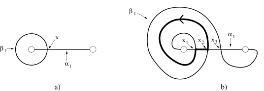
Figure 1. Heegaard splittings of a) $S^{3}$ and b) the lens space $L(3,1)$.

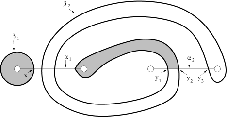
Figure 2. Another splitting of $S^{3}$. The shaded region is the domain of a differential.

2.2. Generators

Let $(\Sigma,\alpha,\beta)$ be a Heegaard splitting of $Y$. The system of attaching circles $\alpha$ defines a Lagrangian torus

$${{\bf T}}_{\alpha}=\{\alpha_{1}\times\alpha_{2}\times\ldots\times\alpha_{g}\}\subset s^{g}\Sigma$$

where $s^{g}\Sigma$ is the $g$th symmetric product of $\Sigma$. The simplest Ozsváth-Szabó  homology, ${{\widehat{HF}}}(Y)$, is a Lagrangian Floer homology defined by the pair $({{\bf T}}_{\alpha},{{\bf T}}_{\beta})$ inside of the symplectic manifold $s^{g}\Sigma$. The generators of the complex ${{\widehat{CF}}}(Y)$ are the points in ${{\bf T}}_{\alpha}\cap{{\bf T}}_{\beta}$. The differential between two generators ${{{\bf y}}}$ and ${{{\bf z}}}$ is defined by counting “holomorphic disks” joining ${{{\bf y}}}$ to ${{{\bf z}}}$; that is, psuedoholomorphic maps $\phi{{\colon}}D^{2}\to s^{g}\Sigma$ such that $\phi(-1)={{{\bf y}}}$, $\phi(1)={{{\bf z}}}$, $\phi(C_{-})\subset{{\bf T}}_{\alpha}$, and $\phi(C_{+})\subset{{\bf T}}_{\beta}$. ($C_{\pm}$ are the components of $\partial D^{2}$ lying above and below the real axis.) We denote the set of homotopy classes of such disks by $\pi_{2}({{{\bf y}}},{{{\bf z}}})$. For $g>1$, this set is either empty or an affine space modeled on $\pi_{2}(s^{g}\Sigma)\cong{\bf{Z}}$. In order to define ${{\widehat{CF}}}$, we must specify which homotopy class we want to count holomorphic disks in, as described in section 2.4 below.

In [19], Ozsváth and Szabó showed that the homology group ${{\widehat{HF}}}(Y)$ has two remarkable properties. First, it does not depend on the choice of Heegaard splitting used for $Y$. Second, all of the objects involved can be described in terms of the Heegaard diagram $(\Sigma,\alpha,\beta)$. For example, the points in ${{\bf T}}_{\alpha}\cap{{\bf T}}_{\beta}$ correspond to unordered $g$-tuples of intersection points $\{x_{1},x_{2},\ldots x_{g}\}$ between the $\alpha_{i}$’s and the $\beta_{j}$’s, such that every $\alpha_{i}$ and $\beta_{j}$ contains exactly one $x_{k}$. Thus if we use the diagram of Figure 1a, we see that ${{\widehat{CF}}}(S^{3})$ is generated by the single intersection point $x$, so ${{\widehat{HF}}}(S^{3})\cong{\bf{Z}}$. If we use the diagram of Figure 2, however, ${{\widehat{CF}}}$ is generated by the three pairs $\{x,y_{1}\},\{x,y_{2}\}$, and $\{x,y_{3}\}$. Since ${{\widehat{HF}}}(S^{3})\cong{\bf{Z}}$, there must be a nontrivial differential in this complex.

2.3. $\epsilon$-grading and basepoints

Given generators ${{{\bf y}}},{{{\bf z}}}\in{{\bf T}}_{\alpha}\cap{{\bf T}}_{\beta}$, there is a topological obstruction to the existance of a disk in $\pi_{2}({{{\bf y}}},{{{\bf z}}})$. As an example, consider the points $x_{1}$ and $x_{2}$ of Figure 1b. The heavy line traces out a curve which goes from $x_{1}$ to $x_{2}$ along ${{\bf T}}_{\alpha}=\alpha_{1}$ and then from $x_{2}$ to $x_{1}$ along ${{\bf T}}_{\beta}=\beta_{1}$. This curve represents a nontrivial class $m$ in the homology of $s^{1}\Sigma=T^{2}$, so it cannot bound a disk. We could try to rectify this problem by choosing different paths from $x_{1}$ to $x_{2}$ along $\alpha_{1}$ and from $x_{2}$ to $x_{1}$ along $\beta_{1}$. This has the effect of replacing the homology class $m$ with $m+a[\alpha_{1}]+b[\beta_{1}]$ for some $a,b\in{\bf{Z}}$. It is easy to see that the resulting homology class is always nonzero, so $\pi_{2}(x_{1},x_{2})$ is empty.

In general, the obstruction can be expressed as a map

$$\epsilon{{\colon}}{{\bf T}}_{\alpha}\cap{{\bf T}}_{\beta}\to\text{Affine}(H_{1}(Y))$$

which we call the $\epsilon$-grading. To define this grading, we use the notion of a system of paths joining ${{{\bf y}}}=\{y_{1},\ldots,y_{g}\}$ to ${{{\bf z}}}=\{z_{1},\ldots,z_{g}\}$ on $\Sigma$. Such a system is a set of polygons with a total of $2g$ edges, which map to $\Sigma$ in the following way: vertices go alternately to $y_{i}$’s and $z_{j}$’s, and edges go alternately to $\alpha_{i}$’s and $\beta_{j}$’s. Every $y_{i}$ and $z_{j}$ is the image of exactly one vertex and every $\alpha_{i}$ and $\beta_{j}$ contains the image of exactly one edge. If $C({{{\bf y}}},{{{\bf z}}})$ is such a system, then $\epsilon({{{\bf y}}})-\epsilon({{{\bf z}}})$ is the image of $C({{{\bf y}}},{{{\bf z}}})$ in

$$\frac{H_{1}(s^{g}\Sigma)}{H_{1}({{\bf T}}_{\alpha})\oplus H_{1}({{\bf T}}_{\beta})}\cong\frac{H_{1}(\Sigma)}{\langle\alpha_{i},\beta_{j}\rangle}\cong H_{1}(Y).$$

The $\epsilon$-grading is always easy to compute. Indeed, as we describe in the next section, it is essentially just a geometric realization of Fox calculus. It divides the points in ${{\bf T}}_{\alpha}\cap{{\bf T}}_{\beta}$ into equivalence classes, which we call $\epsilon$-classes. Two points ${{{\bf y}}},{{{\bf z}}}\in{{{{\bf T}}_{{\alpha}}\cap{{\bf T}}_{{\beta}}}}$ are in the same equivalence class if and only if there is a system of paths $C({{{\bf y}}},{{{\bf z}}})$ which bounds in $\Sigma$. When $b_{1}(Y)=0$, this system is unique.

The set of $\epsilon$-classes is an affine space modeled on $H_{1}(Y)\cong H^{2}(Y)$. The choice of a basepoint $z\in\Sigma-\alpha-\beta$ defines a correspondence between $\epsilon$-classes and ${{\mathrm{Spin}^{c}}}$ structures on $Y$. The ${{\mathrm{Spin}^{c}}}$ structure associated to an $\epsilon$-class $E$ is denoted by ${{\mathbf{s}}}_{z}(E)$. To change the ${{\mathrm{Spin}^{c}}}$ structure we are considering, we can vary either the $\epsilon$-class, the basepoint, or both. This fact is a very useful feature of the Ozsváth-Szabó  Floer homology.

2.4. Domains and differentials

Suppose ${{{\bf y}}}$ and ${{{\bf z}}}$ are two generators in the same $\epsilon$-class, so they are connected by a system of curves $C({{{\bf y}}},{{{\bf z}}})$ which bounds in $\Sigma$. Then the set of 2-chains ${{\mathcal{D}}}$ in $\Sigma$ with $\partial{{\mathcal{D}}}=C({{{\bf y}}},{{{\bf z}}})$ is isomorphic to $H_{2}(\Sigma)\cong{\bf{Z}}$. In fact, Lemma 3.6 of [19] establishes a natural correspondance between such ${{\mathcal{D}}}$’s and the elements of $\pi_{2}({{{\bf y}}},{{{\bf z}}})$. Roughly speaking, the chain ${{\mathcal{D}}}(\phi)$ is the image of a $g$-fold branched cover of $\phi$ induced by the $(g!)$-fold cover $\Sigma^{g}\to s^{g}\Sigma$. (This explains the definition of a system of paths: it is just a $g$-fold cover of $\partial\phi$). We call the chain corresponding to $\phi$ the domain of $\phi$ and denote it by ${{\mathcal{D}}}(\phi)$. Adding a copy of $\Sigma$ to ${{\mathcal{D}}}(\phi)$ corresponds to connect summing $\phi$ with the generator of $\pi_{2}(s^{g}\Sigma)$. (A more detailed treatment of domains is given in the appendix on differentials.)

For $x\in\Sigma-\alpha-\beta$, we denote by $n_{x}(\phi)$ the multiplicity of ${{\mathcal{D}}}(\phi)$ over the component of $\Sigma-\alpha-\beta$ containing $\phi$. If $\phi\in\pi_{2}({{{\bf y}}},{{{\bf z}}})$ has a holomorphic representative, the fact that holomorphic maps are orientation preserving shows that $n_{x}(\phi)\geq 0$ for all $x$. This is a useful tool for showing that a class $\phi$ does not admit any holomorphic representatives.

To each $\phi\in\pi_{2}({{{\bf y}}},{{{\bf z}}})$ we associate the Maslov index $\mu(\phi)$, which is the formal dimension of the space of holomorphic disks in the class $\phi$. The parity of $\mu(\phi)$ is determined by the intersection number: it is even if ${{{\bf y}}}$ and ${{{\bf z}}}$ both have the same sign of intersection, and odd if they do not. In the appendix, we give a combinatorial formula for computing $\mu(\phi)$ from ${{\mathcal{D}}}(\phi)$. It is often useful to know how the Maslov index of different elements of $\pi_{2}({{{\bf y}}},{{{\bf z}}})$ are related: if ${{\mathcal{D}}}(\phi^{\prime})={{\mathcal{D}}}(\phi)+n[\Sigma]$, then $\mu(\phi^{\prime})=\mu(\phi)+2n$.

Fix an $\epsilon$-class $E$ and a basepoint $z$. Then the complex ${{\widehat{CF}}}(Y,{{\mathbf{s}}}_{z}(E))$ is generated by the elements of $E$. The grading and the differentials are defined as follows: for ${{{\bf y}}},{{{\bf z}}}\in E$, let $\phi_{0}({{{\bf y}}},{{{\bf z}}})\in\pi_{2}({{{\bf y}}},{{{\bf z}}})$ be the class with $n_{z}(\phi({{{\bf y}}},{{{\bf z}}}))=0$. Then

$${{\mathrm{gr}}}{{\thinspace}}{{{\bf y}}}-{{\mathrm{gr}}}{{\thinspace}}{{{\bf z}}}=\mu(\phi_{0}({{{\bf y}}},{{{\bf z}}})).$$

If $\mu(\phi_{0}({{{\bf y}}},{{{\bf z}}}))=1$, the moduli space ${\mathcal{M}}(\phi_{0}({{{\bf y}}},{{{\bf z}}}))$ of pseudoholomorphic disks in the class $\phi_{0}({{{\bf y}}},{{{\bf z}}})$ is generically one dimensional and endowed with a free action of ${\bf{R}}$. The ${{{\bf z}}}$ component of $d({{{\bf y}}})$ is defined to be the number of points in the quotient ${{\widehat{\mathcal{M}}}}(\phi_{0}({{{\bf y}}},{{{\bf z}}}))$, counted with sign. (Throughout this section, we gloss over the technical issues of compactness, transversality and orientability for these moduli spaces. These subjects are important, but their treatment in the Ozsváth-Szabó  theory is essentially the same as in Lagrangian Floer homology.)

In certain cases the number of points in ${\widehat{\mathcal{M}}}(\phi)$ depends only on the topology of the domain ${{\mathcal{D}}}(\phi)$. If ${{\mathcal{D}}}$ is a region such that $\#{\widehat{\mathcal{M}}}(\phi)=\pm 1$ for any $\phi$ with ${{\mathcal{D}}}(\phi)={{\mathcal{D}}}$, we say that ${{\mathcal{D}}}$ is the domain of a differential. The shaded region in Figure 2 is an example of such a domain. It defines a differential from $\{x,y_{1}\}$ to $\{x,y_{2}\}$.

2.5. ${{CF^{\infty}}}$, ${{CF^{+}}}$, and ${{CF^{-}}}$

In addition to ${{\widehat{CF}}}$, there are also complexes ${{CF^{+}}}$, ${{CF^{-}}}$ and ${{CF^{\infty}}}$ whose generators are obtained by “stacking” copies of the generators of ${{\widehat{CF}}}$. To be precise, the generators of these complexes are of the form $\{[{{{\bf y}}},n]{{\thinspace}}|{{\thinspace}}{{{\bf y}}}\in{{\bf T}}_{\alpha}\cap{{\bf T}}_{\beta}\}$, where $n\geq 0$ for ${{CF^{+}}}$, $n<0$ for ${{CF^{-}}}$ and $n\in{\bf{Z}}$ for ${{CF^{\infty}}}$.

The differential on ${{CF^{\infty}}}(Y)$ is defined in the following way. If ${{{\bf y}}},{{{\bf z}}}\in{{\bf T}}_{\alpha}\cap{{\bf T}}_{\beta}$ have different signs, we let $\phi_{{{{\bf z}}}}\in\pi_{2}({{{\bf y}}},{{{\bf z}}})$ be the class with $\mu(\phi_{{{\bf z}}})=1$. Then

$$d([{{{\bf y}}},n])=\sum_{{{\bf z}}}\#{\widehat{\mathcal{M}}}(\phi_{{{\bf z}}})\cdot[{{{\bf z}}},n-n_{z}(\phi_{{{\bf z}}})].$$

${{CF^{\infty}}}(Y)$ has the following basic properties:

1. It is an $\text{Affine}({\bf{Z}})$ graded chain complex, with

   $${{\mathrm{gr}}}{{\thinspace}}[{{{\bf y}}},n]-{{\mathrm{gr}}}{{\thinspace}}[{{{\bf z}}},m]=\mu(\phi)-2n_{z}(\phi)+2(n-m).$$

2. It is translation invariant: i.e. the map $u{{\colon}}{{CF^{\infty}}}(Y)\to{{CF^{\infty}}}(Y)$ is an isomorphism. This gives ${{CF^{\infty}}}(Y)$ and ${{CF^{\pm}}}(Y)$ the structure of ${\bf{Z}}[u]$ modules.

3. The group ${{CF^{-}}}(Y)$ is a subcomplex, and ${{CF^{\infty}}}(Y)/{{CF^{-}}}(Y)={{CF^{+}}}(Y)$.

The last item implies that there is a long exact sequence

$$\setcounter{MaxMatrixCols}{11}\begin{CD}@>{}>{}>{{HF^{+}}}(Y)@>{}>{}>{{HF^{-}}}(Y)@>{}>{}>{{HF^{\infty}}}(Y)@>{}>{}>{{HF^{+}}}(Y)@>{}>{}>.\end{CD}$$

If $Y$ is a homology sphere, the group ${{HF^{\infty}}}(Y)$ is always isomorphic to ${\bf{Z}}[u,u^{-1}]$. Using this fact and the long exact sequence, it is easy to compute ${{HF^{+}}}$ from ${{HF^{-}}}$ and vice-versa.

Intuitively, we think of the group ${{\widehat{HF}}}(Y)$ as being the ordinary homology of a space with an $S^{1}$ action, and ${{HF^{+}}}(Y)$ as being its equivariant homology. (See [14] for a very elegant Seiberg-Witten realization of this idea.) It is easy to see that the Gysin sequence and spectral sequence relating ordinary and equivariant homology have analogues which relate ${{\widehat{HF}}}$ to ${{HF^{+}}}$.

2.6. Manifolds with $b_{1}>0$ and twisted coefficients

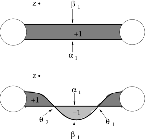
Figure 3. Two Heegaard splittings of $S^{1}\times S^{2}$. The multiplicities of the periodic domains are shown.

For manifolds with $b_{1}>0$, it is no longer true that $\pi_{2}({{{\bf y}}},{{{\bf z}}})\cong{\bf{Z}}$ if ${{{\bf y}}}$ and ${{{\bf z}}}$ are in the same $\epsilon$-class. Instead, $\pi_{2}({{{\bf y}}},{{{\bf z}}})\cong{\bf{Z}}\oplus H_{2}(Y)$. This fact is reflected by the presence of periodic domains: for each class $x\in H_{2}(Y)$, there is a domain ${{\mathcal{P}}}(x)\subset\Sigma$ such that $\partial{{\mathcal{P}}}(x)$ is a sum of the $\alpha_{i}$’s and $\beta_{j}$’s. If $\phi\in\pi_{2}({{{\bf y}}},{{{\bf z}}})$, there is a new disk $\phi+x\in\pi_{2}({{{\bf y}}},{{{\bf z}}})$ with domain ${{\mathcal{D}}}(\phi)+{{\mathcal{P}}}(x)$.

To recover the class $x$ from ${{\mathcal{P}}}(x)$, we put ${{\mathcal{P}}}(x)\subset\Sigma\subset Y$ and “cap off” each of the $\alpha_{i}$’s and $\beta_{j}$’s in $\partial{{\mathcal{P}}}(x)$ with a disk in the appropriate handlebody. This does not uniquely determine ${{\mathcal{P}}}(x)$, since we can always add copies of $\Sigma$ to ${{\mathcal{P}}}(x)$ and get something representing the same homology class. To remedy this problem, we normalize by requiring that $n_{z}({{\mathcal{P}}}(x))=0$.

In order to define the Floer homology of $Y$, we must place some “admissability” conditions on the behavior of the periodic domains. This fact is best illustrated by the two Heegaard splittings for $S^{1}\times S^{2}$ shown in Figure 3. For the first splitting, ${{\bf T}}_{\alpha}\cap{{\bf T}}_{\beta}$ is empty! Since we would like ${{\widehat{HF}}}(S^{1}\times S^{2})$ to be the homology of the circle of reducible Seiberg-Witten solutions, this is not very satisfactory. The solution is to require that all periodic domains have both positive and negative coefficients, as in the second splitting. Now there are two generators $\theta_{1}$ and $\theta_{2}$ and two separate domains which contribute to $d({{{\bf y}}},{{{\bf z}}})$: one positively, and the other negatively. Thus we get a complex which looks exactly like the usual Morse complex for $H_{*}(S^{1})$.

The periodic domains can be used to define twisted versions of the homologies discussed above, with coefficients in $H^{1}(Y)\cong H_{2}(Y)$. To do this, we fix identifications $\Phi:\pi_{2}({{{\bf y}}},{{{\bf z}}})\cong{\bf{Z}}\oplus H_{2}(Y)$ which are consistent, in the sense that if $\phi_{1}\in\pi_{2}({{{\bf y}}},{{{\bf z}}})$ and $\phi_{2}\in\pi_{2}({{{\bf z}}},{\bf w})$, then $\Phi(\phi_{1}+\phi_{2})=\Phi(\phi_{1})+\Phi(\phi_{2})$. Then there is a complex $\underline{{{\widehat{CF}}}}(Y)$ generated by $({{{{\bf T}}_{{\alpha}}\cap{{\bf T}}_{{\beta}}}})\times H_{2}(Y)$ with differential

$$d({{{\bf y}}},a)=\sum_{\{\phi\in\pi_{2}({{{\bf y}}},{{{\bf z}}}){{\thinspace}}|{{\thinspace}}n_{z}(\phi)=0,{{\thinspace}}\mu(\phi)=1\}}\#{\widehat{\mathcal{M}}}(\phi)\cdot({{{\bf z}}},a+\Phi(\phi)).$$

For example, if we use the splitting of Figure 3b, $\underline{{{\widehat{CF}}}}(S^{1}\times S^{2})$ is isomorphic to the complex computing $H_{*}(S^{1})$ with twisted coefficients in $H^{1}(S^{1})$. This is the complex which computes the homology of the universal abelian cover of $S^{1}$, so $\underline{{{\widehat{CF}}}}(S^{1}\times S^{2})\cong{\bf{Z}}$.

The complexes $\underline{{{CF^{\pm}}}}(Y)$ and $\underline{{{CF^{\infty}}}}(Y)$ are defined in an analogous manner.

2.7. Maps and holomorphic triangles

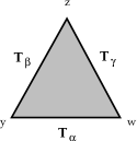
Figure 4. A model triangle.

Maps in the Ozsváth-Szabó  theory are defined by counting holomorphic triangles in Heegaard triple diagrams, which have three sets of attaching handles instead of the usual two. If $(\Sigma,\alpha,\beta,\gamma)$ is such a diagram, it determines a cobordism $W$ from $Y_{1}\coprod Y_{2}$ to $Y_{3}$, where $Y_{1}$ has Heegaard splitting $(\Sigma,\alpha,\beta)$, $Y_{2}$ has splitting $(\Sigma,\beta,\gamma)$, and $Y_{3}$ has splitting $(\Sigma,\alpha,\gamma)$. For each ${{\mathrm{Spin}^{c}}}$ structure ${{\mathbf{s}}}$ on $W$, there is a map

$$\hat{F}_{W,{{\mathbf{s}}}}{{\colon}}{{\widehat{HF}}}(Y_{1})\otimes{{\widehat{HF}}}(Y_{2})\to{{\widehat{HF}}}(Y_{3})$$

defined by counting holomorphic triangles in this diagram.

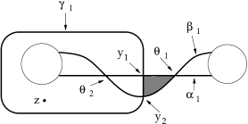
Figure 5. A Heegaard triple diagram for the product cobordism from $S^{3}$ to itself.

More precisely, let $\pi_{2}({{{\bf y}}},{{{\bf z}}},{{{\bf w}}})$ be the set of homotopy classes of maps of the triangle shown in Figure 4 to $s^{g}\Sigma$ which take vertices and edges to the points and tori with which they are labeled. Any $\psi\in\pi_{2}({{{\bf y}}},{{{\bf z}}},{{{\bf w}}})$ determines a ${{\mathrm{Spin}^{c}}}$ structure ${{\mathbf{s}}}_{z}(\psi)$ on $W$ which restricts to the ${{\mathrm{Spin}^{c}}}$ structures ${{\mathbf{s}}}_{z}({{{\bf y}}})$, ${{\mathbf{s}}}_{z}({{{\bf z}}})$, ${{\mathbf{s}}}_{z}({{{\bf w}}})$ on $Y_{1}$, $Y_{2}$, $Y_{3}$ respectively. As in the case of differentials, each triangle $\psi\in\pi_{2}({{{\bf y}}},{{{\bf z}}},{{{\bf w}}})$ has a domain ${{\mathcal{D}}}(\psi)$ which is a 2-chain in $\Sigma$. Triangles which admit holomorphic representatives must have positive domains.

The map $\hat{F}_{W,{{\mathbf{s}}}}$ is induced by a map

$$\hat{f}_{W,{{\mathbf{s}}}}{{\colon}}{{\widehat{CF}}}(Y_{1})\otimes{{\widehat{CF}}}(Y_{2})\to{{\widehat{CF}}}(Y_{3})$$

defined by

$$\hat{f}_{W,{{\mathbf{s}}}}({{{\bf y}}}\otimes{{{\bf z}}})=\sum_{\psi\in A}\#{\widehat{\mathcal{M}}}(\psi)\cdot{{{\bf w}}}$$

where $A=\{\psi\in\pi_{2}({{{\bf y}}},{{{\bf z}}},{{{\bf w}}}){{\thinspace}}|{{\thinspace}}n_{z}(\psi)=\mu(\psi)=0,{{\thinspace}}{{\mathbf{s}}}_{z}(\psi)={{\mathbf{s}}}\}$. There are similarly defined maps on ${{CF^{\pm}}}$ and ${{CF^{\infty}}}$.

In practice, we are usually interested in cobordisms with two boundary components, such as surgery cobordisms. These can be represented by Heegaard triple diagrams for which $Y_{2}=\#^{k}(S^{1}\times S^{2})$. The original cobordism is recovered by “filling in” $Y_{2}$ with $\#^{k}(S^{1}\times D^{3})$. The map $\hat{g}:{{\widehat{CF}}}(Y_{1})\to{{\widehat{CF}}}(Y_{3})$ defined by such a cobordism is given by $\hat{g}({{{\bf y}}})=\hat{f}({{{\bf y}}}\otimes{\bf\theta})$, where ${\bf\theta}$ is the generator of ${{\widehat{HF}}}(\#^{g}(S^{1}\times S^{2}))$ with the highest homological grading. (The reason is that ${\bf\theta}$ is the relative invariant of $\#^{k}(S^{1}\times D^{3})$). This construction can be useful even when the cobordism in question is the product cobordism. In fact, this is how Ozsváth and Szabó prove invariance of their Floer homology under handleslides.

As a simple example, consider the genus one triple diagram shown in Figure 5, which represents the product cobordism from $Y_{1}=S^{3}$ to $Y_{3}=S^{3}$. Thus it induces a map $\hat{f}{{\colon}}{{\widehat{CF}}}(Y_{1})\to{{\widehat{CF}}}(Y_{3})$. ${{\widehat{CF}}}(Y_{1})$ is generated by $y_{1}$, while ${{\widehat{CF}}}(Y_{3})$ is generated by $y_{2}$. ${{\widehat{HF}}}(S^{1}\times S^{2})$ is generated by $\theta_{1}$ and $\theta_{2}$, where $\theta_{1}$ has the higher absolute grading. (We can tell this because the differentials go from $\theta_{1}$ to $\theta_{2}$.) Thus $\hat{f}({{{\bf y}}})$ is defined by counting triangles in $\pi_{2}(y_{1},\theta_{1},y_{2})$. There is a unique such triangle; its domain is shaded in the figure. Using the Riemann mapping theorem, it is easy to see that this triangle has a unique holomorphic representative. Thus $\hat{f}$ is an isomorphism (as it should be). Most of the holomorphic triangles we need to count will have domains that look like this one or the union of several disjoint copies of it.

3. Heegaard splittings and the Alexander grading

This section contains background material on Heegaard splittings for knot complements, the $\epsilon$-grading, and its relation to Fox calculus and the Alexander polynomial. We first consider large $n$-surgery on knots in $S^{3}$ and then generalize to knots in arbitrary three-manifolds. Much of this material may be found in [19] and [18], although we believe the emphasis on Fox calculus is new.

3.1. Heegaard splittings and $\pi_{1}$

Let $Y$ be a three-manifold. To any Heegaard splitting of $Y$ there is naturally associated a presentation of $\pi_{1}(Y)$. To see this, note that $\pi_{1}$ of the handlebody obtained by attaching two-handles along the $\alpha$’s is a free group with $g$ generators, and each two-handle $\beta_{i}$ gives a relator. More specifically, we choose as generators of $\pi_{1}(Y)$ a set of loops $x_{1},x_{2},\ldots,x_{g}$ on $\Sigma$, where $x_{i}$ intersects $\alpha_{i}$ once with intersection number $+1$ and misses all the other $\alpha_{j}$. Then the relator corresponding to $\beta_{i}$ may be found by traversing $\beta_{i}$ and recording its successive intersections with the $\alpha_{j}$’s. Each time $\beta_{i}$ intersects $\alpha_{j}$, we append $x_{j}^{\pm 1}$ to the relator, where $\pm 1$ is the sign of the intersection. There a natural correspondence between allowable moves on a Heegaard splitting and Tietze moves on the associated presentation. Indeed, removing a pair of intersection points by isotopy corresponds to cancelling consecutive appearances of $x_{i}$ and $x^{-1}_{i}$ in some word, stabilization corresponds to adding a new generator and relator, sliding the handle $\alpha_{i}$ over $\alpha_{j}$ corresponds to making the substitution $x_{i}^{\prime}=x_{j}x_{i}x_{j}^{-1}$, and sliding $\beta_{i}$ over $\beta_{j}$ corresponds to conjugating $w_{j}$ by $w_{j}$.

Three-manifolds with boundary also have Heegaard splittings, but with fewer $\beta$ circles than $\alpha$ circles. For example, if $\partial N=T^{2}$, $N$ has a Heegaard splitting with one more $\alpha$ circle than $\beta$ circles. To do Dehn filling on such a manifold, we attach a final two-handle along some curve $\beta_{g}$ disjoint from $\beta_{1},\beta_{2},\ldots\beta_{g-1}$. This gives a Heegaard splitting of the resulting closed manifold.

It is clear that the correspondence between Heegaard splittings and presentations of $\pi_{1}$ holds for the case of manifolds with boundary as well.

3.2. Heegaard splittings of knot complements

Let $K$ be a knot in $S^{3}$. We denote by ${{K^{o}}}$ the manifold obtained by removing a regular neighborhood of $K$ from $S^{3}$. In the next two subsections, we describe this special case in some detail, both to provide background for later sections and to motivate our treatment of a general three-manifold with torus boundary. First, we discuss Heegaard splittings of ${{K^{o}}}$ and how to find them.

We can use a bridge presentation of a knot to find a Heegaard splitting of its exterior. Recall that $K$ is said to be a $g$-bridge knot if it has an embedding in ${\bf{R}}^{3}$ whose $z$ coordinate has $g$ maxima. Any such knot admits a bridge presentation with $g$ bridges, i.e. a planar diagram composed of $2g$ segments $a_{1},a_{2},\ldots a_{g},b_{1},b_{2},\ldots,b_{g}$ such that: i) all of the $a_{i}$’s and all of the $b_{i}$’s are disjoint, and ii) the $b_{i}$’s always overcross the $a_{i}$’s. Given such a presentation of $K$, we can obtain a genus $g$ Heegaard splitting for ${{K^{o}}}$ as follows: let $\Sigma$ be the surface obtained by joining the two endpoints of each $a_{i}$ by a tube, and let $\alpha_{i}$ be a circle which first traverses $a_{i}$ and then goes over the new tube and back to its starting point. Finally, let $\beta_{i}$ be the boundary of a regular neighborhood of $b_{i}$ in the original diagram. The $\beta_{i}$’s are linearly dependent; indeed it is easy to see that $b_{1}+b_{2}+\ldots+b_{g}=0$ in $H_{1}(\Sigma)$. As a consequence, the three-manifold obtained by attaching two-handles along any $g-1$ of the $\beta_{i}$’s is the same as the one obtained by attaching two-handles along all $g$ of them. By convention, we choose to omit $\beta_{g}$, although we could just as well have skipped any of the others.

To see why this construction works, consider the plane of the bridge diagram, which separates $S^{3}$ into two balls. We push the underbridges a little below the plane while leaving the overbridges in it. The intersection of ${{K^{o}}}$ with the lower ball is obtained by removing tubular neighborhoods of the underbridges from the ball. This space is homeomorphic to a handlebody with boundary $\Sigma$ and attaching handles $\alpha_{i}$. To get ${{K^{o}}}$, we glue in two-handles along the $\beta_{i}$ (leaving little tubes around each overbridge), and then fill in the $S^{2}$ boundary component with a ball.

An example of such a Heegaard splitting is shown in Figure 6. In drawing these pictures, we adopt the convention of Section 8 of [19] and show only the part of $\Sigma$ which lies in the plane of the diagram. We do not care much about the orientation of the $\beta_{i}$’s, but we always orient the $\alpha_{i}$’s consistantly, so that $\beta_{i}\cdot(\alpha_{1}+\alpha_{2}+\ldots+\alpha_{g})=0$ for each $i$.

Figure 6. A Heegaard splitting for the exterior of the right-handed $(3,4)$ torus knot. The small circles indicate where the tubes are attached and also represent the $x_{i}$’s.

When our Heegaard splitting comes from a bridge decomposition, the associated presentation of $\pi_{1}$ is just the Wirtinger presentation. In particular, all the relators are of the form $x_{i}wx_{j}^{-1}w^{-1}$ for some word $w$. (Our convention for orienting the $\alpha_{i}$ ensures that $x_{i}$ and $x_{j}$ have opposite exponents.) Abelianizing, we see that the $x_{i}$ are all homologous to other and generate $H_{1}({{K^{o}}})\cong{\bf{Z}}$. In fact, it is immediate from our construction of the Heegaard splitting that the $x_{i}$’s are all meridians of $K$.

Given a curve $\gamma$ in $\Sigma$, we often want to compute its homology class in $H_{1}({{K^{o}}})$. If we let $\alpha=\alpha_{1}+\alpha_{2}+\ldots+\alpha_{g}\in H_{1}(\Sigma)$, it is easy to see that $[\gamma]=(\gamma\cdot\alpha)m$. For example, if we want to find a longitude of $K$ in $\Sigma$, we can start with the curve $\lambda$ obtained by connecting the $b_{i}$’s to each other by arcs going over the handles. We clearly have $m\cdot\lambda=1$, and $\ell=\lambda-(\lambda\cdot\alpha)m$ is null-homologous in ${{K^{o}}}$, so it must be a longitude.

Any planar diagram of $K$ gives a bridge decomposition, but some such decompositions are more suitable for our purposes than others. In general, the smaller the bridge number of our presentation of $K$, the simpler the complex ${{\widehat{CF}}}(K_{n})$ will be. It is thus in our interest to be able to find diagrams of a knot with minimal bridge number. (An exception to this rule may be found in section 8, when we discuss alternating knots.) For two-bridge knots, this problem was solved by Schubert in [27]. Unfortunately, there is no such nice description of $n$-bridge knots, even for $n=3$.

Starting from a diagram of $K$ with $n$ obvious maxima and minima, there is a straightforward algorithm to find a bridge decomposition by successively “unbraiding” $K$. (It is a good exercise to derive the splitting of Figure 6 using this method.) In practice, however, this method requires a lot of patience and chalk. It is usually much easier to use the converse, which implies that every Heegaard splitting of the form described above is a splitting of some knot complement. Given a knot $K$, we write down the Wirtinger presentation for $\pi_{1}({{K^{o}}})$ and use a computer algebra system to simplify the presentation, eliminating generators while keeping the relators in the form $x_{i}wx_{j}^{-1}w^{-1}$. Once we have reduced the presentation to as few generators as possible, we can just try to draw a Heegaard splitting which gives the simplified presentation. A priori, of course, we only know that we have drawn a knot complement with the same $\pi_{1}$ as our original knot. But under very mild hypotheses (such as $K$ being hyperbolic), this is enough to ensure that the knot complement we have drawn corresponds either to $K$ or its mirror image.

3.3. The Alexander grading for knots

We now study the effect of doing $n$ surgery on ${{K^{o}}}$ to get the closed manifold $K(n,1)$. The final attaching circle $\beta_{g}$ will be a curve in $\Sigma-\beta_{1}-\beta_{2}-\ldots-\beta_{g-1}$ homologous to $nm+l$. There are many such curves; we choose the one obtained by taking the union of $\ell$ and $n$ parallel copies of $x_{g}$ and smoothing the intersections to get a simple closed curve $\beta_{g}$. This procedure was introduced in section 8 of [19]; we refer to it as twisting up around $\alpha_{g}$. Of course, our choice of $x_{g}$ was arbitrary — we could just as well have twisted up around any of the other $\alpha_{i}$.

Figure 7. The spiral region of $\beta_{g}$. Note that the handedness of the spiral is determined by the fact that we are doing $+n$ surgery (and the convention that $m\cdot\lambda=+1$.)

Although $\beta_{g}$ can be complicated, the only part of it which will be relevant to us is the spiral region containing the $n$ parallel copies of the meridian, which is illustrated in Figure 7. We label the intersections between $\alpha_{g}$ and $\beta_{g}$ by $w_{i}$. To do this, we must specify the direction of increasing $i$, or equivalently, an orientation of $\ell$. To this end, we fix once and for all a generator of $H_{1}(K(0,1))$. Given a Heegaard splitting of ${{K^{o}}}$, this choice determines an orientation on $m$, and thus on $\ell$.

Our first class is to understand the $\epsilon$-grading associated to this Heegaard diagram. The following observation is trivial, but quite important.

Lemma 3.1.

For $n$ sufficiently large, there is an $\epsilon$-class all of whose elements contain some $w_{i}$.

Proof.

The number of $\epsilon$-classes is $n$, but the number of intersection points ${\bf y}$ which do not contain any $w_{i}$ is bounded independent of $n$. ∎

We will always work with such an $\epsilon$-class. Thus we need only consider elements of ${{{{\bf T}}_{{\alpha}}\cap{{\bf T}}_{{\beta}}}}$ which have the form ${\bf y}=\{\hat{\bf y},w_{i}\}$, where $\hat{\bf y}$ is an intersection point of the tori ${{\bf T}}_{\hat{\alpha}}$ and ${{\bf T}}_{\hat{\beta}}$ defined by the $(g-1)$-fold symmetric products of $\alpha_{1},\alpha_{2},\ldots,\alpha_{g-1}$ and $\beta_{1},\beta_{2},\ldots,\beta_{g-1}$ in $s^{g-1}\Sigma$.

When $n$ is large, most $\epsilon$-classes contains precisely one point of the form $\{\hat{\bf y},w_{i}\}$ for each ${{\hat{{\bf y}}}}\in{{{{\bf T}}_{\hat{\alpha}}\cap{{\bf T}}_{\hat{\beta}}}}$. Indeed, it is easy to see from Figure 7 that

$$\epsilon(\{{{\hat{{\bf y}}}},w_{i}\})-\epsilon(\{{{\hat{{\bf y}}}},w_{j}\})=(j-i)[m],$$

so a given $\epsilon$-class can contain no more than one such point. On the other hand

$$\epsilon(\{{{\hat{{\bf y}}}},w_{i}\})-\epsilon(\{{{\hat{{\bf z}}}},w_{i}\})=k[m],$$

for some $k$, since $[m]$ generates $H_{1}(K_{n})$. Then by the additivity of $\epsilon$,

$$\epsilon(\{{{\hat{{\bf y}}}},w_{i}\})-\epsilon(\{{{\hat{{\bf z}}}},w_{i-k}\})=k[m]-k[m]=0,$$

so $\{{{\hat{{\bf y}}}},w_{i}\}$ and $\{{{\hat{{\bf z}}}},w_{i-k}\}$ are in the same $\epsilon$-class. (Our labeling is modulo $n$, so that if $i-k\leq 0$, we interpret $w_{i-k}$ as $w_{i-k+n}$.)

Now it is easy to see that if $\{\hat{\bf y},w_{A({{\hat{{\bf y}}}})}\}$ are the points in one $\epsilon$-class, $\{\hat{\bf y},w_{A({{\hat{{\bf y}}}})+k}\}$ will be the points in another. Thus most $\epsilon$-classes look very similar — they are just translates of each other. When the values of $A({{\hat{{\bf y}}}})+k$ get close to $1$ or $n$, there will be some “wrapping” from one side of the spiral to another, but when $n$ is large, most $\epsilon$-classes will have values of $A({{\hat{{\bf y}}}})+k$ far away from $1$ and $n$. To summarize, we have the following

Proposition 3.1.

There is a number $M$ independent of $n$ so that all but $M$ $\epsilon$-classes are of the form $\{\{{{\hat{{\bf y}}}},w_{k+A({{\hat{{\bf y}}}})}\}{{\thinspace}}|{{\thinspace}}{{\hat{{\bf y}}}}\in T_{\hat{\alpha}}\cap T_{\hat{\beta}}\}$ for some value of $k$.

The function $A$ is most naturally thought of as an affine-valued grading

$$A:T_{\hat{\alpha}}\cap T_{\hat{\beta}}\to\text{\it Affine}({\bf{Z}}),$$

which we refer to as the Alexander grading. Our choice of name is explained by

Proposition 3.2.

Let ${{{\text{sign}}}}({{\hat{{\bf y}}}})$ denote the sign of the intersection between $T_{\hat{\alpha}}$ and $T_{\hat{\beta}}$ at ${{\hat{{\bf y}}}}$. Then

$$\sum_{{{\hat{{\bf y}}}}\in{{{{\bf T}}_{\hat{\alpha}}\cap{{\bf T}}_{\hat{\beta}}}}}{\text{s}ign}({{\hat{{\bf y}}}})\ t^{A({{\hat{{\bf y}}}})}$$

represents the Alexander polynomial $\Delta_{K}(t)$ of $K$.

Remark: The Alexander polynomial is defined only up to a factor of $\pm t^{k}$, reflecting the fact that $A$ is only an affine grading. The symmetry of $\Delta_{K}(t)$ gives us a natural choice of representative, however, namely the one for which $\Delta_{K}(t)=\Delta_{K}(t^{-1})$ and $\Delta_{K}(1)=1$. We will always assume $\Delta_{K}(t)$ satisfies these properties. To indicate the weaker condition $P(t)=\pm t^{k}\Delta_{K}(t)$, we write “$P(t)$ represents $\Delta_{K}(t)$,” or simply $P(t)\sim\Delta_{K}(t)$.

Our choice of a distinguished representative for the Alexander polynomial gives us a natural lift of $A$ to a ${\bf{Z}}$ valued map; namely the one for which the sum above is actually equal to $\Delta_{K}(t)$. From now on we use this lift, which we continue to denote by $A$.

Proposition 3.2 is a corollary of the following principle, which is very helpful in making computations:

Principle 3.1.

The process of computing the elements of ${{{{\bf T}}_{\hat{\alpha}}\cap{{\bf T}}_{\hat{\beta}}}}$ and their Alexander gradings is identical to the process of computing the Alexander polynomial of $K$ by Fox calculus.

More precisely, our choice of Heegaard splitting naturally gives us a presentation $P=\langle x_{1},x_{2},\ldots,x_{g}{{\thinspace}}|{{\thinspace}}w_{1},w_{2},\ldots,w_{g-1}\rangle$ of $\pi_{1}({{K^{o}}})$. Recall from [2] that to compute the Alexander polynomial of $K$ from $P$, we take the determinant

$$(d_{x_{i}}w_{j})_{1\leq i,j\leq g-1}.$$

of the matrix of free differentials. If we take the free differentials, expand the determinant, and multiply out without ever combining terms, the monomials of the resulting Laurent polynomial will naturally correspond to the points of ${{{{\bf T}}_{\hat{\alpha}}\cap{{\bf T}}_{\hat{\beta}}}}$, with their exponents giving the Alexander grading and their signs giving the sign of intersection.

3.4. Fox Calculus and Closed Manifolds

We now extend the ideas of the preceding section to more general three-manifolds. First, we describe the relationship between Fox calculus and the $\epsilon$-grading on a closed manifold $Y$. We choose a Heegaard splitting $(\Sigma,{{\mathbf{\alpha}}},{{\mathbf{\beta}}})$ of $Y$ and take $P$ to be the associated presentation of $\pi_{1}(Y)$.

Principle 3.2.

The process of computing the points of ${{\bf T}}_{\alpha}\cap{{\bf T}}_{\beta}$ and their $\epsilon$-gradings is identical to the process of computing the $0$-th Alexander ideal associated to the presentation $P$.

Actually, we need to use a slight variation of the usual version of Fox calculus: we take coefficients in the group ring ${\bf{Z}}[H_{1}(Y)]$ rather than in ${\bf{Z}}[H_{1}(Y)/{\text{\it Torsion}}]$. (The first ring is usually used because one needs a UFD to define the greatest common divisor. Since we will never take $\gcd$’s, there is no problem with using the larger ring.)

The first step in establishing the principle is to observe that the $\epsilon$-grading satifies a slightly stronger version of additivity.

Lemma 3.2.

For points ${\bf y}=\{y_{1},y_{2},\ldots,y_{g}\}$ and ${\bf y}^{\prime}=\{y_{1}^{\prime},y_{2},\ldots,y_{g}\}$ in ${{{{\bf T}}_{{\alpha}}\cap{{\bf T}}_{{\beta}}}}$, the difference $\epsilon(\{y_{1},y_{2},\ldots,y_{g}\})-\epsilon(\{y_{1}^{\prime},y_{2},\ldots,y_{g}\})$ depends only on $y_{1}$ and $y_{1}^{\prime}$.

Proof.

Suppose $y_{1}$ is an intersection point of $\alpha_{i}$ and $\beta_{j}$. Then $y_{1}^{\prime}$ is another intersection point of $\alpha_{i}$ and $\beta_{j}$, since these are the only curves which do not contain one of $y_{2},\ldots,y_{g}$. To compute $\epsilon(\{y_{1},y_{2},\ldots,y_{g}\})-\epsilon(\{y_{1}^{\prime},y_{2},\ldots,y_{g}\})$, we consider the system of loops in $\Sigma$ obtained by going from $y_{1}$ to $y_{1}^{\prime}$ along $\alpha_{i}$ and from $y_{1}^{\prime}$ to $y_{1}$ along $\beta_{j}$, and then joining each $y_{i}$, $i\geq 2$ to itself by the trivial loop. The homology class of this system is just the class of the first loop, which depends only on $y_{1}$ and $y_{1}^{\prime}$. ∎

Thus for each $i$ and $j$ we have a well-defined affine grading

$$\epsilon_{ij}:\alpha_{i}\cap\beta_{j}\to{\text{\it Affine}}(H_{1}(N))$$

given by the homology class of this loop. Repeated application of the lemma shows that if $\{y_{1},y_{2},\ldots y_{g}\}$ and $\{y_{1}^{\prime},y_{2}^{\prime},\ldots y_{g}^{\prime}\}$ share the same combinatorics, i.e. $y_{k}$ and $y_{k}^{\prime}$ are both intersection points of the same $\alpha_{i_{k}}$ and $\beta_{j_{k}}$, then

$$A(\{y_{1},y_{2},\ldots,y_{g}\})-A(\{y_{1}^{\prime},y_{2}^{\prime},\ldots,y_{g}^{\prime}\})=\sum_{k=1}^{g}\epsilon_{i_{k}j_{k}}(y_{k})-\epsilon_{i_{k}j_{k}}(y_{k}^{\prime})$$

We now relate $\epsilon_{ij}$ to the free differential.

Lemma 3.3.

$$d_{x_{i}}w_{j}\sim\sum_{y\in\alpha_{i}\cap\beta_{j}}\text{sign}(y)\ {\epsilon_{ij}(y)}$$

Proof.

Each intersection $y\in\alpha_{i}\cap\beta_{j}$ corresponds to an appearance of $x_{i}^{\text{sign}(y)}$ in $w_{j}$, and thus to a monomial ${{\text{sign}}}(y)f(y)$ in $d_{x_{i}}w_{j}$. We claim that $f(y)\sim\epsilon_{ij}(y)$. Indeed, suppose that $y_{1}$ and $y_{2}$ are two elements of $\alpha_{i}\cap\beta_{j}$. Assume first that both intersections are positive, so that $w_{j}$ has a segment of the form $x_{i}x^{a_{1}}_{i_{1}}x^{a_{2}}_{i_{2}}\cdots x^{a_{n}}_{i_{n}}x_{i}$, where the two appearances of $x_{i}$ correspond to $y_{1}$ and $y_{2}$ respectively. Then $f(y_{2})-f(y_{1})$ is the image of $x_{i}x^{a_{1}}_{i_{1}}x^{a_{2}}_{i_{2}}\cdots x^{a_{n}}_{i_{n}}$ in $H_{1}(N)$. On the other hand, $\epsilon_{ij}(y_{2})-\epsilon_{ij}(y_{1})$ is the homology class of the loop which starts just after the first $y_{1}$, travels along $\beta_{j}$ until just before the second $y_{2}$, and then returns to its starting point along $\alpha_{i}$, going up once through $\alpha_{i}$ in the process. Thus this loop is also represented by $x_{i}x^{a_{1}}_{i_{1}}x^{a_{2}}_{i_{2}}\cdots x^{a_{n}}_{i_{n}}$. This proves the lemma when both intersections are positive. The other cases are similar. ∎

The $0$-th Alexander ideal is generated by the determinant of the matrix of free differentials:

$$(d_{x_{i}}w_{j})_{1\leq i,j\leq g}.$$

Proposition 3.3.

$$\det(d_{x_{i}}w_{j})\sim\sum_{{\bf y}\in{{{{\bf T}}_{{\alpha}}\cap{{\bf T}}_{{\beta}}}}}{\text{s}ign}\ ({\bf y})\ {\epsilon({\bf y})}$$

Proof.

We expand the determinant as a sum

$$\sum_{\sigma\in S_{g}}{{\text{sign}}}(\sigma)\ d_{1}w_{\sigma(1)}d_{2}w_{\sigma(2)}\cdots d_{g}w_{\sigma(g)}$$

and multiply out without ever combining terms. We claim that the monomials in the resulting polynomial correspond precisely to the points of ${{{{\bf T}}_{{\alpha}}\cap{{\bf T}}_{{\beta}}}}$. Indeed, to specify a point of ${{{{\bf T}}_{{\alpha}}\cap{{\bf T}}_{{\beta}}}}$, we must first choose a partition of the $\alpha_{i}$’s and $\beta_{j}$’s into $g$ sets, each containing one $\alpha_{i}$ and one $\beta_{j}$, which corresponds to picking a permutation $\sigma\in S_{g}$. Then for each pair $\{\alpha_{i},\beta_{\sigma(i)}\}$ we must choose a point in $\alpha_{i}\cap\beta_{\sigma(i)}$. This corresponds to picking a monomial out of each term $d_{x_{i}}w_{\sigma(i)}$ appearing in the product, or equivalently, a single monomial from the expanded product. Thus each ${{{\bf y}}}\in{{{{\bf T}}_{{\alpha}}\cap{{\bf T}}_{{\beta}}}}$ is associated to some monomial $\pm f({{{\bf y}}})$ in the expansion of the determinant.

We claim that for ${{{\bf y}}},{{{\bf z}}}\in{{{{\bf T}}_{{\alpha}}\cap{{\bf T}}_{{\beta}}}}$, $f({{{\bf y}}})-f({{{\bf z}}})=\epsilon({{{\bf y}}})-\epsilon({{{\bf z}}})$. Lemmas 3.2 and 3.3 show that this is true for intersection points ${{\hat{{\bf y}}}}$ and ${{\hat{{\bf z}}}}$ which have the same combinatorics. To check it in general, we consider the loop representing $\epsilon(\{y_{1},y_{2},y_{3},\ldots,y_{g}\})-\epsilon(\{y_{1}^{\prime},y_{2}^{\prime},y_{3},\ldots,y_{g}\})$ and argue, as in the proof of Lemma 3.3, that this loop also represents the difference appearing in the free differential. This proves the claim when $g-2$ of the points in ${\bf y}$ and ${\bf y}^{\prime}$ are the same, and the general result follows by repeated application of this fact. (If necessary, we introduce some extra pairs of intersection points to ensure that each product in the determinant is nonempty.)

Finally, we check that the sign of the monomial associated to ${{{\bf y}}}$ is the sign of the intersection. Locally, each ${\bf y}\in{{{{\bf T}}_{{\alpha}}\cap{{\bf T}}_{{\beta}}}}$ looks like a product of intersections $\alpha_{i}\cap\beta_{\sigma(i)}$ in $\Sigma$. Now

$$(\alpha_{1}\times\alpha_{2}\times\ldots\times\alpha_{g})\cdot(\beta_{\sigma(1)}\times\beta_{\sigma(2)}\times\ldots\times\beta_{\sigma(g)})=(\alpha_{1}\cdot\beta_{\sigma(1)})(\alpha_{2}\cdot\beta_{\sigma(2)})\cdots(\alpha_{g}\cdot\beta_{\sigma(g)})$$

is the sign of the monomial corresponding to ${{{\bf y}}}$ in $d_{1}w_{\sigma(1)}d_{2}w_{\sigma(2)}\cdots d_{g}w_{\sigma(g)}$. Since the product orientation on $(\beta_{\sigma(1)}\times\beta_{\sigma(2)}\times\ldots\times\beta_{\sigma(g)})$ is ${{\text{sign}}}(\sigma)$ times the usual orientation, the signs are correct. ∎

Thus we have verified Principle 3.2. An analogue of Proposition 3.2 holds as well, but is rather uninteresting, since it amounts to the well-known fact that $\chi({{\widehat{CF}}}(N))$ is $1$ if $b_{1}(N)=0$ and $0$ otherwise.

3.5. The Alexander grading in general

We now describe the analogues of Propositions 3.1 and 3.2 for a knot in a general three-manifold. We prefer to think about the knot complement $N$, which is a manifold with torus boundary. Any three-manifold with torus boundary has a class $l\in H_{1}(\partial N)$ which bounds in $N$; if $N$ is a knot complement, $l$ may be chosen to be primitive in $H_{1}(\partial_{N})$. There are two possible choices of such an $l$ — we fix one of them. Next, we choose a class $m\in H_{1}(\partial N)$ with $m\cdot l=1$ to play the role of the meridian. Unlike the choice of $l$, which is just a sign convention, this choice of $m$ is very important. Everything that follows will depend on which $m$ we pick. We write $N(p,q)$ for the closed manifold obtained by doing Dehn filling on $pm+ql$. We will often need to consider $N(1,0)$, which we denote by ${{\overline{N}}}$.

We now proceed much as we did for knots in $S^{3}$. We choose a Heegaard splitting $(\Sigma,{{\mathbf{\alpha}}},{{\mathbf{\beta}}})$ of $N$ and represent $m$ and $l$ by curves ${{\mathfrak{m}}}$ and $\ell$ on $\Sigma$ disjoint from the $\beta$’s. The most significant difference from the knot case is that ${{\mathfrak{m}}}$ may have many intersections with the $\alpha_{i}$’s, rather than a single one. If we wish, however, we can always reduce to the latter case by increasing the genus of our Heegaard splitting.

Lemma 3.4.

Any Heegaard splitting of $N$ is equivalent to one in which ${{\mathfrak{m}}}$ intersects a single $\alpha_{i}$ geometrically once.

Proof.

Stabilize the Heegard splitting by connect summing $\Sigma$ with the genus 1 Heegaard splitting for $S^{3}$. Call the new attaching handles $\alpha_{g+1}$ and $\beta_{g}$. Then we can slide $m$ over $\beta_{g}$ so it has a single intersection with $\alpha_{g+1}$. Now remove the intersections of $m$ with the other $\alpha_{i}$ by sliding them over $\alpha_{g+1}$. ∎

Despite this fact, we will continue to work in the more general setting, since it is needed for the proof of Theorem 1.

Figure 8. The spiral region for a general Heegaard splitting

To get a Heegaard splitting of $N(n,1)$, we let $\beta_{g}$ be the curve obtained by taking the union of $\ell$ with $n$ parallel copies of ${{\mathfrak{m}}}$ and then resolving. As in the knot case, we take $n\gg 0$ and focus on the spiral region shown in Figure 8. We label the segments of the $\alpha$ curves passing through the spiral $w^{1},w^{2},\ldots,w^{m}$. We will need to know which $\alpha_{j}$ contains $w_{i}$, so we fix numbers $m_{i}$ so that $w^{i}\subset\alpha_{m_{i}}$. Finally, we label the individual intersection points on by $w^{i}_{j}$, using our chosen orientation on $l$ to determine the direction of increasing $i$.

When $n$ is large, most points in ${{\bf T}}_{\alpha}\cap{{\bf T}}_{\beta}$ will be of the form ${{{\bf y}}}=\{{{\hat{{\bf y}}}},w^{i}_{j}\}$ for ${{\hat{{\bf y}}}}\in{{\bf T}}_{\widehat{\alpha_{m_{i}}}}\cap{{\bf T}}_{\hat{\beta}}$, where $T_{\widehat{\alpha_{m_{i}}}}$ is the torus in $s^{g-1}\Sigma$ determined by the symmetric product of $\alpha_{1},\alpha_{2},\ldots,\hat{\alpha_{i}},\ldots\alpha_{g}$. We often think of the point ${{{\bf y}}}$ as lying over $w^{i}_{j}$, and write $w({{{\bf y}}})=w^{i}_{j}$.

To each ${{{\bf y}}}=\{{{\hat{{\bf y}}}},w^{i}_{j}\}$, there is an associated point $\overline{{{{\bf y}}}}=\{{{\hat{{\bf y}}}},w^{i}\}$ in ${{\bf T}}_{\alpha}\cap{{\bf T}}_{{{\overline{{{\mathbf{\beta}}}}}}}$, where $(\Sigma,{{\mathbf{\alpha}}},{{\overline{{{\mathbf{\beta}}}}}})$ is the Heegaard splitting for ${{\overline{N}}}$ obtained by taking ${{\overline{\beta}}}_{g}=m$. We let ${{\overline{\epsilon}}}$ denote the $\epsilon$-grading on the $\{{{\hat{{\bf y}}}},w^{i}\}$ associated to this Heegaard splitting. It is easy to see that ${{\overline{\epsilon}}}(\overline{{{{\bf y}}}})$ is the image of $\epsilon({{{\bf y}}})$ under the projection

$$H_{1}(N)/n\langle m\rangle\to H_{1}(N)/\langle m\rangle\cong H_{1}({{\overline{N}}}).$$

There are ${\bf{Z}}/n$ $\epsilon$-classes over each ${{\overline{\epsilon}}}$-class, and if $\{{{\hat{{\bf y}}}},w^{i}\}$ is in an ${{\overline{\epsilon}}}$-class, one of the $\{{{\hat{{\bf y}}}},w^{i}_{j}\}$ is in each of the $\epsilon$-classes above it.

Proposition 3.4.

There is an number $M$ independent of $n$ such that for any ${{\overline{\epsilon}}}$-class ${{\overline{E}}}$, all but $M$ of the $\epsilon$-classes above ${{\overline{E}}}$ are of the form

$$\{\{{{\hat{{\bf y}}}},w^{i}_{k+A({{\hat{{\bf y}}}},w^{i})}\}{{\thinspace}}|{{\thinspace}}\{{{\hat{{\bf y}}}},w^{i}\}\in{{\overline{E}}}\}$$

Proof.

The number of points in ${{{{\bf T}}_{{\alpha}}\cap{{\bf T}}_{{\beta}}}}$ not of the form $\{{{\hat{{\bf y}}}},w^{i}_{k+A({{\hat{{\bf y}}}},w^{i})}\}$ is bounded independent of $n$. The number of $\epsilon$-classes above ${{\overline{E}}}$ in which the points “wrap” (so that some of them are on the left end of the spiral while others are on the right) is also bounded independent of $n$. Finally, $\epsilon(\{{{\hat{{\bf y}}}},w^{i}_{j})-\epsilon(\{{{\hat{{\bf y}}}},w^{i}_{l}\})=(l-j)m$, so if $\{{{\hat{{\bf y}}}},w^{i}_{A({{\hat{{\bf y}}}},w^{i})}\}$ are all in one $\epsilon$-class, so are $\{{{\hat{{\bf y}}}},w^{i}_{A({{\hat{{\bf y}}}},w^{i})}\}$. ∎

We call a class of this form as a good $\epsilon$-class. The map $A:{{\overline{E}}}\ \to{\text{\it Affine}}({\bf{Z}})$ is the Alexander grading. The sign of the Alexander grading depends on our choice of orientation for $l$ — reversing the orientation gives the opposite sign. (This reflects the fact that our representation of the Alexander polynomial depends on a choice of basis for $H_{1}$.) To summarize, we have

Corollary 3.1.

Any two points in a good $\epsilon$-class are joined by null-homologous system of paths whose $\beta_{g}$ component is supported inside the spiral region. The difference in their Alexander gradings is just the number of times the $\beta_{g}$ component intersects the dashed line in Figure 8.

Proof.

The corresponding points in $T_{\alpha}\cap T_{{{\overline{\beta}}}}$ are in the same ${{\overline{\epsilon}}}$-class, so they can be joined by a null-homologous system of paths along $\alpha_{1},\alpha_{2},\ldots,\alpha_{g},\beta_{1},\beta_{2},\ldots,\beta_{g-1},{{\mathfrak{m}}}$. The path for the original points is the same, but with the ${{\mathfrak{m}}}$ component lifted up to the spiral region. ∎

Proposition 3.5.

The process of finding the ${{\overline{\epsilon}}}$-classes and Alexander gradings of all the points $\{{{\hat{{\bf y}}}},w^{i}\}$ is the same as that of computing

$$\det(d_{i}w_{j})_{1\leq i,j\leq g}$$

with coefficients in ${\bf{Z}}[H_{1}(N)]$.

Proof.

If we reduce coefficients to ${\bf{Z}}[H_{1}({{\overline{N}}})]$, Principle 3.2 shows that the determinant computes the ${{\overline{\epsilon}}}$-gradings of the $\{{{\hat{{\bf y}}}},w^{i}\}$. With in ${\bf{Z}}[H_{1}(N)]$, nearly everything is the same, but the difference in the group coefficients of the monomials corresponding to points $\{{{\hat{{\bf y}}}},w^{i}\}$ and $\{{{\hat{{\bf z}}}},w^{j}\}$ will be the class in

$$H_{1}(\Sigma)/\langle\alpha_{1},\alpha_{2},\ldots,\alpha_{g},\beta_{1},\beta_{2},\ldots,\beta_{g-1}\rangle\cong H_{1}(N)$$

of a system of loops joining $\{{{\hat{{\bf y}}}},w^{i}_{k}\}$ to $\{{{\hat{{\bf z}}}},w^{j}_{k}\}$, where we require the part of the loop on $\beta_{g}$ to stay inside the spiral. (This is why we do not have to quotient out by $\beta_{g}$). Thus if $\{{{\hat{{\bf y}}}},w^{i}\}$ and $\{{{\hat{{\bf z}}}},w^{j}\}$ are in the same ${{\overline{\epsilon}}}$ class, Corollary 3.1 shows that the difference in their group coefficients is just $m$ times the difference in their Alexander gradings. ∎

This proposition can be rephrased by saying that there is a lift of the $\epsilon$-grading on ${{\overline{N}}}$ to a function

$$\eta{{\colon}}{{\bf T}}_{\alpha}\cap{{\bf T}}_{{{\overline{\beta}}}}\to{\text{Affine}}(H_{1}(N))$$

We call $\eta$ the global Alexander grading. Note that it only makes sense to talk about the difference of Alexander grading of two points as an integer when their their global Alexander gradings reduce to the same class in $H_{1}({{\overline{N}}})$, i.e. when they belong to the same ${{\overline{\epsilon}}}$-class.

Corollary 3.2.

$$\sum_{{\bf y}\in T_{\alpha}\cap T_{{{\overline{\beta}}}}}{\text{sign}}({\bf y})\ \eta({\bf y})$$

represents the Alexander polynomial of $N$.

Proof.

The previous proposition implies that

$$\sum_{{\bf y}\in T_{\alpha}\cap T_{{{\overline{\beta}}}}}{\text{sign}}({\bf y})\ \eta({\bf y})=\det(d_{i}w_{j})_{1\leq i,j\leq g}$$

The usual arguments from Fox calculus show that this determinant is invariant under the operations of stabilization, sliding one $\alpha_{i}$ over another, and sliding $m$ over $\beta_{i}$. Thus by Lemma 3.4 it suffice to prove the result when $m$ has a unique intersection with $\alpha_{g}$. In this case the determinant reduces to

$$\det(d_{x_{i}}w_{j})_{1\leq i,j\leq g-1}$$

Now to compute the Alexander polynomial we usually need to take the $\gcd$ of all the polynomials

$$P_{k}=\det(d_{x_{i}}w_{j})_{j\neq k}$$

When the presentation comes from a Heegaard splitting, however, all of the $P_{k}$’s divide each other, so we are done. (See, e.g, Theorem 5.1 of [16].) ∎

4. The Alexander Filtration

In this section, we consider the Ozsváth-Szabó  Floer homology of the manifolds $N(n,1)$ when $n$ is very large. To be specific, fix a ${{\mathrm{Spin}^{c}}}$ structure ${{\mathbf{s}}}$ on $N$ and denote by ${{\mathbf{s}}}_{k}$ the ${{\mathrm{Spin}^{c}}}$ structures on $N(n,1)$ which restrict to it. We study the groups ${{\widehat{HF}}}(N(n,1),{{\mathbf{s}}}_{k})$ and the relations between them. It turns out that for $n$ sufficiently large, the chain complexes ${{\widehat{CF}}}(N(n,1),{{\mathbf{s}}}_{k})$ are all generated by the same set of intersection points. This fact enables us to describe all of the ${{\widehat{CF}}}({{\mathbf{s}}}_{k})$ in terms of a single complex ${{\widehat{CF}_{s}}}$, which we refer to as the stable complex. We show that the Alexander grading is a filtration on the stable complex, and we use this fact to refine ${{\widehat{CF}_{s}}}$ to a new complex ${{\widehat{CF}_{r}}}$ — the reduced stable complex of $N$. Our first main theorem is that ${{\widehat{CF}_{r}}}$ is actually an invariant of $N$ and $m$.

Throughout this section, we continue to work with the basic framework we set up in section 3.5. Since we made quite a few choices in doing so, we pause to review them here. First, we made homological choices: the classes $m,l\in H^{2}(\partial N)$. These choices are extrinsic: the invariants we construct in this section will depend on them. Second, we made geometrical choices: the Heegaard splitting $(\Sigma,\alpha,\beta)$, the geometric representative ${{\mathfrak{m}}}$ of $m$, and the labeling on the $w^{i}$’s. We abbreviate all of these geometrical choices by the symbol ${{\mathcal{H}}}$. Our invariants do not depend ${{\mathcal{H}}}$, but many of steps we take in constructing them will.

4.1. ${{\mathrm{Spin}^{c}}}$ structures

We begin by establishing some conventions about ${{\mathrm{Spin}^{c}}}$ structures on $N$ and its Dehn fillings. Recall that a ${{\mathrm{Spin}^{c}}}$ structure on any filling of $N$ restricts to a ${{\mathrm{Spin}^{c}}}$ structure on $N$. Conversely, any ${{\mathrm{Spin}^{c}}}$ structure ${{\mathbf{s}}}$ on $N$ extends to $n$ different ${{\mathrm{Spin}^{c}}}$ structures ${{\mathbf{s}}}_{1},{{\mathbf{s}}}_{2},\ldots,{{\mathbf{s}}}_{n}$ on $N(n,1)$ with ${{\mathbf{s}}}_{i}-{{\mathbf{s}}}_{j}=(i-j)PD([m])$ in $H^{2}(N(n,1))$.

We would like to describe these processes of restriction and extension in terms of Heegaard diagrams. To this end, we briefly recall the description of ${{\mathrm{Spin}^{c}}}$ structures given in [28] and [19]. Let $Y$ be a three-manifold (possibly with boundary). There is a one-to-one correspondence between ${{\mathrm{Spin}^{c}}}$ structures on $Y$ and homotopy classes of non-vanishing vector fields on $Y$, if $Y$ has boundary, or $Y-B^{3}$, if $Y$ is closed. To restrict a ${{\mathrm{Spin}^{c}}}$ structure from $Y$ to a codimension $0$ submanifold $Y_{1}$, we simply restrict the corresponding vector fields.

If $(\Sigma,\alpha,\beta)$ is a Heegaard splitting for a closed manifold $Y$ and $z\in\Sigma-{{\mathbf{\alpha}}}-{{\mathbf{\beta}}}$ is a basepoint, any ${{{\bf y}}}\in{{\bf T}}_{\alpha}\cap{{\bf T}}_{\beta}$ determines a ${{\mathrm{Spin}^{c}}}$ structure ${{\mathbf{s}}}_{z}({{{\bf y}}})$. To construct this ${{\mathrm{Spin}^{c}}}$ structure, we equip $Y$ with a Morse function $f$ which gives the Heegaard splitting. The point ${{{\bf y}}}$ corresponds to a $g$-tuple of flowlines from the index 2 critical points to the index 1 critical points, such that every critical point is in exactly one flow. In addition, the basepoint $z$ determines a flowline from the index 3 critical point to the index 0 critical point. The vector field $\nabla f$ is non-vanishing on the complement of a tubular neighborhood of these flowlines and extends to a non-vanishing vector field ${\bf v}$ on all of $Y$. The ${{\mathrm{Spin}^{c}}}$ structure determined by ${\bf v}$ is ${{\mathbf{s}}}_{z}({{{\bf y}}})$.

Similarly, if $Y_{1}$ is a manifold with torus boundary and a Heegaard splitting $(\Sigma,\alpha,\beta)$, we can define a ${{\mathrm{Spin}^{c}}}$ structure on $Y_{1}$ by choosing a basepoint $z\in\Sigma-{{\mathbf{\alpha}}}-{{\mathbf{\beta}}}$ and points ${{\hat{{\bf y}}}}\in T_{\hat{\alpha_{i}}}\cap T_{\beta}$, $y_{i}\in\alpha_{i}-{{\mathbf{\beta}}}$. The construction is essentially the same as in the closed case, except now there is no index 0 critical point, and the Morse function attains its minimum along the boundary. In addition to the flowlines between the critical points determined by ${{\hat{{\bf y}}}}$, we remove neighborhoods of the flowlines from the index 3 critical point to the basepoint and from the index 2 critical point corresponding to $\alpha_{i}$ to $y_{i}$. As in the closed case, it is easy to see that $\nabla f$ extends from this complement to all of $Y_{1}$, and that the homotopy class of the resulting vector field is independent of the extension. We denote the resulting ${{\mathrm{Spin}^{c}}}$ structure by ${{\mathbf{s}}}_{z}({{\hat{{\bf y}}}},y_{i})$. It is easy to see that ${{\mathbf{s}}}_{z}({{\hat{{\bf y}}}},y_{i})$ is unchanged by isotopies of $z$ which avoid ${{\mathbf{\alpha}}}$ and ${{\mathbf{\beta}}}$. In addition, if $Y_{1}$ is obtained by omitting a 2-handle from a Heegaard splitting of $Y$, the restriction of ${{\mathbf{s}}}_{z}({{{\bf y}}})$ to $Y_{1}$ is ${{\mathbf{s}}}_{z}({{\hat{{\bf y}}}},y_{i})$. Finally, note that basepoints which are distinct in the splitting for $Y$ may restrict to isotopic basepoints in the splitting for $Y_{1}$.

We now return to our particular three-manifold $N$ and its Heegaard splitting. We fix once and for all the following

Convention 4.1.

The basepoint $z$ in the Heegaard splitting of $N$ will always lie in the region between $w_{1}$ and $w_{m}$ which contains ${{\mathfrak{m}}}$. When we study Dehn fillings of $N$, we will only consider basepoints which restrict to this $z$.

For example, there are two isotopy classes of points which restrict to $z$ in our Heegaard splitting for ${{\overline{N}}}$; they are the points $z_{s}$ and $z_{a}$ shown in Figure 9a. Since ${{\mathrm{Spin}^{c}}}$ structures on ${{\overline{N}}}$ are in $1$-$1$ correspondence with ${{\mathrm{Spin}^{c}}}$ structures on $N$, we expect that $z_{s}$ and $z_{a}$ will induce the same ${{\mathrm{Spin}^{c}}}$ structures on ${{\overline{N}}}$. This is indeed the case, since the longitude $\ell$ is a curve which intersects ${{\mathfrak{m}}}$ once and misses all of the other $\beta_{i}$. By Lemma 2.12 of [19], ${{\mathbf{s}}}_{z_{s}}-{{\mathbf{s}}}_{z_{a}}=PD([l])=0.$

We now suppose that we are given a ${{\mathrm{Spin}^{c}}}$ structure ${{\mathbf{s}}}$ on $N$, and let ${{\overline{{{\mathbf{s}}}}}}$ be the ${{\mathrm{Spin}^{c}}}$ structure on ${{\overline{N}}}$ which restricts to ${{\mathbf{s}}}$. There is a unique ${{\overline{\epsilon}}}$ class ${{\overline{E}}}$ on ${{\overline{N}}}$ with with ${{\mathbf{s}}}_{z}({{\overline{E}}})={{\overline{{{\mathbf{s}}}}}}$. By Proposition 3.4, if $n$ is sufficiently large, we can find a good $\epsilon$-class $E$ on $N(n,1)$ which lies above ${{\overline{E}}}$.

Figure 9. Possible choices of basepoint on a) ${{\overline{N}}}$ and b) $N(n,1)$.

Lemma 4.1.

The $n$ ${{\mathrm{Spin}^{c}}}$ structures on $N(n,1)$ which restrict to ${{\mathbf{s}}}$ are ${{\mathbf{s}}}_{z_{i}}(E)$ for $1\leq i\leq n$, where the $z_{i}$ are as shown in Figure 9b.

Proof.

Suppose ${{{\bf y}}}=\{{{\hat{{\bf y}}}},w^{i}_{j}\}\in E$, and that $\overline{{{{\bf y}}}}=\{{{\hat{{\bf y}}}},w^{i}\}$ is the corresponding point in ${{\overline{E}}}$. Then clearly ${{\mathbf{s}}}_{z}(\overline{{{{\bf y}}}})$ and ${{\mathbf{s}}}_{z_{i}}({{{\bf y}}})$ restrict to the same ${{\mathrm{Spin}^{c}}}$ structure on $N$. By the definition of $E_{{{\mathbf{s}}}}$, this ${{\mathrm{Spin}^{c}}}$ structure is ${{\mathbf{s}}}$. Since ${{\mathfrak{m}}}$ intersects $\ell+n{{\mathfrak{m}}}$ exactly once and misses all the $\beta_{i}$, ${{\mathbf{s}}}_{z_{i}}-{{\mathbf{s}}}_{z_{i+1}}=PD(m)$. ∎

From now on, we fix a ${{\mathrm{Spin}^{c}}}$ structure ${{\mathbf{s}}}$ on $N$ and a good $\epsilon$-class $E$ above ${{\overline{E}}}$. We would like to label the ${{\mathbf{s}}}_{z_{i}}(E)$ in some way which does not depend on which $E$ we picked. The easiest way to do this is to relabel the $w^{i}_{j}$’s and $z_{j}$’s according to our choice of $E$. Recall that the different possible choices of $E$ all have the same Alexander grading $A$. We fix an integer-valued lift of $A$ — if $N$ is a knot complement in $S^{3}$, we use the canonical one. Once we have chosen $E$, we add some constant to the lower index of all the $w^{i}_{j}$’s so that the Alexander grading of the point ${\bf y}=\{{{\hat{{\bf y}}}},w^{i}_{j}\}\in E$ is $j$. We label the $z_{j}$’s so that $z_{j}$ is in the region below and to the right of $w^{1}_{j}$, as shown in Figure 9. With these conventions, it is not difficult to see that ${{\mathbf{s}}}_{j}={{\mathbf{s}}}_{z_{j}}(E)$ is independent of our choice of $E$. Example: If $N={{K^{o}}}$ is a knot exterior, there is only one $w^{i}=w$, and the signed number of points above $w_{j}$ is just the coefficient of $t^{j}$ in $\Delta_{K}(t)$. In [25], it is shown that if $K$ is a two-bridge knot with Heegaard splitting coming from the bridge presentation, all the points above $w_{j}$ have the same sign, so their number is determined by the Alexander polynomial. This is an unusual state of affairs: almost any Heegaard splitting coming from an $n$-bridge diagram with $n\geq 3$ will have more points in $E$ than the minimum number dictated by $\Delta_{K}(t)$.

4.2. The stable complex

We now begin our study of ${{CF^{+}}}({{\bf T}}_{\alpha}\cap{{\bf T}}_{\beta},{{\mathbf{s}}}_{k})$. We tend to think of these complexes as being generated by a single good $\epsilon$-class with a varying basepoint $z_{k}$, so we use a different notation from that of [19]. For the moment, we write ${{CF^{+}}}({{\mathcal{H}}},n,E,{{\mathbf{s}}}_{k})$ to denote the complex which computes ${{HF^{+}}}(N(n,1),{{\mathbf{s}}}_{k})$ from our standard Heegaard splitting, using the good $\epsilon$-class $E$ and the basepoint $z_{k}$. This notation is a bit cumbersome, but we will soon show that it can be shortened.

We have already seen that to each point ${{{\bf y}}}=\{{{\hat{{\bf y}}}},w^{i}_{j}\}\in E$ there is a corresponding point $\overline{{{{\bf y}}}}=\{{{\hat{{\bf y}}}},w^{i}\}\in E_{{{\mathbf{s}}}}$. In fact, we have

Lemma 4.2.

For $k\gg 0$, there is an isomorphism ${{CF^{+}}}({{\mathcal{H}}},n,E,{{\mathbf{s}}}_{k})\cong{{CF^{+}}}({{\mathcal{H}}},{{\overline{N}}},z_{s},{{\overline{{{\mathbf{s}}}}}})$.

Proof.

Doing $n$ surgery on the knot $K$ induces a cobordism from ${{\overline{N}}}$ to $N(n,1)$. Let $f\colon{{CF^{+}}}({{\mathcal{H}}},{{\overline{N}}},z_{s},{{\overline{{{\mathbf{s}}}}}})\to{{CF^{+}}}({{\mathcal{H}}},n,E,{{\mathbf{s}}}_{k})$ be the map induced by this cobordism. In the relevant Heegaard diagram, there is a unique triangle $\psi_{{{{\bf y}}}}$ joining ${{{\bf y}}}$ to $\overline{{{{\bf y}}}}$ supported in the spiral region: all other triangles involving ${{{\bf y}}}$ have domains which include regions outside the spiral. It is easy to see that $\mu(\phi)=1$ and $\#{\widehat{\mathcal{M}}}(\phi)=\pm 1$, and when $k\gg 0$, $n_{z_{k}}(\psi_{{{\bf y}}})=n_{z_{s}}(\psi_{{{\bf y}}})=0.$ If we make the area of the spiral region very small compared to the area of the other components of $\Sigma-\alpha-\beta$, the area function induces a filtration with respect to which $f(\overline{{{{\bf y}}}})={{{\bf y}}}+\text{lower order terms}$ (cf. section 8 of [18].) It follows that $f$ is an isomorphism of chain complexes. (In fact, we conjecture that when the spiral is sufficiently tight, the map $f$ is precisely given by $f(\overline{{{{\bf y}}}})={{{\bf y}}}$.) ∎

It is easy to see that for $k\ll 0$ there is an analogous result relating ${{CF^{+}}}({{\mathcal{H}}},{{\overline{N}}},z_{a},{{\overline{{{\mathbf{s}}}}}})$ with ${{CF^{+}}}({{\mathcal{H}}},n,E,{{\mathbf{s}}}_{k})$.

Corollary 4.1.

If $E^{\prime}$ is another good $\epsilon$-class, then for $k\gg 0$, there is an isomorphism between ${{CF^{+}}}({{\mathcal{H}}},n,E^{\prime},{{\mathbf{s}}}_{k})$ and ${{CF^{+}}}({{\mathcal{H}}},n,E,{{\mathbf{s}}}_{k})$. Moreover, if $n$ and $n^{\prime}$ are both large enough for good $\epsilon$-classes to exist, there is an isomorphism ${{CF^{+}}}({{\mathcal{H}}},n^{\prime},E,{{\mathbf{s}}}_{k})\cong{{CF^{+}}}({{\mathcal{H}}},n,E,{{\mathbf{s}}}_{k})$.

Proof.

Compare both complexes with ${{CF^{+}}}({{\mathcal{H}}},{{\overline{N}}},z_{s},{{\overline{{{\mathbf{s}}}}}})$. ∎

In light of these facts, we make the following

Definition 4.1.

The stable complex of ${{\mathcal{H}}}$, written ${{\widehat{CF}_{s}}}({{\mathcal{H}}})$, is the complex

$${{\widehat{CF}}}({{\mathcal{H}}},{{\overline{N}}},z_{s},{{\overline{{{\mathbf{s}}}}}})\cong{{\widehat{CF}}}({{\mathcal{H}}},n,E,{{\mathbf{s}}}_{k})$$

for $k\gg 0$. The antistable complex ${{\widehat{CF}_{a}}}({{\mathcal{H}}})$ is ${{\widehat{CF}}}({{\mathcal{H}}},{{\mathbf{s}}}_{k})$ for $k\ll 0$. The complexes ${{CF_{s}^{\pm}}}({{\mathcal{H}}})$, and ${{CF_{a}^{\pm}}}({{\mathcal{H}}})$ are defined analogously. We refer to the ${{\mathbf{s}}}_{k}$ with $k\gg 0$ (resp. $k\ll 0$) collectively as the stable ${{\mathrm{Spin}^{c}}}$ structure ${{\mathbf{s}}}_{s}$ (resp. the antistable ${{\mathrm{Spin}^{c}}}$ structure ${{\mathbf{s}}}_{a}$.)

Remarks: Although ${{HF^{+}}}({{\overline{N}}},{{\mathbf{s}}})$ is the homology of both ${{CF_{s}^{+}}}(E)$ and ${{CF_{a}^{+}}}(E)$, the two are usually not isomorphic as complexes. Note that at the level of homology Lemma 4.2 follows from the exact triangle of [18], which gives a long exact sequence

$$\begin{CD}@>{}>{}>{{HF^{+}}}({{\overline{N}}},{{\mathbf{s}}})@>{}>{}>\bigoplus_{i\equiv k\ (n)}{{HF^{+}}}(N(0,1),{{\mathbf{s}}}_{i})@>{}>{}>{{HF^{+}}}(N(n,1),{{\mathbf{s}}}_{k})@>{}>{}>\end{CD}$$

${{HF^{+}}}(N(0,1))$ is supported in a finite number of ${{\mathrm{Spin}^{c}}}$ structures, so when $n$ is very large, most of the ${{HF^{+}}}(N(n,1),{{\mathbf{s}}}_{k})$ will be isomorphic to ${{HF^{+}}}({{\overline{N}}},{{\mathbf{s}}})$. On the other hand, we have already seen that most of the ${{CF^{+}}}({{\mathcal{H}}},N(1,n),{{\mathbf{s}}}_{k})$ are isomorphic either to either ${{CF_{s}^{+}}}({{\mathcal{H}}})$ or ${{CF_{a}^{+}}}({{\mathcal{H}}})$. This is the first instance of a principle which we will see more of in the future: the behavior of the exact triangle is realized by the complexes ${{CF^{+}}}({{\mathcal{H}}},{{\mathbf{s}}}_{k})$.

4.3. The generators of ${{CF^{+}}}(E,{{\mathbf{s}}}_{k})$

We now consider the complexes ${{CF^{+}}}({{\mathcal{H}}},n,E,{{\mathbf{s}}}_{k})$ for arbitrary values of $k$. In analogy with the notation for ${{\widehat{CF}_{s}}}$, we drop the dependence on $E$ and $n$ from the notation, and simply denote these complexes by ${{CF^{+}}}({{\mathcal{H}}},{{\mathbf{s}}}_{k})$. (We will show this is justified in the next section.) These complexes all have the same generating set $E$. Indeed, the numbers $n_{z_{k}}(\phi)$ are the only things which distinguish the ${{CF^{+}}}({{\mathcal{H}}},{{\mathbf{s}}}_{k})$ from each other. Fortunately, these numbers are easily expressed in terms of the Alexander grading on $E$. The result is summarized in the following handy

Lemma 4.3.

Suppose $\phi\in\pi_{2}({{{\bf y}}},{{{\bf z}}})$. Then

$$n_{z_{k+1}}(\phi)-n_{z_{k}}(\phi)=\begin{cases}1&\text{if}\ A({{{\bf z}}})>k\geq A({{{\bf y}}})\\ -1&\text{if}\ A({{{\bf y}}})>k\geq A({{{\bf z}}})\\ 0&\text{otherwise}\end{cases}$$

Proof.

We refer to Figure 9. Recall that the $\beta_{g}$ component of $\partial{{\mathcal{D}}}(\phi)$ is oriented to point from ${{{\bf z}}}$ to ${{{\bf y}}}$. In the first case, it traverses the segment separating $z_{k+1}$ from $z_{k}$ once with a positive (upward) orientation, in the second, once with a negative orientation, and in the last it does not pass over it at all. ∎

We can now use the stable complex to describe ${{CF^{+}}}({{\mathcal{H}}},{{\mathbf{s}}}_{k})$. Indeed, the complexes ${{CF^{\infty}}}({{\mathcal{H}}},{{\mathbf{s}}}_{k})$ are the same for every choice of $k$, so we can realize all of the ${{CF^{+}}}({{\mathcal{H}}},{{\mathbf{s}}}_{k})$ as quotients of ${{CF_{s}^{\infty}}}({{\mathcal{H}}})$. To be precise, we label the generators $\{[{{{\bf y}}},j]{{\thinspace}}|{{\thinspace}}{{{\bf y}}}\in E,{{\thinspace}}j\in{\bf{Z}}\}$ of ${{CF_{s}^{\infty}}}({{\mathcal{H}}})$ according to the usual convention, so that $\{[{{{\bf y}}},j]{{\thinspace}}|{{\thinspace}}{{{\bf y}}}\in E,{{\thinspace}}j\geq 0\}$ are the generators of ${{CF_{s}^{+}}}({{\mathcal{H}}})$. Then we have

Lemma 4.4.

${{CF^{+}}}({{\mathcal{H}}},{{\mathbf{s}}}_{k})$ is the quotient complex of ${{CF_{s}^{\infty}}}({{\mathcal{H}}})$ with generators

$$\{[{{{\bf y}}},j]{{\thinspace}}|{{\thinspace}}{{{\bf y}}}\in E,{{\thinspace}}j\geq\min(k-A({{{\bf y}}}),0)\}.$$

Proof.

We temporarily denote the generators of ${{CF^{+}}}({{\mathcal{H}}},{{\mathbf{s}}}_{k})$ by $\{[{{{\bf y}}},j]_{k}{{\thinspace}}|{{\thinspace}}{{{\bf y}}}\in E,\ j\geq 0\}$. Inside ${{CF_{s}^{\infty}}}$, $[{{{\bf y}}},j]_{k}$ is identified with $[{{{\bf y}}},j-n_{{{{\bf y}}}}]$ for some number $n_{{{{\bf y}}}}$. To find this number, we choose ${{{\bf z}}}\in E$ with minimal Alexander grading. Since ${{CF_{s}^{\infty}}}$ is translation invariant, we may as well identify $[{{{\bf z}}},0]_{k}$ with $[{{{\bf z}}},0]$. Any other ${{{\bf y}}}\in E$ may be connected to ${{{\bf z}}}$ by a domain $\phi\in\pi_{2}({{{\bf y}}},{{{\bf z}}})$ whose $\beta_{g}$ component runs from $w({{{\bf z}}})$ to $w({{{\bf y}}})$ inside the spiral. Then we have

$${{\mathrm{gr}}}_{{{\mathbf{s}}}_{k}}({{{\bf y}}})-{{\mathrm{gr}}}_{{{\mathbf{s}}}_{k}}({{{\bf z}}}) =\mu(\phi)-2n_{z_{k}}(\phi)$$

$$=\mu(\phi)-2n_{z_{M}}(\phi)-2(n_{z_{k}}(\phi)-n_{z_{M}}(\phi))$$

$$={{\mathrm{gr}}}_{{{\mathbf{s}}}_{s}}({{{\bf y}}})-{{\mathrm{gr}}}_{{{\mathbf{s}}}_{s}}({{{\bf z}}})-2(n_{z_{k}}(\phi)-n_{z_{M}}(\phi)).$$

It follows that $n_{{{{\bf y}}}}=n_{z_{k}}(\phi)-n_{z_{M}}(\phi)$. Applying Lemma 4.3, we see that

$$n_{z_{k}}(\phi)-n_{z_{M}}(\phi)=\begin{cases}0&\text{if}\ k\geq A({{{\bf y}}})\\ A({{{\bf y}}})-k&\text{if}\ k\leq A({{{\bf y}}}).\end{cases}$$

∎

Corollary 4.2.

There is a short exact sequence of chain complexes

$$\begin{CD}0@>{}>{}>C_{{{\mathbf{s}}}_{k}}({{\mathcal{H}}})@>{}>{}>{{CF^{+}}}({{\mathcal{H}}},{{\mathbf{s}}}_{k})@>{}>{}>{{CF_{s}^{+}}}({{\mathcal{H}}})@>{}>{}>0\end{CD}$$

where $C_{{{\mathbf{s}}}_{k}}({{\mathcal{H}}})$ is the subquotient of ${{CF_{s}^{\infty}}}({{\mathcal{H}}})$ with generators

$$\{[{{{\bf y}}},j]\ |\ \min(k-A({{{\bf y}}}),0)\leq j<0\}.$$

Proof.

We have inclusions of complexes ${{CF^{-}}}({{\mathcal{H}}},{{\mathbf{s}}}_{k})\subset{{CF_{s}^{-}}}({{\mathcal{H}}})\subset{{CF^{\infty}}}(E)$. The given sequence is just the short exact sequence of quotients. ∎

As we will describe in section 7, the associated long exact sequence serves as a model for the exact triangle, with $H_{*}(C_{{{\mathbf{s}}}_{k}})$ playing the role of ${{HF^{+}}}(N(0,1),{{\mathbf{s}}}_{k})$.

4.4. The Alexander Filtration

The exact sequence of Corollary 4.2 is our first example of the rich filtration structure on ${{CF^{+}}}({{\mathcal{H}}},{{\mathbf{s}}}_{k})$. We now investigate this structure more systematically. Our first step is to extend the notion of the Alexander grading to ${{CF_{s}^{\infty}}}({{\mathcal{H}}})$:

Definition 4.2.

The Alexander grading of $[{{{\bf y}}},j]\in{{CF_{s}^{\infty}}}({{\mathcal{H}}})$ is $A([{{{\bf y}}},j])=A({{{\bf y}}})+2j$.

Viewing ${{\widehat{CF}}}({{\mathcal{H}}},{{\mathbf{s}}}_{k})$ as a subset of ${{CF_{s}^{\infty}}}({{\mathcal{H}}})$ allows us to restrict the Alexander grading to the generators of ${{\widehat{CF}}}({{\mathcal{H}}},{{\mathbf{s}}}_{k})$. We denote the resulting affine grading on $E$ by $A_{{{\mathbf{s}}}_{k}}$. From Lemma 4.4, we see that

(1) $$A_{{{\mathbf{s}}}_{k}}({{{\bf y}}})=\begin{cases}A({{{\bf y}}})&\text{if}\ k\geq A({{{\bf y}}})\\ 2k-A({{{\bf y}}})&\text{if}\ k\leq A({{{\bf y}}})\end{cases}$$

In particular, $A_{{{\mathbf{s}}}_{a}}({{{\bf y}}})$ is equivalent to $-A({{{\bf y}}})$ as an affine grading.

It is often helpful to think of ${{CF_{s}^{\infty}}}({{\mathcal{H}}})$ in terms of a diagram like that shown in Figure 10. We attach each generator $[{{{\bf y}}},j]$ of ${{CF_{s}^{\infty}}}({{\mathcal{H}}})$ to the dot with coordinates $(x,y)=(-A({{{\bf y}}}),A([{{{\bf y}}},j]))$. All of the points attached to a given dot behave the same way with respect to the Alexander grading.

It is well-known that ${{CF_{s}^{\infty}}}({{\mathcal{H}}})$ has a filtration

$$\ldots\subset C^{s}_{-1}\subset C^{s}_{0}\subset C^{s}_{1}\subset\ldots$$

with $C^{s}_{j}=\{[{{{\bf y}}},i]{{\thinspace}}|{{\thinspace}}i\leq j\}\cong{{HF_{s}^{-}}}({{\mathcal{H}}})$. This filtration is indicated by the solid lines in Figure 10. This basic fact becomes more interesting when we realize that the filtration

$$\ldots\subset C^{a}_{-1}\subset C^{a}_{0}\subset C^{a}_{1}\subset\ldots$$

(shown by the dashed lines) obtained by viewing ${{CF^{\infty}}}({{\mathcal{H}}})$ as ${{CF_{a}^{\infty}}}({{\mathcal{H}}})$ is very different from $C^{s}_{j}$. Thus ${{CF^{\infty}}}$ is actually equipped with a double filtration. The following result is obvious from the figure:

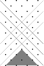
Figure 10. The complex ${{CF^{\infty}}}(E)$. Differentials coming from the top vertex of the shaded triangle must land inside the shaded region.

Proposition 4.1.

The Alexander grading is a filtration on ${{CF_{s}^{\infty}}}({{\mathcal{H}}})$; i.e. if there is a differential from $[{{{\bf y}}},i]$ to $[{{{\bf z}}},j]$ in ${{CF_{s}^{\infty}}}({{\mathcal{H}}})$, $A([{{{\bf y}}},i])\geq A([{{{\bf z}}},j])$.

We refer to this filtration as the Alexander filtration. Note that we do not gain anything more by considering ${{\mathrm{Spin}^{c}}}$ structures other than ${{\mathbf{s}}}_{s}$ and ${{\mathbf{s}}}_{a}$ — the presence of these two filtrations implies the presence of the filtration induced by any ${{\mathbf{s}}}_{k}$.

The fact that the Alexander grading is a filtration can also be derived from the following useful formula for a disk $\phi\in\pi_{2}({{{\bf y}}},{{{\bf z}}})$:

$$n_{z_{a}}(\phi)-n_{z_{s}}(\phi)=A({{{\bf y}}})-A({{{\bf z}}}).$$

Remark: It is easy to check that the map $f$ of Lemma 4.2 respects the Alexander filtration. This implies that the complexes ${{CF^{+}}}({{\mathcal{H}}},n^{\prime},E,{{\mathbf{s}}}_{k})$ are isomorphic for all sufficiently large $n^{\prime}$ and good $\epsilon$–classes, thus justifying our omission of $n^{\prime}$ and $E$ from the notation.

4.5. The reduced stable complex

As a special case of Proposition 4.1, the Alexander grading induces a filtration on ${{\widehat{CF}_{s}}}({{\mathcal{H}}})$. From this filtration we get a spectral sequence $({{\mathcal{S}}}_{i}({{\mathcal{H}}}),d_{i})$ which converges to ${{\widehat{HF}}}(N(n,1),{{\mathbf{s}}}_{s})\cong{{\widehat{HF}}}({{\overline{N}}},{{\overline{{{\mathbf{s}}}}}})$. This sequence is an object of considerable interest: many of the results described below could also be phased in terms of it. For some purposes, however, it is more convenient to have an actual complex, rather than a spectral sequence. For this reason, we introduce the following construction, which we refer to as reduction. Suppose $C$ is a filtered complex with filtration $C_{1}\subset C_{2}\subset\ldots C_{m}$, and let $C^{i}=C_{i+1}/C_{i}$ be the filtered quotients. The homology groups $H_{*}(C^{i})$ are the $E_{2}$ terms of the spectral sequence associated to the filtration.

Lemma 4.5.

Let $C$ be a filtered complex over a field. Then up to isomorphism there is a unique filtered complex $C^{\prime}$ with the following properties:

1. $C^{\prime}$ is chain homotopy equivalent to $C$.

2. $C^{\prime i}\cong H_{*}(C^{i})$

3. The spectral sequence of the filtration on $C^{\prime}$ has trivial first differential. Its higher terms are the same as the higher terms of the spectral sequence of the filtration on $C$.

We refer to $C^{\prime}$ as the reduction of $C$.

The proof will be given in section 5.1.

Definition 4.3.

The reduced stable complex ${{\widehat{CF}_{r}}}(N,m,{{\mathbf{s}}})$ is the reduction of ${{\widehat{CF}_{s}}}({{\mathcal{H}}})$.

The intuitive picture behind this construction is as follows. Recall that each dot in Figure 10 represents a whole set of generators with some particular Alexander grading. On ${{\widehat{CF}_{s}}}({{\mathcal{H}}})$, we split $d$ into two parts: $d=d^{\prime}+d^{\prime\prime}$, where $d^{\prime}$ preserves the Alexander grading and $d^{\prime\prime}$ strictly reduces it. Thus $d^{\prime}$ involves those differentials which “stay within” a given dot, while $d^{\prime\prime}$ contains those differentials which go from one dot to another. The condition $d^{2}=0$ implies that $(d^{\prime})^{2}=0$ as well, so each dot is itself a little chain complex. The idea is to find a new complex chain homotopy equivalent to ${{\widehat{CF}_{s}}}({{\mathcal{H}}})$ in which we have replaced the chain complex inside each dot by its homology.

Our motivation for considering ${{\widehat{CF}_{r}}}$ instead of ${{\widehat{CF}_{s}}}$ is that the new complex is actually a topological invariant:

Theorem 4.

The filtered complex ${{\widehat{CF}_{r}}}(N,m,{{\mathbf{s}}})$ is an invariant of the triple $(N,m,{{\mathbf{s}}})$.

The proof will be given in section 5. For the moment, we remark that the theorem is a specific instance of the general principle that the higher terms of spectral sequences tend to be topological invariants. (A more familiar example of this phenomenon is provided by the Leray-Serre sequence of a fibration, in which the $E_{1}$ term depends on the triangulations of the base and fibre, but the $E_{2}$ and higher terms are canonically defined in terms of the homology of these spaces.)

We record some elementary facts about the reduced stable complex below:

Proposition 4.2.

The reduced stable complex ${{\widehat{CF}_{r}}}(N,m,{{\mathbf{s}}})$ has the following properties:

1. Its homology is isomorphic to ${{\widehat{HF}}}({{\overline{N}}},{{\mathbf{s}}})$.

2. The filtered subquotient ${{\widehat{CF}_{r}}}^{(j)}(N,m,{{\mathbf{s}}})$ is isomorphic to ${{\mathcal{S}}}^{j}_{2}({{\mathcal{H}}})$. Its Euler characteristic is the coefficient of $t^{j}$ in the Alexander polynomial $\Delta(N,m,{{\mathbf{s}}})$.

3. ${{\widehat{CF}_{r}}}(-N,m,{{\mathbf{s}}})$ is the dual complex to ${{\widehat{CF}_{r}}}(N,m,{{\mathbf{s}}})$.

Proof.

Parts 1) and 2) follow from the definition of reduction, combined with Lemma 4.2 and Corollary 3.2, respectively.

To prove part 3), recall that if $(\Sigma,\alpha,\beta)$ is a Heegaard splitting for $N$, $(-\Sigma,\alpha,\beta)$ is a splitting for $-N$. There is an obvious bijection between the elements of good $\epsilon$-classes $E_{\pm N}$ for these splittings, and the Alexander grading on $E_{-N}$ is $-1$ times the Alexander grading on $E_{N}$. Combining this fact with the isomorphisms

$${{\widehat{CF}_{s}}}({{\mathcal{H}}},{{\mathbf{s}}})\cong{{\widehat{CF}}}({{\mathcal{H}}},{{\overline{N}}},z_{s},{{\overline{{{\mathbf{s}}}}}})\cong({{\widehat{CF}}}({{\mathcal{H}}},-{{\overline{N}}},z_{s},{{\overline{{{\mathbf{s}}}}}}))^{*}\cong({{\widehat{CF}_{s}}}(-{{\mathcal{H}}},{{\mathbf{s}}}))^{*}$$

provided by Lemma 4.2 and Proposition 7.3 of [19], we see that ${{\widehat{CF}_{s}}}({{\mathcal{H}}},{{\mathbf{s}}})$ is dual to ${{\widehat{CF}_{s}}}(-{{\mathcal{H}}},{{\mathbf{s}}})$ as a filtered complex. The result then follows from the fact that the dual of the reduction is the reduction of the dual, which will be obvious from the construction of section 5.1. ∎

The first part of the proposition is particularly useful when $(N,m)$ is a knot complement in $S^{3}$, so that ${{\widehat{HF}}}({{\overline{N}}})\cong{{\widehat{HF}}}(S^{3})\cong{\bf{Z}}$.

Definition 4.4.

If $K$ is a knot in $S^{3}$, the level of the generator of $K$, written $s(K)$, is the Alexander grading of the surviving copy of ${\bf{Z}}$ in ${{\mathcal{S}}}_{\infty}({{K^{o}}},m)$.

By Theorem 4, $s(K)$ is an invariant of $K$. Part 4) of the proposition implies that $s(-K)=-s(K)$. We will see in section 7 that this invariant encodes useful information about the exact triangle for surgery on $K$.

It is not difficult to see that everything we have done using the stable complex works just as well when applied to the antistable complex: the Alexander grading $A_{{{\mathbf{s}}}_{a}}=-A$ gives a filtration on ${{\widehat{CF}_{a}}}({{\mathcal{H}}},{{\mathbf{s}}})$, there is a spectral sequence $({{\mathcal{S}}}^{a}_{i},d^{a}_{i})$ derived from it, and the reduced complex ${{\widehat{CF}_{r}}}^{a}$ is a topological invariant. How is this new object related to ${{\widehat{CF}_{r}}}$? Since the first differential in each spectral sequence preserves the Alexander grading, it is easy to see that $({{\mathcal{S}}}^{a}_{2})^{j}\cong{{\mathcal{S}}}_{2}^{-j}$. Thus the two complexes have the same filtered subquotients (but in opposite orders.) Somewhat less obviously, we have

Proposition 4.3.

$${{\widehat{CF}_{r}}}^{a}(N,m,{{\mathbf{s}}})\cong{{\widehat{CF}_{r}}}(N,m,-{{\mathbf{s}}})$$

as filtered complexes.

Proof.

The basic idea is to combine the identification ${{\widehat{CF}_{s}}}({{\mathcal{H}}},{{\mathbf{s}}})\cong{{\widehat{CF}}}({{\mathcal{H}}},{{\overline{N}}},z_{s},{{\overline{{{\mathbf{s}}}}}})$ with the conjugation symmetry ${{\widehat{HF}}}({{\overline{N}}},{{\overline{{{\mathbf{s}}}}}})\cong{{\widehat{HF}}}({{\overline{N}}},-{{\overline{{{\mathbf{s}}}}}})$. The latter isomorphism is realized by simultaneously reversing the orientation of $\Sigma$ and switching the roles of $\alpha$ and $\beta$ in a Heegaard splitting.

With this in mind, we consider the Heegaard splitting $-{{\mathcal{H}}}=(-{\Sigma},\beta,\alpha)$ of $N(n,1)$. There is an obvious identification between ${{\widehat{CF}}}({{\mathcal{H}}},E,z_{a})$ and ${{\widehat{CF}}}(-{{\mathcal{H}}},E,z_{a})$. We will show that the latter complex is actually of the form ${{\widehat{CF}_{s}}}({{\mathcal{H}}}^{\prime},-{{\mathbf{s}}})$ for some new choice of Heegaard data ${{\mathcal{H}}}^{\prime}$. Reducing both sides and applying Theorem 4 gives the desired isomorphism.

By Lemma 3.4 we can assume that our original $m$ has a single geometric intersection with $\alpha_{g}$. In this case, $\alpha_{g}$ and $\beta_{g}$ are mirror-symmetric in the spiral region. This is not obvious from our usual way of drawing the spiral, but if we view the annulus as a cylinder and twist the ends, we can put $\alpha_{g}$ and $\beta_{g}$ into the form of Figure 11, in which the symmetry is overt.

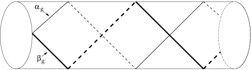
Figure 11. The curves $\alpha_{g}$ and $\beta_{g}$ in the spiral region.

Thus our new Heegaard splitting $-{{\mathcal{H}}}$ has the form we used to define the stable complex: the new $\beta_{g}$ (which used to be $\alpha_{g}$) has been twisted around $m$ many times in a positive sense. It is not difficult to see that $E$ is a good $\epsilon$-class for this new splitting, and since we reversed the orientation of $\Sigma$, the basepoint $z_{a}$ is actually on the stable side of the new complex. The only thing remaining to check is that the manifold that we get by omitting $\alpha_{g}$ from $-{{\mathcal{H}}}$ is still $N$. For this, we use

Lemma 4.6.

Suppose $(\Sigma,\alpha,\beta)$ is a Heegaard splitting of $Y$, and $m\subset Y$ is represented by a curve on $\Sigma$ which intersects $\beta_{g}$ geometrically once and misses all of the other $\beta_{i}$’s. Then $(\Sigma,\alpha,\beta_{1},\ldots,\beta_{g-1})$ is a Heegaard splitting of $N-m$.

Proof.

If we push $m$ off of $\Sigma$, we see that it punches a single hole in the handle attached along $\beta_{g}$ and misses the other $\beta$ handles. To get the desired splitting, we retract what is left of the $\beta_{g}$ handle back to $\Sigma$. ∎

Applying the lemma to the two splittings ${{\mathcal{H}}}$ and $-{{\mathcal{H}}}$ of $N(n,1)$, we see that omitting $\alpha_{g}$ from $-{{\mathcal{H}}}$ gives the same manifold as omitting $\beta_{g}$ from ${{\mathcal{H}}}$. Since latter manifold is $N$, the claim is proved. ∎

Thus we do not get any new invariants by considering the antistable complex. What we do get, however, is an extension of the usual conjugation symmetry on ${{\widehat{HF}}}$ to the stable complex. For example, when $N={{K^{o}}}$ is a knot complement, the proposition implies that ${{\mathcal{S}}}_{2}^{j}(K)\cong{{\mathcal{S}}}_{2}^{-j}(K)$. This fact can very helpful in practice, since one of the ${{\mathcal{S}}}_{2}^{\pm j}$ may be easier to compute than the other.

To make full use of the symmetry between stable and antistable complexes, it is convenient to introduce yet another affine grading on $E$:

Definition 4.5.

For ${{{\bf y}}}\in E$, we set ${{\tilde{\mu}}}({{{\bf y}}})={{\mathrm{gr}}}_{{{\mathbf{s}}}_{k}}({{{\bf y}}})-A_{{{\mathbf{s}}}_{k}}({{{\bf y}}})$.

The important point is that ${{\tilde{\mu}}}$ does not depend on which ${{\mathbf{s}}}_{k}$ we use. This is obvious if we think of ${{\widehat{CF}}}({{\mathcal{H}}},{{\mathbf{s}}}_{k})$ as a subset of ${{CF_{s}^{\infty}}}({{\mathcal{H}}})$: the difference ${{\mathrm{gr}}}([{{{\bf y}}},j])-A([{{{\bf y}}},j])$ is clearly independent of $j$. This fact gives us an easy way to compute all the ${{\mathrm{gr}}}_{{{\mathbf{s}}}_{k}}$’s from any one of them.

Since it depends only on the Alexander and homological gradings, the definition of $\tilde{\mu}$ makes sense for for a generator of ${{\widehat{CF}_{r}}}$ as well. Suppose that $N={{K^{o}}}$ is a knot complement, and set

$$C(K,j,l)=\{{{{\bf y}}}\in{{\widehat{CF}_{r}}}(K){{\thinspace}}|{{\thinspace}}A({{{\bf y}}})=j,{{\thinspace}}\tilde{\mu}({{{\bf y}}})=l\}$$

The symmetry between ${{\mathcal{S}}}_{2}^{j}$ and ${{\mathcal{S}}}_{2}^{-j}$ implies that $C(K,j,l)\cong C(K,-j,l)$. Thus from the point of view of ${{\mathrm{gr}}}_{{{\mathbf{s}}}_{s}}$, ${{\widehat{CF}_{r}}}(K)$ is composed of symmetrical pieces on which $\tilde{\mu}$ is constant, but these pieces are put together in such a way that ${{\mathrm{gr}}}_{{{\mathbf{s}}}_{s}}$ is not symmetric on ${{\widehat{CF}_{r}}}(K)$. (See the discussion of the $(3,5)$ torus knot below for an example of such a decomposition.)

We conclude our discussion of the reduced stable complex by describing ${{\widehat{CF}_{r}}}(K)$ for two basic types of knots. Example 1: Two-bridge knots If $K$ is a two-bridge knot with the two-bridge Heegaard splitting, ${{\mathrm{gr}}}_{{{\mathbf{s}}}_{s}}=A$. Since every differential reduces the Alexander grading by one, ${{\widehat{CF}_{r}}}(K)\cong{{\widehat{CF}_{s}}}({{\mathcal{H}}})$, and the rank of ${{\mathcal{S}}}^{2}_{j}(K)$ is the absolute value of the coefficient of $t^{j}$ in $\Delta_{K}(t)$. In addition, $s(K)=\sigma(K)/2$, where $\sigma$ is the ordinary knot signature. Thus the isomorphism class of ${{\widehat{CF}_{r}}}(K)$ is completely determined by classical knot invariants. For two-bridge knots, the symmetry of ${{\widehat{CF}_{r}}}(K)$ is explicitly realized by a natural involution of the Heegaard splitting, as described in [25]. Example 2: Torus knots If $K=T(p,p+1)$ is the right-handed $(p,p+1)$ torus knot, the coefficients of $\Delta_{K}(t)$ are always $\pm 1$ or $0$. We show in the appendix that the rank of ${{\mathcal{S}}}(K)_{2}^{j}$ is the absolute value of the corresponding coefficient of $\Delta_{K}(t)$. Let ${{{\bf y}}}_{1},{{{\bf y}}}_{2},\ldots,{{{\bf y}}}_{m}$ be the generators of ${{\widehat{CF}_{r}}}(K)$ arranged in order of decreasing Alexander grading. Then there is a differential from ${{{\bf y}}}_{2i}$ to ${{{\bf y}}}_{2i+1}$. The presence of these differentials enables us to compute ${{\mathrm{gr}}}_{{{\mathbf{s}}}_{s}}$. It turns out that for $i>j$, ${{\mathrm{gr}}}_{{{\mathbf{s}}}_{s}}({{{\bf y}}}_{i})>{{\mathrm{gr}}}_{{{\mathbf{s}}}_{s}}({{{\bf y}}}_{i})$, so the differentials described above are the only differentials in ${{\widehat{CF}_{r}}}(K)$. In turn, this implies that ${{\widehat{HF}_{s}}}(K)$ is generated by ${{{\bf y}}}_{1}$, so $s(T(p,p+1))=g(T(p,p+1))=p(p-1)/2$. We illustrate how to how to find ${{\mathrm{gr}}}_{{{\mathbf{s}}}_{s}}$ in the case of the $(3,5)$ torus knot. The Alexander grading on ${{\widehat{CF}_{r}}}(K)$ is shown in Figure 12a. There is a differential from ${{{\bf y}}}_{2i}$ to ${{{\bf y}}}_{2i+1}$, so

$${{\mathrm{gr}}}_{s}({{{\bf y}}}_{2i})-{{\mathrm{gr}}}_{s}({{{\bf y}}}_{2i+1})=1.$$

On the other hand, the symmetry between stable and antistable complexes shows that in the antistable complex, there must be a differential from ${{{\bf y}}}_{2i}$ to ${{{\bf y}}}_{2i-1}$, so

$${{\mathrm{gr}}}_{a}({{{\bf y}}}_{2i})-{{\mathrm{gr}}}_{a}({{{\bf y}}}_{2i-1})=1.$$

Then we compute, for example, that ${{\tilde{\mu}}}({{{\bf y}}}_{6},{{{\bf y}}}_{5})=-1$, so ${{\mathrm{gr}}}_{s}({{{\bf y}}}_{6},{{{\bf y}}}_{5})=-3$. The other gradings can be found by the same method.

Figure 12.

The reduced stable complex of the $(3,5)$ torus knot, showing the (a) Alexander and (b) homological gradings of the generators.

4.6. Reduction for ${{CF_{s}^{\infty}}}({{\mathcal{H}}})$

There is no reason that the process of reduction should be limited to the stable complex. In fact, there are reduced versions of the all the various Ozsváth-Szabó  Floer complexes. We briefly describe these other reduced complexes and their relation to the reduced stable complex. Since the complex ${{CF_{s}^{\infty}}}({{\mathcal{H}}},{{\mathbf{s}}})$ contains all of the others, it is a natural place to start. We filter ${{CF_{s}^{\infty}}}({{\mathcal{H}}},{{\mathbf{s}}})$ by the Alexander grading and denote the associated reduced complex by ${{CF_{r}^{\infty}}}({{\mathcal{H}}},{{\mathbf{s}}})$. (This is not a finite filtration, but it is finitely supported in each degree, so it is still possible to take the reduction.)

Lemma 4.7.

As a group, ${{CF_{r}^{\infty}}}({{\mathcal{H}}})\cong\bigoplus_{i,j}{{\thinspace}}[{{\mathcal{S}}}_{2}^{i}({{\mathcal{H}}},{{\mathbf{s}}}),j]$.

Proof.

Let $C^{l}$ be the subquotient of ${{CF_{s}^{\infty}}}({{\mathcal{H}}},{{\mathbf{s}}})$ generated by the elements of Alexander grading $l$. It is easy to see from Figure 10 that as a complex,

$$C^{l}=\oplus_{i+2j=l}{{\thinspace}}[{{\mathcal{S}}}_{1}^{i}({{\mathcal{H}}},{{\mathbf{s}}}),j].$$

∎

${{CF_{r}^{\infty}}}({{\mathcal{H}}},{{\mathbf{s}}})$ retains the same double filtration structure as ${{CF_{s}^{\infty}}}({{\mathcal{H}}},{{\mathbf{s}}})$, so it has subcomplexes ${{CF_{r}^{-}}}({{\mathcal{H}}},{{\mathbf{s}}}_{k})$ and quotient complexes ${{CF_{r}^{+}}}({{\mathcal{H}}},{{\mathbf{s}}}_{k})$ specified by the same sets of dots as ${{CF^{-}}}({{\mathcal{H}}},{{\mathbf{s}}}_{k})$ and ${{CF^{+}}}({{\mathcal{H}}},{{\mathbf{s}}}_{k})$. We would like to know that these complexes are the same as those obtained by reducing ${{CF^{\pm}}}({{\mathcal{H}}},{{\mathbf{s}}}_{k})$. This is implied by the following lemma, which will be proved in section 5.1:

Lemma 4.8.

Suppose $B$ is a filtered complex, and that there is a short exact sequence

$$\begin{CD}0@>{}>{}>A@>{}>{}>B@>{}>{}>C@>{}>{}>0\end{CD}$$

which respects the filtration, in the sense that $B^{i}=A^{i}\oplus C^{i}$ (as complexes). Then there is a commutative diagram

$$\setcounter{MaxMatrixCols}{11}\begin{CD}0@>{}>{}>A@>{}>{}>B@>{}>{}>C@>{}>{}>0\\ @V{}V{}V@V{}V{}V@V{}V{}V@V{}V{}V@V{}V{}V\\ 0@>{}>{}>A^{r}@>{}>{}>B^{r}@>{}>{}>C^{r}@>{}>{}>0\end{CD}$$

in which the vertical arrows are homotopy equivalences.

Thus as far as the homology is concerned, there is no difference between using the reduced complexes and their unreduced counterparts. Similarly, we can view the reduced complex ${{\widehat{CF}_{r}}}({{\mathcal{H}}},{{\mathbf{s}}}_{k})$ as a subcomplex of ${{CF_{r}^{+}}}({{\mathcal{H}}},{{\mathbf{s}}}_{k})$.

In analogy with Theorem 1, we expect that all of these reduced complexes should also be topologically invariant. The next proposition shows that this is true for ${{\widehat{CF}_{r}}}({{\mathcal{H}}},{{\mathbf{s}}}_{k})$. For the others, some more careful accounting in the proof of Theorem 1 might provide a proof. (This is done in [23].) Since we do not have any immediate need for this invariance, however, we will not pursue the matter here.

We can use our knowledge of ${{\widehat{CF}_{r}}}(N,m,{{\mathbf{s}}})$ and ${{\widehat{CF}_{a}}}(N,m,{{\mathbf{s}}})$ to understand some of the differentials in the other reduced complexes. For example, if $N={{K^{o}}}$ is a knot complement, and we let $S_{k}(K)$ be the subcomplex of ${{\widehat{CF}_{r}}}(K)$ generated by those elements with Alexander grading less than $k$, then we have

Proposition 4.4.

There is a short exact sequence

$$\begin{CD}0@>{}>{}>S_{-k}(K)\oplus S_{k}(K)@>{}>{}>{{\widehat{CF}_{r}}}(K,{{\mathbf{s}}}_{k})@>{}>{}>{{\mathcal{S}}}_{2}^{k}(K)@>{}>{}>0.\end{CD}$$

Proof.

It is clear from Figure 13 that we have a short exact sequence

$$\begin{CD}0@>{}>{}>A\oplus C@>{}>{}>{{\widehat{CF}_{r}}}(K,{{\mathbf{s}}}_{k})@>{}>{}>B@>{}>{}>0\end{CD}$$

If we think of everything as being inside ${{CF_{r}^{\infty}}}({{\mathcal{H}}})$, we see that $C\cong S_{k}(K)$ and $B\cong{{\mathcal{S}}}_{2}^{k}(K)$. To identify $A$ with $S_{-k}(K)$, we use the isomorphism ${{\widehat{CF}_{r}}}(K)\cong{{\widehat{CF}_{a}}}(K)$. ∎

Figure 13. A dot picture of ${{\widehat{HF}}}({{\mathbf{s}}}_{k})$

In general, if we know the filtered complexes ${{\widehat{CF}_{r}}}(N,m,{{\mathbf{s}}})$ and ${{\widehat{CF}_{r}}}(N,m,-{{\mathbf{s}}})$ we can deduce the structure of ${{\widehat{CF}_{r}}}(N,m,{{\mathbf{s}}}_{k})$ for every ${{\mathbf{s}}}_{k}$. The situation for ${{CF_{r}^{\infty}}}({{\mathcal{H}}},{{\mathbf{s}}})$ is more complicated. Knowledge of ${{\widehat{CF}_{r}}}(N,m,{{\mathbf{s}}})$ tells us what the differentials which go to the edge of the shaded triangle in Figure 10 are, but does not give us any information about those differentials which go to the interior.

5. Invariance of ${{\widehat{CF}_{r}}}$

The first goal of this section is to explain the process of reduction, show that it is well defined, and prove that a filtration preserving chain map induces a chain map of the reduced complexes. Once this has been taken care of, we turn to the proof of Theorem 4. We need to show that ${{\widehat{CF}_{r}}}$ is does not depend on the various choices we have made in defining it, such as the Heegaard splitting of $N$, the geometric representative of the meridian, and the position of the basepoint $z$. In each case, we examine the proof of invariance of ${{\widehat{HF}}}$ given in [19] and check that it can be adapted to show that ${{\widehat{CF}_{r}}}$ is invariant as well.

As an example of how this process works, suppose we transform the Heegaard diagram ${{\mathcal{H}}}$ into a new diagram ${{\mathcal{H}}}^{\prime}$ by a handleslide. Ozsváth and Szabó exhibit a chain map $F{{\colon}}{{\widehat{CF}}}({{\mathcal{H}}})\to{{\widehat{CF}}}({{\mathcal{H}}}^{\prime})$ and show that the induced map on homology is an isomorphism. From our perspective, the key point is that since $F$ is defined using holomorphic triangles, it preserves the Alexander filtration. Thus there are induced maps $F^{i}{{\colon}}{{\mathcal{S}}}_{1}^{i}({{\mathcal{H}}})\to{{\mathcal{S}}}_{1}^{i}({{\mathcal{H}}}^{\prime})$. The argument used to show that ${{\widehat{HF}}}$ is invariant under handleslide actually implies that the maps $F^{i}_{*}{{\colon}}{{\mathcal{S}}}_{2}^{i}({{\mathcal{H}}})\to{{\mathcal{S}}}_{2}^{i}({{\mathcal{H}}}^{\prime})$ are isomorphisms. It is a standard fact (see e.g. Theorem 3.1 of [15]) that this implies that all the higher terms in the spectral sequence are the same as well. It also enables us to show that the associated reduced complexes are isomorphic.

5.1. Reducing a filtered complex

Throughout this section, we work with field coefficients. Recall the setup of Lemma 4.5: we have a complex $(C,d)$ with a filtration $C_{1}\subset C_{2}\ldots\subset C_{m}$ and filtered quotients $(C^{i},d^{i})=C_{i+1}/C_{i}$. We wish to find an equivalent complex $(C^{\prime},d^{\prime})$ such that $d^{\prime i}\equiv 0$. The basic tool is the well-known “cancellation lemma”:

Lemma 5.1.

Suppose $(C,d)$ is a chain complex freely generated by elements $y_{i}$, and write $d(y_{i},y_{j})$ for the $y_{j}$ coordinate of $d(y_{i})$. Then if $d(y_{k},y_{l})=1$, we can define a new complex $(\overline{C},\overline{d})$ with generators $\{y_{i}{{\thinspace}}|{{\thinspace}}i\neq k,l\}$ and differential

$$\overline{d}(y_{i})=d(y_{i})+d(y_{i},y_{l})d(y_{k})$$

which is chain homotopy equivalent to the first one.

Remarks: A proof of this fact may be found in [4]. The chain homotopy equivalence $\pi{{\colon}}C\to\overline{C}$ is just the projection, while the equivalence $\iota{{\colon}}\overline{C}\to C$ is given by $\iota(y_{i})=y_{i}-d(y_{i},y_{l})y_{k}$.

Proof.

(Of Lemma 4.5) If all the $d^{i}$ are $0$, the result obviously holds. If not, we can find $x,y\in C^{i}$ with $d^{i}(x,y)\neq 0$. Since we are using field coefficients, we can assume that $x$ and $y$ are generators of $C$ and scale $y$ so that $d^{i}(x,y)=1$. This implies that $d(x,y)=1$ as well, so we can apply the cancellation lemma to obtain a new complex $(\overline{C},\overline{d})$ chain homotopy equivalent to our original $C$.

We claim that the filtration on $C$ induces a filtration on $\overline{C}$. Indeed, suppose that

$$\overline{d}(u,v)=d(u,v)+d(u,y)d(x,v)\neq 0.$$

Then either $d(u,v)\neq 0$, which implies that $u\geq v$, or $d(u,y)d(x,v)\neq 0$, which implies $u\geq y$ and $x\geq v$. By hypothesis, $x$ and $y$ have the same filtration, so $u\geq v$ in this case as well. Moreover, the chain homotopy equivalences $\iota$ and $\pi$ are filtered maps. This is obvious for $\pi$, and is true for $\iota$ because $d(u,y)\neq 0$ implies that $u\geq y\geq x$.

The maps $\iota_{*}^{j}{{\colon}}H_{*}(\overline{C}^{j})\to H_{*}(C^{j})$ and $\pi_{*}^{j}{{\colon}}H_{*}({C}^{j})\to H_{*}(\overline{C}^{j})$ are isomorphisms. Indeed, when $j\neq i$, it is easy to see that $d^{j}=\overline{d}^{j}$. On the other hand, $\overline{C}^{i}$ is just the complex obtained from $C^{i}$ by cancelling $x$ and $y$. It follows that $\iota$ and $\pi$ induce an isomorphisms on the $E_{2}$ terms of the spectral sequences for $C$ and $\overline{C}$. It is then a standard fact (see e.g. Theorem 3.1 of [15]) that they induce isomorphisms on all higher terms as well.

We now repeat this process. Since $C$ was finitely generated, the cancellation must terminate after a finite number of steps. The result is the desired complex $(C^{\prime},d^{\prime})$. To show that $C^{\prime}$ is unique up to isomorphism, suppose we have another reduction $(C^{\prime\prime},d^{\prime\prime})$. Then by transitivity, $C^{\prime}$ is chain homotopy equivalent to $C^{\prime\prime}$, and the induced map on the $E_{2}$ terms of the spectral sequences is an isomorphism. It follows that the map $C^{\prime}\to C^{\prime\prime}$ is an isomorphism at the level of groups. But a chain map which is an isomorphism on groups is an isomorphism of chain complexes. ∎

The following lemma says that we can reduce maps as well as complexes:

Lemma 5.2.

Suppose $f{{\colon}}C\to D$ is a filtration preserving map. Then there is an induced map $f^{\prime}{{\colon}}C^{\prime}\to D^{\prime}$. Moreover, $f$ and $f^{\prime}$ induce the same maps on spectral sequences.

Proof.

Choose chain homotopy equivalences $\iota{{\colon}}C^{\prime}\to C$ and $\pi{{\colon}}D\to D^{\prime}$, and set $f^{\prime}=\pi\circ f\circ\iota$. Since $\iota$ and $\pi$ induce isomorphisms on spectral sequences, the map on spectral sequences induced by $f^{\prime}$ is the same as the map induced by $f$. ∎

We would also like to know that the reduced map $f^{\prime}$ is unique. Since we have only defined the reduced complex up to isomorphism, the best we can hope to show is that any two reductions $f^{\prime}$ and $f^{\prime\prime}$ differ by composition with isomorphisms at either end. This is indeed the case. Supppose, for example, that $\iota_{1}{{\colon}}C^{\prime}\to C$ is another chain homotopy equivalence, and let $\pi_{1}$ be its homotopy inverse. Then $\iota$ is chain homotopic to $\iota_{1}\circ\pi_{1}\circ\iota$, and $\pi_{1}\circ\iota$ is an isomorphism from $C^{\prime}$ to itself. Finally, $\pi\circ f\circ\iota$ is equal (not just homotopic!) to $\pi\circ f\circ\iota_{1}\circ(\pi_{1}\circ\iota)$, since both sides induce the same map on $E_{2}$ terms of spectral sequences. A similar argument handles the case of a different $j$.

It is now easy to prove Lemma 4.8:

Proof.

Suppose $x,y\in B^{i}$ are a pair of cancelling elements, as in the proof of Lemma 4.5. Since $B^{i}\cong A^{i}\oplus C^{i}$, $x$ and $y$ are either both in $A^{i}$ or both in $C^{i}$. For the moment, we suppose the former. Then for $u\in A$, it is easy to see that $\overline{d}|_{A}$ is the same as the differential obtained by cancelling $x$ and $y$ in $A$. On the other hand, if $z,w\in B\backslash A$, $\overline{d}(z,w)=d(z,w)$. Thus we have a commutative diagram

$$\setcounter{MaxMatrixCols}{11}\begin{CD}0@>{}>{}>A@>{}>{}>B@>{}>{}>C@>{}>{}>0\\ @V{}V{}V@V{}V{}V@V{}V{}V@V{}V{}V@V{}V{}V\\ 0@>{}>{}>\overline{A}@>{}>{}>\overline{B}@>{}>{}>C@>{}>{}>0\end{CD}$$

in which the vertical arrows are chain homotopy equivalences. If $x,y$ are in $C$, there is similar diagram involving $A$, $\overline{B}$ and $\overline{C}$. We now repeat, stacking the diagrams on top of each other as we go. Compressing the resulting large diagram gives the statement of the lemma. ∎

5.2. Filtered chain homotopies

Let $C$ and $D$ be chain complexes. A map $i{{\colon}}C\to D$ is a chain homotopy equivalence if there exists a homotopy inverse $j{{\colon}}D\to C$, and chain homotopies $H_{1}{{\colon}}C\to C$, $H_{2}{{\colon}}D\to D$ such that

(2) $$1_{C}-ji =dH_{1}-H_{1}d$$

(3) $$1_{D}-ij =dH_{2}-H_{2}d$$

Now suppose that that $C$ and $D$ are both filtered complexes. We say that $i$ is a filtered chain homotopy equivalence if $i,j,H_{1}$, and $H_{2}$ all respect the filtration.

Lemma 5.3.

Let $i:C\to D$ be a filtered chain homotopy equivalence. Then all the induced maps $i^{k}:C^{k}\to D^{k}$ are chain homotopy equivalences as well.

Proof.

Since $i,j,H_{1}$ and $H_{2}$ all respect the filtration, they induce maps $i^{k},j^{k},H_{1}^{k}$, and $H_{2}^{k}$ on the filtered quotients. It is easy to see that the analogues of equations 2 and 3 hold for these maps as well. ∎

We can now explain the strategy for proving Theorem 4 in a bit more detail. First, we list the choices we made in defining ${{\widehat{CF}_{s}}}({{\mathcal{H}}})$:

1. A generic path of almost-complex structures $J_{s}$ on $s^{g}\Sigma$ and a generic complex structure ${{\mathfrak{j}}}$ on $\Sigma$.

2. A Heegaard splitting of $N$.

3. The geometric representative ${{\mathfrak{m}}}$ of $m$.

4. The position of the basepoint $z$.

If we change any one of these things, we get a new stable complex, which we denote by ${{\widehat{CF}_{s}}}({{\mathcal{H}}}^{\prime})$. Now in many cases, the proof in [19] that ${{\widehat{HF}}}$ is a topological invariant gives us a chain homotopy equivalence $i{{\colon}}{{\widehat{CF}}}({{\mathcal{H}}})\to{{\widehat{CF}}}({{\mathcal{H}}}^{\prime})$. In the sections below, we check that $i$ is actually a filtered chain homotopy equivalence. Assuming that this is the case, the remainder of the proof is straightforward. Indeed, Lemma 5.3 tells us that $i$ induces isomorphisms $i^{k}{{\colon}}{{\mathcal{S}}}_{2}^{k}({{\mathcal{H}}})\to{{\mathcal{S}}}_{2}^{k}({{\mathcal{H}}}^{\prime})$. It follows that the induced map $i^{\prime}{{\colon}}{{\widehat{CF}_{r}}}({{\mathcal{H}}})\to{{\widehat{CF}_{r}}}({{\mathcal{H}}}^{\prime})$ is an isomorphism at the level of groups, which implies that ${{\widehat{CF}_{r}}}({{\mathcal{H}}})\cong{{\widehat{CF}_{r}}}({{\mathcal{H}}}^{\prime})$.

As a model case, let us check that ${{\widehat{CF}_{r}}}$ does not depend on $J_{s}$ or ${{\mathfrak{j}}}$. This is proved for ${{\widehat{HF}}}$ in Lemma 4.9 of [19], using a standard argument in Floer theory. Given two paths $J_{s}(0)$ and $J_{s}(1)$, one connects them by a generic homotopy of paths $J_{s}(t)$ and defines a chain homotopy equivalence $\Phi_{J_{s,t}}{{\colon}}{{\widehat{CF}}}({{\mathcal{H}}})\to{{\widehat{CF}}}({{\mathcal{H}}}^{\prime})$ by

$$\Phi_{J_{s,t}}({{{\bf y}}})=\sum_{{{{\bf z}}}}\sum_{\phi\in D}\#{\widehat{\mathcal{M}}}_{J_{s,t}}(\phi)\cdot{{{\bf z}}}$$

where $D=\{\phi\in\pi_{2}({{{\bf y}}},{{{\bf z}}}){{\thinspace}}|{{\thinspace}}\mu(\phi)=n_{z_{s}}(\phi)=0\}$ and ${\widehat{\mathcal{M}}}_{J_{s,t}}(\phi)$ is the moduli space of time dependent holomorphic strips associated to the path $J_{s}(t)$. The domain of such a $\phi$ looks just like the domain of a differential (except that it has Maslov index 0), so $n_{z_{a}}(\phi)-n_{z_{s}}(\phi)=A({{{\bf y}}})-A({{{\bf z}}})$. Since $n_{z_{s}}(\phi)=0$, we must have $A({{{\bf y}}})\geq A({{{\bf z}}})$ whenever ${{{\bf z}}}$ has a nonzero coefficient in the sum. Thus $\Phi_{J_{s,t}}$ is a filtration preserving map. Its homotopy inverse $\Phi_{J_{s,1-t}}$ is also filtration preserving (by the same argument). The chain homotopy between $\Phi_{J_{s,t}}\circ\Phi_{J_{s,1-t}}$ and the identity is given by

$$H_{J_{s,t,\tau}}=\sum_{{{{\bf z}}}}\sum_{\phi\in D^{\prime}}\#{\widehat{\mathcal{M}}}_{J_{s,t,\tau}}(\phi)\cdot{{{\bf z}}}$$

where $J_{s,t,\tau}$ is a suitable two parameter family of almost complex structures and $D^{\prime}=\{\phi\in\pi_{2}({{{\bf y}}},{{{\bf z}}}){{\thinspace}}|{{\thinspace}}\mu(\phi)=-1,{{\thinspace}}n_{z_{s}}(\phi)=0\}$. It is easy to see that $H_{J_{s,t,\tau}}$ is also filtration preserving. Thus Lemma 5.3 applies, and we conclude that ${{\widehat{CF}_{r}}}({{\mathcal{H}}})\cong{{\widehat{CF}_{r}}}({{\mathcal{H}}}^{\prime})$. The argument used in [19] to show that ${{\widehat{HF}}}$ is independent of the generic almost complex structure ${{\mathfrak{j}}}$ on $\Sigma$ carries over without change to ${{\widehat{CF}_{r}}}$.

In the following sections, we use arguments like this one to show that ${{\widehat{CF}_{r}}}$ is invariant under isotopies, handleslides, stabilizations, and changes of basepoint. Finally, in section 5.7, we put these results together to prove the theorem.

5.3. Isotopy invariance

Proposition 5.1.

${{\widehat{CF}_{r}}}$ is invariant under isotopies of ${{\mathfrak{m}}}$, $\alpha_{i}$, and $\beta_{j}$ supported away from $z_{s}$.

Proof.

If the isotopy does not create or destroy intersections, it is equivalent to an isotopy of the conformal structure on $\Sigma$. We observed above that ${{\widehat{CF}_{r}}}$ is invariant under such isotopies. Thus it suffices to consider the case in which a pair of intersection points between ${{\mathfrak{m}}}$ or one of the $\beta_{j}$’s and one of the $\alpha_{i}$’s is created or destroyed. Since an isotopy that moves $\beta_{j}$ over $\alpha_{i}$ is indistinguishable from one that moves $\alpha_{i}$ over $\beta_{j}$, we assume without loss of generality that the curve that is moving is one of the $\alpha_{i}$, and that ${{\mathfrak{m}}}$ and all the $\beta_{j}$’s are fixed.

The isotopy invariance of ${{\widehat{HF}}}$ in this case is proved in Theorem 4.10 of [19]. The argument is as follows. We represent the isotopy of $\alpha_{i}$ by a family of Hamiltonian diffeomorphisms $\Psi_{t}$ of $\Sigma$, and consider the map $F_{\Psi_{t}}{{\colon}}{{\widehat{CF}_{r}}}({{\mathcal{H}}})\to{{\widehat{CF}_{r}}}({{\mathcal{H}}}^{\prime})$ defined by

$$F_{\Psi_{t}}({{{\bf y}}})=\sum_{{{{\bf z}}}\in E^{\prime}}\sum_{\phi\in D}\#{\widehat{\mathcal{M}}}^{\Psi_{t}}(\phi)\cdot{{{\bf z}}}$$

where $D=\{\phi\in\pi_{2}^{\Psi_{t}}({{{\bf y}}},{{{\bf z}}}){{\thinspace}}|{{\thinspace}}\mu(\phi)=n_{z_{s}}(\phi)=0\}$. The moduli space ${\widehat{\mathcal{M}}}^{\Psi_{t}}(\phi)$ counts holomorphic discs subject to an appropriate time dependent boundary condition determined by $\Psi_{t}$. The usual Floer homology arguments show that this is a chain map, and that $F_{\Psi_{1-t}}\circ F_{\Psi_{t}}{{\colon}}{{\widehat{CF}_{r}}}(E)\to{{\widehat{CF}_{r}}}(E)$ is chain homotopic to the identity. The chain homotopy is defined by choosing a homotopy $\Phi_{t,\tau}$ between $\Psi_{1-t}*\Psi_{t}$ and the identity and setting

$$H({{{\bf y}}})=\sum_{{{{\bf z}}}\in E}\sum_{\phi\in D^{\prime}}\#{\widehat{\mathcal{M}}}^{\Phi_{t,\tau}(\phi)}(\phi)\cdot{{{\bf z}}}$$

where $D^{\prime}=\{\phi\in\pi_{2}^{\Phi_{t,\tau}}({{{\bf y}}},{{{\bf z}}}){{\thinspace}}|{{\thinspace}}n_{z_{s}}=0,{{\thinspace}}\mu(\phi)=-1\}$. Notice that this proof never uses the hypothesis that only a single pair of points are created or destroyed. Thus it applies just as well when $\alpha_{i}$ isotopes over a meridian, which creates or destroys many pairs of intersection points in the Heegaard splitting for $N(n,1)$.

To prove invariance, we need to check that $F$ and $H$ preserve the Alexander filtration. We argue much as we did in proving invariance with respect to $J_{s}$. The only real difference is that the ${{\mathcal{D}}}(\phi)$ is a bit more difficult to control, since the $\alpha_{i}$ is only known to lie in $\Psi_{t}(\alpha_{i})$. By hypothesis, however, the isotopy is supported away from $z_{s}$, so the multiplicity $n_{z_{s}}(\phi)$ is well defined for $\phi\in D$ or $D^{\prime}$. It still makes sense to talk about the $\beta_{g}$ component of $\partial{{\mathcal{D}}}(\phi)$, and the usual argument still shows that the $\beta_{g}$ component is supported inside the spiral. Thus $n_{z_{a}}(\phi)=A({{{\bf y}}})-A({{{\bf z}}})$ still holds. Since any $\phi$ with $\#{\widehat{\mathcal{M}}}(\phi)\neq 0$ has $n_{z_{a}}(\phi)\geq 0$, $F$ and $H$ respect the Alexander filtration. The proposition now follows from Lemma 5.3. ∎

5.4. Handleslide invariance

The proof that ${{\widehat{CF}_{r}}}$ is invariant under handleslide is considerably more complicated than the preceding arguments. There are three separate cases to consider. In the first, one of the $\beta$ handles in the Heegaard splitting of $N$ slides over another; in the second, one of the $\alpha$ handles slides over another; in the last, $\mathfrak{m}$ slides over one of the $\beta$ handles in the Heegaard splitting.

We first outline the proof that ${{\widehat{HF}}}$ is invariant under handleslide given by Ozsváth and Szabó in [19]. We adopt their notation, which is as follows: the two original sets of attaching handles will be denoted by $\alpha$ and $\beta$. $\delta$ is a set of attaching handles obtained by small isotopies of the $\beta$ handles, so that each $\beta_{i}$ intersects $\delta_{i}$ at precisely two points. We let $\gamma_{1}$ be the handle obtained by sliding $\beta_{1}$ over $\beta_{2}$. The other $\gamma_{i}$’s are obtained by small isotopies of the $\beta_{i}$’s, so that $\beta_{i}\cap\gamma_{i}$ and $\gamma_{i}\cap\delta_{i}$ each consist of two points. The main steps of the proof in [19] are as follows.

1. Show that ${{\widehat{HF}}}({{\bf T}}_{\beta},{{\bf T}}_{\gamma})\cong{{\widehat{HF}}}({{\bf T}}_{\gamma},{{\bf T}}_{\delta})\cong{{\widehat{HF}}}({{\bf T}}_{\beta},{{\bf T}}_{\delta})\cong H_{*}(T^{g})$. Label the top generators of these three groups $\theta_{1},\theta_{2}$, and $\theta_{3}$ respectively.

2. Define maps

   $$\hat{f}_{\alpha,\beta,\gamma}(\cdot\otimes\theta_{1}){{\colon}}\ {{\widehat{CF}}}({{\bf T}}_{\alpha},{{\bf T}}_{\beta})\to{{\widehat{CF}}}({{\bf T}}_{\alpha},{{\bf T}}_{\gamma})$$

   $$\hat{f}_{\alpha,\gamma,\delta}(\cdot\otimes\theta_{2}){{\colon}}\ {{\widehat{CF}}}({{\bf T}}_{\alpha},{{\bf T}}_{\gamma})\to{{\widehat{CF}}}({{\bf T}}_{\alpha},{{\bf T}}_{\delta})$$

   $$\hat{f}_{\alpha,\beta,\delta}(\cdot\otimes\theta_{3}){{\colon}}\ {{\widehat{CF}}}({{\bf T}}_{\alpha},{{\bf T}}_{\beta})\to{{\widehat{CF}}}({{\bf T}}_{\alpha},{{\bf T}}_{\delta})$$

   by counting holomorphic triangles. For example

   $$\hat{f}_{\alpha,\beta,\gamma}({{{\bf y}}}\otimes\theta_{1})=\sum c({{{\bf y}}},\theta_{1},{{{\bf z}}})\cdot{{{\bf z}}}$$

   where

   $$c({{{\bf y}}},\theta_{1},{{{\bf z}}})=\sum_{\{\psi\in\pi_{2}({{{\bf y}}},\theta_{1},{{{\bf z}}}){{\thinspace}}|{{\thinspace}}\mu(\psi)=n_{z_{s}}(\psi)=0\}}\#{\widehat{\mathcal{M}}}(\psi).$$

   Check that these maps are chain maps, and label the induced maps on homology by $\hat{F}_{\alpha,\beta,\gamma}(\cdot\otimes\theta_{1})$, $\hat{F}_{\alpha,\gamma,\delta}(\cdot\otimes\theta_{2})$, and $\hat{F}_{\alpha,\beta,\delta}(\cdot\otimes\theta_{3})$

3. Prove the associativity relation

   $$\hat{F}_{\alpha,\gamma,\delta}(\hat{F}_{\alpha,\beta,\gamma}({{{\bf y}}}\otimes\theta_{1})\otimes\theta_{2})=\hat{F}_{\alpha,\beta,\delta}({{{\bf y}}}\otimes\theta_{3}).$$

4. Check at the chain level that $\hat{f}_{\alpha,\beta,\delta}$ is the identity map, so that $\hat{F}_{\alpha,\beta,\gamma}$ and $\hat{F}_{\alpha,\gamma,\delta}$ are inverse isomorphisms between ${{\widehat{HF}}}(T_{\alpha},T_{\beta})$ and ${{\widehat{HF}}}(T_{\alpha},T_{\gamma})$.

This argument can be extended to show that ${{\widehat{CF}_{r}}}$ is invariant under handleslide as well. To do so, we must check that all the relevant maps respect the Alexander filtration. Our starting point is the following fact about holomorphic polygons:

Lemma 5.4.

Let $\psi$ be a holomorphic polygon whose sides lie on the Lagrangians ${{\bf T}}_{\alpha},{{\bf T}}_{\beta}$, etc. Suppose futher that ${{{\bf y}}}$ and ${{{\bf z}}}$ are two corners of $\psi$ such that as we go from ${{{\bf z}}}$ to ${{{\bf y}}}$ along $\partial(\psi)$, all the sides contain a component parallel to $\beta_{g}$, but as we go from ${{{\bf y}}}$ to ${{{\bf z}}}$, none of them do. Then if $n_{z_{s}}(\psi)=0$, $A({{{\bf y}}})\geq A({{{\bf z}}})$.

This statement generalizes the fact that differentials do not increase the Alexander grading. Some relevant cases are illustrated in Figure 14.

Proof.

The edges of $\psi$ between ${{{\bf z}}}$ and ${{{\bf y}}}$ give us a path which runs from $w({{{\bf z}}})$ to $w({{{\bf y}}})$ along the various parallel copies of $\beta_{g}$. The first thing we do is push all of these copies on top of each other, to get a path from $w({{{\bf z}}})$ to $w({{{\bf y}}})$ along $\beta_{g}$. We claim that this path is supported inside the spiral region. Indeed, if this was not true, the path would have support along the whole exterior part of the spiral. It is easy to see that $\psi$ cannot be a positive region if this is the case.

Since the other edges of $\partial(\psi)$ do not contain any components parallel to $\beta_{g}$, we can compute from Figure 9 that $n_{z_{a}}(\psi)-n_{z_{s}}(\psi)=A({{{\bf y}}})-A({{{\bf z}}})$. This proves the lemma. ∎

Now suppose we are slide one $\beta$ handle in the Heegaard splitting for $N$ over another. For the moment, let us assume that the slide is supported away from $\beta_{g}$ (and in particular, away from $m$.) Thus there is a corresponding handleslide on $N(n,1)$. We study the maps on ${{\widehat{CF}_{s}}}$ induced by this handleslide.

Lemma 5.5.

The maps $\hat{f}_{\alpha,\beta,\gamma},\hat{f}_{\alpha,\gamma,\delta}$, and $\hat{f}_{\alpha,\beta,\delta}$ preserve the Alexander filtration.

Proof.

The form of the triangles which $c({{{\bf y}}},\theta_{1},{{{\bf z}}})$ counts is shown in Figure 14b. The lemma implies that $A({{{\bf y}}})\geq A({{{\bf z}}})$ whenever $c({{{\bf y}}},\theta_{1},{{{\bf z}}})\neq 0$, which is what we wanted to prove. The same argument shows that $F_{\alpha,\gamma,\delta}$ and $F_{\alpha,\beta,\delta}$ are filtration preserving as well. ∎

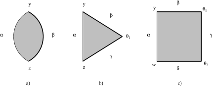
Figure 14. Holomorphic disks, triangles, and rectangles used to define a) $d({{{\bf y}}},{{{\bf z}}})$, b) $F_{\alpha,\beta,\gamma}({{{\bf y}}}\otimes\theta_{1})$, and c) ${\widehat{\mathcal{M}}}({{{\bf y}}},\theta_{1},\theta_{2},{{{\bf z}}})$. The heavy edges have sides parallel to $\beta_{g}$.

It follows that there are induced maps

$$\hat{F}^{i}_{\alpha,\beta,\gamma}(\cdot\otimes\theta_{1}) {{\colon}}{{\mathcal{S}}}_{2}^{i}({{\bf T}}_{\alpha},{{\bf T}}_{\beta})\to{{\mathcal{S}}}_{2}^{i}({{\bf T}}_{\alpha},{{\bf T}}_{\gamma})$$

$$\hat{F}^{i}_{\alpha,\gamma,\delta}(\cdot\otimes\theta_{2}) {{\colon}}{{\mathcal{S}}}_{2}^{i}({{\bf T}}_{\alpha},{{\bf T}}_{\gamma})\to{{\mathcal{S}}}_{2}^{i}({{\bf T}}_{\alpha},{{\bf T}}_{\delta})$$

$$\hat{F}^{i}_{\alpha,\beta,\delta}(\cdot\otimes\theta_{3}) {{\colon}}{{\mathcal{S}}}_{2}^{i}({{\bf T}}_{\alpha},{{\bf T}}_{\beta})\to{{\mathcal{S}}}_{2}^{i}({{\bf T}}_{\alpha},{{\bf T}}_{\delta})$$

Our next step is to check that associativity still holds:

Lemma 5.6.

$$\hat{F}^{i}_{\alpha,\gamma,\delta}(\hat{F}^{i}_{\alpha,\beta,\gamma}({{{\bf y}}}\otimes\theta_{1})\otimes\theta_{2})=\hat{F}^{i}_{\alpha,\beta,\delta}({{{\bf y}}}\otimes\hat{F}_{\beta,\gamma,\delta}(\theta_{1}\otimes\theta_{2}))$$

Proof.

We recall the proof of associativity in Lemma 5.11 of [19]. By examining the ends of an appropriate moduli space ${\widehat{\mathcal{M}}}({{{\bf y}}},\theta_{1},\theta_{2},{\bf w})$ of psuedoholomorphic rectangles, one sees that the statement of the lemma is false at the chain level, but that the error is given by

$$\sum_{{\bf w^{\prime}}\in{{\bf T}}_{\alpha}\cap{{\bf T}}_{\delta}}\#{\widehat{\mathcal{M}}}({{{\bf y}}},\theta_{1},\theta_{2},{\bf w^{\prime}})\cdot d({\bf w^{\prime}})$$

Since $d({\bf w^{\prime}})$ is exact, the statement is true at the level of homology.

The same argument will prove our version of the statement if we can show that for ${{{\bf y}}}\in{{\mathcal{S}}}^{i}_{1}({{\bf T}}_{\alpha},{{\bf T}}_{\beta})$, the error term is exact in ${{\mathcal{S}}}^{i}_{1}({{\bf T}}_{\alpha},{{\bf T}}_{\delta})$. To prove this, it suffices to check $\#{\widehat{\mathcal{M}}}({{{\bf y}}},\theta_{1},\theta_{2},{\bf w^{\prime}})=0$ whenever $A({\bf w^{\prime}})>A({{{\bf y}}})$. Referring to Figure 14c, we see that this follows from Lemma 5.4. ∎

Proposition 5.2.

${{\widehat{CF}_{r}}}(N,m,{{\mathbf{s}}})$ is invariant under $\beta$ handleslides in $N$ whose support is disjoint from ${{\mathfrak{m}}}$.

Proof.

If necessary, we slide and isotope $\beta_{g}$ so that it is disjoint from the support of the handleside in question. Since ${{\widehat{CF}_{s}}}({{\mathcal{H}}})\cong{{\widehat{CF}_{s}}}({{\mathcal{H}}},{{\overline{N}}})$, this has no effect on ${{\widehat{CF}_{s}}}({{\mathcal{H}}})$. Thus we may assume that the handleslide on our Heegaard splitting for $N$ extend to a handleslide on our splitting for $N(n,1)$.

We have a filtered chain map $\hat{f}_{\alpha,\beta,\gamma}:{{\widehat{CF}_{s}}}({{\bf T}}_{\alpha},{{\bf T}}_{\beta})\to{{\widehat{CF}_{s}}}({{\bf T}}_{\alpha},{{\bf T}}_{\gamma})$. To prove that the associated reduced map is an isomorphism, it suffices to show that the maps $\hat{F}^{i}_{\alpha,\beta,\gamma}:{{\mathcal{S}}}^{i}_{2}({{\bf T}}_{\alpha},{{\bf T}}_{\beta})\to{{\mathcal{S}}}^{i}_{2}({{\bf T}}_{\alpha},{{\bf T}}_{\gamma})$ are isomorphisms. This follows from the associativity relation proved in the previous lemma, the identity $\hat{F}_{\beta,\gamma,\delta}(\theta_{1}\otimes\theta_{2})=\theta_{3}$, and the fact (Lemma 5.12 of [19]) that $\hat{f}_{\alpha,\beta,\delta}:{{\widehat{CF}}}({{\bf T}}_{\alpha},{{\bf T}}_{\beta})\to{{\widehat{CF}}}({{\bf T}}_{\alpha},{{\bf T}}_{\delta})$ is a filtration preserving isomophism. ∎

Although this proof is more complex than our previous arguments involving filtered chain homotopies, it is similar in spirit. We still have a filtered chain map ${{\widehat{CF}_{s}}}({{\mathcal{H}}})\to{{\widehat{CF}_{s}}}({{\mathcal{H}}}^{\prime})$. The role of the chain homotopy is now played by the associativity relation, and the fact that the chain homotopy is filtered is replaced by the fact that the relevant holomorphic rectangles respect the Alexander filtration.

Next, suppose that we are sliding an $\alpha$ handle in the Heegaard splitting of $N$. We modify our labeling so that $\gamma$ is the set of $\alpha$ handles after the handleslide, and $\delta$ is a parallel copy of $\alpha$. There are chain maps

$$\hat{g}_{\alpha,\gamma,\beta}(\cdot\otimes\theta_{1}){{\colon}}\ {{\widehat{CF}}}({{\bf T}}_{\alpha},{{\bf T}}_{\beta})\to{{\widehat{CF}}}({{\bf T}}_{\gamma},{{\bf T}}_{\beta})$$

$$\hat{g}_{\gamma,\delta,\beta}(\cdot\otimes\theta_{2}){{\colon}}\ {{\widehat{CF}}}({{\bf T}}_{\gamma},{{\bf T}}_{\beta})\to{{\widehat{CF}}}({{\bf T}}_{\delta},{{\bf T}}_{\beta})$$

$$\hat{g}_{\alpha,\delta,\beta}(\cdot\otimes\theta_{3}){{\colon}}\ {{\widehat{CF}}}({{\bf T}}_{\alpha},{{\bf T}}_{\beta})\to{{\widehat{CF}}}({{\bf T}}_{\delta},{{\bf T}}_{\beta})$$

analogous to the $\hat{f}$’s. For example, $\hat{g}_{\alpha,\gamma,\beta}$ is defined by

$$\hat{g}_{\alpha,\gamma,\beta}({{{\bf y}}}\otimes\theta_{1})=\sum c({{{\bf y}}},{{{\bf z}}},\theta_{1})\cdot{{{\bf z}}}$$

where

$$c({{{\bf y}}},{{{\bf z}}},\theta_{1})=\sum_{\{\psi\in\pi_{2}({{{\bf y}}},{{{\bf z}}},\theta_{1}){{\thinspace}}|{{\thinspace}}\mu(\psi)=n_{z_{s}}(\psi)=0\}}\#{\widehat{\mathcal{M}}}(\psi).$$

(The easiest way to see this is the right definition is to reverse the orientation of $\Sigma$ and switch the roles of the $\alpha$ and $\beta$ handles. This leaves ${{\widehat{CF}_{s}}}({{\mathcal{H}}})$ unchanged, but now we are sliding “$\beta$” handles, so we can use the definitions of [19]. Translating back to our original setting, we arrive at the definition above.)

Proposition 5.3.

${{\widehat{CF}_{r}}}$ is invariant under the action of sliding one $\alpha$ handle over another.

Proof.

We argue as in the proof of Proposition 5.2. First, we need to check that the $\hat{g}$’s respect the Alexander filtration. The form of the triangles we count to define $\hat{g}_{\alpha,\gamma,\beta}$ is shown in Figure 15a. Since $\alpha$ and $\gamma$ do not have any sides parallel to the spiral handle $\beta_{g}$, Lemma 5.4 applies. It follows that $c({{{\bf y}}},{{{\bf z}}},\theta_{1})=0$ unless $A({{{\bf y}}})\geq A({{{\bf z}}})$, so $\hat{g}_{\alpha,\gamma,\beta}$ respects the Alexander filtration. Similar arguments apply to the other $\hat{g}$’s.

Next, we need to check that associativity holds, i.e. that

$$\hat{G}^{i}_{\gamma,\delta,\beta}(\hat{G}^{i}_{\alpha,\gamma,\beta}({{{\bf y}}}\otimes\theta_{1})\otimes\theta_{2})=\hat{G}^{i}_{\alpha,\delta,\beta}({{{\bf y}}}\otimes\hat{G}_{\alpha,\gamma,\delta}(\theta_{1}\otimes\theta_{2}))$$

For the unfiltered maps (without the $i$’s), this is proved in the usual way, by studying degenerations of the space of holomorphic rectangles of the sort illustrated in Figure 15b. As in Lemma 5.6, the statement is false at the chain level, but the error is

$$\sum_{{\bf w}^{\prime}\in{{\bf T}}_{\delta}\cap{{\bf T}}_{\beta}}\#{\widehat{\mathcal{M}}}({{{\bf y}}},{\bf w}^{\prime},\theta_{2},\theta_{1})d({\bf w}^{\prime})$$

Referring to the rectangle of Figure 15b, we see that Lemma 5.4 applies in this case as well, so $\#{\widehat{\mathcal{M}}}({{{\bf y}}},{\bf w}^{\prime},\theta_{2},\theta_{1})=0$ unless $A({{{\bf y}}})\geq A({\bf w}^{\prime})$. This proves the desired relation.

It is straightforward to check that the remaining elements of the proof of handleslide invariance — the fact that $\hat{G}_{\alpha,\gamma,\delta}(\theta_{1}\otimes\theta_{2})=\theta_{3}$ and that $\hat{g}_{\alpha,\delta,\beta}(\cdot\otimes\theta_{3})$ is an isomorphism at the chain level — extend to the $\alpha$ handleslide case. The result now follows by the same arguments as Proposition 5.2. ∎

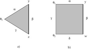
Figure 15. Holomorphic triangles and rectangles used to define a) $G_{\alpha,\gamma,\beta}({{{\bf y}}}\otimes\theta_{1})$ and b) ${\widehat{\mathcal{M}}}({{{\bf y}}},{\bf w},\theta_{2},\theta_{1})$. The heavy edges have a side parallel to $\beta_{g}$.

We can also use handleslides to modify ${{\mathfrak{m}}}$. Indeed, it is not difficult to see that the curve $m^{\prime}$ obtained by sliding ${{\mathfrak{m}}}$ over any one of the $\beta$ handles in the Heegaard splitting of $N$ is another geometric representative of the meridian. We would like to show that ${{\widehat{CF}_{r}}}$ is invariant under the operation of replacing ${{\mathfrak{m}}}$ by ${{\mathfrak{m}}}^{\prime}$. A priori, this situation seems to be more complicated than the previous ones, since the corresponding move in the closed manifold $N(n,1)$ is not a handleslide. Fortunately, Lemma 4.2 tells us that ${{\widehat{CF}_{s}}}({{\mathcal{H}}},{{\mathbf{s}}})\cong{{\widehat{CF}_{s}}}({{\mathcal{H}}},{{\overline{N}}},{{\overline{{{\mathbf{s}}}}}})$ as a filtered complex. Thus we can study the situation in ${{\overline{N}}}$, where sliding ${{\mathfrak{m}}}$ is an honest handleslide, albeit one involving the special handle.

Proposition 5.4.

${{\widehat{CF}_{r}}}$ is invariant under the operation of sliding ${{\mathfrak{m}}}$ over one of the $\beta_{i}$’s, so long as the slide is supported away from $z_{s}$.

Proof.

Let ${{\overline{{{\bf T}}}}}_{\beta},{{\overline{{{\bf T}}}}}_{\gamma}$ and ${{\overline{{{\bf T}}}}}_{\delta}$ be the tori in $s^{g}\Sigma$ induced by the $\beta$, $\gamma$ and $\delta$ handles in the Heegaard splittings for ${{\overline{N}}}$. (We revert to our original notation in which $\gamma$ and $\delta$ are derived from $\beta$.) As usual, there are maps

$$\hat{f}_{\alpha,\beta,\gamma}(\cdot\otimes\theta_{1}){{\colon}}\ {{\widehat{CF}}}({{\bf T}}_{\alpha},{{\overline{{{\bf T}}}}}_{\beta})\to{{\widehat{CF}}}({{\bf T}}_{\alpha},{{\overline{{{\bf T}}}}}_{\gamma})$$

$$\hat{f}_{\alpha,\gamma,\delta}(\cdot\otimes\theta_{2}){{\colon}}\ {{\widehat{CF}}}({{\bf T}}_{\alpha},{{\overline{{{\bf T}}}}}_{\gamma})\to{{\widehat{CF}}}({{\bf T}}_{\alpha},{{\overline{{{\bf T}}}}}_{\delta})$$

$$\hat{f}_{\alpha,\beta,\delta}(\cdot\otimes\theta_{3}){{\colon}}\ {{\widehat{CF}}}({{\bf T}}_{\alpha},{{\overline{{{\bf T}}}}}_{\beta})\to{{\widehat{CF}}}({{\bf T}}_{\alpha},{{\overline{{{\bf T}}}}}_{\delta})$$

which induce isomorphisms on ${{\widehat{HF}}}$.

Although there is no longer a spiral handle, it still makes sense to talk about the Alexander grading on ${{\widehat{CF}_{s}}}({{\mathcal{H}}},{{\overline{N}}})$ — it is defined by the relation $A({{\overline{\bf y}}})-A({{\overline{\bf y}}})=n_{z_{s}}(\phi)-n_{z_{a}}(\phi)$ for $\phi\in\pi_{2}({{\overline{\bf y}}},{{\overline{\bf z}}})$.

We would like to show that the $\hat{f}$’s respect the Alexander filtration. To do this, observe that for every ${{\overline{\bf y}}}\in{{\bf T}}_{\alpha}\cap{{\overline{{{\bf T}}}}}_{\beta}$ there is a “close” point ${{\overline{\bf y}}}^{\prime}\in{{\bf T}}_{\alpha}\cap{{\overline{{{\bf T}}}}}_{\gamma}$. Suppose ${{\overline{\bf y}}}\in{{\bf T}}_{\alpha}\cap{{\overline{{{\bf T}}}}}_{\beta}$ and ${{\overline{\bf z}}}\in{{\bf T}}_{\alpha}\cap{{\overline{{{\bf T}}}}}_{\gamma}$. Then to any $\psi\in\pi_{2}({{\overline{\bf y}}},\theta_{1},{{\overline{\bf z}}})$, there is associated a disk $\psi^{\prime}\in\pi_{2}({{\overline{\bf y}}}^{\prime},{{\overline{\bf z}}})$. To define $\psi^{\prime}$, we superimpose the $\beta$ and $\gamma$ handles, so they are indistinguishable except in the neighborhood of the handleslide shown in Figure 16. Then $\partial{{\mathcal{D}}}(\psi^{\prime})$ looks just like $\partial{{\mathcal{D}}}(\psi)$, except that every time the segment $B$ appears in $\partial{{\mathcal{D}}}(\psi)$, we replace it with the segment labeled $C$ together with an entire copy of $\gamma_{2}$. Since $C\cup\gamma_{2}$ is homologous to $B$, the multiplicities of ${{\mathcal{D}}}(\psi)$ and ${{\mathcal{D}}}(\psi^{\prime})$ agree outside of the shaded region in the figure.

By hypothesis the handleslide was supported away from $z$, so $n_{z_{a}}(\psi^{\prime})=n_{z_{a}}(\psi)$. Thus for ${{\mathcal{D}}}(\psi)$ to be positive, we must have $A({{{\bf y}}}^{\prime})-A({{{\bf z}}})=n_{z_{a}}(\psi^{\prime})\geq 0$. Thus ${{\hat{f}}}_{\alpha,\beta,\gamma}$ is a filtered map. Similar arguments (always comparing triangles with differentials in ${{\widehat{CF}}}({{\bf T}}_{\alpha}\cap{{\overline{{{\bf T}}}}}_{\gamma})$) show that the other $\hat{f}$’s are filtered and that the associativity relation holds. The proof then proceeds along the lines of Proposition 5.2.

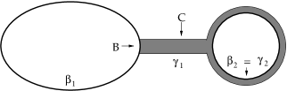
Figure 16. Comparison of the domains of $\psi$ and $\psi^{\prime}$.

∎

5.5. Stabilization invariance

Lemma 5.7.

${{\widehat{CF}_{r}}}$ is invariant under stabilization of the Heegaard splitting of $N$.

Proof.

Let ${{\widehat{CF}_{r}}}({{\mathcal{H}}}^{\prime})$ be the reduced complex for the stabilized Heegaard splitting. We claim that ${{\widehat{CF}_{r}}}({{\mathcal{H}}}^{\prime})$ is independent of the point $\sigma\in\Sigma-\alpha-\beta$ at which we stabilized. Indeed, stabilizing at another point $\sigma^{\prime}$ is the same as stabilizing at $\sigma$ followed by a sequence of handleslides. By Propositions 5.2 and 5.3, we know that ${{\widehat{CF}_{r}}}$ does not change under handleslide.

Thus we may as well assume that $\sigma$ is in the same component of $\Sigma-\alpha-{{\overline{\beta}}}$ as the point $z_{s}$. In this case, we are in the situation of Theorem 6.1 of [19], which proves that ${{\widehat{HF}}}$ is invariant under stabilization by showing that ${{\widehat{CF}_{s}}}({{\mathcal{H}}})$ and ${{\widehat{CF}_{s}}}({{\mathcal{H}}}^{\prime})$ are identical. Combined with the obvious fact that the Alexander grading on ${{\widehat{CF}_{s}}}({{\mathcal{H}}}^{\prime})$ is the same as the Alexander grading on ${{\widehat{CF}_{s}}}({{\mathcal{H}}})$, this proves the proposition.

∎

5.6. Invariance under change of basepoint

The situation with regard to our choice of basepoint is rather different than for ${{\widehat{HF}}}$. In the latter case, any basepoint will do, but in order to define ${{\widehat{CF}_{s}}}$, we required $z_{s}$ to be adjacent to ${{\mathfrak{m}}}$ and on the stable side (as defined by our choice of longitude back in section 3.5.) Thus the only real way that we can vary $z_{s}$ is to move it over one of the $w_{i}$’s.

Lemma 5.8.

${{\widehat{CF}_{r}}}(N)$ does not change if we move $z_{s}$ over one of the segments $w^{i}$.

Proof.

This is immediate from the proof that ${{\widehat{HF}}}$ is invariant under change of basepoint given Theorem 5.15 of [19]. Indeed, the argument there is based on the observation that we can obtain the effect of moving $z$ over $\alpha_{i}$ by a series of isotopies and handleslides of $\alpha_{i}$ supported away from $z$. But we know from Propositions 5.1 and 5.3 that ${{\widehat{CF}_{r}}}$ is invariant under these moves. ∎

Note that it is usually not true that the complex ${{\widehat{CF}_{r}}}(N,m,{{\mathbf{s}}})$ is the same as the complex ${{\widehat{CF}_{r}}}^{a}(N,m,{{\mathbf{s}}})$ that we get by moving the basepoint to the other side of $m$; this is only the case when ${{\mathbf{s}}}={{\overline{{{\mathbf{s}}}}}}$. This is the reason we required $z_{s}$ to be on the side corresponding to positive ${{\mathrm{Spin}^{c}}}$ structures.

5.7. Conclusion of proof

To wrap things up, we need a pair of geometric lemmas.

Lemma 5.9.

Let $N$ be a knot complement in a general three-manifold. Any two Heegaard splittings of $N$ differ by a sequence of isotopies, handleslides, stabilizations, and destabilizations.

This is proved in the same way as the closed case.

Lemma 5.10.

For a fixed Heegaard splitting of $N$, any two geometric representatives of $m$ are connected by a series of isotopies and handleslides over the $\beta_{i}$’s.

Proof.

Recall that $\partial N$ is obtained by surgering $\Sigma$ along $\beta_{1},\beta_{2},\ldots\beta_{g-1}$. Thus we can think of $\partial N$ as a torus with $2g-2$ small marked disks (the surgery disks) on it. Any two geometric representatives of ${{\mathfrak{m}}}$ are connected by an isotopy on this torus, and it is easy to see that this isotopy extends to $\Sigma$ except when ${{\mathfrak{m}}}$ crosses over one of the marked disks. At these points, ${{\mathfrak{m}}}$ slides over the corresponding $\beta_{i}$ on $\Sigma$. ∎

We now prove of Theorem 4. Suppose we have two Heegaard splittings $(\Sigma,\alpha,\beta)$ and $(\Sigma^{\prime},\alpha^{\prime},\beta^{\prime})$ with meridians ${{\mathfrak{m}}}$ and ${{\mathfrak{m}}}^{\prime}$ and basepoints $z_{s}$ and $z_{s}^{\prime}$. We start by transforming the first Heegaard splitting into the second by a sequence of isotopies, handleslides, stabilizations, and destabilizations. We have already checked that these moves preserve ${{\widehat{CF}_{r}}}$. As we make these moves, however, we may also have to change our choice of $z_{s}$ and ${{\mathfrak{m}}}$, since we may have isotoped an $\alpha$ handle over $z_{s}$ or a $\beta$ handle over ${{\mathfrak{m}}}$. In the former case, we use Lemma 5.8 to see that we can move $z_{s}$ over the $\alpha$ handle without changing ${{\widehat{CF}_{r}}}$. In the latter, we isotope and slide ${{\mathfrak{m}}}$ to keep it from intersecting any of the $\beta$ handles. Propositions 5.1 and 5.4 ensure that ${{\widehat{CF}_{r}}}$ is invariant under these moves as well. As we isotope ${{\mathfrak{m}}}$, we move $z_{s}$ along with it, so that it is always adjacent to ${{\mathfrak{m}}}$. The only situation in which it is not possible to do this is shown in Figure 17. In this case, the problem is rectified simply by moving $z_{s}$ over $\alpha_{i}$ before doing the isotopy.

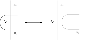
Figure 17. To do this isotopy, first move $z_{s}$ over $\alpha_{i}$.

Once we have turned $(\Sigma,\alpha,\beta)$ , into $(\Sigma^{\prime},\alpha^{\prime},\beta^{\prime})$ we isotope and slide the resulting ${{\mathfrak{m}}}$ until it is the same as ${{\mathfrak{m}}}^{\prime}$. (In doing so, we may need to move $z_{s}$ over some more $\alpha$ handles.) We have thus transformed our first diagram into a diagram which is identical to our second diagram except for the position of the basepoint. Since $z_{s}$ is by definition on the side of ${{\mathfrak{m}}}$ corresponding to the positive ${{\mathrm{Spin}^{c}}}$ structures, the resulting $z_{s}$ is on the same side of ${{\mathfrak{m}}}$ as $z_{s}^{\prime}$. Thus we can move $z_{s}$ over $\alpha$ handles until it is in same position as $z_{s}^{\prime}$. This concludes the proof.

6. Perfect Knots

Up to this point, we have considered the Ozsváth-Szabó  Floer homology from a purely theoretical standpoint. We now describe a case in which we can actually compute the groups in question.

Definition 6.1.

Let $K$ be a knot in $S^{3}$. We say that $K$ is perfect if the homological and Alexander gradings on ${{\widehat{CF}_{r}}}(K)$ are the same.

If $K$ is perfect, the rank of ${{\widehat{CF}_{r}}}^{(j)}(K)$ is equal to the absolute value of the coefficient of $t^{j}$ in $\Delta_{K}(t)$. Perfection is thus a very strong condition on $K$. Despite this fact, it is satisfied by a surprisingly large number of knots. In [25], we showed that two-bridge knots are perfect and described how to compute their Ozsváth-Szabó  Floer homology. In fact, the arguments of that paper apply equally well to any perfect knot. This fact was alluded to in [25], but with a more restrictive definition of “perfect,” which required the Alexander and homological gradings to agree on ${{\widehat{CF}_{s}}}(E)$. We will show in section 8 that the new definition is a substantial improvement: there are many knots whose stable complexes are not perfect, but whose reduced stable complexes are.

In this section, we repeat the calculation of [25], both for the sake of completeness and because our improved understanding of the Alexander filtration enables us to give a (hopefully) cleaner exposition. We conclude by showing that the the class of perfect knots is closed under connected sum.

6.1. Preliminaries

We fix some basic conventions regarding perfect knots. As usual, we choose a Heegaard splitting $(\Sigma,\alpha,\beta)$ for ${{K^{o}}}$, twist up, and choose some good $\epsilon$-class $E$. From the discussion in section 4.6, we know that ${{CF^{+}}}({{\mathcal{H}}},{{\mathbf{s}}}_{k})$ is chain homotopy equivalent to a reduced complex, which we denote by ${{CF_{r}^{+}}}(K,{{\mathbf{s}}}_{k})$. (Although we have dropped the reference to ${{\mathcal{H}}}$, we do not need to know that ${{CF_{r}^{+}}}(K,{{\mathbf{s}}}_{k})$ is canonical in what follows — just that it exists.)

Lemma 6.1.

If $K$ is perfect, the Alexander and homological gradings on ${{CF_{r}^{+}}}(K,{{\mathbf{s}}}_{k})$ are the same.

Proof.

The generators of ${{CF_{r}^{+}}}(K,{{\mathbf{s}}}_{k})$ are of the form $[{{{\bf y}}},i]$, where ${{{\bf y}}}$ is a generator of ${{\widehat{CF}_{r}}}(K)$. By definition, $A([{{{\bf y}}},i])=A({{{\bf y}}})+2i$ and ${{\mathrm{gr}}}([{{{\bf y}}},i])={{\mathrm{gr}}}({{{\bf y}}})+2i$. Since $K$ is perfect, $A({{{\bf y}}})={{\mathrm{gr}}}({{{\bf y}}})$. ∎

It is often convenient to think of the complexes ${{CF_{r}^{+}}}(K,{{\mathbf{s}}}_{k})$ as “dot stacks” like the one shown in Figure 10. Recall that each dot represents a collection of generators, all with the same Alexander gradings. By the lemma, the vertical axis of such a figure represents not only the Alexander grading on ${{CF_{r}^{+}}}(K,{{\mathbf{s}}}_{k})$, but also the homological grading. Since the two are the same, we often just refer to the grading of a generator in ${{CF_{r}^{+}}}(K,{{\mathbf{s}}}_{k})$, without specifying which one we are talking about.

Lemma 6.2.

${{HF_{s}^{+}}}(K)\cong{{{\bf{Z}}[u^{-1}]}}$ where $1\in{{{\bf{Z}}[u^{-1}]}}$ has grading $s(K)$. Similarly ${{HF_{s}^{-}}}(K)\cong{\bf{Z}}[u]$, where $1\in{\bf{Z}}[u]$ has grading $s(K)-2$.

Proof.

Since $K$ is a knot in $S^{3}$, ${{\widehat{HF}_{s}}}(K)\cong{\bf{Z}}$. The generator has grading $s(K)$ by definition. The obvious filtration on ${{CF_{s}^{+}}}(K)$ gives a spectral sequence with $E_{2}$ term ${{\widehat{HF}_{s}}}(E)\otimes{{{\bf{Z}}[u^{-1}]}}$ converging to ${{CF_{s}^{+}}}(K)$. Since ${{\widehat{HF}_{s}}}(K)\cong{\bf{Z}}$, the sequence collapses at the $E_{2}$ term. The result for ${{HF_{s}^{-}}}(K)$ follows from the analogous spectral sequence. ∎

In what follows, we will often consider the operation of truncating a chain complex $C$ above level $k$. The truncated complex is just the quotient complex $C_{\geq k}$ consisting of all elements of $C$ with homological grading $\geq k$. It is clear that $H_{*}(C_{\geq k})$ is trivial for $*<k$, is isomorphic to $H_{*}(C)$ for $*>k$, and has $H_{k}(C)$ as a subgroup for $*=k$. Similar results hold for the subcomplex $C_{\leq k}$ obtained by truncating $C$ below level $k$.

6.2. Computing $H_{*}(C_{{{\mathbf{s}}}_{k}}(K))$

Recall from Corollary 4.2 that we have a short exact sequence

$$\begin{CD}0@>{}>{}>C_{{{\mathbf{s}}}_{k}}@>{}>{}>{{CF_{r}^{+}}}(K,{{\mathbf{s}}}_{k})@>{}>{}>{{CF_{r}^{+}}}(K,{{\mathbf{s}}}_{s})@>{}>{}>0\end{CD}$$

where $C_{{{\mathbf{s}}}_{k}}$ is the subcomplex depicted in Figure 18.

Figure 18. a) the subcomplex $C_{{{\mathbf{s}}}_{k}}(K)$, compared with b) ${{CF_{a}^{+}}}(K)$ and c) ${{CF_{s}^{-}}}(K)$.

We will compute $H_{*}(C_{{{\mathbf{s}}}_{k}}(K))$ and then use the long exact sequence on homology to find ${{CF_{r}^{+}}}(K,{{\mathbf{s}}}_{k})$. Since ${{HF^{+}}}(K,{{\mathbf{s}}}_{k})\cong{{HF^{+}}}(K,{{\mathbf{s}}}_{-k})$, we may as well assume $k\geq 0$.

We denote the ${\bf{Z}}[u]$ module ${\bf{Z}}[u]/(u^{n})$ by ${{\mathcal{T}}}_{n}$.

Proposition 6.1.

For $k\geq 0$,

$$H_{*}(C_{{{\mathbf{s}}}_{k}}(K))\cong{{\mathcal{T}}}_{n_{k}}\oplus{\bf{Z}}^{m_{k}}$$

where

$$n_{k} =\max(\lceil(|s(K)|-k)/2\rceil,0)$$

$$m_{k} =\chi(C_{{{\mathbf{s}}}_{k}}(K))-(-1)^{s(K)-k}n_{k}$$

$$=\sum_{i>k}(i-k)a_{i}-(-1)^{s(K)-k}n_{k}$$

where $a^{i}$ is the coefficient of $t^{i}$ in $\Delta_{K}(t)$. The grading of the ${\bf{Z}}^{m_{k}}$ summand is always $k-1$. The grading of $1\in{{\mathcal{T}}}_{n_{k}}$ is $s(K)-2$ if $s(K)>0$ and either $k-1$ (if $k\equiv s(K)\mod 2$ ) or $k-2$ (if $k\not\equiv s(K)\mod 2$) when $s(K)<0$.

Less formally, $H_{*}(C_{{{\mathbf{s}}}_{k}}(K))$ is composed of two parts. The first part is concentrated in grading $k-1$ and has trivial $u$ action, and the second is a torsion module generated by a single element. If $s(K)>0$, this module starts at level $s(K)$ and stretches down to level $k-1$ (or just above it), while if $s(K)<0$ it starts at or just below $k-1$ and extends downward. If $n_{k}\geq s(K)$, the torsion module is empty. Note that $\chi(C_{{{\mathbf{s}}}_{k}}(K))=\chi({{HF^{+}}}(K(0,1),{{\mathbf{s}}}_{k}))$. In fact, in [18], Ozsváth and Szabó compute the right-hand Euler characteristic by showing it is equal to the left-hand one.

Proof.

Observe from Figure 18 that if we truncate $C_{{{\mathbf{s}}}_{k}}(K)$ above level $k-1$, we get same complex that we do by truncating ${{CF_{s}^{-}}}(K)$ above level $k-1$. Similarly, if we truncate $C_{{{\mathbf{s}}}_{k}}(K)$ below level $k-1$, we get a complex which is isomorphic to ${{CF_{a}^{-}}}(K)$ truncated at level $-k-1$. It follows that

$$H_{*}(C_{{{\mathbf{s}}}_{k}}(K))\cong\begin{cases}{{HF_{s}^{-}}}_{*}(K)&\text{if}\ *>k-1\\ {{HF_{a}^{+}}}_{*-2k}(K)&\text{if}\ *<k-1.\end{cases}$$

For $*\neq k-1$, the claim now follows from Lemma 6.2 and the isomorphism ${{HF_{a}^{+}}}(K)\cong{{HF_{s}^{+}}}(K)$. Note that our assumption that $k\geq 0$ ensures that one of ${{HF_{a}^{+}}}(K)$ or ${{HF_{s}^{-}}}(K)$ must be trivial over the range in question.

Since we know the rank of $H_{*}(C_{{{\mathbf{s}}}_{k}}(K))$ for $*\neq k$, we can use $\chi(C_{{{\mathbf{s}}}_{k}}(K))$ to compute the rank of $H_{k-1}(C_{{{\mathbf{s}}}_{k}}(K))$. To see this group is torsion free, we note that the argument given above also applies if we use coefficients in ${\bf{Z}}/p$. Since $H_{*}(C_{{{\mathbf{s}}}_{k}}(K);{\bf{Z}}/p)\cong H_{*}(C_{{{\mathbf{s}}}_{k}}(K))\otimes{\bf{Z}}/p$ for $*\neq k-1$, the universal coefficient theorem implies that $H_{k-1}(C_{{{\mathbf{s}}}_{k}}(K))$ is free.

To finish the proof, we need only check that the ${\bf{Z}}[u]$ module structure is as described. If ${{\mathcal{T}}}_{n_{k}}$ and ${\bf{Z}}^{m_{k}}$ have different parities, this is obvious from the grading. If they have the same parity, we must show, e.g that if $s(K)>0$ and $n_{k}>1$, then $H_{k-1}(C_{{{\mathbf{s}}}_{k}}(K))$ contains an element in the image of $u$. But this is obvious, since $H_{k-1}(C_{{{\mathbf{s}}}_{k}}(K))$ contains $({{HF_{s}^{-}}})_{k-1}(K)$ as a submodule, and the (unique) generator of the latter group is in the image of $u$. The case when $s(K)<0$ is similar. ∎

6.3. Computing ${{HF^{+}}}(K,{{\mathbf{s}}}_{k})$

We have a long exact sequence of ${\bf{Z}}[u]$ modules

$$\begin{CD}@>{}>{}>H_{*}(C_{{{\mathbf{s}}}_{k}}(K))@>{}>{}>{{HF^{+}}}_{*}(K,{{\mathbf{s}}}_{k})@>{g}>{}>{{HF_{s}^{+}}}_{*}(K)@>{}>{}>\end{CD}$$

Since ${{CF_{r}^{+}}}(K,{{\mathbf{s}}}_{k})$ is identical to ${{CF_{r}^{+}}}(K,{{\mathbf{s}}}_{s})$ when the grading is large enough, ${{HF^{+}}}(K,{{\mathbf{s}}}_{k})$ has a ${{{\bf{Z}}[u^{-1}]}}$ summand $A$ which maps onto ${{CF_{r}^{+}}}(K,{{\mathbf{s}}}_{s})\cong{{{\bf{Z}}[u^{-1}]}}$. Thus the long exact sequence reduces to a short exact sequence

$$\begin{CD}0@>{}>{}>H_{*}(C_{{{\mathbf{s}}}_{k}}(K))@>{}>{}>{{HF^{+}}}_{*}(K,{{\mathbf{s}}}_{k})@>{g}>{}>{{{\bf{Z}}[u^{-1}]}}@>{}>{}>0\end{CD}$$

from which we can easily compute ${{HF^{+}}}_{*}(K,{{\mathbf{s}}}_{k})$.

Theorem 6.1.

For $k\geq 0$,

$${{HF^{+}}}(K,{{\mathbf{s}}}_{k})\cong\begin{cases}{\bf{Z}}^{m_{k}}\oplus{{{\bf{Z}}[u^{-1}]}}&\text{if}\ s(K)\geq 0\\ H_{*}(C_{{{\mathbf{s}}}_{k}}(K))\oplus{{{\bf{Z}}[u^{-1}]}}&\text{if}\ s(K)\leq 0\end{cases}$$

If $s(K)\geq 0$, the grading of $1\in{{{\bf{Z}}[u^{-1}]}}$ is $s(K)-2n_{k}$, while if $s(K)\leq 0$ it is $s(K)$.

Proof.

When viewed as abelian group, ${{HF^{+}}}(K,{{\mathbf{s}}}_{k})$ decomposes as $H_{*}(C_{{{\mathbf{s}}}_{k}}(K))\oplus{{HF_{s}^{+}}}(K)$, but this does not necessarily hold when we view it as a ${\bf{Z}}[u]$ module. What we do know is that $H_{*}(C_{{{\mathbf{s}}}_{k}},(K))\cong A\oplus B$, where $A\cong{{{\bf{Z}}[u^{-1}]}}$ and $B$ is a finitely generated torsion module. $A$ maps onto ${{HF_{s}^{+}}}(K)$, but the map may have some kernel. To determine if this is the case, we rely on the grading. By Lemma 6.2, the grading of $1\in{{HF_{s}^{+}}}(K)\cong{{{\bf{Z}}[u^{-1}]}}$ is $s(K)$. We now analyze the cases $s(K)\geq 0$ and $s(K)\leq 0$ separately.

Suppose first that $s(K)\leq 0$. In this case, the lowest grading attained by any element of $H_{*}(C_{{{\mathbf{s}}}_{k}}(K))$ is $k-1$ if $n_{k}$ = 0, and either $k-2n_{k}$ or $k+1-2n_{k}$ if $n_{k}>0$. In particular, this lowest grading is always greater than or equal to $s(K)-1$. It follows that the grading of $1\in A$ cannot be less than $s(K)$. (It is congruent to $s(K)\mod 2$.) Thus it must be equal to $s(K)$, and the map $A\to{{HF_{s}^{+}}}(K)$ is an isomorphism. It follows that the short exact sequence splits as a sequence of ${{{\bf{Z}}[u^{-1}]}}$ modules. This proves the theorem when $s(K)\leq 0$.

When $s(K)\geq 0$, we consider two subcases. If $k\geq s(K)$, $n_{k}=0$, and all the elements of $H_{*}(C_{{{\mathbf{s}}}_{k}}(K))$ have grading $k-1$. Since this is greater than or equal to $s(K)-1$, the same argument shows that the exact sequence splits. On the other hand, when $k<s(K)$, we claim that the grading of $1\in A$ is either $k$ or $k-1$ (depending on the parity of $k$.) To see this, we refer back to Figure 18 and observe that if we truncate ${{CF_{r}^{+}}}(K,{{\mathbf{s}}}_{k})$ above level $k$, we get ${{CF^{\infty}}}(K)_{\geq k}$. Since ${{HF^{\infty}}}(K)\cong{\bf{Z}}[u,u^{-1}]$, ${{HF^{+}}}(K,{{\mathbf{s}}}_{k})$ contains a ${{{\bf{Z}}[u^{-1}]}}$ summand with an element of grading either $k$ or $k-1$. The grading of every element in ${{HF^{+}}}(K,{{\mathbf{s}}}_{k})$ is at least $k-1$, so the claim is true. Thus the ${{\mathcal{T}}}_{n_{k}}$ summand of $H_{*}(C_{{{\mathbf{s}}}_{k}}(K))$ is the kernel of the map $A\to{{{\bf{Z}}[u^{-1}]}}$, and ${{HF^{+}}}(K,{{\mathbf{s}}}_{k})\cong{\bf{Z}}^{m_{k}}\oplus{{{\bf{Z}}[u^{-1}]}}$. ∎

Remark: The method of computation employed here is not strictly limited to perfect knots. There exist knots which are not perfect, but which still have the property that $C_{k}$ looks like ${{CF_{s}^{-}}}(K)$ when truncated above some level $l$ , and like ${{CF_{a}^{+}}}(K)$ when truncated below $l$. The argument above can be easily modified to compute ${{HF^{+}}}(K,{{\mathbf{s}}}_{k})$ in such cases. Examples of such knots include the torus knots and the knot $10_{139}$.

6.4. $s(K)$ and $\sigma(K)$

Theorem 6.1 can be interpreted as saying that for a perfect knot $K$, the groups ${{HF^{+}}}(K,{{\mathbf{s}}}_{k})$ are completely determined by the Alexander polynomial of $K$ and the invariant $s(K)$. For all perfect knots we are aware of, $s(K)$ is determined by the classical knot signature: $s(K)=\sigma(K)/2$. In fact, Ozsváth and Szabó have proved in [22] that this equality holds for all alternating knots.

It would be nice to have a geometrical explanation for this phenomenon. One way to look at the matter is to say that for small perfect knots, $s(K)$ and $\sigma(K)$ are determined by the same set of skein theoretic axioms. If $L$ is an oriented link in $S^{3}$, we can inductively construct a skein resolution tree $T(L)$ for $L$ as follows. If $L$ is the unlink, $T(L)={L}$. If $L$ is not the unlink, pick a crossing of $L$, and let $L_{0}$ and $L^{\prime}$ be the links obtained by resolving the crossing in an oriented fashion and changing the crossing. (Of course, such trees are not unique.) Given a skein tree for a knot $K$, we can use the skein relation to inductively compute $\Delta_{K}(t)$. It is also possible to compute $\sigma(K)$ from a skein tree. (See, e.g [7], p. 207.)

Now suppose that $L$, $L^{\prime}$ and $L_{0}$ are all perfect, and that two of the three have $s=\sigma/2$. Then using the skein exact triangle, it is possible to show that the same relation holds for the third. Thus if $K$ has a skein resolution tree all of whose elements are perfect, it is necessarily the case that $s(K)=\sigma(K)/2$. All the perfect knots we are aware of have such perfect resolutions. It is an interesting question whether all perfect knots have perfect resolutions, and, more generally, whether all perfect knots satisfy $s(K)=\sigma(K)/2$.

6.5. Connected Sums

Let $K_{i}\subset{{\overline{N}}}_{i}$ ($i=1,2$) be knots, and consider their connected sum $K_{1}\#K_{2}\subset{{\overline{N}}}_{1}\#{{\overline{N}}}_{2}$. The complement of $K_{1}\#K_{2}$ is obtained from the $N_{i}$ by taking a boundary connected sum along the $m_{i}$. To be precise, we identify a tubular neighborhood of $m_{1}\subset\partial N_{1}$ with a tubular neighborhood of $m_{2}\subset\partial N_{2}$ to produce a new manifold $N_{1}\#_{m}N_{2}$ which is the complement of $K_{1}\#K_{2}$. The reduced stable complex behaves nicely with respect to this operation:

Proposition 6.2.

$${{\widehat{CF}_{r}}}(N_{1}\#_{m}N_{2},m)\cong{{\widehat{CF}_{r}}}(N_{1},m_{1})\otimes{{\widehat{CF}_{r}}}(N_{2},m_{2}).$$

Specializing to the case of knots in $S^{3}$, we get

Corollary 6.1.

The connected sum of two perfect knots is perfect.

Corollary 6.2.

If $K_{1}$ and $K_{2}$ are knots in $S^{3}$, then $s(K_{1}\#K_{2})=s(K_{1})+s(K_{2})$.

Figure 19. Heegaard splittings of $N_{1}$, $N_{2}$, and ${{N_{1}\#_{m}N_{2}}}$.

The remainder of this section is devoted to the proof of the proposition. First, we explain how to get a Heegaard splitting of ${{N_{1}\#_{m}N_{2}}}$ from splittings of $N_{1}$ and $N_{2}$. By Lemma 3.4, we can choose a Heegaard splitting ${{\mathcal{H}}}_{1}=(\Sigma^{1},\alpha^{1},\beta^{1})$ of $N_{1}$ with the property that $m_{1}$ has a geometric representative which intersects $\alpha_{1}^{1}$ geometrically once and misses all the other $\alpha^{1}_{i}$’s. Such a splitting is shown schematically in Figure 19. If we choose a splitting ${{\mathcal{H}}}_{2}=(\Sigma^{2},\alpha^{2},\beta^{2})$ of $N_{2}$ with the same property, then we can “sum the Heegaard splittings” along $\alpha_{1}^{1}$ and $\alpha_{1}^{2}$ to obtain a splitting ${{\mathcal{H}}}=(\Sigma,\alpha,\beta)$ of ${{N_{1}\#_{m}N_{2}}}$, as indicated in Figure 19. To be precise, $\Sigma$ is obtained by cutting $\Sigma^{i}$ open along $m_{i}$ and then gluing $\Sigma^{1}$ to $\Sigma^{2}$ along the two resulting circles. It has genus $g_{1}+g_{2}-1$. On $\Sigma$, we join $\alpha_{1}^{1}$ and $\alpha_{1}^{2}$ (which have been cut open) into a single large attaching circle $\alpha_{1}$. All the other attaching circles are disjoint from the $m_{i}$ and remain unchanged.

To see why this procedure works, consider the $\alpha$ handlebodies inside $N_{1}$ and $N_{2}$. The meridians are circles on the boundaries of these handlebodies, and by hypothesis there is a system of compressing disks so that only one disk intersects each meridian. To take the boundary connect sum along the meridians, we sandwich the two handlebodies together, as in Figure 20. The result is a new handlebody, with $\alpha_{1}$ in place of $\alpha_{1}^{1}$ and $\alpha_{1}^{2}$. The other attaching circles are unaffected.

From this description, it is easy to see that $\overline{N_{1}\#_{m}N_{2}}={{\overline{N}}}_{1}\#{{\overline{N}}}_{2}$. Indeed, if we attach a final handle along ${{\mathfrak{m}}}$, we can cancel it with $\alpha_{1}$ to obtain a diagram which is the connected sum of diagrams for $N_{1}$ and $N_{2}$. As a consequence, a ${{\mathrm{Spin}^{c}}}$ structure on $N_{1}\#_{m}N_{2}$ is naturally identified with a pair of ${{\mathrm{Spin}^{c}}}$ structures on $N_{1}$ and $N_{2}$.

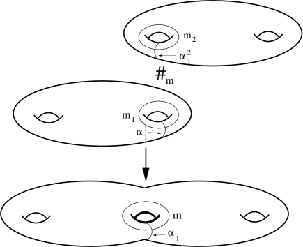
Figure 20. Another view of $N_{1}\#_{m}N_{2}$.

Fix ${{\mathrm{Spin}^{c}}}$ structures ${{\mathbf{s}}}_{i}$ on $N_{i}$, and let $E_{i}$ be a good $\epsilon$-class for $({{\mathcal{H}}}_{i},{{\mathbf{s}}}_{i})$. Since ${{\mathfrak{m}}}_{1}$ has only a single intersection with $\alpha_{1}^{1}$, the elements of $E_{1}$ are in $1-1$ correspondence with elements of ${{\bf T}}_{\hat{\alpha}_{1}^{1}}\cap{{\bf T}}_{\hat{\beta}^{1}}$, and similarly for $E_{2}$. Likewise, ${{\mathfrak{m}}}$ has a unique intersection with $\alpha_{1}$, so the elements in a good $\epsilon$-class $E$ for $({{\mathcal{H}}},{{\mathbf{s}}}_{1}\#{{\mathbf{s}}}_{2})$ correspond to elements of

$${{\bf T}}_{\hat{\alpha}_{1}}\cap{{\bf T}}_{\hat{\beta}}\cong({{\bf T}}_{\hat{\alpha}_{1}^{1}}\cap{{\bf T}}_{\hat{\beta}^{1}})\times({{\bf T}}_{\hat{\alpha}_{1}^{2}}\cap{{\bf T}}_{\hat{\beta}^{2}}).$$

Thus $E$ is naturally identified with $E_{1}\times E_{2}$.

To define the Alexander grading, we orient ${{\mathfrak{m}}}_{1}$, ${{\mathfrak{m}}}_{2}$, and ${{\mathfrak{m}}}$ in a consistant fashion. Then the additivity of the Alexander grading implies that

$$A({{{\bf y}}}_{1}\times{{{\bf y}}}_{2})=A({{{\bf y}}}_{1})+A({{{\bf y}}}_{2}).$$

We claim that the homological grading on ${{\widehat{CF}_{s}}}({{\mathcal{H}}})$ is additive as well. To prove this, it suffices to show that

$${{\mathrm{gr}}}({{{\bf y}}}_{1}\times{{{\bf y}}}_{2})-{{\mathrm{gr}}}({{{\bf z}}}_{1}\times{{{\bf y}}}_{2})={{\mathrm{gr}}}({{{\bf y}}}_{1})-{{\mathrm{gr}}}({{{\bf z}}}_{1}).$$

Let $\sigma$ be a point in the region separating the two summands (see Figure 19), and choose $\phi\in\pi_{2}(({{{\bf y}}}_{1},{{{\bf z}}}_{1}))$ with $n_{\sigma}(\phi)=0$. Then $\phi$ extends to a disk $\phi^{\prime}\in\pi_{2}({{{\bf y}}}_{1}\times{{{\bf y}}}_{2},{{{\bf z}}}_{1}\times{{{\bf y}}}_{2})$ whose domain in the region labeled ${{\mathcal{H}}}_{2}$ is trivial. It is easy to see that that $\mu(\phi)=\mu(\phi^{\prime})$. Since we chose the orientation of the meridians to be consistant, $n_{z_{s}}(\phi)=n_{z_{s}}(\phi^{\prime})$ as well. This proves the claim. Thus ${{\widehat{CF}_{s}}}({{\mathcal{H}}},{{\mathbf{s}}}_{1}\#{{\mathbf{s}}}_{2})$ looks like the tensor product complex ${{\widehat{CF}_{s}}}({{\mathcal{H}}}_{1},{{\mathbf{s}}}_{1})\otimes{{\widehat{CF}_{s}}}({{\mathcal{H}}}_{2},{{\mathbf{s}}}_{2})$ as far as the generators and Alexander grading are concerned. In fact, the two complexes are isomorphic:

Proposition 6.3.

${{\widehat{CF}_{s}}}({{\mathcal{H}}})\cong{{\widehat{CF}_{s}}}({{\mathcal{H}}}_{1})\otimes{{\widehat{CF}_{s}}}({{\mathcal{H}}}_{2})$ as filtered complexes.

To prove this fact, we borrow an argument from the treatment of ordinary connected sums in Theorem 12.1 of [18].

Proof.

Consider the Heegaard triple $(\Sigma,\alpha,\gamma,{{\overline{\beta}}})$, where $\gamma=\{{{\mathfrak{m}}},\alpha^{1}_{2},\ldots,\alpha^{1}_{g_{1}},\beta^{2}_{1},\ldots,\beta^{2}_{g-1}\}$. This triple describes a cobordism from $({{\overline{N}}}_{1}\#^{g_{2}}(S^{1}\times S^{2}))\coprod({{\overline{N}}}_{2}\#^{g_{1}-1}(S^{1}\times S^{2}))$ to $\overline{N_{1}\#_{m}N_{2}}$. In fact, it is not difficult to see that the Heegaard diagram $(\Sigma,\alpha,\gamma)$ is just the Heegaard diagram for ${{\overline{N}}}_{2}$ connect summed with $g_{1}-1$ copies of the genus-one Heegaard diagram for $S^{1}\times S^{2}$. Similarly, $(\Sigma,\gamma,\beta)$ is the Heegaard diagram obtained by cancelling ${{\mathfrak{m}}}_{1}$ with $\alpha^{1}_{1}$ in the Heegaard diagram for ${{\overline{N}}}_{1}$ and connect summing with $g_{2}$ copies of $S^{1}\times S^{2}$.

By counting holomorphic triangles, we get a chain map

$$\Phi:({{\widehat{CF}}}({{\overline{N}}}_{1},{{\mathcal{H}}}_{1})\otimes{{\widehat{CF}}}(\#^{g_{2}}S^{1}\times S^{2}))\otimes({{\widehat{CF}}}({{\overline{N}}}_{2},{{\mathcal{H}}}_{2}) \otimes{{\widehat{CF}}}(\#^{g_{1}-1}S^{1}\times S^{2}))$$

$$\to{{\widehat{CF}}}(\overline{N_{1}\#_{m}N_{2}},{{\mathcal{H}}}_{1}\oplus{{\mathcal{H}}}_{2}).$$

The chain complexes ${{\widehat{CF}}}(\#^{g_{2}}S^{1}\times S^{2}))$ and ${{\widehat{CF}}}(\#^{g_{1}-1}S^{1}\times S^{2}))$ are isomorphic to $H_{*}(T^{g_{2}})$ and $H_{*}(T^{g_{1}-1})$, with trivial differential; we let $\theta_{1}$ and $\theta_{2}$ be their top degree generators. We define a map

$$\Phi_{1}:{{\widehat{CF}}}({{\overline{N}}}_{1},{{\mathcal{H}}}_{1})\otimes{{\widehat{CF}}}({{\overline{N}}}_{2},{{\mathcal{H}}}_{2})\to{{\widehat{CF}}}(\overline{N_{1}\#_{m}N_{2}},{{\mathcal{H}}}_{1}\oplus{{\mathcal{H}}}_{2}).$$

by setting $\Phi_{1}({{{\bf y}}}_{1},{{{\bf y}}}_{2})=\Phi({{{\bf y}}}_{1}\times\theta_{1},{{{\bf y}}}_{2}\times\theta_{2})$. We claim $\Phi_{1}$ is an isomorphism of filtered chain complexes.

First, we check that $\Phi_{1}$ is an isomorphism as a map of groups. We argue (as in the proof of Theorem 12.1 in [18]) that $\Phi_{1}=\Phi_{0}+\alpha$, where $\Phi_{0}({{{\bf y}}}_{1}\otimes{{{\bf y}}}_{2})={{{\bf y}}}_{1}\times{{{\bf y}}}_{2}$ and $\alpha$ is of lower order in the area filtration. Indeed, it is easy to see that there is a small holomorphic triangle connecting ${{{\bf y}}}_{1}\times\theta_{1}$, ${{{\bf y}}}_{2}\times\theta_{2}$, and ${{{\bf y}}}_{1}\times{{{\bf y}}}_{2}$. By choosing all the periodic domains to have very small area, we can ensure that any other holomorphic triangle has larger area than these small triangles, and thus that $\alpha=\Phi_{1}-\Phi_{0}$ is strictly lower in the area filtration. It follows that $\Phi_{1}$ is an isomorphism of groups, and thus of chain complexes.

To show that $\Phi_{1}$ is filtration decreasing, we make the usual argument in which we “collapse parallel sides,” and compare the domain of $\psi\in\pi_{2}({{{\bf y}}}_{1}\times\theta_{1},{{{\bf y}}}_{2}\times\theta_{2},{{{\bf z}}}_{1}\times{{{\bf z}}}_{2})$ to the domain of a corresponding $\phi\in\pi_{2}({{{\bf y}}}_{1}\times{{{\bf y}}}_{2},{{{\bf z}}}_{1}\times{{{\bf z}}}_{2})$. For $\psi$ to be a positive domain, $\phi$ must be positive as well, which implies that $A({{{\bf y}}}_{1}\times{{{\bf y}}}_{2})\geq A({{{\bf z}}}_{1}\times{{{\bf z}}}_{2})$. ∎

Proposition 6.2 is an immediate consequence.

7. Other Surgeries

Until now, we have restricted our attention to the large $n$ surgeries on $N$ — manifolds of the form $N(n,1)$ with $n\gg 0$. In this section, we explain how to use the exact triangle to derive information about the Floer homology of other surgeries on $N$ from these surgeries. We focus on the case of knots in $S^{3}$, but much of what we do applies to more general three-manifolds.

Throughout this section, we take all of our homology groups with coefficients in a field. We will sometimes find it more convenient to work with ${{HF^{-}}}$ rather than ${{HF^{+}}}$. To get from one to the other, we use the following elementary fact:

Lemma 7.1.

If $Y$ is a rational homology sphere, then ${{HF^{+}}}(Y,{{\mathbf{s}}})\cong{{HF^{red}}}(Y,{{\mathbf{s}}})\oplus{{{\bf{Q}}[u^{-1}]}}$ and ${{HF^{-}}}(Y,{{\mathbf{s}}})\cong{{HF^{red}}}(Y,{{\mathbf{s}}})\oplus{\bf{Q}}[u]$. The grading of ${{HF^{red}}}\subset{{HF^{-}}}$ is one less than the grading of ${{HF^{red}}}\subset{{HF^{+}}}$, and the grading of $1\in{\bf{Q}}[u]$ is two less than the grading of $1\in{{{\bf{Q}}[u^{-1}]}}$.

Proof.

The long exact sequence

$$\begin{CD}@>{}>{}>{{HF^{-}}}(Y,{{\mathbf{s}}})@>{}>{}>{{HF^{\infty}}}(Y,{{\mathbf{s}}})@>{}>{}>{{HF^{+}}}(Y,{{\mathbf{s}}})@>{}>{}>\end{CD}$$

splits to give short exact sequences

$$\begin{CD}0@>{}>{}>{{HF^{red}}}(Y,{{\mathbf{s}}})@>{}>{}>{{HF^{-}}}(Y,{{\mathbf{s}}})@>{}>{}>{\bf{Q}}[u]@>{}>{}>0\end{CD}$$

and

$$\begin{CD}0@>{}>{}>{{{\bf{Q}}[u^{-1}]}}@>{}>{}>{{HF^{+}}}(Y,{{\mathbf{s}}})@>{}>{}>{{HF^{red}}}(Y,{{\mathbf{s}}})@>{}>{}>0\end{CD}$$

It is easy to see that these sequences split. ∎

7.1. Exact triangles

The exact triangles of [18] provide a powerful tool for computing the Ozsvath-Szabo Floer homology. The formulation which is most useful to us is described in Theorem 10.19 of [18]. For the reader’s convenience, we recall the statement here:

Proposition 7.1.

(Theorem 10.19 of [18]). For $n>0$, there are long exact sequences

$$\begin{CD}@>{g_{k}^{+}}>{}>{{HF^{+}}}({{\overline{N}}},{{\mathbf{s}}})@>{\oplus f_{i}^{+}}>{}>\bigoplus_{i\equiv k(n)}{{HF^{+}}}(N(0,1),{{\mathbf{s}}}_{i})@>{}>{}>{{HF^{+}}}(N(n,1),{{\mathbf{s}}}_{k})@>{}>{}>\end{CD}$$

and

$$\begin{CD}@>{}>{}>{{HF^{+}}}(N(-n,1),{{\mathbf{s}}}_{k})@>{}>{}>\bigoplus_{i\equiv k(n)}{{HF^{+}}}(N(0,1),{{\mathbf{s}}}_{i})@>{}>{}>{{HF^{+}}}({{\overline{N}}},{{\mathbf{s}}})@>{}>{}>\end{CD}$$

The maps $g_{k}^{+}$ and $f^{+}_{i}$ (and their analogues in the second triangle) are induced by the appropriate surgery cobordisms.

The exact triangle is very helpful in studying the map a cobordism induces on ${{HF^{+}}}$. In many situations, however, we are more interested in the map induced on ${{HF^{-}}}$. For example, if we start with $B^{4}$ and attach a zero-framed two-handle along a knot $K$, the relative invariant of the resulting four-manifold is determined by the induced map on ${{HF^{-}}}$. To facilitate such computations, it would be nice if there were exact triangle for ${{HF^{-}}}$ as well as for ${{HF^{+}}}$. Morally, such a triangle should be the “dual” of the exact triangle for ${{HF^{+}}}$. Since things are infinitely generated, however, we need to be careful. For example, if we try to replace the map ${{HF^{+}}}(N,1,{{\mathbf{s}}}_{k})\to{{HF^{+}}}({{\overline{N}}},{{\mathbf{s}}})$ with an analogous map on ${{HF^{-}}}$, we get something with infinitely many nonzero terms! To get around this problem, we must work with a power series ring. Let ${{\widetilde{HF}^{-}}}({{\overline{N}}},{{\mathbf{s}}})={{HF^{-}}}({{\overline{N}}},{{\mathbf{s}}})\otimes_{{\bf{Q}}[u]}{\bf{Q}}((u))$.

Proposition 7.2.

Suppose $n>0$ and that $n$ does not divide $k$. Then there is a long exact sequence

$$\begin{CD}@>{}>{}>{{\widetilde{HF}^{-}}}({{\overline{N}}},{{\mathbf{s}}})@>{\oplus f_{i}^{-}}>{}>\bigoplus_{i\equiv k(n)}{{HF^{red}}}(N(0,1),{{\mathbf{s}}}_{i})@>{}>{}>{{\widetilde{HF}^{-}}}(N(n,1),{{\mathbf{s}}}_{k})@>{}>{}>\end{CD}$$

whose maps are induced by the appropriate surgery cobordisms.

Proof.

We begin with the exact triangle for $-n$ surgery on $-N$:

$$\begin{CD}@>{}>{}>{{HF^{+}}}(-N(-n,1),{{\mathbf{s}}}_{k})@>{}>{}>\bigoplus_{i\equiv k(n)}{{HF^{+}}}(-N(0,1),{{\mathbf{s}}}_{i})@>{}>{}>{{HF^{+}}}(-{{\overline{N}}},{{\mathbf{s}}})\end{CD}$$

Since the dual of an exact sequence of vector spaces is exact, we get an exact sequence

$$\begin{CD}({{HF^{+}}}(-{{\overline{N}}},{{\mathbf{s}}}))^{*}@<{}<{}<({{HF^{+}}}(-N(-n,1),{{\mathbf{s}}}_{k}))^{*}@<{}<{}<\bigoplus_{i\equiv k(n)}({{HF^{+}}}(-N(0,1),{{\mathbf{s}}}_{i}))^{*}.\end{CD}$$

At the level of complexes, we have dualities

$$({{CF^{+}}}(-{{\overline{N}}},{{\mathbf{s}}}))^{*} \cong{{CF^{-}}}({{\overline{N}}},{{\mathbf{s}}})$$

$$({{CF^{+}}}(-N(-n,1),{{\mathbf{s}}}_{k}))^{*} \cong{{CF^{-}}}(N(n,1),{{\mathbf{s}}}_{k})$$

$$({{CF^{+}}}(-N(0,1),{{\mathbf{s}}}_{i}))^{*} \cong{{CF^{-}}}(N(0,1),{{\mathbf{s}}}_{i}).$$

All of these complexes are infinitely generated, so we cannot apply the universal coefficient theorem directly. Instead, we exhaust them by finite subcomplexes. Let $C$ denote any of the ${{CF^{+}}}$ complexes above. We consider the increasing sequence of subcomplexes $C_{0}\subset C_{1}\subset C_{2}\ldots$, where $C_{n}$ is generated by $\{[{{{\bf y}}},i]{{\thinspace}}|{{\thinspace}}i\leq n\}$. Let $\ldots\to Q_{2}\to Q_{1}\to Q_{0}$ be the dual sequence of quotient complexes of the dual complex $Q$. Then by the universal coefficient theorem, $(H_{*}(C_{i}))^{*}\cong H_{*}(Q_{i})$. Since $C={\varinjlim{{\thinspace}}}C_{i}$, $H_{*}(C)={\varinjlim{{\thinspace}}}H_{*}(C_{i})$. Thus

$$(H_{*}(C))^{*}\cong({\varinjlim{{\thinspace}}}H_{*}(C_{i}))^{*}\cong{\varprojlim{{\thinspace}}}(H_{*}(C_{i})^{*})\cong{\varprojlim{{\thinspace}}}H_{*}(Q_{i})$$

Now when $C$ is integer graded, as is the case for ${{\overline{N}}}$ or $N(n,1)$, the filtration $Q_{i}$ has the property that all the generators of a given degree are contained in some fixed $Q_{i}$. Using this fact, it is not difficult to see that ${\varprojlim{{\thinspace}}}H_{*}(Q_{i})\cong{\varprojlim{{\thinspace}}}D_{i}$, where $D_{i}=\{x\in H_{*}(Q){{\thinspace}}|{{\thinspace}}{{\mathrm{gr}}}(x)\geq i\}$. Under this process, the inverse limit of a torsion module ${{\mathcal{T}}}_{n}$ is again ${{\mathcal{T}}}_{n}$, while the inverse limit of a free module ${\bf{Q}}[u]$ is the power series ring ${\bf{Q}}((u))$. Thus $(H_{*}(C))^{*}\cong H_{*}(Q)\otimes_{{\bf{Q}}[u]}{\bf{Q}}((u))$. This identifies the terms in the exact sequence involving $N(n,1)$ and ${{\overline{N}}}$ with the corresponding terms in the statement.

Lemma 7.2.

For $i\neq 0$, ${{HF^{red}}}(N(0,1),{{\mathbf{s}}}_{i})\cong{{HF^{+}}}(N(0,1),{{\mathbf{s}}}_{i})$ and ${{HF^{-}}}(N(0,1),{{\mathbf{s}}}_{i})\cong{{HF^{red}}}(N(0,1),{{\mathbf{s}}}_{i})\oplus{{HF^{\infty}}}(N(0,1))$.

Proof.

For $i\neq 0$, ${{\mathbf{s}}}_{i}$ is a nontorsion ${{\mathrm{Spin}^{c}}}$ structure. By Proposition 11.5 of [18] and the subsequent discussion, we know that ${{HF^{\infty}}}((N(0,1),{{\mathbf{s}}}_{i}))$ is a sum of modules of the form ${\bf{Q}}[u]/(u^{m}-1)$ for some $m$. Since every element of ${{HF^{+}}}(N(0,1),{{\mathbf{s}}}_{i})$ is killed by some power of $u$, the map $\pi$ in the exact sequence

$$\begin{CD}@>{}>{}>{{HF^{-}}}(N(0,1),{{\mathbf{s}}}_{i})@>{}>{}>{{HF^{\infty}}}(N(0,1),{{\mathbf{s}}}_{i})@>{\pi}>{}>{{HF^{+}}}(N(0,1),{{\mathbf{s}}}_{i})@>{}>{}>\end{CD}$$

must be trivial.

To prove the second claim, we use the structure theorem for modules over a PID to write ${{HF^{-}}}(N(0,1),{{\mathbf{s}}}_{i})\cong\oplus T_{i}$, where $T_{i}\cong Q[u]/(p_{i})$. ${{HF^{red}}}((N(0,1),{{\mathbf{s}}}_{i}))$ is the sum of those $T_{i}$ for which $p_{i}=u^{d_{i}}$, and ${{HF^{\infty}}}(N(0,1))$ is the rest. ∎

Lemma 7.3.

For $i\neq 0$, $({{HF^{red}}}(-N(0,1),{{\mathbf{s}}}_{i}))^{*}\cong{{HF^{red}}}(N(0,1),{{\mathbf{s}}}_{i})$.

Proof.

We still have ${{HF^{+}}}(N(0,1),{{\mathbf{s}}}_{i})={\varinjlim{{\thinspace}}}H_{*}(C_{i})\cong{\varinjlim{{\thinspace}}}(H_{*}(Q_{i}))^{*}$. Now ${\varinjlim{{\thinspace}}}(H_{*}(Q_{i}))^{*}$ has an obvious map into $(H_{*}(Q))^{*}$, and it is easy to see that this map is injective. Thus ${{HF^{+}}}(N(0,1),{{\mathbf{s}}}_{i})$ injects into $({{HF^{-}}}(-(N(0,1),{{\mathbf{s}}}_{i}))^{*}$.

Suppose $x\in{{HF^{+}}}(N(0,1),{{\mathbf{s}}}_{i})$, while $y\in{{HF^{\infty}}}(-N(0,1),{{\mathbf{s}}}_{i})\subset{{HF^{-}}}(-N(0,1),{{\mathbf{s}}}_{i})$. Then

$$\langle x,y\rangle=\langle x,u^{ni}y\rangle=\langle u^{ni}x,y\rangle=0$$

since any $x$ is killed by a high enough power of $u$. Thus we actually have

$${{HF^{red}}}(N(0,1),{{\mathbf{s}}}_{i})={{HF^{+}}}(N(0,1),{{\mathbf{s}}}_{i})\subset({{HF^{red}}}(-(N(0,1),{{\mathbf{s}}}_{i}))^{*}.$$

Applying the same argument to $-N$, we see that

$${{HF^{red}}}(-N(0,1),{{\mathbf{s}}}_{i})\subset({{HF^{red}}}((N(0,1),{{\mathbf{s}}}_{i}))^{*}.$$

which proves the lemma. ∎

Since $n$ does not divide $k$, ${{\mathbf{s}}}_{0}$ does not appear in the direct sum. Thus the lemmas imply that

$$\bigoplus_{i\equiv k(n)}({{HF^{+}}}(-N(0,1),{{\mathbf{s}}}_{i}))^{*}\cong\bigoplus_{i\equiv k(n)}{{HF^{red}}}(N(0,1),{{\mathbf{s}}}_{i}).$$

This gives the exact sequence of the statement.

It remains to check that the maps in this sequence are induced by the surgery cobordisms. Consider the map $g_{k}^{-}:{{HF^{-}}}(N(n,1),{{\mathbf{s}}}_{k})\to{{HF^{-}}}({{\overline{N}}})$ induced by the cobordism $W$ from $N(n,1)$ to ${{\overline{N}}}$. Now the corresponding map in the triangle we dualized was induced by $-W$. Thus $g_{k}^{-}$ is dual to $g_{k}^{+}$ at the chain level, and the induced maps on homology are dual as well (we are using field coefficients). Since the map in the exact sequence was constructed as the dual of $g_{k}^{+}$, it is $g_{k}^{-}$ . A similar argument shows that the map ${{HF^{-}}}({{\overline{N}}},{{\mathbf{s}}})\to\oplus_{i\equiv k(n)}{{HF^{red}}}(N(0,1),{{\mathbf{s}}}_{i})$ is given by $\oplus f_{i}^{-}$.

∎

7.2. Integer surgeries

Suppose $K$ is a knot in $S^{3}$. Let us try to compute ${{HF^{+}}}(K(m,1),{{\mathbf{s}}}_{k})$ for an arbitrary integer $m$. To keep things simple, we assume for the moment that $k$ does not divide $m$.

We start by studying the exact triangles of Propositions 7.1 and 7.2 for $n\gg 0$. Since ${{HF^{+}}}(K(0,1))$ is supported in a finite number of ${{\mathrm{Spin}^{c}}}$ structures, we can take $n$ to be so large that there is only one non-zero term in the direct sum. Substituting the known homology of $K(1,0)=S^{3}$, the sequences reduce to

$$\begin{CD}@>{}>{}>{{{\bf{Q}}[u^{-1}]}}@>{0}>{}>{{HF^{red}}}(K(0,1),{{\mathbf{s}}}_{k})@>{}>{}>{{HF^{+}}}(K(n,1),{{\mathbf{s}}}_{k})@>{g_{k}^{+}}>{}>{{{\bf{Q}}[u^{-1}]}}\end{CD}$$

and

$$\begin{CD}@>{}>{}>{\bf{Q}}((u))@>{f_{k}^{-}}>{}>{{HF^{red}}}(K(0,1),{{\mathbf{s}}}_{k})@>{}>{}>{{\widetilde{HF}^{-}}}(K(n,1),{{\mathbf{s}}}_{k})@>{g_{k}^{-}}>{}>{\bf{Q}}((u))\end{CD}$$

Recall that ${{\widetilde{HF}^{-}}}(K(n,1))\cong{\bf{Q}}((u))\oplus{{HF^{red}}}(K(n,1))$. The map $g^{-}_{k}$ takes the ${\bf{Q}}((u))$ summand injectively to ${{\widetilde{HF}^{-}}}(S^{3})$ and is trivial on ${{HF^{red}}}$. Thus it may be described by a single number: the rank of its cokernel.

Definition 7.1.

If $K$ is a knot in $S^{3}$, the local $h$-invariant $h_{k}(K)$ is the rank of ${{\text{ \rm coker}\ }}g_{k}^{-}\cong{{\text{im}\ }}f_{k}^{-}$.

We have chosen the phrase “local h-invariant” because of the close connection between this number and Frøyshov’s h-invariant in Seiberg-Witten theory [6]. The analogous object in Ozsváth-Szabó  theory is the “correction term” $d$ defined in [20].

We make a few elementary observations regarding the $h_{k}$. First, the maps $f_{k}^{-}$ and $f_{-k}^{-}$ are conjugate symmetric, so $h_{k}(K)=h_{-k}(K)$. Second, note that we could also have defined $h_{k}$ in terms of ${{HF^{+}}}$. Indeed ${{HF^{+}}}(K(n,1),{{\mathbf{s}}}_{k})\cong{{{\bf{Q}}[u^{-1}]}}\oplus{{HF^{red}}}(K(n,1),{{\mathbf{s}}}_{k})$, and $g_{k}^{+}$ maps the ${{{\bf{Q}}[u^{-1}]}}$ summand onto ${{HF^{+}}}(S^{3})$. It is not difficult to see (either by counting Euler characteristics or by looking at the gradings) that $h_{k}$ is the rank of the kernel of the map ${{{\bf{Q}}[u^{-1}]}}\to{{HF^{+}}}(S^{3})$.

Together, the $h_{k}$’s and the groups ${{HF^{+}}}(K(n,1),{{\mathbf{s}}}_{k})$ for $n\gg 0$ encapsulate almost everything there is to know about positive integer surgeries on $K$. To see this, we return to the “$-$” exact triangle for large $n$, which splits into a short exact sequence

$$\begin{CD}0@>{}>{}>{{\mathcal{T}}}_{h_{k}}@>{}>{}>{{HF^{red}}}(K(0,1),{{\mathbf{s}}}_{k})@>{}>{}>{{HF^{red}}}(K(n,1),{{\mathbf{s}}}_{k})@>{}>{}>0\end{CD}$$

This enables us to recover the Betti numbers of ${{HF^{red}}}(K(0,1),{{\mathbf{s}}}_{k})$, although there is still some ambiguity about the ${\bf{Q}}[u]$ module structure.

Next, we consider the “$-$” exact triangle for arbitary values of $m>0$:

$$\begin{CD}@>{}>{}>{{HF^{-}}}(S^{3})@>{\oplus f_{i}^{-}}>{}>\bigoplus_{i\equiv k(m)}{{HF^{red}}}(K(0,1),{{\mathbf{s}}}_{i})@>{}>{}>{{HF^{-}}}(K(m,1),{{\mathbf{s}}}_{k})@>{g^{-}_{m,k}}>{}>\end{CD}$$

The form of this sequence is determined by the single number

$$h_{m,k}={{\text{rank}\ }}{{\text{ \rm coker}\ }}g_{m,k}^{-}={{\text{rank}\ }}{{\text{im}\ }}(\oplus f_{i}^{-}).$$

The maps $f^{-}_{i}$ are induced by the surgery cobordism from $S^{3}$ to $K(0,1)$, so they are independent of $m$. It follows that $h_{m,k}=\max\{h_{i}(K){{\thinspace}}|{{\thinspace}}i\equiv k\mod(m)\}$, and there is another short exact sequence

$$\begin{CD}0@>{}>{}>{{\mathcal{T}}}_{h_{m,k}}@>{}>{}>\oplus_{i\equiv k(m)}{{HF^{-}}}(K(0,1),{{\mathbf{s}}}_{i})@>{}>{}>{{HF^{red}}}(K(m,1),{{\mathbf{s}}}_{k})@>{}>{}>0\end{CD}$$

which enables us to compute the Betti numbers of $(K(m,1),{{\mathbf{s}}}_{k})$. (Again, there may be some ambiguity in the structure as a ${\bf{Z}}[u]$ module. When $K$ is perfect, both exact sequences split for grading reasons, so the $u$ action is completely determined. See [25].) It is also easy to find the correction term $d$ for $K(n,1)$: since the exact triangle respects the absolute grading, we have $d(K(n,1),{{\mathbf{s}}}_{k})=d(L(n,1),{{\mathbf{s}}}_{k})-2h_{n,k}$.

When $m<0$, the Floer homology of $K(m,1)$ can be computed in a similar way, using the second exact sequence of Proposition 7.1. In this case, the $h_{k}(K)$’s are replaced by $h_{k}^{-}(K)=h_{k}(-K)$.

The same strategy can be used in the case of a more general three-manifold $N$. Things are more complicated, however, because the image of ${{HF^{-}}}(N,{{\mathbf{s}}}_{k})$ in ${{HF^{-}}}({{\overline{N}}},{{\overline{{{\mathbf{s}}}}}})$ can no longer be specified by a single number.

7.3. Torsion ${{\mathrm{Spin}^{c}}}$ structures

Up to this point, we have avoided the case when $k$ divides $m$ because it involves the torsion ${{\mathrm{Spin}^{c}}}$ structure ${{\mathbf{s}}}_{0}$ on $K(0,1)$. To treat this ${{\mathrm{Spin}^{c}}}$ structure on an equal footing with the others, we must use twisted coefficients. We digress briefly to describe some basic facts about twisted coefficients for knot complements.

Proposition 7.3.

If $K$ is a knot in $S^{3}$,

$$\underline{{{HF^{+}}}}(K(0,1),{{\mathbf{s}}}_{k})\cong{{HF^{+}}}(K(0,1),{{\mathbf{s}}}_{k})\otimes{{{\bf{Q}}[T,T^{-1}]}}$$

if $k\neq 0$. For $k=0$

$$\underline{{{HF^{+}}}}(K(0,1),{{\mathbf{s}}}_{k})\cong\underline{{{HF^{red}}}}(K(0,1),{{\mathbf{s}}}_{k})\oplus{{{\bf{Q}}[u^{-1}]}}$$

and there is a ${\bf{Q}}$-module $A_{0}$ such that

$$\underline{{{HF^{red}}}}(K(0,1),{{\mathbf{s}}}_{k})\cong A_{0}\otimes{{{\bf{Q}}[T,T^{-1}]}}.$$

Remark: The module $A_{0}$ is always finitely generated. It is a quotient of ${{HF^{+}}}(K(0,1),{{\mathbf{s}}}_{k})$ and has ${{HF^{red}}}(K(0,1),{{\mathbf{s}}}_{0})$ as a quotient. In many respects, $A_{0}$ is a more natural object of study than the latter group — for example, its Euler characteristic is given by the same formula as the Euler characteristics of ${{HF^{+}}}(K(0,1),{{\mathbf{s}}}_{k})$ for $k\neq 0$. The Seiberg-Witten analogue of $A_{0}$ is the group obtained by making a small nonexact perturbation of the Seiberg-Witten equations to completely eliminate the reducibles.

Proof.

We use the exact triangle for twisted coefficients (Theorem 10.23 of [18]), which gives us a long exact sequence

$$\begin{CD}@>{g}>{}>{{{HF^{+}}}}(S^{3})\otimes{{{\bf{Q}}[T,T^{-1}]}}@>{f}>{}>\underline{{{HF^{+}}}}(K(0,1),{{\mathbf{s}}}_{k})@>{}>{}>{{{HF^{+}}}}(K(n,1),{{\mathbf{s}}}_{k})\otimes{{{\bf{Q}}[T,T^{-1}]}}\end{CD}$$

When $k\neq 0$, $g$ is a surjection, so $\underline{{{HF^{+}}}}(K(0,1),{{\mathbf{s}}}_{k})\cong\ker g$ is a free ${{{\bf{Q}}[T,T^{-1}]}}$ module. To put it another (more complicated) way, $\underline{{{HF^{+}}}}(K(0,1),{{\mathbf{s}}}_{k})$ is the homology of the complex

$$\begin{CD}0@>{}>{}>{{{HF^{+}}}}(K(n,1),{{\mathbf{s}}}_{k})\otimes{{{\bf{Q}}[T,T^{-1}]}}@>{g}>{}>{{{HF^{+}}}}(S^{3})\otimes{{{\bf{Q}}[T,T^{-1}]}}@>{}>{}>0.\end{CD}$$

The advantage of this point of view is that if we substitute $T=1$, we get a complex whose homology is ${{HF^{+}}}(K(0,1),{{\mathbf{s}}}_{k})$. Applying the universal coefficient theorem, we see that ${{HF^{+}}}(K(0,1),{{\mathbf{s}}}_{k})\cong\underline{{{HF^{+}}}}(K(0,1),{{\mathbf{s}}}_{k})\otimes_{{{{\bf{Q}}[T,T^{-1}]}}}{\bf{Q}}$. To arrive at the statement of the proposition, we tensor both sides with ${{{\bf{Q}}[T,T^{-1}]}}$ and use the identity

$$(A\otimes_{B}C)\otimes_{C}B\cong A\otimes_{B}(C\otimes_{C}B)\cong A\otimes_{B}B\cong A.$$

If $k=0$, $g$ is no longer onto, and we have a short exact sequence

$$\begin{CD}0@>{}>{}>{{\text{ \rm coker}\ }}g@>{}>{}>\underline{{{HF^{+}}}}(K(0,1),{{\mathbf{s}}}_{k})@>{}>{}>\ker g@>{}>{}>0.\end{CD}$$

We claim that ${{\text{ \rm coker}\ }}g$ is the submodule $N_{\infty}$ of $\underline{{{HF^{+}}}}(K(0,1),{{\mathbf{s}}}_{k})$ which pushes down from infinity. Indeed, Theorem 11.12 of [18] tells us that $\underline{{{HF^{\infty}}}}(K(0,1),{{\mathbf{s}}}_{k})$ is a $(T-1)$-torsion module, so $N_{\infty}$ is a $(T-1)$-torsion module as well. But since $\ker g$ is a submodule of a free ${{{\bf{Q}}[T,T^{-1}]}}$ module, it is free. Thus the image of $N_{\infty}$ in $\ker g$ is trivial, which implies $N_{\infty}\subset{{\text{ \rm coker}\ }}g$. On the other hand, ${{\text{ \rm coker}\ }}g$ is a quotient of

$${{{\bf{Q}}[u^{-1}]}}\otimes{{{\bf{Q}}[T,T^{-1}]}}/g({{{\bf{Q}}[u^{-1}]}}\otimes{{{\bf{Q}}[T,T^{-1}]}})\cong{{{\bf{Q}}[u^{-1}]}}$$

so everything in ${{\text{ \rm coker}\ }}g$ pushes down from infinity.

Since $\ker g\cong\underline{{{HF^{red}}}}(K(0,1),{{\mathbf{s}}}_{k})$ is free, we can split the exact sequence to get the stated direct sum decomposition. Finally, we set $A_{0}=\underline{{{HF^{red}}}}(K(0,1),{{\mathbf{s}}}_{k})\otimes_{{{{\bf{Q}}[T,T^{-1}]}}}{\bf{Q}}$ and use the same trick as above to see that $\underline{{{HF^{red}}}}(K(0,1),{{\mathbf{s}}}_{k})\cong A_{0}\otimes{{{\bf{Q}}[T,T^{-1}]}}$. ∎

To define $h_{0}(K)$, we consider the map

$$g_{k}{{\colon}}{{HF^{+}}}(S^{3})\otimes{{{\bf{Z}}[T,T^{-1}]}}\to{{HF^{+}}}(-K(-n,1),{{\mathbf{s}}}_{k})\otimes{{{\bf{Z}}[T,T^{-1}]}}.$$

in the twisted exact triangle for large $-n$-surgery on $-K$. In analogy with the untwisted case, we define $h_{k}(K)$ to be the rank of $\ker g_{k}$ over ${{{\bf{Q}}[T,T^{-1}]}}$. Of course, before we do so, we should check that this is consistent with our former definition when $k\neq 0$.

Proposition 7.4.

For $k\neq 0$, the rank of $\ker g_{k}$ is equal to $h_{k}(K)$.

Proof.

As in the untwisted case,

$$\chi(\underline{{{HF^{+}}}}(K(0,1),{{\mathbf{s}}}_{k}))=\chi({{HF^{red}}}(-K(-n,1),{{\mathbf{s}}}_{k}))+{{\text{rank}\ }}\ker g_{k}.$$

Since $\chi(\underline{{{HF^{+}}}}(K(0,1),{{\mathbf{s}}}_{k}))=\chi({{HF^{+}}}(K(0,1),{{\mathbf{s}}}_{k})$, the ranks of the kernels of the twisted and untwisted maps must be equal. ∎

With these facts in place, we can repeat the calculations of the preceding section using twisted coefficients. The net result is a short exact sequence

$$\begin{CD}0@>{}>{}>{{HF^{red}}}(-K(-m,1),{{\mathbf{s}}}_{k})@>{}>{}>\bigoplus_{i\equiv k\ (m)}A_{i}@>{}>{}>{{\mathcal{T}}}_{h_{m,k}}@>{}>{}>0\end{CD}$$

from which we can easily deduce the Betti numbers of ${{HF^{red}}}(K(m,1),{{\mathbf{s}}}_{k})$, regardless of whether $k$ divides $m$. In addition, we see that the formula $d(K(m,1),{{\mathbf{s}}}_{k})=d(L(m,1),{{\mathbf{s}}}_{k})-2h_{m,k}$ holds for any value of $k$.

7.4. A model for the exact triangle

Of course, there is an important gap in the preceding discussion. How can we compute the $h_{k}(K)$’s? Although we are not able to provide a complete answer to this question, we can reduce it to a more tractable problem about the complex ${{CF^{+}}}(K,{{\mathbf{s}}}_{k})$. Recall from Corollary 4.2 that there is a short exact sequence

$$\begin{CD}0@>{}>{}>C_{{{\mathbf{s}}}_{k}}({{\mathcal{H}}})@>{}>{}>{{CF^{+}}}({{\mathcal{H}}},{{\mathbf{s}}}_{k})@>{}>{}>{{CF_{s}^{+}}}({{\mathcal{H}}})@>{}>{}>0\end{CD}$$

where $C_{{{\mathbf{s}}}_{k}}$ is the complex shown in Figure 18. It is interesting to compare the resulting long exact sequence

$$\begin{CD}@>{}>{}>H_{*}(C_{{{\mathbf{s}}}_{k}})@>{}>{}>{{HF^{+}}}(N,{{\mathbf{s}}}_{k})@>{f}>{}>{{HF^{+}}}({{\overline{N}}},{{\overline{{{\mathbf{s}}}}}})@>{}>{}>\end{CD}$$

with the exact triangle for $n\gg 0$. This comparison is particularly easy when $N$ is a knot complement. Since $C_{{{\mathbf{s}}}_{k}}$ is finite, $f$ must map the ${{{\bf{Q}}[u^{-1}]}}$ summand of ${{HF^{+}}}(K,{{\mathbf{s}}}_{k})$ onto ${{HF^{+}}}(S^{3})\cong{{{\bf{Q}}[u^{-1}]}}$. Let $c_{k}$ be the rank of the kernel of this map.

Proposition 7.5.

For $k\geq 0$, $c_{k}=h_{k}(K)$ .

Proof.

We have short exact sequences

$$\begin{CD}0@>{}>{}>{{\mathcal{T}}}_{c_{k}}@>{}>{}>H_{*}(C_{{{\mathbf{s}}}_{k}})@>{}>{}>{{HF^{red}}}(K,{{\mathbf{s}}}_{k})@>{}>{}>0\end{CD}$$

and for $k\neq 0$

$$\begin{CD}0@>{}>{}>{{\mathcal{T}}}_{h_{k}(K)}@>{}>{}>{{HF^{+}}}(K(0,1),{{\mathbf{s}}}_{k})@>{}>{}>{{HF^{red}}}(K,{{\mathbf{s}}}_{k})@>{}>{}>0.\end{CD}$$

For $k>0$, the Euler characteristic of $C_{{{\mathbf{s}}}_{k}}$ is the Euler characteristic of ${{HF^{+}}}(K(0,1),{{\mathbf{s}}}_{k})$. Indeed, $\chi({{HF^{+}}}(K(0,1),{{\mathbf{s}}}_{k}))$ was computed in Theorem 9.1 of [18] by identifying it with $\chi(C_{{{\mathbf{s}}}_{k}})$. Thus we must have $c_{k}=h_{k}(K)$.

For $k=0$, there is a similar argument using twisted coefficients. By Proposition 7.3 and the subsequent discussion, we still have

$$\chi(\underline{{{HF^{+}}}}(K(0,1),{{\mathbf{s}}}_{0}))=\chi({{\mathcal{T}}}_{h_{0}})+\chi({{HF^{red}}}(K,{{\mathbf{s}}}_{0})).$$

In addition, the filtration argument used to prove Theorem 9.1 of [18] can be extended to the case $k=0$ by using twisted coefficients. Thus $\chi(\underline{{{HF^{+}}}}(K(0,1),{{\mathbf{s}}}_{0}))=\chi(C_{{{\mathbf{s}}}_{0}})$, which proves the claim for $k=0$ as well. ∎

Note that the statement of the proposition is definitely false when $k<0$.

Corollary 7.1.

Denote the element of lowest degree in the ${{{\bf{Q}}[u^{-1}]}}$ summand of ${{HF^{+}}}(K,{{\mathbf{s}}}_{k})$ by $1_{k}$. Then for $k\geq 0$, $h_{k}(K)=({{\mathrm{gr}}}(1_{s})-{{\mathrm{gr}}}(1_{k}))/2$. (Both gradings are taken in ${{CF^{\infty}}}(K)$.)

Combined with the calculations of section 6, this implies

Corollary 7.2.

If $K$ is perfect, $h_{k}(K)=\max\{\lceil s(K)-k\rceil/2,0\}$.

Proposition 7.5 is very useful to us. Rather than studying the map

$${{HF^{+}}}(S^{3})\to{{HF^{+}}}(K(0,1),{{\mathbf{s}}}_{i}),$$

which is a complicated problem involving holomorphic triangles, we can think about the map ${{HF_{s}^{+}}}(K)\to H_{*}(C_{{{\mathbf{s}}}_{i}})$. This map is defined purely in terms of the stable complex, and we can often use formal properties of the Alexander grading to prove things about it. (See the next section for some examples.)

We think of the long exact sequence derived from the Alexander filtration as a model for the exact triangle for surgery on $K$. The maps in the triangle are not the identical to the maps in the long exact sequence, but the fact that they have isomorphic kernels and cokernels is good often enough. There are similar sequences which serve as models for each of the other three large-$n$ surgery triangles associated to a knot. These are all derived in an obvious fashion from the one we have considered, so we leave it to the reader to work out the details.

It would be useful to know if there are other, more general situations in which the long exact sequence derived from the Alexander filtration is a model for the exact triangle. We will return to this question at the end of the section.

7.5. Properties of $h_{k}(K)$

We collect some basic facts about the local $h$ invariants here.

Proposition 7.6.

For $k>0$, we have $h_{k}(K)+1\geq h_{k-1}(K)\geq h_{k}(K)$.

Figure 21. The subcomplexes $L_{k-1}$ and $M_{k}$ of Proposition 7.6

Proof.

There is a short exact sequence

$$\begin{CD}0@>{}>{}>L_{k-1}@>{}>{}>{{CF^{+}}}(K,{{\mathbf{s}}}_{k-1})@>{}>{}>{{CF^{+}}}(K,{{\mathbf{s}}}_{k})@>{}>{}>0\end{CD}$$

as shown in Figure 21a. In the associated long exact sequence, the ${{{\bf{Q}}[u^{-1}]}}$ summand of ${{HF^{+}}}(K,{{\mathbf{s}}}_{k-1})$ maps onto the ${{{\bf{Q}}[u^{-1}]}}$ summand of ${{HF^{+}}}(K,{{\mathbf{s}}}_{k})$, so ${{\mathrm{gr}}}\ 1_{k-1}\leq{{\mathrm{gr}}}\ 1_{k}$. By Corollary 7.1, $h_{k-1}(K)\geq h_{k}(K)$. For the other direction, we use the short exact sequence

$$\begin{CD}0@>{}>{}>M_{k}@>{}>{}>{{CF^{+}}}(K,{{\mathbf{s}}}_{k})@>{}>{}>{{CF^{+}}}(K,{{\mathbf{s}}}_{k-1})\{1\}@>{}>{}>0\end{CD}$$

of Figure 21b. ${{CF^{+}}}(K,{{\mathbf{s}}}_{k-1})\{1\}$ denotes the complex ${{CF^{+}}}(K,{{\mathbf{s}}}_{k-1})$ “shifted up by 1” inside of ${{CF^{\infty}}}(K)$. This time the ${{{\bf{Q}}[u^{-1}]}}$ summand of ${{HF^{+}}}(K,{{\mathbf{s}}}_{k})$ maps onto the ${{{\bf{Q}}[u^{-1}]}}$ summand of ${{HF^{+}}}(K,{{\mathbf{s}}}_{k-1})\{1\}$, but because of the shift in degree we only get $h_{k}(K)+1\geq h_{k-1}$. ∎

Corollary 7.3.

$h_{n,k}(K)=h_{k_{0}}(K)$, where $k_{0}$ is the number congruent to $k\mod n$ with smallest absolute value.

Corollary 7.4.

$h_{k}(K)\leq g^{*}(K)-k$, where $g^{*}(K)$ is the slice genus of $K$.

Proof.

By the adjunction inequality, the map $f_{k}:{{HF^{-}}}(S^{3})\to{{HF^{red}}}(K(0,1),{{\mathbf{s}}}_{k})$ is trivial for $k\geq g^{*}(K)$. Thus $h_{g^{*}(K)}=0$. ∎

It would be interesting to know what values of $h_{k}$ can be achieved by actual knots. The preceding results place some basic constraints on these values. Unfortunately, the number of cases in which we know how to compute $h_{k}(K)$ is small. Beyond the perfect knots, for which the $h_{k}$’s are completely determined by the number $s(K)$, the only real class of examples for which we know $h_{k}$ is knots with lens space surgeries. Ozsvath and Szabo have computed $h_{k}$ for such knots in [18]. They show that if $K$ has a positive lens space surgery (like a right-hand torus knot), then

$$h_{k}(K)=\sum_{i=1}^{\infty}ia_{k+i}$$

where the $a_{i}$ are the coefficients of the Alexander polynomial. In other words, $h_{k}$ is the Seiberg-Witten invariant associated to the $k$th ${{\mathrm{Spin}^{c}}}$ structure for 0-surgery on $K$. If $K$ has a negative lens space surgery (like a left-hand torus knot), then the $h_{k}(K)$’s are all zero.

Although it would be unwise to conjecture anything based on so little evidence, these examples raise some interesting questions. First, the bound provided by Corollary 7.4 is probably not sharp. Indeed, Frøyshov has shown in [5] that his Yang-Mills version of the $h$-invariant satisfies $h(K)\leq\lceil g^{*}(K)/2\rceil$. In light of this fact, it seems likely that the perfect knots have the “maximum possible growth rate” for the $h_{k}$’s, in the sense that there should be an inequality $h_{k}(K)\leq\lceil\frac{g^{*}(K)-k}{2}\rceil$. It is definitely not true, however, that $h_{k-2}(K)\leq h_{k}(K)+1$ — there are plenty of examples of torus knots for which $h_{k}$ increases twice in succession as $k$ decreases.

There is also a relation between $h_{k}(K)$ and the invariant $s(K)$:

Figure 22. The quotient complex $D_{k}$.

Proposition 7.7.

Let $K$ be a knot in $S^{3}$. Then $h_{k}(K)>0$ whenever $|k|<s(K)$.

Proof.

By the conjugation symmetry, it suffices to show that $h_{k}(K)>0$ whenever $s(K)>k\geq 0$. Let $\alpha\in{{\widehat{CF}_{s}}}(K)$ be a chain representing the generator of ${{\widehat{HF}_{s}}}(K)$. We filter ${{CF_{s}^{\infty}}}(K)$ in the usual way, so that the filtered quotients are all isomorphic to ${{\widehat{CF}_{s}}}(K)$. The resulting spectral sequence converges at the $E_{2}$ term to ${\bf{Z}}[u,u^{-1}]$. The class $u^{n}$ is represented by the chain $\alpha_{n}=[\alpha,-n]+u^{n}\eta$, where $\eta\in{{HF_{s}^{-}}}(K)$. Let $p_{k}{{\colon}}{{CF_{s}^{\infty}}}(K)\to{{CF^{+}}}(K,{{\mathbf{s}}}_{k})$ be the projection. Then $[p_{s}(\alpha_{n})]=0$ when $n>0$ and is nonzero when $n\leq 0$. By Corollary 7.1, $h_{k}(K)>0$ if and only if $[p_{k}(\alpha_{1})]\neq 0$ in ${{HF^{+}}}(K,{{\mathbf{s}}}_{k})$.

Observe that $p_{k}(\alpha_{1})$ is contained in the subcomplex $C_{{{\mathbf{s}}}_{k}}$ of ${{CF^{+}}}(K,{{\mathbf{s}}}_{k})$. We claim that if $s(K)>k$, $p_{k}(\alpha_{1})$ cannot be exact in $C_{{{\mathbf{s}}}_{k}}$. To see this, consider the quotient complex $D_{k}$ shown in Figure 22. If $p_{k}(\alpha_{1})$ is exact in $C_{k}$, its image in $D_{k}$ must be exact there. But $D_{k}$ is isomorphic to the quotient complex ${{\widehat{CF}_{s}}}(K)/\{{{{\bf z}}}{{\thinspace}}|{{\thinspace}}A({{{\bf z}}})\leq k\}$, and the image of $p_{k}(\alpha_{1})$ in $D_{k}$ is the image of $\alpha$ in this quotient. By the definition of $s(K)$, the image of $\alpha$ in $D_{k}$ is nonzero precisely when $s(K)>k$. This proves the claim.

Since the boundary map ${{HF_{s}^{+}}}(K)\to H_{*}(C_{{{\mathbf{s}}}_{k}})$ is always trivial, $[p_{k}(\alpha_{1})]$ is nonzero in ${{HF^{+}}}(K,{{\mathbf{s}}}_{k})$, which is what we wanted to prove. ∎

Let $W$ be the surgery cobordism from $S^{3}$ to $K(0,1)$. The proposition says that the induced map ${{CF^{-}}}(S^{3})\to{{CF^{-}}}(K(0,1),{{\mathbf{s}}}_{k})$ is nontrivial whenever $|k|<s(K)$. In fact, Ozsváth and Szabó have shown in [24] that the map is nontrivial if and only if $|k|<s(K)$. In particular, for any knot $K$ in $S^{3}$, either all the $h_{k}(K)$’s or all the $h_{k}(\overline{K})$’s must vanish.

7.6. Cancellation

Proposition 7.7 indicates the geometric significance of the invariant $s(K)$. Although we have no general method of computing this invariant, we describe in this section an algorithm for finding the homological grading of the generator of ${{\widehat{HF}_{s}}}(K)$. When combined with information about the stable complex, this is often sufficient to determine $s(K)$. If $K$ is perfect, for example, $s(K)$ is equal to the homological grading of the generator.

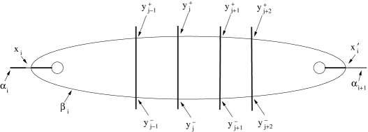
Figure 23. A $\beta$ handle in a Heegaard splitting of ${{K^{o}}}$.

Recall from section 3.2 that a knot complement admits a Heegaard splitting whose $\beta$ handles are the boundaries of regular neighborhoods of all but one of the overbridges. To label the $\alpha$ and $\beta$ handles of this splitting, we start at some underbridge, which we label $\alpha_{1}$, and travel along the knot, labeling the successive overbridges and underbridges $\beta_{1},\alpha_{2},\beta_{2}$, etc. We omit $\beta_{g}$, and twist up around $\alpha_{g}$. The resulting Heegaard diagram may be divided into three regions: the tubes, the interior regions bounded by the $\beta$’s in the plane of the diagram, and the exterior regions, which make up everything else in the plane of the diagram. We orient $m$ so that the basepoint $z_{s}$ lies in the exterior region.

As shown in Figure 23, most of the intersections of $\beta_{i}$ with the $\alpha$’s fall naturally into pairs $y_{j}^{\pm}$. The exceptions are the points at either end of the overbridge. We label these points $x_{i}$ (the intersection between $\beta_{i}$ and $\alpha_{i}$) and $x_{i}^{\prime}$ (the intersection between $\beta_{i}$ and $\alpha_{i+1}$).

Proposition 7.8.

The homological grading of the generator of ${{\widehat{HF}_{s}}}(K)$ is the same as the grading of ${\bf x}=\{x_{1},x_{2},\ldots,x_{g}\}$.

Before giving the proof, we pause to discuss the philosophy behind it. Like all Floer theories, the Ozsváth-Szabó  Floer homology is a Morse theory at heart. The Morse functional on ${{\widehat{CF}}}$ is the area function on $\Sigma$; i.e. if $\phi\in\pi_{2}({{{\bf y}}},{{{\bf z}}})$ with $n_{z}(\phi)=0$, ${{\mathcal{A}}}({{{\bf y}}})-{{\mathcal{A}}}({{{\bf z}}})$ is the signed area of ${{\mathcal{D}}}(\phi)$. Our ability to deform the metric on $\Sigma$ gives us great freedom to deform this Morse functional.

The set of generators for ${{\widehat{CF}_{s}}}({{\mathcal{H}}})$ may be complicated, but their homology is always very simple: ${{\widehat{HF}}}(S^{3})\cong{\bf{Z}}$. Now there is a well-known trick to turn a simple Morse function $f$ into a more complicated one. By making small perturbations, we can introduce cancelling pairs of critical points $v_{i}^{\pm}$, such that $f(v_{i}^{+})-f(v_{i}^{-})$ is very small and there is a unique differential from $v_{i}^{+}$ to $v_{i}^{-}$. For an appropriate choice of metric on $\Sigma$, ${{\widehat{CF}_{s}}}({{\mathcal{H}}})$ exhibits precisely this sort of behavior.

To be specific, the cancelling pairs will be of the form

$${{{\bf y}}}_{i}^{\pm}=\{y^{\pm}_{j},x_{1},x_{2},\ldots,x_{n},z_{1},\ldots,z_{g-n-1}\},$$

where $y^{\pm}_{j}$ is a pair of intersections like that of Figure 23 and the $z_{i}$’s are other points. The form of the domain of $\phi\in\pi_{2}({{{\bf y}}}_{i}^{+},{{{\bf y}}}_{i}^{-})$ is sketched in Figure 24. It is supported on the interior region and tubes of the Heegaard diagram. If we want ${{{\bf y}}}_{i}^{\pm}$ to behave like a pair of newly introduced critical points, the difference ${{\mathcal{A}}}({{{\bf y}}}_{i}^{+})-{{\mathcal{A}}}({{{\bf y}}}_{i}^{-})$ should be small. We can accomplish this for all of the pairs in question by taking the areas of the interior region and the tubes to be very small — much smaller than the area of any region in the exterior of the Heegaard splitting.

Next, we need to know that there is a differential from ${{{\bf y}}}_{i}^{+}$ to ${{{\bf y}}}_{i}^{-}$. For the moment, we simply state this as a fact, leaving the proof to the appendix.

Lemma 7.4.

There is a unique differential from ${{{\bf y}}}_{i}^{+}$ to ${{{\bf y}}}_{i}^{-}$ in ${{\widehat{CF}_{s}}}(E)$.

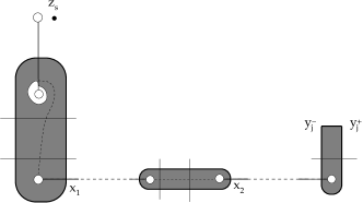
Figure 24. Domain of the differential from ${{{\bf y}}}_{i}^{+}$ to ${{{\bf y}}}_{i}^{-}$. The number of tubes in the domain can be anywhere from $0$ to $g-2$.

We refer to the differentials of this form as “short differentials.”

We now define an equivalence relation on the set of generators ${{{{\bf T}}_{\hat{\alpha}}\cap{{\bf T}}_{\hat{\beta}}}}$ by requiring that points connected by short differentials be equivalent. Every equivalence class contains $2^{m}$ elements of the form $\{y_{j_{1}}^{\pm},y_{j_{2}}^{\pm},\ldots,y_{j_{m}}^{\pm},z_{m+1},z_{m+2},\ldots,z_{g-1}\}$, where the $z_{i}$’s are “unpaired points” — either $x_{j}$ or $x_{j}^{\prime}$. For each equivalence class ${{\mathcal{Y}}}_{i}$, we let $I({{\mathcal{Y}}}_{i})$ be the smallest interval containing ${{\mathcal{A}}}({{{\bf y}}})$ for all ${{{\bf y}}}\in{{\mathcal{Y}}}_{i}$. We say that ${{\mathcal{Y}}}_{i}$ is isolated if $I({{\mathcal{Y}}}_{i})$ is disjoint from all of the other $I({{\mathcal{Y}}}_{j})$. Since the difference in ${{\mathcal{A}}}$ between two elements of the same equivalence class is much smaller than the difference between two elements in different classes, we expect that the ${{\mathcal{Y}}}_{i}$ should be isolated. This is indeed the case:

Lemma 7.5.

For a generic choice of large areas for the exterior regions of $\Sigma$, all equivalence classes are isolated.

Proof.

First, we observe that the length of $I({{\mathcal{Y}}})$ is bounded by $(g-1)$ times the area of the interior and tubular regions. Thus by choosing these areas to be sufficiently small, we can assume that all of the $I({{\mathcal{Y}}}_{i})$ have length less than $1$.

Suppose ${{{\bf y}}}_{1},{{{\bf y}}}_{2}\in{{{{\bf T}}_{\hat{\alpha}}\cap{{\bf T}}_{\hat{\beta}}}}$, and let $\phi\in\pi_{2}({{{\bf y}}}_{1},{{{\bf y}}}_{2})$. We claim that if ${{\mathcal{D}}}(\phi)$ is supported in the interior and tubular regions of $\Sigma$, then ${{{\bf y}}}_{1}$ and ${{{\bf y}}}_{2}$ are in the same equivalence class. Indeed, the components of the $\alpha$ curves in $\partial{{\mathcal{D}}}(\phi)$ must be supported in the interior regions. For homological reasons, they cannot go over the tubes. Thus they are either trivial or join some $y^{+}_{j}$ to the corresponding $y^{-}_{j}$. This implies the claim.

Next, we choose representative elements ${{{\bf y}}}_{i}\in{{\mathcal{Y}}}_{i}$ and topological disks $\phi_{ij}\in\pi_{2}({{{\bf y}}}_{i},{{{\bf y}}}_{j})$, and consider the differences ${{\mathcal{A}}}_{ij}={{\mathcal{A}}}({{{\bf y}}}_{i})-{{\mathcal{A}}}({{{\bf y}}}_{j})={{\mathcal{A}}}(\phi_{ij})$. The $\alpha$ and $\beta$ curves divide the exterior region into various components, each of whose areas we can vary separately. If $a_{k}$ is the area of the $k$th component, we have

$${{\mathcal{A}}}_{ij}=\sum_{k}n^{k}_{ij}a_{k}+C_{ij}$$

where $n^{k}_{ij}$ is the multiplicity of $\phi_{ij}$ over the $k$th component and $C_{ij}$ is the area of ${{\mathcal{D}}}(\phi_{ij})$ over the interior and tubular regions. If $i\neq j$, $y_{i}$ and $y_{j}$ are in different equivalence classes, so $n^{k}_{ij}\neq 0$ for some $k$.

To show that all of the ${{\mathcal{Y}}}_{j}$ are isolated, it suffices to show that $|A_{ij}|>2$ for all $i\neq j$. The set of $a_{k}$’s for which $|A_{ij}|<2$ is a width two neighborhood of some hyperplane in the space of all possible $a_{k}$’s. A finite union of such neighborhoods cannot fill up the entire positive quadrant, so the lemma is proved. ∎

Since differentials decrease ${{\mathcal{A}}}$, we have a filtration on ${{\widehat{CF}_{s}}}(E)$ whose filtered subquotients $C^{i}$ are generated by the elements of ${{\mathcal{Y}}}_{i}$.

Lemma 7.6.

If ${{\mathcal{Y}}}_{i}$ contains more than one element, the complex $C^{i}$ is acyclic.

Proof.

So far the only assumption we have made about the interior and tubular regions is that their total area is small. We now place some more specific requirements on the distribution of area within these regions. Without loss of generality, we assume that their total area should be bounded by 1.

First, we require that the total area of the interior regions should be very small — less than $4^{-g}$. Most of the area will be concentrated on the tubes. We assign the tube between $\beta_{g-1}$ and $\beta_{g-2}$ an area of $4^{1-g}$, the tube between $\beta_{g-1}$ and $\beta_{g-2}$ an area of $4^{2-g}$, and so on until we reach the tube between $\beta_{2}$ and $\beta_{1}$, which has an area of $4^{-2}$.

Fixing a particular equivalence class ${{\mathcal{Y}}}_{i}$, we say that the handle $\beta_{k}$ is active if the points in ${{\mathcal{Y}}}_{i}$ contain some $y_{j}^{\pm}$ on $\beta_{k}$, and inactive if they contain $x_{k}$ or $x_{k}^{\prime}$. If $\beta_{k_{1}},\beta_{k_{2}},\ldots,\beta_{k_{m}}$ is a list of the active $\beta$’s in order of increasing $k_{i}$, we can specify an element ${{{\bf y}}}\in{{\mathcal{Y}}}_{i}$ by a sequence of $m$ $+$’s and $-$’s, where the first $\pm$ determines whether $\beta_{k_{1}}$ contains $y^{+}$ or $y^{-}$, the second determines whether $\beta_{k_{2}}$ contains $y^{+}$ or $y^{-}$ on the next smallest, and so forth. With these conventions, it is easy to check that the ordering which ${{\mathcal{A}}}$ induces on the elements of ${{{\bf y}}}$ is the same as the lexicographic ordering on the sequence of $+$’s and $-$’s.

If ${{\mathcal{Y}}}_{i}$ has more than one element, we can use this area functional to filter $C^{i}$ so that each graded subquotient is generated by two elements of the form $w+$ and $w-$, where $w$ is some sequence of $+$’s and $-$’s. By Lemma 7.4, there is a unique differential from $w+$ to $w-$, so the filtered subquotients are all acyclic. Applying the reduction lemma, we see that $C^{i}$ is chain homotopy equivalent to a complex with no generators, so it is acyclic too. ∎

Proof.

(of Proposition 7.8) Together with the reduction lemma, the previous result shows that ${{\widehat{CF}_{s}}}(E)$ is chain homotopy equivalent to a complex generated by those ${{{\bf y}}}\in{{{{\bf T}}_{\hat{\alpha}}\cap{{\bf T}}_{\hat{\beta}}}}$ which are the unique elements in their equivalence classes. We claim that $\{x_{1},x_{2},\ldots x_{g}\}$ is the only such ${{{\bf y}}}$. Indeed, since we twisted up around $\alpha_{g}$, ${{{\bf y}}}$ cannot contain $x_{g}^{\prime}$. Thus it must contain $x_{g}$. But this implies it cannot contain $x_{g-1}^{\prime}$, so it must contain $x_{g-1}$, and so forth. ∎

7.7. A Model for Negative Surgeries

We conclude our discussion of the exact triangle by returning to the question raised at the end of section 7.4. As is often the case, it turns out to be more convenient to consider the exact triangle for negative $n$-surgery ($n\gg 0$):

$$\begin{CD}@>{}>{}>{{HF^{+}}}(N(0,1),{{\mathbf{s}}}_{k})@>{}>{}>{{HF^{+}}}({{\overline{N}}},{{\mathbf{s}}})@>{f}>{}>{{HF^{+}}}(N(-n,1),{{\mathbf{s}}}_{k})@>{}>{}>.\end{CD}$$

Figure 25. The short exact sequence $0\to C_{{{\mathbf{s}}}_{k}}\to{{CF_{r}^{+}}}(N,{{\mathbf{s}}})\to Q_{\psi_{k}}\to 0$.

The short exact sequence which models this triangle is shown in Figure 25. The dual of the quotient complex $Q_{{{\mathbf{s}}}_{k}}$ is the subcomplex of ${{CF_{r}^{\infty}}}(-N,{{\mathbf{s}}})$ which computes ${{HF^{-}}}(-N,{{\mathbf{s}}}_{k})$, so $H_{*}(Q_{{{\mathbf{s}}}_{k}})\cong{{HF^{+}}}(N(-n,1),{{\mathbf{s}}}_{k})$ for $n\gg 0$. Thus we have a long exact sequence

$$\begin{CD}@>{}>{}>H_{*}(C_{{{\mathbf{s}}}_{k}})@>{}>{}>{{HF^{+}}}({{\overline{N}}},{{\mathbf{s}}})@>{\pi_{s*}}>{}>{{HF^{+}}}(N(-n,1),{{\mathbf{s}}}_{k})@>{}>{}>.\end{CD}$$

We will prove

Theorem 7.1.

Suppose that ${{\mathbf{s}}}$ is a ${{\mathrm{Spin}^{c}}}$ structure on ${{\overline{N}}}$ which is fixed by the conjugation symmetry, and that this symmetry acts trivially on ${{\widehat{HF}}}({{\overline{N}}},{{\mathbf{s}}})$. Then for $k>0$, $\ker f\cong\ker\pi_{s*}$ and ${{\text{ \rm coker}\ }}f\cong{{\text{ \rm coker}\ }}\pi_{s*}$ as ${\bf{Q}}[u]$ modules.

In particular, the theorem applies to any knot in $\#^{n}(S^{1}\times S^{2})$.

The map $f$ is induced by the surgery cobordism $W$ from ${{\overline{N}}}$ to $N(-n,1)$. To be precise, let $x$ be the generator of $H^{2}(W)$ such that the pullback of $x$ to $N(-n,1)$ is ${{\mathbf{s}}}_{i+1}-{{\mathbf{s}}}_{i}$, and denote by ${{\mathfrak{t}}}_{i}$ the ${{\mathrm{Spin}^{c}}}$ structure on $W$ with $c_{1}({{\mathfrak{t}}}_{i})=ix$. (Note that ${{\mathfrak{t}}}_{i}$ is only defined for $i\equiv n\pod{2}$.) The restriction of ${{\mathfrak{t}}}_{i}$ to $N(n,1)$ is ${{\mathbf{s}}}_{(i-n)/2}$. (The easiest way to see this to take $n$ odd and consider ${{\mathfrak{t}}}_{\pm n}$, which induce the same ${{\mathrm{Spin}^{c}}}$ structure on $N(n,1)$. Since the ${{\mathfrak{t}}}_{\pm n}$ are conjugate symmetric, this ${{\mathrm{Spin}^{c}}}$ structure must be ${{\mathbf{s}}}_{0}$.) Then if $f_{i}{{\colon}}{{HF^{+}}}({{\overline{N}}})\to{{HF^{+}}}(N(-n,1),{{\mathbf{s}}}_{(i-n)/2})$ is the map defined by the pair $(W,{{\mathfrak{t}}}_{i})$,

$$f=\sum_{i\equiv n+2k\ (2n)}f_{i}.$$

It would be difficult to study all of the terms in this sum. When $n$ is large, however, we really only need to worry about $f_{\pm n+2k}$, which we call $f_{\pm}$ for short.

Lemma 7.7.

$\ker f=\ker{{\thinspace}}(f_{-}+f_{+})$ and ${{\text{ \rm coker}\ }}f\cong{{\text{ \rm coker}\ }}(f_{-}+f_{+})$.

Proof.

If $x\in{{HF^{+}}}({{\overline{N}}})$ is homogenous in grading, the grading formula tells us that

(4) $${{\mathrm{gr}}}{{\thinspace}}f_{-}(x)-{{\mathrm{gr}}}{{\thinspace}}f_{an+2k}(x)\geq\frac{-(-n+2k)^{2}+(an+2k)^{2}}{4n}=\frac{a^{2}-1}{4}n+(a+1)k\geq 0$$

since $n\gg k>0$. Thus $f_{-}$ has the smallest drop in absolute grading among all the $f_{i}$ appearing in the sum. Let us identify the relative gradings on ${{HF^{+}}}({{\overline{N}}},{{\mathbf{s}}})$ and ${{HF^{+}}}(N(-n,1),{{\mathbf{s}}}_{k})$ in such a way that $x$ and $f_{-}(x)$ have the same grading.

With this choice, we claim that there is some $m$ independent of $n$ such that $f$ is an isomorphism in degrees greater than $m$. Indeed, it suffices to choose $m$ so large that all elements in ${{HF^{+}}}(N(-n,1),{{\mathbf{s}}}_{k})$ and ${{HF^{+}}}({{\overline{N}}})$ with grading greater than $m$ are in the image of ${{HF^{\infty}}}$. Then the map

$$f_{\geq m}{{\colon}}{{HF^{+}}}({{\overline{N}}})_{\geq m}\to{{HF^{+}}}(N(-n,1),{{\mathbf{s}}}_{k})_{\geq m}$$

is the same as

$$f_{\geq m}^{\infty}{{\colon}}{{HF^{\infty}}}({{\overline{N}}})_{\geq m}\to{{HF^{\infty}}}(N(-n,1),{{\mathbf{s}}}_{k})_{\geq m}.$$

Since $f_{\geq m}^{\infty}=f_{-}^{\infty}+\epsilon$, where $f_{-}^{\infty}$ is an isomorphism and $\epsilon$ is strictly lower in degree, the claim holds.

We now observe that $\ker f=\ker f_{\leq m}$ and ${{\text{ \rm coker}\ }}f\cong{{\text{ \rm coker}\ }}f_{\leq m}$. The first equality is clear. To prove the second, we consider the composition

$${{\text{ \rm coker}\ }}f_{\leq m}=\frac{{{HF^{+}}}(N(-n,1),{{\mathbf{s}}}_{k})_{\leq m}}{{{\text{im}\ }}f_{\leq m}} {\hookrightarrow}\frac{{{HF^{+}}}(N(-n,1),{{\mathbf{s}}}_{k})}{{{\text{im}\ }}f_{\leq m}}$$

$$\to\frac{{{HF^{+}}}(N(-n,1),{{\mathbf{s}}}_{k})}{{{\text{im}\ }}f}={{\text{ \rm coker}\ }}f.$$

It is easy to check this map is an isomorphism.

On the other hand, when $n$ is very large, equation 4 implies that $f_{\leq m}=(f_{-}+f_{+})_{\leq m}$. Since $f_{-}+f_{+}$ is also an isomorphism on elements of degree $>m$, we have

$$\ker f=\ker f_{\leq m}=\ker(f_{+}+f_{-})_{\leq m}=\ker(f_{+}+f_{-})$$

$${{\text{ \rm coker}\ }}f\cong{{\text{ \rm coker}\ }}f_{\leq m}={{\text{ \rm coker}\ }}(f_{+}+f_{-})_{\leq m}\cong{{\text{ \rm coker}\ }}(f_{+}+f_{-}).$$

∎

Let $\pi_{s}{{\colon}}{{CF_{r}^{+}}}({{\overline{N}}})\to{{CF_{r}^{+}}}(N,{{\mathbf{s}}}_{k})$ be the projection.

Proposition 7.9.

Up to filtration preserving isomorphism of the target, $f_{-}=\pi_{s*}$.

To prove this, we study the map ${{f_{-}^{\infty}}}{{\colon}}{{CF^{\infty}}}({{\overline{N}}})\to{{CF^{\infty}}}(N(-n,1))$, which is defined by counting holomorphic triangles in the relevant Heegaard triple diagram. In Figure 26a, we show a portion of the spiral region for this diagram. (It lies on the cylinder obtained by identifying the top dotted line with the bottom one.) We position the attaching handle ${{\mathfrak{m}}}$ so that $w({{{\bf y}}})$ is on the stable side of ${{\mathfrak{m}}}$ for any generator ${{{\bf y}}}$ of ${{\widehat{CF}_{s}}}(N(-n,1))$. Then each such ${{{\bf y}}}$ has a unique small triangle $\Delta_{{{\bf y}}}$ connecting it to the corresponding generator ${{{\bf y}}}^{\prime}$ of ${{\widehat{CF}}}({{\overline{N}}})$. The part of the domain of this triangle which lies inside the spiral region is shown in the figure. It is easy to see that $\mu(\Delta_{{{\bf y}}})=0$ and $\#{\widehat{\mathcal{M}}}(\Delta_{{{\bf y}}})=\pm 1$.

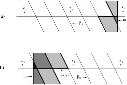
Figure 26. The Heegaard diagrams used to compute a) $f_{-}$ and b) $f_{+}$. In each figure, the domain of a typical triangles $\Delta_{{{\bf y}}}$ is shaded.

Lemma 7.8.

The ${{\mathrm{Spin}^{c}}}$ structure ${{\mathbf{s}}}_{z_{k}}(\Delta_{{{\bf y}}})$ determined by $\Delta_{{{{\bf y}}}}$ is ${{\mathfrak{t}}}_{-}$.

Proof.

Clearly ${{\mathbf{s}}}_{z_{k}}(\Delta_{{{\bf y}}})$ restricts to ${{\mathbf{s}}}_{k}$ on $N(-n,1)$. Let us take both $n$ and $k$ to be very large (but with $k<n$). Since $\#{\widehat{\mathcal{M}}}(\Delta_{{{\bf y}}})=\pm 1$ and $n_{z_{k}}(\Delta_{{{\bf y}}})=0$, ${{\mathbf{s}}}_{z_{k}}(\Delta_{{{\bf y}}})$ gives a nonzero map on ${{\widehat{CF}}}$. When $n$ is very large, the proof of Lemma 7.7 shows that this can happen only if ${{\mathbf{s}}}_{z_{k}}(\Delta_{{{\bf y}}})$ is equal to ${{\mathfrak{t}}}_{+}$ or ${{\mathfrak{t}}}_{-}$. Since $k$ is very large as well, the same argument shows that the degree of $f_{+}$ is much less than that of $f_{-}$, so it must be zero on ${{\widehat{CF}}}$ as well. Thus ${{\mathbf{s}}}_{z_{k}}(\Delta_{{{\bf y}}})={{\mathfrak{t}}}_{-}$ when $k$ is large. The result for arbitrary values of $k$ follows from the analogue of Lemma 2.12 of [19] for Whitney triangles. ∎

Lemma 7.9.

The map ${{f_{-}^{\infty}}}$ respects the bifiltration on ${{CF^{\infty}}}({{\overline{N}}})\cong{{CF^{\infty}}}(N(-n,1))$.

Proof.

For the stable filtration, this is just the fact that $n_{z_{k}}(\psi)\geq 0$ for any holomorphic triangle $\psi$. To prove it for the antistable filtration, suppose ${{{\bf y}}}$ is a generator of ${{\widehat{CF}}}(N(-n,1))$ and that ${{{\bf z}}}^{\prime}$ is a generator of ${{\widehat{CF}}}({{\overline{N}}})$ with the same ${\bf{Z}}/2$ grading as ${{{\bf y}}}$. (If the ${\bf{Z}}/2$ grading is different, ${{{\bf y}}}$ can never map to ${{{\bf z}}}^{\prime}$.) Let $\phi\in\pi_{2}({{{\bf y}}}^{\prime},{{{\bf z}}}^{\prime})$ be the unique disk with $\mu(\phi)=0$. Then $\psi=\Delta_{{{\bf y}}}\#\phi\in\pi_{2}({{{\bf y}}},\theta,{{{\bf z}}}^{\prime})$ has $\mu(\psi)=0$ and ${{\mathbf{s}}}_{z_{k}}(\psi)={{\mathfrak{t}}}_{-}$. Thus $\psi$ is the triangle which determines the ${{{\bf z}}}^{\prime}$ component of ${{f_{-}^{\infty}}}({{{\bf y}}})$. Since the $\beta_{g}$ component of $\psi$ is supported inside the spiral, the usual argument shows that ${{f_{-}^{\infty}}}$ preserves the Alexander grading. ∎

Proof.

(of Proposition 7.9) Since $f_{-}$ respects the bifiltration, we can reduce it to get a map ${{CF_{r}^{+}}}({{\overline{N}}})\to{{CF_{r}^{+}}}(N(-n,1),{{\mathbf{s}}}_{k})$, which we continue to denote by $f_{-}$. To prove the proposition, it suffices to show that ${{f_{-}^{\infty}}}$ induces an isomorphism on corresponding copies of ${{\mathcal{S}}}^{2}_{j}$. (The “dots” in the diagram.) This follows from a standard argument using the area filtration. We make the domains of the triangles $\Delta_{y}$ very small, so that their area is less than that of any other positive triangle. Then the map ${{\mathcal{S}}}^{1}_{j}({{\overline{N}}})\to{{\mathcal{S}}}^{1}_{j}(N(-n,1))$ has the form $1+\epsilon$, where $\epsilon$ decreases the area filtration. This proves the claim. ∎

Remark: This argument should be compared with the proof of Theorem 9.1 in [18]. In fact, the domains of the triangles used to define $f_{-}$ are closely related to the domains of the disks which define the differential $\delta_{1}$ described in that paper. We conjecture that $f_{-}$ and $\delta_{1}$ are actually the same map.

It seems difficult to compute the map $f_{+}$ from the Heegaard data of Figure 26a. The domains of the triangles defining this differential are related the domains of the disks which define the differential $\delta_{2}$ of [18]. In particular, they all have very large multiplicity.

Fortunately, there is another way to understand $f_{+}$. We use the slightly different Heegaard diagram of Figure 26b. The only thing that has changed in this figure is the position of the attaching handle ${{\mathfrak{m}}}$, which has been shifted so that all the $w({{{\bf y}}})$’s are on its antistable side. Thus the chain complex ${{CF^{+}}}(N(-n,1),{{\mathbf{s}}}_{k})$ remains the same. When we go to compute the Floer homology of ${{\overline{N}}}$, however, the basepoint $z_{k}$ is on the opposite side of ${{\mathfrak{m}}}$, so we get the complex ${{\widehat{CF}_{a}}}(N)$ rather than ${{\widehat{CF}_{s}}}(N)$. Let $\pi_{a}{{\colon}}CF^{+}_{ar}({{\overline{N}}})\to{{CF_{r}^{+}}}(N(-n,1),{{\mathbf{s}}}_{k})$ be the projection. Then the same arguments used to prove Proposition 7.9 imply

Proposition 7.10.

Up to filtered isomorphism of the target, $f_{+}=\pi_{a*}$.

Thus both $f_{-}$ and $f_{+}$ are induced by quotient maps at the chain level, but the maps are from a priori different complexes, both of which compute ${{HF^{+}}}({{\overline{N}}})$. By Proposition 4.3, however, there is an isomorphism $\iota{{\colon}}{{CF_{r}^{+}}}(N)\to{{CF_{a}^{+}}}(N)$, for which the induced map $\iota_{*}{{\colon}}{{HF^{+}}}({{\overline{N}}},{{\mathbf{s}}})\to{{HF^{+}}}({{\overline{N}}},{{\mathbf{s}}})$ is the conjugation symmetry. We will use this fact to prove the theorem.

Proof.

(Of Theorem 7.1) By hypothesis, $\iota_{*}$ acts trivially on ${{HF^{+}}}({{\overline{N}}},{{\mathbf{s}}})$, so

$$f_{-}+f_{+}=\pi_{s*}+(\pi_{a}\iota)_{*}.$$

If $A=\ker\pi_{s}$ and $B=\ker\pi_{a}\iota$, then the fact that $k>0$ implies that $A\subset B$.

We show that $\ker\pi_{s*}=\ker(\pi_{s*}+(\pi_{a}\iota)_{*})$. Indeed, if $\pi_{s*}(x)=0$, $x$ can be represented by a chain in $A$. Since $A\subset B$, $(\pi_{a}\iota)_{*}(x)=0$ as well. Conversely, suppose $\pi_{s*}(x)+(\pi_{a}\iota)_{*}(x)=0$. Write $x=x_{i}+x_{i-1}+\ldots$, where $x_{i}$ is homogenous of degree $i$. Since $k>0$, $(\pi_{a}\iota)_{*}(x_{j})$ has degree strictly lower than $\pi_{s*}(x_{j})$. Thus if we consider the equation $\pi_{s*}(x)+(\pi_{a}\iota)_{*}(x)=0$ one degree at a time, we obtain a series of equations

$$\pi_{s*}(x_{1}) =0 \pi_{s*}(x_{2}) =0 \ldots \pi_{s*}(x_{i-k}) =0$$

$$\pi_{s*}(x_{i-k-1}) =-(\pi_{a}\iota)_{*}(x_{1}) \pi_{s*}(x_{i-k-2}) =-(\pi_{a}\iota)_{*}(x_{2}) \ldots$$

Since $\pi_{s*}(x_{1})=0$, $x_{1}$ can be represented by a chain in $A$, so $(\pi_{a}\iota)_{*}(x_{1})=0$ as well. Thus $\pi_{s*}(x_{i-k-1})=0$. Repeating, we see that $\pi_{s*}(x_{j})=0$ for every $j$. This proves the claim.

To show that ${{\text{ \rm coker}\ }}\pi_{s*}\cong{{\text{ \rm coker}\ }}(\pi_{s*}+(\pi_{a}\iota)_{*})$, consider the map $g{{\colon}}{{CF_{r}^{+}}}(N,{{\mathbf{s}}}_{k})\to{{CF_{r}^{+}}}(N,{{\mathbf{s}}}_{k})$ given by $g=1+i\pi$, where $\pi$ is the projection which kills the remaining generators of $B$, and $i$ is the reflection isomorphism. Since $k>0$, $i$ strictly reduces the Alexander grading. This implies that $g$ is an isomorphism, so $g_{*}$ is an isomorphism on homology. Clearly $g(\pi_{s}(x))=\pi_{s}(x)+\pi_{a}\iota(x)$, so $g_{*}$ defines an isomorphism from ${{\text{ \rm coker}\ }}\pi_{s*}$ to ${{\text{ \rm coker}\ }}(\pi_{s*}+(\pi_{a}\iota)_{*})$.

∎

8. Alternating Knots

Among knots with small crossing number, perfect knots are very common. Our main result in this direction is Theorem 3, which states that alternating knots which satisfy a certain “smallness” condition are perfect. Small alternating knots are significantly more common than two-bridge knots; we have checked by computer that there is only one non-small alternating knot with fewer than 11 crossings ($10_{123}$ in Rolfsen’s tables) and only 6 non-small alternating knots with 11 crossings. In fact, the techincal condition of smallness is unnecessary: using a different Heegaard splitting from the one considered here, Ozsváth and Szabó have shown that all alternating knots are perfect.

Combining these facts with a few direct calculations, we have

Theorem 8.1.

All alternating knots with 10 or fewer crossings are perfect with $s(K)=\sigma(K)/2$. The same is true for nonalternating knots with 9 or fewer crossings, except for $8_{19}$ and $9_{42}$.

The proof of Theorem 3 is the main topic of this section. Afterwards, we briefly discuss computations for nonalternating knots and describe some interesting correspondences between ${{\widehat{CF}_{r}}}$ and Khovanov’s Jones polynomial homology.

8.1. Heegaard splittings and Generators

Let $K$ be an alternating knot. To compute ${{\widehat{CF}_{r}}}(K)$, we use a Heegaard splitting $(\Sigma,\alpha,\beta)$ of ${{K^{o}}}$ derived from a pair $({{\mathcal{D}}},c_{1})$, where ${{\mathcal{D}}}$ is an alternating diagram of $K$ and $c_{1}$ is a crossing of ${{\mathcal{D}}}$. The basic form of this splitting is shown in Figure 27. The genus of $\Sigma$ is the crossing number of $K$. Each edge of ${{\mathcal{D}}}$ corresponds to an $\alpha$ handle, and each crossing $c_{i}$ with $i>1$ corresponds to a $\beta$ handle $\beta_{i}$. Warning: such diagrams can be slightly misleading, since the “knot diagram” obtained by omitting the $\beta$’s is actually a diagram of $-K$! (Remember, the $\beta$’s are tubular neighborhoods of the overbridges.) Also, one must resist the temptation to attach the “tubes” to the two circles enclosed by a $\beta$ handle, rather than to the two ends of an edge.

Since the diagram is alternating, the $\alpha_{i}$’s and $\beta_{j}$’s all have the same local models. Each $\beta_{j}$ has two end intersections $x_{j}^{\pm}$ and two middle intersections $y_{j}^{\pm}$. The same is true for all of the $\alpha_{i}$’s, except that there is no $\beta_{1}$, so one $\alpha_{i}$ (call it $\alpha_{1}$) is missing its middle intersections, and two others are missing one of their end intersections.

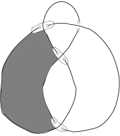
Figure 27. A Heegaard splitting of the complement of the figure 8 knot. The shaded region is the domain of a disk differential

We twist up around $\alpha_{1}$ and study the generators of the resulting complex ${{\widehat{CF}_{s}}}({{\mathcal{H}}})$. These generators are in one-to-one correspondence with the elements of ${{{{\bf T}}_{\hat{\alpha_{1}}}\cap{{\bf T}}_{\hat{\beta}}}}$. To describe them, we introduce the following

Definition 8.1.

A marked partial resolution (or MPR for short) of $K$ consists of the following data:

1. To each crossing $c_{i}$ with $i>1$, the assignment of either a resolution $\langle\smoothing\rangle$ or $\langle\hsmoothing\rangle$ or a sign $+$ or $-$.

2. A set of components of the resulting partially resolved diagram (the “marked components”) such that

   1. No marked component contains any unresolved crossings.

   2. Exactly one marked component passes through each resolved crossing.

Proposition 8.1.

The generators of ${{\widehat{CF}_{s}}}({{\mathcal{H}}})$ are in one-to-one correspondence with the set of marked partial resolutions of $K$.

Proof.

Suppose we are given a point ${{{\bf y}}}\in{{{{\bf T}}_{\hat{\alpha_{1}}}\cap{{\bf T}}_{\hat{\beta}}}}$. The corresponding marked resolution is constructed as follows. For each $i>1$, ${{{\bf y}}}$ contains a unique point on $\beta_{i}$, which is either a middle intersection or an end intersection. If it is a middle intersection, we label $c_{i}$ with a $\pm$, according to the sign of $y_{i}^{\pm}\in{{{\bf y}}}$. If it is an end intersection — call it $x$ —, we resolve $c_{i}$. Let $\alpha_{j}$ be the overbridge passing through $c_{i}$. Note that since $i\neq 1$, $j\neq 1$ as well. Thus ${{{\bf y}}}$ contains a point on $\alpha_{j}$. But $\alpha_{j}$’s middle intersections are not in ${{{\bf y}}}$, so exactly one if its end intersections must be. Call this end intersection $x^{\prime}$. We resolve $c_{i}$ so that the overbridge containing $x$ connects with the overbridge containing $x^{\prime}$, as illustrated in Figure 28. Finally, we mark the component containing $x$ and $x^{\prime}$.

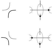
Figure 28. Resolving a crossing with an end intersection. The marked component is shown by the heavy line.

Let us check that the resulting diagram satisfies the definition of an MPR. The basic point is that we can “follow” a marked segment. If we start at a crossing $c_{i}$ containing an end intersection $x$, the marked segment takes us to a new end intersection $x^{\prime}$ in $c_{i^{\prime}}$. Thus $c_{i^{\prime}}$ must also be a resolved crossing. When we resolve it, the new marked segment continues the previous one. If we repeat this process, we must eventually return to our original end intersection $x$. It is clear from this description that a marked component does not contain any unresolved crossings. As for the second condition, a resolved crossing $c_{i}$ must contain one marked component by definition. It cannot contain more than one, since then both end intersections of $\beta_{i}$ would be in ${{{\bf y}}}$.

Now suppose we are given a marked partial resolution of $K$. The construction of the corresponding ${{{\bf y}}}\in{{{{\bf T}}_{\hat{\alpha}}\cap{{\bf T}}_{\hat{\beta}}}}$ is straightforward. Each $c_{i}$ with $i>1$ contributes an element of ${{{\bf y}}}$. If $c_{i}$ is marked $\pm$, ${{{\bf y}}}$ contains $y_{i}^{\pm}$. If $c_{i}$ is resolved, ${{{\bf y}}}$ contains whichever end intersection is on the marked component. We need to check that each $\alpha_{j}$ with $j>1$ contains a unique point in ${{{\bf y}}}$. If the crossing $c_{i}$ through which $\alpha_{j}$ passes is marked $\pm$, one of $\alpha_{j}$’s middle intersections is in ${{{\bf y}}}$, and neither end intersection is. (Such an end intersection would have to lie on a marked component passing through $c_{i}$.) On the other hand, if $c_{i}$ is resolved, exactly one end intersection of $\alpha_{j}$ is on a marked component. ∎

The generators corresponding to diagrams in which no crossing is resolved are of special interest to us:

Definition 8.2.

The base generators of ${{\widehat{CF}_{s}}}({{\mathcal{H}}})$ are the $2^{g-1}$ elements of ${{{{\bf T}}_{\hat{\alpha_{1}}}\cap{{\bf T}}_{\hat{\beta}}}}$ corresponding to MPRs in which every crossing (except $c_{1}$) is labeled with a $+$ or a $-$.

Recall that in section 4 we defined a grading $\tilde{\mu}={{\mathrm{gr}}}-A$ on ${{\widehat{CF}_{s}}}({{\mathcal{H}}})$.

Lemma 8.1.

All of the base generators have the same value of $\tilde{\mu}$.

Proof.

Let ${{{\bf y}}}^{+}=\{y_{1}^{\pm},y_{2}^{\pm},\ldots,y_{i}^{+},\ldots,y_{g}^{\pm}\}$ and ${{{\bf y}}}^{-}=\{y_{1}^{\pm},y_{2}^{\pm},\ldots,y_{i}^{-},\ldots,y_{g}^{\pm}\}$ be a pair of base generators whose signs differ at a single crossing. Then it is not difficult to see that ${{{\bf y}}}^{+}$ and ${{{\bf y}}}^{-}$ are connected by a punctured annular differential of the sort described in Lemma 7.4. Any two generators connected by such a differential have the same value of $\tilde{\mu}$. ∎

To prove Theorem 3, we will use the reduction lemma to compare ${{\widehat{CF}_{s}}}({{\mathcal{H}}})$ with a complex generated by a subset of the basepoint generators. The first step in this process is to divide the generators of ${{\widehat{CF}_{s}}}({{\mathcal{H}}})$ into groups. To every ${{{\bf y}}}\in{{{{\bf T}}_{\hat{\alpha_{1}}}\cap{{\bf T}}_{\hat{\beta}}}}$, we assign a base generator $b({{{\bf y}}})$ by leaving all the labeled crossings of the MPR of ${{{\bf y}}}$ unchanged and replacing each resolved crossing with a $+$ or a $-$, depending on whether the marked component contains $y_{i}^{+}$ or $y_{i}^{-}$. This assignment divides $E$ into $2^{g-1}$ equivalence classes, each containing a single base generator. We denote the class containing the base generator ${{{\bf y}}}$ by ${{\mathcal{Y}}}({{{\bf y}}})$.

8.2. Disk Differentials

We now describe a special class of differentials between elements in the same equivalence class. An example of such a differential for the figure-eight knot is shown in Figure 27. The following lemma guarantees that the shaded domain actually has $\#{\widehat{\mathcal{M}}}(\phi)=\pm 1$.

Lemma 8.2.

Suppose ${{\mathcal{D}}}(\phi)$ is a multiplicity one disk with all interior corners. Then $\mu(\phi)=1$ and $\#{\widehat{\mathcal{M}}}(\phi)=\pm 1$.

The proof is given in the appendix.

More generally, suppose $C$ is a marked component of the MPR for ${{{\bf y}}}\in E$. $C$ bounds two disks in the $S^{2}$ of the diagram. We say that $C$ is small if one of these disks does not have any crossings in its interior. In this case, $C$ bounds a disk ${{\mathcal{D}}}(\phi)$ in $\Sigma$. Near a crossing, ${{\mathcal{D}}}(\phi)$ looks like the local models shown in Figure 29. ${{\mathcal{D}}}(\phi)$ satisfies the conditions of Lemma 8.2, so we get a differential between ${{{\bf y}}}$ and another generator ${{{\bf y}}}^{\prime}$, whose MPR is obtained by “forgetting” $C$, i.e replacing each end intersection on $C$ by the adjacent middle intersection. Clearly ${{{\bf y}}}$ and ${{{\bf y}}}^{\prime}$ are in the same equivalence class.

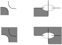
Figure 29. ${{\mathcal{D}}}(\phi)$ in the neighborhood of a crossing.

Motivated by this fact, we make the following

Definition 8.3.

An alternating knot $K$ is small if there is some diagram ${{\mathcal{D}}}$ of $K$ and choice of crossing $c_{1}$ such that every marked component of every MPR of $({{\mathcal{D}}},c_{1})$ is small.

From now one, we assume that $K$ is a small knot, and that $({{\mathcal{D}}},c_{1})$ is the corresponding small diagram. We call the differentials described above disk differentials. Since their domains are supported away from the spiral region, disk differentials preserve the Alexander grading. Thus all the elements of ${{{{\bf T}}_{\hat{\alpha_{1}}}\cap{{\bf T}}_{\hat{\beta}}}}$ in a given equivalence class have the same Alexander grading. Moreover, any element in an equivalence class can be connected to its base generator by a series of disk differentials, so it is easy to work out the homological grading on ${{\widehat{CF}_{s}}}({{\mathcal{H}}})$. (These statements still hold even if $K$ is not small.)

All the disk differentials in a given equivalence class are compatible with each other in the following sense:

Lemma 8.3.

Suppose ${{{\bf y}}}$ is a base generator, and let

$${{\mathcal{C}}}({{{\bf y}}})=\{C{{\thinspace}}|{{\thinspace}}C\ \text{is a marked component of an MPR}\ {{{\bf z}}}\ \text{with}\ b({{{\bf z}}})={{{\bf y}}}\}.$$

Then no two elements of ${{\mathcal{C}}}({{{\bf y}}})$ pass through the same crossing of $K$.

Proof.

Two elements of ${{\mathcal{C}}}({{{\bf y}}})$ which share an edge must be the same. Indeed, if we are given an edge of $C\in{{\mathcal{C}}}({{{\bf y}}})$, we can reconstruct $C$ by following it along from one crossing to the next. Each time we come to a new vertex, ${{{\bf y}}}$ tells us which way the resolution has to go. Suppose $C_{1},C_{2}\in{{\mathcal{C}}}({{{\bf y}}})$ are two different components coming into the same crossing. They must leave by the same edge, which contradicts the fact that they are different. ∎

Corollary 8.1.

The elements of ${{\mathcal{Y}}}({{{\bf y}}})$ are in bijective correspondence with subsets of ${{\mathcal{C}}}({{{\bf y}}})$.

Proof.

Given an MPR ${{{\bf y}}}^{\prime}\in{{\mathcal{Y}}}({{{\bf y}}})$, we map it to its set of marked components. In the other direction, given $\{C_{1},C_{2},\ldots,C_{m}\}\subset{{\mathcal{C}}}({{{\bf y}}})$, we start with the MPR for ${{{\bf y}}}$ and resolve all the crossings contained in the $C_{i}$. By Lemma 8.3, no crossing is contained in more than one of the $C_{i}$. Thus we can resolve each crossing to get the $C_{i}$’s, and then mark them to get a valid MPR. It is easy to check that these two procedures define inverse maps. ∎

8.3. Cancellation

The remainder of the proof is similar to the proof of Proposition 7.8. We use the area functional to filter ${{\widehat{CF}_{s}}}({{\mathcal{H}}})$ so that all the generators in an equivalence class are in the same filtered subquotient. Next, we use a cancellation argument to show that any equivalence class with more than one element is acyclic. Finally, we apply the reduction lemma to prove the theorem.

Lemma 8.4.

For an appropriate choice of metric on $\Sigma$, the ${{\mathcal{Y}}}({{{\bf y}}})$ are all isolated in the sense of Lemma 7.5.

Proof.

We choose a metric on $\Sigma$ in which the area of all the exterior regions put together is much less than the area of any one of the tubes. Any ${{{\bf y}}}\in E$ is connected to $b({{{\bf y}}})$ by a sequence of disk differentials whose domains contain only exterior regions. Thus it suffices to show that there is a choice of areas on the tubes for which the base generators are widely separated. Since the base generators are connected by annular differentials, this can be accomplished by an argument like that of Lemma 7.6. ∎

We take such a metric and use the resulting area functional to filter ${{\widehat{CF}_{s}}}({{\mathcal{H}}})$ so that each filtered subquotient is generated by the elements of some ${{\mathcal{Y}}}({{{\bf y}}})$.

Lemma 8.5.

If ${{\mathcal{Y}}}({{{\bf y}}})$ contains more than one element, the complex it generates is acyclic.

Proof.

By Corollary 8.1, the elements of ${{\mathcal{Y}}}({{{\bf y}}})$ correspond to subsets of ${{\mathcal{C}}}({{{\bf y}}})$. If ${{\mathcal{C}}}({{{\bf y}}})$ has $n$ elements, we can represent each ${{{\bf y}}}^{\prime}\in{{\mathcal{Y}}}({{{\bf y}}})$ by a sequence ${s_{i}}$ of $n$ $1$’s and $0$’s, where $s_{i}$ is $1$ if $C_{i}\in{{\mathcal{C}}}({{{\bf y}}})$ is marked, and $0$ if it is not. With this convention, it is easy to see that

$$A(\{s_{i}\})=\sum_{i=1}^{n}s_{i}a_{i}$$

where $a_{i}$ is the signed area of of the disk domain bounded by $C_{i}$. (The sign of $a_{i}$ is determined by whether the differential goes to or from the MPR with the marked component.)

We now argue as in Lemma 7.6. We are free to vary the $a_{i}$’s, so long as we keep them small, so we take e.g. $a_{i}=4^{1-i}a_{1}$. With this choice, the area filtration splits the complex generated by ${{\mathcal{Y}}}({{{\bf y}}})$ into $2^{n-1}$ subquotients, each containing two generators connected by the disk differential corresponding to $C_{n}$. By the reduction lemma, $C({{{\bf y}}})$ is acyclic. ∎

Proof.

(Of Theorem 3.) The area filtration restricts to a filtration on the complex ${{\mathcal{S}}}_{1}^{j}({{\mathcal{H}}})$. Since disk differentials preserve the Alexander grading, all of the elements of a given ${{\mathcal{Y}}}({{{\bf y}}})$ belong to the same ${{\mathcal{S}}}_{1}^{j}$. Then Lemma 8.4 shows that we can filter ${{\mathcal{S}}}_{1}^{j}({{\mathcal{H}}})$ so that each filtered subquotient is generated by some ${{\mathcal{Y}}}({{{\bf y}}})$. By Lemma 8.5 and the reduction lemma, ${{\mathcal{S}}}_{1}^{j}({{\mathcal{H}}})$ is chain homotopy equivalent to a complex generated by those base generators ${{{\bf y}}}$ such that $A({{{\bf y}}})=j$ and ${{\mathcal{Y}}}({{{\bf y}}})$ contains no elements other than ${{{\bf y}}}$. But by Lemma 8.1, all base generators have the same value of $\tilde{\mu}$. Thus ${{\widehat{CF}_{r}}}(K)$ is perfect. ∎

8.4. Small knots

Although the condition of smallness is seems quite restrictive, there are some infinite families of small knots.

Lemma 8.6.

Any two bridge knot is small. Any alternating three-strand pretzel knot is small.

Proof.

Any two bridge knot has an alternating diagram like that shown in Figure 30a. If we choose $c_{1}$ as shown, any marked component of an MPR of $D$ must be supported in the columns labeled 1 and 2, so it cannot have any crossings in its interior. A very similar argument applies to the three-strand pretzel knot shown in part b of the figure. ∎

Figure 30. A two-bridge knot and an alternating three-bridge pretzel knot. The special crossings $c_{1}$ are circled.

Thus we recover the result that two-bridge knots are perfect.

Unsurprisingly, alternating knots with small crossing number tend to be small. Using a computer, we have checked that the only nonsmall alternating knots with fewer than 12 crossings are $10_{123}$, $11^{a}_{236}$, $11^{a}_{327}$,$11^{a}_{335}$,$11^{a}_{356}$,$11^{a}_{357}$, and $11^{a}_{366}$ . (Knots with 10 or fewer crossings are labeled according to Rolfsen’s tables in [26]; knots with more crossings are identified by their Knotscape number.) As the crossing number increases, however, it seems clear that the fraction of alternating knots which are small will tend to zero.

9. Appendix on Differentials

In this appendix, we collect some explicit results about the differentials in the Ozsváth-Szabó  complex. The fundamental question in this area is “which domains correspond to differentials?” In other words, given the domain ${{\mathcal{D}}}(\phi)$ of a topological disk $\phi$, we would like to be able to determine $\mu(\phi)$ and, if $\mu(\phi)=1$, $\#{\widehat{\mathcal{M}}}(\phi)$ from the combinatorial information contained in the Heegaard diagram. Below, we give a formula for $\mu(\phi)$. This formula has a purely combinatorial interpretation for a wide class of domains, and it should be possible to extend this interpretation to all domains. In contrast, $\#{\widehat{\mathcal{M}}}(\phi)$ may not be determined by the combinatorics of the diagram. (See Lemma 5.7 of [19] for an example.) Still, there are many useful cases in which it is. We describe two such cases — disky differentials and punctured annular differentials — which were used in sections 7 and 8.

9.1. Domains

We begin by reviewing the definition of ${{\mathcal{D}}}(\phi)$ (Lemma 3.6 of [19].) Given $\phi\in\pi_{2}({{{\bf y}}},{{{\bf z}}})$, we choose some map $u{{\colon}}{D}^{2}\to s^{g}{\Sigma}$ representing $\phi$ and consider the incidence correspondence

$$S=\{(x,y)\in{D}^{2}\times\Sigma{{\thinspace}}|{{\thinspace}}y\in u(x)\}.$$

Without loss of generality, we can choose $u$ transverse to the diagonal in $s^{g}{\Sigma}$, so that the projection $\pi_{1}{{\colon}}S\to{D}^{2}$ is a $g$-fold branched covering map.

The projection $\pi_{2}{{\colon}}S\to{\Sigma}_{g}$ defines a singular $2$–chain in $\Sigma_{g}$, and thus (since $\partial S$ maps to $\alpha\cup\beta$), a cellular $2$–chain ${{\mathcal{D}}}(\phi)$ in the cellulation of $\Sigma_{g}$ defined by $\alpha$ and $\beta$. ${{\mathcal{D}}}(\phi)$ depends only on $\phi$. Indeed, its multiplicity on a given cell is the intersection number $n_{w}(\phi)$ between $\phi$ and ${w}\times s^{g-1}{\Sigma}_{g}$, where $w$ is a point in the interior of the cell.

We mark the two points on $\partial D^{2}$ which map to ${{{\bf y}}}$ and ${{{\bf z}}}$. Their inverse images under $\pi_{1}$ give rise to $2g$ marked points on $\partial S$. Since $\pi_{1}{{\colon}}\partial S\to\partial D^{2}$ is a covering map, $\pi_{2}$ sends these marked points alternately to the $y_{i}$’s and and the $z_{j}$’s. The segments between them map alternately to $\alpha$ and $\beta$. As a result, the cellular chain $\partial{{\mathcal{D}}}(\phi)$ is composed of $2g$ arcs, one on each of the $\alpha$ and $\beta$–circles. Each $y_{i}$ and $z_{j}$ is the endpoint of one such arc and the starting point of another. Conversely, it is not difficult to see that any null-homologous 1-chain satisfying these conditions bounds ${{\mathcal{D}}}(\phi)$ for some $\phi\in\pi_{2}({{{\bf y}}},{{{\bf z}}})$.

Figure 31. A typical example in which $\partial{{\mathcal{D}}}(\phi)$ and $\pi_{2}(\partial S)$ differ. Varying the length of the “tail” in $\pi_{2}(\partial S)$, changes the modulus of $S$.

We refer to the $y_{i}$’s and $z_{j}$’s collectively as the corner points of ${{\mathcal{D}}}(\phi)$. If $y_{i}=z_{j}$ for some $i$ and $j$, the corresponding corner point is degenerate. An arc joining a degenerate corner to itself may be degenerate as well. If both arcs are degenerate, we say that the corner point is isolated. For example, the corner points of the trivial disk $\theta\in\pi_{2}({{{\bf y}}},{{{\bf y}}})$ are all isolated.

It is worth pointing out that even when $u$ is holomorphic, the singular chain $\partial S$ need not be equal to the cellular chain $\partial{{\mathcal{D}}}(\phi)$, but only homologous to it. This fact will be relevant when we study the Maslov index, since varying the singular chain will change the complex structure on $S$. A typical example of this phenomenon is shown in Figure 31.

9.2. The Maslov index

In this section, we describe how to compute $\mu(\phi)$ from the domain of $\phi$. We state the basic formula here, but postpone its proof to the next section.

Figure 32. The local multiplicities for the various possible corner points. The two intersecting lines are $\alpha_{i}$ and $\beta_{j}$; $\partial{{\mathcal{D}}}(\phi)$ is shown in bold. Types c), d), and e) are degenerate; d) is isolated.

Theorem 9.1.

(5) $$\mu(\phi)=2\chi({{\mathcal{D}}}(\phi))+\phi\cdot\Delta+\sum_{i=1}^{2g}n(c_{i}).$$

The terms in this formula are to be interpreted as follows. $\chi({{\mathcal{D}}}(\phi))$ is the Euler characteristic of ${{\mathcal{D}}}(\phi)$ as a cellular chain. In other words, it is $\chi(T)$, where $T$ is a surface with boundary $\partial{{\mathcal{D}}}(\phi)$ which maps to $\Sigma$ as an unbranched cover with multiplicities given by ${{\mathcal{D}}}(\phi)$. (This definition extends to domains with negative multiplicities, via the relation $\chi({{\mathcal{D}}}(\phi)+\Sigma)=\chi({{\mathcal{D}}}(\phi))+2-2g$.) Note that $\partial T$ need not map to isolated corner points of $\phi$. For example, if $\theta\in\pi_{2}({{{\bf y}}},{{{\bf y}}})$ is the trivial disk, $T$ is the empty set. The second term is the intersection number of $\phi$ with the diagonal $\Delta$ in $s^{g}{\Sigma}_{g}$. Since ${{\bf T}}_{\alpha}$ and ${{\bf T}}_{\beta}$ are disjoint from $\Delta$, this number is well defined. Finally, the numbers $n(c_{i})$ are certain local multiplicities of the $2g$ corner points of ${{\mathcal{D}}}(\phi)$. These numbers depend only on the geometry of $\partial{{\mathcal{D}}}(\phi)$ in a neighborhood of the corner point. The local multiplicities of the different possible corners are shown in Figure 32. Note that the local multiplicity of any degenerate corner point is $0$.

The first and last terms in Equation 5 are easily computed from ${{\mathcal{D}}}(\phi)$, but the middle term is not as obvious. We explain how to evaluate it in the special case when $\partial{{\mathcal{D}}}(\phi)$ is planar, that is, when we can surger ${\Sigma}_{g}$ along $g$ circles disjoint from $\partial{{\mathcal{D}}}(\phi)$ to get a sphere. This procedure associates to each domain ${{\mathcal{D}}}(\phi)$ in $\Sigma$ a new domain ${{\mathcal{D}}}(\phi^{\prime})$ in $S^{2}$, together with $2g$ marked points $p_{1}^{\pm},p_{2}^{\pm},\ldots,p_{g}^{\pm}$ (the centers of the surgery disks.) It is not difficult to see that ${{\mathcal{D}}}(\phi^{\prime})$ determines a homotopy class of disks $\phi^{\prime}$ in $s^{g}S^{2}\cong{\bf CP}^{g}$.

Let us consider the simpler problem of finding the intersection number of $\phi^{\prime}$ with the diagonal $\Delta_{S^{2}}$ in $s^{g}S^{2}$. Suppose there is a point $w\in S^{2}$ with $n_{w}(\phi^{\prime})=0$. We put $w$ at infinity, so that $\phi$ can be represented by a disk in $s^{g}{\bf{C}}={\bf{C}}^{g}$. In this case, we can use the well-known identification of $\pi_{1}({\bf{C}}^{g}-\Delta_{{\bf{C}}})$ with the braid group $B_{g}$. We briefly recall this correspondance here. Suppose we are given a loop in ${\bf{C}}^{n}-\Delta_{{\bf{C}}}$. By the usual incidence construction, we get maps $\pi_{1}\colon C\to S^{1}$ and $\pi_{2}\colon C\to{\bf{C}}$, where $\pi_{1}$ is a $g$-fold covering map. Let $\pi_{1}^{-1}(1)=\{a_{1},\ldots,a_{g}\}$. If $g\colon[0,1]\to S^{1}$ is the standard generator of $\pi_{1}(S^{1})$ and $\tilde{g}_{i}\colon[0,1]\to C$ is the lift of $g$ which starts at $a_{i}$, we set $\gamma_{i}=\pi_{2}\circ g_{i}$. Then the curves $\Gamma_{i}(t)=(\gamma_{i}(t),t))$ define the associated braid in ${\bf{C}}\times{\bf{R}}\cong{\bf{R}}^{3}$.

To apply this construction to $\partial{{\mathcal{D}}}(\phi^{\prime})$, we take $\gamma_{i}$ to be the curve which starts at $y_{i}$, travels along an $\alpha$-segment of $\partial{{\mathcal{D}}}(\phi^{\prime})$ until it reaches some $z_{j}$, and then continues along a $\beta$-curve to $y_{k}$. We denote the resulting braid by $\beta(\phi^{\prime})$.

It is easy to see that the abelianization of $B_{g}$ is ${\bf{Z}}$ and that the quotient homomorphism $t\colon B_{g}\to{\bf{Z}}$ is the map which sends a braid to its writhe. On the other hand, the map $\pi_{1}({\bf{C}}^{g}-\Delta_{\bf{C}})\to{\bf{Z}}$ which sends a loop to its linking number with $\Delta$ factors through the abelianization and has $1$ in its image. (Just take a small loop around a smooth point of $\Delta_{\bf{C}}$.) Thus it agrees with $t$ up to a factor of $\pm 1$. Checking the sign, we see that $\phi^{\prime}\cdot\Delta_{\bf{C}}=t(\beta(\phi^{\prime}))$. Example: Suppose ${{\mathcal{D}}}(\phi^{\prime})$ has the form shown in Figure 33a. The corresponding braid has writhe two, so $S$ is a double branched cover of $D^{2}$ branched at two points; i.e. an annulus. The map $\pi_{2}$ pinches one component of $\partial S$ down to a T–shaped loop supported on $\alpha$ and $\beta$.

Figure 33. ${{\mathcal{D}}}(\phi)$ and $\beta(\phi)$.

We now drop the hypothesis that $n_{w}(\phi^{\prime})=0$ and put an arbitrary point of $S^{2}-\alpha-\beta$ at infinity. Let $L\in\pi_{2}({\bf CP}^{g})$ be the class of a line. Then $n_{w}(L)=1$ for any $w$ and $L\cdot\Delta_{S^{2}}=2g-2$ (since ${{\mathcal{D}}}(L)=S^{2}$ is a branched $g$-fold cover of $S^{2}$). The connected sum $\phi_{1}^{\prime}=\phi^{\prime}\#(-n_{\infty}(\phi^{\prime})L)$ has $n_{\infty}(\phi_{1}^{\prime})=0$, so

$$\phi_{1}^{\prime}\cdot\Delta_{S^{2}} =t(\beta(\phi_{1}^{\prime}))=t(\beta(\phi^{\prime}))\quad\text{and}$$

$$\phi^{\prime}\cdot\Delta_{S^{2}} =(2g-2)n_{\infty}(\phi^{\prime})+t(\beta(\phi^{\prime})).$$

Finally, we return to the problem of determining $\phi\cdot\Delta$. Let $S\subset({\Sigma})^{g}$ and $S^{\prime}\subset(S^{2})^{g}$ be the surfaces determined by $\phi$ and $\phi^{\prime}$. We would like to understand the relationship between them. If

$$D_{i}^{\pm}=\{(x_{1},\ldots x_{g})\subset(S^{2})^{g}{{\thinspace}}|{{\thinspace}}x_{j}=p_{i}^{\pm}\text{ for some }j\},$$

a generic $S^{\prime}$ will intersect $D_{i}^{\pm}$ transversely at smooth points of $D_{i}^{\pm}$. The surface $S$ is by obtained by embedding $(S^{2})^{g}-\cup D_{i}^{\pm}$ in $(\Sigma_{g})^{g}$ in the obvious way. The image of $S^{\prime}$ under this embedding will be a punctured surface. Each puncture created by $D_{i}^{+}$ will have a corresponding puncture created by $D_{i}^{-}$, and $S$ is obtained by filling in each pair of punctures with a copy of the appropriate annulus in ${\Sigma}_{g}$. To compute the effect of this procedure on $\phi\cdot\Delta$, note that each added annulus results in two more branch points of $\pi_{1}$, and thus in an additional two intersections with the diagonal. To determine the sign of these intersections, we use the following lemma, whose proof is a straightforward calculation in local coordinates.

Lemma 9.1.

If $\pi_{1}{{\colon}}S\to D^{2}$ is an orientation preserving branched cover and $x\in S$ is a branch point of $\pi_{1}$, the sign of the corresponding intersection with $\Delta$ is the local degree of $\pi_{2}$ at $x$.

It follows that the total contribution to the intersection number coming from $V_{i}$ is twice the multiplicity of ${{\mathcal{D}}}(\phi)$ over $V_{i}$, which is in turn equal $n_{p_{i}^{+}}({{\mathcal{D}}}(\phi^{\prime}))+n_{p_{i}^{-}}({{\mathcal{D}}}(\phi^{\prime}))$.

To summarize, we see that we have proved the following

Proposition 9.1.

If $\partial{{\mathcal{D}}}(\phi)$ is a planar curve in ${\Sigma}_{g}$ and ${{\mathcal{D}}}(\phi^{\prime})$ is its associated domain in $S^{2}$, then

$$\phi\cdot\Delta=(2g-2)n_{\infty}({{\mathcal{D}}}(\phi^{\prime}))+t(\beta(\phi^{\prime}))+\sum_{i=1}^{g}[n_{p_{i}}^{+}(\phi^{\prime})+n_{p_{i}}^{-}(\phi^{\prime})].$$

Remark: When $\partial{{\mathcal{D}}}(\phi)$ is not a planar curve, it should be possible to evaluate $\phi\cdot\Delta$ by thinking about the braid defined by $\phi$ in the braid group of the punctured surface ${\Sigma}_{g}-pt$. The abelianization of this group is ${\bf{Z}}\oplus{\bf{Z}}^{2g}$, with the first summand corresponding to the linking number of $\partial\phi$ with $\Delta$ and the second summand corresponding to the class of $\partial\phi$ in $H_{1}(s^{g}{\Sigma}_{g})\cong H_{1}({\Sigma}_{g})$. Thus the problem is to find an approriate generalization of the writhe for the braid group of a punctured surface.

9.3. Proof of Theorem 9.1

Before starting the proof, we give an alternate formulation of equation 5 together with a heuristic argument explaining why this formula should be true.

Suppose for the moment that $\phi$ is actually represented by a holomorphic map $u$, so that the maps $\pi_{1}{{\colon}}S\to D^{2}$ and $\pi_{2}{{\colon}}S\to\Sigma_{g}$ are branched covers with $b_{1}=g-\chi(S)$ and $b_{2}$ branch points. The surface $S$ is equipped with two pieces of data: a complex structure and a system of $2g$ marked points on its boundary. We can reconstruct this data either from the branched cover over the disk or from the branched cover over $\Sigma_{g}$: in order for there to be a holomorphic disk, the two reconstructions must agree. Over the disk, $S$ is determined by the location of the $b_{1}$ branch points. Over $\Sigma_{g}$, we can vary the location of $b_{2}$ branch points, but we may also be able to vary the complex structure on $S$ by “cutting” the boundary of ${{\mathcal{D}}}(\phi)$ near the corner points, as illustrated in Figure 31. Each direction we can cut in gives us an additional real parameter. We denote the number of parameters we get at the corner $c_{i}$ by $\nu(c_{i})$. The possible values of $\nu$ are shown in Figure 34. Thus we have a total of $2b_{1}+2b_{2}+\sum\nu(c_{i})$ free parameters. (Each degenerate corner contributes only once to the sum, not twice.) On the other hand, the space of complex structures on $S$ has dimension $-3\chi(S)$, and the marked points are determined by another $2g$ real parameters. Subtracting, we get

$$\mu(\phi) =2(g-\chi(S))+2b_{2}+\sum\nu(c_{i})-(2g-3\chi(S))$$

$$=\chi(S)+2b_{2}+\sum\nu(c_{i}).$$

Figure 34. Possible values of $\nu$. Darker shading indicates regions of greater multiplicity.

To see that this is equivalent to equation 5, we would like to write $\chi(S)=b_{2}+\chi({{\mathcal{D}}}(\phi))$. This is not quite correct, however, since boundary components of $S$ will collapse to isolated corner points. We can account for this fact by adding a correction term $\sum m(c_{i})$ to the right-hand side, where $m$ is $+1$ for a corner point of type e) (which results in an extra disk, and $-1$ for a point of type f) (which results in an extra puncture.) Then we have

$$\chi(S)+2b_{2}+\sum\nu(c_{i}) =2\chi(D)-\chi(S)+\sum[\nu(c_{i})+2m(c_{i})]$$

$$=2\chi(D)+\phi\cdot\Delta-g+\sum[\nu(c_{i})+2m(c_{i})]$$

$$=2\chi(D)+\phi\cdot\Delta+\sum n(c_{i})$$

where in the last step we have distributed the factor of $-g$ over the sum, adding a $-1/2$ to each ordinary corner and a $-1$ to each degenerate corner. We leave it to the reader to check that the resulting contributions agree with the values of $n(c_{i})$ given in section 9.2.

To actually prove the theorem, we attempt to represent $\phi$ by a map $u$ which is similar to a holomorphic map, in the sense that $\pi_{1}$ and $\pi_{2}$ are orientation preserving branched covers. We will not always achieve this goal, but we can control the situations in which it fails to hold.

Lemma 9.2.

If equation 5 holds for those $\phi$ with ${{\mathcal{D}}}(\phi)\geq 0$, it holds for all $\phi$.

Proof.

Let $E\in\pi_{2}(s^{g}{\Sigma})$ be the positive generator. Then ${{\mathcal{D}}}(E)={\Sigma}$ is a $g$–fold cover of $S^{2}$ branched at $E\cdot\Delta$ points, so $E\cdot\Delta=4g-2$. Given $\phi\in\pi_{2}({{{\bf y}}},{{{\bf z}}})$, consider $\phi^{\prime}=\phi\#nE$. Then ${{\mathcal{D}}}(\phi^{\prime})={{\mathcal{D}}}(\phi)+n{\Sigma}\geq 0$ for $n\gg 0$, so

$$\mu(\phi^{\prime}) =2\chi({{\mathcal{D}}}(\phi^{\prime}))+\phi^{\prime}\cdot\Delta+\sum n(c_{i})$$

$$\mu(\phi)+2n =2\chi({{\mathcal{D}}}(\phi)+n(2-2g))+\phi\cdot\Delta+n(4g-2)+\sum n(c_{i})$$

$$\mu(\phi) =2\chi({{\mathcal{D}}}(\phi))+\phi\cdot\Delta+\sum n(c_{i}).$$

∎

Definition 9.1.

Suppose we are given $\pi_{2}\colon S\to{\Sigma}_{g}$. A collapsed tube of $\pi_{2}$ is an annulus $A\cong S^{1}\times[-1,1]\subset S$ such that $\pi_{2}|_{A}$ factors through the projection to $[-1,1]$.

Lemma 9.3.

If ${{\mathcal{D}}}(\phi)\geq 0$, then there is a representative $u$ of $\phi$ for which $S$ is a nodal surface, $\pi_{1}\colon S\to D^{2}$ is an orientation preserving branched cover, and $\pi_{2}\colon S\to{\Sigma}_{g}$ is an orientation preserving branched cover away from a finite union of collapsed tubes.

Proof.

Our first step is to construct a branched covering map $p_{2}\colon T\to{{\mathcal{D}}}(\phi)$ such that $\partial T$ maps to the path $\partial{{\mathcal{D}}}(\phi)$. To do so, we start with $n_{z_{i}}(\phi)$ copies of the cell $\mathcal{C}_{i}$, where $z_{i}\in\mathcal{C}_{i}$. We glue these cells together along their edges in a maximal fashion, so that when we are done, there are no unglued edges which project to the same edge in ${\Sigma}$ with opposite orientation. (Of course, there are many such gluings; we just choose one.). Thus we obtain a surface $T_{0}$ with a projection $p_{0}{{\colon}}T_{0}\to{\Sigma}$. The map $p_{0}$ is a covering map except at the vertices of the cellulation, where it may be branched. Since the gluing was maximal, $p_{0}(\partial T_{0})$ is equal to $\partial{{\mathcal{D}}}(\phi)$ as a chain. The two may not be equal as paths, however, since $p_{0}(\partial T_{0})$ may “turn a corner” at a vertex where $\partial{{\mathcal{D}}}(\phi)$ goes straight. To solve this problem, we slit the two components of $T_{0}$ near the vertex in question and glue them back in the opposite way. This introduces another branch point in the projection. After making these modifications, we obtain the desired surface $T$ and map $p_{2}{{\colon}}T\to{\Sigma}$.

Next, we let $T^{\prime}$ be a connected surface obtained by taking the connected sum of all components of $T$. Then we can find a map $p_{2}^{\prime}{{\colon}}T^{\prime}\to{\Sigma}_{g}$ which agrees with $p_{2}$ away from the connected sum regions, and for which each connected sum region is a collapsed tube. Since $T^{\prime}$ is connected, there is a $g$-fold covering map $p_{1}^{\prime}{{\colon}}T^{\prime}\to D^{2}$ which has precisely two branch points in each collapsed tube. We immerse $T^{\prime}$ in $D^{2}\times{\Sigma}_{g}$ via the map $p_{1}^{\prime}\times p_{2}^{\prime}$. When $p_{1}^{\prime}$ and $p_{2}^{\prime}$ are generic, the image will have isolated double points, none of which are contained in the collapsed tubes. We define $S$ to be this image and $\pi_{1}$ and $\pi_{2}$ to be the projections onto the two factors. With these maps, the hypotheses of the lemma are clearly satisfied. ∎

Proof.

(of Theorem 9.1) The Maslov index of $\phi$ is defined as follows [29]. Choose a complex structure $J$ on $s^{g}{\Sigma}$. Let $p{{\colon}}I^{2}\to D^{2}$ be the map from unit square to the disk which collapses the two vertical sides, and choose any map $u{{\colon}}D^{2}\to s^{g}{\Sigma}$ which represents $\phi$. Then $E=(up)^{*}Ts^{g}{\Sigma}$ is a (necessarily trivial) bundle of complex vector spaces over the square. We define a family $L$ of Lagrangian subspaces on $E|_{\partial I^{2}}$ by pulling back the tangent spaces of ${{\bf T}}_{\alpha}$ and ${{\bf T}}_{\beta}$. To be precise, we identify the tangent spaces at ${{{\bf y}}}$ and ${{{\bf z}}}$ with ${\bf{C}}^{g}$ in such a way that $T{{\bf T}}_{\alpha}={\bf{R}}^{n}$ and $T{{\bf T}}_{\beta}=i{\bf{R}}^{n}$, and set

$$L_{(s,0)} =(up)^{*}T{{\bf T}}_{\alpha}$$

$$L_{(s,1)} =(up)^{*}T{{\bf T}}_{\beta}$$

$$L_{(*,t)} =e^{i\pi t/2}{\bf{R}}^{n}\quad(*=0,1).$$

If we choose a trivialization $E\cong I^{2}\times{\bf{C}}^{g}$, $L$ defines a loop in the space $\Lambda_{g}$ of totally real subspaces of ${\bf{C}}^{g}$, and $\mu(\phi)$ is the class of this loop in $\pi_{1}(\Lambda_{g})\cong{\bf{Z}}$. Equivalently, it is the obstruction to extending $L$ to a family of totally real subspaces on all of $I^{2}$. (Note that this definition differs from the usual one in that we use totally real spaces rather than Lagrangians. The reason is that the symplectic form on $s^{g}{\Sigma}_{g}$ does not extend across the diagonal. Since the space of totally real subspaces deformation retracts to the space of Lagrangians, this has no effect on the definition.)

Without loss of generality, we may assume ${{\mathcal{D}}}(\phi)\geq 0$ and that the map $u$ is of the form described in Lemma 9.3. To compute $\mu(\phi)$, we consider a slightly different family of Lagrangians on the square. To define this family, we round off the corners of $S$ to get a smooth manifold $S^{\prime}$. Then $T(\partial S^{\prime})$ is a natural family of Lagrangian subspaces of $TS^{\prime}|_{\partial S^{\prime}}$. $L^{\prime}$ is defined to be the push-forward of this family. More precisely, we choose $\pi_{1}^{\prime}{{\colon}}S^{\prime}\to I^{2}$ and $\pi_{2}^{\prime}{{\colon}}S^{\prime}\to{\Sigma}_{g}$ which agree with $\pi_{1}$ and $\pi_{2}$ except near the corners. Then if $x_{1},\ldots,x_{g}$ are the preimages of $(s,t)\in\partial I^{2}$ under $\pi_{1}^{\prime}$, we can identify $E_{(s,t)}$ with $(T({\Sigma})^{g})_{(x_{1},x_{2},\ldots,x_{g})}$. Under this identification, $L^{\prime}_{(s,t)}$ is the space spanned by the vectors $(0,\ldots,d\pi_{2}(T(\partial S^{\prime})_{x_{i}}),\ldots,0)$, where the nonzero entry is in the $i$th position.

By construction, $L^{\prime}$ and $L$ agree on the horizontal sides of the square, but they may differ on the vertical sides. To compute $\mu(L)-\mu(L^{\prime})$, we note that on the vertical sides, $L$ and $L^{\prime}$ decompose into a direct sum in the sum of the tangent spaces near each corner: $L=\oplus_{c_{i}}L(c_{i})$ and $L^{\prime}=\oplus_{c_{i}}L^{\prime}(c_{i})$, where $L_{c_{i}}$ is one dimensional if $c_{i}$ is an ordinary corner and two-dimensional if $c_{i}$ is degenerate. Thus we can write

$$\mu(L)-\mu(L^{\prime})=\sum_{c_{i}}\mu(L(c_{i}))-\mu(L^{\prime}(c_{i}))=\sum_{c_{i}}n(c_{i})$$

where the numbers $n(c_{i})$ depend only on the local geometry of the corner $c_{i}$.

We now concentrate on finding $\mu(L^{\prime})$. To do so, we try to write down an extension of $L^{\prime}$ to the entire square, and then study the places where this extension fails to exist. The induced orientation on $\partial S^{\prime}$ determines a nonvanishing vector field ${\bf v}$ on $\partial S^{\prime}$. We pick an extension of ${\bf v}$ to $S^{\prime}$ satisfying the following conditions. Near each collapsed tube, ${\bf v}$ should be chosen so that it can be extended to a nonzero vector field on the surface obtained by surgering the tube. (Thus ${\bf v}$ defines a vector field on the surface $T$ of Lemma 9.3.) Elsewhere, ${\bf v}$ should vanish at isolated points, none of which are nodes of $S$. There will be $\chi(T)$ such points, counted with sign. Away from these points, ${\bf v}$ determines a family of Lagrangians on $S^{\prime}$. We try to extend $L^{\prime}$ to the entire square by pushing this family of Lagrangians forward in the same way we defined $L^{\prime}$. There are four sorts of places where this extension might fail to exist:

1. Branch points of $\pi_{1}$ not on the nodes or collapsed tubes.

2. Branch points of $\pi_{2}$ not on the nodes or collapsed tubes.

3. Nodal points of $S$.

4. The collapsed tubes.

5. Points where v vanishes.

Without loss of generality, we can assume that all branch points of type 1) and 2) are simple and that the images of each collapsed tube is supported in a small neighborhood of some point in the square. Moreover, we can assume that all these points have disjoint images under $\pi_{1}$. Let $\{x_{i}\}\subset I^{2}$ be the set of these images, and let $\gamma_{i}$ be a small circle centered at $x_{i}$. Then

$$\mu(L^{\prime}|_{\partial I^{2}})=\sum\mu(L^{\prime}|_{\gamma_{i}}).$$

Computing $\mu(L^{\prime}|_{\gamma_{i}})$ is a local problem, which we can study individually for each of the types listed above.

Lemma 9.4.

Suppose that $x_{i}$ is a point of type 1). Then $\mu(L^{\prime}|_{\gamma_{i}})=1$.

Proof.

Let $U_{i}$ be a small disk centered at $x_{i}$ and containing $\gamma_{i}$. Without loss of generality, we can choose ${\bf v}$ to be a constant vector field on each component of $\pi_{1}^{-1}(U_{i})$. Then $L^{\prime}|_{\gamma_{i}}=L_{1}\oplus L_{2}$, where $L_{1}$ is a $2$–dimensional Lagrangian coming from the component with the branch point, and $L_{2}$ is a constant Lagrangian coming from the other $g-2$ components. Thus $\mu(L^{\prime}|_{\gamma_{i}})=\mu(L_{1})$.

To evaluate $\mu(L_{1})$, we use the following local model: $\gamma_{i}$ is the unit circle in ${\bf{C}}$, $\pi_{1}{{\colon}}D^{2}\to D^{2}$ is the map $z\to z^{2}$, and $\pi_{2}{{\colon}}D^{2}\to{\bf{C}}$ is the identity map. The corresponding $u{{\colon}}D^{2}\to s^{2}{\bf{C}}$ sends $z\to\{\sqrt{z},-\sqrt{z}\}$. Identifying $s^{2}{\bf{C}}$ with ${\bf{C}}^{2}$ by the map which sends $\{u,v\}\to(u+v,uv)$, we see that $u{{\colon}}D^{2}\to{\bf{C}}^{2}$ is given by $u(z)=(0,-z)$. Then a tangent vector $\alpha$ at the point $\sqrt{z}\in S$ pushes forward to the tangent vector $(\alpha,-\sqrt{z}\alpha)\in T{\bf{C}}^{2}|_{(0,-z)}$. Since ${\bf v}$ is a constant vector field, it pushes forward to define

$$L_{1}=\{((\alpha+\beta){\bf v},(\beta-\alpha)\sqrt{z}{\bf v})\subset u^{*}(T{\bf{C}}^{2})|_{z}\ |{{\thinspace}}\alpha,\beta\in{\bf{R}}\}.$$

Thus $L_{1}$ is the direct sum of a trivial family of Lagrangians in the first factor with a family with Maslov index 1 in the second factor, so $\mu(L_{1})=1$. ∎

Lemma 9.5.

Suppose that $x_{i}$ is a point of type 2). Then $\mu(L^{\prime}|_{\gamma_{i}})=2$.

Proof.

As in the previous lemma, we choose ${\bf v}$ to be constant on each component of $\pi_{1}^{-1}(U_{i})$. Then $L^{\prime}|_{\gamma_{i}}$ splits as a direct sum, and the only contribution to the Maslov index will come from the summand containing the branch point. In this case, there is a local model in which $\pi_{1}{{\colon}}D^{2}\to D^{2}$ is the identity map and $\pi_{2}{{\colon}}D^{2}\to D^{2}$ is the map $z\to z^{2}$. Then $u{{\colon}}D^{2}\to D^{2}$ is also given by $z\to z^{2}$, and the constant vector field ${\bf v}$ pushes forward to the vector field $z{\bf v}$. It is easy to see that the Maslov index of the associated family of Lagrangians is 2. ∎

Lemma 9.6.

If $x_{i}$ is a point of type 3), then $\mu(L^{\prime}|_{\gamma_{i}})=2{{\thinspace}}\text{sign}{{\thinspace}}x_{i}$, where $\text{sign}{{\thinspace}}x_{i}$ is the sign of the intersection in $D^{2}\times{\Sigma}_{g}$.

Proof.

As before, we see that $\mu(L^{\prime}|_{\gamma_{i}})=\mu(L_{1})$, where $L_{1}$ is a two-dimensional family of Lagrangians pushed forward from the two components of $S$. Near $x_{i}$, a local model for the two sheets of $S$ is given by

$$S=\{({{{\bf x}}},A{{{\bf x}}}){{\thinspace}}|{{\thinspace}}{{{\bf x}}}\in{\bf{R}}^{2}\}\cup\{({{{\bf x}}},B{{{\bf x}}}){{\thinspace}}|{{\thinspace}}{{{\bf x}}}\in{\bf{R}}^{2}\}$$

where $A$ and $B$ are invertible $2\times 2$ matrices. The maps $\pi_{1}$ and $\pi_{2}$ are the projections onto the first and second coordinates, and the map $u{{\colon}}D^{2}\to{\bf{C}}^{2}$ is given by $u({{{\bf x}}})=(A{{{\bf x}}}+B{{{\bf x}}},(A{{{\bf x}}})(B{{{\bf x}}}))$, where the parentheses indicate complex multiplication under the identification ${\bf{R}}^{2}={\bf{C}}$. If we choose ${\bf v}$ to be given by constant vectors ${\bf v}_{1}$ and ${\bf v}_{2}$ on the two components of $S$, we see that

$$L_{1}=\{(\alpha A{\bf v}_{1}+\beta B{\bf v}_{2},\alpha(A{\bf v}_{1})(B{{{\bf x}}})+\beta(B{\bf v}_{2})(A{{{\bf x}}})){{\thinspace}}|{{\thinspace}}\alpha,\beta\in{\bf{R}}\}.$$

To evaluate $\mu(L_{1})$, we choose ${\bf v}_{1}$ and ${\bf v}_{2}$ so that $A{\bf v}_{1}=B{\bf v}_{2}={\bf w}$. Then $L_{1}$ becomes

$$\{((\alpha+\beta){\bf w},(\alpha A{{{\bf x}}}+\beta B{{{\bf x}}}){\bf w})\}.$$

This family is totally real at all points on $\gamma_{i}$ whenever $A-B$ is nonsingular, so we can homotope $L_{1}$ to a similar family $L_{1}^{\prime}$ for which $A^{\prime}=A-B$ and $B^{\prime}=0$. It follows that $\mu(L_{1})=\mu(L_{1}^{\prime})=2\det(A-B)$.

On the other hand, the sign of $x_{i}$ as an intersection point is the sign of

$$\det\left(\begin{array}[]{cc}I&A\\ I&B\end{array}\right)=\det(A-B).$$

This proves the claim. ∎

Lemma 9.7.

If $x_{i}$ is a point of type 4), then $\mu(L^{\prime}|_{\gamma_{i}})=0$.

Proof.

If $u$ is a representative for $\phi$, we can always make another representative $u^{\prime}$ of $\phi$ by adding a collapsed tube to $S$. $u^{\prime}$ and $u$ have the same points of types 1)–3), and they obviously have the same Maslov index, so adding a collapsed tube must have no effect on $\mu$. ∎

Lemma 9.8.

If $x_{i}$ is a point of type 5), then $\mu(L^{\prime}|_{\gamma_{i}})=2{{\thinspace}}\text{ind}_{x_{i}}{\bf v}$.

Proof.

As in Lemmas 9.4 and 9.6, we can decompose $L^{\prime}|_{\gamma_{i}}=L_{1}\oplus L_{2}$, where $L_{1}$ is a constant Lagrangian and $L_{2}$ is the one-dimensional family of Lagrangians determined by ${\bf v}$ near the point at which it vanishes. It is then easy to check that $\mu(L_{2})=2{{\thinspace}}\text{ind}_{x_{i}}{\bf v}$. ∎

Since the sum of $\text{ind}_{x_{i}}{\bf v}$ over all points of type 5) is $\chi(T)$, we have

$$\mu(L^{\prime}_{\partial_{I^{2}}}) =b_{1}+2b_{2}+2n+2\chi(T).$$

where $b_{1}$ and $b_{2}$ are the number of points of types 1) and 2) and $n$ is the signed number of nodes of $S$. We claim that $b_{1}+2n=\phi\cdot\Delta.$ To see this, recall that intersections of ${{\text{im}\ }}u$ with $\Delta$ correspond to branch points of $\pi_{1}$, and the sign of the intersection is the sign of the map $\pi_{2}$. By construction, branch points of type 1) have multiplicity one and positive sign. Next a local calculation like that of Lemma 9.6 shows that each node of $S$ corresponds to a point of tangency with $\Delta$, and the sign of the intersection corresponds to the sign of the intersection at the node. Thus the nodes contribute a total of $2n$ to the intersection number. Finally, the two branch points on each collapsed tube contribute with opposite signs. To see this, we perturb the map $\pi_{2}$ a bit, so the collapsed tube becomes a flattened tube, with the two branch points on opposite sides. This proves the claim.

Next, we observe (as in the heuristic argument) that $b_{2}+\chi(T)=\chi({{\mathcal{D}}}(\phi))$ up to correction factors of $\pm 1$ introduced by isolated corners. We lump these factors in with the $n(c_{i})$ to obtain a formula like that of equation 5.

Finally, we must determine the numbers $n(c_{i})$. For nondegenerate corners, this is a direct computation with one dimensional Lagrangians. For corners of type a), $n(c)=-1$ if $c$ is one of the $y_{i}$ and $0$ if $c$ is one of the $z_{i}$. Similarly, $n(c)$ is either $0$ or $1$ for corners of type b). Since the total number of $y_{i}$’s and $z_{i}$’s is equal, we can symmetrize these figures to arrive at the values shown in Figure 32. Corners of type c) are direct sums of a corner of type a) and a corner of type b), so they have $n=0$. Finally, we evaluate $n$ for corners of type d) and e) by applying the formula to domains for which $\mu$ is known. ∎

9.4. The Localization Principle

We now turn our attention to the problem of determining whether a given domain admits a differential. There are two basic principles to keep in mind here. First, ${{\mathcal{D}}}(\phi)$ must be positive whenever $\#{\widehat{\mathcal{M}}}(\phi)\neq 0$. Second, $\#{\widehat{\mathcal{M}}}(\phi)$ is a local quantity: it depends only on the geometry in a small neighborhood of the domain. More precisely, suppose ${{\mathcal{D}}}(\phi)$ is a positive domain. Define the support of $\phi$ (written $\overline{{{\mathcal{D}}}}(\phi)$) to be the union of all cells with nonzero multiplicities in ${{\mathcal{D}}}(\phi)$ and all corner points of ${{\mathcal{D}}}(\phi)$. Then we have

Lemma 9.9.

If $U$ is any open neighborhood of $\overline{{{\mathcal{D}}}}(\phi)$, and we choose a generic path of almost complex structures $J_{s}$ which is sufficiently close to a complex structure $J$ induced by a complex structure on ${\Sigma}$, then the image of any $J_{s}$-holomorphic representative of $\phi$ is contained in $s^{g}U$.

Proof.

Suppose that the statement is false. Then we can choose a sequence $J^{i}_{s}$ of generic $J_{s}$’s converging to $J$, for which there are $J_{s}$–holomorphic representatives $u^{i}$ of $\phi$ whose image is not contained in $s^{g}U$. By passing to a subsequence, we can assume there is a sequence of points $x^{i}\not\in s^{g}U$ with $x_{i}\in{{\text{im}\ }}u^{i}$ and $x^{i}\to x$ for some $x\not\in s^{g}U$. Then by Gromov compactness, we obtain a (possibly degenerate) $J$-holomorphic representative $u$ of $\phi$ with $x\in{{\text{im}\ }}u$. In this case, the corresponding map $\pi_{2}{{\colon}}S\to{\Sigma}$ is holomorphic, so it is either open and orientation-preserving or constant on each irreducible component of $S$. The image of each connected component of $S$ must contain a corner point, so $\pi_{2}(S)=\overline{{{\mathcal{D}}}}(\phi)\subset U$. But this contradicts the fact that $x\not\in s^{g}U$. ∎

As a first application of this localization principle (Ozsváth and Szabó’s phrase), we show that to study differentials, it suffices to consider connected domains. More precisely, suppose that $\overline{{{\mathcal{D}}}}(\phi)$ can be divided into two disjoint domains $\overline{{{\mathcal{D}}}}(\phi_{1})$ and $\overline{{{\mathcal{D}}}}(\phi_{2})$ containing $g_{1}$ and $g_{2}$ corner points. We let ${{\bf T}}_{\alpha_{1}}\subset s^{g_{1}}{\Sigma}_{g}$ be the product of those $\alpha_{i}$’s containing corner points of ${{\mathcal{D}}}(\phi_{1})$, ${{{\bf y}}}_{1}\in s^{g_{1}}{\Sigma}_{g}$ be the set of those $y_{i}$’s in ${{\mathcal{D}}}(\phi_{1})$, etc. Then ${{\mathcal{D}}}(\phi_{i})$ defines a homotopy class $\phi_{i}\in\pi_{2}({{{\bf y}}}_{i},{{{\bf z}}}_{i})$ of disks in $s^{g_{i}}{\Sigma}_{g}$, and we have

Proposition 9.2.

$\mu(\phi)\cong\mu(\phi_{1})+\mu(\phi_{2})$ and ${\widehat{\mathcal{M}}}(\phi)\cong{\widehat{\mathcal{M}}}(\phi_{1})\times{\widehat{\mathcal{M}}}(\phi_{2})$.

Proof.

If $U_{1}$ and $U_{2}$ are disjoint open sets containing $\overline{{{\mathcal{D}}}}(\phi_{1})$ and $\overline{{{\mathcal{D}}}}(\phi_{1})$, the localization principle tells us that the image of any holomorphic representative $u$ of $\phi$ is contained in $s^{g}(U_{1}\cup U_{2})$. In fact, it must be in the connected component of this set containing ${{{\bf y}}}$ and ${{{\bf z}}}$, which is $s^{g_{1}}U_{1}\times s^{g_{2}}U_{2}$. Similarly, it is not difficult to see that $\partial u$ must actually lie on ${{\bf T}}_{\alpha_{1}}\times{{\bf T}}_{\alpha_{2}}\cup{{\bf T}}_{\beta_{1}}\times{{\bf T}}_{\beta_{2}}$. Thus we are really studying maps of a holomorphic disk into a product. In this case, it is well-known that the Maslov index and moduli spaces of $J$-holomorphic representatives behave as stated.

∎

Corollary 9.1.

If $\mu(\phi)=1$ and $\overline{{{\mathcal{D}}}}(\phi)=\overline{{{\mathcal{D}}}}(\phi_{1})\coprod\overline{{{\mathcal{D}}}}(\phi_{2})$, then ${\widehat{\mathcal{M}}}(\phi)$ is empty unless one component (say $\overline{{{\mathcal{D}}}}(\phi_{2})$) is a union of isolated points, in which case ${\widehat{\mathcal{M}}}(\phi)\cong{\widehat{\mathcal{M}}}(\phi_{1})$.

Proof.

This is the standard connected sum argument from gauge theory. Since $\mu(\phi)=1$, we can assume without loss of generality that $\mu(\phi_{2})\leq 0$. If it is negative, ${\widehat{\mathcal{M}}}(\phi_{2})$ is generically empty. If it is $0$ and ${\widehat{\mathcal{M}}}(\phi_{2})$ is nonempty, the ${\bf{R}}$ action on it is not free, so the corresponding map is constant. In this case ${{\mathcal{D}}}(\phi_{2})$ is a union of isolated points and $\#{\widehat{\mathcal{M}}}(\phi_{2})=1$. ∎

9.5. Examples of Differentials

We conclude by proving the existance of the differentials used in sections 7 and 8. The basic idea is to use the localization principle and the invariance of ${{\widehat{CF}_{r}}}$ to show that the domain in question must give a differential. We start with the “punctured annular differential” $\phi$ whose domain is shown in Figure 24, i.e. $\phi\in\pi_{2}({{{\bf y}}}_{+},{{{\bf y}}}_{-})$, where ${{{\bf y}}}_{\pm}=\{x_{1},\ldots,x_{n},y_{\pm}\}$.

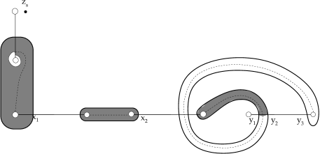
Figure 35. A Heegaard splitting of the trefoil ($n=2$).

Lemma 9.10.

The disk $\phi$ described above has $\mu(\phi)=1$ and $\#{\widehat{\mathcal{M}}}(\phi)=\pm 1$ for any $J_{s}$ sufficiently close to a complex structure $J$.

Proof.

Consider the Heegaard splitting of the trefoil shown in Figure 35. It is easy to see that ${{\widehat{CF}_{s}}}$ for this diagram is generated by ${{{\bf y}}}_{i}=\{x_{1},x_{2},\ldots,x_{n},y_{i}\}$, and that $A(y_{i})=i$. The domain of the unique $\psi\in\pi_{2}({{{\bf y}}}_{1},{{{\bf y}}}_{2})$ with $n_{z_{s}}(\psi)=0$ is shaded. We claim that $\mu(\psi)=1$ and $\#{\widehat{\mathcal{M}}}(\psi)=\pm 1$. When $n=1$, this is Lemma 8.4 of [19]. The result for general $n$ then follows from the fact that ${{\widehat{CF}_{r}}}$ is an invariant. The domain of $\psi$ is combinatorially identical to the domain of $\phi$, except that the latter domain may be cut by other $\beta$–curves, as shown in Figure 24. These segments are inaccessible — they cannot be connected to the corner points through a region of positive multiplicity. By the localization principle, they cannot be in the image of $\partial S$, and are thus irrelevant to the problem of determining $\#{\widehat{\mathcal{M}}}(\phi)$. By varying the conformal structure of the surface in Figure 35, we can make ${{\mathcal{D}}}(\psi)$ conformally equivalent to ${{\mathcal{D}}}(\phi)$, so $\#{\widehat{\mathcal{M}}}(\phi)=\#{\widehat{\mathcal{M}}}(\psi)=\pm 1$.

∎

Next, we consider “disky differentials.”

Lemma 9.11.

If the domain of $\phi\in\pi_{2}({{{\bf y}}},{{{\bf z}}})$ is an embedded disk with all interior corners, then $\mu(\phi)=1$ and $\#{\widehat{\mathcal{M}}}(\phi)=\pm 1$.

Proof.

Consider the diagram of the unknot shown in Figure 36. The stable complex of this knot has three generators: ${{{\bf x}}}_{1}=\{x_{1},z_{1},z_{2},\ldots,z_{n-1}\}$, ${{{\bf x}}}_{2}=\{x_{2},z_{1},z_{2},\ldots,z_{n-1}\}$, and ${{{\bf y}}}=\{y_{1},y_{2},\ldots,y_{n}\}$. It’s easy to see that $A({{{\bf x}}}_{2})=A({{{\bf z}}})\neq A({{{\bf x}}}_{1})$, so by the invariance of ${{\widehat{CF}_{r}}}$, there must be a cancelling differential between ${{{\bf x}}}_{2}$ and ${{{\bf z}}}$. The unique $\psi\in\pi_{2}({{{\bf z}}},{{{\bf x}}}_{2})$ with $n_{z_{s}}(\psi)=0$ has the shaded disk in the figure as its domain. Since the domain of the corresponding $\psi^{\prime}\in\pi_{2}({{{\bf x}}}_{2},{{{\bf z}}})$ is negative (in fact, ${{\mathcal{D}}}(\psi^{\prime})=-{{\mathcal{D}}}(\psi)$), we must have $\mu(\psi)=1$ and $\#{\widehat{\mathcal{M}}}(\psi)=\pm 1$. By varying the metric on $\Sigma$, we can make ${{\mathcal{D}}}(\psi)$ conformally equivalent to ${{\mathcal{D}}}(\phi)$, which proves the lemma. ∎

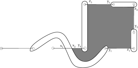
Figure 36. A disky differential in a diagram for the unknot ($n=4$).

References

- [1] P. Braam and S. Donaldson. Floer’s work on instanton homology, knots, and surgery. In The Floer Memorial Volume, pages 195–256. Birkhauser, 1995.
- [2] R.H. Crowell and R.H. Fox. Introduction to Knot Theory. Ginn and Co., 1963.
- [3] R. Fintushel and R. Stern. Instanton homology of Seifert-fibred homology spheres. Proc. London Math. Soc., 61:109–137, 1990.
- [4] A. Floer. Witten’s complex and infinite dimensional Morse theory. J. Differential Geom., 30:207–21, 1989.
- [5] K.A. Frøyshov. Equivariant aspects of Yang-Mills Floer theory. Topology, 41:525–552, 2002.
- [6] K.A. Frøyshov. Lectures at Harvard University. Spring 2001.
- [7] L. Kauffman. On Knots. Annals of Mathematics Studies, 115. Princeton University Press, 1987.
- [8] M. Khovanov. A categorification of the Jones polynomial. Duke Math. J., 101:359–426, 2000.
- [9] M. Khovanov. Patterns in knot cohomology i. math.QA/0201306, 2002.
- [10] P. Kirk, E. Klassen, and D. Ruberman. Splitting the spectral flow and the Alexander matrix. Comment. Math. Helv., 69:375–416, 1994.
- [11] P. B. Kronheimer. Embedded surfaces and gauge theory in three and four dimensions. In Surveys in Differential Geometry, Vol. III, pages 243–298. Int. Press, 1998.
- [12] P. B. Kronheimer and T. S. Mrowka. 1996 I.P. lecture.
- [13] E. S. Lee. Khovanov’s invariants for alternating links. math.GT/0210213, 2002.
-
[14]
C. Manolescu.
Seiberg-Witten-Floer stable homotopy type of three-manifolds with
.
math.DG/0104024, 2001. - [15] J. McCleary. User’s Guide to Spectral Sequences. Mathematics Lecture Series, 12. Publish or Perish Inc, 1985.
- [16] C. McMullen. The Alexander polynomial of a 3-manifold and the Thurston norm on cohomology. Ann. Sci. École Norm. Sup. (4), 35:153–171, 2002.
- [17] T. Mrowka, P. Ozsváth, and B. Yu. Seiberg-Witten monopoles on Seifert-fibred spaces. Comm. Anal. Geom., 4:685–791, 1997.
- [18] P. Ozsváth and Z. Szabó. Holomorphic disks and three-manifold invariants: properties and applications. To appear in Annals of Mathematics. math.SG/0105202.
- [19] P. Ozsváth and Z. Szabó. Holomorphic disks and topological invariants for rational homology three-spheres. To appear in Annals of Mathematics. math.SG/0101206.
- [20] P. Ozsváth and Z. Szabó. Absolutely graded Floer homologies and intersection forms for four-manifolds with boundary. math.SG/0110170, 2001.
-
[21]
P. Ozsváth and Z. Szabó.
Holomorphic triangles and invariants for smooth four-manifolds.
math.SG/0110169, 2001. - [22] P. Ozsváth and Z. Szabó. Heegaard Floer homology and alternating knots. math.GT/0209149, 2002.
- [23] P. Ozsváth and Z. Szabó. Holomorphic disks and knot invariants. math.GT/0209056, 2002.
- [24] P. Ozsváth and Z. Szabó. Knot Floer homology and the four-ball genus. math.GT/0301026, 2003.
- [25] J. Rasmussen. Floer homology of surgeries on two-bridge knots. Algebraic and Geometric Topology, 2:757–89, 2002. math.GT/020405.
- [26] D. Rolfsen. Knots and Links. Mathematics Lecture Series, 7. Publish or Perish Inc., 1976.
- [27] H. Schubert. Knoten mit zwei Brücken. Math. Z., 65:133–70, 1956.
- [28] V. Turaev. Torsion invariants of structures on 3-manifolds. Math. Res. Lett., 4:679–695, 1997.
- [29] C. Viterbo. Intersection de sous-variétés lagrangiennes, fonctionelles d’action, et indice des systèmes hamiltoniens. Bull. Soc. Math. France, 115:361–390, 1987.