First Steps in Tropical Geometry

Abstract.

Tropical algebraic geometry is the geometry of the tropical semiring $(\mathbb{R},{\rm min},+)$. Its objects are polyhedral cell complexes which behave like complex algebraic varieties. We give an introduction to this theory, with an emphasis on plane curves and linear spaces. New results include a complete description of the families of quadrics through four points in the tropical projective plane and a counterexample to the incidence version of Pappus’ Theorem.

1. Introduction

Idempotent semirings arise in a variety of contexts in applied mathematics, including control theory, optimization and mathematical physics ([cgq-99, CGQ, Pin]). An important such semiring is the min-plus algebra or tropical semiring $(\mathbb{R},\oplus,\odot)$. The underlying set $\mathbb{R}$ is the set of real numbers, sometimes augmented by $+\infty$. The arithmetic operations of tropical addition $\oplus$ and tropical multiplication $\odot$ are

$$x\,\oplus\,y\,\,\,:=\,\,\,{\rm min}\{x,y\}\qquad\hbox{and}\qquad a\,\odot\,b\,\,\,:=\,\,\,a+b.$$

The tropical semiring is idempotent in the sense that $\,a\,\oplus\,a\,\oplus\cdots\oplus a\,=\,a$. While linear algebra and matrix theory over idempotent semirings are well-developed and have had numerous successes in applications, the corresponding analytic geometry has received less attention until quite recently (see [CGQ] and the references therein).

The $n$-dimensional real vector space $\mathbb{R}^{n}$ is a module over the tropical semiring $(\mathbb{R},\oplus,\odot)$, with the operations of coordinatewise tropical addition

$$(a_{1},\ldots,a_{n})\,\oplus\,(b_{1},\ldots,b_{n})\quad=\quad\bigl{(}{\rm min}\{a_{1},b_{1}\},\ldots,{\rm min}\{a_{n},b_{n}\}\bigr{)}.$$

and tropical scalar multiplication (which is “scalar addition” classically).

$$\lambda\,\odot\,(a_{1},a_{2},\ldots,a_{n})\quad=\quad\bigl{(}\lambda+a_{1},\lambda+a_{2},\ldots,\lambda+a_{n}\bigr{)}.$$

Here are two suggestions of how one might define a tropical linear space.

Suggestion 1. A tropical linear space $L$ is a subset of $\mathbb{R}^{n}$ which consists of all solutions $(x_{1},x_{2},\ldots,x_{n})$ to a finite system of tropical linear equations

$$a_{1}\odot x_{1}\,\oplus\,\cdots\,\oplus\,a_{n}\odot x_{n}\,\,\,=\,\,\,b_{1}\odot x_{1}\,\oplus\,\cdots\,\oplus\,b_{n}\odot x_{n}.$$

Suggestion 2. A tropical linear space $L$ in $\mathbb{R}^{n}$ consists of all tropical linear combinations $\,\lambda\odot a\,\oplus\,\mu\odot b\,\oplus\,\cdots\,\oplus\,\nu\odot c\,$ of a fixed finite subset $\{a,b,\ldots,c\}\subset\mathbb{R}^{n}$.

In both cases, the set $L$ is closed under tropical scalar multiplication, $\,L\,=\,L+\mathbb{R}(1,1,\ldots,1)$. We therefore identify $L$ with its image in the tropical projective space

$$\mathbb{TP}^{n-1}\quad=\quad\mathbb{R}^{n}/\mathbb{R}(1,1,\ldots,1).$$

Let us consider the case of lines in the tropical projective plane ($n=3$). According to Suggestion 1, a line in $\mathbb{TP}^{2}$ would be the solution set of one linear equation

$$a\odot x\,\oplus\,b\odot y\,\oplus\,c\odot z\quad=\quad a^{\prime}\odot x\,\oplus\,b^{\prime}\odot y\,\oplus\,c^{\prime}\odot z.$$

Figure 1 shows that such lines are one-dimensional in most cases, but can be two-dimensional. There is a total of twelve combinatorial types; see [CGQ, Figure 5].

$$\begin{array}[]{c@{\qquad}c}\includegraphics[height=113.81102pt]{pictures/Eq3.eps}&\includegraphics[height=113.81102pt]{pictures/Eq1.eps}\\ x\,=\,2\odot x\,\oplus\,1\odot y\,\oplus\,4\odot z&x\,=\,x\,\oplus\,1\odot y\,\oplus\,4\odot z\end{array}$$

Figure 1. Two lines according to Suggestion 1. In all our pictures of the tropical projective plane $\mathbb{TP}^{2}$ we normalize with $z=0$.

Suggestion 2 implies that a line in $\mathbb{TP}^{2}$ is the span of two points $a$ and $b$. This is the set of the following points in $\mathbb{TP}^{2}$ as the scalars $\lambda$ and $\mu$ range over $\mathbb{R}$:

$$\lambda\odot a\oplus\mu\odot b\quad=\quad\bigl{(}{\rm min}\{\lambda+a_{1},\mu+b_{1}\},\,{\rm min}\{\lambda+a_{2},\mu+b_{2}\},\,{\rm min}\{\lambda+a_{3},\mu+b_{3}\}\bigr{)}.$$

Such “lines” are pairs of segments connecting the two points $a$ and $b$. See Figure 2.

$$\begin{array}[]{c@{\quad}c@{\quad}c}\includegraphics[height=96.73918pt]{pictures/Seg1.eps}&\includegraphics[height=96.73918pt]{pictures/Seg2.eps}&\includegraphics[height=96.73918pt]{pictures/Seg3.eps}\end{array}$$

Figure 2. The three combinatorial types of lines in Suggestion 2.

As shown in Figure 3, the span of three points $a$, $b$ and $c$ in $\mathbb{TP}^{2}$ is usually a two-dimensional figure. Such figures are called tropical triangles.

$$\begin{array}[]{c@{\qquad}c@{\quad}c}\includegraphics[height=85.35826pt]{pictures/Triag1.eps}&\includegraphics[height=85.35826pt]{pictures/Triag2.eps}&\includegraphics[height=85.35826pt]{pictures/Triag3.eps}\\ \end{array}$$

Figure 3. Different combinatorial types of the span of three points.

It is our opinion that both of the suggested definitions of linear spaces are incorrect. Suggestion 2 gives lines that are too small. They are just tropical segments as in Figure 2. Also if we attempt to get the entire plane $\mathbb{TP}^{2}$ by the construction in Suggestion 2, then we end up only with tropical triangles as in Figure 3. The lines arising from Suggestion 1 are bigger, but they are sometimes too big. Certainly, no line should be two-dimensional. We wish to argue that both suggestions, in spite of their algebraic appeal, are not satisfactory for geometry. What we want is this:

Requirement. Lines are one-dimensional objects. Two general lines in the plane should meet in one point. Two general points in the plane should lie on one line.

Our third and final definition of tropical linear space, to be presented in the next section, will meet this requirement. We hope that the reader will agree that the resulting figures are not too big and not too small but just right.

This paper is organized as follows. In Section 2 we present the general definition of tropical algebraic varieties. In Section 3 we explain how certain tropical varieties, such as curves in the plane, can be constructed by elementary polyhedral means. Bézout’s Theorem is discussed in Section 4. In Section 5 we study linear systems of equations in tropical geometry. The tropical Cramer’s rule is shown to compute the stable solutions of these systems. We apply this to construct the unique tropical conic through any five given points in the plane $\mathbb{TP}^{2}$. In Section 6, we construct the pencil of conics through any four points. We show that of the $105$ trivalent trees with six nodes representing such lines [speyer-sturmfels-2003, §3] precisely $14$ trees arise from quadruples of points in $\mathbb{TP}^{2}$. Section 7 addresses the validity of incidence theorems in tropical geometry. We show that Pappus’ Theorem is false in general, but we conjecture that a certain constructive version of Pappus’ Theorem is valid. We also report on first steps in implementing tropical geometry in the software Cinderella [CINDERELLA].

Tropical algebraic geometry is an emerging field of mathematics, and different researchers have used different names for tropical varieties: logarithmic limit sets, Bergman fans, Bieri-Groves sets, and non-archimedean amoebas. All of these notions are essentially the same. Recent references include [eklw-2003, iks-2003, mikhalkin-2002, shustin-2003, SSPE, tillmann-2003]. For the relationship to Maslov dequantization see [viro-2000].

2. Algebraic definition of tropical varieties

In our algebraic definition of tropical varieties, we start from a lifting to the field of algebraic functions in one variable. Similar liftings have already been used in the max-plus literature in the context of Cramer’s rule and eigenvalue problems (see [olsder-roos-88, schutter-demoor-97]). Our own version of Cramer’s rule will be given in Section 5.

The order of a rational function in one complex variable $t$ is the order of its zero or pole at the origin. It is computed as the smallest exponent in the numerator polynomial minus the smallest exponent in the denominator polynomial. This definition of order extends uniquely to the algebraic closure $\,K=\overline{\mathbb{C}(t)}\,$ of the field $\mathbb{C}(t)$ of rational functions. Namely, any non-zero algebraic function $p(t)\in K$ can be locally expressed as a Puiseux series

$$p(t)\quad=\quad c_{1}t^{q_{1}}\,+\,c_{2}t^{q_{2}}\,+\,c_{3}t^{q_{3}}\,+\,\cdots.$$

Here $c_{1},c_{2},\ldots$ are non-zero complex numbers and $q_{1}<q_{2}<\cdots\,$ are rational numbers with bounded denominators. The order of $p(t)$ is the exponent $q_{1}$. The order of an $n$-tuple of algebraic functions is the $n$-tuple of their orders. This gives a map

(1) $${\rm order}\,\,:\,\,(K\backslash\{0\})^{n}\,\,\rightarrow\,\,\mathbb{Q}^{n}\,\,\,\subset\,\,\,\mathbb{R}^{n}.$$

Let $I$ be any ideal in the Laurent polynomial ring $\,K[x_{1}^{\pm 1},\ldots,x_{n}^{\pm 1}]$ and consider its affine variety $\,V(I)\subset(K\backslash\{0\})^{n}\,$ over the algebraically closed field $K$. The image of $V(I)$ under the map (1) is a subset of $\mathbb{Q}^{n}$. We take its topological closure. The resulting subset of $\mathbb{R}^{n}$ is the tropical variety $\mathcal{T}(I)$.

Definition 2.1.

A tropical algebraic variety is any subset of $\mathbb{R}^{n}$ of the form

$$\mathcal{T}(I)\quad=\quad\overline{{\rm order}(V(I))},$$

where $I$ is an ideal in the ring of Laurent polynomials in $n$ unknowns with coefficients in the field $K$ of algebraic functions in one complex variable $t$.

An ideal $I\subset K[x_{1}^{\pm 1},\ldots,x_{n}^{\pm 1}]$ is homogeneous if all monomials $\,x_{1}^{i_{1}}\cdots x_{n}^{i_{n}}\,$ appearing in a given generator of $I$ have the same total degree $i_{1}+\cdots+i_{n}$. Such a homogeneous ideal $I$ defines a variety $V(I)$ in projective space $\mathbb{P}^{n-1}_{K}$ minus the coordinate hyperplanes $x_{i}=0$. Its image under the order map (1) becomes a subset of tropical projective space $\,\mathbb{TP}^{n-1}\,=\,\mathbb{R}^{n}/\mathbb{R}(1,1,\ldots,1)$.

Definition 2.2.

A tropical projective variety is a subset of $\mathbb{TP}^{n-1}$ of the form

$$\mathcal{T}(I)\quad=\quad\overline{{\rm order}(V(I))}/\mathbb{R}(1,1,\ldots,1)$$

where $I$ is a homogeneous ideal in the Laurent polynomial ring $\,K[x_{1}^{\pm 1},\ldots,x_{n}^{\pm 1}]$.

We are now prepared to give the correct definition of tropical linear space.

Definition 2.3.

A tropical linear space is a subset of tropical projective space $\mathbb{TP}^{n-1}$ of the form $\,\mathcal{T}(I)\,$ where the ideal $I$ is generated by linear forms

$$p_{1}(t)\cdot x_{1}\,+\,p_{2}(t)\cdot x_{2}\,+\,\cdots\,+\,p_{n}(t)\cdot x_{n}$$

whose coefficients $p_{i}(t)$ are algebraic functions in one complex variable $t$.

Before discussing the geometry of tropical varieties in general, let us first see that this definition satisfies the requirement expressed in the introduction.

$$\begin{array}[]{c@{\qquad}c}\includegraphics[width=142.26378pt]{pictures/TwoLinesMeet.eps}&\includegraphics[width=142.26378pt]{pictures/Join1.eps}\end{array}$$

Figure 4. Lines in the tropical plane satisfy our Requirement.

Example 2.4.

Lines in the tropical plane are defined by principal ideals

$$I\quad=\quad\langle\,p_{1}(t)\cdot x_{1}\,+\,p_{2}(t)\cdot x_{2}\,+\,p_{3}(t)\cdot x_{3}\,\rangle.$$

If we abbreviate $\,a_{i}\,=\,{\rm order}\bigl{(}p_{i}(t)\bigr{)}\,$ then the line equals

$$\mathcal{T}(I)\ =\ \bigl{\{}\,(w_{1},w_{2},w_{3})\in\mathbb{TP}^{2}\,\,:\,a_{1}+w_{1} = a_{2}+w_{2}\leq a_{3}+w_{3}\,\,\,\,\hbox{or}$$

(2) $$\qquad\qquad a_{1}+w_{1} = a_{3}+w_{3}\leq a_{2}+w_{2}\,\,\hbox{ or }\,\,$$

$$a_{2}+w_{2} = a_{3}+w_{3}\leq a_{1}+w_{1}\bigr{\}}.$$

Thus $\mathcal{T}(I)$ consists of three half rays emanating from $(-a_{1},-a_{2},-a_{3})$ in the three coordinate directions. Any two general lines meet in a unique point in $\mathbb{TP}^{2}$ and any two general points in $\mathbb{TP}^{2}$ lie on a unique line. This is shown in Figure 4.

Example 2.5.

Planes in the tropical $3$-space are defined by principal ideals

$$I\quad=\quad\langle\,p_{1}(t)\cdot x_{1}\,+\,p_{2}(t)\cdot x_{2}\,+\,p_{3}(t)\cdot x_{3}\,+\,p_{4}(t)\cdot x_{4}\,\rangle\,.$$

Set $\,a_{i}={\rm order}\bigl{(}p_{i}(t)\bigr{)}\,$ as before. Then $\mathcal{T}(I)$ is the union of six two-dimensional cones emanating from the point $M=(-a_{1},-a_{2},-a_{3},-a_{4})$. See Figure 5 a). The intersection of two general tropical planes is a tropical line. A line lying on a tropical plane is depicted in Figure 5 b). For a detailed algebraic discussion of lines in $\mathbb{TP}^{3}$ see in Example 2.8 below.

$$\begin{array}[]{c@{\qquad}c}\includegraphics[height=156.49014pt]{pictures/TropicTetra3.eps}&\includegraphics[height=156.49014pt]{pictures/TropicTetraLine2.eps}\\ \text{a)}&\text{b)}\end{array}$$

Figure 5. A tropical plane and a tropical line in $\mathbb{TP}^{3}$.

Our results in Section 5 imply that any three general points in $\mathbb{TP}^{3}$ lie on a unique tropical plane. And, of course, three general planes meet in a unique point.

Returning to the general discussion, we now present a method for computing an arbitrary tropical variety $\mathcal{T}(I)$. We can assume that $I$ is generated by homogeneous polynomials in $K[x_{1},\ldots,x_{n}]$, and, for the purpose of our discussion, we shall regard $I$ as an ideal in this polynomial ring rather than the Laurent polynomial ring. The input consists of an arbitrary generating set of the ideal $I$, and the algorithm basically amounts to computing the Gröbner fan of $I$, as described in [sturmfels-b96, §3].

We fix a weight vector $w\in\mathbb{R}^{n}$. The weight of the variable $x_{i}$ is $w_{i}$. The weight of a term $\,p(t)\cdot x_{1}^{\alpha_{1}}\cdots x_{n}^{\alpha_{n}}\,$ is the real number $\,{\rm order}(p(t))+\alpha_{1}w_{1}+\ldots+\alpha_{n}w_{n}$. Consider a polynomial $f\in K[x_{1},\ldots,x_{n}]$. It is a sum of terms $\,p(t)\cdot x_{1}^{\alpha_{1}}\cdots x_{n}^{\alpha_{n}}$. Let $\,\overline{w}\,$ be the smallest weight among all terms in $f$. The initial form of $f$ equals

$${\rm in}_{w}(f)\quad=\quad\sum c_{\alpha_{1},\ldots,\alpha_{n}}\cdot x_{1}^{\alpha_{1}}\cdots x_{n}^{\alpha_{n}}\,$$

where the sum ranges over all terms $\,p(t)\cdot x_{1}^{\alpha_{1}}\cdots x_{n}^{\alpha_{n}}\,$ in $f$ whose $w$-weight coincides with $\overline{w}$ and where $\,c_{\alpha_{1},\ldots,\alpha_{n}}\in\mathbb{C}\,$ denotes the coefficient of $\,t^{\overline{w}-\alpha_{1}w_{1}-\ldots-\alpha_{n}w_{n}}\,$ in the Puiseux series $p(t)$. We set ${\rm in}_{w}(0)=0$. The initial ideal $\,{\rm in}_{w}(I)\,$ is defined as the ideal generated by all initial forms $\,{\rm in}_{w}(f)\,$ as $f$ runs over $I$. For a fixed ideal $I$, there are only finitely many initial ideals, and they can be computed using the algorithms in [sturmfels-b96, §3]. This implies the following result; see also [SSPE, §9] and [speyer-sturmfels-2003].

Theorem 2.6.

Every ideal $I$ has a finite subset $\,\mathcal{G}\,$ with the following properties:

1. If $w\in\mathcal{T}(I)\,$ then $\,\{{\rm in}_{w}(g)\,:\,g\in\mathcal{G}\,\bigr{\}}\,$ generates the initial ideal $\,{\rm in}_{w}(I)$.

2. If $w\not\in\mathcal{T}(I)\,$ then $\,\{{\rm in}_{w}(g)\,:\,g\in\mathcal{G}\,\bigr{\}}\,$ contains a monomial.

The finite set $\mathcal{G}$ in this theorem is said to be a tropical basis of the ideal $I$. If $I$ is generated by a single polynomial $f$, then the singleton $\{f\}$ is a tropical basis of $I$. If $I$ is generated by linear forms, then the set of all circuits in $I$ is a tropical basis of $I$. These are the linear forms in $I$ whose set of variables is minimal with respect to inclusion. For any ideal $I$ we have $\mathcal{T}(I)=\cap_{g\in\mathcal{G}}\mathcal{T}(\langle g\rangle)$. We note that an earlier version of this paper made the claim that every universal Gröbner basis of $I$ is automatically a tropical basis, but this claim is not true.

Theorem 2.6 implies that every tropical variety $\mathcal{T}(I)$ is a polyhedral cell complex, i.e., it is a finite union of closed convex polyhedra in $\mathbb{TP}^{n-1}$ where the intersection of any two polyhedra is a common face. Bieri and Groves [bieri-groves-84] proved that the dimension of this cell complex coincides with the Krull dimension of the ring $K[x_{1}^{\pm 1},\ldots,x_{n}^{\pm 1}]/I$. An alternative proof using Gröbner bases appears in [SSPE, §9].

Theorem 2.7.

If $V(I)$ is equidimensional of dimension $d$ then so is $\mathcal{T}(I)$.

In order to appreciate the role played by the tropical basis $\mathcal{G}$ as the representation of its ideal $I$, one needs to look at varieties that are not hypersurfaces. The simplest example is that of a line in the three-dimensional space $\mathbb{TP}^{3}$.

Example 2.8.

A line in three-space is the tropical variety $\,\mathcal{T}(I)\,$ of an ideal $I$ which is generated by a two-dimensional space of linear forms in $K[x_{1},x_{2},x_{3},x_{4}]$. A tropical basis of such an ideal $I$ consists of four linear forms,

$$U\quad=\quad\bigl{\{} p_{12}(t)\cdot x_{2}\,+\,p_{13}(t)\cdot x_{3}\,+\,p_{14}(t)\cdot x_{4},\,$$

$$-p_{12}(t)\cdot x_{1}\,+\,p_{23}(t)\cdot x_{3}\,+\,p_{24}(t)\cdot x_{4},\,$$

$$-p_{13}(t)\cdot x_{1}\,-\,p_{23}(t)\cdot x_{2}\,+\,p_{34}(t)\cdot x_{4},\,$$

$$\,-p_{14}(t)\cdot x_{1}\,-\,p_{24}(t)\cdot x_{2}\,-\,p_{34}(t)\cdot x_{3}\,\bigr{\}},$$

where the coefficients of the linear forms satisfy the Grassmann-Plücker relation

(3) $$p_{12}(t)\cdot p_{34}(t)\,-\,p_{13}(t)\cdot p_{24}(t)\,+\,p_{14}(t)\cdot p_{23}(t)\,\,\,=\,\,\,0.$$

We abbreviate $\,a_{ij}={\rm order}\bigl{(}p_{ij}(t)\bigr{)}$. According to Theorem 2.6, the line $\mathcal{T}(I)$ is the set of all points $w\in\mathbb{TP}^{3}$ which satisfy a Boolean combination of linear inequalities:

$$\bigl{(}\,\,a_{12}+x_{2}=a_{13}+x_{3}\leq a_{14}+x_{4}\quad\text{or}\qquad\qquad\qquad\qquad\qquad\qquad$$

$$\qquad\quad a_{12}+x_{2}=a_{14}+x_{4}\leq a_{13}+x_{3}\,\,\,\text{or}\,\,\,a_{13}+x_{3}=a_{14}+x_{4}\leq a_{12}+x_{2}\,\,\bigr{)}$$

and $$\bigl{(}\,\,a_{12}+x_{1}=a_{23}+x_{3}\leq a_{24}+x_{4}\quad\text{or}\qquad\qquad\qquad\qquad\qquad\qquad$$

$$\qquad\quad a_{12}+x_{1}=a_{24}+x_{4}\leq a_{23}+x_{3}\,\,\,\text{or}\,\,\,a_{23}+x_{3}=a_{24}+x_{4}\leq a_{12}+x_{1}\,\,\bigr{)}$$

and $$\bigl{(}\,\,a_{13}+x_{1}=a_{23}+x_{2}\leq a_{34}+x_{4}\quad\text{or}\qquad\qquad\qquad\qquad\qquad\qquad$$

$$\qquad\quad a_{13}+x_{1}=a_{34}+x_{4}\leq a_{23}+x_{2}\,\,\,\text{or}\,\,\,a_{23}+x_{2}=a_{34}+x_{4}\leq a_{13}+x_{1}\,\,\bigr{)}$$

and $$\bigl{(}\,\,a_{14}+x_{1}=a_{24}+x_{2}\leq a_{34}+x_{3}\quad\text{or}\qquad\qquad\qquad\qquad\qquad\qquad$$

$$\qquad\quad a_{14}+x_{1}=a_{34}+x_{3}\leq a_{24}+x_{2}\,\,\,\text{or}\,\,\,a_{24}+x_{2}=a_{34}+x_{3}\leq a_{14}+x_{1}\,\,\bigr{)}.$$

To resolve this Boolean combination, one distinguishes three cases arising from (3):

$$\begin{array}[]{c@{\qquad}l}\hbox{Case }{[12,34]:}&a_{14}+a_{23}\,=\,a_{13}+a_{24}\,\leq\,a_{12}+a_{34},\\ \hbox{Case }{[13,24]:}&a_{14}+a_{23}\,=\,a_{12}+a_{34}\,\leq\,a_{13}+a_{24},\\ \hfill\break\hbox{Case }{[14,23]:}&a_{13}+a_{24}\,=\,a_{12}+a_{34}\,\leq\,a_{14}+a_{23}.\end{array}$$

In each case, the line $\mathcal{T}(I)$ consists of a line segment, with two of the four coordinate rays emanating from each end point. The two end points of the line segment are

$$\begin{array}[]{l@{\quad}l@{\,}l}\qquad\hbox{Case }{[12,34]}:&(a_{23}+a_{34},\,a_{13}+a_{34},\,a_{14}+a_{23},\,a_{13}+a_{23})&\text{ and }\\ &(a_{13}+a_{24},\,a_{13}+a_{14},\,a_{12}+a_{14},\,a_{12}+a_{13})\,,\\[4.30554pt] \qquad\hbox{Case }{[13,24]}:&(a_{23}+a_{34},\,a_{13}+a_{34},\,a_{13}+a_{24},\,a_{13}+a_{23})&\text{ and }\\ &(a_{24}+a_{34},\,a_{14}+a_{34},\,a_{14}+a_{24},\,a_{12}+a_{34})\,,\\[4.30554pt] \qquad\hbox{Case }{[14,23]}:&(a_{24}+a_{34},\,a_{14}+a_{34},\,a_{14}+a_{24},\,a_{14}+a_{23})&\text{ and }\\ &(a_{23}+a_{34},\,a_{13}+a_{34},\,a_{12}+a_{34},\,a_{13}+a_{23})\,.\\ \end{array}$$

$$\begin{array}[]{c@{}c@{}c@{}c}\includegraphics[width=119.50148pt]{pictures/LineTypes1.eps}&\includegraphics[width=119.50148pt]{pictures/LineTypes2.eps}&\includegraphics[width=119.50148pt]{pictures/LineTypes3.eps}\end{array}$$

Figure 6. The three types of tropical lines in $\mathbb{TP}^{3}$.

The three types of lines in $\mathbb{TP}^{3}$ are depicted in Figure 6. Combinatorially, they are the trivalent trees with four labeled leaves. It was shown in [speyer-sturmfels-2003] that lines in $\mathbb{TP}^{n-1}$ correspond to trivalent trees with $n$ labeled leaves. See Example 3.8 below.

3. Polyhedral construction of tropical varieties

After our excursion in the last section to polynomials over the field $K$, let us now return to the tropical semiring $(\mathbb{R},\oplus,\odot)$. Our aim is to derive an elementary description of tropical varieties. A tropical monomial is an expression of the form

(4) $$c\odot x_{1}^{a_{1}}\odot\cdots\odot x_{n}^{a_{n}},$$

where the powers of the variables are computed tropically as well, for instance, $x_{1}^{3}=x_{1}\odot x_{1}\odot x_{1}$. The tropical monomial (4) represents the classical linear function

$$\mathbb{R}^{n}\rightarrow\mathbb{R}\,\,,\,\,\,(x_{1},\ldots,x_{n})\mapsto a_{1}x_{1}+\cdots+a_{n}x_{n}+c.$$

A tropical polynomial is a finite tropical sum of tropical monomials,

(5) $$F\quad=\quad c_{1}\odot x_{1}^{a_{11}}\odot\cdots\odot x_{n}^{a_{1n}}\,\,\oplus\,\,\cdots\,\,\oplus\,\,c_{r}\odot x_{1}^{a_{r1}}\odot\cdots\odot x_{n}^{a_{rn}}.$$

Remark 3.1.

The tropical polynomial $F$ is a piecewise linear concave function, given as the minimum of $r$ linear functions $\,(x_{1},\ldots,x_{n})\mapsto a_{j1}x_{1}+\cdots+a_{jn}x_{n}+c_{j}$.

We define the tropical hypersurface $\mathcal{T}(F)$ as the set of all points $x=(x_{1},\ldots,x_{n})$ in $\mathbb{R}^{n}$ with the property that $F$ is not linear at $x$. Equivalently, $\mathcal{T}(F)$ is the set of points $x$ at which the minimum is attained by two or more of the linear functions. Figure 7 shows the graph of the piecewise-linear concave function $F$ and the resulting curve $\mathcal{T}(F)\subset\mathbb{R}^{2}$ for a quadratic tropical polynomial $F(x,y)$.

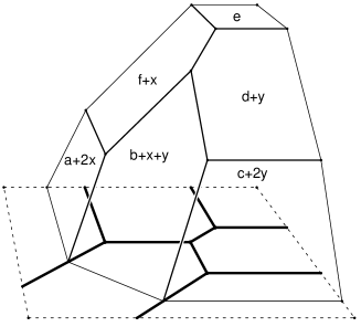
Figure 7. The graph of a piecewise linear concave function on $\mathbb{R}^{2}$.

Lemma 3.2.

If $F$ is a tropical polynomial then there exists a polynomial $f\in K[x_{1},\ldots,x_{n}]$ such that $\,\mathcal{T}(F)\,=\,\mathcal{T}(\langle f\rangle)$, and vice versa.

Proof.

If $F$ is the tropical polynomial (5) then we define

(6) $$f\quad=\quad\sum_{i=1}^{r}p_{i}(t)\cdot x_{1}^{a_{i1}}\cdots x_{n}^{a_{in}},$$

where $p_{i}(t)\in K$ is any Puiseux series of order $c_{i}$, for instance, $p_{i}(t)=t^{c_{i}}$. Since $\mathcal{G}=\{f\}$ is a tropical basis for its ideal, Theorem 2.6 implies $\,\mathcal{T}(F)\,=\,\mathcal{T}(\langle f\rangle)$. Conversely, given any polynomial $f$ we can define a tropical polynomial $F$ defining the same tropical hypersurface in $\mathbb{R}^{n}$ by setting $c_{i}={\rm order}(p_{i}(t))$. ∎

Theorem 3.3.

Every purely $(n-1)$-dimensional tropical variety in $\mathbb{R}^{n}$ is a tropical hypersurface and hence equals $\mathcal{T}(F)$ for some tropical polynomial $F$.

Proof.

Let $X=\mathcal{T}(I)$ be a tropical variety of pure dimension $n-1$ in $\mathbb{R}^{n}$. This means that every maximal face of the polyhedral complex is a convex polyhedron of dimension $n-1$. If $P_{1},\ldots,P_{s}$ are the minimal primes of the ideal $I$ then

$$X\quad=\quad\mathcal{T}(P_{1})\,\cup\,\mathcal{T}(P_{2})\,\cup\,\cdots\,\cup\mathcal{T}(P_{s}).$$

Each $\mathcal{T}(P_{i})$ is pure of codimension $1$, hence Theorem 2.7 implies that $P_{i}$ is a codimension $1$ prime in the polynomial ring $K[x_{1},\ldots,x_{n}]$. The prime ideal $P_{i}$ is generated by a single irreducible polynomial, $\,P_{i}=\langle f_{i}\rangle$. If we set $f=f_{1}f_{2}\cdots f_{s}$ then $\,X=\mathcal{T}(\langle f\rangle)$, and Lemma 3.2 gives the desired conclusion. ∎

Theorem 3.3 states that every tropical hypersurface in $\mathbb{R}^{n}$ has an elementary construction as the locus where a piecewise linear concave function fails to be linear. Tropical hypersurfaces in $\mathbb{TP}^{n-1}$ arise in the same manner from homogeneous tropical polynomials (5), where $\,a_{i1}+\cdots+a_{in}\,$ is the same for all $i$. We next describe this elementary construction for some curves in $\mathbb{TP}^{2}$ and some surfaces in $\mathbb{TP}^{3}$.

Example 3.4.

Quadratic curves in the plane are defined by tropical quadrics

$$F\,\,\,=\,\,\,a_{1}\odot x\odot x\,\,\oplus\,\,a_{2}\odot x\odot y\,\,\oplus\,\,a_{3}\odot y\odot y\,\,\oplus\,\,a_{4}\odot y\odot z\,\,\oplus\,\,a_{5}\odot z\odot z\,\,\oplus\,\,a_{6}\odot x\odot z.$$

The curve $\mathcal{T}(F)$ is a graph which has six unbounded edges and at most three bounded edges. The unbounded edges are pairs of parallel half rays in the three coordinate directions. The number of bounded edges depends on the $3\times 3$-matrix

(7) $$\begin{pmatrix}a_{1}&a_{2}&a_{6}\\ a_{2}&a_{3}&a_{4}\\ a_{6}&a_{4}&a_{5}\end{pmatrix}\,.$$

We regard the row vectors of this matrix as three points in $\mathbb{TP}^{2}$. If all three points are identical then $\mathcal{T}(F)$ is a tropical line counted with multiplicity two. If the three points lie on a tropical line then $\mathcal{T}(F)$ is the union of two tropical lines. Here the number of bounded edges of $\mathcal{T}(F)$ is two. In the general situation, the three points do not lie on a tropical line. Up to symmetry, there are five such general cases:

Case a: $\mathcal{T}(F)$ looks like a tropical line of multiplicity two (depicted in Figure 8 a)). This happens if and only if

$$2a_{2}\,\geq\,a_{1}+a_{3}\quad\hbox{and}\quad 2a_{4}\,\geq\,a_{3}+a_{5}\quad\hbox{and}\quad 2a_{6}\geq\,a_{1}+a_{5}\,.$$

Case b: $\mathcal{T}(F)$ has two double half rays: There are three symmetric possibilities. The one in Figure 8 b) occurs if and only if

$$2a_{2}\,\geq\,a_{1}+a_{3}\quad\hbox{and}\quad 2a_{4}\,\geq\,a_{3}+a_{5}\quad\hbox{and}\quad 2a_{6}\,<\,a_{1}+a_{5}\,.$$

Case c: $\mathcal{T}(F)$ has one double half ray: The double half ray is emanating in the $y$-direction if and only if

$$2a_{2}\,<\,a_{1}+a_{3}\quad\hbox{and}\quad 2a_{4}\,<\,a_{3}+a_{5}\quad\hbox{and}\quad 2a_{6}\,\geq\,a_{1}+a_{5}\,.$$

Figure 8 c) depicts the two combinatorial types for this situation. They are distinguished by whether $\,2a_{2}+a_{5}-a_{1}-2a_{4}\,$ is negative or positive.

$$\begin{array}[]{c@{\;}c@{\;}c@{}c}\includegraphics[width=79.6678pt]{pictures/ConicTypes1.eps}&\includegraphics[width=79.6678pt]{pictures/ConicTypes2.eps}&\includegraphics[width=79.6678pt]{pictures/ConicTypes3.eps}&\includegraphics[width=79.6678pt]{pictures/ConicTypes4.eps}\\ \text{a)}&\text{b)}&\lx@intercol\hfil\text{c)}\hfil\lx@intercol\end{array}$$

Figure 8. Types of non-proper tropical conics in $\mathbb{TP}^{2}$.

Case d: $\mathcal{T}(F)$ has one vertex not on any half ray. This happens if and only if

$$a_{2}+a_{4}\,<\,a_{3}+a_{6}\quad\hbox{and}\quad a_{2}+a_{6}\,<\,a_{1}+a_{4}\quad\hbox{and}\quad a_{4}+a_{6}\,<\,a_{2}+a_{5}\,.$$

If one of these inequalities becomes an equation, then $\mathcal{T}(F)$ is a union of two lines.

Case e: $\mathcal{T}(F)$ has four vertices and each of them lies on some half ray. Algebraically,

$$2a_{2}\,<\,a_{1}+a_{3}\quad\hbox{and}\quad 2a_{4}\,<\,a_{3}+a_{5}\quad\hbox{and}\quad 2a_{6}<\,a_{1}+a_{5}$$

and $$(a_{2}+a_{4}\,>\,a_{3}+a_{6}\quad\hbox{or}\quad a_{2}+a_{6}\,>\,a_{1}+a_{4}\quad\hbox{or}\quad a_{4}+a_{6}\,>\,a_{2}+a_{5})\,.$$

$$\begin{array}[]{c@{\quad}c@{\quad}c@{\quad}c}\lx@intercol\hfil\includegraphics[width=136.5733pt]{pictures/ConicTypes5.eps}\hfil\lx@intercol&\lx@intercol\hfil\includegraphics[width=136.5733pt]{pictures/ConicTypes6.eps}\hfil\lx@intercol\\ \lx@intercol\hfil\text{d)}\hfil\qquad&\lx@intercol\hfil\text{e)}\hfil\lx@intercol\end{array}$$

Figure 9. Types of proper tropical conics in $\mathbb{TP}^{2}$.

The curves in cases d) and e) are called proper conics. They are shown in Figure 9. The set of proper conics forms a polyhedral cone. Its closure in $\mathbb{TP}^{5}$ is called the cone of proper conics. This cone is defined by the three inequalities

(8) $$2a_{2}\,\leq\,a_{1}+a_{3}\quad\hbox{and}\quad 2a_{4}\,\leq\,a_{3}+a_{5}\quad\hbox{and}\quad 2a_{6}\leq\,a_{1}+a_{5}\,.$$

We will see later that proper conics play a special role in interpolation. ∎

We next describe arbitrary curves in the tropical plane $\mathbb{TP}^{2}$. Let $\mathcal{A}$ be a subset of $\,\{(i,j,k)\in\mathbb{N}_{0}^{3}\,:\,i+j+k=d\}$ for some $d$ and consider a tropical polynomial

(9) $$F(x,y,z)\quad=\ \sum_{(i,j,k)\in\mathcal{A}}a_{ijk}\odot x^{i}\odot y^{j}\odot z^{k}\,,\qquad\text{where $a_{ijk}\in\mathbb{R}$.}$$

Then $\mathcal{T}(F)$ is a tropical curve in the tropical projective plane $\mathbb{TP}^{2}$, and Theorem 3.3 implies that every tropical curve in $\mathbb{TP}^{2}$ has the form $\mathcal{T}(F)$ for some $F$.

Here is an algorithm for drawing the curve $\mathcal{T}(F)$ in the plane. The input to this algorithm is the support $\mathcal{A}$ and the list of coefficients $a_{ijk}$. For any pair of points $(i^{\prime},j^{\prime},k^{\prime}),(i^{\prime\prime},j^{\prime\prime},k^{\prime\prime})\in\mathcal{A}$, consider the system of linear inequalities

$$a_{i^{\prime}j^{\prime}k^{\prime}}+i^{\prime}x+j^{\prime}y+k^{\prime}z\ =\ a_{i^{\prime\prime}j^{\prime\prime}k^{\prime\prime}}+i^{\prime\prime}x+j^{\prime\prime}y+k^{\prime\prime}z$$

$$\qquad\qquad\qquad\qquad\qquad\qquad\leq a_{ijk}+ix+jy+kz\qquad\text{for }(i,j,k)\in\mathcal{A}\,.$$

The solution set to this system is either empty or a point or a segment or a ray in $\mathbb{TP}^{2}$. The tropical curve $\mathcal{T}(F)$ is the union of these segments and rays.

It appears as if the running time of this procedure is quadratic in the cardinality of $\mathcal{A}$, as we are considering arbitrary pairs of points $(i^{\prime},j^{\prime},k^{\prime})$ and $(i^{\prime\prime},j^{\prime\prime},k^{\prime\prime})$ in $\mathcal{A}$. However, most of these pairs can be ruled out a priori. The following refined algorithm runs in time $O(m\log m)$ where $m$ is the cardinality of $\mathcal{A}$. Compute the convex hull of the points $(i,j,k,a_{ijk})$. This is a three-dimensional polytope. The lower faces of this polytope project bijectively onto the convex hull of $\mathcal{A}$ under deleting the last coordinate. This defines a regular subdivision $\Delta$ of $\mathcal{A}$. A pair of vertices $(i^{\prime},j^{\prime},k^{\prime})$ and $(i^{\prime\prime},j^{\prime\prime},k^{\prime\prime})$ needs to be considered if and only if they form an edge in the regular subdivision $\Delta$. The segments of $\mathcal{T}(F)$ arise from the interior edges of $\Delta$, and the rays of $\mathcal{T}(F)$ arise from the boundary edges of $\Delta$. This shows:

Proposition 3.5.

The tropical curve $\mathcal{T}(F)$ is an embedded graph in $\mathbb{TP}^{2}$ which is dual to the regular subdivision $\Delta$ of the support $\mathcal{A}$ of the tropical polynomial $F$. Corresponding edges of $\mathcal{T}(F)$ and $\Delta$ are perpendicular.

If the coefficients of $F$ in (9) are sufficiently generic then the subdivision $\Delta$ is a regular triangulation. This means that the curve $\mathcal{T}(F)$ is a trivalent graph.

$$\begin{array}[]{c@{\qquad}c}\includegraphics[width=142.26378pt]{pictures/CJ1.eps}&\includegraphics[width=142.26378pt]{pictures/CJ3.eps}\\[14.22636pt] \includegraphics[width=71.13188pt]{pictures/CJ2.eps}&\includegraphics[width=71.13188pt]{pictures/CJ4.eps}\\ \end{array}$$

Figure 10. Tropical biquadratic curves.

Figure 10 shows two tropical curves whose support is a square with side length two. In both cases, the corresponding subdivision $\Delta$ is drawn below the curve $\mathcal{T}(F)$. These are tropical versions of biquadratic curves in $\mathbb{P}^{1}\times\mathbb{P}^{1}$, so they represent families of elliptic curves over $K$. The unique cycle in $\mathcal{T}(F)$ arises from the interior vertex of $\Delta$. The same construction yields tropical Calabi-Yau hypersurfaces in all dimensions.

All the edges in a tropical curve $\mathcal{T}(F)$ have a natural multiplicity, which is the lattice length of the corresponding edge in $\Delta$. In our algorithm, the multiplicity is computed as the greatest common divisor of $\,i^{\prime}-i^{\prime\prime}$, $j^{\prime}-j^{\prime\prime}$ and $k^{\prime}-k^{\prime\prime}$. Let $p$ be any vertex of the tropical curve $\mathcal{T}(F)$, let $v_{1},v_{2},\ldots,v_{r}$ be the primitive lattice vectors in the directions of the edges emanating from $p$, and let $m_{1},m_{2},\ldots,m_{r}$ be the multiplicities of these edges. Then the following equilibrium condition holds:

(10) $$m_{1}\cdot v_{1}\,+\,m_{2}\cdot v_{2}\,+\,\cdots\,+\,m_{r}\cdot v_{r}\quad=\quad 0.$$

The validity of this identity can be seen by considering the convex $r$-gon dual to $p$ in the subdivision $\Delta$. The edges of this $r$-gon are obtained from the vectors $m_{i}\cdot v_{i}$ by a $90$ degree rotation. But, clearly, the edges of a convex polygon sum to zero.

Our next theorem states that this equilibrium condition actually characterizes tropical curves in $\mathbb{TP}^{2}$. This remarkable fact provides an alternative definition of tropical curves. A subset $\Gamma$ of $\mathbb{TP}^{2}$ is a rational graph if $\Gamma$ is a finite union of rays and segments whose endpoints and directions have coordinates in the rational numbers $\mathbb{Q}$, and each ray or segment has a positive integral multiplicity. A rational graph $\Gamma$ is said to be balanced if the condition (10) holds at each vertex $p$ of $\Gamma$.

Theorem 3.6.

The tropical curves in $\mathbb{TP}^{2}$ are the balanced rational graphs.

Proof.

We have shown that every tropical curve is a balanced rational graph. For the converse, suppose that $\Gamma$ is any rational graph which is balanced. Considering the connected components of $\Gamma$ separately, we can assume that $\Gamma$ is connected. By a theorem of Crapo and Whiteley ([crapo-whiteley-82], see also [richter-gebert-b96, Section 13.1]), the balanced graph $\Gamma$ is the projection of the lower edges of a convex polytope. The rationality of $\Gamma$ ensures that we can choose this polytope to be rational. Its defining inequalities have the form $ix+jy+kz\geq a_{ijk}$ for some real numbers $a_{ijk}$. Now define a tropical polynomial $F$ as in (5). Then our algorithm implies that $\Gamma$ equals $\mathcal{T}(F)$. Theorem 3.3 completes the proof. ∎

Our polyhedral construction of curves can be generalized to hypersurfaces in tropical projective space $\mathbb{TP}^{n-1}$. This raises the question whether the class of all tropical varieties has a similar characterization. If so, then perhaps the algebraic introduction in Section 2 was irrelevant?  We wish to argue that this is most certainly not the case. Here is the crucial definition. A subset of $\mathbb{R}^{n}$ or $\mathbb{TP}^{n-1}$ is a tropical prevariety if it is the intersection of finitely many tropical hypersurfaces $\mathcal{T}(F)$.

Lemma 3.7.

Every tropical variety is a tropical prevariety, but not conversely.

Proof.

By Theorem 2.6 and Theorem 3.3, every tropical variety is a finite intersection of tropical hypersurfaces, arising from the polynomials in a tropical basis. But there are many examples of tropical prevarieties which are not tropical varieties. Consider the tropical lines $\mathcal{T}(L)$ and $\mathcal{T}(L^{\prime})$ where

$$L\,\,=\,\,0\odot x\,\,\oplus\,\,0\odot y\,\,\oplus\,\,0\odot z\quad\hbox{and}\quad L^{\prime}\,\,=\,\,0\odot x\,\,\oplus\,\,0\odot y\,\,\oplus\,\,1\odot z\,.$$

Then $\,\mathcal{T}(L)\,\cap\,\mathcal{T}(L^{\prime})\,$ is the half ray consisting of all points $(a,a,0)$ with $a\leq 0$. Such a half ray is not a tropical variety. ∎

When performing constructions in tropical algebraic geometry, it appears to be crucial that we work with tropical varieties and not just with tropical prevarieties. The distinction between these two categories is very subtle, with the algebraic notion of a tropical basis providing the key. In order for a tropical prevariety to be a tropical variety, the defining tropical hypersurfaces must obey some strong combinatorial consistency conditions, namely, those present among the Newton polytopes of some polynomials which form a tropical basis.

Synthetic constructions of families of tropical varieties that are not hypersurfaces require great care. The simplest case is that of lines in projective space $\mathbb{TP}^{n-1}$.

Example 3.8.

A line in $\mathbb{TP}^{n-1}$ is an embedded tree whose edges are either bounded line segments or unbounded half rays, subject to the following three rules:

1. The directions of all edges in the tree are spanned by integer vectors.

2. There are precisely $n$ unbounded half rays. Their directions are the $n$ standard coordinate directions $e_{1},\ldots,e_{n}$ in $\mathbb{TP}^{n-1}$.

3. If $u_{1},u_{2},\ldots,u_{r}$ are the primitive integer vectors in the directions of all outgoing edges at any fixed vertex of the tree then $u_{1}+u_{2}+\cdots+u_{r}=0$.

The correctness of this description follows from the results on tropical Grassmannians in [speyer-sturmfels-2003]. We refer to this article for details on tropical linear spaces.

4. Bézout’s Theorem

In classical projective geometry, Bézout’s Theorem states that the number of intersection points of two general curves in the complex projective plane is the product of the degrees of the curves. In this section we prove the same theorem for tropical geometry. The first step is to clarify what we mean by a curve of degree $d$.

A tropical polynomial $F$ as in (9) is said to be a tropical polynomial of degree $d$ if its support $\mathcal{A}$ is equal to the set $\{(i,j,k)\in\mathbb{N}_{0}^{3}\,:\,i+j+k=d\}$. Here the coefficients $a_{ijk}$ can be any real numbers, including $0$. Changing a coefficient $a_{ijk}$ to $0$ does not alter the support of a polynomial. After all, $0$ is the neutral element for multiplication $\odot$ and not for addition $\oplus$. Deleting a term from the polynomial $F$ and thereby shrinking its support corresponds to changing $a_{ijk}$ to $+\infty$. If $F$ is a tropical polynomial of degree $d$ then we call $\mathcal{T}(F)$ a tropical curve of degree $d$.

Example 4.1.

Let $d=2$ and consider the following tropical polynomials:

$$F_{1} = 3x^{2}\,\oplus\,5xy\,\oplus\,7y^{2}\,\oplus\,11xz\,\oplus\,13yz\,\oplus\,17z^{2},$$

$$F_{2} = 3x^{2}\,\oplus\,5xy\,\oplus\,7y^{2}\,\oplus\,11xz\,\oplus\,13yz\,\oplus\,0z^{2},$$

$$F_{3} = 0x^{2}\,\oplus\,0xy\,\oplus\,0y^{2}\,\oplus\,0xz\,\oplus\,0yz\,\oplus\,0z^{2},$$

$$F_{4} = 3x^{2}\,\oplus\,5xy\,\oplus\,7y^{2}\,\oplus\,11xz\,\oplus\,13yz\,\oplus\,(+\infty)z^{2},$$

$$F_{5} = 3x^{2}\,\oplus\,5xy\,\oplus\,7y^{2}\,\oplus\,11xz\,\oplus\,13yz.$$

$\mathcal{T}(F_{1})$, $\mathcal{T}(F_{2})$ and $\mathcal{T}(F_{3})$ are tropical curves of degree $2$. $\mathcal{T}(F_{4})=\mathcal{T}(F_{5})$ is a tropical curve, but it does not have a degree $d$. Can you draw these curves ? ∎

In order to state Bézout’s Theorem, we need to define intersection multiplicities for two balanced rational graphs in $\mathbb{TP}^{2}$. Consider two intersecting line segments with rational slopes, where the segments have multiplicities $m_{1}$ and $m_{2}$ and where the primitive direction vectors are $(u_{1},u_{2},u_{3}),(v_{1},v_{2},v_{3})\in\mathbb{Z}^{3}/\mathbb{Z}(1,1,1)$. Since the line segments are not parallel, the following determinant is nonzero:

$$\det\left(\begin{array}[]{ccc}u_{1}&u_{2}&u_{3}\\ v_{1}&v_{2}&v_{3}\\ 1&1&1\end{array}\right)$$

The (tropical) multiplicity of the intersection point is defined as the absolute value of this determinant times $m_{1}$ times $m_{2}$.

Theorem 4.2.

Consider two tropical curves $C$ and $D$ of degrees $c$ and $d$ in the tropical projective plane $\mathbb{TP}^{2}$. If the two curves intersect in finitely many points then the number of intersection points, counting multiplicities, is equal to $\,c\cdot d$.

            

Figure 11. Non-transversal intersection of a line and a conic.

We say that the curves $C$ and $D$ intersect transversally if each intersection point lies in the relative interior of an edge of $C$ and in the relative interior of an edge of $D$. Theorem 4.2 is now properly stated for the case of transversal intersections. Figure 11 shows a non-transversal intersection of a tropical conic with a tropical line. In the left picture a slight perturbation of the situation is shown. It shows that the point of intersection really comes from two points of intersection and has to be counted with the multiplicity that is the sum of the two points in the nearby situation. We will first give the proof of Bézout’s Theorem for the transversal case, and subsequently we will discuss the case of non-transversal intersections.

Proof.

The statement holds for curves in special position for which all intersection points occur among the half rays of the first curve in $x$-direction and the half rays of the second curve in $y$-direction. Such a position is shown in Figure 12.

Figure 12. Two conics intersect in four points.

The following homotopy moves any instance of two transversally intersecting curves to such a special situation. We fix the first curve $C$ and we translate the second curve $D$ with constant velocity along a sufficiently general piecewise linear path. Let $D_{t}$ denote the curve $D$ at time $t\geq 0$. We can assume that for no value of $t$ a vertex of $C$ coincides with a vertex of $D_{t}$ and that for all but finitely many values of $t$ the two curves $C$ and $D_{t}$ intersect transversally. Suppose these special values of $t$ are the time stamps $t_{1}<t_{2}<\cdots<t_{r}$. For any value of $t$ strictly between two successive time stamps $t_{i}$ and $t_{i+1}$, the number of intersection points in $\,C\,\cap\,D_{t}\,$ remains unchanged, and so does the multiplicity of each intersection point. We claim that the total intersection number also remains unchanged across a time stamp $t_{i}$.

Let $P$ be the set of branching points of $C$ which are also contained in $D_{t_{i}}$ and the set of branching points of $D_{t_{i}}$ which are also contained in $C$. Since $P$ is finite it suffices to show the invariance of intersection multiplicity for any point $p\in P$. Either $p$ is a vertex of $C$ and lies in the relative interior of a segment of $D_{t_{i}}$, or $p$ is a vertex of $D_{t_{i}}$ and lies in the relative interior of a line segment of $C$. The two cases are symmetric, so we may assume that $p$ is a vertex of $D_{t_{i}}$ and lies in the relative interior of a segment $S$ of $C$. Let $\ell$ be the line underlying $S$ and $u$ be the weighted outgoing direction vector of $p$ along $\ell$. Further let $v^{(1)},\ldots,v^{(k)}$ and $w^{(1)},\ldots,w^{(l)}$ be the weighted direction vectors of the outgoing edges of $p$ into the two open half planes defined by $\ell$. At an infinitesimal time $t$ before and after $t_{i}$ the total intersection multiplicities at the neighborhoods of $p$ are

$$m^{\prime}=\sum_{i=1}^{k}\left|\det\left(\begin{array}[]{ccc}u_{1}&u_{2}&u_{3}\\ v^{(i)}_{1}&v^{(i)}_{2}&v^{(i)}_{3}\\ 1&1&1\end{array}\right)\right|\;\text{ and }\;m^{\prime\prime}=\sum_{j=1}^{l}\left|\det\left(\begin{array}[]{ccc}u_{1}&u_{2}&u_{3}\\ w^{(j)}_{1}&w^{(j)}_{2}&w^{(j)}_{3}\\ 1&1&1\end{array}\right)\right|.$$

Since within each of the two sums the determinants have the same sign, equality of $m^{\prime}$ and $m^{\prime\prime}$ follows immediately from the equilibrium condition at $p$.

In case of a non-transversal intersection, the intersection multiplicity is the (well-defined) multiplicity of any perturbation in which all intersections are transversal (see Figure 11). The validity of this definition and the correctness of Bézout’s theorem now follows from our previous proof for the transversal case. ∎

The statement of Bézout’s Theorem is also valid for the intersection of $n-1$ tropical hypersurfaces of degrees $d_{1},d_{2},\ldots,d_{n-1}$ in $\mathbb{TP}^{n-1}$. If they intersect in finitely many points, then the number of these points (counting multiplicities) is always $\,d_{1}d_{2}\cdots d_{n-1}$. Moreover, also Bernstein’s Theorem for sparse systems of polynomial equations remains valid in the tropical setting. This theorem states that the number of intersection points always equals the mixed volume of the Newton polytopes. For a discussion of the tropical Bernstein Theorem see [SSPE, Section 9.1].

Families of tropical complete intersections have an important feature which is not familiar from the classical situation, namely, intersections can be continued across the entire parameter space of coefficients. We explain this for the intersection of two curves $C$ and $D$ of degrees $c$ and $d$ in $\mathbb{TP}^{2}$. Suppose the (geometric) intersection of $C$ and $D$ is not finite. Pick any nearby curves $C_{\epsilon}$ and $D_{\epsilon}$ such that $C_{\epsilon}$ and $D_{\epsilon}$ intersect in finitely many points. Then $\,C_{\epsilon}\,\cap\,D_{\epsilon}\,$ has cardinality $cd$.

Theorem 4.3.

The limit of the point configuration $\,C_{\epsilon}\,\cap\,D_{\epsilon}\,$ is independent of the choice of perturbations. It is a well-defined subset of $cd$ points in $\,C\,\cap\,D$.

Of course, as always, we are counting multiplicities in the intersection $\,C_{\epsilon}\,\cap\,D_{\epsilon}\,$ and hence also in its limit as $\epsilon$ tends to $0$. This limit is a configuration of points with multiplicities, where the sum of all multiplicities is $cd$. We call this limit the stable intersection of the curves $C$ and $D$, and we denote this multiset of points by

$$C\,\cap_{st}D\quad=\quad\lim_{\epsilon\rightarrow 0}(C_{\epsilon}\,\cap\,D_{\epsilon}).$$

Hence we can strengthen the statement of Bézout’s Theorem as follows:

Corollary 4.4.

Any two curves of degrees $c$ and $d$ in the tropical projective plane $\mathbb{TP}^{2}$ intersect stably in a well-defined set of $cd$ points, counting multiplicities.

      

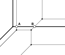
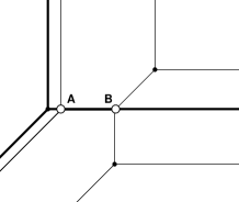
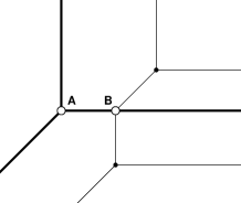
Figure 13. Stable intersections of a line and a conic.

The proof of Theorem 4.3 follows from our proof of the tropical Bézout’s Theorem. We shall illustrate the statement by two examples. Figure 13 shows the stable intersections of a line and a conic. In the first picture they intersect transversally in the points $A$ and $B$. In the second picture the line is moved to a position where the intersection is no longer transversal. The situation in the third picture is even more special. However, observe that for any nearby transversal situation the intersection points will be close to $A$ and $B$. In all three pictures, the pair of points $A$ and $B$ is the stable intersection of the line and the conic. In this manner we can construct a continuous piecewise linear map which maps any pair of conics to their four intersection points.

      

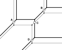
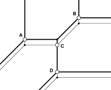
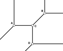
Figure 14. The stable intersection of a conic with itself.

Figure 14 illustrates another fascinating feature of stable intersections. It shows the intersection of a conic with a translate of itself in a sequence of three pictures. The points in the stable intersection are labeled $A,B,C,D$. Observe that in the third picture, where the conic is intersected with itself, the stable intersections coincide with the four vertices of the conic. The same works for all tropical hypersurfaces in all dimensions. The stable self-intersection of a tropical hypersurface in $\mathbb{TP}^{n-1}$ is its set of vertices, each counted with an appropriate multiplicity.

Our discussion suggests a general result to the effect that there is no monodromy in tropical geometry. It would be worthwhile to make this statement precise.

5. Solving linear equations using Cramer’s rule

We now consider the problem of intersecting $k$ tropical hyperplanes in $\mathbb{TP}^{n-1}$. If these hyperplanes are in general position then their intersection is a tropical linear space of dimension $n-k-1$. If they are in special position then their intersection is a tropical prevariety of dimension larger than $n-k-1$ but it is usually not a tropical variety. However, just like in the previous section, this prevariety always contains a well-defined stable intersection which is a tropical linear space of dimension $n-k-1$. The map which computes this stable intersection is nothing but Cramer’s Rule. The aim of this section is to make these statements precise and to outline their proofs.

Let $A=(a_{ij})$ be a $k\times k$-matrix with entries in $\mathbb{R}\cup\{+\infty\}$. We define the tropical determinant of $A$ by evaluating the expansion formula tropically:

$$\text{det}_{\text{trop}}(A)\,\,=\,\,\bigoplus_{\sigma\in S_{k}}(a_{1,\sigma_{1}}\odot\cdots\odot a_{k,\sigma_{k}})\,\,=\,\,\min_{\sigma\in S_{k}}(a_{1,\sigma_{1}}+\cdots+a_{k,\sigma_{k}})\,.$$

Here $S_{k}$ is the group of permutations of $\{1,2,\ldots,k\}$. The matrix $A$ is said to be tropically singular if this minimum is attained more than once. This is equivalent to saying that $A$ is in the tropical variety defined by the ordinary $k\times k$-determinant.

Lemma 5.1.

The matrix $A$ is tropically singular if and only if the $k$ points whose coordinates are the column vectors of $A$ lie on a tropical hyperplane in $\mathbb{TP}^{k-1}$.

Proof.

If $A$ is tropically singular then we can choose a $k\times k$-matrix $U(t)$ with entries in the field $K=\overline{\mathbb{Q}(t)}$ such that ${\rm det}(U(t))=0$ and ${\rm order}(U(t))=A$. There exists a non-zero vector $v(t)\in K^{n}$ in the kernel of $\,U(t)$. The identity $\,U(t)\cdot v(t)=0\,$ implies that the column vectors of $A$ lie on the tropical hyperplane $\,\mathcal{T}\bigl{(}v_{1}(t)\cdot x_{1}+\cdots+v_{n}(t)\cdot x_{n}\bigr{)}$. The converse direction follows analogously. ∎

The tropical determinant of a matrix is also known as the min-plus permanent. In tropical geometry, just like in algebraic geometry over a field of characteristic $2$, the determinant and the permanent are indistinguishable. In practice, one does not compute the tropical determinant of a $k\times k$-matrix by first computing all $k\,!$ sums $\,a_{1,\sigma_{1}}+\cdots+a_{k,\sigma_{k}}\,$ and then taking the minimum. This process would take exponential time in $k$. Instead, one recognizes this task as an assignment problem. A well-known result from combinatorial optimization [Schrijver, Corollary 17.4b] implies

Remark 5.2.

The tropical determinant of a $k\times k$-matrix can be computed in $O(k^{3})$ arithmetic operations.

Fix a $k\times n$-matrix $C=(c_{ij})$ with $k<n$. Each row gives a tropical linear form

$$F_{i}\quad=\quad c_{i1}\odot x_{1}\,\oplus\,c_{i2}\odot x_{2}\,\oplus\,\cdots\,\oplus c_{in}\odot x_{n}.$$

For any $k$-subset $I=\{i_{1},\ldots,i_{k}\}$ of $\{1,2,\ldots,n\}$, we let $C_{I}$ denote the $k\times k$-submatrix of $C$ with column indices $I$, and we abbreviate its tropical determinant

$$w_{I}\quad=\quad\text{det}_{\text{trop}}(C_{I}).$$

Let $J=\{j_{0},j_{1},\cdots,j_{n-k}\}$ be any $(n-k+1)$-subset of $\{1,\ldots,n\}$ and $J^{c}$ its complement. The following tropical linear form is a circuit of the $k\times n$-matrix $C$:

$$G_{J}\quad=\quad w_{J^{c}\cup\{j_{0}\}}\odot x_{j_{0}}\,\,\,\oplus\,\,\,w_{J^{c}\cup\{j_{1}\}}\odot x_{j_{1}}\,\,\,\oplus\,\,\,\cdots\,\,\,\oplus\,\,\,w_{J^{c}\cup\{j_{n-k}\}}\odot x_{j_{n-k}}.$$

We form the intersection of the $\binom{n}{k-1}$ tropical hyperplanes defined by the circuits:

(11) $$\bigcap_{1\leq j_{0}<j_{1}<\cdots<j_{k}\leq n}\,\,\,\mathcal{T}\bigl{(}G_{J}\bigr{)}\qquad\subset\quad\mathbb{TP}^{n-1}.$$

Similarly, we form the intersection of the $k$ tropical hyperplanes given by the rows:

(12) $$\mathcal{T}(F_{1})\,\,\cap\,\,\mathcal{T}(F_{2})\,\,\cap\,\,\cdots\,\,\cap\,\,\mathcal{T}(F_{k})\qquad\subset\quad\mathbb{TP}^{n-1}.$$

The problem of solving a system of $k$ tropical linear equations in $n$ unknowns is the same as computing the intersection (12). We saw in Section 3 that (12) is in general only a prevariety, even for $k=2$, $n=3$. In higher dimensions this prevariety can have maximal faces of different dimensions. The intersection (11) is much nicer. We show that it is the stable version of the poorly behaved intersection (12):

Theorem 5.3.

The intersection (11) is a tropical linear space of codimension $k$ in $\mathbb{TP}^{n-1}$. It is always contained in the prevariety (12). The two intersections are equal if and only if none of the $k\times k$-submatrices $\,C_{I}\,$ of $\,C\,$ is tropically singular.

Proof. Consider the vector $w\in\mathbb{R}^{\binom{n}{k}}$ whose coordinates are the tropical $k\times k$-determinants $w_{I}$. Then $w$ is a point on the tropical Grassmannian [speyer-sturmfels-2003]. By [speyer-sturmfels-2003, Theorem 3.8], the point $w$ represents a tropical linear space $L_{w}$ in $\mathbb{TP}^{n-1}$. The tropical linear space $L_{w}$ has codimension $k$, and it is precisely the set (11).

The second assertion follows from the if-direction in the third assertion. Indeed, if $C$ is any $k\times n$-matrix which has a tropically singular $k\times k$-submatrix then we can find a family of matrices $C^{(\epsilon)}$, $\epsilon>0$, with $\,{\rm lim}_{\epsilon\rightarrow 0}C^{(\epsilon)}\,=\,C\,$ such that each $C^{(\epsilon)}$ has all $k\times k$-matrices tropically non-singular. Let $w^{(\epsilon)}\in\mathbb{R}^{\binom{n}{k}}$ be the vector of tropical $k\times k$-subdeterminants of $C^{(\epsilon)}$. The tropical linear space $L_{w^{(\epsilon)}}$ depends continuously on the parameter $\epsilon$. If $x$ is any point in the plane $L_{w}$ then there exists a sequence of points $x^{(\epsilon)}\in L_{w^{(\epsilon)}}$ such that $\,{\rm lim}_{\epsilon\rightarrow 0}x^{(\epsilon)}\,=\,x$. Now consider the tropical linear form $\,F_{i}^{(\epsilon)}\,$ given by the $i$-th row of the matrix $C_{\epsilon}$. By the if-direction of the third assertion, the point $x^{(\epsilon)}$ lies in the tropical hypersurface $\mathcal{T}(F_{i}^{(\epsilon)})$. This hypersurface also depends continuously on $\epsilon$, and therefore we get the desired conclusion $x\in\mathcal{T}(F_{i})$ for all $i$.

We next prove the only if-direction in the third assertion. Suppose that the $k\times k$-matrix $C_{I}$ is tropically singular. By Lemma 5.1, there exists a vector $p\in\mathbb{R}^{k}$ in the tropical kernel of $C_{I}$. We can augment $p$ to a vector in the tropical kernel (12) of $C$ by placing any sufficiently large positive reals in the other $n-k$ coordinates. Hence the prevariety (12) contains a polyhedral cone of dimension $n-k$ in $\mathbb{TP}^{n-1}$.

What is left to prove at this point is the most difficult part of Theorem 5.3, namely, assuming that the $k\times k$-submatrices of $C$ are tropically non-singular then we must show that the tropical prevariety (12) is contained in the tropical linear space (11). We will now interrupt the general proof to give a detailed discussion of the special case $n=k+1$, when (11) and (12) consist of a single point in $\mathbb{TP}^{n-1}$. Thereafter we shall return to the third assertion in Theorem 5.3 for $n\geq k+2$. ∎

Let $C$ be a rational $(n-1)\times n$-matrix whose $n$ maximal square submatrices are tropically non-singular. We claim that the associated system of $n-1$ tropical linear equations in $n$ unknowns has a unique solution point $p$ in tropical projective space $\mathbb{TP}^{n-1}$. In the next two paragraphs, we shall explain how the results on linkage trees in [zelevinsky, Theorem 2.4] can be used to prove both this result and to devise a polynomial-time algorithm for computing the point $p$ from the matrix $C$.

Let $Y$ be an $(n-1)\times n$-matrix of indeterminates, and consider the problem of minimizing the dot product $C\cdot Y=\sum_{ij}c_{ij}y_{ij}$ subject to the constraints that $Y$ is non-negative, all its row sums are $n$ and all its column sums are $n-1$. This is a transportation problem which can be solved in polynomial time in the binary encoding of $C$. Our hypothesis that the maximal minors of $C$ are tropically non-singular means that $C$ specifies a coherent matching field. Theorem 2.8 in [zelevinsky] implies that the above transportation problem has a unique optimal solution $Y^{*}$. Each row of $Y^{*}$ has precisely two non-zero entries: this data specifies the linkage tree $T$ as in Theorem 2.4 of [zelevinsky]. Thus $T$ is a tree on the nodes $1,2,\ldots,n$ whose edges are labeled by $1,2,\ldots,n-1$. If the two non-zero entries of the $i$-th row of $Y^{*}$ are in columns $j_{i}$ and $k_{i}$ then $\{j_{i},k_{i}\}$ is the edge labeled by $i$. We claim that our desired point $p=(p_{1},\ldots,p_{n})$ satisfies the equations

(13) $$c_{ij_{i}}+p_{j_{i}}\,\,=\,\,c_{ik_{i}}+p_{k_{i}}\qquad i=1,2,\ldots,n-1.$$

Since $T$ is a tree, these equations have a unique solution $p$ which can be computed in polynomial time from $Y^{*}$ and hence from $C$. It remains to prove the claim that $p$ solves the tropical equations and is unique with this property.

We may assume without loss of generality that the zero vector $(0,0,\ldots,0)$ is a solution of the given tropical equations. We can change the given matrix $C$ by scalar addition in each column until each column is non-negative and has at least one zero entry. Then each row of $C$ is non-negative and has at least two zero entries. The objective function value of our transportation problem is zero, and the set of zero entries of $C$ supports a unique linkage tree $T$. Now our tropical linear system consists of the $n-1$ equations

$$p_{j_{i}}\,\,=\,\,p_{k_{i}}\qquad i=1,2,\ldots,n-1$$

and $(n-1)(n-2)$ inequalities $\,p_{j_{i}}\leq c_{ik}$, one for each position $(i,k)$ which is not in the matching field. The zero vector $p=(0,0,\ldots,0)$ is the unique solution to these equations and inequalities. This argument completes the proof of Theorem 5.3 for the case $n=k+1$. We summarize our discussion as follows.

Corollary 5.4.

Solving a system of $n\!-\!1$ tropical linear equations in $n$ unknowns amounts to computing the linkage tree of the coefficient matrix $C$. This can be done in polynomial time by solving the transportation problem with cost matrix $C$, row sums $n$ and column sums $n-1$. The solution $p$ is given by the system (13).

We note that the solution to the inhomogeneous square system of tropical linear equations $A\odot x=b$ presented in [olsder-roos-88] corresponds to a special linkage tree. This tree is a star with center indexed by $b$ and leaves indexed by the $n$ columns of $A$.

Proof of Theorem 5.3 (continued). We now sketch the proof of the if-direction in the third assertion for $n\geq k+2$. Suppose $C$ has no tropically singular $k\times k$-submatrix. We wish to show that if a point $x$ lies in (12) then it also lies in (11). Clearly, it suffices to show this for the zero vector $x=0$. Thus we will show: If $0$ is in (12) then it is in (11). After tropical scalar multiplication, we may assume that the coefficients $c_{i1},\ldots,c_{in}$ of $F_{i}$ are non-negative and their minimum is $0$. Since $0\in\mathcal{T}(F)$, this minimum is attained twice. At this stage, the $k\times n$-matrix $C$ is non-negative and each row contains at least two zero entries.

We next apply the combinatorial theory developed in [zelevinsky]. Our hypothesis states that the minimum in the definition of a tropical $k\times k$-subdeterminant of $C$ is uniquely attained. Thus it specifies a coherent matching field. Let $\Sigma$ be the support set of this matching field. It contains all the locations $(i,j)$ of zero entries of $C$. This means that the prevariety (12) remains unchanged if we replace all entries outside of $\Sigma$ by $+\infty$. Now, using the results in [zelevinsky, §4], we can transform our matrix $C$ by tropical row operations to an equivalent matrix $C^{\prime}$ whose rows are tropical $k\times k$-minors. The tropical linear forms $F^{\prime}_{i}$ given by the rows of that matrix $C^{\prime}$ are circuits. But they still have the same intersection (12). From the Support Theorem in [zelevinsky] we infer that this intersection has codimension $k$ locally around $x=0$. This holds for any point $x$ in the relative interior of any maximal face of the polyhedral complex (12), and therefore the complexes (12) and (11) are equal. ∎

We apply the Theorem 5.3 (with $n=6$) to study families of conics in the tropical projective plane $\mathbb{TP}^{2}$. The support set for conics is

$$\mathcal{A}\quad=\quad\bigl{\{}\,(2,0,0),\,(1,1,0),\,(0,2,0),\,(0,1,1),\,(0,0,2),\,(1,0,1)\,\bigr{\}}.$$

We identify points $\,a=(a_{1},a_{2},a_{3},a_{4},a_{5},a_{6})\,$ with tropical conics $\mathcal{T}(F)$ as in Example 3.4. Fix a configuration of points $P_{i}=(x_{i},y_{i},z_{i})\in\mathbb{TP}^{2}$ for $i=1,2,\ldots,k$. Let $C$ be the $k\times 6$-matrix whose row vectors are

$$(2x_{i},\,x_{i}+y_{i},\,2y_{i},\,y_{i}+z_{i},\,2z_{i},\,x_{i}+z_{i})\,,\quad 1\leq i\leq k\,.$$

Lemma 5.5.

The vector $a$ lies in the tropical kernel of the matrix $C$ if and only if the points $P_{1},P_{2},\ldots,P_{k}$ lie on the conics $\mathcal{T}(F)$.

The implications of Theorem 5.3 for $k=4$ constitute the subject of the next section. For $k=5$ we conclude the following results.

Corollary 5.6.

Any five points in $\mathbb{TP}^{2}$ lie on a conic. The conic is unique if and only if the points are not on a curve whose support is a proper subset of $\mathcal{A}$.

Figure 15. Conic through five points.

The unique conic through five general points is computed by Cramer’s rule from the matrix $C$, that is, the coefficient $a_{i}$ is the tropical $5\times 5$-determinant gotten from $C$ by deleting the $i$-th column. The remarkable fact is that the conic given by Cramer’s rule is stable, i.e., the unique conic through any perturbation of the given points will converge to that conic, in analogy to the discussion at the end of Section 4. It turns out that the stable conics given by quintuples of points in $\mathbb{TP}^{2}$ are always proper, that is, they belong to types (d) and (e) in Example 3.4.

Theorem 5.7.

The unique stable conic through any five given (not necessarily distinct) points is proper.

Proof.

For $\tau\in\{x^{2},xy,y^{2},xz,yz,z^{2}\}$ let $a_{\tau}$ denote the tropical $5\times 5$-subdeterminant of the $5\times 6$ coefficient matrix obtained by omitting the column associated with the term $\tau$. Since for any $x$ and $y$ we have

$$2\cdot\min\{2x,2y\}\ \leq\ \min\{2x,x+y\}+\min\{x+y,2y\}\,,$$

the definition of the tropical determinant implies

$$2a_{xy}\leq a_{x^{2}}+a_{y^{2}}\,,$$

and similarly

$$2a_{xz}\leq a_{x^{2}}+a_{z^{2}}\,,\quad 2a_{yz}\leq a_{y^{2}}+a_{z^{2}}\,.$$

This shows that the conic with these coefficients is proper. This proves our claim. ∎

We have implemented the computation of the stable conic through five given points into the geometry software Cinderella. The user clicks any five points with the mouse onto the computer screen. The program then sets up the corresponding $5\times 6$-matrix $C$, it computes the six tropical $5\times 5$-minors of $C$, and it then draws the curve onto the screen. This is done with the lifting method shown in Figure 7.

The presence of stability (i.e. the absence of monodromy) ensures that the software behaves smoothly and always produces the correct picture of the stable proper conic. For instance, if the user inputs the same point five times then Cinderella will correctly draw the double line (from case (a) of Example 3.4) with vertex at that point. Can you guess what happens if the user clicks one point twice and another point three times ?

6. Quadratic curves through four given points

In this section we study the set of tropical conics passing through four given points $P_{i}=(x_{i},y_{i},z_{i})\in\mathbb{TP}^{2}$, $1\leq i\leq 4$. By Theorem 5.3, if all $4\times 4$-submatrices of the $4\times 6$-matrix $C$ with rows

$$(2x_{i},\,x_{i}+y_{i},\,2y_{i},\,y_{i}+z_{i},\,2z_{i},\,x_{i}+z_{i})\,,\quad 1\leq i\leq 4\,,$$

are tropically nonsingular, then this set of conics is a tropical line in $\mathbb{TP}^{5}$. By Example 3.8 these are trees with six leaves. In the following we only consider quadruples of points which satisfy this genericity condition. We note that the pencil of conics contains several distinguished conics.

1. Three degenerate conics which are the pairs of two lines (see Figure 16).

         

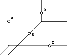
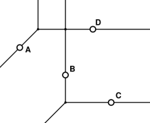
   Figure 16. Pairs of two lines through four given points

2. Conics in which one of the four points is a vertex of the conic (see Figure 17).

   $$\begin{array}[]{c@{\quad}c@{\quad}c@{\quad}c}\includegraphics[width=113.81102pt]{pictures/Conic8ng.eps}&\includegraphics[width=113.81102pt]{pictures/Conic3ng.eps}\\ \includegraphics[width=113.81102pt]{pictures/Conic16ng.eps}&\includegraphics[width=113.81102pt]{pictures/Conic4ng.eps}\end{array}$$

   Figure 17. One of the given points is a vertex of a conic.

3. Conics in which the coefficient of one term converges to $+\infty$. Figure 18 shows the limits of these conics. Geometrically, the tentacle of the conic associated with the distinguished term is missing. Note that conics of that type have only three internal vertices.

   $$\begin{array}[]{c@{\qquad}c@{\qquad}c}\includegraphics[width=93.89418pt]{pictures/Conic10ng.eps}&\includegraphics[width=93.89418pt]{pictures/Conic21ng.eps}&\includegraphics[width=93.89418pt]{pictures/Conic22ng.eps}\\[4.30554pt] \includegraphics[width=93.89418pt]{pictures/Conic17ng.eps}&\includegraphics[width=93.89418pt]{pictures/Conic6ng.eps}&\includegraphics[width=93.89418pt]{pictures/Conic24ng.eps}\end{array}$$

   Figure 18. The six limits conics through four given points

Figure 19 depicts the tree of conics through the four points $(0,6,0)$, $(5,3,0)$, $(10,0,0)$, $(8,8,0)$. The six leaves are the limit conics in Figure 18.

Figure 19. The tree of conics through four given points

Hence, the combinatorial type of a pencil of conics is described by a tree with six labeled leaves $x^{2},xy,y^{2},yz,z^{2},xz$ and four trivalent (unlabeled) internal vertices. Since the number of trivalent trees with $n$ labeled leaves is the Schröder number

$$(2n-5)!!=(2n-5)\cdot(2n-7)\cdots 5\cdot 3\cdot 1\,,$$

there are at most 105 different combinatorial types of pencil of conics. These 105 trees come in two symmetry classes:

Caterpillar trees:

There are 90 trees in which each of the four vertices is adjacent to at least one half ray (such as the tree in Figure 19).

Snowflake trees:

There are 15 trees in which there exists one vertex which is not adjacent to any half ray.

We say that a tree $\Gamma$ is realizable by a pencil of conics if there exists a configuration of four points in $\mathbb{TP}^{2}$ whose pencil of conics gives the tree $\Gamma$. The following statements characterize which of the 105 trees are realizable.

Theorem 6.1.

A tree $\Gamma$ is realizable if and only if $\Gamma$ can be embedded as a planar graph into the unit disc such that the six labeled vertices are located in the cyclic order $x^{2},xy,y^{2},yz,z^{2},zx$ on the boundary of the disc.

Corollary 6.2.

Exactly 14 of the 105 trees are realizable. Twelve of them are caterpillar trees and two of them are snowflake trees.

Figure 20 shows one of the realizable caterpillar trees and one of the realizable snowflake trees. In particular, the statement shows that a snowflake tree can be obtained as the complete intersection of four tropical hyperplanes in $\mathbb{TP}^{5}$. By Example 6.2 in [speyer-sturmfels-2003]), the tropical $3$-plane in $\mathbb{TP}^{5}$ which is dual to the snowflake tree is not a complete intersection.

      

Figure 20. A realizable caterpillar and a realizable snowflake

In order to prove Theorem 6.1, we consider the following more general setting. Let $\mathcal{A}=\{a_{1},a_{2},\ldots,a_{n}\}$ be an $n$-element subset of $\{(i,j,k)\in\mathbb{N}_{0}^{3}:i+j+k=d\}$ for some $d$. Consider a tree $\Gamma$ with $n$ leaves which are labeled by the elements of $\mathcal{A}$. The combinatorial type of the tree $\Gamma$ is specified by the induced subtrees on four leaves $\{a_{i},a_{j},a_{k},a_{l}\}$. The four possible subtrees are denoted as follows:

$$(ij|kl)\,,\,\,(ik|jl)\,,\,\,(il|jk)\,,\,\,(ijkl).$$

The first three trees are the trivalent trees on $i,j,k,l$ and the last tree is the tree with one $4$-valent node. We say that $\Gamma$ is compatible with $\mathcal{A}$ if the following condition holds: if $(ij|kl)$ is a trivalent subtree of $\Gamma$, then the convex hull of $a_{i},a_{j},a_{k}$, and $a_{l}$ has at least one of the segments ${\rm conv}(a_{i},a_{j})$ or ${\rm conv}(a_{k},a_{l})$ as an edge.

The space of curves with support $\mathcal{A}$ is identified with the tropical projective space $\mathbb{TP}^{n-1}$. Now consider a configuration $C$ of $n-2$ points in $\mathbb{TP}^{2}$ which does not lie on any tropical curve with support $\mathcal{A}\backslash\{a_{i},a_{j}\}$ for any pair $i,j$. Then the set of all curves with support $\mathcal{A}$ which pass through $C$ is a tropical line $\Gamma_{C}$ in $\mathbb{TP}^{n-1}$. Combinatorially, the line $\Gamma_{C}$ is a tree whose leaves are labeled by $\mathcal{A}$.

Theorem 6.3.

For every configuration $C$, the tree $\Gamma_{C}$ is compatible with $\mathcal{A}$.

Proof.

The theorem is trivial for $n\leq 3$. In the case $n=4$, it is proved by examining all combinatorial types of four-element-configurations of $\mathcal{A}$ and two-point configurations in the plane. This involves an exhaustive case analysis which we omit here. For the general case $n\geq 5$, we assume by induction that the result is already known for $n-1$.

The Plücker coordinate $p_{ij}$ of the line $\Gamma_{C}$ is the tropical determinant of the $(n-2)\times(n-2)$-matrix whose rows are labeled by $C$, whose columns are labeled by $\mathcal{A}\backslash\{a_{i},a_{j}\}$ and whose entries are the dot products of the row labels with the column labels. Fix any quadruple $ijkl$ and consider the restricted Plücker vector

$$P\quad=\quad(p_{ij},p_{ik},p_{il},p_{jk},p_{jl},p_{kl}).$$

Supposing that $n\not\in\{i,j,k,l\}$, we can compute these six tropical $(n-2)\times(n-2)$-determinants by tropical Laplace expansion with respect to the last row $n$:

$$P\quad=\quad\bigoplus_{c\in C}\,(a_{n}\cdot c)\odot(p_{ij}^{(c)},p_{ik}^{(c)},p_{il}^{(c)},p_{jk}^{(c)},p_{jl}^{(c)},p_{kl}^{(c)}).$$

Here $p_{ij}^{(c)}$ is the tropical $(n-3)\times(n-3)$-minor gotten from the matrix for $p_{ij}$ by deleting column $n$ and row $c$. Each of the Plücker vectors in this sum defines a tree which is compatible with the set $\{a_{i},a_{j},a_{k},a_{l}\}$, since $\Gamma_{C\backslash\{c\}}$ is compatible with $\mathcal{A}\backslash\{a_{n}\}$ by induction. The proof now follows from a lemma to the effect a tropical linear combination of compatible Plücker vectors is always compatible. ∎

Corollary 6.4.

If ${\rm conv}(\mathcal{A})$ is a convex polygon which has $a_{1},a_{2},\ldots,a_{n}$ on its boundary, then the compatible trees are precisely the planar trees whose leaves form an $n$-gon. The number of compatible trees is the Catalan number $\,\frac{1}{n-1}\binom{2n-4}{n-2}$.

We do not know whether every tree $\Gamma$ which is compatible with $\mathcal{A}$ can be realized as $\Gamma=\Gamma_{C}$ by some configuration $C$ of $n-2$ points in $\mathbb{TP}^{2}$. For the special case

$$\mathcal{A}\quad=\quad\bigl{\{}\,(2,0,0),\,(1,1,0),\,(0,2,0),\,(0,1,1),\,(0,0,2),\,(1,0,1)\,\bigr{\}},$$

there are $14$ compatible trees, by Corollary 6.4, and we checked that each of them is realizable. This proves Theorem 6.1 and Corollary 6.2 on quadratic curves through four given points.

7. Incidence Theorems and Tropical Cinderella

The previous sections showed that central concepts of classical projective geometry (such as intersection multiplicities, Bézout’s and Bernstein’s Theorem, as well as determinants) can be transferred to tropical geometry. In this section, we report on first insights on the question in how far projective incidence theorems carry over to the tropical world. By pointing out some pitfalls, we would like to argue that these generalizations require great care.

Our investigations were supported by a prototype of a tropical version of the dynamic geometry software Cinderella [CINDERELLA] (most pictures in this article were generated with this tool). This software supports the interactive manipulation of elementary geometric constructions. Here, an elementary geometric construction is considered as a construction sequence that starts with a set of free elements (e.g., points) and proceeds by constructively adding new dependent elements (e.g., the line passing through two points, intersection points of two lines, conics through five points). Once a construction is finished, one can explore its dynamic behavior by simply dragging the free elements. The dependent elements move according to the construction sequence. Our experimental version of this software provides basic operations for join (i.e., the line passing through two points), meet (i.e., the intersection point of two lines) and the stable conic through five points in $\mathbb{TP}^{2}$, as discussed in Section 5.

The possibilities and limitations of dynamic geometry are tightly connected to the degenerate situations which can occur. E.g., a real user might choose two points $a,b$ in the plane which are identical, in which case the line through $a$ and $b$ is neither unique in classical projective geometry nor unique in tropical geometry. Thus, for the purposes of dynamic geometry software it is very desirable to have as few degeneracies as possible. In contrast to classical geometry, tropical geometry offers the distinguished feature to have absolutely no degeneracies in our basic operations. Namely, as discussed in Sections 4 and Section 5, the concept of stable intersections always defines a distinguished solution, say, for the line passing through two given points $a$ and $b$. This holds true even if the two points coincide or if there is an infinite number of tropical lines passing through $a$ and $b$.

Let $a\otimes b$ denote the tropical cross product

$$a\otimes b:=(a_{2}\odot b_{3}\,\oplus\,a_{3}\odot b_{2},\,a_{3}\odot b_{1}\,\oplus\,a_{1}\odot b_{3},\,a_{1}\odot b_{2}\,\oplus\,a_{2}\odot b_{1})\,.$$

The stable join of two points $a,b\in\mathbb{TP}^{2}$ is the tropical line

$$\mathcal{T}(u_{1}\odot x\oplus u_{2}\odot y\oplus u_{3}\odot z)$$

defined by $u:=a\otimes b$. Similarly, the stable meet of two lines

$$\mathcal{T}(u_{1}\odot x\oplus u_{2}\odot y\oplus u_{3}\odot z)\quad\mbox{and}\quad\mathcal{T}(v_{1}\odot x\oplus v_{2}\odot y\oplus v_{3}\odot z)$$

is the point $u\otimes v$.

Three (tropical or projective) lines $a,b,c$ are said to be concurrent if $a$, $b$, and $c$ have a point in common. Pappus’ Theorem is concerned with certain concurrencies among nine lines. In classical projective geometry, it is well-known that one has to be careful in stating the right non-degeneracy assumptions. However, we will see that we have to be even more careful in the tropical world.

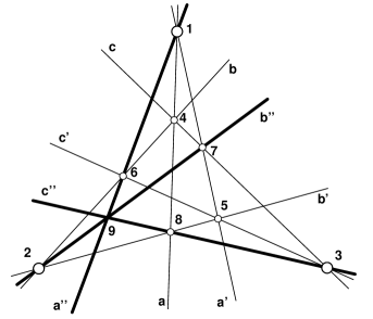
Figure 21. Pappus’ theorem in classical projective geometry. The lines $a^{\prime\prime}$, $b^{\prime\prime}$ and $c^{\prime\prime}$ are drawn in bold.

The following statement expresses one version of Pappus’ Theorem that holds in the usual projective plane over an arbitrary field.

Pappus’ Theorem, incidence version: Let $a,a^{\prime},a^{\prime\prime},b,b^{\prime},b^{\prime\prime},c,c^{\prime},c^{\prime\prime}$ be nine distinct lines in the projective plane. If the following triples of lines

$$[a,a^{\prime},a^{\prime\prime}],[b,b^{\prime},b^{\prime\prime}],[c,c^{\prime},c^{\prime\prime}],[a,b,c],[a^{\prime},b^{\prime},c^{\prime}],[a^{\prime\prime},b,c^{\prime}],[a^{\prime},b^{\prime\prime},c],[a,b^{\prime},c^{\prime\prime}]$$

are concurrent then also $[a^{\prime\prime},b^{\prime\prime},c^{\prime\prime}]$ are concurrent.

In Figure 21, the points in which the lines meet are labeled by $1,\ldots,8$. The final common intersection point of the three lines $a^{\prime\prime},b^{\prime\prime},c^{\prime\prime}$ is labeled by $9$.

Experimentally, it turns out that a tropical analogue of this statement holds for many instances. However, Figure 21 shows a counterexample, which proves that the above version of Pappus’ Theorem does not generally hold in the tropical plane.

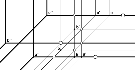
Figure 22. A tropical non-Pappus configuration: the triples $[a,a^{\prime},a^{\prime\prime}]$, $[b,b^{\prime},b^{\prime\prime}]$, $[c,c^{\prime},c^{\prime\prime}]$, $[a,b,c]$, $[a^{\prime},b^{\prime},c^{\prime}]$, $[a^{\prime\prime},b,c^{\prime}]$, $[a^{\prime},b^{\prime\prime},c]$, $[a,b^{\prime},c^{\prime\prime}]$ are concurrent, but $[a^{\prime\prime},b^{\prime\prime},c^{\prime\prime}]$ is not.

In this picture all concurrencies of the hypotheses are satisfied, but the conclusion is violated. Concrete coordinates for the lines in this counterexample are given by the following matrix:

$$\begin{array}{cccccccccc}& a& b& c& a{}^{\prime }& b{}^{\prime }& c{}^{\prime }& a{}^{\prime \prime }& b{}^{\prime \prime }& c{}^{\prime \prime }\\ & -4& -2& -9& -5& -4& -7& 2& 6& 0& \\ & 6& 5& 0& 6& 2& 0& 6& 4& 0& \\ & 0& 0& 0& 0& 0& 0& 0& 0& 0\end{array}$$