Abstract

We consider a Markov chain on the space of (countable) partitions of the interval $[0,1]$, obtained first by size biased sampling twice (allowing repetitions) and then merging the parts (if the sampled parts are distinct) or splitting the part uniformly (if the same part was sampled twice). We prove a conjecture of Vershik stating that the Poisson-Dirichlet law with parameter  $\theta\!=\!1$  is the unique invariant distribution for this Markov chain. Our proof uses a combination of probabilistic, combinatoric, and representation-theoretic arguments.

Key Words: Partitions, coagulation, fragmentation, invariant measures, Poisson-Dirichlet.
AMS 2000 Mathematics Subject Classification. Primary 60K35; secondary 60J27, 60G55.

1 Introduction

Let $\Omega_{1}$ denote the space of (ordered) partitions of $[0,1]$, that is

$$\Omega_{1}:=\left\{p\in[0,1]^{\mbox{${\rm I\!N}$}}:\ p_{1}\geq p_{2}\geq...\geq 0,\ |p|_{1}=1\right\},$$

where $|x|_{1}=\sum_{i}|x_{i}|$ for any finite or countable sequence $(x_{i})$. By size-biased sampling according to a point $p\in\Omega_{1}$ we mean picking the $j$-th part $p_{j}$ with probability $p_{j}$. Our interest in this paper is in the following Markov chain on $\Omega_{1}$, which we call a continuous coagulation-fragmentation process (CCF): size-bias sample (with replacement) two parts from $p$. If the same part was picked twice, split it (uniformly), and reorder the partition. If different parts were picked, merge them, and reorder the partition.

We denote by DCF⁽ⁿ⁾ (discrete coagulation-fragmentation) the Markov chain describing the evolution of the cycle lengths of permutations of $\{1,\ldots,n\}$ under random transpositions. The CCF process appears in a variety of contexts, but of particular relevance to us is its occurrence as a natural limit of DCF⁽ⁿ⁾, when $n$ increases, see [16] for a discussion of this and its link with the space of “virtual permutations”.

For any $n\in\mbox{${\rm I\!N}$}$ denote

$${\mathcal{P}}_{n}:=\{\ell=(\ell_{i})_{i\geq 1}\in\{0,1,\ldots,n\}^{\mbox{${\rm I\!N}$}}\ :\ \ell_{1}\geq\ell_{2}\geq\cdots\geq 0,\ |\ell|_{1}=n\}\ \subset n\Omega_{1}\,.$$

(Elements in ${\mathcal{P}}_{n}$ may be thought of as being of length $n$; the remaining entries are necessarily zero).

A sequence $\ell\in{\mathcal{P}}_{n}$ is uniquely determined by its type $(N_{\ell}(k)\!=\!\sharp\{i:\ell_{i}\!\!=\!\!k\})_{{}_{k=1}}^{{}^{n}}$, with $N_{\ell}\!=\!\sum_{{}_{k=1}}^{{}^{n}}\!\!N_{\ell}(k)$ denoting $\ell$’s total number of parts.

The long-time behaviour of the DCF⁽ⁿ⁾, viewed as an evolution in ${\mathcal{P}}_{n}$, is well understood. In particular, see e.g. [4], it possesses a unique stationary distribution given by the Ewens formula:

$$\pi^{(n)}_{S}(\ell)=\left(\prod_{k=1}^{n}k^{N_{\ell}(k)}N_{\ell}(k)!\right)^{-1}=\left(\prod_{i=1}^{n}\ell_{i}\prod_{k=1}^{n}N_{\ell}(k)!\right)^{-1}\,,\hskip 42.67912pt\ell\in{\mathcal{P}}_{n}\,.$$ (1.1)

It is well known, at least since [11, 13, 18], that the measures $\pi^{(n)}_{S}(n\cdot)$ on $\Omega_{1}$ converge weakly to the Poisson-Dirichlet distribution $\widehat{\mu}_{1}$ with parameter $\theta\!=\!1$ (a precise definition of $\widehat{\mu}_{1}$ is given below in Section 2.1). It has been shown in more than one way (cf. [8, 15, 16]) that $\widehat{\mu}_{1}$ is invariant for the CCF transition. This fact, and hints coming from the theory of virtual permutations, led Vershik (see [16]) to

Conjecture 1.1 (Vershik)

$\widehat{\mu}_{1}$ is the unique invariant distribution for the CCF.

Our goal in this article is to prove Vershik’s conjecture. A naive approach toward the proof would be to use the link with the DCF⁽ⁿ⁾ and the fact that the latter converges to the distribution $\pi^{(n)}_{S}$ exponentially fast. However, the rate of that convergence deteriorates with $n$. To overcome this difficulty, our strategy consists of the following steps:

1. We provide a-priori estimates (Proposition 2.1) showing that every invariant distribution for the CCF leads to a good control on the number of “small parts”.

2. We couple the DCF⁽ⁿ⁾ and the CCF in such a way that whenever they start from initial distributions with such control on the tails, the decoupling time is roughly $\sqrt{n}$ (Theorem 3.1)

3. For initial conditions as above, and for an appropriate class of test functions, we show by using some harmonic analysis on the symmetric group that the DCF⁽ⁿ⁾ achieves near equilibrium before the decoupling time (Theorem 4.1).

These steps are then combined in Theorem 5.1 to yield the proof of Vershik’s conjecture.

Our work began from discussions with Bob Brooks on various models for “random Riemann surfaces”. Brooks and Makover [2], [3] studied Riemann surfaces via a dense set of “Belyi surfaces” associated to three-regular graphs on $n$ vertices with an orientation at each vertex. Their construction gives a complete Riemann surface with finite area $\pi n$ for each graph. Uniformly choosing a random three-regular graph gives a probability distribution on Riemann surfaces, see [7] for an accessible account of this model. Practical choice of a random three-regular graph is not so easy when $n$ is large. Brooks proposed a Markov chain method which involved splitting and joining cycles; investigating properties of his algorithm gave rise to the present paper.

We next review some of the literature on this question. Tsilevich, in [16], proves that $\widehat{\mu}_{1}$ is the only CCF-invariant measure that is also invariant under additional symmetry conditions. Pitman, in [15], proves that $\widehat{\mu}_{1}$ is the only CCF-invariant measure which is also invariant under size-biased sampling. Related results appear in [9]. In another direction, it is shown in [14] that $\widehat{\mu}_{1}$ is the only CCF-invariant measure that is analytic in the sense that for any $k$, the law of an independently size-biased sample (with replacement) possesses an analytic density. Finally, Tsilevich in [17] shows that the law of the CCF, initialized at $p=(1,0,\ldots)$, and stopped at a Binomial($n,1/2$) random time, converges to $\widehat{\mu}_{1}$.

We conclude this introduction by noting that in [14], we have introduced a slightly more general model of split-merge transformations, by allowing either the split or the merge operations to be rejected with a certain probability. An invariant measure for these generalizations is the Poisson-Dirichlet law of parameter $\theta>0$. The discrete counterpart of this chain has been analyzed in [5, Section 4]. While it is plausible that the techniques of the current paper can be adapted to that setup using the results of [5], we do not pursue this generalization here.

2 Continuous and Discrete Coagulation-Fragmentation

2.1 Preliminaries and CCF

Given a topological space $W$, its Borel $\sigma$-algebra will be denoted by ${\mathcal{B}}_{W}$, and the space of probability measures on $(W,{\mathcal{B}}_{W})$ by ${\mathcal{M}}_{1}(W)$. By a slight abuse of notations, ${\mathcal{M}}_{1}(V)$ will also be ${\mathcal{M}}_{1}(W)$’s subspace of probability measures whose support is contained in a given closed subset $V$ of $W$. The total variation of a measure $\nu$ is denoted by $\|\nu\|_{\mbox{\scriptsize var}}$.

We equip $\Omega_{1}$ with its relative $|\cdot|_{{}_{1}}$–topology which, on $\Omega_{1}$, coincides with the weak (coordinatewise convergence) topology.

On $\Omega_{1}$ we consider the Markov chain CCF in which two segments $p_{i}$ and $p_{j}$ of a given partition $p$ are size-bias sampled with replacement and then, if $i\!\neq\!j$ they merge into one of length $p_{i}+p_{j}$ (coagulation), while if $i\!=\!j,\ p_{i}$ splits into two new parts $up_{i},(1-u)p_{i}$ with $u\sim U[0,1]$ independent of all the rest (fragmentation). In either case the new partition is then rearranged nonincreasingly.

Recall that the Poisson-Dirichlet law $\widehat{\mu}_{1}$ is invariant for the CCF transition. Indeed, $\widehat{\mu}_{1}$ itself has been defined in a variety of manners ([1, 11]) which are well known to be equivalent. Perhaps the simplest is the GEM description in which segments are successively and uniformly removed from whatever remains of $[0,1]$, and then rearranged nonincreasingly. Namely, let $Y_{1}\!\!=\!\!1$ and for $n\!\in\!\mbox{${\rm I\!N}$}$ define $X_{n}\!=\!U_{n}\,Y_{n},\$ (the removed part at stage $n$) and $\ Y_{n+1}\!=\!Y_{n}\!-\!X_{n}$ (the remaining segment from which the $(n+1)$-th part is to be removed), where the $U_{n}$’s are independent $U[0,1]$ variables. Since $Y_{n+1}\!=\!(1\!-\!U_{n})Y_{n}$ it follows that $1\!\!-\!\!Y_{n+1}\!=\!\sum_{i=1}^{n}X_{i}$ increases almost surely to $1$ as $n\to\infty$. The distribution on $\Omega_{1}$ of the nonincreasing rearrangement $(p_{i})_{i}$ of $(X_{n})_{n}$ is called the Poisson–Dirichlet law (with parameter $\theta=1$) and denoted $\widehat{\mu}_{1}$.

As has been mentioned in the Introduction, it is the ultimate goal of this work to show that the Poisson-Dirichlet law is the only CCF-invariant probability distribution. It will be crucial for the main argument to establish in advance that any such invariant distribution does not put too much weight on very small parts:

Proposition 2.1

Let $\mu\in{\mathcal{M}}_{1}(\Omega_{1})$ be CCF-invariant. Then

$$\int\sum_{i\geq 1}p_{i}^{\alpha}\ d\mu<\infty\qquad\mbox{for all $\alpha>2/5.$}$$ (2.1)

The proof is deferred to the Appendix.

2.2 DCF

In this section we formally introduce the coagulation–fragmentation chain on the discrete version of $\Omega_{1}$, in which the partition points lie on a finite equidistant grid in $[0,1]$, or its equivalent state space ${\mathcal{P}}_{n}$, the set of integer partitions of a fixed $n\in\mbox{${\rm I\!N}$}$ defined in the Introduction. It will be helpful to view ${\mathcal{P}}_{n}$ as the conjugacy classes of the permutation group $S_{n}$.

The DCF⁽ⁿ⁾ Markov chain on ${\mathcal{P}}_{n}$ is defined similarly to the CCF chain on $\Omega_{1}$. Identify each $\ell\in{\mathcal{P}}_{n}$ with a partition $\bigcup_{i}\!A_{i}$ of $\{1,2,\ldots,n\}$, where for each $i$, $\ell_{i}$ denotes the cardinality of $A_{i}$, and sample two independent integers $x,y$ uniformly from $\{1,\ldots,n\}$ and without replacement, say $x\!\!\in\!\!A_{i}$ and $y\!\!\in\!\!A_{j}$. If $i\neq j$ replace $A_{i}$ and $A_{j}$ by $A_{i}\cup A_{j}$ while if $i=j$ (in which case $\ell_{i}\geq 2$ since $x\neq y\in A_{i}$) replace $A_{i}$ by two of its subsets, consisting respectively of $A_{i}$’s $k$ smallest elements and of the $\ell_{i}\!-\!k$ remaining ones, where $k$ is uniformly sampled from $\{1,\ldots,\ell_{i}\!-\!1\}$ independently of $x$ and $y$. In either case relabel and rearrange the new $A_{i}$’s if necessary.

The transition matrix $K^{(n)}$ of DCF⁽ⁿ⁾ is described as follows: To split into or merge two parts of different sizes $j$ and $k$ ($1\!\leq\!j\!<\!k\!\leq\!n$), let $\ell,\ell^{\prime}\!\in\!{\mathcal{P}}_{n}$ be such that $N_{\ell^{\prime}}(j)\!=\!N_{\ell}(j)\!-\!1,\ \,N_{\ell^{\prime}}(k)\!=\!N_{\ell}(k)\!-\!1,\ N_{\ell^{\prime}}(j\!+\!k)\!=\!N_{\ell}(j\!+\!k)\!+\!1$  and   $N_{\ell^{\prime}}(q)\!=\!N_{\ell}(q)$ for all $q\!\not\in\!\{j,k,j+k\}$. Then

$$K^{(n)}(\ell,\ell^{\prime}) = \frac{2jk}{n(n-1)}\,N_{\ell}(j)N_{\ell}(k)\hskip 41.25641pt\mbox{merge}$$

$$K^{(n)}(\ell^{\prime},\ell) = \frac{2(j+k)}{n(n-1)}\,N_{\ell^{\prime}}(j+k)\hskip 48.36958pt\mbox{split.}$$ (2.2)

To split into or merge two parts of the same size $j$ with $2\leq 2j\leq n$ let $\ell,\ell^{\prime}\in{\mathcal{P}}_{n}$ and $0\leq N_{\ell^{\prime}}(j)=N_{\ell}(j)-2$, $N_{\ell^{\prime}}(2j)=N_{\ell}(2j)+1$, and $N_{\ell^{\prime}}(q)\!=\!N_{\ell}(q)$ for all $q\!\not\in\!\{j,2j\}$. Then

$$K^{(n)}(\ell,\ell^{\prime}) = \frac{j^{2}}{n(n-1)}\,N_{\ell}(j)(N_{\ell}(j)-1)\hskip 41.25641pt\mbox{merge}$$

$$K^{(n)}(\ell^{\prime},\ell) = \frac{2j}{n(n-1)}\,N_{\ell^{\prime}}(2j)\hskip 91.04872pt\mbox{split}$$ (2.3)

All other entries of the transition kernel are zero.

It is customary to think of the representation $\{1,2,\ldots,n\}=\bigcup\!A_{i}$ above as the notation for the conjugacy class of a permutation $\sigma\in S_{n}$. Seen this way, the DCF⁽ⁿ⁾ transition is nothing but the action of a random transposition on $S_{n}$’s conjugacy classes. Since the random transposition’s unique stationary probability measure is the uniform law on $S_{n}$ (being a finite group convolution), one concludes that the DCF⁽ⁿ⁾’s unique stationary probability measure is the one induced on $S_{n}$’s conjugacy classes by the uniform law, namely (1.1) (the Ewens sampling formula). In fact, DCF⁽ⁿ⁾ is reversible with respect to $\pi^{(n)}_{S}$, which can also be checked directly by using (2.2), (2.2) and (1.1) to verify the detailed balance equation $K^{(n)}(\ell,\ell^{\prime})\pi^{(n)}_{S}(\ell)=K^{(n)}(\ell^{\prime},\ell)\pi^{(n)}_{S}(\ell^{\prime})$.

3 Coupling of CCF and DCF

In order to successfully approximate a CCF chain by DCF⁽ⁿ⁾ chains as $n\to\infty$ it is necessary to couple them on a common probability space.

Theorem 3.1

For all $\mu\in{\mathcal{M}}_{1}(\Omega_{1})$ and $\alpha<1/2$ satisfying

$$\int\sum_{i\geq 1}p_{i}^{\alpha}\ d\mu<\infty,$$ (3.1)

it is possible to define for all $n\geq 1$ a CCF Markov chain $p(k)\ (k\geq 0)$ with initial distribution $\mu$ and a $DCF^{(n)}$ Markov chain $\ell(k)\ (k\geq 0)$ on the same probability space with probability measure $Q_{\mu}^{(n)}$ and expectation $E_{\mu}^{(n)}$ in such a way that

$$\lim_{n\to\infty}Q_{\mu}^{(n)}\left[N_{\ell(0)}\geq n^{\beta}\right] = 0\quad\mbox{for all $\alpha<\beta$ and}$$ (3.2)

$$\lim_{n\to\infty}E_{\mu}^{(n)}\left[\left|p(\lfloor n^{\beta}\rfloor)-\frac{\ell(\lfloor n^{\beta}\rfloor)}{n}\right|_{1}\right] = 0\quad\mbox{for all $\beta<1/2$.}$$ (3.3)

Proof:  Fix $n\geq 1$. We shall construct a Markov chain $(c_{k},d_{k},e_{k})\ (k\geq 0)$ on the state space

$$\Omega_{cde}^{(n)} := \big{\{}(c,d,e)\ |\ c:[0,n)\to{\mathbb{Z}}\ \mbox{measurable},\quad{\mathbb{Z}}\backslash c[[0,n)]\ \mbox{infinite,}$$

$$\hskip 51.21495ptd:\{1,\ldots,n\}\to{\mathbb{Z}},\quad e\in\{0,1\}\big{\}}.$$

Here $c$ and $d$ describe a continuous partition of $[0,n)$ and a discrete partition of $\{1,\ldots,n\}$, respectively. The interpretation of $c$ and $d$ in terms of elements of $\Omega_{1}$ and ${\mathcal{P}}_{n}$ is given by the functions $\pi_{c}:\ \Omega_{cde}^{(n)}\to\Omega_{1}$ and $\pi_{d}:\ \Omega_{cde}^{(n)}\to{\mathcal{P}}_{n}$, respectively, defined by

$$\pi_{c}(c,d,e) := {\rm sort\,}\left(\left(\frac{{\rm Leb\,}(c^{-1}(\{i\}))}{n}\right)_{i\in{\mathbb{Z}}}\right)\qquad\mbox{and}$$ (3.4)

$$\pi_{d}(c,d,e) := {\rm sort\,}((\sharp d^{-1}(\{i\}))_{i\in{\mathbb{Z}}}).$$ (3.5)

Here Leb denotes the Lebesgue measure and ${\rm sort\,}((x_{i})_{i})$ is the sequence obtained by arranging the $x_{i}$’s in decreasing order, ignoring the 0’s if there are infinitely many positive $x_{i}$’s. Thus two points $x,y\in[0,n)$ belong to the same set in the partition of $[0,n)$ which is described by $c$ iff $c(x)=c(y)$. Analogously, $x,y\in\{1,\ldots,n\}$ belong to the same set in the partition of $\{1,\ldots,n\}$ described by $d$ iff $d(x)=d(y)$. The CCF Markov chain $p(k)$ and the DCF⁽ⁿ⁾ Markov chain $\ell(k)$ will be realized as

$$p(k):=\pi_{c}(c_{k},d_{k},e_{k})\quad\mbox{and}\quad\ell(k):=\pi_{d}(c_{k},d_{k},e_{k}).$$ (3.6)

The flag $e_{k}$ indicates whether the coupling between the two processes $p(k)$ and $\ell(k)$ is considered to be still in force ($e=0$) or to have already broken down ($e=1$).

The distribution of $(c_{0},d_{0},e_{0})$, that is the initial distribution of the Markov chain, is defined as the image of $\mu$ under the function $\Phi^{(n)}=(\Phi_{1}^{(n)},\Phi_{2}^{(n)},0):\Omega_{1}\longrightarrow\Omega_{cde}^{(n)}$ which assigns to each element of $\Omega_{1}$ an equivalent function $c$ and an approximating function $d$ as follows (see Figure 1):

$$\Phi_{1}^{(n)}(p)(x) := \sum_{j\geq 1}j{\boldsymbol{1}}\left\{x\in[0,np_{j})+n\sum_{i=1}^{j-1}p_{i}\right\}\hskip 31.29802pt(x\in[0,n))$$

$$\Phi_{2}^{(n)}(p)(m) := \Phi_{1}^{(n)}(p)(m-1)\hskip 113.81102pt(m\in\{1,\ldots,n\}).$$

Thus $p(0)=p$ and $\ell(0)=\pi_{d}(\Phi^{(n)}(p))$ are the initial continuous and discrete partitions generated by $p\in\Omega_{1}$.

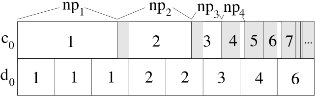
Figure 1: Constructing a continuous partition of $[0,n)$ and a discrete partition of $\{1,\ldots n\}$ from a partition $p\in\Omega_{1}$. Here $n=8$. The shaded area indicates the region where the continuous and the discrete numbering disagree.

Proof of (3.2): To bound $N_{\ell(0)}$, the number of parts in $\ell(0)$, observe that all the pieces in $p$ of size less than $1/n$ can give rise to at most $\sum_{i}np_{i}{\boldsymbol{1}}_{np_{i}<1}$ parts (singletons) in $\ell(0)$. Therefore,

$$N_{\ell(0)} = \#\Phi_{2}^{(n)}(p)[\{1,\ldots,n\}]\ =\ \sum_{i}{\boldsymbol{1}}_{np_{i}\geq 1}+np_{i}{\boldsymbol{1}}_{np_{i}<1}$$ (3.7)

$$\leq \sum_{i}(np_{i})^{\alpha}{\boldsymbol{1}}_{np_{i}\geq 1}+(np_{i})^{\alpha}{\boldsymbol{1}}_{np_{i}<1}\ =\ n^{\alpha}\sum_{i}p_{i}^{\alpha}.$$

Consequently, due to assumption (3.1),

$$E_{\mu}^{(n)}[N_{\ell(0)}]=O(n^{\alpha})$$ (3.8)

and hence, for all $\beta>\alpha$,

$$Q_{\mu}^{(n)}\left[N_{\ell(0)}>n^{\beta}\right]\leq n^{-\beta}E_{\mu}^{(n)}[N_{\ell(0)}]=O(n^{\alpha-\beta}),$$

thus proving (3.2).

We now define informally the kernel of the Markov chain $(c_{k},d_{k},e_{k})$ with state space $\Omega_{cde}^{(n)}$. Assume that the current state of the Markov chain is $(c,d,e)$. To compute the state $(\bar{c},\bar{d},\bar{e})$ the Markov chain is going to jump to in the next step we generate four random variables $\xi_{1},\xi_{2},\zeta_{1}$ and $\zeta_{2}$ such that $\xi_{1}$ and $\xi_{2}$ and $(\zeta_{1},\zeta_{2})$ are independent of each other and of everything else and such that the $\xi_{i}$ are uniformly distributed on $[0,n)$ and $(\zeta_{1},\zeta_{2})$ is uniformly distributed on $[0,n)^{2}\backslash\bigcup_{j=1}^{n}[j-1,j)^{2}$. The $\xi_{i}$ will serve to sample uniformly with replacement from $[0,n)$ whereas the $\zeta_{i}$ will be used to sample uniformly without replacement from $\{1,\ldots,n\}$ in case the $\xi_{i}$ have chosen the same atom in $d$ twice. The new continuous partition $\bar{c}$ is then defined as follows:

$$\mbox{If}\quad c(\xi_{1}) \neq c(\xi_{2}):$$

$$\bar{c}(x) = \left\{\begin{array}[]{ll}c(\xi_{1})&\mbox{if $c(x)=c(\xi_{2})$}\\ c(x)&\mbox{else.}\end{array}\right.$$ (3.11)

$$\mbox{If}\quad c(\xi_{1}) = c(\xi_{2}):$$

$$\bar{c}(x) = \left\{\begin{array}[]{ll}{\rm new\,}(c,d)&\mbox{if $c(x)=c(\xi_{1})$ and $x>\xi_{1}$}\\ c(x)&\mbox{else.}\end{array}\right.$$ (3.14)

We see that the two parts are indeed chosen with probabilities given by their size. In (3.11) two different sets, of sizes ${\rm Leb\,}(c^{-1}(c(\{\xi_{i}\})),\ i=1,2,$ have been selected and are merged by assigning the set $c^{-1}(c(\{\xi_{2}\})$, hit by $\xi_{2}$, the number $c(\{\xi_{1}\})$ of the set $c^{-1}(c(\{\xi_{1}\})$, selected by $\xi_{1}$. This creates a new set $\bar{c}^{-1}(c(\xi_{1}))$ with Lebesgue measure ${\rm Leb\,}(c^{-1}(c(\xi_{1})))+{\rm Leb\,}(c^{-1}(c(\xi_{2})))$.
In (3.14) the set $c^{-1}(c(\{\xi_{1}\})=c^{-1}(c(\{\xi_{2}\})$ is chosen twice, so it has to be split. Since $\xi_{1}$ is conditionally uniformly distributed on this set we can reuse it as splitting point for that set: The part to the left of $\xi_{1}$ retains its old number $c(\xi_{1})=c(\xi_{2})$ whereas the part to its right gets a new number ${\rm new\,}(c,d)$, which is not in the range of $c$ or $d$. Note that it is always possible to find such a new number since ${\mathbb{Z}}\backslash c[[0,n)]$ is assumed to be infinite. By comparing this with the definition of CCF given at the beginning of the Introduction we see that $p(k)$ defined in (3.6) is a CCF Markov chain.

In the discrete case, the two parts chosen are the ones containing the numbers $\lceil\xi_{1}\rceil$ and $\lceil\xi_{2}\rceil$, which ensures that the parts are chosen size biased. The rule for merges in the discrete partition is analogous to (3.11):

$$\mbox{If}\quad d(\lceil\xi_{1}\rceil) \neq d(\lceil\xi_{2}\rceil):$$

$$\bar{d}(m) = \left\{\begin{array}[]{ll}d(\lceil\xi_{1}\rceil)&\mbox{if $d(m)=d(\lceil\xi_{2}\rceil)$}\\ d(m)&\mbox{else.}\end{array}\right.$$ (3.17)

Here two different parts with numbers $d(\lceil\xi_{1}\rceil)$ and $d(\lceil\xi_{2}\rceil)$ have been chosen. They are merged by giving both of them the number $d(\lceil\xi_{1}\rceil)$.
The rule for splitting is slightly more complicated. If the same part (but not the same atom) is sampled twice by the $\xi_{i}$ then again, as in the continuous setting, $\xi_{1}$ determines the point at which the set $d^{-1}(\{\lceil\xi_{1}\rceil\})$ is going to be split: The points to the left of $\lceil\xi_{1}\rceil$ and the points to the right of $\lceil\xi_{1}\rceil$ will constitute the two new fragments. The point $\lceil\xi_{1}\rceil$ itself will be attached to the left or the right part in such a way that the splitting rule for DCF⁽ⁿ⁾, given in (2.2) and (2.2), is imitated. This is done as follows:

$$\mbox{If}\quad d(\lceil\xi_{1}\rceil) = d(\lceil\xi_{2}\rceil)\quad\mbox{and}\quad\lceil\xi_{1}\rceil\neq\lceil\xi_{2}\rceil:$$

$$\bar{d}(m) = \left\{\begin{array}[]{ll}{\rm new\,}(c,d)&\mbox{if $d(m)=d(\lceil\xi_{1}\rceil)$ and $m>\lceil\xi_{1}\rceil$}\\ &\mbox{or}\ m=\lceil\xi_{1}\rceil\ \mbox{and}\ \xi_{1}<\lfloor\xi_{1}\rfloor+{\displaystyle\frac{\#d^{-1}(\{d(\lceil\xi_{1}\rceil)\})\cap[0,\xi_{1}]}{\#d^{-1}(\{d(\lceil\xi_{1}\rceil)\})-1}}\\ d(m)&\mbox{else}.\\ \end{array}\right.$$ (3.21)

Indeed, consider for simplicity the case that the atoms of the set $d^{-1}(\{d(\lceil\xi_{1}\rceil)\})$ are not scattered around the whole set $\{1,\ldots,n\}$, which they typically will be, but are collected at the bottom: $d^{-1}(\{d(\lceil\xi_{1}\rceil)\})=\{1,\ldots,a\}$, where $a:=\sharp d^{-1}(\{d(\lceil\xi_{1}\rceil)\})$. Definition (3.21) tells us that this set is split into $\{1,\ldots,j\}$ and $\{j+1,\ldots,a\}$ if

$$j-1+\frac{j-1}{a-1}\leq\xi_{1}<j+\frac{j}{a-1}.$$

Conditioned on $\xi_{1}\in[0,a)$, the probability for this to happen is $1/(a-1)$. This means that the discrete set $\{1,\ldots,a\}$ is indeed split as described at the beginning of Section 2.2.

If however the same atom in $d$ has been sampled twice by the $\xi_{i}$’s, i.e. $\lceil\xi_{1}\rceil=\lceil\xi_{2}\rceil$, then $\xi_{1}$ and $\xi_{2}$ are disregarded and $\bar{d}(n)$ is defined as in (3.17) and (3.21) but with $(\xi_{1},\xi_{2})$ replaced by $(\zeta_{1},\zeta_{2})$ in order to sample without replacement. The process $\ell(k)$ defined in (3.6) is a DCF⁽ⁿ⁾ Markov chain.

It remains to define $\bar{e}$:

$$\bar{e}=\left\{\begin{array}[]{ll}1&\mbox{if $\lceil\xi_{1}\rceil=\lceil\xi_{2}\rceil$ or $c(\xi_{1})\neq d(\xi_{1})$ or $c(\xi_{2})\neq d(\xi_{2})$}\\ e&\mbox{else.}\end{array}\right.$$

In the case $\bar{e}=1$ the coupling has broken down: Either the same atom in the discrete partition has been sampled twice by the $\xi_{i}$’s or at least one of the $\xi_{i}$’s belongs to non-corresponding sets in the continuous and the discrete partition. The time $\tau:=\inf\{k\geq 1:\ e_{k}=1\}$ is regarded as the decoupling time of the chains $p(k)$ and $\ell(k)$.
The definition of the transition kernel for the Markov chain on $\Omega_{cde}^{(n)}$ is now complete. It is summarized in Figures 2 to 4.

Figure 2: Merging the parts with numbers 1 and 2.

Figure 3: Splitting the part with number 4 into a part with number 4 and a part with number ${\rm new}\,(c,d)=0$.

Figure 4: Two ways to decouple the chains: Sampling from the region where $c$ and $d$ disagree ($\xi_{2}$, top) or sampling with replacement from $d$ ($\xi_{1}$ and $\xi_{2}$, bottom).

Proof of (3.3): We denote by

$$\varrho_{k}:={\rm Leb\,}(\{x\in[0,n)\ :\ c_{k}(x)\neq d_{k}(\lceil x\rceil\}).$$

the discrepancy between $c_{k}$ and $d_{k}$. For $k=0$, this is the roundoff error caused by the approximation of $c_{0}$ by $d_{0}$; its size is the length of the shaded area in Figure 1. Note that

$$\varrho_{0}\leq N_{\ell(0)}$$ (3.22)

because any part in $d_{0}$ might disagree with $c_{0}$ at most in its right most atom. Moreover, $\varrho_{k}$ can increase in each step by at most 1 as long as $k<\tau$: Indeed, if two parts are merged, $\varrho_{k}$ does not increase at all (it might even decrease) whereas it might increase by at most ${\rm Leb\,}((\lfloor\xi_{1}\rfloor,\lceil\xi_{1}\rceil])=1$ in case of splitting. Hence, $\varrho_{k+1}\leq\varrho_{k}+1$ if $k<\tau$ and therefore,

$$\varrho_{k}\leq\varrho_{0}+k\quad\mbox{on the event}\quad\{k<\tau\}.$$ (3.23)

Since the $|\cdot|_{1}$-diameter of $\Omega_{1}$ is at most 2 we have

$$E_{\mu}^{(n)}\left[\left|p(\lfloor n^{\beta}\rfloor)-\frac{\ell(\lfloor n^{\beta}\rfloor)}{n}\right|_{1}\right]$$ (3.24)

$$\leq E_{\mu}^{(n)}\left[\left|p(\lfloor n^{\beta}\rfloor)-\frac{\ell(\lfloor n^{\beta}\rfloor)}{n}\right|_{1},\lfloor n^{\beta}\rfloor\leq\tau\right]+2Q_{\mu}^{(n)}[\tau<\lfloor n^{\beta}\rfloor].$$

We are going to bound the first term in (3.24) first. It is easy to see that $|p-q|_{1}\geq|{\rm sort\,}(p)-{\rm sort\,}(q)|_{1}$ for any two summable sequences $p=(p_{i})_{i}$ and $q=(q_{i})_{i}$ of non-negative numbers. Indeed, if $p_{i}>p_{j}$ and $q_{i}<q_{j}$, then swapping $q_{i}$ and $q_{j}$ would not increase $|p-q|_{1}$. Therefore, by definitions (3.4), (3.5) and (3.6) on the event $\{\lfloor n^{\beta}\rfloor<\tau\}$,

$$\left|p(\lfloor n^{\beta}\rfloor)-\frac{\ell(\lfloor n^{\beta}\rfloor)}{n}\right|_{1} \leq \frac{1}{n}\sum_{i\geq 1}\left|{\rm Leb\,}(c_{\lfloor n^{\beta}\rfloor}^{-1}(\{i\}))-\#d_{\lfloor n^{\beta}\rfloor}^{-1}(\{i\})\right|$$

$$\leq \frac{1}{n}\sum_{i\geq 1}{\rm Leb\,}(\{x:i\in\{c_{\lfloor n^{\beta}\rfloor}(x),d_{\lfloor n^{\beta}\rfloor}(x)\},c_{\lfloor n^{\beta}\rfloor}(x)\neq d_{\lfloor n^{\beta}\rfloor}(x)\})$$

$$\leq \frac{2}{n}\varrho_{\lfloor n^{\beta}\rfloor}\ \leq\ \frac{2}{n}(\varrho_{0}+\lfloor n^{\beta}\rfloor)\ \leq\ \frac{2}{n}(N_{\ell(0)}+\lfloor n^{\beta}\rfloor)$$

by (3.23) and (3.22). Consequently, due to (3.8), the first term in (3.24) is of order $O(n^{\alpha-1}+n^{\beta-1})$, thus going to 0 as $n\to\infty$.

To show that the second term in (3.24) goes to 0 as well we assume without loss of generality that $\alpha<\beta<1/2$. Consider the probability that a chain which has not decoupled until the $k$th step will decouple in the $(k+1)$th step. Given $\varrho_{0},\ldots,\varrho_{k}$, the event that $\xi_{1}$ samples two different parts in $c_{k}$ and $d_{k}$ has probability $\varrho_{k}/n$. The same holds for $\xi_{2}$. Moreover, the event that one atom in $d_{k}$ is sampled twice, i.e. that $\lceil\xi_{1}\rceil=\lceil\xi_{2}\rceil$ has probability $1/n$. Therefore, the probability that either of these events occurs and the chain decouples is at most $(2\varrho_{k}+1)/n$. On the event $\{\tau>k,\varrho_{0}<n^{\beta}\}$ this can be bounded from above due to (3.23) by $(2(n^{\beta}+k)+1)/n$ which is less than $5n^{\beta-1}$ if $k\leq n^{\beta}$. Thus we get by induction over $k$,

$$Q_{\mu}^{(n)}[\tau>k,\varrho_{0}<n^{\beta}]\geq(1-5n^{\beta-1})^{k}Q_{\mu}^{(n)}[\varrho_{0}<n^{\beta}]$$

for all $k\leq n^{\beta}$ and hence

$$Q_{\mu}^{(n)}[\tau\geq\lfloor n^{\beta}\rfloor] \geq \left(\left(1-5n^{\beta-1}\right)^{n^{1-\beta}}\right)^{n^{2\beta-1}}Q_{\mu}^{(n)}\left[\varrho_{0}<n^{\beta}\right].$$ (3.25)

Due to $2\beta-1<0$, the first factor in (3.25) converges to one as $n\to\infty$. The same holds for the second factor due to (3.22) and (3.2). Consequently, also the second term in (3.24) goes to 0, which completes the proof of (3.3).      

4 DCF⁽ⁿ⁾ convergence

It was mentioned in the Introduction, that the uniform rate of convergence to $\pi^{(n)}_{S}$ is too weak to combine properly with $n\to\infty$. However, according to the following theorem (to be proved in subsection 4.2), the situation is better when starting off from partitions with relatively few parts and restricting our attention to a certain family $\mathcal{C}$ of $\Omega_{1}$–neighborhoods to be defined below. For every $n\in\mbox{${\rm I\!N}$}$ and $\beta\in(0,1]$, thus, denote accordingly

$${\mathcal{P}}_{n,\beta} = \left\{\ell\in{\mathcal{P}}_{n}\,:\ N_{\ell}<n^{\beta}\right\}=\left\{\ell\in{\mathcal{P}}_{n}\,:\ \ell_{\lceil n^{\beta}\rceil}=0\ \right\}\ .$$

As for the definition of $\mathcal{C}$, for each $k\!\in\!\mbox{${\rm I\!N}$}$ let

$$I_{k}=\left\{(\mbox{\boldmath$a$},\mbox{\boldmath$b$})\!=\!(a_{i},b_{i})_{i=1}^{k}\,:\ \ \ 0<a_{i}<b_{i}<1\,\ \ \ \sum_{i=1}^{k}b_{i}\!<\!1,\ \ \ \ \ a_{k}\!>\!1\!-\!\sum_{i=1}^{k}a_{i}\ \right\}$$ (4.1)

and denote $\delta_{\mbox{\boldmath\scriptsize{$a$}},\mbox{\boldmath\scriptsize{$b$}}}\!=\!\min\left\{1\!-\!\sum_{i=1}^{k}b_{i}\ \ ,\ \ a_{k}\!-\!(1\!-\!\sum_{i=1}^{k}a_{i})\right\}$. Then, for each $(\mbox{\boldmath$a$},\mbox{\boldmath$b$})\in I_{k}$, define

$$C_{\mbox{\boldmath\scriptsize{$a$}},\mbox{\boldmath\scriptsize{$b$}}}=\left\{x\in\Omega_{1}\,:\ x_{i}\in(a_{i},b_{i})\ \ \ \mbox{for}\ i=1,\ldots,k\right\}\hskip 142.26378pt$$ (4.2)

which is nonempty if and only if   $0\!<\!a_{i}\!\!<\!\!\underset{1\leq j\leq i}{\min}b_{j}$   for $i=1,\ldots,k$,   in which case the conditions on $(\mbox{\boldmath$a$},\mbox{\boldmath$b$})\!\in\!I_{k}$ guarantee that

$$C_{\mbox{\boldmath\scriptsize{$a$}},\mbox{\boldmath\scriptsize{$b$}}}\!=\!\left\{x=(x^{\prime},x^{\prime\prime})\ :\ x^{\prime}\in G_{{\mbox{\boldmath\scriptsize{$a$}},\mbox{\boldmath\scriptsize{$b$}}}},\ x^{\prime\prime}\in(1-|x^{\prime}|_{1})\Omega_{1}\right\}.\hskip 113.81102pt$$ (4.3)

(Here $(\,\cdot\,,\,\cdot\,)$ denotes concatenation and $G_{\mbox{\boldmath\scriptsize{$a$}},\mbox{\boldmath\scriptsize{$b$}}}$ is the (nonempty) subset of points in $\prod_{{}_{i=1}}^{{}^{k}}\!(a_{i},b_{i})$ whose coordinates are nonincreasing). Moreover, $I_{k}$’s definition (4.1) implies that

$$\delta_{\mbox{\boldmath\scriptsize{$a$}},\mbox{\boldmath\scriptsize{$b$}}}<|x^{\prime\prime}|_{1}<x^{\prime}_{k}-\delta_{\mbox{\boldmath\scriptsize{$a$}},\mbox{\boldmath\scriptsize{$b$}}}\ ,\hskip 42.67912pt\forall(x^{\prime},x^{\prime\prime})\in C_{\mbox{\boldmath\scriptsize{$a$}},\mbox{\boldmath\scriptsize{$b$}}}\ .\hskip 128.0374pt$$ (4.4)

Finally,

$$\mathcal{C}=\{C_{\mbox{\boldmath\scriptsize{$a$}},\mbox{\boldmath\scriptsize{$b$}}}\,:\,(\mbox{\boldmath$a$},\mbox{\boldmath$b$})\in I_{k},\ k\geq 1\}.$$ (4.5)

The family $\mathcal{C}$ of $\Omega_{1}$–neighborhoods will be shown in Section 5 to be sufficiently rich to characterize $\widehat{\mu}_{1}$ uniquely. At the same time, and as a result of their special features (4.3) and (4.4), the convergence of the DCF⁽ⁿ⁾ to its equilibrium is fast on the sets in $\mathcal{C}$:

Theorem 4.1

Fix $\beta\!\in\!(0,\frac{1}{2})$. For each $n\!\in\!\mbox{${\rm I\!N}$}$ let $\left(X^{(n)}(k)\right)_{k\geq 0}$ be a DCF⁽ⁿ⁾ Markov chain with underlying probability measure $P^{(n)}$ and initial distribution $\mu_{0}^{(n)}\!\in\!{\mathcal{M}}_{1}({\mathcal{P}}_{n,\beta})$. Then for any $C\!\in\!\mathcal{C}$, $\beta^{\prime}\!>\!\beta$ and integer sequence $k=k_{n}\geq n^{\beta^{\prime}}$

$$\Delta_{C}^{(n)}(k):=P^{(n)}\left(X^{(n)}(k)\in nC\right)-\pi^{(n)}_{S}(nC)\underset{n\to\infty}{\longrightarrow}0\,.$$

4.1 Characters in $S_{n}$ – Background

Recall that the partition space ${\mathcal{P}}_{n}$ can be viewed as the quotient of the permutation group $S_{n}$ under conjugacy. Thus the natural inner product on $F_{n}\!:=\!\{f:{\mathcal{P}}_{n}\longrightarrow{{\mathbb{R}}}\}$ is

$$\langle f,g\rangle=\langle f,g\rangle_{{}_{n}}=\sum_{\gamma\in{\mathcal{P}}_{n}}f(\gamma)g(\gamma)\pi^{(n)}_{S}(\gamma)\ .$$

The fact mentioned earlier that $\pi^{(n)}_{S}$ is a reversing measure for the DCF⁽ⁿ⁾ means precisely that $K^{(n)}$ is selfadjoint with respect to this inner product.

The following basic facts regarding the character theory of $S_{n}$, as well as the full theory, can be found, for example, in [10], and their relevance to random group actions (such as transpositions in our case) in [4] and  [6]. The characters $\{\chi\}$ of $S_{n}$ (traces of the irreducible representations) are functions on $S_{n}$, constant on conjugacy classes, and as such can be seen to be functions on ${\mathcal{P}}_{n}$. They are orthonormal under $\langle\,\cdot\,,\,\cdot\,\rangle$ and since there are $\#{\mathcal{P}}_{n}$ of them, they are indexed by the partitions ( $(\chi_{{}_{\lambda}})_{{}_{\lambda\in{\mathcal{P}}_{n}}}$) and form an orthonormal base of $F_{n}$.

Since $K^{(n)}$ represents a random transposition, its dual $K^{(n)^{*}}$ acts on ${\mathcal{M}}_{1}(S_{n})$ as a convolution

$$K^{(n)^{*}}\mu=\kappa^{(n)}\star\mu\hskip 56.9055pt\left(\kappa^{(n)}(\mbox{\small{transposition}})\!=\!\frac{2}{n(n\!-\!1)}\ \ \ \mbox{and}\ \ 0\ \ \mbox{otherwise}\right)$$

as a result of which, and of a corollary ([4, Ch. 2, Prop. 6]) of Schur’s lemma,

• $K^{(n)}$’s eigenfunctions are the characters $(\chi_{{}_{\lambda}})_{\lambda\in{\mathcal{P}}_{n}}$

• the eigenvalue $\theta_{\lambda}^{(n)}$ corresponding to $\chi_{{}_{\lambda}}$is given by $\frac{\mbox{\large{$\chi_{{}_{\lambda}}$}}(\mbox{\small{transposition}})}{\mbox{\large{$\chi_{{}_{\lambda}}$}}(\mbox{\small{identity}})}$ .

A result of Frobenius in principle provides formulae for all characters. Although in general they can be intractable, this is not so at transpositions and at the identity, thus yielding ([4, D-2,p.40])

$$\theta_{\lambda}^{(n)}=\frac{1}{n(n-1)}\sum_{j}\lambda_{j}(\lambda_{j}-2j+1)=\frac{1}{n(n-1)}\left(\sum_{i=1}^{n}\lambda_{i}^{2}-\sum_{j=1}^{\lambda_{1}}{\lambda_{j}^{\prime}}^{2}\right)\,.$$ (4.6)

($\lambda$’s adjoint partition $\lambda^{\prime}$ is defined below). In particular $\theta^{(n)}_{(n,0,\ldots)}=1$ and $\chi_{{}_{(n,0,\ldots)}}\equiv 1$.

For many purposes, a partition $\lambda\in{\mathcal{P}}_{n}$ can be best described by its Young diagram $\Upsilon_{{}_{\!\lambda}}$ (Fig. 5), consisting of $N_{\lambda}$ rows of $\lambda_{1},\ldots,\lambda_{N_{\lambda}}$ cells respectively, in terms of which some useful features of $\lambda$ can be defined. The $j$-th cell in row $i$ is denoted $(i,j)$.

• $\lambda^{\prime}\in{\mathcal{P}}_{n}$ is the partition whose Young diagram is obtained from $\lambda$’s by transposition; $\Upsilon_{{}_{\!\lambda^{\prime}}}=\Upsilon_{{}_{\!\lambda}}^{{}^{\mbox{\tiny$T$}}}$

• $B_{\lambda}=\max\{i:(i,i)\in\Upsilon_{{}_{\!\lambda}}\}=\max\{i:\lambda_{i}\geq i\}$          ($\lambda$’s diagonal length)

• $R_{\lambda}(i,j)=\{(u,v)\,:\,\ i\!\leq\!u\!\leq\!\lambda_{j}^{\prime},\ \ j\,\mbox{\footnotesize{$\vee$}}\,\lambda_{u+1}\!\leq\!v\!\leq\!\lambda_{u}\}$          ($\Upsilon_{{}_{\!\lambda}}$’s rim segment straddled by $(i,j)$)

• $\Upsilon_{\!\lambda_{*}^{(i,j)}}=\Upsilon_{{}_{\!\lambda}}\setminus R_{\lambda}(i,j)$ defines $\lambda_{*}^{(i,j)}$     ( a diagram obtained from $\lambda$’s by removing a rim segment is a Young diagram; this defines the partition $\lambda_{*}^{(i,j)}$)

In addition, for any $\gamma\in{\mathcal{P}}_{n}$, define $\gamma^{\widehat{r}}=(\gamma_{1},\ldots,\widehat{\gamma_{r}},\ldots)\in{\mathcal{P}}_{n-\gamma_{r}}$, the partition obtained from $\gamma$ by removing its $r$-th part. The following Murnaghan–Nakayama rule (see [6, Theorem 3.4]) provides a way of recursively evaluating characters: for all $\lambda,\gamma\in{\mathcal{P}}_{n}$  and $1\!\leq\!r\!\leq\!N_{\gamma}$

$$\chi_{{}_{\lambda}}(\gamma)=\sum_{(i,j)\,:\,\#R_{\lambda}(i,j)=\gamma_{r}}(-1)^{\lambda^{\prime}_{j}-i}\,\chi_{{}_{{}_{\!\lambda_{*}^{(i,j)}}}}\!(\gamma^{\widehat{r}})\hskip 142.26378pt$$ (4.7)

in the sense that the sum is zero if its index set is empty, and $\chi_{{}_{\emptyset}}(\mbox{\footnotesize{$\emptyset$}})=1$. Thus, for a fixed order in which $\gamma$’s parts are chosen, $\chi_{{}_{\lambda}}(\gamma)$ can be calculated by covering all possible ways of successively stripping off $\gamma_{r}$–sized rim segments from $\lambda$’s diagram, and $\chi_{{}_{\lambda}}(\gamma)=0$ if it is impossible to exhaust $\Upsilon_{{}_{\!\lambda}}$ entirely in this way. In particular

$$N_{\gamma}<B_{\lambda}\Longrightarrow\chi_{{}_{\lambda}}(\gamma)=0\hskip 199.16928pt$$ (4.8)

since any rim segment of $\lambda$ contains at most one diagonal cell $(i,i)$.

Figure 5: Young diagrams of $\lambda,\gamma\in{\mathcal{P}}_{33}$. Two $\lambda$-cells, $(1,4)$ and $(2,3)$, generate rim segments of size $9$, the latter shown explicitly, which the Murnaghan–Nakayama rule “peels off” together with the deletion of $\gamma_{2}$.

4.2 Proof of Theorem 4.1

Before proceeding with the proof itself, it will be helpful to characterize the $\gamma\in{\mathcal{P}}_{n}$ which belong to $nC\!=\!nC_{\mbox{\boldmath\scriptsize{$a$}},\mbox{\boldmath\scriptsize{$b$}}}$ for given $k\!\in\!\mbox{${\rm I\!N}$}$ and $(\mbox{\boldmath$a$},\mbox{\boldmath$b$})\!\in\!I_{k}$ (assuming $C\mbox{\small{$\neq\emptyset$}}$). It follows from $C_{\mbox{\boldmath\scriptsize{$a$}},\mbox{\boldmath\scriptsize{$b$}}}$’s description (4.3) that any such $\gamma$ can be expressed as a concatenation $(\gamma^{\prime},\gamma^{\prime\prime})$ where $\gamma^{\prime}\!\in\!G^{(n)}_{\mbox{\boldmath\scriptsize{$a$}},\mbox{\boldmath\scriptsize{$b$}}}$ and $\gamma^{\prime\prime}\!\in\!{\mathcal{P}}_{n-|\gamma^{\prime}|_{1}}$, and where $G^{(n)}_{\mbox{\boldmath\scriptsize{$a$}},\mbox{\boldmath\scriptsize{$b$}}}$ consists of nonincreasing integer valued $k$-sequences $\gamma^{\prime}$ which by virtue of (4.4) satisfy

$$\mbox{\bf i)}\ |\gamma^{\prime}|_{1}<n\hskip 42.67912pt\mbox{\bf ii)}\ \exists\delta\!=\!\delta(C)\!>\!0\ \ \mbox{such that}\ \ \gamma^{\prime}_{k}>(n\!-\!|\gamma^{\prime}|_{1})+\delta n\ .$$ (4.9)

This state of affairs is illustrated in Figure 6.

Proof of Theorem 4.1

Fix $C\in\mathcal{C}$ and define $f_{n}={\boldsymbol{1}}_{nC}$. Then, in terms of $\mu_{0}^{(n)}$’s density $g_{0}^{(n)}(\gamma)=\frac{\mu_{0}^{(n)}(\gamma)}{\pi^{(n)}_{S}(\gamma)}$:

$$P^{(n)}\left(X^{(n)}(k)\!\in\!nC\right)\!\! = \!\!\sum_{\gamma}\mu_{0}^{(n)}(\gamma)K^{(n)^{k}}f_{n}(\gamma)=\langle g_{0}^{(n)},K^{(n)^{k}}f_{n}\rangle=\sum_{\lambda\in{\mathcal{P}}_{n}}\!\!\theta_{\lambda}^{(n)^{k}}\langle g_{0}^{(n)},\chi_{{}_{\lambda}}\rangle\langle f_{n},\chi_{{}_{\lambda}}\rangle$$

$$\mbox{and,\ \ since}\ \theta^{(n)}_{(n,0,\ldots)}=1 \chi_{(n,0,\ldots)}\equiv 1,$$ and

$$\pi^{(n)}_{S}(nC) = \langle f_{n},1\rangle=\theta_{(n,0,\ldots)}^{(n)^{k}}\langle g_{0}^{(n)},\chi_{{}_{(n,0,\ldots)}}\rangle\langle f_{n},\chi_{{}_{(n,0,\ldots)}}\rangle$$

so that

$$\Delta_{C}^{(n)}(k)=\sum_{(n,0,\ldots)\neq\lambda\in{\mathcal{P}}_{n}}\theta_{\lambda}^{(n)^{k}}\langle g_{0}^{(n)},\chi_{{}_{\lambda}}\rangle\langle f_{n},\chi_{{}_{\lambda}}\rangle\ .\hskip 116.65646pt$$ (4.10)

By assumption, $g_{0}^{(n)}(\gamma)=0$ whenever $N_{\gamma}>n^{\beta}$. On the other hand, $\chi_{{}_{\lambda}}(\gamma)=0$ whenever $B_{\lambda}>n^{\beta}$ and $N_{\gamma}\leq n^{\beta}$ by the consequence (4.8) of Murnaghan–Nakayama’s rule. Thus (4.10) becomes

$$\Delta_{C}^{(n)}(k)=\!\!\sum_{\underset{B_{\lambda}\leq n^{\beta}}{(n,0,\ldots)\neq\lambda\in{\mathcal{P}}_{n}}}\!\!\theta_{\lambda}^{(n)^{k}}\langle g_{0}^{(n)},\chi_{{}_{\lambda}}\rangle\langle f_{n},\chi_{{}_{\lambda}}\rangle\ .$$

Figure 6: A partition $\gamma$ in $nC_{\mbox{\boldmath\scriptsize{$a$}},\mbox{\boldmath\scriptsize{$b$}}}$ splits into its first $k$ rows $\gamma^{\prime}$ and the remainder $\gamma^{\prime\prime}$ which is nonempty but smaller in size than $\gamma^{\prime}$’s last row.

Now choose an $\eta$ such that $1\!-\!(\beta^{\prime}\!\!-\!\!\beta)<\eta<1$ and let $n_{0}=5^{\frac{1}{1-\eta}}$. Then, for all $n\!\geq\!n_{0}$,

$$\Delta_{C}^{(n)}(k)=\left(\sum_{\lambda\in{\mathcal{P}}_{n}^{\prime}}+\sum_{\lambda\in{\mathcal{P}}_{n}^{\prime\prime}}+\sum_{\lambda\in{\mathcal{P}}_{n}^{\prime\prime\prime}}\right)\theta_{\lambda}^{(n)^{k}}\langle g_{0}^{(n)},\chi_{{}_{\lambda}}\rangle\langle f_{n},\chi_{{}_{\lambda}}\rangle$$ (4.11)

where

$${\mathcal{P}}_{n}^{\prime}={\mathcal{P}}_{n}^{\prime}(\eta,\beta) = \left\{\lambda\in{\mathcal{P}}_{n}:\ \ B_{\lambda}\leq n^{\beta},\ \ \ \lambda_{1}\!\leq\!n\!-\!2n^{\eta},\ \ \ N_{\lambda}\!\leq\!n\!-\!2n^{\eta}\,\right\}$$

$${\mathcal{P}}_{n}^{\prime\prime}={\mathcal{P}}_{n}^{\prime\prime}(\eta,\beta) = \left\{\lambda\in{\mathcal{P}}_{n}:\ \ B_{\lambda}\leq n^{\beta},\ \ \ n\!-\!2n^{\eta}\!<\!\lambda_{1}\!<\!n\,\right\}$$

$${\mathcal{P}}_{n}^{\prime\prime\prime}={\mathcal{P}}_{n}^{\prime\prime\prime}(\eta,\beta) = \left\{\lambda\in{\mathcal{P}}_{n}:\ \ B_{\lambda}\leq n^{\beta},\ \ \ n\!-\!2n^{\eta}\!<\!N_{\lambda}\,\right\}$$

(Our choice of $n_{0}$ ensures that ${\mathcal{P}}_{n}^{\prime\prime}$ and ${\mathcal{P}}_{n}^{\prime\prime\prime}$ are disjoint and that $(n,0,\ldots)\not\in{\mathcal{P}}_{n}^{\prime\prime\prime}$). It turns out that for $n$ large enough, the terms in (4.11) vanish for all $\lambda\in{\mathcal{P}}_{n}^{\prime\prime}\cup{\mathcal{P}}_{n}^{\prime\prime\prime}$, whereas when $\lambda\in{\mathcal{P}}_{n}^{\prime}$ the factor  $|\theta_{\lambda}^{(n)}|$  is sufficiently separated from $1$ :

Lemma 4.2

$\exists n_{1}=n_{1}(\beta,C)$ such that  $\langle f_{n},\chi_{{}_{\lambda}}\rangle=0,\ \ \ \ \forall n\!\geq\!n_{1},\ \forall\lambda\!\in\!{\mathcal{P}}_{n}^{\prime\prime}\cup{\mathcal{P}}_{n}^{\prime\prime\prime}$ .

Lemma 4.3

For all $\lambda\!\in\!{\mathcal{P}}_{n}$,  $|\theta_{\lambda}^{(n)}|\leq\frac{\mbox{\large{$\lambda_{1}\mbox{\footnotesize{$\vee$}}N_{\lambda}$}}}{\mbox{\large{$n$}}}$   and thus   $\exists n_{2}=n_{2}(\eta)$ such that

$$|\theta_{\lambda}^{(n)}|\leq e^{-n^{\eta-1}}\hskip 42.67912pt\forall n\!\geq\!n_{2},\ \ \forall\lambda\!\in\!{\mathcal{P}}_{n}^{\prime}\ .$$ (4.12)

Proof of Lemma 4.2

Consider first $\lambda\!\in\!{\mathcal{P}}_{n}^{\prime\prime}$. Now, $C\!=\!C_{\mbox{\boldmath\scriptsize{$a$}},\mbox{\boldmath\scriptsize{$b$}}}$ for some $k\!\in\!\mbox{${\rm I\!N}$}$ and $(\mbox{\boldmath$a$},\mbox{\boldmath$b$})\!\in\!I_{k}$, so that, as discussed at the beginning of the section and illustrated in Figure 6, $\gamma$ can be split into $(\gamma^{\prime},\gamma^{\prime\prime})$ and

$$\langle f_{n},\chi_{{}_{\lambda}}\rangle=\sum_{\gamma^{\prime}\in G^{(n)}_{\mbox{\boldmath\scriptsize{$a$}},\mbox{\boldmath\scriptsize{$b$}}}}\,\sum_{\ \gamma^{\prime\prime}\in{\mathcal{P}}_{n-|\gamma^{\prime}|_{1}}}\!\!\!\pi^{(n)}_{S}(\gamma^{\prime},\gamma^{\prime\prime})\chi_{{}_{\lambda}}(\gamma^{\prime},\gamma^{\prime\prime})\ .$$ (4.13)

(Note that property (4.9i) guarantees that the inner sum is not vacuous, i.e. $|\gamma^{\prime\prime}|_{1}>0$).

We shall show that for every fixed $\gamma^{\prime}\!\in\!G^{(n)}_{\mbox{\boldmath\scriptsize{$a$}},\mbox{\boldmath\scriptsize{$b$}}}$ the inner sum in (4.13) equals zero. First apply Murnaghan–Nakayama’s rule (4.7) $k$ times to $\chi_{{}_{\lambda}}(\gamma^{\prime},\gamma^{\prime\prime})$ by successively stripping rim segments from $\lambda$, of lengths $\gamma^{\prime}_{i}$ at each stage $i,\ i=1,\ldots,k$. On the one hand $\lambda_{1}\!>\!(1\!-\!\delta)n$ for $n\geq n_{1}^{\prime\prime}=n_{1}^{\prime\prime}(\beta,\eta,C)$ (since $\lambda\!\in\!{\mathcal{P}}_{n}^{\prime\prime}$), and on the other $\gamma^{\prime}_{i}>\delta n,\ i=1,\ldots,k$ (by (4.9ii)). This implies that at each of these $k$ reduction stages precisely one rim segment can be stripped off, namely the last $\gamma^{\prime}_{i}$ cells of whatever remains of $\lambda_{1},i=1,\ldots,k$. Summing up

$$\chi_{{}_{\lambda}}(\gamma^{\prime},\gamma^{\prime\prime})=\chi_{{}_{\lambda^{*}}}(\gamma^{\prime\prime})$$ (4.14)

where $\lambda^{*}\in{\mathcal{P}}_{n-|\gamma^{\prime}|_{1}}$ is defined by $\lambda^{*}_{1}\!=\!\lambda_{1}\!-\!|\gamma^{\prime}|_{1}$ and $\lambda^{*}_{j}\!=\!\lambda_{j},\ j\geq 2$. As for the first factor of the summand in (4.13), note that (4.9ii) implies $\gamma^{\prime}_{k}>\gamma^{\prime\prime}_{1}$ (see Figure 6) and thus

$$\frac{\pi^{(n)}_{S}(\gamma^{\prime},\gamma^{\prime\prime})}{\pi_{S}^{(n-|\gamma^{\prime}|_{1})}(\gamma^{\prime\prime})}=\frac{1}{\prod_{i=1}^{k}\gamma^{\prime}_{i}\prod_{j}N_{\gamma^{\prime}}(j)!}=:R(\gamma^{\prime}).$$ (4.15)

Inserting (4.14) and (4.15) in the inner sum of (4.13) we obtain

$$\sum_{\gamma^{\prime\prime}\in{\mathcal{P}}_{n-|\gamma^{\prime}|_{1}}}\pi^{(n)}_{S}(\gamma^{\prime},\gamma^{\prime\prime})\chi_{{}_{\lambda}}(\gamma^{\prime},\gamma^{\prime\prime})=R(\gamma^{\prime})\langle\chi_{{}_{\lambda^{*}}},1\rangle_{{}_{n-|\gamma^{\prime}|_{1}}}=0$$

since $\lambda^{*}$ is not the trivial partition, that is $\lambda^{*}\neq(n-|\gamma^{\prime}|_{1},0,\ldots)$, (because $\lambda\neq(n,0,\ldots)$), and thus $\chi_{{}_{\lambda^{*}}}$ is orthogonal to $\chi_{(n-|\gamma^{\prime}|_{1},0,\ldots)}\equiv 1$.

The proof for $\lambda\in{\mathcal{P}}_{n}^{\prime\prime\prime}$ is similar, with $n\!\geq\!n_{1}^{\prime\prime\prime}=n_{1}^{\prime\prime\prime}(\beta,\eta,C)$, where now the only rim segments which can be stripped off from $\lambda$ are from its first column. It remains to define $n_{1}\!=n_{1}^{\prime\prime}\mbox{\small{$\vee$}}n_{1}^{\prime\prime\prime}$.      

Proof of Lemma 4.3

Using the formula for $\theta_{\lambda}^{(n)}$ given in (4.6),

$$\ \theta_{\lambda}^{(n)} = \frac{1}{n(n\!-\!1)}\,\left(\sum_{i=1}^{n}\lambda_{i}^{2}-\sum_{j=1}^{\lambda_{1}}{\lambda_{j}^{\prime}}^{2}\right)\leq\frac{1}{n(n\!-\!1)}\,(\lambda_{1}n-\lambda_{1})=\frac{\lambda_{1}}{n}\ ,$$

whereas, by duality,  $-\theta_{\lambda}^{(n)}=\theta_{\lambda^{\prime}}^{(n)}\leq\frac{\mbox{\large{$\lambda^{\prime}_{1}$}}}{\mbox{\large{$n$}}}=\frac{\mbox{\large{$N_{\lambda}$}}}{\mbox{\large{$n$}}}$.  Moreover, for $\lambda\in{\mathcal{P}}_{n}^{\prime}$,

$$|\theta_{\lambda}^{(n)}| \leq \left(1-\frac{2}{n^{1-\eta}}\right)=\left(1-\frac{2}{n^{1-\eta}}\right)^{n^{1-\eta}\ n^{\eta-1}}\!\!\!\leq e^{-n^{\eta-1}}\ \ \ \ \ \mbox{as soon as}\ \ \left(1\!-\!\frac{2}{n^{1-\eta}}\right)^{n^{1-\eta}}\!\!\leq\frac{1}{e}\ .$$

     

We now continue with the estimation of (4.11). As a result of Lemma 4.2 and Lemma 4.3, and recalling that $k\!\geq\!n^{\beta^{\prime}}$, it holds for any $n\geq n_{1}\mbox{\footnotesize{$\vee$}}\,n_{2}$  that

$$\left|\Delta_{C}^{(n)}(k)\right| \leq\sum_{\lambda\in{\mathcal{P}}_{n}^{\prime}}e^{-n^{\beta^{\prime}+\eta-1}}|\langle g_{0}^{(n)},\chi_{{}_{\lambda}}\rangle|\,|\langle f_{n},\chi_{{}_{\lambda}}\rangle|\,.$$ (4.16)

To estimate the number of terms in (4.16), note that the Young diagram $\Upsilon_{{}_{\!\lambda}}$ of any $\lambda\in{\mathcal{P}}_{n}$ with $B_{\lambda}\!=\!s$ consists of an $s\mbox{\small{$\times$}}s$ square of cells, with (certainly no more than $n\!-\!1$) cells added to each one of the square’s $s$ rows and $s$ columns. Ignoring the various additional constraints, there are $n^{2s}$ ways of making such additions, and thus for any $t>0$,  $\#\{\lambda\!\in\!{\mathcal{P}}_{n}\,:\,B_{\lambda}\leq t\}\leq tn^{2t}$, so that

$$\#{\mathcal{P}}_{n}^{\prime}\ \leq\ \#\{\lambda\!\in\!{\mathcal{P}}_{n}:B_{\lambda}\leq n^{\beta}\}\leq n^{\beta}n^{2n^{\beta}}\leq e^{3n^{\beta}\log n}.$$

As for the terms in (4.16),   $|\langle f_{n},\chi_{{}_{\lambda}}\rangle|\leq 1$  by the Cauchy–Schwartz inequality, and

$$\sup_{\lambda\in{\mathcal{P}}_{n}^{\prime}}|\langle g_{0}^{(n)},\chi_{{}_{\lambda}}\rangle|\leq\sup_{\underset{\scriptstyle{\gamma\in{\mathcal{P}}_{n}:N_{\gamma}\leq n^{\beta}}}{\lambda\in{\mathcal{P}}_{n}^{\prime}}}|\chi_{\lambda}(\gamma)|\leq n^{n^{\beta}}=e^{n^{\beta}\log n}$$

where the second inequality follows from applying Murnaghan–Nakayama’s rule at most $n^{\beta}$ times, each time with not more that $n$ terms in the sum (4.7).

The above and (4.16) imply that for all $n\!\geq\!\max\{n_{0},n_{1},n_{2}\}$

$$\left|\Delta_{C}^{(n)}(k)\right|\leq\exp\left\{-n^{\beta}\left(n^{(\beta^{\prime}-\beta)-(1-\eta)}-4\log n\right)\right\}\ .$$

Eventually, thus,   $\left|\Delta_{C}^{(n)}(k)\right|\leq e^{-\frac{n^{\beta}}{2}}$, which concludes the proof of Theorem 4.1 .      

5 Proof of Vershik’s conjecture

This section is devoted to the proof of Conjecture 1.1, which we restate as

Theorem 5.1

If $\mu\in{\mathcal{M}}_{1}(\Omega_{1})$ is CCF-invariant then $\mu$ is the Poisson–Dirichlet measure $\widehat{\mu}_{1}$.

The main ingredients in its proof have been established in Sections 2, 3 and 4 and are, respectively, the a priori finite moment estimate Proposition 2.1, the couplings with approximating DCF⁽ⁿ⁾’s of Theorem 3.1, and the fast convergence to equilibrium of the DCF⁽ⁿ⁾ chains in the sense of Theorem 4.1.

Proof of Theorem 5.1:
Let $\Omega_{1}^{\prime}=\{p\in\Omega_{1}\,:\,\exists\ \mbox{infinitely many}\ n\in\mbox{${\rm I\!N}$}\ \mbox{such that}\ p_{n}>\sum_{j>n}p_{j}\}$. We shall show that

$$\widehat{\mu}_{1}(\Omega_{1}^{\prime})=1$$ (5.1)

$$\{C\,\mbox{\large{$\cap$}}\,\Omega_{1}^{\prime}\,:\,C\in\mathcal{C}\}\subset{\mathcal{B}}_{\Omega_{1}^{\prime}}\ \ \mbox{is measure determining on\ \ }(\Omega_{1}^{\prime},{\mathcal{B}}_{\Omega_{1}^{\prime}})$$ (5.2)

$$\mu(C)=\widehat{\mu}_{1}(C)\hskip 34.14322pt\forall C\in\mathcal{C}$$ (5.3)

which together imply in particular that $\mu(\Omega_{1}^{\prime})=1$, and indeed the theorem’s statement as well.

Proof of (5.1): Recall $\widehat{\mu}_{1}$’s description as the law of the nonincreasing rearrangement of the uniform stickbreaking process $X_{n}$ (with $Y_{n}=1-\sum_{j<n}X_{j}$ the remaining stick length prior to the $n$-th break and $X_{n}=U_{n}Y_{n}$) and define $\tau_{1}\!\!=\!\!1$,  $\tau_{k+1}\!\!=\min\{n\!>\!\tau_{k}\ :\ X_{n}\mbox{\small$\wedge$}(Y_{n}\!-\!X_{n})<X_{j},\ \forall j\!\leq\!\tau_{k}\,\}$   for $k\!\!\geq\!\!1$. Since a.s. $X_{n}\mbox{\small$\searrow$}\,0$, each $\tau_{k}$ is finite. We claim that

$$A_{k}\!:=\!\{U_{\tau_{k}}\!>\!\frac{1}{2}\}\!=\!\{X_{\tau_{k}}\!>\!\sum_{j>\tau_{k}}X_{j}\}\ \mbox{are independent,}\ \ \ \ P(A_{k})\!=\!\frac{1}{2}\ \ \ \forall k\ .\ \ \ \ \$$ (5.4)

This implies that a.s. $U_{\tau_{k}}>\frac{1}{2}$ infinitely often, and these $n\!=\!\tau_{k}$ will be the ones alluded to in $\Omega_{1}^{\prime}$’s definition. Indeed, on $A_{k}$     $\sum_{{}_{j>\tau_{k}}}\!\!X_{j}\!<\!X_{i}\ \ \ \ \forall i\leq\tau_{k}$, so that the nondecreasing permutation of the $X_{i}$’s decouples on $[1,\tau_{k}]$ and $(\tau_{k},\infty)$ and thus  $p_{\tau_{k}}=\min_{i\leq\tau_{k}}\!X_{i}>\sum_{{}_{j>\tau_{k}}}\!\!X_{j}=\sum_{{}_{j>\tau_{k}}}\!p_{j}.$

To prove (5.4), represent the splitting variables as $U_{n}\!=\!\left\{\begin{array}[]{ll}V_{n}&\mbox{\ if }\eta_{n}\!=\!1\\ 1\!-\!V_{n}&\mbox{\ if }\eta_{n}\!=\!0\\ \end{array}\right.$,  where $V_{n}\!\sim\!U[0,1]$ and $\eta_{n}\!\sim\!\mbox{Bernoulli}(0.5)$ are independent of each other, and write $A_{k}\!=(B_{k}\bigcap C_{k})\bigcup\,(B_{k}^{{}^{\mbox{\tiny C}}}\bigcap C_{k}^{{}^{\mbox{\tiny C}}})$, with $B_{k}\!=\!\{V_{{}_{\tau_{k}}}\!\!>\!\!\frac{1}{2}\}$ and $C_{k}\!=\!\{\eta_{\tau_{k}}\!\!=\!\!1\}$. The $\tau_{k}$ are ${\mathcal{F}}$–stopping times, where ${\mathcal{F}}_{n}=\sigma(V_{1},\ldots,V_{n},\eta_{0},\ldots,\eta_{n-1})$  (arbitrarily set $\eta_{0}\!=\!1$) so that $B_{k}\in{\mathcal{F}}_{\tau_{k}}$ and $C_{k}$ is independent of ${\mathcal{F}}_{\tau_{k}}$ (in particular $P(C_{k})=0.5$) for all $k$. For any $D\in{\mathcal{F}}_{\tau_{k}}$

$$P(D\cap A_{k})\!\! = \!\!P((D\cap B_{k})\cap C_{k})+P((D\cap B_{k}^{{}^{\mbox{\tiny C}}})\cap C_{k}^{{}^{\mbox{\tiny C}}})$$

$$= \!\!P(D\cap B_{k})P(C_{k})+P(D\cap B_{k}^{{}^{\mbox{\tiny C}}})P(C_{k}^{{}^{\mbox{\tiny C}}})=\frac{1}{2}\,P(D)\ .$$

Choosing first $D\!=\!\Omega_{1}$ and then $D\!=\cap_{j\in J}A_{j}$  with $J\subset\{1,\ldots,k-1\}$ (indeed, $A_{j}\in{\mathcal{F}}_{\tau_{j}+1}\subset{\mathcal{F}}_{\tau_{k}}$ for $j\!<\!k$),  we respectively obtain $P(A_{k})=0.5$ and the independence of the $A_{n}$’s. We have thus proved (5.4) and thus (5.1).

Proof of (5.2): Fix $\varepsilon\!>\!0,\ p\!\in\!\Omega_{1}^{\prime}$, and choose $k$ large enough so that $0\!<\!q\!:=\!\sum_{{}_{j>k}}\!p_{j}\!<\!\min(p_{k}\,,\,\frac{\varepsilon}{4})$. Then let $\delta\!=\!\frac{q\mbox{\scriptsize{$\wedge$}}(p_{k}-q)}{k+2}$   and  $a_{i}\!=\!p_{i}\!-\!\delta,\ \ b_{i}\!=\!p_{i}\!+\!\delta$   for $i\!=\!1,\ldots,k$. We claim that $(\mbox{\boldmath$a$},\mbox{\boldmath$b$})\!\in\!I_{k}$. Indeed,

$$\sum_{i\leq k}b_{i} = \sum_{i\leq k}(p_{i}+\delta)\leq 1-q+\frac{k}{k+2}q<1,\hskip 56.9055pt\mbox{whereas}$$

$$a_{k}+\sum_{i\leq k}a_{i} = (p_{k}-\delta)+\sum_{i\leq k}(p_{i}-\delta)=(p_{k}+1-q)-(k+1)\delta>1\ .$$

By definition $p\in C_{\mbox{\boldmath\scriptsize{$a$}},\mbox{\boldmath\scriptsize{$b$}}}$. Moreover, for any $x\in C_{\mbox{\boldmath\scriptsize{$a$}},\mbox{\boldmath\scriptsize{$b$}}}$

$$|x-p|_{1}\leq 2\sum_{j=1}^{k}|x_{j}-p_{j}|+2\sum_{j=k+1}^{\infty}p_{j}\leq 2k\delta+2q\leq 2(1+\frac{k}{k+1})q<\varepsilon\ ,$$

which shows that for any open $l_{1}$–ball $B_{\varepsilon}(p)$ in $\Omega_{1}^{\prime}$ there is some $C\!\in\!\mathcal{C}$ such that $p\!\in\!C\cap\Omega^{\prime}_{1}\subset B_{\varepsilon}(p)$. In other words, $\{C\,\mbox{\large{$\cap$}}\,\Omega_{1}^{\prime},\ C\in\mathcal{C}\}$ generates $\Omega^{\prime}_{1}$’s topology.

To conclude the proof of (5.2) we need to check that $\mathcal{C}$ is closed under intersections. For any $j\leq k$ then, let $(\mbox{\boldmath$a$}_{1},\mbox{\boldmath$b$}_{1})\in I_{j}$ and $(\mbox{\boldmath$a$}_{2},\mbox{\boldmath$b$}_{2})\in I_{k}$, and if $j<k$ denote ${a_{1}}_{{}_{i}}\!=\!0$ and ${b_{1}}_{{}_{i}}\!=\!1$  for $i\!=\!j+1,\ldots,k$. It follows immediately that $(\mbox{\boldmath$a$},\mbox{\boldmath$b$})$ defined by  $a_{i}\!=\!{a_{1}}_{{}_{i}}\!\vee{a_{2}}_{{}_{i}}$  and  $b_{i}\!=\!{b_{1}}_{{}_{i}}\!\wedge{b_{2}}_{{}_{i}}$  for $i=1,\ldots,k$  belongs to $I_{k}$, and $C_{{\mbox{\boldmath\scriptsize{$a$}}_{1}},{\mbox{\boldmath\scriptsize{$b$}}_{1}}}\cap C_{{\mbox{\boldmath\scriptsize{$a$}}_{2}},{\mbox{\boldmath\scriptsize{$b$}}_{2}}}=C_{\mbox{\boldmath\scriptsize{$a$}},\mbox{\boldmath\scriptsize{$b$}}}$.

Proof of (5.3): First note that if $(\mbox{\boldmath$a$},\mbox{\boldmath$b$})\!\in\!I_{k}$ then $((1\!+\!\varepsilon)\mbox{\boldmath$a$},(1\!-\!\varepsilon)\mbox{\boldmath$b$})\!\in\!I_{k}$ for all $\varepsilon$ in some neighborhood of $0$, and if $C:=C_{\mbox{\boldmath\scriptsize{$a$}},\mbox{\boldmath\scriptsize{$b$}}}\neq\emptyset$, then so is $C^{(\varepsilon)}\!:=C_{(1+\varepsilon)\mbox{\boldmath\scriptsize{$a$}},(1-\varepsilon)\mbox{\boldmath\scriptsize{$b$}}}$ for all $\varepsilon$ in a neighborhood of $0$.

Once we show that for all $\varepsilon>0$ small enough,

$$\widehat{\mu}_{1}(C^{(-\varepsilon)})\geq\mu(C)\geq\widehat{\mu}_{1}(C^{(\varepsilon)})\,,$$

let $\varepsilon\!\searrow\!0$ and use $\widehat{\mu}_{1}(\partial C)=0$ to obtain $\mu(C)=\widehat{\mu}_{1}(C)$ for every $C\!\in\!\mathcal{C}$, thus proving (5.3) and with it the theorem.

Let $\frac{2}{5}\!<\!\alpha\!<\!\beta\!<\!\gamma\!<\!\frac{1}{2}$ be three otherwise arbitrary numbers. Since by Proposition 2.1 $\mu$ satisfies (3.1), we consider for every $n\!\in\!\mbox{${\rm I\!N}$}$ the probability measure $Q^{(n)}\!=\!Q_{\mu}^{(n)}$ introduced in Proposition 3.1 which is defined on a space which supports both a CCF Markov chain $p(\cdot)$ with $\mu$ as its stationary marginal and a DCF$\mbox{}^{(n)}$ Markov chain $\ell^{(n)}(\cdot)$ which “emulates” $p(\cdot)$ in terms of its initial law (cf. (3.2)) and in the sense that they remain close after $n^{\gamma}$ units of time (cf. (3.3)). For any $n\in\mbox{${\rm I\!N}$}$,

$$\mu(C)-\widehat{\mu}_{1}(C^{(\varepsilon)}) = Q^{(n)}(p(\left\lfloor n^{\gamma}\right\rfloor)\in C)-\widehat{\mu}_{1}(C^{(\varepsilon)})$$

$$\geq Q^{(n)}(p(\left\lfloor n^{\gamma}\right\rfloor)\in C)-Q^{(n)}\left(\mbox{\large{$\frac{1}{n}$}}\,\ell^{(n)}(\left\lfloor n^{\gamma}\right\rfloor)\in C^{(\varepsilon)}\right)\$$

$$\hskip 14.22636pt-\ \left|Q^{(n)}\left(\mbox{\large{$\frac{1}{n}$}}\,\ell^{(n)}(\left\lfloor n^{\gamma}\right\rfloor)\in C^{(\varepsilon)}\right)-\pi^{(n)}(nC^{(\varepsilon)})\right|\ +\left(\pi^{(n)}(nC^{(\varepsilon)})-\widehat{\mu}_{1}(C^{(\varepsilon)})\right)$$

$$=: D^{(\varepsilon)}_{1}-D^{(\varepsilon)}_{2}+D^{(\varepsilon)}_{3}.$$

The first term is estimated using a simple union bound with $\varepsilon^{\prime}:=\varepsilon\min\{a_{i}\,:\,1\leq i\leq k\,\}$, and (3.3):

$$D^{(\varepsilon)}_{1} \geq -Q^{(n)}\left(\left|p(\left\lfloor n^{\gamma}\right\rfloor)-\mbox{\large{$\frac{1}{n}$}}\ell^{(n)}(\left\lfloor n^{\gamma}\right\rfloor)\right|_{1}>\varepsilon^{\prime}\right)\geq\frac{-1}{\varepsilon^{\prime}}E_{Q^{(n)}}\left|p(\left\lfloor n^{\gamma}\right\rfloor)-\mbox{\large{$\frac{1}{n}$}}\ell^{(n)}(\left\lfloor n^{\gamma}\right\rfloor)\right|_{1}\ \ \underset{n\to\infty}{\mbox{\Large{$\longrightarrow$}}}\ \ 0\ \ .$$

To estimate $D^{(\varepsilon)}_{2}$ we would like to apply Theorem 4.1 to the sequence of discrete processes $\ell^{(n)}(\cdot)$. Their initial laws, however, are guaranteed by (3.2) to be only nearly supported on ${\mathcal{P}}_{n,\beta}$, respectively, but not totally as required by Theorem 4.1. Define thus  $\widetilde{Q}^{(n)}(\cdot):=Q^{(n)}\left(\ \cdot\ |\ \,\ell^{(n)}(0)\!\in\!{\mathcal{P}}_{n,\beta}\right)$;   obviously $\widetilde{Q}^{(n)}(\ell^{(n)}(0)\in{\mathcal{P}}_{n,\beta})=1$, and under $\widetilde{Q}^{(n)},\ \ \ell^{(n)}(\cdot)$ remains a DCF⁽ⁿ⁾ chain. Then,

$$D^{(\varepsilon)}_{2} \leq \left|\widetilde{Q}^{(n)}\left(\ell^{(n)}(\left\lfloor n^{\gamma}\right\rfloor)\in nC^{(\varepsilon)}\right)-\pi^{(n)}(nC^{(\varepsilon)})\right|+\|\widetilde{Q}^{(n)}-Q^{(n)}\|_{{}_{{}_{\mbox{\scriptsize var}}}}\ \underset{n\to\infty}{\mbox{\Large{$\longrightarrow$}}}\ \ 0.$$

Here we applied Theorem 4.1 for the first term, while $\|\widetilde{Q}^{(n)}-Q^{(n)}\|_{{}_{{}_{\mbox{\scriptsize var}}}}\leq\frac{Q^{(n)}(\ell^{(n)}(0)\not\in{\mathcal{P}}_{n,\beta})}{Q^{(n)}(\ell^{(n)}(0)\in{\mathcal{P}}_{n,\beta})}\to 0$ by (3.2).

Finally, recall that $\pi^{(n)}_{S}(n\cdot)\rightarrow\widehat{\mu}_{1}$ weakly ([13, 18]), and since $C^{(\varepsilon)}$ satisfies $\widehat{\mu}_{1}(\partial C^{(\varepsilon)})=0$, it follows that $\underset{\mbox{\scriptsize{$n\!\!\to\!\!\infty$}}}{{\mbox{$\lim$}}}\pi^{(n)}_{S}(nC^{(\varepsilon)})=\widehat{\mu}_{1}(C^{(\varepsilon)})$. Thus $\underset{\mbox{\scriptsize{$n\!\!\to\!\!\infty$}}}{{\mbox{$\lim$}}}D^{(\varepsilon)}_{3}=0$. Consequently

$$\mu(C)\!-\!\widehat{\mu}_{1}(C^{(\varepsilon)})\geq\underset{\mbox{\scriptsize{$n\!\!\to\!\!\infty$}}}{\underline{\mbox{$\lim$}}}D^{(\varepsilon)}_{1}-\underset{\mbox{\scriptsize{$n\!\!\to\!\!\infty$}}}{\overline{\mbox{$\lim$}}}D^{(\varepsilon)}_{2}+\underset{\mbox{\scriptsize{$n\!\!\to\!\!\infty$}}}{\underline{\mbox{$\lim$}}}D^{(\varepsilon)}_{3}\geq 0\ .$$

The reverse inequality $\widehat{\mu}_{1}(C^{(-\varepsilon)})\geq\mu(C)$ is obtained similarly from

$$\widehat{\mu}_{1}(C^{(-\varepsilon)})-\mu(C)\geq-D_{1}^{(-\varepsilon)}-D_{2}^{(-\varepsilon)}-D_{3}^{(-\varepsilon)}.$$

     

6 Appendix

Proof of Proposition 2.1

Consider the partition of $(0,1]$ by $J_{n}:=(2^{-n-1},2^{-n}]\quad(n\geq 0)$ and define on $\Omega_{1}$ the random variables

$$W_{n}:=\sum_{i\geq 1}p_{i}{\boldsymbol{1}}_{p_{i}>2^{-n}}\quad(n\geq 1).$$

Fix $n\geq 1$. If two intervals are merged then $W_{n}$ can only increase and if some interval is split then $W_{n}$ can only decrease. We call the increment in the case of merging $\Delta_{+}\geq 0$ and the loss in the case of splitting $\Delta_{-}\geq 0$. Given $p$, we can bound $\Delta_{+}$ by

$$\Delta_{+} \geq \sum_{i\neq j}p_{i}^{2}p_{j}{\boldsymbol{1}}_{p_{i}\in J_{n}}{\boldsymbol{1}}_{p_{j}>2^{-n-1}}$$

$$= \left(\sum_{i}p_{i}^{2}{\boldsymbol{1}}_{p_{i}\in J_{n}}\right)\left(\sum_{j}p_{j}{\boldsymbol{1}}_{p_{j}>2^{-n-1}}\right)-\sum_{i}p_{i}^{3}{\boldsymbol{1}}_{p_{i}\in J_{n}}$$

$$\geq 2^{-2n-2}\left(\sum_{i}{\boldsymbol{1}}_{p_{i}\in J_{n}}\right)\left(\sum_{j}p_{j}{\boldsymbol{1}}_{p_{j}>2^{-n-1}}\right)-2^{-2n}\sum_{i}p_{i}{\boldsymbol{1}}_{p_{i}\in J_{n}},$$

and compute $\Delta_{-}$ as

$$\Delta_{-} = \sum_{i}p_{i}^{2}\int_{0}^{1}xp_{i}{\boldsymbol{1}}_{xp_{i}\leq 2^{-n}<p_{i}}+(1-x)p_{i}{\boldsymbol{1}}_{(1-x)p_{i}\leq 2^{-n}<p_{i}}\ dx$$

$$= 2\sum_{i}p_{i}^{3}{\boldsymbol{1}}_{2^{-n}<p_{i}}\int_{0}^{1}x{\boldsymbol{1}}_{x\leq 2^{-n}/p_{i}}\ dx\ =\ 2\sum_{i}p_{i}^{3}{\boldsymbol{1}}_{2^{-n}<p_{i}}\left[\frac{x^{2}}{2}\right]_{0}^{2^{-n}/p_{i}}\ =\ 2^{-2n}\sum_{i}p_{i}{\boldsymbol{1}}_{2^{-n}<p_{i}}.$$

Therefore,

$$\Delta_{+}-\Delta_{-} \geq 2^{-2n}\left(\frac{1}{4}\left(\sum_{i}{\boldsymbol{1}}_{p_{i}\in J_{n}}\right)\left(\sum_{j}p_{j}{\boldsymbol{1}}_{p_{j}>2^{-n-1}}\right)-\sum_{i}p_{i}{\boldsymbol{1}}_{2^{-n-1}<p_{i}}\right)$$

$$\geq 2^{-2n}\left(\frac{1}{4}\left(\sum_{i}{\boldsymbol{1}}_{p_{i}\in J_{n}}\right)\left(\sum_{j}p_{j}{\boldsymbol{1}}_{p_{j}>2^{-n-1}}\right)-1\right).$$

Since $\int\Delta_{+}-\Delta_{-}\ d\mu=0$ due to stationarity this implies

$$4 \geq \int\left(\sum_{i}{\boldsymbol{1}}_{p_{i}\in J_{n}}\right)\left(\sum_{j}p_{j}{\boldsymbol{1}}_{p_{j}>2^{-n-1}}\right)\ d\mu$$

$$\geq 2^{-n-1}\int\left(\sum_{i}{\boldsymbol{1}}_{p_{i}\in J_{n}}\right)^{2}\ d\mu\ \geq\ 2^{-n-1}\left(\int\sum_{i}{\boldsymbol{1}}_{p_{i}\in J_{n}}\ d\mu\right)^{2}.$$

Since this holds for any $n\geq 1$ we get

$$\int\sum_{i}{\boldsymbol{1}}_{p_{i}\in J_{n}}\ d\mu=O(2^{\beta n})\mbox{\quad($n\to\infty$)}$$ (6.2)

with $\beta=1/2$. Therefore, for any $\alpha>\beta=1/2$,

$$\int\sum_{i}p_{i}^{\alpha}\ d\mu\leq\sum_{n\geq 0}2^{-\alpha n}\int\sum_{i}{\boldsymbol{1}}_{p_{i}\in J_{n}}\ d\mu\leq c\sum_{n\geq 0}2^{n(\beta-\alpha)}<\infty,$$ (6.3)

for some constant $c>0$, thus proving (2.1) for $\alpha>1/2$. We shall now use this result to extend it to all $2/5<\alpha<1$, as required. To this end, observe that we have due to (6) for arbitrary $0<\beta<1$,

$$4 \geq \int\left(\sum_{i}{\boldsymbol{1}}_{p_{i}\in J_{n}}\right)\left(\sum_{j}p_{j}{\boldsymbol{1}}_{p_{j}>2^{-n-1}}\right){\boldsymbol{1}}\left\{\sum_{j}p_{j}{\boldsymbol{1}}_{p_{j}>2^{-n-1}}>2^{-n\beta}\right\}\ d\mu$$ (6.4)

$$\geq 2^{-n\beta}\int\sum_{i}{\boldsymbol{1}}_{p_{i}\in J_{n}}{\boldsymbol{1}}\left\{\sum_{j}p_{j}{\boldsymbol{1}}_{p_{j}>2^{-n-1}}>2^{-n\beta}\right\}\ d\mu$$

$$= 2^{-n\beta}\left(\int\sum_{i}{\boldsymbol{1}}_{p_{i}\in J_{n}}\ d\mu-\int\sum_{i}{\boldsymbol{1}}_{p_{i}\in J_{n}}{\boldsymbol{1}}\left\{\sum_{j}p_{j}{\boldsymbol{1}}_{p_{j}>2^{-n-1}}\leq 2^{-n\beta}\right\}\ d\mu\right)$$

$$\geq 2^{-n\beta}\left(\int\sum_{i}{\boldsymbol{1}}_{p_{i}\in J_{n}}\ d\mu-\frac{2^{-n\beta}}{2^{-n-1}}\mu\left[\sum_{j}p_{j}{\boldsymbol{1}}_{p_{j}>2^{-n-1}}\leq 2^{-n\beta}\right]\right)$$

$$\geq 2^{-n\beta}\left(\int\sum_{i}{\boldsymbol{1}}_{p_{i}\in J_{n}}\ d\mu-2^{-n\beta+n+1}\mu[\forall i:p_{i}\leq 2^{-n\beta}]\right).$$

To bound the $\mu$-probability in the last expression we recall from (6.3) that for $1/2<\alpha<1$,

$$\infty>\int\sum_{i}p_{i}^{\alpha}\ d\mu\geq\int\left(\sum_{i}p_{i}^{\alpha}\right){\boldsymbol{1}}\left\{\forall i:p_{i}\leq 2^{-n\beta}\right\}\ d\mu$$ (6.5)

for any $n\geq 0$. On the event $\{\forall i:p_{i}\leq 2^{-n\beta}\}$, by Jensen’s inequality,

$$\sum_{i}p_{i}^{\alpha}=\sum_{i}p_{i}\cdot p_{i}^{\alpha-1}\geq\left(\sum_{i}p_{i}\cdot p_{i}\right)^{\alpha-1}\geq 2^{n\beta(1-\alpha)}.$$

Therefore, for all $1/2<\alpha<1$ due to (6.5), $\mu[\forall i:p_{i}\leq 2^{-n\beta}]=O(2^{-n\beta(1-\alpha)})$ as $n\to\infty$. Substituting this into (6.4) we get that for any $1/2<\alpha<1$

$$\int\sum_{i}{\boldsymbol{1}}_{p_{i}\in J_{n}}\ d\mu=O(2^{n\beta}+2^{(-n\beta+n)-n\beta(1-\alpha)})=O(2^{n\max\{\beta,1-\beta(2-\alpha)\}}).$$

The choice $\beta=(3-\alpha)^{-1}$ minimizes $\max\{\beta,1-\beta(2-\alpha)\}$ and therefore yields that (6.2) and consequently also (6.3) and (2.1) hold for any $\alpha,\beta>(3-1/2)^{-1}=2/5$.      

Remark: A posteriori, once it has been established that $\mu$ must be the Poisson-Dirichlet law, Proposition 2.1 holds for all $\alpha>0$ since by [11, (20)]

$$\int\sum_{i\geq 1}p_{i}^{\alpha}d\widehat{\mu}_{1}=\int_{0}^{1}x^{\alpha-1}\,dx=\frac{1}{\alpha}\ .$$

Note added in proof: In [13], the question was raised as to whether the state $s:=(1,0,\ldots)\in\Omega_{1}$ is recurrent for the CCF. Our techniques allow one to respond affirmatively to this question. Indeed, let $X^{(n)}(k)$ denote the state, at time $k$, of a DCF⁽ⁿ⁾ initialized at $X^{(n)}(0)=(n,0,\ldots)=:s_{n}$. The recurrence of $s$ for the CCF then follows, by the coupling introduced in Theorem 3.1, from the existence of a constant $C$ independent of $n$ and $k<n$ such that $P^{(n)}(X^{(n)}(2k)=s_{n})\geq C/k$. To see the last estimate, note that by the character decomposition at the beginning of the proof of Theorem 4.1, it holds that

$$P^{(n)}(X^{(n)}(2k)=s_{n})=\sum_{\lambda\in{{\cal P}_{n}}}{\theta_{\lambda}^{(n)^{2k}}}\langle(\pi_{S}^{(n)}(s_{n}))^{-1}{\bf 1}_{s_{n}},{\chi_{{}_{\lambda}}}\rangle\langle{\bf 1}_{s_{n}},{\chi_{{}_{\lambda}}}\rangle=\sum_{\lambda\in{{\cal P}_{n}}}{\theta_{\lambda}^{(n)^{2k}}}\pi_{S}^{(n)}(s_{n}){\chi_{{}_{\lambda}}}^{2}(s_{n})\,.$$

From (1.1), $\pi_{S}^{(n)}(s_{n})=1/n$. By the Murnaghan–Nakayama rule, $\chi_{{}_{\lambda}}(s_{n})=0$ unless $\lambda=(i,1,1,\ldots)$ for some $i\in\{1,\ldots,n\}$, in which case $|\chi_{{}_{\lambda}}(s_{n})|=1$. Using (4.6), one has that for such $\lambda$, $\theta_{\lambda}^{(n)}=(2i-n-1)/(n-1)$. Thus,

$$P^{(n)}(X^{(n)}(2k)=s_{n})=\frac{1}{n}\sum_{i=1}^{n}\left(1-\frac{2i}{n-1}\right)^{2k}\geq\frac{1}{n}\sum_{i=1}^{n/4}\left(1-\frac{2i}{n-1}\right)^{2k}\geq\frac{1}{2n}\sum_{i=1}^{n/4}e^{-4ki/(n-1)}\,,$$

where we used that $(1-x)\geq e^{-x}/2$ for $x<1/\sqrt{2}$. This yields the claim.

Persi Diaconis	Eddy Mayer-Wolf
Dept. of Mathematics	Dept. of Mathematics
and Dept.  of Statistics	Technion
Stanford University	Haifa 32000, Israel
Stanford, CA 94305, U.S.A.	emw@tx.technion.ac.il
Ofer Zeitouni	Martin Zerner
Departments of Math. and of EE	Dept. of Mathematics
Technion, Haifa 32000, Israel	Stanford University
and Dept. of Math.	Stanford, CA 94305, U.S.A.
University of Minnesota
Minneapolis, MN 55455, USA
zeitouni@math.umn.edu	zerner@math.stanford.edu
www-ee.technion.ac.il/$\!{}_{\mbox{\~{}}}$zeitouni	math.stanford.edu/$\!{}_{\mbox{\~{}}}$zerner

References

[1] R. Arratia, A. D. Barbour and S. Tavaré,
Logarithmic Combinatorial Structures: a Probabilistic Approach,book,
preprint (2002), http://www-hto.usc.edu/books/tavare/ABT/index.html .
[2] R. Brooks and E. Makover, Random construction of
Riemann surfaces, Preprint, Department of Mathematics, Technion
(1997).
[3] R. Brooks and E. Makover, Belyi surfaces, in:
Entire functions in modern analysis. Israel Math. Conf. Proc.,
15, pp. 37-46, Bar Ilan Univ. (2001)
[4] P. Diaconis, Group Representations in Probability
and Statistics, Institute of Mathematical Statistics, Hayward,
Lecture Notes–Monograph Series, 11 (1988).
[5] P. Diaconis and P. Hanlon, Eigen analysis for
some examples of the Metropolis algorithm, in: Hypergeometric functions on domains of positivity, Jack polynomials, and
applications. Contemp. Math.138, pp. 99-117, AMS, Providence (1992).
[6] L. Flatto, A.M. Odlyzko and D.B. Wales, Random Shuffles
and Group Representations, Ann. Prob.13, (1985) pp. 154–178.
[7] A. Gamburd and E. Makover, On the genus of a
random Riemann surface, Contemp. Math.311 (2002), pp. 133-140.
[8] A. Gnedin and S. Kerov, A characterization of GEM
distributions, Combin. Probab. Comp.10, (2001),
pp. 213–217.
[9] A. Gnedin and S. Kerov, Fibonacci solitaire,
Random Struct. Alg.20 (2002), pp. 71-88.
[10] G. James and A. Kerber, The Representation Theory
of the Symmetric Group, Addison–Wesley, Reading, Massachusetts (1981).
[11] J. F. C. Kingman, Random discrete distributions,
J. Roy. Statist. Soc. Ser. B37 (1975), pp. 1–22.
[12] J. F. C. Kingman, Poisson Processes, Oxford University
Press, Oxford (1993).
[13] J. F. C. Kingman, The population structure associated with
the Ewens sampling formula, Theoretical Population Biology11
(1977), pp. 274–283.
[14]E. Mayer-Wolf, O. Zeitouni and M.P.W. Zerner, Asymptotics of
certain coagulation-fragmentation processes and invariant Poisson-Dirichlet
measures, Electr. J. Prob.7 (2002), paper no. 8, pp. 1–25
[15] J. Pitman, Poisson–Dirichlet and GEM invariant distributions
for split-and-merge transformations of an interval partition, Combin.
Prob. Comp., to appear.
[16] N. V. Tsilevich, Stationary random partitions of
positive integers, Theor. Probab. Appl.44 (2000), pp. 60–74.
[17] N. V. Tsilevich, On the simplest split-merge operator
on the infinite-dimensional simplex, PDMI PREPRINT 03/2001, (2001).
ftp://ftp.pdmi.ras.ru/pub/publicat/preprint/2001/03-01.ps.gz
[18] A. M. Vershik and A. A. Shmidt, Limit theorems arising in the
asymptotic theory of symmetric groups, I., Th. Prob. Appl.22
(1977), pp. 70–85.