On the Asymptotic Behavior of First Passage Time
Densities for Stationary Gaussian Processes
and Varying Boundaries

Abstract

Making use of a Rice-like series expansion, for a class of stationary Gaussian processes the asymptotic behavior of the first passage time probability density function through certain time-varying boundaries, including periodic boundaries, is determined. Sufficient conditions are then given such that the density asymptotically exhibits an exponential behavior when the boundary is either asymptotically constant or asymptotically periodic.

(1) Dipartimento di Matematica, Università della Basilicata, Campus Macchia Romana, Potenza, Italy, Email: dinardo@unibas.it

(2) Dipartimento di Matematica e Informatica, Università di Salerno, Via Allende, Baronissi (SA), Italy, Email: nobile@unisa.it

(3) Dipartimento di Matematica e Applicazioni, Università di Napoli Federico II, Via Cintia, Napoli, Italy, Email: {enrica.pirozzi, luigi.ricciardi}@unina.it

Keywords:  Exponential trends; Simulation; Damped oscillatory covariance

AMS 2000 subject classification  Primary: 60G15  Secondary: 60G10; 60G40

1 Introduction

First-passage-time (FPT) probability density functions (pdf’s) through generally time-dependent boundaries play an essential role in many applied fields including the stochastic description of the behavior of various biological systems (see, for instance, [8], [21], [22], [25], [28] and the references therein). Investigations have essentially proceeded along the following three main directions: (i) to search for closed-form solutions under suitable assumptions on the considered stochastic processes and on the boundaries (see, for instance, [7], [11], [16], [18], [20]); (ii) to devise numerical algorithms to evaluate FPT densities (see, for instance, [2],[3], [4], [5], [6], [13], [14], [15], [17], [29]) and (iii) to analyze the asymptotic behavior of the FPT densities as boundaries or time grow larger (see, for instance, [19], [23], [24], [30], [31]). The present paper, that falls within category (iii), is the natural extension of previous investigations carried out by us for the class of one-dimensional diffusion processes admitting steady state densities in the presence of single asymptotically constant boundaries or of single asymptotically periodic boundaries ([19], [23], [24]). In such cases, computational as well as analytical results have indicated that the FPT pdf through an asymptotically periodic boundary is susceptible of an excellent non-homogeneous exponential approximation for large times and for large boundaries.

However, if one deals with problems involving processes characterized by memory effects, or evolving on a time scale which is comparable with that of measurements or observations, the customarily assumed strong Markov property does not hold any longer; hence facing FPT problems for non Markovian processes becomes unavoidable. As is well known, for such processes no manageable equation holds for the conditional FPT pdf: only an excessively cumbersome series expansion is available when the process is Gaussian, stationary and mean square differentiable (cf. [26], [27] and the references therein).

Due to the outrageous complexity exhibited by the numerical evaluation of the involved partial sums on accounts of the analytical form of the involved terms, a totally different approach has been recently undertaken in order to obtain information on the asymptotic behavior of the FPT densities for a class of normal processes. This consists of a simulation procedure (see [9] and [10]) implemented to generate sample paths and to estimate the corresponding FPT densities. Extensive computations have thus been performed to gain some insight on the behavior of the FPT pdf through varying boundaries. The results of the simulations, obtained by means of a parallel supercomputer CRAY T3E, have indicated that for certain periodic boundaries not very distant from the initial value of the process, the simulated FPT pdf, $\tilde{g}(t)$, soon exhibits damped oscillations having the same period of the boundary. Indeed, to a high degree of accuracy, $\tilde{g}(t)$ can be represented in the form

$$\tilde{g}(t)\sim{\tilde{\beta}}(t)\,e^{-{\widehat{\alpha}}\,t},$$ (1.1)

with $\widehat{\alpha}$ and $\tilde{\beta}(t)$ specified by means of the data obtained via the performed simulations [12]. Note that (1.1) can be thrown in the equivalent form

$$\tilde{g}(t)\sim{\tilde{a}}(t)\,\exp\Bigl{\{}-\int_{0}^{t}{\tilde{a}}(\tau)\,d\tau\Bigr{\}},$$ (1.2)

where ${\tilde{a}}(t)>0$ is a periodic function having the same period of the boundary. Hence, for periodic boundaries, even though not very distant from the initial position of the process, the estimated FPT pdf appears to admit a non-homogeneous exponential approximation.

In the present paper the relevance and the validity of such an unexpected numerical result is confirmed. Indeed, it will be proved analytically that the non-homogeneous exponential approximation (1.2) holds for a wide class of stationary Gaussian processes in the presence of boundaries that either possess a horizontal asymptote or are asymptotically periodic.

In Section 2 we shall briefly recall some basic notation that will be used throughout this paper; in Section 3 we shall assume that the boundaries possess a horizontal asymptote, and in Section 4 that they are asymptotically periodic. Finally, in Section 5 for a stationary Gaussian process with zero mean and damped oscillatory covariance, the simulated FPT pdf $\tilde{g}(t)$ is compared with the non-homogeneous exponential approximation for the FPT pdf.

2 Mathematical background

Let $\left\{X(t),t\geq 0\right\}$ be a one-dimensional, non-singular stationary Gaussian process with mean $E[X(t)]=0$ and covariance $E[X(t)X(\tau)]=\gamma(t-\tau)$ such that $\gamma(0)=1,\dot{\gamma}(0)=0$ and $\ddot{\gamma}(0)<0$. Then $\dot{X}(t)$, the derivative of $X(t)$ with respect to $t$, exists in the mean-square sense. Let $S(t)\in C^{1}[0,+\infty)$ be an arbitrary function such that $X(0)=x_{0}<S(0)$. Then,

$$T=\inf_{t\geq 0}\{t:X(t)>S(t)\},\quad X(0)=x_{0}$$ (2.1)

is the FPT random variable and

$$g(t|x_{0})={\partial\over\partial t}P(T<t)$$ (2.2)

is the FPT pdf of $X(t)$ through $S(t)$ conditional upon $X(0)=x_{0}$. For all $n\in{\bf N}$ and $0=t_{0}<t_{1}<\ldots<t_{n}$ we denote by $W_{n}(t_{1},\ldots,t_{n}|x_{0})\;dt_{1}\cdots dt_{n}$ the probability that $X(t)$ crosses $S(t)$ from below in the intervals $(t_{1},t_{1}+dt_{1}),\ldots,(t_{n},t_{n}+dt_{n})$ given that $X(0)=x_{0}$. As shown in [26], the functions $W_{n}$ can be expressed as

$$W_{n}(t_{1},\ldots,t_{n}|x_{0})=\int_{\dot{S}(t_{1})}^{+\infty}dy_{1}\int_{\dot{S}(t_{2})}^{+\infty}dy_{2}\cdots\int_{\dot{S}(t_{n})}^{+\infty}\,\prod_{i=1}^{n}\,[y_{i}-\dot{S}(t_{i})]$$

$$\hskip 34.14322pt\times p_{2n}[S(t_{1}),t_{1};\ldots;S(t_{n}),t_{n};y_{1},t_{1};\ldots;y_{n},t_{n}|x_{0}]\;dy_{n},$$ (2.3)

where $p_{2n}(x_{1},t_{1};\ldots,x_{n},t_{n};y_{1},t_{1};\ldots;y_{n},t_{n}|x_{0})$ is the joint pdf of $2n$ random variables $X(t_{1}),$ $\ldots,X(t_{n}),$ $Y(t_{1})=\dot{X}(t_{1}),\ldots$, $Y(t_{n})=\dot{X}(t_{n})$ conditional upon $X(0)=x_{0}$:

$$p_{2n}(x_{1},t_{1};\ldots;x_{n},t_{n};y_{1},t_{1};\ldots;y_{n},t_{n}|x_{0})={1\over(2\pi)^{n}\left|\Lambda_{2n+1}(t_{1},\ldots,t_{n})\right|^{1/2}}$$ (2.4)

$$\times\exp\biggl{\{}-{1\over 2\left|\Lambda_{2n+1}(t_{1},\ldots,t_{n})\right|}\sum_{i,j=1}^{2n}l_{i+1,j+1}(t_{1},\ldots,t_{n})\,\bigl{[}\widehat{x}_{i}-x_{0}\,\widehat{\gamma}(t_{i})\bigr{]}\,\bigl{[}\widehat{x}_{j}-x_{0}\,\widehat{\gamma}(t_{j})\bigr{]}\biggr{\}}.$$

Here $l_{i+1,j+1}(t_{1},\ldots,t_{n})$ denotes the cofactor of the element $\lambda_{i+1,j+1}(t_{1},\ldots,t_{n})$ of the covariance matrix $\Lambda_{2n+1}(t_{1},\ldots,t_{n})$ of $X(0),X\left(t_{1}\right),...,X\left(t_{n}\right),\dot{X}\left(t_{1}\right),...,\dot{X}\left(t_{n}\right)$, i.e.

$$\lambda_{i+1,j+1}(t_{1},\ldots,t_{n})=\left\{\begin{array}[]{l}E[X(t_{i})X(t_{j})]=\gamma(t_{i}-t_{j})=\gamma(t_{j}-t_{i}),\\ \hskip 88.77245pt(i=0,1,\ldots,n,j=0,1,\ldots,n)\\ \\ E[X(t_{i})\dot{X}(t_{j-n})]=-\dot{\gamma}(t_{i}-t_{j-n})=\dot{\gamma}(t_{j-n}-t_{i}),\\ \hskip 88.77245pt(i=0,1,\ldots,n,j=n+1,\ldots,2n)\\ \\ E[\dot{X}(t_{i-n})X(t_{j})]=\dot{\gamma}(t_{i-n}-t_{j})=-\dot{\gamma}(t_{j}-t_{i-n}),\\ \hskip 88.77245pt(i=n+1,\ldots,2n,j=0,\ldots,n)\\ \\ E[\dot{X}(t_{i-n})\dot{X}(t_{j-n})]=-\ddot{\gamma}(t_{i-n}-t_{j-n})=-\ddot{\gamma}(t_{j-n}-t_{i-n}),\\ \hskip 88.77245pt(i=n+1\ldots,2n,j=n+1\ldots,2n),\end{array}\right.$$ (2.16)

$$\widehat{x}_{i}:=\left\{\begin{array}[]{ll}x_{i},&i=1,2,\ldots,n\\ y_{i-n},&i=n+1,n+2,\ldots,2n\end{array}\right.$$

$$\widehat{\gamma}(t_{i}):=\left\{\begin{array}[]{ll}\gamma(t_{i}),&i=1,2,\ldots,n\\ \dot{\gamma}(t_{i-n}),&i=n+1,n+2,\ldots,2n\end{array}\right.$$

and $|A|$ denotes the determinant of a matrix $A$. Substituting (2.4) in (2.3) one has:

$$W_{n}(t_{1},\ldots,t_{n}|x_{0})={1\over(2\pi)^{n}\left|\Lambda_{2n+1}(t_{1},\ldots,t_{n})\right|^{1/2}}\int_{\dot{\psi}(t_{1})}^{+\infty}d\xi_{1}\int_{\dot{\psi}(t_{2})}^{+\infty}d\xi_{2}\cdots$$ (2.19)

$$\hskip 28.45274pt\cdots\,\int_{\dot{\psi}(t_{n})}^{+\infty}\prod_{i=1}^{n}\,\bigl{[}\xi_{i}-\dot{\psi}(t_{i})\bigr{]}\,H(t_{1},\ldots,t_{n};\xi_{1},\ldots,\xi_{n})\,K(t_{1},\ldots,t_{n};\xi_{1},\ldots,\xi_{n})\;d\xi_{n}\,,$$

where

$$\psi(t_{i})=S\left(t_{i}\right)-x_{0}\,\gamma\left(t_{i}\right)\qquad(i=1,2,\ldots,n)$$

$$H(t_{1},\ldots,t_{n};\xi_{1},\ldots,\xi_{n})=\exp\biggl{\{}-{1\over 2\left|\Lambda_{2n+1}(t_{1},\ldots,t_{n})\right|}\sum_{i,j=1}^{n}l_{i+n+1,j+n+1}(t_{1},\ldots,t_{n})\,\xi_{i}\,\xi_{j}\biggr{\}}$$

(2.20)

$$K(t_{1},\ldots,t_{n};\xi_{1},\ldots,\xi_{n})=\exp\biggl{\{}-{1\over 2\left|\Lambda_{2n+1}(t_{1},\ldots,t_{n})\right|}\,\biggl{[}\,\sum_{i,j=1}^{n}l_{i+1,j+1}(t_{1},\ldots,t_{n})\,\psi(t_{i})\,\psi(t_{j})$$

$$\hskip 42.67912pt+\sum_{i,j=1}^{n}l_{i+1,j+n+1}(t_{1},\ldots,t_{n})\,\psi(t_{i})\,\xi_{j}+\sum_{i,j=1}^{n}l_{i+n+1,j+1}(t_{1},\ldots,t_{n})\,\psi(t_{j})\,\xi_{i}\biggr{]}\biggr{\}}.$$

As shown in [26], $g(t|x_{0})$ can be expressed as the following Rice-like series:

$$g(t|x_{0})=W_{1}(t|x_{0})+\sum_{i=1}^{\infty}(-1)^{i}\int_{0}^{t}dt_{1}\int_{t_{1}}^{t}dt_{2}\cdots\int_{t_{i-1}}^{t}W_{i+1}(t_{1},\ldots,t_{i},t|x_{0})\;dt_{i}\,,$$ (2.21)

with $x_{0}<S(0)$.

Let now $a_{r}$ denote the partial sum of order $r$ of the series in (2.21). Then, for each $t>0$ the partial sums of even order give a lower bound to $g$, whereas the partial sums of odd order provide an upper bound to $g$. Since the evaluation of the partial sums is very cumbersome because of the complexity of the functions $W_{n}$ and of their integrals, a first approximation of FPT density can be carried out by evaluating $W_{1}(t|x_{0})$. The explicit expression of $W_{1}(t|x_{0})$ (cf. [27]) is:

$$W_{1}(t|x_{0})={|\Lambda_{3}(t)|^{1/2}\over 2\,\pi\,[1-\gamma^{2}(t)]}\exp\left\{-{[S(t)-x_{0}\,\gamma(t)]^{2}\over 2\,[1-\gamma^{2}(t)]}\right\}$$ (2.22)

$$\hskip 42.67912pt\times\left[\exp\left\{-{\sigma^{2}(t|x_{0})\over 2}\right\}-\sqrt{{\pi\over 2}}\,\sigma(t|x_{0})\,\hbox{Erfc}\left({\sigma(t|x_{0})\over\sqrt{2}}\right)\right],$$

where

$$|\Lambda_{3}(t)|=-\ddot{\gamma}(0)\,\bigl{[}1-\gamma^{2}(t)\bigr{]}-\bigl{[}\dot{\gamma}(t)\bigr{]}^{2}$$

(2.23)

$$\sigma(t|x_{0})=\left({1-\gamma^{2}(t)\over|\Lambda_{3}(t)|}\right)^{1/2}\left\{\dot{S}(t)+{\dot{\gamma}(t)\,\bigl{[}\gamma(t)\,S(t)-x_{0}\bigr{]}\over 1-\gamma^{2}(t)}\right\}$$

and

$$\hbox{Erfc}(z)={2\over\sqrt{\pi}}\,\int_{z}^{+\infty}exp\Bigl{\{}-{y^{2}\over 2}\Bigr{\}}\;dy,\qquad z\in{\bf R}.$$ (2.24)

We stress that although (2.21) gives a formal analytical expression for the FPT densities through arbitrary time-dependent boundaries, no reliable numerical evaluations appear to be feasible due to the complexity of (2.19) and (2.20). Furthermore, for all $t>0$ the first-order approximation $W_{1}(t|x_{0})$, that provides an upper bound to the FPT pdf in (2.21), is a good approximation of $g$ only for small values of $t$.

3 Asymptotically constant boundary

In this Section we consider the FPT problem for an asymptotically constant boundary

$$S(t)=S_{0}+\varrho(t),\quad t\geq 0,$$ (3.1)

with $S_{0}\in{\bf R}$ and where $\varrho(t)\in C^{1}[0,+\infty)$ is a bounded function independent of $S_{0}$ and such that

$$\lim_{t\to+\infty}\varrho(t)=0\quad\hbox{and}\quad\lim_{t\to+\infty}\dot{\varrho}(t)=0.$$ (3.2)

The following proposition shows that under suitable hypotheses on the covariance $\gamma(t)$, the function $W_{1}(t|x_{0})$, given in (2.22), approaches a constant value as $t$ increases.

Proposition 3.1

If

$$\lim_{t\to+\infty}\gamma(t)=0\quad\hbox{and}\quad\lim_{t\to+\infty}\dot{\gamma}(t)=0,$$ (3.3)

then

$$R(S_{0}):=\lim_{t\to+\infty}W_{1}(t|x_{0})={\sqrt{-\ddot{\gamma}(0)}\over 2\,\pi}\,\exp\left\{-{S_{0}^{2}\over 2}\right\}.$$ (3.4)

• Due to (3.2), from (3.1) it follows

  $$\lim_{t\to+\infty}S(t)=S_{0},\qquad\qquad\lim_{t\to+\infty}\dot{S}(t)=0.$$ (3.5)

  Furthermore, by virtue of (3.3) and (3.5), from (2.23) one has

  $$\lim_{t\to+\infty}|\Lambda_{3}(t)|=-\ddot{\gamma}(0),\qquad\qquad\lim_{t\to+\infty}\sigma(t|x_{0})=0.$$ (3.6)

  Taking the limit as $t\to+\infty$ in (2.22), and making use of (3.5) and (3.6), we are finally led to (3.4). This completes the proof.  

We note that $R(S_{0})>0$ for all $S_{0}\in{\bf R}$ and

$$\lim_{S_{0}\to+\infty}R(S_{0})=0.$$ (3.7)

The nonzero asymptotic value given by (3.4), per se indicates the inadequacy of $W_{1}(t|x_{0})$ to provide a valid approximation to $g(t|x_{0})$ for large time. On the contrary, the goodness of such an approximation for small times is confirmed.

Theorem 3.1

Let $S(t)$, $t\geq 0$, be bounded and such that (3.1) and (3.2) hold. If

$$\lim_{t\to+\infty}\gamma(t)=0,\qquad\lim_{t\to+\infty}\dot{\gamma}(t)=0,\qquad\lim_{t\to+\infty}\ddot{\gamma}(t)=0$$ (3.8)

and

$$\lim_{S_{0}\to+\infty}{\varrho\left({\displaystyle{t\over R(S_{0})}}\right)\over S_{0}}=0,$$ (3.9)

with $R(S_{0})$ defined in (3.4), then

$$\lim_{S_{0}\to+\infty}{1\over R(S_{0})}\;g\left({t\over R(S_{0})}\;\Big{|}\;x_{0}\right)=e^{-t},\qquad x_{0}<S(0).$$ (3.10)

• Since $R(S_{0})>0$ for all $S_{0}\in{\bf R}$, changing $t$ in $t/R(S_{0})$ in (2.21) we obtain:

  $${1\over R(S_{0})}\,g\left({t\over R(S_{0})}\;\Big{|}\;x_{0}\right)={1\over R(S_{0})}W_{1}\left({t\over R(S_{0})}\;\Big{|}\;x_{0}\right)$$

  $$+\,\,{1\over R(S_{0})}\sum_{i=1}^{\infty}(-1)^{i}\int_{0}^{{t\over R(S_{0})}}dt_{1}\int_{t_{1}}^{{t\over R(S_{0})}}dt_{2}\cdots\int_{t_{i-1}}^{{t\over R(S_{0})}}\,\,W_{i+1}\left(t_{1},\ldots,t_{i},{{t\over R(S_{0})}}\,\,\Big{|}\,\,x_{0}\right)\;dt_{i}$$

  and hence,

  $${1\over R(S_{0})}\,g\left({t\over R(S_{0})}\,\,\Big{|}\,\,x_{0}\right)={1\over R(S_{0})}W_{1}\left({t\over R(S_{0})}\;\Big{|}\;x_{0}\right)$$ (3.11)

  $$+\sum_{i=1}^{\infty}{(-1)^{i}\over[R(S_{0})]^{i+1}}\int_{0}^{t}d\tau_{1}\int_{\tau_{1}}^{t}d\tau_{2}\cdots\int_{\tau_{i-1}}^{t}\,W_{i+1}\left({\tau_{1}\over R(S_{0})},\ldots,{\tau_{i}\over R(S_{0})},{t\over R(S_{0})}\,\,\Big{|}\,\,x_{0}\right)\;d\tau_{i}$$

  after the change of variables $\tau_{i}=t_{i}\,R(S_{0})$ for $i=1,2,\ldots$.

  We now prove that for all $n=1,2,\ldots$ one has:

  $$\lim_{S_{0}\to+\infty}{1\over\bigl{[}R(S_{0})\bigr{]}^{n}}\,W_{n}\left({\tau_{1}\over R(S_{0})},\ldots,{\tau_{n}\over R(S_{0})}\;\Big{|}\;x_{0}\right)=1,$$ (3.12)

  $$\hskip 113.81102pt(0<\tau_{1}<\tau_{2}<\ldots<\tau_{n}).$$

  To simplify the notation, we set:

  $$\vartheta_{1}={\tau_{1}\over R(S_{0})},\ldots,\vartheta_{n}={\tau_{n}\over R(S_{0})}\qquad(0<\vartheta_{1}<\vartheta_{2}<\ldots<\vartheta_{n}).$$ (3.13)

  Hence, recalling (2.19), for $n=1,2,\ldots$ one has:

  $${1\over[R(S_{0})]^{n}}W_{n}\left(\vartheta_{1},\ldots,\vartheta_{n}\;\Big{|}\;x_{0}\right)={1\over(2\pi)^{n}\left|\Lambda_{2n+1}\left(\vartheta_{1},\ldots,\vartheta_{n}\right)\right|^{1/2}}$$ (3.14)

  $$\hskip 28.45274pt\times\int_{\dot{\psi}\left(\vartheta_{1}\right)}^{+\infty}d\xi_{1}\int_{\dot{\psi}\left(\vartheta_{2}\right)}^{+\infty}d\xi_{2}\cdots\int_{\dot{\psi}\left(\vartheta_{n}\right)}^{+\infty}\prod_{i=1}^{n}\left[\xi_{i}-\dot{\psi}\left(\vartheta_{i}\right)\right]\,H\left(\vartheta_{1},\ldots,\vartheta_{n};\xi_{1},\ldots,\xi_{n}\right)\,$$

  $$\hskip 28.45274pt\times\Biggl{\{}{1\over\bigl{[}R(S_{0})\bigr{]}^{n}}\,K\left(\vartheta_{1},\ldots,\vartheta_{n};\xi_{1},\ldots,\xi_{n}\right)\Biggr{\}}\;d\xi_{n}\,,$$

  where the functions $\psi$, $H$ and $K$ are defined in (2.20).

  We shall now make use of the following relations (see Appendix I):

  $$\lim_{S_{0}\to+\infty}\dot{\psi}\left(\vartheta_{i}\right)=0\qquad(i=1,2,\ldots,n),$$ (3.15)

  $$\lim_{S_{0}\to+\infty}\,\Big{|}\,\Lambda_{2n+1}\left(\vartheta_{1},\ldots,\vartheta_{n}\right)\,\Big{|}\,=\bigl{[}-\ddot{\gamma}(0)\bigr{]}^{n},$$ (3.16)

  $$\lim_{S_{0}\to+\infty}H\left(\vartheta_{1},\ldots,\vartheta_{n};\xi_{1},\ldots,\xi_{n}\right)=\exp\left\{-{1\over 2\,[-\ddot{\gamma}(0)]}\sum_{i=1}^{n}\xi_{i}^{2}\right\},$$ (3.17)

  $$\lim_{S_{0}\to+\infty}\Biggl{\{}{1\over\bigl{[}R(S_{0})\bigr{]}^{n}}\,K\left(\vartheta_{1},\ldots,\vartheta_{n};\xi_{1},\ldots,\xi_{n}\right)\Biggr{\}}={(2\pi)^{n}\over[-\ddot{\gamma}(0)]^{n/2}}\,\cdot$$ (3.18)

  Taking the limit as $S_{0}\to+\infty$ in (3.14) and recalling (3.15), (3.16), (3.17) and (3.18) one then obtains:

  $$\lim_{S_{0}\to+\infty}{1\over[R(S_{0})]^{n}}W_{n}\left(\vartheta_{1},\ldots,\vartheta_{n}\,\,\big{|}\,\,x_{0}\right)$$ (3.19)

  $$\hskip 28.45274pt={1\over[-\ddot{\gamma}(0)]^{n}}\,\int_{0}^{+\infty}d\xi_{1}\int_{0}^{+\infty}d\xi_{2}\cdots\int_{0}^{+\infty}\exp\left\{-{1\over 2\,[-\ddot{\gamma}(0)]}\sum_{i=1}^{n}\xi_{i}^{2}\right\}\prod_{i=1}^{n}\xi_{i}\,\;d\xi_{n}$$

  $$\hskip 28.45274pt={1\over[-\ddot{\gamma}(0)]^{n}}\left[\int_{0}^{+\infty}\xi\,\exp\left\{-{\xi^{2}\over 2\,[-\ddot{\gamma}(0)]}\right\}\;d\xi\right]^{n}.$$

  Since

  $$\int_{0}^{+\infty}\xi\,\exp\left\{-{\xi^{2}\over 2\,[-\ddot{\gamma}(0)]}\right\}d\xi=2\,[-\ddot{\gamma}(0)]\,\int_{0}^{+\infty}z\,e^{-z^{2}}dz=-\ddot{\gamma}(0),$$

  relation (3.12) immediately follows from (3.19). Due to (3.12), taking the limit as $S_{0}\to+\infty$ in (3.11), one finally obtains:

  $$\lim_{S_{0}\to+\infty}{1\over R(S_{0})}\;g\left({t\over R(S_{0})}\;\Big{|}\;x_{0}\right)=1+\sum_{i=1}^{\infty}(-1)^{i}\int_{0}^{t}d\tau_{1}\int_{\tau_{1}}^{t}d\tau_{2}\cdots\int_{\tau_{i-1}}^{t}d\tau_{i}\,,$$ (3.20)

  that identifies with (3.10). The proof is thus complete.  

The following corollary is an immediate consequence of Theorem 3.1.

Corollary 3.1

Under the assumptions of Theorem 3.1, for $S_{0}\to+\infty$ one has:

$$g(t\,\vline\,x_{0})\sim R(S_{0})\,\exp\{-R(S_{0})\,t\},\qquad\qquad\forall t>0,$$ (3.21)

with $R(S_{0})$ defined in (3.4).

This Corollary expresses the asymptotic exponential trend of the FPT density as the boundary moves away from the process’ starting point.

4 Asymptotically periodic boundary

The FPT problem in the case of an asymptotically periodic boundary will be the object of the present Section. More specifically, we shall focus our attention on boundaries of the form

$$S(t)=S_{0}+\varrho(t),\quad t\geq 0,$$ (4.1)

where $S_{0}\in{\bf R}$ and $\varrho(t)\in C^{1}[0,+\infty)$ is a bounded function independent of $S_{0}$ and such that

$$\lim_{k\to\infty}\varrho(t+k\,Q)=Z(t),\qquad\lim_{k\to\infty}\dot{\varrho}(t+k\,Q)=\dot{Z}(t),$$ (4.2)

where $Z(t)$ is a periodic function of period $Q>0$ satisfying

$$\int_{0}^{Q}Z(\tau)\;d\tau=0.$$ (4.3)

Proposition 4.1

If (3.3) holds, then

$$R[Z(t)]:=\lim_{k\to\infty}W_{1}(t+k\,Q\,|\,x_{0})={\sqrt{-\ddot{\gamma}(0)}\over 2\,\pi}\exp\left\{-{[S_{0}+Z(t)]^{2}\over 2}\right\}$$ (4.4)

$$\hskip 56.9055pt\times\left[\exp\left(-{[\dot{Z}(t)]^{2}\over 2\,[-\ddot{\gamma}(0)]}\right)-\sqrt{{\pi\over 2\,[-\ddot{\gamma}(0)]}}\,\dot{Z}(t)\,{\rm Erfc}\,\left({\dot{Z}(t)\over\sqrt{2\,[-\ddot{\gamma}(0)]}}\right)\right].$$

• From (2.22) for $k=0,1,\ldots$ we have:

  $$W_{1}(t+k\,Q|x_{0})={|\Lambda_{3}(t+k\,Q)|^{1/2}\over 2\,\pi\,[1-\gamma^{2}(t+k\,Q)]}\exp\left\{-{[S(t+k\,Q)-x_{0}\,\gamma(t+k\,Q)]^{2}\over 2\,[1-\gamma^{2}(t+k\,Q)]}\right\}$$ (4.5)

  $$\hskip 34.14322pt\times\left[\exp\left\{-{\sigma^{2}(t+k\,Q\,|\,x_{0})\over 2}\right\}-\sqrt{{\pi\over 2}}\,\sigma(t+k\,Q\,|\,x_{0})\,\hbox{Erfc}\left({\sigma(t+k\,Q\,|\,x_{0})\over\sqrt{2}}\right)\right],$$

  where $\sigma(t|x_{0})$ and $|\Lambda_{3}(t)|$ are defined in (2.23). By virtue of (4.2), from (4.1) it follows:

  $$\lim_{k\to\infty}S(t+k\,Q)=S_{0}+Z(t),\qquad\lim_{k\to\infty}\dot{S}(t+k\,Q)=\dot{Z}(t).$$ (4.6)

  Furthermore, due to (3.3) and (4.2), from (2.23) one has:

  $$\lim_{k\to\infty}|\Lambda_{3}(t+k\,Q\,|\,x_{0})|=-\ddot{\gamma}(0),\qquad\lim_{k\to\infty}\sigma(t+k\,Q\,|\,x_{0})={\dot{Z}(t)\over\sqrt{-\ddot{\gamma}(0)}}.$$ (4.7)

  Taking the limit as $k\to+\infty$ in (4.5), and making use of (4.6) and (4.7), we are then led to (4.4), which completes the proof.  

Remark 4.1

For all $t>0$ the function $R[Z(t)]$ defined in (4.4) is a positive, periodic function with period $Q$. Furthermore, $R[Z(t)]$ can also be written as

$$R[Z(t)]={1\over 2\,\pi\,\sqrt{[-\ddot{\gamma}(0)]}}\exp\left\{-{[S_{0}+Z(t)]^{2}\over 2}\right\}\int_{\dot{Z}(t)}^{+\infty}\,[\xi-\dot{Z}(t)]\,\exp\left\{-{\xi^{2}\over 2\,[-\ddot{\gamma}(0)]}\right\}\;d\xi.$$

(4.8)

• Since $Z(t)$ is a periodic function of period $Q$, for all $k=0,1,\ldots$ one has $Z(t+k\,Q)=Z(t)$ and $\dot{Z}(t+k\,Q)=\dot{Z}(t)$. Hence, from (4.4) it follows that $R[Z(t+k\,Q)]=R[Z(t)]$ $\;(k=0,1,\ldots)$, i.e. $R[Z(t)]$ is a periodic function with period $Q$.

  We shall now prove that $R[Z(t)]>0$ for all $t>0$. To show it, let us re-write $R[Z(t)]$ as

  $$R[Z(t)]={\sqrt{-\ddot{\gamma}(0)}\over 2\,\pi}\exp\left\{-{[S_{0}+Z(t)]^{2}\over 2}\right\}\,A\biggl{[}{\dot{Z}(t)\over\sqrt{2\,[-\ddot{\gamma}(0)]}}\biggr{]},$$ (4.9)

  with

  $$A(y):=e^{-y^{2}}-\sqrt{\pi}\;y\;{\rm Erfc}(y)=e^{-y^{2}}-2\;y\;\int_{y}^{+\infty}e^{-x^{2}}dx.$$ (4.10)

  We note that $A(y)>0$ for all $y\leq 0$. Furthermore, if $y>0$ the following inequality (cf. [1]) holds:

  $${e^{-y^{2}}\over y+\sqrt{y^{2}+2}}<\int_{y}^{+\infty}e^{-x^{2}}dx\leq{e^{-y^{2}}\over y+\sqrt{y^{2}+{\displaystyle{4\over\pi}}}}\cdot$$

  Hence, one has

  $$e^{-y^{2}}\,{\sqrt{y^{2}+{\displaystyle{4\over\pi}}}-y\over y+\sqrt{y^{2}+{\displaystyle{4\over\pi}}}}\leq A(y)<e^{-y^{2}}\,{\sqrt{y^{2}+2}-y\over y+\sqrt{y^{2}+2}}\qquad(y>0),$$

  which again implies $A(y)>0$. Therefore, for all $y\in{\bf R}$ there holds $A(y)>0$. Recalling (4.9), it immediately follows $R[Z(t)]>0$ for all $t>0$.

  Finally, to prove (4.8) we note that

  $$\int_{\dot{Z}(t)}^{+\infty}\left[\xi-\dot{Z}(t)\right]\exp\left(-{\xi^{2}\over 2\,[-\ddot{\gamma}(0)]}\right)\;d\xi=[-\ddot{\gamma}(0)]\;A\biggl{[}{\dot{Z}(t)\over\sqrt{2\,[-\ddot{\gamma}(0)}]}\biggr{]},$$ (4.11)

  with $A(y)$ defined in (4.10). Hence, making use (4.11) in (4.9), equation (4.8) immediately follows, as it had to be proved.  

Since $Z(t)$ does not depend on $S_{0}$, from (4.4) it follows:

$$\lim_{S_{0}\to+\infty}R\bigl{[}Z(t)\bigr{]}=0.$$ (4.12)

Proposition 4.2

Let

$$\alpha\equiv\alpha(S_{0}):={1\over Q}\int_{0}^{Q}R[Z(\tau)]\;d\tau,$$ (4.13)

with $R[Z(t)]$ defined in (4.4). Then, there exists a non-negative monotonically increasing function $\varphi(t)$ which is a solution of

$$\int_{0}^{\varphi(t)}R[Z(\tau)]\;d\tau=\alpha\,t,\qquad\qquad\forall t>0$$ (4.14)

such that

$$\varphi(0)=0,$$

$$\lim_{t\to+\infty}\varphi(t)=+\infty,$$ (4.15)

$$\varphi(t+k\,Q)=\varphi(t)+k\,Q\qquad(k=0,1,\ldots).$$

• In Remark 4.1 we have proved that $R[Z(t)]>0,\;\forall t>0$; hence, from (4.13) it follows $\alpha>0$, and from (4.14) one has $\varphi(0)=0$ and $\varphi(t)>0,\;\forall t>0$. Let $h(t)$ be any primitive function of $R[Z(t)].$ From (4.14) we have $h[\varphi(t)]=h(0)+\alpha\,t$. Since $R[Z(t)]>0,\,\forall t>0$, $h(t)$ possesses an inverse, and hence $\varphi(t)=h^{-1}[h(0)+\alpha\,t]$. Furthermore, since $\alpha>0$, from (4.14) one has

  $${d\over dt}\,\varphi(t)={\alpha\over R\left[Z(\varphi(t))\right]}>0\qquad(t>0).$$ (4.16)

  Therefore, $\varphi(t)$ is a monotonically increasing function for all $t>0$. Furthermore, since $R[Z(t)]$ is a positive function, the second of (4.15) holds. We now remark that from (4.14) one has:

  $$\int_{0}^{\varphi(t+k\,Q)}R[Z(\tau)]\;d\tau=\int_{0}^{\varphi(t)}R[Z(\tau)]\;d\tau+\int_{\varphi(t)}^{\varphi(t+k\,Q)}R[Z(\tau)]\;d\tau=\alpha\,(t+k\,Q),$$ (4.17)

  or, due to (4.13),

  $$\int_{\varphi(t)}^{\varphi(t+k\,Q)}R[Z(\tau)]\;d\tau=k\,\alpha\,Q=k\int_{0}^{Q}R[Z(\tau)]\;d\tau=\int_{0}^{k\,Q}R[Z(\tau)]\;d\tau,$$ (4.18)

  where the last equality follows since $R[Z(t)]$ is a periodic function with period $Q$. Relation (4.18) finally implies the last of (4.15). The proof is now complete.  

Proposition 4.3

For all $t>0$ one has

$${\it(i)}\quad\varphi\Bigl{(}{t\over\alpha}\Bigr{)}>0,$$

$${\it(ii)}\quad{d\over dt}\,\varphi\left({t\over\alpha}\right)={1\over R\biggl{[}Z\biggl{(}\varphi\biggl{(}{\displaystyle{t\over\alpha}}\biggr{)}\biggr{)}\biggr{]}}\,,$$

$${\it(iii)}\quad\lim_{S_{0}\to+\infty}\,\varphi\Bigl{(}{t\over\alpha}\Bigr{)}=+\infty,$$

$${\it(iv)}\quad\lim_{S_{0}\to+\infty}\,\Bigl{[}\varphi\Bigl{(}{t\over\alpha}\Bigr{)}-\varphi\Bigl{(}{\tau\over\alpha}\Bigr{)}\Bigr{]}=+\infty\qquad(0<\tau<t).$$

• Since $\varphi(t)$ is a non-negative function and $\alpha>0$, condition (i) follows from (4.13), while from (4.16) immediately one obtains (ii). Making use of (4.12), from (4.13) we have

  $$\lim_{S_{0}\to+\infty}\alpha={1\over Q}\lim_{S_{0}\to+\infty}\int_{0}^{Q}R[Z(\tau)]\;d\tau=0,$$ (4.19)

  that, due to the second of (4.15), implies (iii). Finally, making use of the mean theorem of Calculus one has:

  $$\varphi\Bigl{(}{t\over\alpha}\Bigr{)}-\varphi\Bigl{(}{\tau\over\alpha}\Bigr{)}={t-\tau\over\alpha}\;\dot{\varphi}\biggl{(}{\xi\over\alpha}\biggr{)}={t-\tau\over R\biggl{[}Z\biggl{(}\varphi\biggl{(}{\displaystyle{\xi\over\alpha}}\biggr{)}\biggr{)}\biggr{]}}\qquad(0<\tau\leq\xi\leq t),$$ (4.20)

  where the last identity follows from (ii). We note that, due to (4.12), there holds:

  $$\lim_{S_{0}\to+\infty}R\biggl{[}Z\biggl{(}\varphi\biggl{(}{t\over\alpha}\biggr{)}\biggr{)}\biggr{]}=0,$$ (4.21)

  so that (iv) follows after taking the limit as $S_{0}\to+\infty$ in (4.20). The proof is thus complete.  

The following theorem then holds.

Theorem 4.1

Let $S(t),t\geq 0$ be given in (4.1) with $\varrho(t)\in C^{1}[0,+\infty)$ a bounded function such that (4.2) and (4.3) hold. If the covariance function $\gamma(t)$ satisfies (3.8) and if

$$\lim_{S_{0}\to+\infty}\;{\varrho\biggl{(}\varphi\biggl{(}{\displaystyle{t\over\alpha}}\biggr{)}\biggr{)}\over S_{0}+Z\biggl{(}\varphi\biggl{(}{\displaystyle{t\over\alpha}}\biggr{)}\biggr{)}}=0,$$ (4.22)

with $\varphi(t)$ defined in (4.14), then

$$\lim_{S_{0}\to+\infty}\left[{d\over dt}\varphi\left({t\over\alpha}\right)\right]\,g\left[\varphi\left({t\over\alpha}\right)\,\,\Big{|}\,\,x_{0}\right]=e^{-t},\qquad x_{0}<S(0).$$ (4.23)

• From (i) and (iii) of Proposition 4.3 it follows that $\varphi\bigl{(}t/\alpha\bigr{)}$ can be viewed as a scaled time. Changing $t$ to $\varphi\bigl{(}t/\alpha\bigr{)}$ in (2.21), we then obtain:

  $$\biggl{[}{d\over dt}\,\varphi\biggl{(}{t\over\alpha}\biggr{)}\biggr{]}\,g\biggl{[}\varphi\biggl{(}{t\over\alpha}\biggr{)}\;\Big{|}\;x_{0}\biggr{]}=\biggl{[}{d\over dt}\,\varphi\biggl{(}{t\over\alpha}\biggr{)}\biggr{]}W_{1}\biggl{[}\varphi\biggl{(}{t\over\alpha}\biggr{)}\;\Big{|}\;x_{0}\biggr{]}+\biggl{[}{d\over dt}\varphi\biggl{(}{t\over\alpha}\biggr{)}\biggr{]}$$

  $$\times\sum_{i=1}^{\infty}(-1)^{i}\int_{0}^{\varphi\bigl{(}{t\over\alpha}\bigr{)}}dt_{1}\int_{t_{1}}^{\varphi\bigl{(}{t\over\alpha}\bigr{)}}dt_{2}\cdots\int_{t_{i-1}}^{\varphi\bigl{(}{t\over\alpha}\bigr{)}}W_{i+1}\biggl{(}t_{1},\cdots,t_{i},{\varphi\biggl{(}{t\over\alpha}\biggr{)}}\;\Big{|}\;x_{0}\biggr{)}\;dt_{i}\,.$$

  Hence:

  $$\biggl{[}{d\over dt}\,\varphi\biggl{(}{t\over\alpha}\biggr{)}\biggr{]}\,g\biggl{[}\varphi\biggl{(}{t\over\alpha}\biggr{)}\;\Big{|}\;x_{0}\biggr{]}=\biggl{[}{d\over dt}\,\varphi\biggl{(}{t\over\alpha}\biggr{)}\biggr{]}W_{1}\biggl{[}\varphi\biggl{(}{t\over\alpha}\biggr{)}\;\Big{|}\;x_{0}\biggr{]}$$ (4.24)

  $$\hskip 28.45274pt+\biggl{[}{d\over dt}\varphi\biggl{(}{t\over\alpha}\biggr{)}\biggr{]}\;\sum_{i=1}^{\infty}(-1)^{i}\int_{0}^{t}\biggl{[}{d\over d\tau_{1}}\varphi\biggl{(}{\tau_{1}\over\alpha}\biggr{)}\biggr{]}d\tau_{1}\int_{\tau_{1}}^{t}\biggl{[}{d\over d\tau_{2}}\varphi\biggl{(}{\tau_{2}\over\alpha}\biggr{)}\biggr{]}d\tau_{2}\cdots$$

  $$\hskip 28.45274pt\cdots\int_{\tau_{i-1}}^{t}\biggl{[}{d\over d\tau_{i}}\varphi\biggl{(}{\tau_{i}\over\alpha}\biggr{)}\biggr{]}W_{i+1}\biggl{(}\varphi\biggl{(}{\tau_{1}\over\alpha}\biggr{)},\ldots,\varphi\biggl{(}{\tau_{i}\over\alpha}\biggr{)},{\varphi\biggl{(}{t\over\alpha}\biggr{)}}\;\Big{|}\;x_{0}\biggr{)}\;d\tau_{i}\,,$$

  after having performed the change of variables $\tau_{i}=\varphi\left({\displaystyle{t_{i}\over\alpha}}\right)$. Due to (ii) of Proposition 4.3, (4.24) can also be written as

  $$\biggl{[}{d\over dt}\,\varphi\biggl{(}{t\over\alpha}\biggr{)}\biggr{]}\,g\biggl{[}\varphi\biggl{(}{t\over\alpha}\biggr{)}\;\Bigl{|}\;x_{0}\biggr{]}={W_{1}\biggl{[}\varphi\biggl{(}{\displaystyle{t\over\alpha}}\biggr{)}\;\Bigl{|}\;x_{0}\biggr{]}\over R\biggl{[}Z\biggl{(}\varphi\biggl{(}{\displaystyle{t\over\alpha}}\biggr{)}\biggr{)}\biggr{]}}+\sum_{i=1}^{\infty}(-1)^{i}\int_{0}^{t}d\tau_{1}\int_{\tau_{1}}^{t}d\tau_{2}\cdots$$ (4.25)

  $$\hskip 14.22636pt\cdots\int_{\tau_{i-1}}^{t}\,{W_{i+1}\biggl{(}\varphi\biggl{(}{\displaystyle{\tau_{1}\over\alpha}}\biggr{)},\ldots,\varphi\biggl{(}{\displaystyle{\tau_{i}\over\alpha}}\biggr{)},{\varphi\biggl{(}{\displaystyle{t\over\alpha}}\biggr{)}}\;\Bigl{|}\;x_{0}\biggr{)}\over R\biggl{[}Z\biggl{(}\varphi\biggl{(}{\displaystyle{\tau_{1}\over\alpha}}\biggr{)}\biggr{)}\biggr{]}\cdots R\biggl{[}Z\biggl{(}\varphi\biggl{(}{\displaystyle{\tau_{i}\over\alpha}}\biggr{)}\biggr{)}\biggr{]}\,R\biggl{[}Z\biggl{(}\varphi\biggl{(}{\displaystyle{t\over\alpha}}\biggr{)}\biggr{)}\biggr{]}}\;d\tau_{i}\,.$$

  Let us now prove that for $n=1,2,\ldots$ there holds:

  $$\lim_{S_{0}\to+\infty}{W_{n}\biggl{(}\varphi\biggl{(}{\displaystyle{\tau_{1}\over\alpha}}\biggr{)},\ldots,\varphi\biggl{(}{\displaystyle{\tau_{n}\over\alpha}}\biggr{)}\;\Big{|}\;x_{0}\biggr{)}\over R\biggl{[}Z\biggl{(}\varphi\biggl{(}{\displaystyle{\tau_{1}\over\alpha}}\biggr{)}\biggr{)}\biggr{]}\cdots R\biggl{[}Z\biggl{(}\varphi\biggl{(}{\displaystyle{\tau_{n}\over\alpha}}\biggr{)}\biggr{)}\biggr{]}}=1\qquad(0<\tau_{1}<\tau_{2}<\ldots<\tau_{n}).$$ (4.26)

  For simplicity of notation, we set:

  $$\vartheta_{1}=\varphi\biggl{(}{\tau_{1}\over\alpha}\biggr{)},\ldots,\vartheta_{n}=\varphi\biggl{(}{\tau_{n}\over\alpha}\biggr{)}\qquad(0<\vartheta_{1}<\vartheta_{2}<\ldots<\vartheta_{n}).$$ (4.27)

  From (4.8), for $n=1,2,\ldots$ it then follows

  $$R\Bigl{[}Z\Bigl{(}\vartheta_{1}\Bigr{)}\Bigr{]}\cdots R\biggl{[}Z\Bigl{(}\vartheta_{n}\Bigr{)}\Bigr{]}={1\over\left(2\,\pi\right)^{n}\left[-\ddot{\gamma}(0)\right]^{n/2}}\,\exp\biggl{\{}-{1\over 2}\sum\limits_{i=1}^{n}\left[S_{0}+Z\left(\vartheta_{i}\right)\right]^{2}\biggr{\}}$$ (4.28)

  $$\hskip 8.5359pt\times\int_{\dot{Z}\left(\vartheta_{1}\right)}^{+\infty}d\xi_{1}\int_{\dot{Z}\left(\vartheta_{2}\right)}^{+\infty}d\xi_{2}\cdots\int_{\dot{Z}\left(\vartheta_{n}\right)}^{+\infty}\prod_{i=1}^{n}\left[\xi_{i}-\dot{Z}\left(\vartheta_{i}\right)\right]\exp\biggl{\{}-{1\over 2\,[-\ddot{\gamma}(0)]}\sum_{i=1}^{n}\xi_{i}^{2}\biggr{\}}\;d\xi_{n}\,.$$

  Hence,

  $${W_{n}\left(\vartheta_{1},\cdots,\vartheta_{n}\;\big{|}\;x_{0}\right)\over R\left[Z\left(\vartheta_{1}\right)\right]\cdots R\left[Z\left(\vartheta_{n}\right)\right]}=\left(2\,\pi\right)^{n}\left[-\ddot{\gamma}(0)\right]^{n/2}$$ (4.29)

  $$\times\,{\exp\biggl{\{}{\displaystyle{1\over 2}}\sum\limits_{i=1}^{n}\bigl{[}S_{0}+Z\bigl{(}\vartheta_{i}\bigr{)}\bigr{]}^{2}\biggr{\}}\,W_{n}\left(\vartheta_{1},\cdots,\vartheta_{n}\;\big{|}\;x_{0}\right)\over{\displaystyle\int_{\dot{Z}\left(\vartheta_{1}\right)}^{+\infty}}d\xi_{1}{\displaystyle\int_{\dot{Z}\left(\vartheta_{2}\right)}^{+\infty}}d\xi_{2}\cdots{\displaystyle\int_{\dot{Z}\left(\vartheta_{n}\right)}^{+\infty}}\prod\limits_{i=1}^{n}\left[\xi_{i}-\dot{Z}\left(\vartheta_{i}\right)\right]\exp\biggl{\{}-{\displaystyle{1\over 2\,[-\ddot{\gamma}(0)]}}\,\sum\limits_{i=1}^{n}\xi_{i}^{2}\biggr{\}}\;d\xi_{n}}$$

  where, due to (2.19), one has

  $$W_{n}\left(\vartheta_{1},\cdots,\vartheta_{n}\;\big{|}\;x_{0}\right)={1\over(2\,\pi)^{n}\left|\Lambda_{2n+1}\left(\vartheta_{1},\ldots,\vartheta_{n}\right)\right|^{1/2}}\int_{\dot{\psi}\left(\vartheta_{1}\right)}^{+\infty}d\xi_{1}\int_{\dot{\psi}\left(\vartheta_{2}\right)}^{+\infty}d\xi_{2}\cdots$$ (4.30)

  $$\cdots\int_{\dot{\psi}\left(\vartheta_{n}\right)}^{+\infty}d\xi_{n}\prod_{i=1}^{n}\left[\xi_{i}-\dot{\psi}\left(\vartheta_{i}\right)\right]\,H\left(\vartheta_{1},\ldots,\vartheta_{n};\xi_{1},\ldots,\xi_{n}\right)\,K\left(\vartheta_{1},\ldots,\vartheta_{n};\xi_{1},\ldots,\xi_{n}\right)$$

  with $\psi$, $H$ and $K$ defined in (2.20).

  We now note that (see Appendix II)

  $$\lim_{S_{0}\to+\infty}\,\Big{|}\,\Lambda_{2n+1}\left(\vartheta_{1},\ldots,\vartheta_{n}\right)\,\Big{|}\,=\bigl{[}-\ddot{\gamma}(0)\bigr{]}^{n},$$ (4.31)

  $$\lim_{S_{0}\to+\infty}\,H\left(\vartheta_{1},\ldots,\vartheta_{n};\xi_{1},\ldots,\xi_{n}\right)=\exp\biggl{\{}-{1\over 2\,[-\ddot{\gamma}(0)]}\sum_{i=1}^{n}\xi_{i}^{2}\biggr{\}},$$ (4.32)

  $$\lim_{S_{0}\to+\infty}\biggl{[}\exp\biggl{\{}{1\over 2}\sum\limits_{i=1}^{n}\bigl{[}S_{0}+Z\bigl{(}\vartheta_{i}\bigr{)}\bigr{]}^{2}\biggr{\}}\,K\left(\vartheta_{1},\ldots,\vartheta_{n};\xi_{1},\ldots,\xi_{n}\right)\biggr{]}=1.\qquad$$ (4.33)

  Taking the limit as $S_{0}\to+\infty$ in (4.29) and recalling (4.31), (4.32) and (4.33), for all $n=1,2,\ldots$ one has

  $$\lim_{S_{0}\to+\infty}{W_{n}\left(\vartheta_{1},\cdots,\vartheta_{n}\;\big{|}\;x_{0}\right)\over R\left[Z\left(\vartheta_{1}\right)\right]\cdots R\left[Z\left(\vartheta_{n}\right)\right]}$$ (4.34)

  $$=\lim_{S_{0}\to+\infty}{{\displaystyle\int_{\dot{\psi}\left(\vartheta_{1}\right)}^{+\infty}}d\xi_{1}{\displaystyle\int_{\dot{\psi}\left(\vartheta_{2}\right)}^{+\infty}}d\xi_{2}\cdots{\displaystyle\int_{\dot{\psi}\left(\vartheta_{n}\right)}^{+\infty}}\prod\limits_{i=1}^{n}\Bigl{[}\xi_{i}-\dot{\psi}\left(\vartheta_{i}\right)\Bigr{]}\,\exp\biggl{\{}-{\displaystyle{1\over 2\,[-\ddot{\gamma}(0)]}}\sum\limits_{i=1}^{n}\xi_{i}^{2}\biggr{\}}\;d\xi_{n}\over{\displaystyle\int_{\dot{Z}\left(\vartheta_{1}\right)}^{+\infty}}d\xi_{1}{\displaystyle\int_{\dot{Z}\left(\vartheta_{2}\right)}^{+\infty}}d\xi_{2}\cdots{\displaystyle\int_{\dot{Z}\left(\vartheta_{n}\right)}^{+\infty}}\prod\limits_{i=1}^{n}\left[\xi_{i}-\dot{Z}\left(\vartheta_{i}\right)\right]\exp\left\{-{\displaystyle{1\over 2\,[-\ddot{\gamma}(0)]}}\,\sum\limits_{i=1}^{n}\xi_{i}^{2}\right\}\;d\xi_{n}}$$

  $$=\lim_{S_{0}\to+\infty}\prod_{i=1}^{n}{U\left(\vartheta_{i}\;\big{|}\;x_{0}\right)\over V\left(\vartheta_{i}\right)}\qquad\qquad\qquad(0<\vartheta_{1}<\vartheta_{2}<\ldots<\vartheta_{n}),$$

  where we have set:

  $$U\left(\vartheta_{i}\;\vline\;x_{0}\right)=\int_{\dot{\psi}\left(\vartheta_{i}\right)}^{+\infty}\left[\xi-\dot{\psi}\left(\vartheta_{i}\right)\right]\,\exp\left\{-{\xi^{2}\over 2\,[-\ddot{\gamma}(0)]}\right\}\;d\xi\,,$$

  (4.35)

  $$V\left(\vartheta_{i}\right)=\int_{\dot{Z}\left(\vartheta_{i}\right)}^{+\infty}\left[\xi-\dot{Z}\left(\vartheta_{i}\right)\right]\,\exp\left\{-{\xi^{2}\over 2\,[-\ddot{\gamma}(0)]}\right\}\;d\xi\,.$$

  We now note that from (4.10), (4.11) and the first of (2.20) it follows

  $$U\left(\vartheta_{i}\;\vline\;x_{0}\right)=-\ddot{\gamma}(0)\,\exp\biggl{\{}-{\bigl{[}\dot{S}\left(\vartheta_{i}\right)-x_{0}\,\dot{\gamma}\left(\vartheta_{i}\right)\bigr{]}^{2}\over 2\,[-\ddot{\gamma}(0)]}\biggr{\}}-{\sqrt{\pi\,[-\ddot{\gamma}(0)]\over 2}}$$

  $$\hskip 28.45274pt\times\left[\dot{S}\left(\vartheta_{i}\right)\,-x_{0}\,\dot{\gamma}\left(\vartheta_{i}\right)\right]\,{\rm Erfc}\,\left({\dot{S}\left(\vartheta_{i}\right)\,-x_{0}\,\dot{\gamma}\left(\vartheta_{i}\right)\over\sqrt{2\,[-\ddot{\gamma}(0)]}}\right),$$

  (4.36)

  $$V\left(\vartheta_{i}\right)=-\ddot{\gamma}(0)\,\exp\biggl{\{}-{\bigl{[}\dot{Z}\left(\vartheta_{i}\right)\bigr{]}^{2}\over 2\,[-\ddot{\gamma}(0)]}\biggr{\}}-{\sqrt{\pi\,[-\ddot{\gamma}(0)]\over 2}}\,\dot{Z}\left(\vartheta_{i}\right)\,{\rm Erfc}\,\left({\dot{Z}\left(\vartheta_{i}\right)\over\sqrt{2\,[-\ddot{\gamma}(0)]}}\right).$$

  Furthermore, recalling (3.8) and (4.6), one has

  $$\lim_{S_{0}\to+\infty}{U\left(\vartheta_{i}\;\vline\;x_{0}\right)\over V\left(\vartheta_{i}\right)}=1\qquad(i=1,2,\ldots,n),$$

  so that (4.26) immediately follows from (4.34). Due to (4.26), taking the limit as $S_{0}\to+\infty$ in (4.24), one obtains:

  $$\lim_{S_{0}\to+\infty}\left[{d\over dt}\varphi\left({t\over\alpha}\right)\right]g\left[\varphi\left({t\over\alpha}\right)\;\Big{|}\;x_{0}\right]=1+\sum_{i=1}^{\infty}(-1)^{i}\int_{0}^{t}d\tau_{1}\int_{\tau_{1}}^{t}d\tau_{2}\cdots\int_{\tau_{i-1}}^{t}d\tau_{i}.$$ (4.37)

  Equation (4.23) finally follows from (4.37). The proof is thus complete.  

Corollary 4.1

Under the assumption of Theorem 4.1, for $S_{0}\to+\infty$ one has:

$$g(t\,|\,x_{0})\sim R[Z(t)]\,\exp\biggl{\{}-\int_{0}^{t}R[Z(\tau)]\;d\tau\biggr{\}},\qquad\forall t>0,$$ (4.38)

with $R[Z(t)]$ defined in (4.4).

• From (ii) of Proposition 4.3 and from (4.23) we obtain:

  $$\lim_{S_{0}\to+\infty}{g\biggl{[}\varphi\biggl{(}{\displaystyle{t\over\alpha}}\biggr{)}\,\,\Big{|}\,\,x_{0}\biggr{]}\over R\biggl{[}Z\biggl{(}\varphi\biggl{(}{\displaystyle{t\over\alpha}}\biggr{)}\biggr{)}\biggr{]}}=e^{-t},\qquad x_{0}<S(0).$$ (4.39)

  Hence, using (4.14), we have asymptotically:

  $$g\biggl{[}\varphi\biggl{(}{\displaystyle{t\over\alpha}}\biggr{)}\,\,\Big{|}\,\,x_{0}\biggr{]}\sim R\biggl{[}Z\biggl{(}\varphi\biggl{(}{\displaystyle{t\over\alpha}}\biggr{)}\biggr{)}\biggr{]}\,e^{-t}=R\biggl{[}Z\biggl{(}\varphi\biggl{(}{\displaystyle{t\over\alpha}}\biggr{)}\biggr{)}\biggr{]}\,\exp\biggl{\{}-\int_{0}^{\varphi(t/\alpha)}R[Z(\tau)]\;d\tau\biggr{\}}.$$

  The asymptotic formula (4.38) then follows. The asymptotic non-homogeneous exponential behavior of the FPT density has thus been proved.  

Note that (4.38) can also be written as

$$g(t\,|\,x_{0})\sim\beta(t)\,e^{-\alpha\,t},$$ (4.40)

where $\beta(t)$ is a periodic function of period $Q$ given by

$$\beta(t)=R[Z(t)]\,\exp\biggl{\{}\alpha\,t-\int_{0}^{t}R[Z(\tau)]\;d\tau\biggr{\}},$$ (4.41)

with $\alpha$ defined in (4.13). Indeed, since $R[Z(t)]$ is a periodic function of period $Q$, due to (4.13) and (4.14), one has:

$$\beta(t+nQ)=R[Z(t+nQ)]\,\exp\biggl{\{}\alpha\,(t+nQ)-\int_{0}^{t+nQ}R[Z(\tau)]\;d\tau\biggr{\}}$$ (4.42)

$$\hskip 14.22636pt=\beta(t)\,\exp\biggl{\{}\alpha\,nQ-\int_{t}^{t+nQ}R[Z(\tau)]\;d\tau\biggr{\}}$$

$$\hskip 14.22636pt=\beta(t)\,\exp\biggl{\{}\int_{0}^{\varphi(nQ)}R[Z(\tau)]\;d\tau-\int_{0}^{nQ}R[Z(\tau)]\;d\tau\biggr{\}}=\beta(t).$$

Notice that in (4.40) is an asymptotic expression of $g(t\,|\,x_{0})$ of the same form as (1.1).

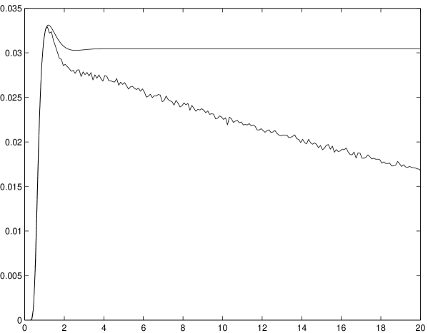
Figure 1: Plots of the function $W_{1}(t|0)$ and of the simulated FPT density $\tilde{g}(t)$ for a zero-mean stationary Gaussian process originating at $x_{0}=0$ having covariance (5.1) with $a=\omega=1$ and for the constant boundary $S(t)=2$.

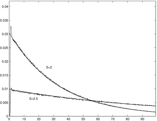
Figure 2: For the boundaries $S(t)\equiv S_{0}=2$ and $S(t)\equiv S_{0}=2.5$, the asymptotic exponential approximation $R(S_{0})\,\exp\{-R(S_{0})\,t\}$ and the simulated FPT density $\tilde{g}(t)$ are plotted for the Gaussian process of Figure 1.

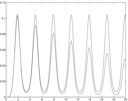
Figure 3: Same as in Figure 1 for the periodic boundary $S(t)=2+0.5\,\sin(2\,\pi\,t/3)$.

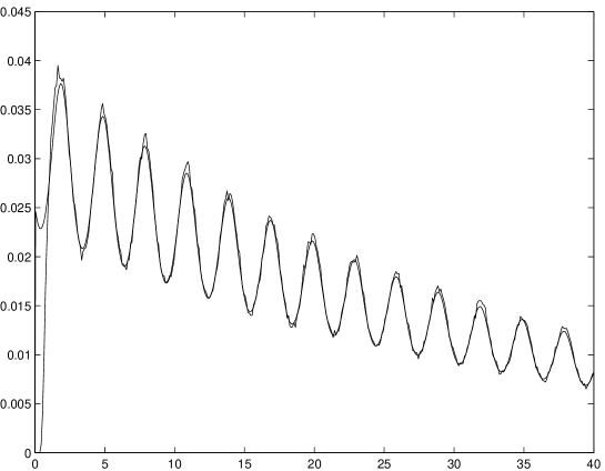
Figure 4: For the same process as in Figure 1 and for $S(t)=2+0.1\,\sin(2\,\pi\,\,t/3)$, the function $R[Z(t)]\,\exp\{-\int_{0}^{t}R[Z(\tau)]\,d\tau\}$ is plotted together with the simulated FPT density $\tilde{g}(t)$.

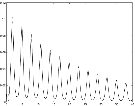
Figure 5: Same as in Figure 4 for the boundary $S(t)=2+0.5\,\sin(2\,\pi\,t/3)$.

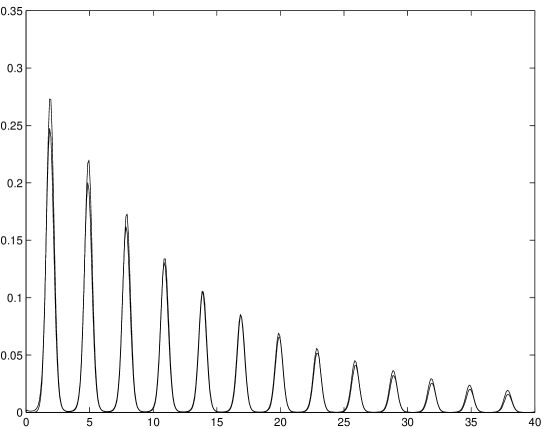
Figure 6: Same as in Figure 4 for the boundary $S(t)=2+\sin(2\,\pi\,t/3)$.

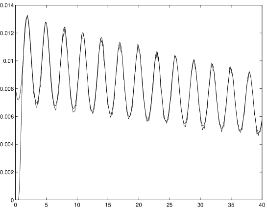
Figure 7: Same as in Figure 4 for the boundary $S(t)=2.5+0.1\,\sin(2\,\pi\,t/3)$.

5 Analysis of a special case

The purpose of this Section is to analyze the behavior of the FPT pdf for a stationary Gaussian process of concrete interest for certain applications.

Let $\left\{X(t),t\geq 0\right\}$ be the stationary Gaussian process originating at $x_{0}=0$, with zero mean and damped oscillatory covariance [32]:

$$\gamma(t)=e^{-a\,|t|}\,\Bigl{[}\cos\bigl{(}\omega\,t)+{a\over\omega}\,\sin\bigl{(}\omega\cdot|t|)\Bigr{]}\qquad(t\in{\bf R}),$$ (5.1)

where $a$ and $\omega$ are positive real numbers. Functions of form (5.1) can often be conveniently used to approximate experimental covariance functions that, starting from a unit initial maximum amplitude, asymptotically tend to zero with an exponential envelope. From (5.1) we see that $\gamma(0)=1$. Furthermore, $\dot{\gamma}(0)=0$ and $\ddot{\gamma}(0)=-(a^{2}+\omega^{2})<0$ since for $t>0$ there holds:

$$\dot{\gamma}(t)=-\dot{\gamma}(-t)=-{e^{-a\,t}\over\omega}\,(a^{2}+\omega^{2})\,\sin(\omega\,t),$$

(5.2)

$$\ddot{\gamma}(t)=\ddot{\gamma}(-t)={e^{-a\,t}\over\omega}\,(a^{2}+\omega^{2})\,\Bigl{[}a\,\sin(\omega\,t)-\omega\,\cos(\omega\,t)\Bigr{]}.$$

We finally note that $\lim\limits_{t\to+\infty}\gamma(t)=0$, $\lim\limits_{t\to+\infty}\dot{\gamma}(t)=0$ and $\lim\limits_{t\to+\infty}\ddot{\gamma}(t)=0$.

5.1 Constant boundary

For the constant boundary $S(t)=S_{0}$, from (3.4) one has

$$R(S_{0})={\sqrt{a^{2}+\omega^{2}}\over 2\,\pi}\;e^{\displaystyle{-S_{0}^{2}/2}}.$$ (5.3)

All forthcoming figures refer to the case $a=\omega=1$ in (5.1). Figure 1 shows the plots of $W_{1}(t|x_{0})$ given by (2.22) and of the simulated FPT density $\tilde{g}(t)$ as functions of $t$ for the constant boundary $S(t)=2$. The first-order approximation $W_{1}(t|x_{0})$ is seen to provide an upper bound to the FPT pdf in (2.21), being a good approximation of $g$ only for small values of $t$. From (3.4) it follows that, as $t$ increases, $W_{1}(t|x_{0})$ approaches the constant value $R(2)=e^{-2}/(\pi\,\sqrt{2})=0.0304611$. Making use of (3.21), we expect that $R(S_{0})\,\exp\{-R(S_{0})\,t\}$ provides a good approximation of the simulated FPT density $\tilde{g}(t)$ as $S_{0}\to+\infty$. Indeed, Figure 2 shows the plots of the simulated FPT density $\tilde{g}(t)$ for the constant boundary $S(t)\equiv S_{0}=2$ and of the function $R(2)\,\exp\{-R(2)\,t\}$. Figure 2 also shows the plots of the simulated FPT density $\tilde{g}(t)$ for the constant boundary $S(t)\equiv S_{0}=2.5$ and the function $R(2.5)\,\exp\{-R(2.5)\,t\}$ with $R(2.5)=e^{-3.125}/(\pi\,\sqrt{2})=0.00988928$. We note that starting from rather small times, $\tilde{g}(t)$ is susceptible of an excellent exponential approximation already for positive boundaries of the order of a couple of units.

5.2 Periodic boundary

For the same stationary Gaussian process, we now assume that $S(t)=S_{0}+B\,\sin(2\,\pi\,t/Q)$. In this case $Z(t)\equiv\varrho(t)=B\,\sin(2\,\pi\,t/Q)$ and condition (4.3) is satisfied. From (4.4) one has:

$$R[Z(t)]={\sqrt{a^{2}+\omega^{2}}\over 2\,\pi}\exp\biggl{\{}-{S^{2}(t)\over 2}\biggr{\}}\,\biggl{[}\exp\biggl{\{}-{[\dot{Z}(t)]^{2}\over 2\,(a^{2}+\omega^{2})}\biggr{\}}$$

$$\hskip 113.81102pt-\sqrt{{\pi\over 2\,(a^{2}+\omega^{2})}}\,\dot{Z}(t)\,{\rm Erfc}\,\biggl{(}{\dot{Z}(t)\over\sqrt{2\,(a^{2}+\omega^{2})}}\biggr{)}\biggr{]}.$$ (5.4)

From Remark 4.1 it follows that the function (5.4) is positive and periodic with period $Q$.

Figure 3 shows the plots of $W_{1}(t|0)$ and of the simulated FPT density $\tilde{g}(t)$ for the periodic boundary $S(t)=2+0.5\,\sin(2\,\pi\,t/3)$. We note again that the first-order approximation $W_{1}$ provides an upper bound to the FPT pdf given by (2.21), though being a good approximation of $g$ only for small values of $t$. Furthermore, as $k$ increases $W_{1}(t+k\,Q\,|\,0)$ tends to the function (5.4), i.e. as $t$ increases $W_{1}(t|0)$ becomes periodic with the same period of the boundary. Since

$$\lim_{S_{0}\to+\infty}\;{\varrho\biggl{(}\varphi\biggl{(}{\displaystyle{t\over\alpha}}\biggr{)}\biggr{)}\over S_{0}+Z\biggl{(}\varphi\biggl{(}{\displaystyle{t\over\alpha}}\biggr{)}\biggr{)}}=\lim_{S_{0}\to+\infty}\;{B\,\sin\Bigl{(}2\,\pi\,{\displaystyle{\varphi(t/\alpha)\over Q}}\Bigr{)}\over S_{0}+B\,\sin\Bigl{(}2\,\pi\,{\displaystyle{\varphi(t/\alpha)\over Q}}\Bigr{)}}=0,$$

condition (4.22) is satisfied, and thus the asymptotic formula (4.38) holds.

Figures 4$\div$7 show the plots of the simulated FPT density $\tilde{g}(t)$ for the periodic boundary $S(t)=S_{0}+B\,\sin(2\,\pi\,t/Q)$ and of the function $R[Z(t)]\,$ $\exp\{-\int_{0}^{t}R[Z(\tau)]\,d\tau\}$, with $R[Z(t)]$ given in (5.4) for various choices of parameters $S_{0}$, $B$ and $Q$. Figure 4 refers to the case $S_{0}=2$, $B=0.1$ and $Q=3$, Figure 5 to $S_{0}=2$, $B=0.5$ and $Q=3$, Figure 6 to $S_{0}=2$, $B=1$ and $Q=3$ and Figure 7 to $S_{0}=2.5$, $B=0.1$ and $Q=3$. Note that already from rather small times, $\tilde{g}(t)$ is susceptible of an excellent non-homogeneous exponential approximation.

6 Concluding Remarks

Gaussian processes play an important role in numerous fields. Although many of their properties have been deeply analyzed, very little exists in the literature concerning the first-passage-time probability density function in the presence of constant or time-varying boundaries, which would be suitable to make predictions on a variety of systems evolving in the presence of some critical regions of their state-space.

In the present paper, starting from some existing contributions to this problem area, for a class of stationary Gaussian processes it has been proved that a non-homogeneous exponential approximation holds for the first passage time probability density function in the presence of boundaries that either possess a horizontal asymptote or are asymptotically periodic. Furthermore, for a stationary Gaussian process with zero mean and with damped oscillatory covariance originating at $x_{0}=0$, extensive simulations have indicated that the FPT pdf $\tilde{g}(t)$ is susceptible of an excellent non-homogeneous exponential approximation for either constant or periodic boundaries, even though these are not very distant from the initial value of the process.

We trust that such results may prove useful for the description of the time evolution of systems characterized, for instance, by relaxation times much smaller than the mean observation times, thus making particularly appropriate and effective the asymptotic approximation obtained in the foregoing.

Appendix A Appendix I

Here we prove relations (3.15), (3.16), (3.17) and (3.18) of Theorem 3.1.

Recalling the first of (2.20) and making use of (3.1) we have:

$$\lim_{S_{0}\to+\infty}\dot{\psi}\left(\vartheta_{i}\right)=\lim_{S_{0}\to+\infty}\left[\dot{\varrho}\left(\vartheta_{i}\right)-x_{0}\,\dot{\gamma}\left(\vartheta_{i}\right)\right]=0\qquad(i=1,2,\ldots,n),$$

where the zero limit follows from (3.2), (3.7), (3.8) and (3.13). This proves (3.15).

By virtue of (3.7) and (3.8), and recalling (3.13), from (2.16) one has

$$\lim_{S_{0}\to+\infty}\lambda_{i+1,j+1}\left(\vartheta_{1},\ldots,\vartheta_{n}\right)=\left\{\begin{array}[]{cl}1,&i=j=0,\ldots,n\\ -\ddot{\gamma}(0),&i=j=n+1,\ldots,2n\\ 0,&i\neq j.\end{array}\right.$$ (A.4)

Hence, as $S_{0}\to+\infty$ the matrix $\Lambda_{2n+1}\left(\vartheta_{1},\ldots,\vartheta_{n}\right)$ becomes diagonal with the first $n+1$ elements equal to unity and the last $n$ elements equal to $-\ddot{\gamma}(0)$. Therefore, (3.16) holds.

To prove (3.17), we first notice that

$$\lim_{S_{0}\to+\infty}l_{i+1,j+1}\left(\vartheta_{1},\ldots,\vartheta_{n}\right)=\left\{\begin{array}[]{ll}[-\ddot{\gamma}(0)]^{n},&i=j=0,\ldots,n\\ \left[-\ddot{\gamma}(0)\right]^{n-1},&i=j=n+1,\ldots,2n\\ 0,&i\neq j.\end{array}\right.$$ (A.8)

Therefore, by making use of (3.16) and (A.8), from the second of (2.20) one obtains

$$\lim_{S_{0}\to+\infty}H\left(\vartheta_{1},\ldots,\vartheta_{n};\xi_{1},\ldots,\xi_{n}\right)$$

$$\hskip 28.45274pt=\lim_{S_{0}\to+\infty}\exp\biggl{\{}-{1\over 2\left|\Lambda_{2n+1}(\vartheta_{1},\ldots,\vartheta_{n})\right|}\sum_{i,j=1}^{n}l_{i+n+1,j+n+1}(\vartheta_{1},\ldots,\vartheta_{n})\,\xi_{i}\,\xi_{j}\biggr{\}}$$

$$\hskip 28.45274pt=\exp\left\{-{1\over 2\,[-\ddot{\gamma}(0)]}\sum_{i=1}^{n}\xi_{i}^{2}\right\},$$

so that (3.17) follows.

Finally, we prove (3.18). Recalling the last of (2.20) and (3.4), one obtains

$${1\over\bigl{[}R(S_{0})\bigr{]}^{n}}\,K\left(\vartheta_{1},\ldots,\vartheta_{n};\xi_{1},\ldots,\xi_{n}\right)={(2\pi)^{n}\over[-\ddot{\gamma}(0)]^{n/2}}$$ (A.9)

$$\times\exp\Biggl{\{}{n\,S_{0}^{2}\over 2}-{S_{0}^{2}\over 2\left|\Lambda_{2n+1}(\vartheta_{1},\ldots,\vartheta_{n})\right|}\biggl{[}\,\sum_{i,j=1}^{n}l_{i+1,j+1}(\vartheta_{1},\ldots,\vartheta_{n})\,{\psi(\vartheta_{i})\over S_{0}}\,{\psi(\vartheta_{j})\over S_{0}}$$

$$\hskip 2.84544pt+\sum_{i,j=1}^{n}l_{i+1,j+n+1}(\vartheta_{1},\ldots,\vartheta_{n})\,{\psi(\vartheta_{i})\over S_{0}^{2}}\,\xi_{j}+\sum_{i,j=1}^{n}l_{i+n+1,j+1}(\vartheta_{1},\ldots,\vartheta_{n})\,{\psi(\vartheta_{j})\over S_{0}^{2}}\,\xi_{i}\biggr{]}\Biggr{\}}.$$

We note that from the first of (2.20) and from (3.1), for $i=1,2,\ldots,n$ one has

$$\lim_{S_{0}\to+\infty}{\psi(\vartheta_{i})\over S_{0}}=\lim_{S_{0}\to+\infty}{S(\vartheta_{i})-x_{0}\gamma(\vartheta_{i})\over S_{0}}=\lim_{S_{0}\to+\infty}\Bigl{[}{S_{0}+\varrho(\vartheta_{i})\over S_{0}}-x_{0}\,{\gamma(\vartheta_{i})\over S_{0}}\Bigr{]}=1,$$ (A.10)

where the unit value follows from (3.2) , (3.7), (3.8), (3.9) and (3.13). Taking the limit as $S_{0}\to+\infty$ in (A.9), and making use of (3.16), (A.8) and (A.10), we finally obtain (3.18).

Appendix B Appendix II

Here we prove relations (4.31), (4.32) and (4.33) of Theorem 4.1.

By virtue of (3.8), (4.27) and (iv) of Proposition 4.3, relation (A.4) again follows from (2.16). Hence, as $S_{0}\to+\infty$ the matrix $\Lambda_{2n+1}\left(\vartheta_{1},\ldots,\vartheta_{n}\right)$ becomes diagonal with the first $n+1$ elements equal to unity and the last $n$ elements equal to $-\ddot{\gamma}(0)$, so that one immediately obtains (4.31).

The proof of (4.32) is analogous to the proof of (3.17) of Theorem 3.1, taking in account (4.27) and (iv) of Proposition 4.3.

Finally, we prove (4.33). Recalling the last of (2.20), one has

$$\exp\biggl{\{}{1\over 2}\sum\limits_{i=1}^{n}\bigl{[}S_{0}+Z\bigl{(}\vartheta_{i}\bigr{)}\bigr{]}^{2}\biggr{\}}\,K\left(\vartheta_{1},\ldots,\vartheta_{n};\xi_{1},\ldots,\xi_{n}\right)$$ (B.1)

$$=\exp\Biggl{\{}{S_{0}^{2}\over 2}\sum\limits_{i=1}^{n}\biggl{[}{S_{0}+Z\bigl{(}\vartheta_{i}\bigr{)}\over S_{0}}\biggr{]}^{2}-{S_{0}^{2}\over 2\left|\Lambda_{2n+1}(\vartheta_{1},\ldots,\vartheta_{n})\right|}$$

$$\times\biggl{[}\,\sum_{i,j=1}^{n}l_{i+1,j+1}(\vartheta_{1},\ldots,\vartheta_{n})\,{\psi(\vartheta_{i})\over S_{0}+Z\bigl{(}\vartheta_{i}\bigr{)}}\;{S_{0}+Z\bigl{(}\vartheta_{i}\bigr{)}\over S_{0}}\;{\psi(\vartheta_{j})\over S_{0}+Z\bigl{(}\vartheta_{j}\bigr{)}}\;{S_{0}+Z\bigl{(}\vartheta_{j}\bigr{)}\over S_{0}}$$

$$\hskip 14.22636pt+\sum_{i,j=1}^{n}l_{i+1,j+n+1}(\vartheta_{1},\ldots,\vartheta_{n})\,{\psi(\vartheta_{i})\over S_{0}+Z\bigl{(}\vartheta_{i}\bigr{)}}\;{S_{0}+Z\bigl{(}\vartheta_{i}\bigr{)}\over S_{0}^{2}}\;\;\xi_{j}$$

$$\hskip 14.22636pt+\sum_{i,j=1}^{n}l_{i+n+1,j+1}(\vartheta_{1},\ldots,\vartheta_{n})\,{\psi(\vartheta_{j})\over S_{0}+Z\bigl{(}\vartheta_{j}\bigr{)}}\;{S_{0}+Z\bigl{(}\vartheta_{j}\bigr{)}\over S_{0}^{2}}\;\;\xi_{i}\biggr{]}\Biggr{\}}.$$

Moreover,

$$\lim_{S_{0}\to+\infty}{S_{0}+Z\bigl{(}\vartheta_{i}\bigr{)}\over S_{0}}=1\qquad(i=1,2,\ldots,n),$$ (B.2)

since $Z(t)$ is a bounded function independent of $S_{0}$. Furthermore, we note that from the first of (2.20) and from (4.1), for $i=1,2,\ldots,n$ one obtains

$$\lim_{S_{0}\to+\infty}{\psi(\vartheta_{i})\over S_{0}+Z\bigl{(}\vartheta_{i}\bigr{)}}=\lim_{S_{0}\to+\infty}{S(\vartheta_{i})-x_{0}\,\gamma(\vartheta_{i})\over S_{0}+Z\bigl{(}\vartheta_{i}\bigr{)}}$$

$$\hskip 85.35826pt=\lim_{S_{0}\to+\infty}\Bigl{[}{S_{0}+\varrho(\vartheta_{i})\over S_{0}+Z\bigl{(}\vartheta_{i}\bigr{)}}-x_{0}\;{\gamma(\vartheta_{i})\over S_{0}+Z\bigl{(}\vartheta_{i}\bigr{)}}\Bigr{]}=1,$$ (B.3)

where the last equality follows by using condition (iii) of Proposition 4.3 and by recalling (3.8), (4.2) and (4.22). Taking the limit as $S_{0}\to+\infty$ in (B.1), and making use of (3.16), (A.8), (B.2) and (B.3), one thus obtains (4.33).

References

- [1] Abramowitz, M. and Stegun, I.A., Handbook of Mathematical Functions, Dover Publications Inc., New York, 1972.
- [2] Anderssen, R.S., DeHoog, F.R. and Weiss R., “On the numerical solution of Brownian motion processes,” J. Appl. Prob., vol. 10, 409–418, 1973.
- [3] Buonocore, A., Nobile, A.G. and Ricciardi, L.M., “A new integral equation for the evaluation of first-passage-time probability densities,” Adv. Appl. Prob., vol. 19, 784–800, 1987.
- [4] Buonocore, A., Giorno, V., Nobile, A.G. and Ricciardi, L.M., “On the two-boundary first-crossing-time problem for diffusion processes,” J. Appl. Prob., vol. 27, 102–114, 1990.
- [5] Daniels, H.E., “Approximating the first crossing-time density for a curved boundary,” Bernoulli, vol 2, (2), 133–143, 1996.
- [6] Daniels, H.E., “The first crossing-time density for Brownian motion with a perturbed linear boundary,” Bernoulli, vol. 6, (4), 571–580, 2000.
- [7] Di Crescenzo, A., Giorno, V., Nobile, A.G. and Ricciardi, L.M., “On first-passage-time and transition densities for strongly symmetric diffusion processes,” Nagoya Math. J., vol 145, 143–161, 1997.
- [8] Di Crescenzo, A., Di Nardo, E., Nobile, A.G., Pirozzi, E. and Ricciardi, L.M., “On some computational results for single neurons’ activity modeling,” BioSystems, vol. 58, 19–26, 2000.
- [9] Di Nardo, E., Pirozzi, E., Ricciardi, L.M. and Rinaldi, S., “Vectorized simulations of normal processes for first crossing-time problems,” Lecture Notes in Computer Science, vol. 1333, 177–188, 1997.
- [10] Di Nardo, E., Nobile, A.G., Pirozzi, E., Ricciardi, L.M., and Rinaldi, S., “Simulation of Gaussian processes and first passage time densities evaluation,” Lecture Notes in Computer Science, vol. 1798, 319–333, 2000.
- [11] Di Nardo, E., Nobile, A.G., Pirozzi, E. and Ricciardi, L.M., “A computational approach to first-passage-time problems for Gauss-Markov processes,” Adv. Appl. Prob., vol. 33, pp. 453–482, 2001.
- [12] Di Nardo, E., Nobile, A.G., Pirozzi, E. and Ricciardi, L.M., “Computer-aided simulations of Gaussian processes and related asymptotic properties,” Lecture Notes in Computer Science, vol. 2178, 67–78,2001.
- [13] Durbin, J., “Boundary-crossing probabilities for the brownian motion and Poisson processes and techniques for computing the power of the Kolmogorov-Smirnov test,” J. Appl. Prob. vol 8, 431–453, 1971.
- [14] Durbin, J., “The first-passage density of a continuous gaussian process to a general boundary,” J. Appl. Prob., vol. 22, 99–122, 1985.
- [15] Ferebee, B., “The tangent approximation to one-sided Brownian exit densities,” Z. Wahrscheinlichkeitsth, vol. 61, 309–326, 1982.
- [16] Giorno, V., Nobile, A.G. and Ricciardi, L.M., “A new approach to the construction of first-passage-time densities” in Proceeding of 9th European Congress on Cybernetics and Systems Research (R. Trappl, ed.), Kluwer Academic Publishers, 375–381, 1988.
- [17] Giorno, V., Nobile, A.G. ,Ricciardi, L.M. and Sato, S., “On the evaluation of first-passage-time densities via nonsingular integral equations, ” Adv. Appl. Prob., vol. 21, 20–36, 1989.
- [18] Giorno, V., Nobile, A.G. and Ricciardi, L.M., “A symmetry-based constructive approach to probability densities for one dimensional diffusion processes,” J. Appl. Prob., vol. 27, 707–721, 1989.
- [19] Giorno, V., Nobile, A.G. and Ricciardi, L.M., “On the asymptotic behavior of first-passage-time densities for one-dimensional diffusion processes and varying boundaries,” Adv. Appl. Prob., vol. 22, 883–914, 1990.
- [20] Gutiérrez, R., Ricciardi, L.M., Román, P. and Torres, F., “First-passage-time densities for time-non-homogeneous diffusion processes,” J. Appl. Prob., vol. 34, 623–631, 1997.
- [21] Kostyukov, A.I., Ivanov, Y.N. and Kryzhanovsky, M.V., “Probability of neuronal spike initiation as a curve-crossing problem for gaussian stochastic processes,” Biol. Cybern., vol. 39, 157–163, 1981.
- [22] Lánský, P. and Sato, S., “The stochastic diffusion models of nerve membrane depolarization and interspike interval generation,” J. of the Peripheral Nervous System, vol. 4, 27–42, 1999.
- [23] Nobile, A.G., Ricciardi, L.M. and Sacerdote, L., “Exponential trends of Ornstein-Uhlenbeck first passage time densities,” J. Appl. Prob., vol. 22, 360–369, 1985.
- [24] Nobile, A.G., Ricciardi, L.M. and Sacerdote, L., “Exponential trends of first-passage-time densities for a class of diffusion processes with steady-state distribution,” J. Appl. Prob., vol. 22, 611–618, 1985.
- [25] Ricciardi, L.M., Diffusion Processes and Related Topics in Biology, Springer-Verlag, New York, 1977.
- [26] Ricciardi, L.M. and Sato, S., “A note on first passage time for Gaussian processes and varying boundaries,” IEEE Transactions on Information Theory, vol. 29, 454–457, 1983.
- [27] Ricciardi, L.M. and Sato, S., “On the evaluation of first-passage-time densities for Gaussian processes,” Signal Processing, vol. 11, 339–357, 1986.
- [28] Ricciardi, L.M., Di Crescenzo, A., Giorno, V. and Nobile, A.G., “An outline of theoretical and algorithmic approaches to first passage time problems with applications to biological modeling,” Math. Japonica, vol. 50,(2), 247–322, 1999.
- [29] Roberts, J.B., “An approach to the first-passage problems in random vibration,” J. Sound Vib., vol. 8,(2), 301–328, 1968.
- [30] Sacerdote, L., “Asymptotic behavior of Ornstein–Uhlenbeck first-passage-time density through periodic boundaries,” Applied Stochastic Models and Data Analysis, vol. 6, 53–57, 1988.
- [31] Sato, S., “Evaluation of first-passage time probability to a square root boundary for the Wiener process,” J. Appl. Prob., vol. 14, 850–856, 1977.
- [32] Stratonovich, R.L., Topics in the Theory of Random Noise, vol. 1, Gordon & Breach Publishing Group, 1963.