Uniform bounds on multigraded regularity

Abstract.

We give an effective uniform bound on the multigraded regularity of a subscheme of a smooth projective toric variety $X$ with a given multigraded Hilbert polynomial. To establish this bound, we introduce a new combinatorial tool, called a Stanley filtration, for studying monomial ideals in the homogeneous coordinate ring of $X$. As a special case, we obtain a new proof of Gotzmann’s regularity theorem. We also discuss applications of this bound to the construction of multigraded Hilbert schemes.

1. Introduction

Bounding the degree of the generators of a module or sheaf is a central problem in commutative algebra and algebraic geometry. The modern approach to this problem concentrates on proving stronger bounds involving Castelnuovo-Mumford regularity. In fact, Castelnuovo-Mumford regularity was introduced in §14 of [Mum] to bound the family of all projective subschemes having a given Hilbert polynomial. Following this appearance, Castelnuovo-Mumford regularity has become a crucial ingredient in bounding the degree of syzygies [GLP] [EL] and constructing Hilbert schemes, Picard schemes and moduli spaces [AK] [Vie].

The goal of this paper is to bound the multigraded Castelnuovo-Mumford regularity (as defined in [MS]) of all subschemes of a smooth projective toric variety $X$ that have a given multigraded Hilbert polynomial. To establish this bound, we work with saturated monomial ideals in the homogeneous coordinate ring of $X$. We introduce a new combinatorial tool, called a Stanley filtration, for studying monomial ideals. Using an appropriate Stanley filtration, we produce an effective bound for the multigraded regularity of an individual ideal or family of ideals. We also discuss applications of our bound to the construction of multigraded Hilbert schemes.

Using ideals in the homogeneous coordinate ring $S$ to analyze subschemes of $X$ has several advantages. The $\mathbb{Z}^{r}$-graded polynomial ring $S=\Bbbk[x_{1},\dotsc,x_{n}]$, introduced in [Cox1], is intrinsic to the variety $X$. By focusing on $X$ rather than a projective embedding of $X$, we reduce both the number of variables and the total degree of the polynomials needed to describe a subscheme. When $\operatorname{Pic}(X)\neq\mathbb{Z}$, the multigrading allows for stronger bounds on the equations defining a subscheme. Multigradings also produce a finer stratification of subschemes of $X$.

The novel approach required for multigraded polynomial rings leads to new insights in the standard graded case. Indeed, when $X=\mathbb{P}^{d}$, we obtain a new proof of Gotzmann’s optimal bound on the regularity of all subschemes having a given Hilbert polynomial. Gotzmann’s original proof [Got] relies on Macaulay’s characterization of the Hilbert function of an ideal in a standard graded polynomial ring. Since there is no version of Macaulay’s theorem for nonstandard gradings, the methods used in [Got] do not apply in our situation. In fact, there is typically no lexicographic ideal in the homogeneous coordinate ring of $X$ (see [ACD]) so we cannot expect a direct analogy of Macaulay’s result. The alternative proof of Gotzmann’s result given in [Gre1], also see [Gre2] and §4.3 in [BH], uses an induction on a general hyperplane section. Because a general hypersurface is rarely a toric variety, this approach does not extend to toric varieties.

The main combinatorial tool used in this paper is based on a Stanley decomposition. Given a monomial ideal $I$ in $S$, a Stanley decomposition for $S/I$ is a set $\mathfrak{S}$ of pairs $(\bm{x}^{\bm{u}},\sigma)$ such that $S/I\cong\bigoplus\nolimits_{(\bm{x}^{\bm{u}},\sigma)\in\mathfrak{S}}S_{\sigma}\bigl{(}-\deg(\bm{x}^{\bm{u}})\bigr{)}$, where $\bm{x}^{\bm{u}}$ is a monomial in $S$, $\sigma\subseteq\{1,\dotsc,n\}$ and $S_{\sigma}=\Bbbk[x_{i}:i\in\sigma]$. In other words, if we identify the pair $(\bm{x}^{\bm{u}},\sigma)$ with the set $\{\bm{x}^{\bm{u}+\bm{v}}\in S:\bm{x}^{\bm{v}}\in S_{\sigma}\}$, then each monomial of $S$ not in $I$ belongs to a unique pair $(\bm{x}^{\bm{u}},\sigma)$. It follows that a Stanley decomposition expresses the multigraded Hilbert polynomial of $S/I$ as a sum of the Hilbert polynomials for $S_{\sigma}$:

(1.0.1) $$P_{S/I}(\bm{t})=\sum_{(\bm{x}^{\bm{u}},\sigma)\in\mathfrak{S}}P_{S_{\sigma}}\bigl{(}\bm{t}-\deg(\bm{x}^{\bm{u}})\bigr{)}\,.$$

Example 1.1.

Let $S=\Bbbk[x_{1},\dotsc,x_{4}]$ have standard grading defined by $\deg(x_{i})=1$ for $1\leq i\leq 4$. If $I=\langle x_{1}x_{4}^{2},x_{2}x_{4}^{2},x_{3}x_{4}^{2}\rangle$ is an ideal in $S$ then

$$\bigl{\{}(1,\{1,2,3\}),(x_{4},\{1,2,3\}),(x_{4}^{2},\{4\})\bigr{\}}$$ and

$$\bigr{\{}(1,\{4\}),(x_{3},\{3\}),(x_{3}x_{4},\{4\}),(x_{2},\{2,3\}),(x_{2}x_{4},\{2,3\}),(x_{1},\{1,2,3\}),(x_{1}x_{4},\{1,2,3\})\bigr{\}}$$

are both Stanley decompositions for $S/I$. Since the Hilbert polynomial $P_{S_{\sigma}}(t)$ is simply the binomial coefficient $\binom{t+|\sigma|-1}{|\sigma|+1}$, these Stanley decompositions yield

$$P_{S/I}(t) =\textstyle\binom{t+2}{2}+\binom{t+1}{2}+\binom{t-2}{0}$$

$$=\textstyle\binom{t}{0}+\binom{t-1}{0}+\binom{t-2}{0}+\binom{t}{1}+\binom{t-1}{1}+\binom{t+1}{2}+\binom{t}{2}\,.$$

We focus on a particular class of Stanley decompositions called Stanley filtrations. By definition, these are ordered sets $\{(\bm{x}^{\bm{u}_{i}},\sigma_{i}):1\leq i\leq m\}$ such that the modules $M_{j}=S/\bigl{(}I+\langle\bm{x}^{\bm{u}_{j+1}},\dotsc,\bm{x}^{\bm{u}_{m}}\rangle\bigr{)}$ form a filtration $\Bbbk=M_{0}\subset M_{1}\subset\dotsb\subset M_{m}=S/I$ with $M_{i}/M_{i-1}=S_{\sigma_{i}}$. The decompositions of Example 1.1 are Stanley filtrations in the order presented. We provide an algorithm for finding Stanley filtrations.

Our first major theorem uses a Stanley filtration to give an effective bound on the multigraded regularity. Recall that bounding the multigraded regularity of a module $M$ is equivalent to giving a subset of $\operatorname{reg}(M)=\bigl{\{}\bm{k}\in\mathbb{Z}^{r}:\text{$M$ is $\bm{k}$-regular}\bigr{\}}$. For more information on multigraded regularity, we refer to [MS]. Remarkably, our major theorems use only the behavior of multigraded regularity in short exact sequences and hence are independent of the precise definition of multigraded regularity.

Theorem 4.1.

Let $I$ be a monomial ideal in $S$. If $\bigl{\{}(\bm{x}^{\bm{u}_{i}},\sigma_{i}):1\leq i\leq m\bigr{\}}$ is a Stanley filtration for $S/I$, then $\bigcap_{i=1}^{m}\bigl{(}\deg(\bm{x}^{\bm{u}_{i}})+\operatorname{reg}(S_{\sigma_{i}})\bigr{)}\subseteq\operatorname{reg}\left(S/I\right)$.

By relating the sets $\sigma_{i}$ to the fan $\Delta$ defining $X$, we can eliminate certain pairs from this intersection.

Example 1.2.

Since $\operatorname{reg}(S)=\mathbb{N}$ for any standard graded polynomial ring, the first Stanley filtration in Example 1.1 implies that

$$\max\{\deg(1),\deg(x_{4}),\deg(x_{4}^{2})\}+\mathbb{N}\subseteq\operatorname{reg}(S/I)\,.$$

The minimal free resolution of $S/I$ shows that this bound is sharp: $\operatorname{reg}(S/I)=\bm{2}+\mathbb{N}$.

To study all subschemes of $X$ with a given multigraded Hilbert polynomial, we use the combinatorial structure of $\Delta$ to focus on a finite set of Stanley filtrations. We also concentrate on ideals that are saturated with respect to the irrelevant ideal $B$; see Section 2. Given a polynomial $P(\bm{t})$, we are most interested in expressions of the form (1.0.1) arising from our finite set of Stanley filtrations. This leads to an algorithm for finding all $B$-saturated monomial ideals with multigraded Hilbert polynomial $P(\bm{t})$. We call the maximum number of summands in such an expression for $P(\bm{t})$ the Gotzmann number.

To state our second major result, let $\widehat{\sigma}$ denote the complement of $\sigma$ in $\{1,\dotsc,n\}$. Identifying $\operatorname{Pic}(X)$ with $\mathbb{Z}^{r}$, we write $\bm{\mathcal{K}}\subset\mathbb{Z}^{r}$ for the semigroup of nef line bundles on $X$; see Section 2 for a combinatorial description of $\bm{\mathcal{K}}$.

Theorem 4.11.

Let $I$ be any $B$-saturated ideal in $S$ and let $\bm{c}\in\bigcap_{i=1}^{n}\bigl{(}\deg(x_{i})+\bm{\mathcal{K}}\bigr{)}$. If $m$ is the Gotzmann number for $P_{S/I}(\bm{t})$ then $\bigcap\limits_{\widehat{\sigma}\in\Delta}\bigl{(}(m-1)\bm{c}+\operatorname{reg}(S_{\sigma})\bigr{)}\subseteq\operatorname{reg}(S/I)$.

This theorem implies that for any $\bm{k}\in\bigcap\nolimits_{\widehat{\sigma}\in\Delta}\bigl{(}(m-1)\bm{c}+\operatorname{reg}(S_{\sigma})\bigr{)}$ every the subscheme of $X$ having multigraded Hilbert polynomial $P_{S/I}(\bm{t})$ is cut out by equations of multidegree $\bm{k}$. Specializing to $X=\mathbb{P}^{d}$, we recover Gotzmann’s regularity theorem; see Theorem 5.2.

The structure of the paper is as follows. The next section establishes our notation for toric varieties, recalls the definition of multigraded regularity from [MS] and collects the basic properties of multigraded Hilbert polynomials. In Section 3, we develop the theory of Stanley decompositions and filtrations. The proofs of our major theorems are in Section 4. This section also contains the algorithm for finding all $B$-saturated monomial ideals with a given multigraded Hilbert polynomial. In Section 5, we restrict to the case $X=\mathbb{P}^{d}$ and show that multigraded techniques provide a simple new proof of Gotzmann’s regularity theorem. Finally, Section 6 discusses the effective construction of multigraded Hilbert schemes.

Acknowledgements.

We thank Ezra Miller for the references on cleanness. We also thank Kristina Crona and Edwin O’Shea for their helpful comments on a preliminary version of this paper. Both authors were partially supported by the Mathematical Sciences Research Institute in Berkeley, CA.

2. Castelnuovo-Mumford Regularity and Hilbert Polynomials

This section relates multigraded Hilbert polynomials to multigraded Castelnuovo-Mumford regularity (as defined in [MS]). Let $X$ be a smooth projective toric variety over a field $\Bbbk$ determined by a fan $\Delta$ in $\mathbb{R}^{d}$. By numbering the rays (one-dimensional cones), we identify $\Delta$ with a simplicial complex on $[n]:=\{1,\dotsc,n\}$. We write $\bm{b}_{1},\dotsc,\bm{b}_{n}$ for the unique minimal lattice vectors generating the rays and we assume that $\bm{b}_{1},\dotsc,\bm{b}_{n}$ span $\mathbb{R}^{d}$. Set $r:=n-d$ and fix an $(r\times n)$-matrix $A=[\bm{a}_{1}\dotsb\bm{a}_{n}]$ such that there is a short exact sequence

(2.0.2) $$0\longrightarrow\mathbb{Z}^{d}\xrightarrow{\;[\bm{b}_{1}\dotsb\,\bm{b}_{n}]^{\textsf{T}}\;}\mathbb{Z}^{n}\xrightarrow{\;[\bm{a}_{1}\dotsb\,\bm{a}_{n}]\;}\mathbb{Z}^{r}\longrightarrow 0\,.$$

Because $A$ is the Gale dual of the $(d\times n)$-matrix $[\bm{b}_{1}\dotsb\bm{b}_{n}]$, it is uniquely determined up to unimodular (determinant $\pm 1$) coordinate transformations of $\mathbb{Z}^{r}$. Since $X$ is smooth, the Picard group of $X$ is isomorphic to $\mathbb{Z}^{r}$. The homogeneous coordinate ring of $X$, introduced in [Cox1], is the polynomial ring $S=\Bbbk[x_{1},\dotsc,x_{n}]$ with the $\mathbb{Z}^{r}$-grading defined by $\deg(x_{i})=\bm{a}_{i}\in\mathbb{Z}^{r}$ for $1\leq i\leq n$. The combinatorial structure of $\Delta$ is encoded in the irrelevant ideal $B=\bigl{\langle}\prod_{i\not\in\sigma}x_{i}:\sigma\in\Delta\bigr{\rangle}$. With these definitions, [Cox1] proves that the category of coherent $\mathscr{O}_{X}$-modules is equivalent to the category of finitely generated $\mathbb{Z}^{r}$-graded $S$-modules modulo $B$-torsion modules.

Example 2.1.

When $X=\mathbb{P}^{d}$, the short exact sequence (2.0.2) is

$$0\longrightarrow\mathbb{Z}^{d}\longrightarrow\mathbb{Z}^{d+1}\xrightarrow{\;[1\;1\,\dotsb\,1]\;}\mathbb{Z}^{1}\longrightarrow 0\,.$$

Since $\deg(x_{i})=\bm{a}_{i}=1$ for $1\leq i\leq n=d+1$, the homogeneous coordinate ring $S=\Bbbk[x_{1},\dotsc,x_{n}]$ is simply the standard graded polynomial ring. The irrelevant ideal $B$ is the unique graded maximal ideal $\langle x_{1},\dotsc,x_{n}\rangle$.

Example 2.2.

If $X$ is the Hirzebruch surface (or rational scroll) $\mathbb{F}_{\ell}=\mathbb{P}\big{(}\mathscr{O}_{\mathbb{P}^{1}}\oplus\mathscr{O}_{\mathbb{P}^{1}}(\ell)\big{)}$, then the short exact sequence (2.0.2) is

$$0\longrightarrow\mathbb{Z}^{2}\xrightarrow{\;\left[\begin{smallmatrix}1&0&-1&0\\ 0&1&\ell&-1\end{smallmatrix}\right]^{\textsf{T}}\;}\mathbb{Z}^{4}\xrightarrow{\;\left[\begin{smallmatrix}1&-\ell&1&0\\ 0&1&0&1\end{smallmatrix}\right]\;}\mathbb{Z}^{2}\longrightarrow 0\,.$$

Figure 1 illustrates the fan and grading $A$ when $\ell=2$.

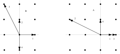
Figure 1. The fan and grading for $\mathbb{F}_{2}$.

The homogeneous coordinate ring $S=\Bbbk[x_{1},x_{2},x_{3},x_{4}]$ has the $\mathbb{Z}^{2}$-grading induced by $\deg(x_{1})=\left[\begin{smallmatrix}1\\ 0\end{smallmatrix}\right]$, $\deg(x_{2})=\left[\begin{smallmatrix}-\ell\\ 1\end{smallmatrix}\right]$, $\deg(x_{3})=\left[\begin{smallmatrix}1\\ 0\end{smallmatrix}\right]$, $\deg(x_{4})=\left[\begin{smallmatrix}0\\ 1\end{smallmatrix}\right]$ and $B=\langle x_{1}x_{2},x_{2}x_{3},x_{3}x_{4},x_{1}x_{4}\rangle=\langle x_{1},x_{3}\rangle\cap\langle x_{2},x_{4}\rangle$.

The combinatorial structure of $\Delta$ also gives rise to an important subsemigroup of $\mathbb{Z}^{r}$. We write $\mathbb{N}A_{\sigma}:=\{\sum_{i\in\sigma}\lambda_{i}\bm{a}_{i}:\lambda_{i}\in\mathbb{N}\}$ for the affine semigroup generated by the set $\{\bm{a}_{i}:i\in\sigma\}$. For $\sigma\subseteq[n]$, let $\widehat{\sigma}$ denote the complement of $\sigma$ in $[n]$. The semigroup $\bm{\mathcal{K}}$ is $\bigcap_{\sigma\in\Delta}\mathbb{N}A_{\widehat{\sigma}}$. Since $X$ is projective, $\bm{\mathcal{K}}$ is the set of integral points of an $r$-dimensional pointed cone in $\mathbb{R}^{r}$. Geometrically, elements in $\bm{\mathcal{K}}$ correspond to numerically effective (nef) line bundles on $X$. As [Cox2] indicates, $\bm{\mathcal{K}}\otimes_{\mathbb{Z}}\mathbb{R}$ is the closure of the Kähler cone of $X$. The dual of the Kähler cone is the Mori cone of effective $1$-cycles modulo numerical equivalence.

Example 2.3.

When $X=\mathbb{P}^{d}$, the semigroup $\bm{\mathcal{K}}=\mathbb{N}$. If $X=\mathbb{F}_{\ell}$ (with $A$ chosen as in Example 2.2), then $\bm{\mathcal{K}}=\mathbb{N}^{2}$. In general, the structure of $\bm{\mathcal{K}}$ can be much more complicated; see Example 2.8 in [MS].

The next result illustrates the connection between the irrelevant ideal $B$ and the semigroup $\bm{\mathcal{K}}$. For $\sigma\subseteq[n]$, let $P_{\sigma}$ be the prime ideal $\langle x_{i}:i\not\in\sigma\rangle$ and let $S_{\sigma}$ be the (smaller) polynomial ring $\Bbbk[x_{i}:i\in\sigma]\cong S/P_{\sigma}$.

Lemma 2.4.

A monomial ideal $I$ in $S$ is $B$-saturated if and only if every associated prime $P_{\sigma}$ of $I$ satisfies $\widehat{\sigma}\in\Delta$ $($or equivalently $\bm{\mathcal{K}}\subseteq\mathbb{N}A_{\sigma})$.

Proof.

Let $I=\bigcap_{\sigma}Q_{\sigma}$ be an irredundant primary decomposition for $I$ where the ideal $Q_{\sigma}$ is $P_{\sigma}$-primary. It follows that $(I:B^{\infty})=\bigcap_{\sigma}(Q_{\sigma}:B^{\infty})=\bigcap_{\sigma}\bigcap_{\tau\in\Delta}\bigl{(}Q_{\sigma}:(\prod_{i\not\in\tau}x_{i})^{\infty}\bigr{)}$. Now $\bigl{(}Q_{\sigma}:(\prod_{i\not\in\tau}x_{i})^{\infty}\bigr{)}$ equals $S$ if $\widehat{\sigma}\cap\widehat{\tau}\neq\emptyset$ and equals $Q_{\sigma}$ otherwise. Since $\widehat{\sigma}\cap\widehat{\tau}=\emptyset$ is equivalent to $\widehat{\sigma}\subseteq\tau$, we have $(I:B^{\infty})=\bigcap_{\widehat{\sigma}\in\Delta}Q_{\sigma}$. Therefore, $(I:B^{\infty})=I$ if and only if every associated prime $P_{\sigma}$ satisfies $\widehat{\sigma}\in\Delta$. The equivalent condition follows immediately from the definition of $\bm{\mathcal{K}}$. ∎

Throughout this paper, $M$ denotes a finitely generated $\mathbb{Z}^{r}$-graded $S$-module. We refer to [BS] for background information on local cohomology. The module $M$ is $B$-torsion if $M=H_{B}^{0}(M)=\bigcup_{j\in\mathbb{N}}(0:_{M}B^{j})$. At the other extreme, $M$ is $B$-torsion-free if $H_{B}^{0}(M)=0$. For an ideal $I\subseteq S$, the module $S/I$ is $B$-torsion-free if and only if $I$ is $B$-saturated; $(I:B^{\infty})=I$.

Remark 2.5.

The semigroup $\bm{\mathcal{K}}$ also has a useful algebraic interpretation. If $\Bbbk$ is infinite and $M$ is $B$-torsion-free, then Proposition 3.1 in [MS] shows that for any $\bm{k}\in\bm{\mathcal{K}}$ there is a nonzerodivisor $f\in S_{\bm{k}}$ on $M$.

Let $\bm{\mathcal{C}}=\{\bm{c}_{1},\dotsc,\bm{c}_{e}\}$ be the unique minimal Hilbert basis of $\bm{\mathcal{K}}$. By definition, $\bm{\mathcal{C}}$ is the minimal subset of $\bm{\mathcal{K}}$ such that every element in $\bm{\mathcal{K}}$ is a nonnegative integral combination of the $\bm{c}_{j}$; see § ​​IV.16.4 in [Sch]. We recall the definition of multigraded Castelnuovo-Mumford regularity introduced in [MS].

Definition 2.6.

For $\bm{k}\in\mathbb{Z}^{r}$, the module $M$ is $\bm{k}$-regular if the following conditions are satisfied:

1. $H_{B}^{i}(M)_{\bm{p}}=0$ for all $i\geq 1$ and all $\bm{p}\in\bigcup(\bm{k}-\lambda_{1}\bm{c}_{1}-\dotsb-\lambda_{e}\bm{c}_{e}+\bm{\mathcal{K}})$ where the union is over all $\lambda_{1},\dotsc,\lambda_{e}\in\mathbb{N}$ such that $\lambda_{1}+\dotsb+\lambda_{e}=i-1$;

2. $H_{B}^{0}(M)_{\bm{p}}=0$ for all $\bm{p}\in\bigcup_{1\leq j\leq e}(\bm{k}+\bm{c}_{j}+\bm{\mathcal{K}})$.

The regularity of $M$, denoted by $\operatorname{reg}(M)$, is the set $\{\bm{k}\in\mathbb{Z}^{r}:\text{$M$ is $\bm{k}$-regular}\}$.

In this paper, we exploit two properties of multigraded Castelnuovo-Mumford regularity. Firstly, if $I$ is an ideal in $S$ and $\bm{k}\in\operatorname{reg}(I)$ then the subscheme of $X$ defined by $I$ is cut out by equations of multidegree $\bm{k}$; see Theorem 6.9 in [MS]. The second property allows us to focus on monomial ideals by relating the regularity of an ideal with its initial ideal. We write $\operatorname{in}(I)$ for the initial ideal of $I$ with respect to some monomial order. The following proposition, which is well-known for $X=\mathbb{P}^{d}$, appears as Proposition 6.13 in [MS].

Proposition 2.7.

If $I$ is an ideal in $S$, then $\operatorname{reg}\bigl{(}S/\operatorname{in}(I)\bigr{)}\subseteq\operatorname{reg}(S/I)$. Moreover, if $I$ is $B$-saturated and $J=\bigl{(}\operatorname{in}(I):B^{\infty}\bigr{)}$ then $\operatorname{reg}(S/J)\subseteq\operatorname{reg}(S/I)$. ∎

Next, we turn our attention to multigraded Hilbert polynomials. The multigraded Hilbert function $H(M,\bm{t})$ equals the dimension of the degree $\bm{t}$ homogeneous component of a $\mathbb{Z}^{r}$-graded module $M$. As in the standard graded case, $H(M,\bm{t})$ “eventually” agrees with a polynomial. To prove this, we first consider the multigraded Hilbert function of the ring $S$.

Lemma 2.8.

If $S$ is the coordinate ring of a smooth toric variety then the Hilbert function $H(S,\bm{t})=\dim_{\Bbbk}S_{\bm{t}}$ agrees with a polynomial for all $\bm{t}\in\bm{\mathcal{K}}$.

Proof.

Since the monomials of degree $\bm{t}$ form a basis for the $\Bbbk$-vector space $S_{\bm{t}}$, the Hilbert function $H(S,\bm{t})$ is a vector partition function. This means $H(S,\bm{t})$ equals the number of ways a vector $\bm{t}\in\mathbb{Z}^{r}$ can be written as a sum of $\bm{a}_{1},\dotsc,\bm{a}_{n}$. The chamber complex of $\{\bm{a}_{1},\dotsc,\bm{a}_{n}\}$ is a polyhedral subdivision of $\operatorname{pos}\{\bm{a}_{1},\dotsc,\bm{a}_{n}\}$. It is defined to be the common refinement of the simplicial cones $\operatorname{pos}\{\bm{a}_{i}:i\not\in\sigma\}$ where $\sigma\in\Delta$. Hence, the cone $\bm{\mathcal{K}}\otimes_{\mathbb{Z}}\mathbb{R}$ is a chamber (maximal cell) in the chamber complex. From [St1], we know that vector partition functions are piecewise quasi-polynomials on the chamber complex. Therefore, $H(S,\bm{t})$ is a quasi-polynomial on $\bm{\mathcal{K}}$.

To complete the proof, we show that the period of this quasi-polynomial is one. We write $[\bm{a}_{i}:i\not\in\sigma]$ for the submatrix of $A$ consisting of those columns indexed by $\sigma$. From [St1], we know that the period of the quasi-polynomial is at most the least common multiple of $\det[\bm{a}_{i}:i\not\in\sigma]$ where $\sigma$ is a facet in $\Delta$. By renumbering (if necessary) the $\bm{b}_{i}$, we may assume that $\sigma=\{1,\dotsc,d\}\in\Delta$. Recall that $X$ is smooth if and only if $\det[\bm{b}_{i}:i\in\sigma]=\pm 1$ for all facets $\sigma\in\Delta$; see §2.1 in [Ful]. Hence, there exists a unimodular change of coordinates such that $\bm{b}_{i}=\bm{e}_{i}$ for all $i\in\sigma$ where $\bm{e}_{i}$ is the $i$th standard basis vector. In other words, $[\bm{b}_{1}\dotsb\bm{b}_{n}]$ is the block matrix $[I_{d}\,|\,V_{\sigma}]$ where $V_{\sigma}$ is a $(d\times r)$-matrix. The Gale dual of this configuration is $[V_{\sigma}^{\textsf{T}}\,|\,-I_{r}]$. Because the Gale dual is determined up to unimodular transformation, we have $\det[\bm{a}_{i}:i\not\in\sigma]=\pm\det[I_{r}]=\pm 1$ for all facets $\sigma\in\Delta$. ∎

Algorithms for computing $P_{S}(\bm{t})$ have been implemented in the software package LattE; see [LHTY].

Example 2.9.

When $X=\mathbb{P}^{d}$, we have $P_{S}(t)=\binom{t+d}{d}$. If $X=\mathbb{F}_{\ell}$, then we have $P_{S}(t_{1},t_{2})=t_{1}t_{2}+\bigl{(}\tfrac{\ell}{2}\bigr{)}t_{2}^{2}+t_{1}+\bigl{(}\tfrac{\ell+2}{2}\bigr{)}t_{2}+1$.

Using Lemma 2.8, we show that the multigraded Hilbert function of a module $M$ agrees with a polynomial for values of $\bm{t}$ sufficiently far into the interior of $\bm{\mathcal{K}}$.

Proposition 2.10.

There exists a unique polynomial $P_{M}(\bm{t})\in\mathbb{Q}[t_{1},\dotsc,t_{r}]$ such that $P_{M}(\bm{t})=H(M,\bm{t})$ for all $\bm{t}$ in a finite intersection of translates of $\bm{\mathcal{K}}$. In particular, $H(M,\bm{t})$ agrees with $P_{M}(\bm{t})$ for all $\bm{t}$ sufficiently far from the boundary of $\bm{\mathcal{K}}$.

Proof.

If $0\longrightarrow\bigoplus_{j}S(-\bm{q}_{p,j})\longrightarrow\dotsb\longrightarrow\bigoplus_{j}S(-\bm{q}_{0,j})$ is the minimal free resolution of $M$, then $H(M,\bm{t})=\sum_{i=0}^{p}\sum_{j}(-1)^{i}H(S,\bm{t}-\bm{q}_{i,j})$. It follows from Lemma 2.8 that $H(M,\bm{t})$ is a polynomial for all $\bm{t}\in\bigcap_{i,j}(\bm{q}_{i,j}+\bm{\mathcal{K}})$. Since $\bm{q}_{i,j}\in\mathbb{Z}^{r}$ and $\bm{\mathcal{K}}$ corresponds to the lattice points in an $r$-dimensional cone in $\mathbb{R}^{r}$, this intersection is nonempty. ∎

Definition 2.11.

The polynomial $P_{M}(\bm{t})$ in Proposition 2.10 is called the multigraded Hilbert polynomial of $M$.

The multigraded Hilbert polynomial of a $B$-torsion module is especially simple.

Lemma 2.12.

If $M$ is a $B$-torsion module then $P_{M}(\bm{t})=0$.

Proof.

Since $M$ is a finitely generated $B$-torsion module, there is a $j\gg 0$ such that $B^{j}M=0$. We first prove that there exists a $\bm{k}\in\bm{\mathcal{K}}$ such that if $\bm{p}\in\bm{k}+\bm{\mathcal{K}}$ then every monomial in $S_{\bm{p}}$ belongs to $B^{j}$. Choose an element $\bm{c}$ which lies in the interior of $\bm{\mathcal{K}}$. If $\bm{x}^{\bm{u}}$ is a monomial in $S$ and $\deg(\bm{x}^{\bm{u}})\in\bm{c}+\bm{\mathcal{K}}$, then Lemma 2.4 in [MS] shows that $\bm{x}^{\bm{u}}\in B$. Suppose that $\bm{x}^{\bm{v}}\in S$ such that $\deg(\bm{x}^{\bm{v}})=n\bm{c}+\bm{c}^{\prime}$ for $\bm{c}^{\prime}\in\bm{\mathcal{K}}$. Caratheodory’s Theorem (Proposition 1.15 in [Zie]) implies that $\bm{v}=\lambda_{1}\bm{u}_{1}+\dotsb+\lambda_{n}\bm{u}_{n}+\bm{w}$ for some $\bm{u}_{1},\dotsc,\bm{u}_{n}\in\mathbb{N}^{n}$ satisfying $\deg(\bm{x}^{\bm{u}_{i}})=\bm{c}$ for $1\leq i\leq n$, $\bm{w}\in\mathbb{R}_{\geq 0}^{n}$ satisfying $A\bm{w}=\bm{c}^{\prime}$ and some $\lambda_{1},\dotsc,\lambda_{n}\in\mathbb{R}_{\geq 0}$ satisfying $\lambda_{1}+\dotsb+\lambda_{n}=n$. It follows that there is an $i\in[n]$ such that $\lambda_{i}\geq 1$ and hence $\bm{x}^{\bm{v}}$ is divisible by $\bm{x}^{\bm{u}_{i}}$. Therefore, if we set $\bm{k}:=(j+n)\bm{c}$ then $\deg(\bm{x}^{\bm{v}})\in\bm{k}+\bm{\mathcal{K}}$ implies that $\bm{x}^{\bm{v}}\in B^{j}$.

To complete the proof, we show that $M_{\bm{t}}=0$ for all $\bm{t}$ sufficiently far into the interior of $\bm{\mathcal{K}}$. Let $f_{1},\dotsc,f_{h}$ be generators of $M$. Our choice of $\bm{k}$ guarantees that $M_{\bm{t}}=0$ for all $\bm{t}\in\bigcap_{1\leq i\leq h}\bigl{(}\deg(f_{i})+\bm{k}+\bm{\mathcal{K}}\bigr{)}$. Since elements in $\bm{\mathcal{K}}$ are lattice points in a full-dimensional cone, the elements in this intersection are the lattice points in a translation of the same cone. We conclude that $P_{M}(\bm{t})=0$. ∎

More generally, the multigraded Hilbert polynomial of a module is independent of $B$-torsion.

Lemma 2.13.

If $\overline{M}:=M/H_{B}^{0}(M)$ then $P_{M}(\bm{t})=P_{\overline{M}}(\bm{t})$. In particular, if $I\subseteq S$ is an ideal then $S/I$ and $S/(I:B^{\infty})$ have the same Hilbert polynomial.

Proof.

Since $H_{B}^{0}(M)$ is a $B$-torsion module, Lemma 2.12 shows that its multigraded Hilbert polynomial equals $0$. Hence, the short exact sequence

$$0\longrightarrow H_{B}^{0}(M)\longrightarrow M\longrightarrow\overline{M}\longrightarrow 0$$

implies that $P_{M}(\bm{t})=P_{\overline{M}}(\bm{t})$. Because $H_{B}^{0}(S/I)=(I:B^{\infty})/I$, the second assertion is a special case of the first part. ∎

The following result connects Hilbert functions with local cohomology modules. The special case in which $S$ has the standard grading can be found in §4.4 of [BH].

Proposition 2.14.

We have

(2.14.3) $$H(M,\bm{t})-P_{M}(\bm{t})=\sum_{i=0}^{d}(-1)^{i}\dim_{\Bbbk}H_{B}^{i}(M)_{\bm{t}}\qquad\text{for all $\bm{t}\in\mathbb{Z}^{r}$.}$$

Proof.

We proceed by induction on $\dim M$. If $\dim M=0$, then $M$ is artinian. Hence, $M$ is a $B$-torsion module and we have $M=H_{B}^{0}(M)$ and $H_{B}^{i}(M)=0$ for all $i\geq 1$. Since Lemma 2.12 shows that $P_{M}(\bm{t})=0$, the assertion follows.

Assume $\dim M>0$. Since both sides of (2.14.3) change by $\dim_{\Bbbk}H_{B}^{0}(M)_{\bm{t}}$ when $M$ is replaced by $M/H_{B}^{0}(M)$, we may assume that $M$ is $B$-torsion-free. Because extension of the base field commutes with the formation of local cohomology, we may also assume that $\Bbbk$ is infinite. Choose $\bm{k}\in\bm{\mathcal{K}}$. Remark 2.5 implies there is a nonzerodivisor $f$ on $M$ with $f\in S_{\bm{k}}$. Hence, $\dim M/fM<\dim M$ and there is a short exact sequence

(2.14.4) $$0\longrightarrow M(-\bm{k})\xrightarrow{\;\;f\;\;}M\longrightarrow M/fM\longrightarrow 0\,.$$

Set $H_{M}^{\prime}(\bm{z})=\sum\nolimits_{\bm{t}\in\mathbb{Z}^{r}}\big{(}H(M,\bm{t})-P_{M}(\bm{t})\big{)}\,\bm{z}^{\bm{t}}$ and

$$H_{M}^{\prime\prime}(\bm{z})=\sum_{\bm{t}\in\mathbb{Z}^{r}}\left(\sum_{i=0}^{d}(-1)^{i}\dim_{\Bbbk}H_{B}^{i}(M)_{\bm{t}}\right)\bm{z}^{\bm{t}}\,.$$

With this notation, it suffices to prove that $H_{M}^{\prime}(\bm{z})=H_{M}^{\prime\prime}(\bm{z})$. From (2.14.4), it follows that $H(M/fM,\bm{t})=H(M,\bm{t})-H(M,\bm{t}-\bm{k})$. Combining this with Proposition 2.10, we deduce that $P_{M/fM}(\bm{t})=P_{M}(\bm{t})-P_{M}(\bm{t}-\bm{k})$ for all $\bm{t}$ sufficiently far into the interior of $\bm{\mathcal{K}}$ and thus for all $\bm{t}$. Hence, we have $H_{M/fM}^{\prime}(\bm{z})=(1-\bm{z}^{\bm{k}})H_{M}^{\prime}(\bm{z})$. On the other hand, the long exact sequence associated to (2.14.4) shows that

$$\sum_{i=0}^{d}(-1)^{i}\dim_{\Bbbk}H_{B}^{i}(M/fM)_{\bm{t}}=\sum_{i=0}^{d}(-1)^{i}\bigl{(}\dim_{\Bbbk}H_{B}^{i}(M)_{\bm{t}}-\dim_{\Bbbk}H_{B}^{i}(M)_{\bm{t}-\bm{k}}\bigr{)}\,.$$

Therefore, we have $H_{M/fM}^{\prime\prime}(\bm{z})=(1-\bm{z}^{\bm{k}})H_{M}^{\prime\prime}(\bm{z})$. Since the induction hypothesis yields $H_{M/fM}^{\prime}(\bm{z})=H_{M/fM}^{\prime\prime}(\bm{z})$, we conclude that $H_{M}^{\prime}(\bm{z})=H_{M}^{\prime\prime}(\bm{z})$. ∎

Corollary 2.15.

If $M$ is $\bm{k}$-regular then the Hilbert function $H(M,\bm{t})$ agrees with the Hilbert polynomial $P_{M}(\bm{t})$ for all values $\bm{t}\in\bm{k}+\bm{\mathcal{K}}$ with $\bm{t}\neq\bm{k}$.

Proof.

If $M$ is $\bm{k}$-regular, then $H_{B}^{i}(M)_{\bm{t}}=0$ for all $i\geq 0$ and all $\bm{t}\in\bm{k}+\bm{\mathcal{K}}$ with $\bm{t}\neq\bm{k}$. Hence, the claim follows from Proposition 2.14. ∎

Multigraded Hilbert polynomials also have a geometric description, which is attributed to Snapper in [Kle]. Let $\mathscr{O}_{X}(\bm{t})$ be the line bundle on $X$ corresponding to $\bm{t}\in\mathbb{Z}^{r}$ and let $\mathscr{F}$ be the $\mathscr{O}_{X}$-module associated to the $S$-module $M$. Since equation (6.3.1) in [MS] indicates that

$$\dim_{\Bbbk}H^{0}\bigl{(}X,\mathscr{F}\otimes\mathscr{O}_{X}(\bm{t})\bigr{)}=H(M,\bm{t})-\dim_{\Bbbk}H_{B}^{0}(M)_{\bm{t}}+\dim_{\Bbbk}H_{B}^{1}(M)_{\bm{t}}\,,$$

Proposition 2.14 implies that

$$P_{M}(\bm{t})=\chi\bigl{(}\mathscr{F}\otimes\mathscr{O}_{X}(\bm{t})\bigr{)}=\sum\limits_{i=1}^{d}(-1)^{i}\dim H^{i}\bigl{(}X,\mathscr{F}\otimes\mathscr{O}_{X}(\bm{t})\bigr{)}\,.$$

For a finite set of points, the connection between multigraded regularity and multigraded Hilbert polynomials is particularly elegant.

Example 2.16.

Let $I$ be the $B$-saturated ideal corresponding to a finite set of points on $X$. Proposition 6.7 in [MS] shows that $\operatorname{reg}(S/I)$ is exactly the subset of $\mathbb{Z}^{r}$ for which the Hilbert function $H(S/I,\bm{t})$ equals the Hilbert polynomial $P_{S/I}(\bm{t})$.

3. Stanley Decompositions and Filtrations

In this section we introduce the key combinatorial tool used in this paper. We restrict our focus to a monomial ideal $I$ in the polynomial ring $S$, and introduce the notion of a Stanley decomposition for $S/I$. This is a partition of the monomials of $S$ not in $I$ into sets each of which corresponds to the monomials in a smaller polynomial ring.

Definition 3.1.

If $\bm{x}^{\bm{u}}\in S$ and $\sigma\subseteq[n]$, the pair $(\bm{x}^{\bm{u}},\sigma)$ denotes the set of all monomials in $S$ of the form $\bm{x}^{\bm{v}+\bm{u}}$ where $\operatorname{supp}(\bm{v}):=\{i:v_{i}\neq 0\}\subseteq\sigma$. A Stanley decomposition for $S/I$ is a set $\mathfrak{S}$ of pairs $(\bm{x}^{\bm{u}},\sigma)$ such that

$$S/I\cong\bigoplus_{(\bm{x}^{\bm{u}},\sigma)\in\mathfrak{S}}S_{\sigma}(-A\bm{u})\,,$$

where $S_{\sigma}:=\Bbbk[x_{i}:i\in\sigma]$. In other words, each monomial of $S$ not in $I$ belongs to a unique pair $(\bm{x}^{\bm{u}},\sigma)$ in the Stanley decomposition.

A Stanley decomposition $\mathfrak{S}$ for $S/I$ also gives a primary decomposition of $I$:

$$I=\bigcap_{(\bm{x}^{\bm{u}},\sigma)\in\mathfrak{S}}\langle x_{i}^{u_{i}+1}:i\not\in\sigma\rangle\,.$$

This is typically not the unique irreducible irredundant primary decomposition of $I$. Stanley decompositions are inspired by [Sta] and algorithmically defined in [SW]; also see [HTh], [Ape]. Both [Sta] and [Ape] require the extra condition that $|\sigma|$ should be at least the depth of $I$.

Example 3.2.

If $I=\langle x_{1}^{2}x_{2},x_{1}x_{2}^{2}\rangle\subset S=\Bbbk[x_{1},x_{2}]$, then

1. $\bigl{\{}\bigl{(}1,\{1\}\bigr{)},\bigl{(}x_{2},\{2\}\bigr{)},\bigl{(}x_{1}x_{2},\emptyset\bigr{)}\bigr{\}}$,

2. $\bigl{\{}\bigl{(}1,\{2\}\bigr{)},\bigl{(}x_{1},\{1\}\bigr{)},\bigl{(}x_{1}x_{2},\emptyset\bigr{)}\bigr{\}}$ and

3. $\bigl{\{}\bigl{(}1,\emptyset\bigr{)},\bigl{(}x_{1},\{1\}\bigr{)},\bigl{(}x_{2},\emptyset\bigr{)},\bigl{(}x_{2}^{2},\{2\}\bigr{)},\bigl{(}x_{1}x_{2},\emptyset\bigr{)}\bigr{\}}$

are three distinct Stanley decomposition for $S/I$. These are illustrated in Figure 2.

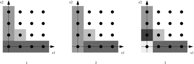
Figure 2. Stanley decompositions for $\langle x_{1}^{2}x_{2},x_{1}x_{2}^{2}\rangle$.

Stanley decompositions are closely related to standard pairs. See [STV] for the origin of the notation $(\bm{x}^{\bm{u}},\sigma)$ and more details. Standard pairs enjoy the following property: if $(\bm{x}^{\bm{u}},\sigma)$ is a standard pair of $I$ then $P_{\sigma}=\langle x_{i}:i\not\in\sigma\rangle$ is an associated prime of $I$. In contrast, not all ideals have a Stanley decomposition where every $\sigma$ corresponds to an associated prime.

Example 3.3.

If $I=\langle x_{1},x_{2}\rangle\cap\langle x_{3},x_{4}\rangle=\langle x_{1}x_{3},x_{1}x_{4},x_{2}x_{3},x_{2}x_{4}\rangle$ is a monomial ideal in the ring $S=\Bbbk[x_{1},x_{2},x_{3},x_{4}]$, then $\bigl{\{}\bigl{(}1,\{1,2\}\bigr{)},\bigl{(}x_{4},\{4\}\bigr{)},\bigl{(}x_{3},\{3,4\}\bigr{)}\bigr{\}}$ is a Stanley decomposition for $S/I$ where $\{4\}$ does not correspond to an associated prime of $I$. One easily verifies for this ideal that every Stanley decomposition for $S/I$ has a pair $(\bm{x}^{\bm{u}},\sigma)$ for which $\sigma$ does not correspond to an associated prime.

The paper [Sim] studies the special case when $S/I$ has a Stanley decomposition in which each $\sigma$ corresponds to a minimal associated prime of $I$. Decompositions with this property are called clean.

One way to construct a Stanley decomposition is to make repeated use of the short exact sequence

(3.3.5) $$0\longrightarrow S(-\bm{a}_{i})/(I:x_{i})\xrightarrow{\;\;x_{i}\;\;}S/I\longrightarrow S/(I+\langle x_{i}\rangle)\longrightarrow 0\,,$$

where $x_{i}$ is any variable. More explicitly, we have following algorithm. A special case of this algorithm is implicit in the proof of Lemma 2.4 in [SW].

Algorithm 3.4.

Given a monomial ideal $I$ in the polynomial ring $S$ with $I\neq S$, the following algorithm computes a Stanley decomposition for $S/I$.

1. (Base case) If $I$ is a prime ideal, then let $\sigma$ correspond to the set of variables not in $I$ and output $\bigl{\{}(1,\sigma)\bigr{\}}$.

2. (Choose variable) If $I$ is not prime then choose a variable $x_{\ell}\in S$ that is a proper divisor of a minimal generator of $I$.

3. (Recursion) Compute a Stanley decomposition $\bigl{\{}(\bm{x}^{\bm{u}},\tau)\bigr{\}}$ for $S/(I+\langle x_{\ell}\rangle)$ and a Stanley decomposition $\bigl{\{}(\bm{x}^{\bm{v}},\sigma)\bigr{\}}$ for $S/(I:x_{\ell})$. Output $\bigl{\{}(\bm{x}^{\bm{u}},\tau)\bigr{\}}\cup\bigl{\{}(\bm{x}^{\bm{v}}x_{\ell},\sigma)\bigr{\}}$.

Proof of Correctness.

A monomial ideal is prime if and only if it is generated by a subset of the variables. Hence, when $I$ is prime and $\sigma$ corresponds to the set of variables not in $I$, the set $\bigl{\{}(1,\sigma)\bigr{\}}$ is a Stanley decomposition for $S/I$. On the other hand, if $I$ is not prime, then there exists a variable $x_{\ell}$ that is a proper divisor of a minimal generator of $I$. From (3.3.5), we see that a monomial not in $I$ corresponds to either a monomial not in $S/(I+\langle x_{\ell}\rangle)$ or $x_{\ell}$ times a monomial not in $S/(I:x_{\ell})$. Thus, if $\bigl{\{}(\bm{x}^{\bm{u}},\tau)\bigr{\}}$ is a Stanley decomposition for $S/(I+\langle x_{\ell}\rangle)$ and $\bigl{\{}(\bm{x}^{\bm{v}},\sigma)\bigr{\}}$ is a Stanley decomposition for $S/(I:x_{i})$, then $\bigl{\{}(\bm{x}^{\bm{u}},\tau)\bigr{\}}\cup\bigl{\{}(\bm{x}^{\bm{v}}x_{\ell},\sigma)\bigr{\}}$ is a Stanley decomposition for $S/I$. Finally, the algorithm terminates because $S$ is a noetherian ring. Indeed, both $I+\langle x_{\ell}\rangle$ and $(I:x_{\ell})$ are strictly larger ideals than $I$, so non-termination would give an infinite chain of strictly increasing ideals. ∎

Remark 3.5.

Running Algorithm 3.4 generates a rooted binary tree. The nodes are monomial ideals and the root is the input ideal. At each node, Step 2 chooses a variable $x_{\ell}$. The left-hand child of a node $J$ is the ideal $J+\langle x_{\ell}\rangle$ and the right-hand child is $(J:x_{\ell})$. The corresponding branches are labeled with the monomials $1$ and $x_{\ell}$ respectively. The leaves of this tree are prime ideals and each leaf corresponds to an element in the Stanley decomposition. Specifically, a leaf corresponds to the pair $(\bm{x}^{\bm{u}},\sigma)$ where $\bm{x}^{\bm{u}}$ is the product of labels in the path from the root to the leaf and $\sigma$ corresponds to the variables not in the prime ideal. We will call such a tree the associated binary tree for the Stanley decomposition. These trees also appear in [Sim].

Example 3.6.

If $I=\langle x_{1}^{2}x_{2},x_{1}x_{2}x_{3},x_{2}^{2}x_{3},x_{1}^{2}x_{4},x_{1}x_{2}x_{4},x_{2}^{2}x_{4}\rangle\subset S=\Bbbk[x_{1},x_{2},x_{3},x_{4}]$, then the Stanley decomposition

$$\bigl{\{}\bigl{(}1,\{3,4\}\bigr{)},\bigl{(}x_{2},\{3,4\}\bigr{)},\bigl{(}x_{2}^{2},\{2\}\bigr{)},\bigl{(}x_{1},\{3,4\}\bigr{)},\bigl{(}x_{1}x_{2},\{2\}\bigr{)},\bigl{(}x_{1}^{2},\{1,3\}\bigr{)}\bigr{\}}$$

for $S/I$ produced by Algorithm 3.4 corresponds to the following binary tree.

These binary trees equip the Stanley decompositions produced by Algorithm 3.4 with an additional structure. To describe this structure, we introduce the following concept.

Definition 3.7.

A Stanley filtration is a Stanley decomposition with an ordering of the pairs $\bigl{\{}(\bm{x}^{\bm{u}_{i}},\sigma_{i}):1\leq i\leq m\bigr{\}}$ such that for all $1\leq j\leq m$ the set $\bigl{\{}(\bm{x}^{\bm{u}_{i}},\sigma_{i}):1\leq i\leq j\bigr{\}}$ is a Stanley decomposition for $S/\bigl{(}I+\langle\bm{x}^{\bm{u}_{j+1}},\dotsc,\bm{x}^{\bm{u}_{m}}\rangle\bigr{)}$. Equivalently, the ordered set is a Stanley filtration provided the modules $M_{j}=S/\bigl{(}I+\langle\bm{x}^{\bm{u}_{j+1}},\dotsc,\bm{x}^{\bm{u}_{m}}\rangle\bigr{)}$ form a filtration $\Bbbk=M_{0}\subset M_{1}\subset\dotsc\subset M_{m}=S/I$ with $M_{j}/M_{j-1}\cong S_{\sigma_{j}}$.

Example 3.8.

Not every Stanley decomposition has an ordering that makes it a Stanley filtration. For example, no ordering of the pairs in the Stanley decomposition

$$\bigl{\{}\bigl{(}1,\emptyset\bigr{)},\bigl{(}x_{1},\{1,2\}\bigr{)},\bigl{(}x_{2},\{2,3\}\bigr{)},\bigl{(}x_{3},\{1,3\}\bigr{)}\bigr{\}}$$

for $\Bbbk[x_{1},x_{2},x_{3}]/\langle x_{1}x_{2}x_{3}\rangle$ is a Stanley filtration.

If $S/I$ has a Stanley filtration in which each $\sigma_{i}$ corresponds to a minimal prime of the ideal $I$, then Corollary 2.2.4 in [Sim] implies that $S/I$ is Cohen-Macaulay.

A standard way to traverse the leaves of a rooted tree is via depth-first search where all left-hand descendants of a node are listed before any right-hand descendants. This corresponds to listing the leaves from left to right in the diagram of Example 3.6.

Corollary 3.9.

Let $I\subseteq S$ be a monomial ideal and let $\mathfrak{S}$ be a Stanley decomposition for $S/I$ obtained by applying Algorithm 3.4. If the pairs have the order induced by a depth-first search (starting with left-hand children) of the associated binary tree, then $\mathfrak{S}$ is a Stanley filtration.

Proof.

Let $\mathfrak{S}=\bigl{\{}(\bm{x}^{\bm{u}_{i}},\sigma_{i}):1\leq i\leq m\bigr{\}}$ and let $T$ be the binary tree associated to $\mathfrak{S}$. We write $L_{i}$ for the leaf corresponding to the pair $(\bm{x}^{\bm{u}_{i}},\sigma_{i})$. We assume that $i<j$ implies that a depth-first search of $T$ arrives at $L_{i}$ before reaching $L_{j}$. It suffices to show that the set $\bigl{\{}(\bm{x}^{\bm{u}_{i}},\sigma_{i}):1\leq i\leq m-1\bigr{\}}$ can be obtained by applying Algorithm 3.4 to $I+\langle\bm{x}^{\bm{u}_{m}}\rangle$. To accomplish this, we describe the binary tree $T^{\prime}$ generated by applying Algorithm 3.4 to $I+\langle\bm{x}^{\bm{u}_{m}}\rangle$. The tree $T^{\prime}$ is obtained from $T$ by deleting $L_{m}$ and contracting the branch joining the parent of $L_{m}$ with its left-hand child. The only nodes in $T^{\prime}$ that differ from $T$ are the first $|\bm{u}_{m}|$ nodes on the extreme right-hand branch. These ideals are obtained from those in $T$ by adding a proper divisor of $\bm{x}^{\bm{u}_{m}}$. ∎

Example 3.10.

The converse of Corollary 3.9 is false, as there are Stanley filtrations that do not arise from Algorithm 3.4. For example, the third Stanley decomposition in Example 3.2 is a Stanley filtration with respect to the given ordering that cannot be obtained from Algorithm 3.4. Indeed, any decomposition obtained from Algorithm 3.4 must have a term $(1,\{1\})$ or $(1,\{2\})$ because $I+\langle x_{i}\rangle=\langle x_{i}\rangle$ for $i=1$, $2$.

4. Bounds on Regularity

This section contains the main results of this paper. We first show how a Stanley filtration for $S/I$ leads to a bound on its multigraded regularity.

Theorem 4.1.

Let $I$ be a monomial ideal in $S$. If $\bigl{\{}(\bm{x}^{\bm{u}_{i}},\sigma_{i}):1\leq i\leq m\bigr{\}}$ is a Stanley filtration for $S/I$, then $\bigcap_{i=1}^{m}\bigl{(}A\bm{u}_{i}+\operatorname{reg}(S_{\sigma_{i}})\bigr{)}\subseteq\operatorname{reg}\left(S/I\right)$. In addition, if $I$ is $B$-saturated, then the intersection can be taken over those pairs $(\bm{x}^{\bm{u}_{i}},\sigma_{i})$ such that $\widehat{\sigma}_{i}\in\Delta$.

Proof.

Let $\bm{\mathcal{R}}^{0}(M):=\{\bm{k}\in\mathbb{Z}^{r}:\text{$H_{B}^{0}(M)_{\bm{k}+\bm{c}}=0$ for all $\bm{0}\neq\bm{c}\in\bm{\mathcal{K}}$}\}$ and for $j>0$ set $\bm{\mathcal{R}}^{j}(M):=\{\bm{k}\in\mathbb{Z}^{r}:\text{ $H_{B}^{j}(M)_{\bm{k}-\lambda_{1}\bm{c}_{1}-\dotsb-\lambda_{e}\bm{c}_{e}}=0$ for all $\lambda_{i}\in\mathbb{N}$ with $\sum\lambda_{i}=j-1$}\}$. With this notation, we have $\operatorname{reg}(S/I)=\bigcap_{j\geq 0}\bm{\mathcal{R}}^{j}(S/I)$. We claim that

(4.1.6) $$\bm{\mathcal{R}}^{j}(S/I)=\bigcap_{i=1}^{m}\bigl{(}A\bm{u}_{i}+\bm{\mathcal{R}}^{j}(S_{\sigma_{i}})\bigr{)}\,.$$

This implies the first part of the theorem. Additionally, if $I$ is $B$-saturated then $\bm{\mathcal{R}}^{0}(S/I)=\mathbb{Z}^{r}$ and $\operatorname{reg}(S/I)=\bigcap_{j>0}\bm{\mathcal{R}}^{j}(S/I)$. When $\widehat{\sigma}\not\in\Delta$, Lemma 2.4 implies that $S_{\sigma}=S/P_{\sigma}$ is a $B$-torsion module, so $H_{B}^{j}(S_{\sigma})=0$ for $j>0$. It follows that $\bm{\mathcal{R}}^{j}(S_{\sigma})=\mathbb{Z}^{r}$ for $j>0$ and hence $\bigcap_{i=1}^{m}\bigl{(}A\bm{u}_{i}+\bm{\mathcal{R}}^{j}(S_{\sigma_{i}})\bigr{)}=\bigcap_{\widehat{\sigma}_{i}\in\Delta}\bigl{(}A\bm{u}_{i}+\bm{\mathcal{R}}^{j}(S_{\sigma_{i}})\bigr{)}$. Therefore, the claim also establishes the second part of the theorem.

We prove (4.1.6) by induction on $m$. When $m=1$, the unique pair has the form $(1,\sigma)$ which implies that $I=P_{\sigma}=\langle x_{i}:i\not\in\sigma\rangle$ and $\bm{\mathcal{R}}^{j}(S/I)=\bm{\mathcal{R}}^{i}(S_{\sigma})$. Suppose that the claim holds for all Stanley filtrations with fewer than $m$ pairs. The short exact sequence $0\longrightarrow S(-A\bm{u}_{m})/(I:\bm{x}^{\bm{u}_{m}})\xrightarrow{\;\bm{x}^{\bm{u}_{m}}\;}{S}/{I}\longrightarrow{S}/(I+\langle\bm{x}^{\bm{u}_{m}}\rangle)\longrightarrow 0$ yields the exact sequence

(4.1.7) $$H_{B}^{j}\bigl{(}S/(I:\bm{x}^{\bm{u}_{m}})\bigr{)}_{\bm{p}-A\bm{u}_{m}}\longrightarrow H_{B}^{j}\bigl{(}S/I\bigr{)}_{\bm{p}}\longrightarrow H_{B}^{j}\bigl{(}S/(I+\langle\bm{x}^{\bm{u}_{m}}\rangle)\bigr{)}_{\bm{p}}\,.$$

From this, we deduce that $\bm{\mathcal{R}}^{j}\bigl{(}S/(I+\langle\bm{x}^{\bm{u}_{m}})\bigr{)}\cap\bigl{(}A\bm{u}_{m}+\bm{\mathcal{R}}^{j}\bigl{(}S/(I:\bm{x}^{\bm{u}_{m}})\bigr{)}\bigr{)}\subseteq\bm{\mathcal{R}}^{j}(S/I)$. Since $\bigl{\{}(\bm{x}^{\bm{u}_{i}},\sigma_{i}):1\leq i\leq m-1\bigr{\}}$ is a Stanley filtration for $S/(I+\langle\bm{x}^{\bm{u}_{m}}\rangle)$, the induction hypothesis implies that $\bm{\mathcal{R}}^{j}\bigl{(}S/(I+\langle\bm{x}^{\bm{u}_{m}}\rangle)\bigr{)}=\bigcap_{i=1}^{m-1}\bigl{(}A\bm{u}_{i}+\bm{\mathcal{R}}^{j}(S_{\sigma_{i}})\bigr{)}$. The ordering also implies that no monomial in $S$ divisible by $\bm{x}^{\bm{u}_{m}}$ belongs to the set $\bigcup_{i=1}^{m-1}(\bm{x}^{\bm{u}_{i}},\sigma_{i})$. It follows that a monomial $\bm{x}^{\bm{u}_{m}+\bm{v}}\in S$ is not contained in $I$ if and only if $\operatorname{supp}(\bm{v})\subseteq\sigma_{m}$. Therefore, we have $(I:\bm{x}^{\bm{u}_{m}})=P_{\sigma_{m}}$ and $\bm{\mathcal{R}}^{j}\bigl{(}S/(I:\bm{x}^{\bm{u}_{m}})\bigr{)}=\bm{\mathcal{R}}^{j}(S_{\sigma_{m}})$ which completes the induction. ∎

Remark 4.2.

If $S$ has the standard grading (equivalently $X=\mathbb{P}^{d}$), then Theorem 4.1 says that the Castelnuovo-Mumford regularity of a monomial ideal is bounded by the maximum of $|\bm{u}_{i}|:=\sum_{i=1}^{n}u_{i}$ for a Stanley filtration $\bigl{\{}(\bm{x}^{\bm{u}_{i}},\sigma_{i})\bigr{\}}$.

We next examine the relationship between Stanley filtrations and Hilbert polynomials. Given a Stanley filtration $\bigl{\{}(\bm{x}^{\bm{u}_{i}},\sigma_{i}):1\leq i\leq m\bigr{\}}$ for $S/I$, we have

$$H(S/I,\bm{t})=\sum_{i=1}^{m}H(S_{\sigma_{i}},\bm{t}-A\bm{u}_{i})\,.$$

Since $\bm{\mathcal{K}}\subseteq\mathbb{N}A_{\sigma}$ if and only if $\widehat{\sigma}\in\Delta$, the Hilbert polynomial of $S/I$ has an expression with potentially fewer summands: $P_{S/I}(\bm{t})=\sum_{\widehat{\sigma}\in\Delta}P_{S_{\sigma}}(\bm{t}-A\bm{u})$. To place further restrictions on the summands, we need an ordering on the $\widehat{\sigma}\in\Delta$.

We endow the polynomial ring $\mathbb{Q}[t_{1},\dotsc,t_{r}]$ with the $\mathbb{Z}$-grading defined by $\deg(t_{i})=1$ for $1\leq i\leq r$. Let $<$ be a monomial order on $\mathbb{Q}[t_{1},\dotsc,t_{r}]$ which refines the order by total degree. This graded monomial order induces a partial order, also denoted $<$, on the simplices of $\Delta$. Specifically, $\widehat{\sigma}<\widehat{\tau}$ if and only if $\operatorname{in}_{<}\bigl{(}P_{S_{\tau}}(\bm{t})\bigr{)}<\operatorname{in}_{<}\bigl{(}P_{S_{\sigma}}(\bm{t})\bigr{)}$. Since the total degree of $P_{S_{\sigma}}(\bm{t})$ equals $|\sigma|-d$, the induced order on $\Delta$ refines inclusion: $\widehat{\sigma}\subseteq\widehat{\tau}$ implies $\widehat{\sigma}\leq\widehat{\tau}$.

Definition 4.3.

A total order $\prec$ on $\Delta$ is called graded if it refines the partial order induced by a graded monomial order $<$ on $\mathbb{Q}[t_{1},\dotsc,t_{r}]$.

Proposition 4.4.

If $\prec$ is a graded total order on $\Delta$ and $I\subset S$ is a monomial ideal, then $S/I$ has a Stanley filtration $\bigl{\{}(\bm{x}^{\bm{u}_{i}},\sigma_{i}):1\leq i\leq m\bigr{\}}$ satisfying the following condition:

• if there is an index $i$ with $\widehat{\sigma}_{i}\in\Delta$ and $\bm{x}^{\bm{u}_{i}}\neq 1$, then there exists an index $j<i$ such that $\widehat{\sigma}_{j}\in\Delta$, $\widehat{\sigma}_{j}\preceq\widehat{\sigma}_{i}$ and $\bm{x}^{\bm{u}_{i}}=\bm{x}^{\bm{u}_{j}}x_{\ell}$ for some $\ell\not\in\sigma_{j}$.

Proof.

We refine Step $2$ of Algorithm 3.4 to produce a Stanley filtration that satisfies the given condition. Specifically, Step $2$ becomes:

1. (Choose variable) If $I$ is not contained in $P_{\tau}$ for some $\widehat{\tau}\in\Delta$, then choose a variable $x_{\ell}\in S$ that is a proper divisor of a minimal generator of $I$. Otherwise, let $\widehat{\sigma}\in\Delta$ be the smallest simplex with respect to $\prec$ for which $I\subsetneq P_{\sigma}=\langle x_{i}:i\in\widehat{\sigma}\rangle$ and choose a variable $x_{\ell}\in P_{\sigma}$ that is a proper divisor of a minimal generator of $I$.

To prove that the resulting Stanley filtration has the desired form, we analyze the associated binary tree. Let $(\bm{x}^{\bm{u}_{i}},\sigma_{i})$ be a pair in the Stanley filtration with $\widehat{\sigma}_{i}\in\Delta$ and let $L_{i}$ be the corresponding leaf. The leaf $L_{i}$ is either a left-hand or right-hand child of its parent.

Suppose $L_{i}$ is a right-hand child. We write $J$ for the parent of $L_{i}$ and $x_{\ell}$ for the variable labeling the branch connecting $J$ and $L_{i}$, so $(J:x_{\ell})=L_{i}$. Let $L_{j}$ be the descendant of $J$ obtained by repeatedly taking the left-hand child of $J$. The leaf $L_{j}$ corresponds to a pair $(\bm{x}^{\bm{u}_{j}},\sigma_{j})$. Since the left-hand branches are always labeled with $1$, we see that $\bm{x}^{\bm{u}_{j}}x_{\ell}=\bm{x}^{\bm{u}_{i}}$. Moreover, the depth-first search ordering (see Corollary 3.9) chooses left-hand children first, so we have $j<i$. Because all the left-hand descendants of $J$ contain $x_{\ell}$, we must also have $\ell\not\in\sigma_{j}$.

It remains to show that $\widehat{\sigma}_{j}\in\Delta$ and $\widehat{\sigma}_{j}\preceq\widehat{\sigma}_{i}$. Because $L_{i}=P_{\sigma_{i}}$, we have $J\subset P_{\sigma_{i}}$. Hence the set of all $\widehat{\sigma}\in\Delta$ with $J\subset P_{\sigma}$ is nonempty, so we may take $\widehat{\tau}\in\Delta$ to be one which is minimal with respect to $\prec$. Step $2^{\prime}$ guarantees that every left-hand child of $J$ is also contained in $P_{\tau}$. This containment must be proper until the leaf $L_{j}$ is reached. This means that $P_{\sigma_{j}}\subseteq P_{\tau}$ which implies $\widehat{\sigma}_{j}\subseteq\widehat{\tau}$ and $\widehat{\sigma}_{j}\in\Delta$. Since $J\subset P_{\sigma_{i}}$, the minimality of $\widehat{\tau}$ implies that $\widehat{\tau}\preceq\widehat{\sigma}_{i}$. Hence, we have $\widehat{\sigma}_{j}\in\Delta$ and $\widehat{\sigma}_{j}\preceq\widehat{\sigma}_{i}$ as required.

On the other hand, suppose that $L_{i}$ is a left-hand child. Let $J^{\prime}$ be the closest ancestor of $L_{i}$ that is a right-hand child. Such an ancestor exists if and only if $\bm{x}^{\bm{u}_{i}}\neq 1$. Since $J^{\prime}\subset P_{\sigma_{i}}$, the argument given when $L_{i}$ is a right-hand child applies to the parent of $J^{\prime}$ and this completes the proof. ∎

Using Proposition 4.4, we can give an algorithm for finding all $B$-saturated monomial ideals with a given Hilbert polynomial $P(\bm{t})$. Roughly speaking, the algorithm works by “peeling off” smaller Hilbert polynomials $P_{S_{\sigma}}(\bm{t})$ from $P(\bm{t})$. To accomplish this, we need the following result about the leading coefficients of the Hilbert polynomial. This lemma generalizes techniques used in the proof of Theorem 3.2 of [HTr].

Lemma 4.5.

Let $\bm{e}_{1}:=[1\;0\;\dotsb\;0]^{\text{\sf{T}}}\in\mathbb{Z}^{r}$ be the first standard basis vector and let $P(\bm{t})$ be the multigraded Hilbert polynomial of $M$. If $\bm{e}_{1}\in\operatorname{int}\bm{\mathcal{K}}$, then the leading coefficient of $P(\bm{t})$ with respect to the graded lexicographic order with $t_{1}>t_{2}>\dotsb>t_{r}$ is positive.

Proof.

Using Proposition 1.11 in [St2], we may choose a weight vector $\bm{w}\in\mathbb{N}^{r}$ such that $\operatorname{in}_{\bm{w}}(P)=\operatorname{in}_{\text{glex}}(P)$ and $w_{1}>w_{i}$ for $1<i\leq r$. Let $\varphi_{\bm{w}}\colon\mathbb{N}\to\mathbb{N}^{r}$ be the map defined by $\varphi_{\bm{w}}(z)=(z^{w_{1}},\dotsc,z^{w_{r}})$. Since $w_{1}$ is the largest component of $\bm{w}$, we have $\lim\limits_{z\to\infty}\tfrac{\varphi_{\bm{w}}(z)}{\|\varphi_{\bm{w}}(z)\|}=\bm{e}_{1}$. By hypothesis, we also have $\bm{e}_{1}\in\operatorname{int}\bm{\mathcal{K}}$ which implies that $\varphi_{\bm{w}}(z)\in\bm{\mathcal{K}}$ for $z\gg 0$. For a fixed $z$, consider $Q_{z}(y)=P\bigl{(}y\,\varphi_{\bm{w}}(z)\bigr{)}\in\mathbb{Q}[y]$. If $P(\bm{t})=\sum_{\bm{u}}b_{\bm{u}}\,\bm{t}^{\bm{u}}$ has total degree $\ell$ then the highest degree term in $Q_{z}(y)$ is $\left(\sum_{|\bm{u}|=\ell}b_{\bm{u}}z^{\bm{w}\cdot\bm{u}}\right)y^{\ell}$. When $\varphi_{\bm{w}}(z)\in\bm{\mathcal{K}}$ and $y\gg 0$, $Q_{z}(y)$ agrees with the Hilbert function $H\bigr{(}M,y\,\varphi_{\bm{w}}(z)\bigl{)}$ which implies that $Q_{z}(y)>0$. Thus, the leading coefficient of the polynomial $Q_{z}(y)$ is positive. Because this is true for all sufficiently large $z$, the leading coefficient of $\sum_{|\bm{u}|=\ell}b_{\bm{u}}z^{\bm{w}\cdot\bm{u}}$ considered as a polynomial in ${\mathbb{Q}}[z]$ is also positive. Finally, our choice of $\bm{w}$ implies that the leading coefficient of $\sum_{|\bm{u}|=\ell}b_{\bm{u}}z^{\bm{w}\cdot\bm{u}}$ equals the leading coefficient of $P(\bm{t})$ with respect to the graded lexicographic order. ∎

Remark 4.6.

Proposition 4.5 is more applicable than is obvious at first glance. Clearly $\bm{e}_{1}$ can be replaced by any other standard basis vector $\bm{e}_{i}$, with the corresponding change of lexicographic order. More generally, there is always a unimodular coordinate change on $\mathbb{Z}^{r}$ that takes the configuration $\{\bm{a}_{1},\dotsc,\bm{a}_{n}\}$ to a new configuration $\{\bm{a}_{1}^{\prime},\dotsc,\bm{a}_{n}^{\prime}\}$ with $\bm{e}_{1}\in\operatorname{int}\bm{\mathcal{K}}$. Indeed, any vector $\bm{v}\in\mathbb{Z}^{r}$ with $\gcd(v_{i})=1$ can be the first column of a matrix in $\text{SL}_{r}(\mathbb{Z})$. In fact, there is an unimodular transformation of $\mathbb{Z}^{r}$ such that the entire positive orthant lies inside $\bm{\mathcal{K}}$. In this case, the leading term of the Hilbert polynomial $P(\bm{t})$ with respect to any graded monomial order (not just graded lexicographic ones) on $\Bbbk[t_{1},\dotsc,t_{r}]$ is positive. This conclusion also holds provided the sequence $\varphi_{\bm{w}}(z)$ approaches $\|\varphi_{\bm{w}}(z)\|\bm{e}_{i}$ from within $\bm{\mathcal{K}}$. In particular, it applies when $\bm{\mathcal{K}}$ equals the positive orthant as in Examples 2.3 and 2.9.

We now use Proposition 4.4 and Lemma 4.5 to give an algorithm for listing all $B$-saturated monomial ideals with a given multigraded Hilbert polynomial.

Algorithm 4.7.

Let $\prec$ be a graded total order on $\Delta$ and let $<$ be the corresponding graded monomial order on $\mathbb{Q}[t_{1},\dotsc,t_{r}]$. Given a polynomial $P(\bm{t})\in\mathbb{Q}[t_{1},\dotsc,t_{r}]$, this algorithm returns all $B$-saturated monomial ideals with the multigraded Hilbert polynomial $P(\bm{t})$.

1. (Coordinate change) If necessary, make a unimodular coordinate change $\phi$ on $\mathbb{Z}^{r}$ such that the positive orthant lies inside $\bm{\mathcal{K}}$ and replace the polynomial $P(\bm{t})$ with $P\bigl{(}\phi^{-1}(\bm{t})\bigr{)}$.

2. (Initialize) Set $\textsf{Reps}=\emptyset$, $\textsf{PartialReps}=\bigl{\{}\bigl{(}\emptyset,P(\bm{t})\bigr{)}\bigr{\}}$ and $\textsf{Ideals}=\emptyset$.

3. (Enlarge representation) Select and remove an element $\bigr{(}\mathfrak{S},Q(\bm{t})\bigr{)}\in\textsf{PartialReps}$. For each $\widehat{\tau}\in\Delta$ satisfying

   • if $\mathfrak{S}\neq\emptyset$, then there exists a pair $(\bm{x}^{\bm{u}},\sigma)\in\mathfrak{S}$ with $\widehat{\sigma}\preceq\widehat{\tau}$;

   • $\operatorname{in}_{<}\bigl{(}Q(\bm{t})\bigr{)}=\operatorname{in}_{<}\bigl{(}P_{S_{\tau}}(\bm{t})\bigr{)}$;

   • the leading coefficient with respect to $<$ of $Q(\bm{t})-P_{S_{\tau}}(\bm{t})$ is positive;

   and for each monomial $\bm{x}^{\bm{v}}\in S$ satisfying

   • if $\mathfrak{S}=\emptyset$ then $\bm{x}^{\bm{v}}=1$;

   • if $\mathfrak{S}\neq\emptyset$ then for $(\bm{x}^{\bm{u}},\sigma)$ from (a) we have $\bm{x}^{\bm{v}}=\bm{x}^{\bm{u}}x_{\ell}$ for some $\ell\not\in\sigma$;

   do as follows. If $Q(\bm{t})-P_{S_{\tau}}(\bm{t})=0$ then append the set $\mathfrak{S}\cup\{(\bm{x}^{\bm{v}},\tau)\}$ to Reps. Otherwise, append the pair $\bigl{(}\mathfrak{S}\cup\{(\bm{x}^{\bm{v}},\tau)\},Q(\bm{t})-P_{S_{\tau}}(\bm{t})\bigr{)}$ to PartialReps.

4. (Finished?) If $\textsf{PartialReps}\neq\emptyset$ then go to step 3.

5. (Check Hilbert polynomial) For each $\mathfrak{S}\in\textsf{Reps}$ compute the multigraded Hilbert polynomial of the ideal $I=\bigcap\nolimits_{(\bm{x}^{\bm{v}},\tau)\in\mathfrak{S}}\langle x_{i}^{v_{i}+1}:i\not\in\tau\rangle$. If the multigraded Hilbert polynomial of $I$ is $P(\bm{t})$ then append $I$ to Ideals. Output the list Ideals.

Proof of Correctness.

By construction, the output is a list of monomial ideals with multigraded Hilbert polynomial $P(\bm{t})$ that are $B$-saturated by Lemma 2.4. Conversely, given any $B$-saturated monomial ideal $I$, Proposition 4.4 provides a Stanley filtration $\{(\bm{x}^{\bm{u}_{i}},\sigma_{i}):1\leq i\leq m\}$ for $S/I$ such that for all $i>1$ there is a $j<i$ with $\widehat{\sigma}_{j}\in\Delta$, $\widehat{\sigma}_{j}\leq\widehat{\sigma}_{i}$ and $\bm{x}^{\bm{u}_{i}}=\bm{x}^{\bm{u}_{j}}x_{\ell}$ for some $\ell\not\in\sigma_{j}$. Thus, the conditions (a), (d) and (e) in Step 3 do not eliminate any $B$-saturated monomial ideals with Hilbert polynomial $P(\bm{t})$.

For $1\leq j\leq m$, the polynomial $P(\bm{t})-\sum_{i=1}^{j}P_{S_{\sigma_{i}}}(\bm{t})$ is the multigraded Hilbert polynomial of the $\mathbb{Z}^{r}\!$-graded $S$-module $\bigoplus_{i=j+1}^{m}S_{\sigma_{i}}(-A\bm{u}_{i})$ and Lemma 4.5 (combined with Step 1) ensures that its leading coefficient is positive. Since $\prec$ is a graded total order on $\Delta$, we have $\operatorname{in}\bigl{(}P_{S_{\sigma_{i}}}(\bm{t})\bigr{)}\geq\operatorname{in}\bigl{(}P_{S_{\sigma_{j}}}(\bm{t})\bigr{)}$ for $i<j$, so the leading term of the subtracted polynomial will be $\operatorname{in}(P_{S_{\sigma_{j+1}}})$. This means that conditions (b) and (c) in Step 3 do not exclude any of the relevant ideals. We conclude that every $B$-saturated monomial ideal with multigraded Hilbert polynomial $P(\bm{t})$ has a Stanley filtration of the form created by this procedure which implies every such ideal is part of the output.

It remains to show that this procedure terminates. To accomplish this, observe that Step 3 replaces the pair $(\mathfrak{S},Q)$ with pairs in which either the leading coefficient of the second entry, or its leading term, is strictly less than that of $Q(\bm{t})$. Since there are only a finite number of choices for $P_{S_{\tau}}(\bm{t})$, there is a lower bound on how much the leading coefficient can decrease which guarantees that the process cannot continue indefinitely. ∎

This corollary also follows, albeit non-constructively, from [Mac].

Corollary 4.8.

For any polynomial $P(\bm{t})$, there are only finitely many $B$-saturated monomial ideals with multigraded Hilbert polynomial $P(\bm{t})$. ∎

We illustrate Algorithm 4.7 by constructing all $B$-saturated monomial ideals in the standard graded polynomial ring $S=\Bbbk[x_{1},x_{2},x_{3}]$ having Hilbert polynomial $3t+1$.

Example 4.9.

Since the lead term of the Hilbert polynomial is $3t$, there must be three pairs of the form $(\bm{x}^{\bm{u}},\tau)$ with $|\tau|=2$. Fix the ordering: $\{1\}\prec\{2\}\prec\{3\}$. Since the pairs correspond to disjoint sets of monomials, the first three pairs are $(1,\{i_{1},i_{2}\})$, $(x_{i_{3}},\{j_{1},j_{2}\})$ and $(x_{i_{3}}x_{j_{3}},\{k_{1},k_{2}\})$ where $\{i_{1},i_{2},i_{3}\}=\{j_{1},j_{2},j_{3}\}=\{1,2,3\}$. These pairs contribute $\binom{t+1}{1}+\binom{t}{1}+\binom{t-1}{1}=3t$ to the Hilbert polynomial. Hence, the Stanley filtrations also contain the pair $(x_{i_{3}}x_{j_{3}}x_{k_{3}},\{\ell_{1}\})$ where $\{k_{1},k_{2},k_{3}\}=\{1,2,3\}$. Constructing all these sets which satisfy the order condition gives:

$$\bigl{\{}(1,\{2,3\}),(x_{1},\{2,3\}),(x_{1}^{2},\{2,3\}),(x_{1}^{3},\{3\})\bigr{\}}, \bigl{\{}(1,\{2,3\}),(x_{1},\{2,3\}),(x_{1}^{2},\{2,3\}),(x_{1}^{3},\{2\})\bigr{\}},$$

$$\bigl{\{}(1,\{2,3\}),(x_{1},\{2,3\}),(x_{1}^{2},\{2,3\}),(x_{1}^{3},\{1\})\bigr{\}}, \bigl{\{}(1,\{2,3\}),(x_{1},\{2,3\}),(x_{1}^{2},\{2,3\}),(x_{1}^{2}x_{2},\{3\})\bigr{\}},$$

$$\bigl{\{}(1,\{2,3\}),(x_{1},\{2,3\}),(x_{1}^{2},\{1,3\}),(x_{1}^{2}x_{2},\{2\})\bigr{\}}, \bigl{\{}(1,\{2,3\}),(x_{1},\{2,3\}),(x_{1}^{2},\{2,3\}),(x_{1}^{2}x_{2},\{1\})\bigr{\}},$$

$$\bigl{\{}(1,\{2,3\}),(x_{1},\{2,3\}),(x_{1}^{2},\{1,2\}),(x_{1}^{2}x_{3},\{2\})\bigr{\}}, \bigl{\{}(1,\{2,3\}),(x_{1},\{2,3\}),(x_{1}^{2},\{1,2\}),(x_{1}^{2}x_{3},\{1\})\bigr{\}},$$

$$\bigl{\{}(1,\{2,3\}),(x_{1},\{2,3\}),(x_{1}^{2},\{1,2\}),(x_{1}^{2}x_{3},\{3\})\bigr{\}}, \bigl{\{}(1,\{2,3\}),(x_{1},\{1,3\}),(x_{1}x_{2},\{1,3\}),(x_{1}x_{2}^{2},\{3\})\bigr{\}},$$

$$\bigl{\{}(1,\{2,3\}),(x_{1},\{1,3\}),(x_{1}x_{2},\{1,3\}),(x_{1}x_{2}^{2},\{2\})\bigr{\}}, \bigl{\{}(1,\{2,3\}),(x_{1},\{1,3\}),(x_{1}x_{2},\{1,3\}),(x_{1}x_{2}^{2},\{1\})\bigr{\}},$$

$$\bigl{\{}(1,\{2,3\}),(x_{1},\{1,3\}),(x_{1}x_{2},\{1,2\}),(x_{1}x_{2}x_{3},\{3\})\bigr{\}}, \bigl{\{}(1,\{2,3\}),(x_{1},\{1,3\}),(x_{1}x_{2},\{1,2\}),(x_{1}x_{2}x_{3},\{2\})\bigr{\}},$$

$$\bigl{\{}(1,\{2,3\}),(x_{1},\{1,3\}),(x_{1}x_{2},\{1,2\}),(x_{1}x_{2}x_{3},\{1\})\bigr{\}}, \bigl{\{}(1,\{2,3\}),(x_{1},\{1,2\}),(x_{1}x_{3},\{1,2\}),(x_{1}x_{3}^{2},\{2\})\bigr{\}},$$

$$\bigl{\{}(1,\{2,3\}),(x_{1},\{1,2\}),(x_{1}x_{3},\{1,2\}),(x_{1}x_{3}^{2},\{1\})\bigr{\}}, \bigl{\{}(1,\{1,3\}),(x_{2},\{1,3\}),(x_{2}^{2},\{1,3\}),(x_{2}^{3},\{3\})\bigr{\}},$$

$$\bigl{\{}(1,\{1,3\}),(x_{2},\{1,3\}),(x_{2}^{2},\{1,3\}),(x_{2}^{3},\{2\})\bigr{\}}, \bigl{\{}(1,\{1,3\}),(x_{2},\{1,3\}),(x_{2}^{2},\{1,3\}),(x_{2}^{3},\{1\})\bigr{\}},$$

$$\bigl{\{}(1,\{1,3\}),(x_{2},\{1,3\}),(x_{2}^{2},\{1,2\}),(x_{2}^{2}x_{3},\{2\})\bigr{\}}, \bigl{\{}(1,\{1,3\}),(x_{2},\{1,3\}),(x_{2}^{2},\{1,2\}),(x_{2}^{2}x_{3},\{1\})\bigr{\}},$$

$$\bigl{\{}(1,\{1,3\}),(x_{2},\{1,2\}),(x_{2}x_{3},\{1,2\}),(x_{2}x_{3}^{2},\{2\})\bigr{\}}, \bigl{\{}(1,\{1,3\}),(x_{2},\{1,2\}),(x_{2}x_{3},\{1,2\}),(x_{2}x_{3}^{2},\{1\})\bigr{\}},$$

$$\bigl{\{}(1,\{1,2\}),(x_{3},\{1,2\}),(x_{3}^{2},\{2,3\}),(x_{1}x_{3}^{2},\{3\})\bigr{\}}, \bigl{\{}(1,\{1,2\}),(x_{3},\{1,2\}),(x_{3}^{2},\{1,3\}),(x_{2}x_{3}^{2},\{3\})\bigr{\}},$$

$$\bigl{\{}(1,\{1,2\}),(x_{3},\{1,2\}),(x_{3}^{2},\{1,2\}),(x_{3}^{3},\{3\})\bigr{\}}, \bigl{\{}(1,\{1,2\}),(x_{3},\{1,3\}),(x_{2}x_{3},\{1,3\}),(x_{2}^{2}x_{3},\{3\})\bigr{\}},$$

$$\bigl{\{}(1,\{1,2\}),(x_{3},\{1,2\}),(x_{3}^{2},\{1,2\}),(x_{3}^{3},\{2\})\bigr{\}}, \bigl{\{}(1,\{1,2\}),(x_{3},\{1,2\}),(x_{2}x_{3},\{1,2\}),(x_{3}^{3},\{1\})\bigr{\}}.$$

In particular, there are $30$ $B$-saturated monomial ideals in $S$ with Hilbert function $3t+1$.

We can verify this calculation as follows. Since $3t+1=\binom{t+1}{1}+\binom{t}{1}+\binom{t-1}{1}+\binom{t-2}{0}$, Gotzmann’s regularity theorem implies that every saturated ideal with the required Hilbert polynomial has regularity $4$ which means the generators have degree at most $4$. Because $\dim_{\Bbbk}S_{\bm{4}}=15$ and $3(4)+1=13$, the list consists of all ideals generated by two monomials of degree $4$. Eliminating those that do not have the correct Hilbert polynomial produces the same $30$ monomial ideals.

To state our next theorem, we make the following definition.

Definition 4.10.

Let $m$ be the largest number of pairs in a decomposition $\mathfrak{S}$ constructed in Algorithm 4.7. We call this the Gotzmann number of $P(\bm{t})$.

To calculate an upper bound for the Gotzmann number of $P(\bm{t})$, we can use a simplified version of Algorithm 4.7. Specifically, the Gotzmann number is bounded by the maximum $k$ among all the expressions $P(\bm{t})=\sum_{i=1}^{k}P_{i}(\bm{t}-\bm{q}_{i})$ that satisfy the following conditions:

1. $P_{i}(\bm{t})=P_{S_{\sigma_{i}}}(\bm{t})$ for some $\widehat{\sigma}_{i}\in\Delta$;

2. $\bm{q}_{1}=0$;

3. for all $i>1$, there is a $j<i$ with $\widehat{\sigma_{j}}\preceq\widehat{\sigma_{i}}$ and $\bm{q}_{i}=\bm{q}_{j}+\bm{a}_{\ell}$ for some $\ell\not\in\sigma_{j}$.

When $S$ has the standard grading (or equivalently when $X=\mathbb{P}^{d}$), the results of §5 show that this upper bound is the exact Gotzmann number. The analogous question for general smooth projective toric varieties is not known.

We now establish our multigraded analogue of Gotzmann’s regularity theorem.

Theorem 4.11.

Let $I$ be any $B$-saturated ideal in $S$ and let $\bm{c}\in\bigcap_{i=1}^{n}\bigl{(}\bm{a}_{i}+\bm{\mathcal{K}}\bigr{)}$. If $m$ is the Gotzmann number of the Hilbert polynomial $P_{S/I}(\bm{t})$ then

$$\bigcap\limits_{\widehat{\sigma}\in\Delta}\bigl{(}(m-1)\bm{c}+\operatorname{reg}(S_{\sigma})\bigr{)}\subseteq\operatorname{reg}(S/I)\,.$$

Proof.

Applying Proposition 2.7 and Lemma 2.13, we may assume without loss of generality that $I$ is a $B$-saturated monomial ideal. Algorithm 4.7 yields a partial Stanley filtration $\bigl{\{}(\bm{x}^{\bm{u}_{i}},\sigma_{i})\bigr{\}}$ with at most $m$ pairs. Moreover, we have $|\bm{u}_{i}|<i$. Since the hypothesis on $\bm{c}$ guarantees that $(m-1)\bm{c}+\operatorname{reg}(S_{\sigma_{i}})\subseteq A\bm{u}_{i}+\operatorname{reg}(S_{\sigma_{i}})$ and Theorem 4.1 implies that $\bigcap_{\widehat{\sigma}_{i}\in\Delta}\bigl{(}A\bm{u}_{i}+\operatorname{reg}(S_{\sigma_{i}})\bigr{)}\subseteq\operatorname{reg}\left(S/I\right)$, the theorem follows. ∎

We end this section with two examples.

Example 4.12.

Let $I$ be an $B$-saturated ideal corresponding to the set of $\ell$ points on a smooth projective toric variety $X$. Hence, $P_{S/I}(\bm{t})=\ell$ and the Gotzmann number of $P_{S/I}(\bm{t})$ is also $\ell$. If $\bm{c}\in\bigcap_{i=1}^{n}(\bm{a}_{i}+\bm{\mathcal{K}})$, then $(\ell-1)\bm{c}$-regular. This bound is independent of the configuration of the points. In contrast, Proposition 6.7 in [MS] shows that $\operatorname{reg}(S/I)$ does depend on the arrangement the points on $X$.

Example 4.13.

If $X=\mathbb{P}^{2}\times\mathbb{P}^{1}$ then $S=\Bbbk[x_{1},\dotsc,x_{5}]$ has the $\mathbb{Z}^{2}$-grading defined by $\deg(x_{1})=\deg(x_{2})=\deg(x_{3})=\left[\begin{smallmatrix}1\\ 0\end{smallmatrix}\right]$ and $\deg(x_{4})=\deg(x_{5})=\left[\begin{smallmatrix}0\\ 1\end{smallmatrix}\right]$. We consider those multigraded Hilbert polynomials which map to $3t+1$ under the embedding of $X$ into $\mathbb{P}^{5}$ given by $\left[\begin{smallmatrix}1\\ 1\end{smallmatrix}\right]\in\mathbb{Z}^{2}=\operatorname{Pic}(X)$.

• $P(t_{1},t_{2})=3t_{1}+1$: In this case, we need only consider two decompositions of the multigraded Hilbert polynomial $P(\bm{t})$, namely $(t_{1}+1)+(t_{1})+(t_{1}-1)+1$ and $(t_{1}+1)+(t_{1})+(t_{1})$. It follows that the Gotzmann number is $4$. Since Proposition 6.10 in [MS] shows that $\bm{0}\in\operatorname{reg}(S)$, we deduce that every ideal $I$ with the given multigraded Hilbert polynomial is $\left[\begin{smallmatrix}3\\ 3\end{smallmatrix}\right]$-regular.

• $P(t_{1},t_{2})=2t_{1}+t_{2}+1$: The possible decompositions are $(t_{1}+1)+(t_{1})+(t_{2})$ and $(t_{1}+1)+(t_{1}+1)+(t_{2}-1)$, so the Gotzmann number is $3$.

• $P(t_{1},t_{2})=t_{1}+2t_{2}+1$: The only possible decomposition is $(t_{1}+1)+(t_{2})+(t_{2})$, so the Gotzmann number is again $3$.

• $P(t_{1},t_{2})=3t_{2}+1$: There are no $B$-saturated ideals with this Hilbert polynomial. Indeed, the first piece of a decomposition would be $t_{2}+1$ corresponding to a pair $(1,\sigma)$ with $4$, $5\in\sigma$. The second pair would have the form $(x_{i},\tau)$ for some $i\in\{1,2,3\}$ which means that the second piece of the decomposition must again be $t_{2}+1$. However, we are left with a polynomial of the form $t_{2}-1$ which is impossible since we also have $4,5\in\tau$.

5. A New Proof of Gotzmann’s Regularity Theorem

By specializing to a standard graded polynomial ring (equivalently to $\mathbb{P}^{n-1}$), we next show that Theorem 4.11 implies Gotzmann’s Regularity Theorem. Throughout this section, $S=\Bbbk[x_{1},\dotsc,x_{n}]$ has the $\mathbb{Z}$-grading defined by $\deg(x_{i})=1$ for $1\leq i\leq n$ and the irrelevant ideal $B=\langle x_{1},\dotsc,x_{n}\rangle$. Gotzmann’s Regularity Theorem gives a bound on the regularity of all $B$-saturated ideals in $S$ with a given Hilbert polynomial $P(t)$. We first prove that Gotzmann’s bound is the Gotzmann number for $P(t)$ (which justifies Definition 4.10).

Lemma 5.1.

If the polynomial $P(t)\in{\mathbb{Q}}[t]$ can be expressed in the form

(5.1.8) $$P(t)=\binom{t+q_{1}-u_{1}}{q_{1}}+\binom{t+q_{2}-u_{2}}{q_{2}}+\dotsb+\binom{t+q_{m}-u_{m}}{q_{m}}\,,$$

where $q_{1}\geq q_{2}\geq\dotsb\geq q_{m}\geq 0$ and $0\leq u_{i}\leq i-1$ for $1\leq i\leq m$ then among all such expressions the number $m$ is maximized if and only if $u_{i}=i-1$ for all $i$.

Proof.

A modification to Algorithm 4.7 gives a method for finding all expressions of the form (5.1.8). Hence, there is only a finite number of such decompositions, so we may choose $P(t)=\binom{t+q_{1}-u_{1}}{q_{1}}+\binom{t+q_{2}-u_{2}}{q_{2}}+\dotsb+\binom{t+q_{m}-u_{m}}{q_{m}}$ to be an expression of the desired form with a maximal number of summands. Suppose there is a $i$ such that $u_{i}<i-1$ and let $k$ be the smallest such $i$. Using Pascal’s identity, we can replace $\binom{t+q_{k}-u_{k}}{q_{k}}$ with $\binom{t+q_{k}-(u_{k}+1)}{q_{k}}+\binom{t+(q_{k}-1)-u_{k}}{q_{k}-1}$. We claim that by reordering (if necessary) the binomial coefficients $\binom{t+q_{i}-u_{i}}{q_{i}}$ with $i>k$ and $\binom{t+(q_{k}-1)-u_{k}}{q_{k}-1}$, we obtain an expression of the desired form with $m+1$ summands. Indeed, the new expression has the desired form because $u_{k}<k-1$ implies $u_{k+1}\leq k-1$ and the $\binom{t+(q_{k}-1)-u_{k}}{q_{k}-1}$ term has the same shift with a larger index. This longer expression contradicts the maximality of our choice, however, so we must have $u_{i}=i-1$ for all $i$. ∎

This lemma allows us to give a new proof of Gotzmann’s regularity theorem.

Theorem 5.2 ([Got]).

Let $S=\Bbbk[x_{1},\dotsc,x_{n}]$ be the homogeneous coordinate ring of $\mathbb{P}^{d}$ and let $B$ be the irrelevant ideal $\langle x_{1},\dotsc,x_{n}\rangle$. If $I$ is an ideal in $S$ and

(5.2.9) $$P_{S/I}(t)=\binom{t+q_{1}}{q_{1}}+\binom{t+q_{2}-1}{q_{2}}+\dotsb+\binom{t+q_{m}-(m-1)}{q_{m}}\,,$$

where $q_{1}\geq q_{2}\geq\dotsb\geq q_{m}\geq 0$, then $S/(I:B^{\infty})$ is $(m-1)$-regular.

Proof.

By Proposition 2.7, we may assume that $I$ is a $B$-saturated monomial ideal. Let $\bigl{\{}(\bm{x}^{\bm{u}_{i}},\sigma_{i}):1\leq i\leq\ell\bigr{\}}$ be a Stanley filtration for $S/I$ satisfying the requirements of Proposition 4.4. Since each $S_{\sigma_{i}}$ is also a standard graded polynomial ring, we know that each $S_{\sigma_{i}}$ is $0$-regular (see Example 4.2 in [MS]). Remark 4.2 implies that $S/I$ is $k$-regular where $k=\max\{|\bm{u}_{i}|:1\leq i\leq m\}$. We have

$$P_{S/I}(t)=\binom{t+|\sigma_{1}|-|\bm{u}_{1}|}{|\sigma_{1}|}+\binom{t+|\sigma_{2}|-|\bm{u}_{2}|}{|\sigma_{2}|}+\dotsb+\binom{t+|\sigma_{\ell}|-|\bm{u}_{\ell}|}{|\sigma_{\ell}|}\,,$$

where $|\sigma_{1}|\geq|\sigma_{2}|\geq\dotsb\geq|\sigma_{\ell}|\geq 0$ and $0\leq|\bm{u}_{i}|\leq i-1$ for $1\leq i\leq\ell$. Lemma 5.1 shows that $k<\ell\leq m$, which completes the proof. ∎

Although not required in our proof of Gotzmann’s Regularity Theorem, the expression (5.2.9) corresponds to a Stanley filtration of the saturated lexicographic ideal with Hilbert polynomial $P(t)$. By definition, the $t$th graded component of a lexicographic ideal $I_{\text{lex}}$ is the $\Bbbk$-vector space spanned by the largest $H(I_{\text{lex}},t)$ monomials in lexicographic order. If we fix an ordering on the variables $x_{i}$, then Macaulay’s description of Hilbert functions in $S$ (Theorem 4.2.10 in [BH]) shows that there is a unique $B$-saturated lexicographic ideal associated to every Hilbert polynomial.

Proposition 5.3.

If $P(t)\in{\mathbb{Q}}[t]$ is a Hilbert polynomial, then the expression

(5.3.10) $$P(t)=\binom{t+q_{1}}{q_{1}}+\binom{t+q_{2}-1}{q_{2}}+\dotsb+\binom{t+q_{m}-(m-1)}{q_{m}}\,,$$

with $q_{1}\geq q_{2}\geq\dotsb\geq q_{m}\geq 0$ comes from a Stanley filtration for $S/I_{\text{\emph{lex}}}$ where $I_{\text{\emph{lex}}}$ is the unique $B$-saturated lexicographic ideal satisfying $P_{S/I_{\text{\emph{lex}}}}(t)=P(t)$.

Proof.

From [RS], we know that for every saturated lexicographic ideal $I_{\text{lex}}$ there is an integer $\ell$ between $0$ and $n-1$ and positive integers $b_{j}$ for $1\leq j\leq\ell$ such that

(5.3.11) $$I_{\text{lex}}=\text{{\small$\langle x_{1},\dotsc,x_{n-\ell-1},x_{n-\ell}^{b_{1}+1},x_{n-\ell}^{b_{1}}x_{n-\ell+1}^{b_{2}+1},\dotsc,x_{n-\ell}^{b_{1}}\dotsb x_{n-3}^{b_{\ell-2}}x_{n-2}^{b_{\ell-1}+1},x_{n-\ell}^{b_{1}}\dotsb x_{n-1}^{b_{\ell}}\rangle$}}\,.$$

We use Algorithm 3.4 to compute a Stanley filtration for $S/I$ where $I$ is any ideal of the form given on the right-hand side of (5.3.11). In Step 2 of Algorithm 3.4, choose the variable $x_{n-\ell}$; the largest variable dividing the largest minimal generator of $I$. It follows that

$$I+\langle x_{n-\ell}\rangle =\langle x_{1},\dotsc,x_{n-\ell}\rangle\qquad\text{and}$$

$$\bigl{(}I:x_{n-\ell}\bigr{)} =\langle x_{1},\dotsc,x_{n-\ell-1},x_{n-\ell}^{b_{1}},x_{n-\ell}^{b_{1}-1}x_{n-\ell+1}^{b_{2}+1},\dotsc,x_{n-\ell}^{b_{1}-1}\dotsb x_{n-1}^{b_{\ell}}\rangle\,.$$

Hence, the left-hand child of $I$ is prime and corresponds to the pair $(1,\{n-\ell+1,\dotsc,n\})$. On the other hand, the right-hand child is another ideal of the form given on the right-hand side of (5.3.11). Iterating this process, we obtain a Stanley filtration of $S/I$:

(5.3.12) $$\bigcup_{j=1}^{\ell}\bigcup_{i=0}^{b_{j}}\bigl{\{}(x_{n-\ell}^{b_{1}}\dotsb x_{n-\ell+j-1}^{i},\{n-\ell+j,\dotsc,n\})\bigr{\}}\,,$$

and one easily verifies that (5.3.12) yields an expression of the form (5.3.10). ∎

Since the number of pairs in the Stanley filtration (5.3.12) equals the maximum total degree of a minimal generator of the saturated lexicographic ideal $I_{\text{lex}}$, it follows that Gotzmann’s regularity theorem is sharp. This establishes the well-known result that the lexicographic ideal has the worst regularity among all $B$-saturated ideals with the same Hilbert polynomial.

6. Multigraded Hilbert schemes

The aim of this section is to construct a space $\operatorname{Hilb}_{X}^{P}$ that parameterizes all subschemes of $X$ with a given multigraded Hilbert polynomial $P\in\mathbb{Q}[t_{1},\dotsc,t_{r}]$. This generalizes the original Hilbert scheme, introduced in [Gro], which parameterizes subschemes of projective space. Like all parameter spaces, $\operatorname{Hilb}_{X}^{P}$ allows one to study the natural adjacency relationships between subschemes. This larger class of Hilbert schemes also includes many more manageably sized examples. By analyzing these small spaces, especially those which are accessible to computational experimentation, we expect to gain new insights into Hilbert schemes.

Before discussing our construction, we provide a simple example.

Example 6.1.

It is well-known that the lines on the nonsingular quadratic surface $X\cong\mathbb{P}^{1}\times\mathbb{P}^{1}$ contained in $\mathbb{P}^{3}$ belong to two families. In fact, each of these families is precisely a multigraded Hilbert scheme. Specifically, the closed subscheme of $\operatorname{Hilb}_{\mathbb{P}^{3}}^{t+1}$ parameterizing subschemes of $\mathbb{P}^{3}$ with Hilbert polynomial $t+1$ lying on $X$ is the disjoint union $\operatorname{Hilb}_{X}^{t_{1}+1}\amalg\operatorname{Hilb}_{X}^{t_{2}+1}\cong\mathbb{P}^{1}\amalg\mathbb{P}^{1}$.

We construct the space $\operatorname{Hilb}_{X}^{P}$ by proving that the appropriate functor is represented by a projective scheme. Define the functor $\operatorname{Hilb}_{X}^{P}$ that sends the category of commutative rings over $\Bbbk$ to the category sets as follows: given a commutative ring $R$ over $\Bbbk$, $\operatorname{Hilb}_{X}^{P}(R)$ is the set of families of subschemes $Y\subseteq X\times_{\Bbbk}\operatorname{Spec}(R)$ over $\operatorname{Spec}(R)$ whose sheaf of ideals has the specified Hilbert polynomial $P$. To prove that $\operatorname{Hilb}_{X}^{P}$ is representable, we build on the methods used in [HS]; see §6.1 for the explicit reference to our setting.

To begin, we recall the Hilbert functor $H_{S_{\bm{\mathcal{D}}}}^{h}$ from [HS]. For a subset $\bm{\mathcal{D}}\subset\mathbb{Z}^{r}$, we write $S_{\bm{\mathcal{D}}}$ for the graded $\Bbbk$-vector space $\bigoplus\nolimits_{\bm{p}\in\bm{\mathcal{D}}}S_{\bm{p}}$ and $F_{\bm{\mathcal{D}}}=\bigcup\nolimits_{\bm{p},\bm{k}\in\bm{\mathcal{D}}}F_{\bm{p},\bm{k}}$ denotes a collection of maps from $S_{\bm{p}}$ to $S_{\bm{k}}$. More precisely, $F_{\bm{p},\bm{k}}$ consists of the multiplication maps arising from the monomials in $S_{\bm{k}-\bm{p}}$. For a commutative ring $R$ over $\Bbbk$, let $R\otimes S_{\bm{\mathcal{D}}}$ be the graded $R$-module $\bigoplus_{\bm{p}\in\bm{\mathcal{D}}}R\otimes_{\Bbbk}S_{\bm{p}}$ with operators $F_{\bm{p},\bm{k}}^{R}=(1_{R}\otimes_{\Bbbk}-)(F_{\bm{p},\bm{k}})$. A homogeneous submodule $L=\bigoplus_{\bm{p}\in\bm{\mathcal{D}}}L_{\bm{p}}\subseteq R\otimes S_{\bm{\mathcal{D}}}$ is an $F$-submodule if it satisfies $F_{\bm{p},\bm{k}}^{R}(L_{\bm{p}})\subseteq L_{\bm{k}}$ for all $\bm{p},\bm{k}\in\bm{\mathcal{D}}$. Given a function $h\colon\bm{\mathcal{D}}\longrightarrow\mathbb{N}$, let $H_{S_{\bm{\mathcal{D}}}}^{h}(R)$ be the set of $F$-submodules $L\subseteq R\otimes S_{\bm{\mathcal{D}}}$ such that $(R\otimes_{\Bbbk}S_{\bm{p}})/L_{\bm{p}}$ is a locally free $R$-module of rank $h(\bm{p})$ for each $\bm{p}\in\bm{\mathcal{D}}$. If $\psi\colon R\longrightarrow R^{\prime}$ is a homomorphism, then local freeness implies that $L^{\prime}=R^{\prime}\otimes_{R}L$ is an $F$-submodule of $R^{\prime}\otimes S_{\bm{\mathcal{D}}}$ and $(R^{\prime}\otimes_{\Bbbk}S_{\bm{p}})/L_{\bm{p}}^{\prime}$ is a locally free $R^{\prime}$-module of rank $h(\bm{p})$ for each $\bm{p}\in\bm{\mathcal{D}}$. Defining $H_{S_{\bm{\mathcal{D}}}}^{h}(\psi)\colon H_{S_{\bm{\mathcal{D}}}}^{h}(R)\longrightarrow H_{S_{\bm{\mathcal{D}}}}^{h}(R^{\prime})$ to be the map sending $L$ to $L^{\prime}$ makes $H_{S_{\bm{\mathcal{D}}}}^{h}$ into a functor from the category of commutative rings over $\Bbbk$ to the category of sets.

When the function $h\colon\bm{\mathcal{D}}\longrightarrow\mathbb{N}$ is defined by evaluating a polynomial $P$ at points in $\bm{\mathcal{D}}$, we simply write $H_{S_{\bm{\mathcal{D}}}}^{P}$. By relating the functors $\operatorname{Hilb}_{X}^{P}$ and $H_{S_{\bm{\mathcal{D}}}}^{P}$, we show that $\operatorname{Hilb}_{X}^{P}$ is representable.

Theorem 6.2.

If $P\in\mathbb{Q}[t_{1},\dotsc,t_{r}]$ is a Hilbert polynomial, then the functor $\operatorname{Hilb}_{X}^{P}$ is represented by a projective scheme over $\Bbbk$. In fact, there is a finite subset $\bm{\mathcal{D}}\subset\mathbb{Z}^{r}$ which produces a canonical closed embedding from $\operatorname{Hilb}_{X}^{P}$ into $H_{S_{\bm{\mathcal{D}}}}^{P}$.

Proof.

If $R$ is a commutative ring over $\Bbbk$, then [Cox1] shows that each ideal sheaf in $\operatorname{Hilb}_{X}^{P}(R)$ corresponds to unique $B$-saturated ideal $I$ in the ring $S\otimes_{\Bbbk}R=R[x_{1},\dotsc,x_{n}]$. Using Theorem 4.11, we can choose a $\bm{k}\in\bm{\mathcal{K}}$ for which every such $I$ is $\bm{k}$-regular. Lemma 6.8 in [MS] states that the truncation $I|_{\bm{k}+\bm{\mathcal{K}}}:=S\cdot\bigl{(}\bigoplus_{\bm{p}\in\bm{k}+\bm{\mathcal{K}}}I_{\bm{p}}\bigr{)}$ corresponds to the same ideal sheaf on $X$ as $I$ does. This bijection between sheaves of ideals on $X$ and truncations of ideals in $S$ gives a natural transformation between $\operatorname{Hilb}_{X}^{P}$ and $H_{S_{\bm{k}+\bm{\mathcal{K}}}}^{P}$.

In §6.1 of [HS] Haiman and Sturmfels claim that there exists a finite set $\bm{\mathcal{D}}\subset\bm{k}+\bm{\mathcal{K}}$ satisfying

(6.2.13) for every extension field $$K \Bbbk L_{\bm{\mathcal{D}}}\in H_{S_{\bm{\mathcal{D}}}}^{P}(K) L^{\prime} F K\otimes S_{\bm{\mathcal{D}}} L_{\bm{\mathcal{D}}} \dim(K\otimes_{\Bbbk}S_{\bm{t}})/L_{\bm{t}}^{\prime}\leq P(\bm{t}) \bm{t}\in\bm{k}+\bm{\mathcal{K}}$$ of and every , if denotes the -submodule of generated by then for all .

For such a finite set $\bm{\mathcal{D}}\subset\bm{k}+\bm{\mathcal{K}}$, Theorem 2.3 in [HS] produces a closed embedding $\operatorname{Hilb}_{X}^{P}=H_{S_{\bm{k}+\bm{\mathcal{K}}}}^{P}\longrightarrow H_{S_{\bm{\mathcal{D}}}}^{P}$. Since Theorem 2.2 and Remark 2.5 in [HS] prove that $H_{S_{\bm{\mathcal{D}}}}^{P}$ is represented by a closed subscheme of a Grassmann scheme, this completes the proof. ∎

To give explicit equations for $\operatorname{Hilb}_{X}^{P}$, we need an effective description of both the set $\bm{\mathcal{D}}$ and the equations defining the closed subscheme of $H_{S_{\bm{\mathcal{D}}}}^{P}$. The following algorithm, essentially a constructive version of Proposition 3.2 in [HS], produces the set $\bm{\mathcal{D}}$.

Algorithm 6.3.

Given a Hilbert polynomial $P\in\mathbb{Q}[t_{1},\dotsc,t_{r}]$, this algorithm returns a finite subset $\bm{\mathcal{D}}$ satisfying (6.2.13).

1. (Initialize) Set $\bm{\mathcal{D}}$ equal to $\{\bm{k}\}$, where $\bm{k}$ is a bound on the regularity of all ideals with Hilbert polynomial $P$ obtained from Theorem 4.11.

2. (Create ideals) Construct the set Ideals of all monomial ideals $I$ generated in degree $\bm{\mathcal{D}}$ such that $H(S/I,\bm{t})=P(\bm{t})$ for all $\bm{t}\in\bm{\mathcal{D}}$. Since there are only a finite number of monomials with degrees in $\bm{\mathcal{D}}$, this is a finite set.

3. (Finished?) If every ideal $I$ in Ideals satisfies $P_{S/I}(\bm{t})=P(\bm{t})$ then return $\bm{\mathcal{D}}$. Otherwise, for every ideal in Ideals find a $\bm{t}\in\bm{k}+\bm{\mathcal{K}}$ such that $H(S/I,\bm{t})\neq P(\bm{t})$. Add each of these points to $\bm{\mathcal{D}}$ and return to Step 2. One choice of such points is to use the maximum degree of a monomial with degree in $\bm{\mathcal{D}}$ to bound the maximum size of any $|\bm{u}_{i}|$, and thus of any $A\bm{u}_{i}$, occurring in a Stanley filtration of the appropriate form. This gives a bound $\bm{c}$ on the regularity of all ideals generated in $\bm{\mathcal{D}}$, and so we can add the point $\bm{c}$, together with $\binom{n}{d}$ sufficiently general points in $\bm{c}+\bm{\mathcal{K}}$ to $\bm{\mathcal{D}}$. Evaluating $H(S/I,\bm{t})$ at these points also lets us check whether $P_{S/I}(\bm{t})=P(\bm{t})$.

Proof of Correctness.

The proof of Proposition 3.2 of [HS] establishes that this algorithm terminates. It remains to show that the output satisfies (6.2.13). By construction, every ideal $I$ in Ideals has Hilbert polynomial $P$. Step 1 guarantees that the saturation $\overline{I}=(I:B^{\infty})$ has Hilbert polynomial $P$ and is $\bm{k}$-regular. Theorem 5.4 in [MS] implies that $\overline{I}|_{\bm{k}+\bm{\mathcal{K}}}$ is generated in degree $\bm{k}$. Since $H(S/I,\bm{k})=H(S/\overline{I},\bm{k})=P(\bm{k})$, we have $I_{\bm{k}}=\overline{I}_{\bm{k}}$. Because $I\subseteq\overline{I}$, it follows that $I|_{\bm{k}+\bm{\mathcal{K}}}=\overline{I}|_{\bm{k}+\bm{\mathcal{K}}}$. Applying Corollary 2.15, we see that $H(S/\overline{I},\bm{t})=P(\bm{t})$ for all $\bm{t}\in\bm{k}+\bm{\mathcal{K}}$. We conclude that (6.2.13) holds.

We finish by explaining why in the Step 3 it suffices to choose $\binom{n}{d}$ sufficiently general points in $\bm{c}+\bm{\mathcal{K}}$ to add to $\bm{\mathcal{D}}$. By construction all ideals generated in $\bm{\mathcal{D}}$ agree with their Hilbert polynomial on $\bm{c}+\bm{\mathcal{K}}$. Since $P(\bm{t})$ is a polynomial of degree at most $d$ in $r$ variables, it has at most $\binom{d+r}{d}$ terms. If the Hilbert function of an ideal $I$ generated in the degrees in $\bm{\mathcal{D}}$ agrees with $P(\bm{t})$ for $\binom{n}{d}$ sufficiently general points in $\bm{c}+\bm{\mathcal{K}}$, then it must have Hilbert polynomial $P$. ∎

A multigraded version of Gotzmann’s Persistence Theorem would lead to an effective description of the equations defining the relevant closed subscheme of $H_{S_{\bm{\mathcal{D}}}}^{P}$. This is the central open problem in this area.

References

[ACD]
Annetta Aramova, Kristina Crona, and Emanuela De Negri,
Bigeneric initial ideals, diagonal subalgebras and bigraded
Hilbert functions, Journal of Pure and Applied Algebra
150 (2000), no. 3, 215–235.
[AK]
Allen B. Altman and Steven L. Kleiman, Compactifying the Picard
scheme, Adv. in Math. 35 (1980), no. 1, 50–112.
[Ape]
Joachim Apel, On a conjecture of R. P. Stanley; part II -
Quotients modulo monomial ideals, MSRI Preprint #2001-009, 2001.
[Bat]
Victor V. Batyrev, On the classification of toric Fano
-folds, Algebraic geometry 9, Journal of Mathematical Sciences
(New York) 94 (1999), no. 1, 1021–1050.
[BH]
Winfried Bruns and Jürgen Herzog, Cohen-Macaulay rings,
Cambridge Studies in Advanced Mathematics, vol. 39, Cambridge
University Press, Cambridge, 1993.
[BS]
Markus P. Brodmann and Rodney Y. Sharp, Local cohomology: an
algebraic introduction with geometric applications, Cambridge
Studies in Advanced Mathematics, vol. 60, Cambridge University
Press, Cambridge, 1998.
[Cox1]
David A. Cox, The homogeneous coordinate ring of a toric
variety, Journal of Algebraic Geometry 4 (1995), no. 1,
17–50.
[Cox2]
by same author, Recent developments in toric geometry, Algebraic
geometry—Santa Cruz 1995, Proc. Sympos. Pure Math., vol. 62, Amer.
Math. Soc., Providence, RI, 1997, pp. 389–436.
[EL]
Lawrence Ein and Robert Lazarsfeld, Syzygies and Koszul
cohomology of smooth projective varieties of arbitrary dimension,
Inventiones Mathematicae 111 (1993), no. 1, 51–67.
[Ful]
William Fulton, Introduction to toric varieties, Annals of
Mathematics Studies 131, Princeton University Press, Princeton, NJ,
1993, The William H. Roever Lectures in Geometry.
[GLP]
Laurent Gruson, Robert Lazarsfeld, and Christian Peskine, On a
theorem of Castelnuovo, and the equations defining space curves,
Inventiones Mathematicae 72 (1983), no. 3, 491–506.
[Got]
Gerd Gotzmann, Eine Bedingung für die Flachheit und das
Hilbertpolynom eines graduierten Ringes, Mathematische
Zeitschrift 158 (1978), no. 1, 61–70.
[Gre1]
Mark Green, Restrictions of linear series to hyperplanes, and
some results of Macaulay and Gotzmann, Algebraic curves and
projective geometry (Trento, 1988), Lecture Notes in Math., vol.
1389, Springer, Berlin, 1989, pp. 76–86.
[Gre2]
Mark L. Green, Generic initial ideals, Six lectures on
commutative algebra (Bellaterra, 1996), Birkhäuser, Basel, 1998,
pp. 119–186.
[Gro]
Alexander Grothendieck, Techniques de construction et
théorèmes d’existence en géométrie algébrique. IV.
Les schémas de Hilbert, Séminaire Bourbaki, Vol. 6, Soc.
Math. France, Paris, 1995, pp. Exp. No. 221, 249–276.
[M2]
Daniel R. Grayson and Michael E. Stillman, Macaulay 2, a
software system for research in algebraic geometry, Available at
http://www.math.uiuc.edu/Macaulay2.
[HS]
Mark Haiman and Bernd Sturmfels, Multigraded Hilbert schemes,
arXiv:math.AG/0201271.
[HTr]
Nguyen Duc Hoang and Ngo Viet Trung, Hilbert polynomials of
non-standard bigraded algebras, arXiv:math.AC/0211181.
[HTh]
Serkan Hoşten and Rekha R. Thomas, Standard pairs and
group relaxations in integer programming, Journal of Pure and
Applied Algebra 139 (1999), no. 1-3, 133–157, Effective
methods in algebraic geometry (Saint-Malo, 1998).
[Kle]
Steven L. Kleiman, Toward a numerical theory of ampleness,
Annals of Mathematics. Second Series 84 (1966), 293–344.
[LHTY]
Jesús A. De Loera, Raymond Hemmecke, Jeremiah Tauzer, and Ruriko
Yoshida,
Effective lattice point counting in rational convex
polytopes, LattE code available at
http://www.math.ucdavis.edu/~latte.
[Mac]
Diane Maclagan, Antichains of monomial ideals are finite,
Proceedings of the American Mathematical Society 129
(2001), no. 6, 1609–1615.
[MS]
Diane Maclagan and Gregory G. Smith, Multigraded
Castelnuovo-Mumford regularity, 2003.
[Mum]
David Mumford, Lectures on curves on an algebraic surface,
Princeton University Press, Princeton, N.J., 1966.
[RS]
Alyson Reeves and Mike Stillman, Smoothness of the
lexicographic point, Journal of Algebraic Geometry 6
(1997), no. 2, 235–246.
[Sch]
Alexander Schrijver, Theory of linear and integer programming,
John Wiley & Sons Ltd., Chichester, 1986, A Wiley-Interscience
Publication.
[Sim]
Robert Samuel Simon, Combinatorial properties of “cleanness”,
Journal of Algebra 167 (1994), no. 2, 361–388.
[Sta]
Richard P. Stanley, Linear Diophantine equations and local
cohomology, Inventiones Mathematicae 68 (1982), no. 2,
175–193.
[St1]
Bernd Sturmfels, On vector partition functions, Journal of
Combinatorial Theory. Series A 72 (1995), no. 2, 302–309.
[St2]
by same author, Gröbner bases and convex polytopes, American
Mathematical Society, Providence, RI, 1996.
[STV]
Bernd Sturmfels, Ngô Viêt Trung, and Wolfgang Vogel,
Bounds on degrees of projective schemes, Mathematische
Annalen 302 (1995),
no. 3, 417–432.
[SW]
Bernd Sturmfels and Neil White, Computing combinatorial
decompositions of rings, Combinatorica 11 (1991), no. 3,
275–293.