Homologous Non-isotopic Symplectic Tori
in a $K3\frac{\hskip 4.0pt}{\hskip 4.0pt}$Surface

Abstract.

For each member of an infinite family of homology classes in the $K3$–surface $E(2)$, we construct infinitely many non-isotopic symplectic tori representing this homology class. This family has an infinite subset of primitive classes. We also explain how these tori can be non-isotopically embedded as homologous symplectic submanifolds in many other symplectic 4-manifolds including the elliptic surfaces $E(n)$ for $n>2$.

1. Introduction

A homology class in a complex surface is represented by at most finitely many complex curves up to smooth isotopy. In contrast, there are examples of symplectic 4-manifolds admitting infinite families of homologous but non-isotopic symplectic submanifolds (see e.g. [EP1], [FS2], [V2]). For example, in [EP1], we constructed infinitely many homologous, non-isotopic symplectic tori representing the divisible homology class $q[F]$, for each $q\geq 2$, where $F$ is a regular fiber of a simply-connected elliptic surface $E(n)$ with no multiple fibers. In this paper we construct such infinite families in the homology class $q[F]+m[R]$, for any pair of positive integers $(q,m)\neq(1,1)$, where $[R]$ is the homology class of a rim torus in $E(n)$ with $n\geq 2$. In particular, we get non-isotopic tori in infinitely many primitive homology classes. Unfortunately, primitive classes in $E(1)$ seem to be still out of our reach at the moment. Examples of tori representing primitive homology classes in symplectic 4-manifolds homeomorphic to $E(1)$ are given in [EP2] and [V4].

A significant difference between the construction we give here and the examples in [EP1], [FS2] and [V2] is that the tori here are not obtained by braiding of parallel copies of the same symplectic surface (a regular fiber $F$ of an elliptic fibration) in the sense of [ADK], but rather using parallel copies of two different symplectic surfaces ($F$ and a rim torus $R$). In fact, $R$ is Lagrangian with respect to the symplectic form on $E(n)$ induced by the elliptic fibration. In some cases we need to use a small perturbation of this symplectic form with respect to which $R$ becomes symplectic.

As a consequence of our calculations, we are able to distinguish the tori we construct not only up to smooth isotopy but also up to self-diffeomorphisms of the ambient 4-manifold. We should also note that, just like our earlier result in [EP1], the construction here extends to a more general class of symplectic 4-manifolds (see Theorem 8.1). In the sequel [EP3], we construct families of homologous non-isotopic Lagrangian tori using different methods.

In the next section, we state our main result, Theorem 2.1, after a brief review of some basic facts about the complex elliptic surface $E(2)$, which is a $K3$–surface. (For more details on the topology of $E(2)$ and other elliptic surfaces, we refer to the excellent book [GS].) In Sections 3–5, we explain two general constructions which utilize braids to give symplectic tori in $E(2)$ within a prescribed homology class. In Section 6, we apply these constructions using particular set of braids which are suitable for certain Seiberg-Witten invariant calculations. In Section 7, we explain how these invariants distinguish the symplectic tori up to isotopy. In the last section, we discuss some possible generalizations of Theorem 2.1 to other symplectic 4-manifolds.

2. Topology of the $K3$–Surface $E(2)$ and the Main Result

$E(2)$ is simply-connected. The intersection form of $E(2)$ is $2E_{8}\oplus 3H$, where $E_{8}$ is a unimodular negative definite 8$\times$8 matrix and $H:=\bigl{(}\begin{smallmatrix}0&1\\ 1&0\end{smallmatrix}\bigr{)}$. Let $[F],[S]$ denote the homology classes of a regular fiber and a section of an elliptic fibration $f\!:\!E(2)\rightarrow\mathbb{CP}^{1}$, respectively. They correspond to one summand of $H$ in the intersection form. $E(2)$ is the fiber sum,

$$E(2)=E(1)\#_{F}E(1)=[E(1)\setminus\nu F]\cup_{\varphi}[E(1)\setminus\nu F],$$

where a tubular neighborhood $\nu F$ is canonically identified with the Cartesian product $F\times D^{2}$, and the gluing diffeomorphism $\varphi:\partial(\nu F)\rightarrow\partial(\nu F)$ identifies the fibers and is the complex conjugation on the boundary of any normal disk, $\{{\rm point}\}\times D^{2}$. We fix a Cartesian product decomposition $F=C_{1}\times C_{2}$, where each $C_{j}\cong S^{1}$. Let $R_{1}=C_{1}\times\partial D^{2}$, $R_{2}=C_{2}\times\partial D^{2}\subset E(2)$. $R_{i}$ are called rim tori. Each circle $C_{i}$ bounds a disk in both copies of $[E(1)\setminus\nu F]$ and gluing together the disks from both sides, we get a sphere of self-intersection $-2$ in $E(2)$, which we denote by $D_{i}$. The remaining two $H\cong\bigl{(}\begin{smallmatrix}0&1\\ 1&-2\end{smallmatrix}\bigr{)}$ summands are generated by the homology bases $\{[R_{1}],[D_{2}]\}$ and $\{[R_{2}],[D_{1}]\}$. Our first result is the following.

Theorem 2.1.

For any pair of positive integers $(q,m)\neq(1,1)$ there exists an infinite family of pairwise non-isotopic symplectic tori representing the homology class $q[F]+m[R_{i}]$ $(i=1$ or $2)$ of an elliptic surface $E(2)$, where $[F]$ is the homology class of the fiber, and $[R_{1}]$ and $[R_{2}]$ are the homology classes of the rim tori.

Remark 2.2.

Note that when $q$ and $m$ are relatively prime we obtain an infinite family of pairwise non-isotopic symplectic tori representing the same primitive homology class in $E(2)$.

The proof of Theorem 2.1 is spread out over the next few sections.

3. Link Surgery

We review the generalization of the link surgery construction of Fintushel and Stern [FS1] by Vidussi [V1]. For an $n$-component link $L\subset S^{3}$, choose an ordered homology basis of oriented simple curves $\{\alpha_{i},\beta_{i}\}_{i=1}^{n}$ such that $\alpha_{i}$ and $\beta_{i}$ lie in the $i$-th boundary component of the link exterior and the intersection number of $\alpha_{i}$ and $\beta_{i}$ is 1. Let $X_{i}$ ($i=1,\dots,n$) be a 4-manifold containing a 2-dimensional torus submanifold $F_{i}$ of self-intersection $0$. Choose a Cartesian product decomposition $F_{i}=C_{1}^{i}\times C_{2}^{i}$, where each $C^{i}_{j}\cong S^{1}$ ($j=1,2$) is an embedded circle in $X_{i}$.

Definition 3.1.

The ordered collection $\mathfrak{D}:=(\{(\alpha_{i},\beta_{i})\}_{i=1}^{n},\{X_{i},F_{i}=C_{1}^{i}\times C_{2}^{i}\}_{i=1}^{n})$ is called a link surgery gluing data for an $n$-component link $L$. We define the link surgery manifold corresponding to $\mathfrak{D}$ to be the closed $4$-manifold

$$L(\mathfrak{D})\>:=\;[\coprod_{i=1}^{n}X_{i}\setminus\nu F_{i}]\bigcup_{F_{i}\times\partial D^{2}=(S^{1}\times\alpha_{i})\times\beta_{i}}[S^{1}\times(S^{3}\setminus\nu L)]\,,$$

where $\nu$ denotes the tubular neighborhoods. Here, the gluing diffeomorphisms between the boundary 3-tori identify the torus $F_{i}=C_{1}^{i}\times C_{2}^{i}$ of $X_{i}$ with $S^{1}\times\alpha_{i}$ factor-wise, and act as the complex conjugation on the last remaining $S^{1}$ factor.

Lemma 3.2.

Let $L\subset S^{3}$ be the Hopf link in Figure 1. For the link surgery gluing data

(3.1) $$\mathfrak{D}=\big{(}\{(\mu(K),\lambda(K)),(\lambda(A),-\mu(A)\},\{E(1),F=C_{1}\times C_{2}\}_{i=1}^{2}\big{)},$$

we obtain $L(\mathfrak{D})\cong E(2)$. Here, $\mu(K)$ and $\lambda(K)$ denote the meridian and the longitude of the knot $K$, respectively.

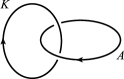
Figure 1. Hopf link $L$

Proof.

Note that the exterior of the Hopf link $(S^{3}\setminus\nu L)$ is diffeomorphic to $S^{1}\times\mathbb{A}$, where $\mathbb{A}\cong S^{1}\times[0,1]$ is an annulus. Hence there is a diffeomorphism between the cylinder $\partial(\nu F)\times[0,1]=T^{2}\times\partial D^{2}\times[0,1]$ and the Cartesian product $[S^{1}\times(S^{3}\setminus\nu L)]$. We can easily check that our link surgery gluing data is consistent with the fiber sum construction, and gives

$$L(\mathfrak{D})=[E(1)\setminus\nu F]\cup[\partial(\nu F)\times[0,1]\hskip 1.0pt]\cup[E(1)\setminus\nu F]\cong E(2).\qed$$

4. Two Symplectic Forms on the Cylinder $\partial(\nu F)\times[0,1]$

Let $M:=(S^{3}\setminus\nu L)$ denote the complement of the tubular neighborhood of a 2-component Hopf link $L$ in $S^{3}$. We saw that $M$ is diffeomorphic to a solid torus minus a thickened core, i.e. $M\cong S^{1}\times\mathbb{A}(r_{0},r_{1})$, where $\mathbb{A}(r_{0},r_{1})=\{z\in\mathbb{C}\>:\>r_{0}\leq|z|\leq r_{1}\}$. (In Figure 4 the core is represented by the darkened circle wherein you have no “pineapple”.) Let $(r,\theta)$ be the polar coordinates on the annulus $\mathbb{A}(r_{0},r_{1})$ with $-\pi<\theta\leq\pi$. Let $(y,r,\theta)$ be the coordinate system on $M=S^{1}\times\mathbb{A}(r_{0},r_{1})$, where $y$ denotes the angular coordinate on the $S^{1}$ factor ($-\pi<y\leq\pi$). For the sake of concreteness, let us assume from now on that $r_{1}=r_{0}+1$.

Now define a 4-manifold with boundary $Y:=S^{1}\times M\cong[\partial(\nu F)\times[0,1]\hskip 1.0pt]$, and let $x$ be the angular coordinate on the first $S^{1}$ factor ($-\pi<x\leq\pi$). To distinguish this $S^{1}$ factor with coordinate $x$ from the $S^{1}$ factor in $M$ with coordinate $y$, we will denote them by $S^{1}_{x}$ and $S^{1}_{y}$, respectively.

4.1. First Family of Tori

Our first symplectic form on $Y$ will be

(4.1) $$dx\wedge dy\,+\,rdr\wedge d\theta\,=\,\left.\omega_{f}\right|_{\partial(\nu F)\times[0,1]},$$

where $\omega_{f}$ is the symplectic form on $E(2)$ coming from the elliptic fibration $f$ (see Section 5). Now let $B$ be a $q$-strand braid whose closure $\hat{B}$ is a single-component link, i.e. a knot. It is not hard to embed $\hat{B}$ into the link exterior $M$ such that $S^{1}_{x}\times\hat{B}\subset Y$ is a symplectic submanifold with respect to the symplectic form (4.1). We choose a particular family of embeddings shown in Figure 2. Here we require the linking numbers to be $lk(\hat{B},K)=q\,$ and $lk(\hat{B},A)=m$.

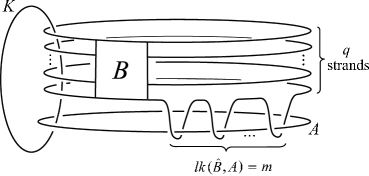
Figure 2. A family of embeddings of $\hat{B}$ into $(S^{3}\setminus\nu L)$

Let us denote this family of embeddings by $\phi_{q,m}:\hat{B}\rightarrow M$. Then we have the following.

Lemma 4.1.

For every pair of integers $q\geq 2$ and $m\geq 1$, the torus $S^{1}_{x}\times\phi_{q,m}(\hat{B})$ is a symplectic submanifold of $Y$ with respect to the symplectic form $(\ref{eq:symplectic form})$.

Proof.

We easily see that the restriction of the symplectic form (4.1) to $S^{1}_{x}\times\phi_{q,m}(\hat{B})$ is going to be just the restriction of $dx\wedge dy$, which does not vanish if we can arrange to have $dy\neq 0$ on the curve $\phi_{q,m}(\hat{B})$. But this is always possible since we can embed $\hat{B}$ in such a way that it is transverse to every annulus of the form, $\{{\rm point}\}\times\mathbb{A}(r_{0},r_{1})$, inside $M$. ∎

4.2. Second Family of Tori

Our second symplectic form on $Y$ will be

(4.2) $$\omega_{s}:=dx\wedge(dy+s\cdot d\theta)+rdr\wedge d\theta\,,$$

where $s>0$ is a sufficiently small real constant to be determined later (see Section 5). We easily check that $d\omega_{s}=0$, and

$$\omega_{s}\wedge\omega_{s}\,=\,2r\,dx\wedge dy\wedge dr\wedge d\theta\,\neq\,0\,.$$

Let $B$ be a $q$-strand braid as before. We describe an alternative way to embed the closure $\hat{B}$ into $M$. (See Figures 3 and 4.) Except for a single connected arc $I$, the closed braid $\hat{B}$ lies inside a thin “pineapple slice” of height $2\varepsilon$, $\{(y,r,\theta)\>:\>-\varepsilon\leq y\leq\varepsilon\}$. The remaining single arc $I$ traverses $m$ times around the solid torus (minus core) in the positive $y$-direction ($m\geq 1$). Away from the crossings and $I$, we require the circular arcs of $\hat{B}$ to lie on a fixed level annulus, $\mathbb{A}_{0}:=\{\,(y,r,\theta)\in M\>:\>y=0,\;r_{0}+\frac{1}{4}\leq r\leq r_{0}+\frac{3}{4}\,\}$. Note that the linking numbers are now $\,lk(\hat{B},K)=m\,$ and $\,lk(\hat{B},A)=q$. Essentially what we are doing differently this time is reversing the roles of $K$ and $A$ in our first family of embeddings $\phi_{q,m}$ above. (Compare Figures 2 and 8.)

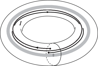
Figure 3. An embedding of $\hat{B}$ into $M$ with $m=2$

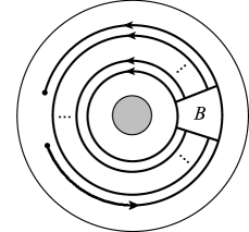
Figure 4. Bird’s eye view of the “pineapple slice”

Obviously, $S^{1}_{x}\times(S^{1}_{y}\times\{{\rm point}\})$ is a symplectic torus in $Y$ with respect to $\omega_{s}$. We show that $\hat{B}$ can be embedded into $M$ so that $S^{1}_{x}\times\hat{B}$ is also a symplectic torus in $(Y,\omega_{s})$. The crucial condition is that the restriction of the 1-form $\eta_{s}:=dy+s\cdot d\theta\in\Omega^{1}(M)$ has a fixed sign over the curve $\hat{B}$.

First orient the curve $\hat{B}$ as in Figures 3 and 4. Let $\gamma:[0,\ell]\rightarrow\hat{B}$ be a parametrization of $\hat{B}$ by arc-length. On the arc $I$, we may arrange to have

$$\langle dy,\dot{\gamma}\rangle\approx 1\,\quad{\rm and}\quad\langle d\theta,\dot{\gamma}\rangle\geq 0$$

as we traverse along the arc $I$ in the direction of the chosen orientation. This is possible because we can always embed $I$ so that $I$ is very close to being parallel to the (removed) core of the solid torus. Hence $\langle\eta_{s},\dot{\gamma}\rangle>0$, i.e. the 1-form $\eta_{s}$ is always positive on $I$ in the chosen direction.

Next note that $\langle d\theta,\dot{\gamma}\rangle=1$, and $\,\langle dr,\dot{\gamma}\rangle=\langle dy,\dot{\gamma}\rangle=0$, away from the crossings in $\mathbb{A}_{0}$. Hence the restriction of $\eta_{s}$ is positive on $\hat{B}\cap\mathbb{A}_{0}$, away from the crossings.

At a crossing in $B$, both $r$ and $y$ vary, so we need to draw the braid such that

(4.3) $$\left|\frac{dy}{d\theta}\right|\,=\,\left|\frac{dy/dt}{d\theta/dt}\right|\,<\,s\>.$$

Since we always have $\langle d\theta,\dot{\gamma}\rangle=d(\theta\circ\gamma)/dt=d\theta/dt>0$ at any crossing, an easy triangle inequality argument shows that $\langle\eta_{s},\dot{\gamma}\rangle>0$ at every crossing.

In other words, we need to embed the braid $B$ so that every pair of crossing arcs looks very short in terms of height $y$. More precisely, we need to ensure that, as we traverse along the crossing arcs in counter-clockwise direction, the angle $\theta$ is changing at a much faster rate than the rate of change for the height $y$.

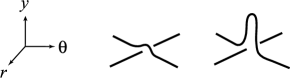
Figure 5. A “good” crossing and a “bad” crossing.

In Figure 5, the left crossing is short-looking and hence “good”, while the right crossing is something that we must avoid. To satisfy (4.3) for small values of $s$, we will have to embed the crossing arcs of $B$ very flat. However note that there is no limitation on the number of crossings or the number of strands allowed.

Finally we need to verify that $\eta_{s}$ is positive on the two “corners” (which are represented by the two black dots in Figures 3 and 4) where the arc $I$ is being attached to the rest of $\hat{B}$. Note that we can always assume that $r$ is constant on these two attaching portions of $\hat{B}$. We can easily smooth out the corners such that $\langle d\theta,\dot{\gamma}\rangle\geq 0$, $\langle dy,\dot{\gamma}\rangle\geq 0$, and the two quantities do not simultaneously vanish (see Figure 6). Hence the restriction of $dy+s\cdot d\theta$ to the two corners is strictly positive on the velocity vector $\dot{\gamma}$.

Figure 6. Smooth corners at $r={\rm constant}$

We conclude that $\eta_{s}$ restricts to some positive function multiple of the orientation 1-form on $\hat{B}$. Hence $\omega_{s}|_{p}=dx\wedge\eta_{s}|_{p}\neq 0$, for every point $p=(x,\gamma(t))\in S^{1}_{x}\times\hat{B}$. Let us denote this family of embeddings we constructed by $\psi_{q,m}:\hat{B}\rightarrow M$. In summary, we have the following.

Lemma 4.2.

$\omega_{s}$ is a symplectic form on $Y\!=\partial(\nu F)\times[0,1]$ with respect to which the torus $S^{1}_{x}\times\psi_{q,m}(\hat{B})$ is a symplectic submanifold for every pair of integers $q\geq 2$ and $m\geq 1$.

5. Two Families of Homologous Symplectic Tori in $E(2)$

Lemma 5.1.

There exists a symplectic $2$-form $\omega_{f}$ on $E(2)$, with respect to which the surfaces $F$ and $S$ are symplectic and $R_{1}$ and $R_{2}$ are Lagrangian submanifolds. By an arbitrarily small perturbation of $\omega_{f}$, we can obtain another symplectic form on $E(2)$ with respect to which $F,S$ are still symplectic and $R_{1}$ and/or $R_{2}$ are also symplectic.

Proof.

There is a symplectic form $\omega_{f}$ on $E(2)$ which is induced by the elliptic fibration $f\!:\!E(2)\rightarrow\mathbb{CP}^{1}$, essentially as the sum of symplectic forms in the fiber and the base (see [Th]). With respect to $\omega_{f}$ a regular fiber $F$ and section $S$ are symplectic, whereas the rim tori $R_{1}$ and $R_{2}$ are Lagrangian since the circles $C_{1}$ and $C_{2}$ lie in $F$ and $\partial D^{2}$ is embedded in a section. Since each $[R_{i}]$ is non-torsion and in fact $[R_{1}]$ and $[R_{2}]$ are linearly independent, as a consequence of the following more general lemma, we know that $\omega_{f}$ could be slightly perturbed in order to make $R_{1}$ and/or $R_{2}$ symplectic. ∎

Lemma 5.2 (cf. Lemma 1.6 in [Go]).

Let $X$ be a closed $4$-manifold with a symplectic form $\omega$ with respect to which closed, connected and disjoint submanifolds $\Sigma_{1},\Sigma_{2},\dots,\Sigma_{r}$ are Lagrangian. Suppose that the homology classes $[\Sigma_{1}],[\Sigma_{2}],\dots,[\Sigma_{r}]$ are non-torsion and linearly independent. Then there exists an arbitrarily small perturbation $\omega^{\prime}$ of $\omega$ which is symplectic and with respect to which all surfaces $\Sigma_{1},\Sigma_{2},\dots,\Sigma_{r}$ are symplectic submanifolds.

To prove the above lemma, one needs to choose a closed 2-form $\Omega$ on $X$ such that $\int_{\Sigma_{i}}\Omega>0\,$ for each $i$. Then $\omega^{\prime}:=\omega^{\prime}_{s}:=\omega+s\Omega\,$ is a suitable perturbation for sufficiently small constant $s>0$.

Theorem 5.3.

Fix a pair of integers $q\geq 2$ and $m\geq 1$.
(i) The embedded torus $S^{1}_{x}\times\phi_{q,m}(\hat{B})\subset E(2)$ is a symplectic submanifold with respect to the symplectic form $\omega_{f}$, and represents the homology class $q[F]+m[R_{1}]$.
(ii) The embedded torus $S^{1}_{x}\times\psi_{q,m}(\hat{B})\subset E(2)$ represents $m[F]+q[R_{1}]$, and there is a symplectic form on $E(2)$ with respect to which this torus is a symplectic submanifold.

Proof.

(i) Without loss of generality, we may assume that the restriction of $\omega_{f}$ to the subset $Y=\partial(\nu F)\times[0,1]$ is given by (4.1). This immediately implies that $S^{1}_{x}\times\phi_{q,m}(\hat{B})$ embeds symplectically into $E(2)$. The link surgery gluing data $\mathfrak{D}$ in (3.1) of Lemma 3.2 directly gives the homology class of $S^{1}_{x}\times\phi_{q,m}(\hat{B})$ in $E(2)$ since we have $[\phi_{q,m}(\hat{B})]=q[\mu(K)]+m[\lambda(K)]\in H_{1}(S^{3}\setminus\nu L;\mathbb{Z})$, and $S^{1}_{x}$ gets identified with $C_{1}$.

(ii) In Section 4, we have already shown that the torus $S^{1}_{x}\times\psi_{q,m}(\hat{B})$ is a symplectic submanifold of $Y=\partial(\nu F)\times[0,1]\hskip 1.0pt$ with respect to the symplectic form $\omega_{s}$ for any $s>0$. By definition (4.2), $\omega_{s}=dx\wedge dy+rdr\wedge d\theta+s\cdot dx\wedge d\theta$ near the boundary of $Y$. Choosing the perturbation (which makes only $R_{1}$ symplectic) in Lemma 5.1 carefully (e.g. $\Omega=dx\wedge d\theta$ with respect to the local coordinates in which $\omega_{f}=dx\wedge dy+rdr\wedge d\theta$) we could make sure that there exists a symplectic form $\omega^{\prime}$ on

$$E(2)\;\cong\;[E(1)\setminus\nu F]\cup[\partial(\nu F)\times[0,1]\hskip 1.0pt]\cup[E(1)\setminus\nu F]$$

which restricts (up to isotopy) to $dx\wedge dy+rdr\wedge d\theta+s\cdot dx\wedge d\theta$ near the boundary $\partial[\partial(\nu F)\times[0,1]\hskip 1.0pt]$. This allows us to extend $\omega_{s}$ to the closed manifold $E(2)$.

The link surgery gluing data $\mathfrak{D}$ in (3.1) again gives the homology class of $S^{1}_{x}\times\psi_{q,m}(\hat{B})$ in $E(2)$ since we have $[\psi_{q,m}(\hat{B})]=m[\mu(K)]+q[\lambda(K)]$ this time around. ∎

Remark 5.4.

Recall that we chose the factorization $F=C_{1}\times C_{2}$ in the link surgery gluing data $\mathfrak{D}$ in (3.1) of Lemma 3.2. If instead we had chosen the (reverse order) identification $F=C_{2}\times C_{1}$, then the tori $S^{1}_{x}\times\phi_{q,m}(\hat{B})$ and $S^{1}_{x}\times\psi_{q,m}(\hat{B})$ would have represented the homology classes $q[F]+m[R_{2}]\,$ and $m[F]+q[R_{2}]\,$ in $H_{2}(E(2);\mathbb{Z})$, respectively.

6. Alexander Polynomials Corresponding to Particular Braids

In order to distinguish the isotopy classes of the homologous symplectic tori we constructed in the previous section, we will compute the Seiberg-Witten invariants of 4-manifolds that are obtained as the fiber sum of $E(2)$ along these tori and the rational elliptic surface $E(1)$ along one of its regular fibers. We will see that the Seiberg-Witten invariant of such a 4-manifold is essentially the Alexander polynomial of the 3-component link obtained from the braid $B$ as seen in Figures 7 and 8. Both figures are for the embedded tori $S^{1}_{x}\times\psi_{q,m}(\hat{B})$, and the corresponding pictures for $S^{1}_{x}\times\phi_{q,m}(\hat{B})$ are obtained by simply relabelling the $K$ component $A$ and vice versa.

In this section we will present the “simplest” family of braids that is most amenable to the computation of the Alexander polynomials of the corresponding links. A generic member $B=B_{k,q}$ of this family is shown in Figure 9 as the upper left part (inside the dotted rectangle) of the braid $B(q;k,m)$, for which the desired 3-component link $L\cup\psi_{q,m}(\hat{B})$ is $A\cup\hat{B}(q;k,m)$, where $A$ is the axis of the closed braid $\hat{B}(q;k,m)$ as well as one of the components of the Hopf link $L=K\cup A$.

Similarly, we have $L\cup\phi_{q,m}(\hat{B})=K\cup\hat{B}(q;k,m)$, where $K$ now denotes the axis of the braid $B(q;k,m)$ and $A$ is the bottom strand in Figure 9.

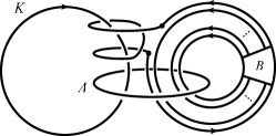
Figure 7. 3-component link $L\cup\psi_{q,m}(\hat{B})$ with $m=2$

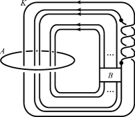
Figure 8. 3-component link $L\cup\psi_{q,m}(\hat{B})$ with $m=2$ in braid form

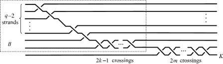
Figure 9. $(q+1)$-strand braid $B(q;k,m)$ with $k,m\geq 1$, $q\geq 2$

Remark 6.1.

Note that we are using the same family of braids $B$ as in [EP1]. Consequently, when $m=0$ and $q\geq 2$, we obtain families of tori representing either $q[F]$ or $q[R_{i}]$ that we already constructed in [EP1].

Lemma 6.2.

Let $\Delta_{q;k,m}(x,s,t)$ denote the Alexander polynomial of the three-component link $L\cup\psi_{q,m}(\hat{B})=A\cup\hat{B}(q;k,m)\hskip 1.0pt$, where the variables $x$, $s$ and $t$ correspond to the axis $A$, unknot $K$ and the closed braid $\hat{B}$ respectively. Then $\Delta_{q;k,m}(x,s,t)=$

$$1-x(st)^{m}+x\cdot\frac{(xt)^{q-1}-1}{xt-1}\left[t^{2k-1}+t(s-1)\,\frac{t^{2k-1}+1}{t+1}\cdot\frac{(st)^{m}-1}{st-1}-x(st)^{m}t^{2k-1}\right].$$

The Alexander polynomial of the link $L\cup\phi_{q,m}(\hat{B})=K\cup\hat{B}(q;k,m)\hskip 1.0pt$ is given by $\Delta_{q;k,m}(s,x,t)$, i.e. the polynomial obtained from $\Delta_{q;k,m}(x,s,t)$ by switching the variables $x$ and $s$.

Proof.

The braid group on $q$ strands is generated by the elementary braid transpositions $\sigma_{1},\dots,\sigma_{q-1}\hskip 1.0pt$, where $\sigma_{i}$ denotes the crossing of the ( $i$ +1)st strand over the $i$-th. Note that

$$B(q;k,m)\,=\>\sigma_{q}\,\sigma_{q-1}\,\cdots\,\sigma_{3}\,\sigma_{2}^{2k-1}\,\sigma_{1}^{2m}\,.$$

By Theorem 1 in [Mo], we have

(6.1) $$\Delta_{q;k,m}\,:=\,\Delta_{q;k,m}(x,s,t)\,=$$

$$\det\left(I-x\,C^{(q)}_{q}(t)C^{(q)}_{q-1}(t)\cdots\,C^{(q)}_{3}(t)[C^{(q)}_{2}(t)]^{2k-1}[C^{(q)}_{1}(s)C^{(q)}_{1}(t)]^{m}\right)\,,$$

where $C^{(q)}_{i}(a)$ denotes the following $q\times q$ matrix which differs from the identity matrix $I$ only in the three places shown on the $i$-th row.

$$C^{(q)}_{i}(a)\;:=\;\left(\begin{array}[]{ccccccc}1&&&&&&\\ &\ddots&&&&&\\ &&1&&&&\\ &&a&-a&1&&\\ &&&&1&&\\ &&&&&\ddots&\\ &&&&&&1\end{array}\right)\!\!\begin{array}[]{r}\\ \\ \\ \\ \\ \\ \\ .\\ \end{array}$$

When $i=1$ or $i=q\hskip 1.0pt$, the matrix is truncated appropriately to give two non-zero entries in row $i$.

The main step of this proof is showing that $D_{q;k,m}=xtD_{q-1;k,m}$ for all $q\geq 2$, where $D_{q;k,m}:=\Delta_{q+1;k,m}-\Delta_{q;k,m}$ and $\Delta_{1;k,m}:=1-x(st)^{m}$. During this process we get

$$\Delta_{2;k,m}\!\!\! = \!1-x^{2}(st)^{m}t^{2k-1}$$

$$+ \!\!x\left[t^{2k-1}-(st)^{m}+(s-1)t\left(\frac{t^{2k-1}+1}{t+1}\right)\left(\frac{(st)^{m}-1}{st-1}\right)\right]\,.$$

This calculation leads to

$$D_{1;k,m}=x\left[t^{2k-1}+(s-1)t\left(\frac{t^{2k-1}+1}{t+1}\right)\left(\frac{(st)^{m}-1}{st-1}\right)\right]-x^{2}(st)^{m}t^{2k-1}$$

and hence $D_{q;k,m}=$

$$(xt)^{q-1}\left\{x\left[t^{2k-1}+(s-1)t\left(\frac{t^{2k-1}+1}{t+1}\right)\left(\frac{(st)^{m}-1}{st-1}\right)\right]-x^{2}(st)^{m}t^{2k-1}\right\}.$$

By putting the pieces together we finish the proof of the lemma.

By Equation (6.1) $\Delta_{q+1;k,m}=\det(I-x\Gamma_{q+1;k,m})$, where

$$\Gamma_{q+1;k,m}=C^{(q+1)}_{q+1}(t)C^{(q+1)}_{q}(t)\cdots\,C^{(q+1)}_{3}(t)\!\!\left[C^{(q+1)}_{2}(t)\right]^{2k-1}\left[C^{(q+1)}_{1}(s)C^{(q+1)}_{1}(t)\right]^{m}.$$

Note that

$$C^{(q+1)}_{i}(t)\;=\;\left(\begin{array}[]{cccc}&&&0\\ &C^{(q)}_{i}(t)&&\vdots\\ &&&0\\ 0&\dots&0&1\end{array}\right)$$

for $i\in\{1,2,\dots,q-1\},\;$ so we must have $\Gamma_{q+1;k,m}=$

$$= C^{(q+1)}_{q+1}(t)C^{(q+1)}_{q}(t)\left(\begin{array}[]{cccc}&&&0\\ &C^{(q)}_{q}(t)&&\vdots\\ &&&0\\ 0&\dots&0&1\end{array}\right)^{\begin{array}[]{l}-1\end{array}}\left(\begin{array}[]{cccc}&&&0\\ &\Gamma_{q;k,m}&&\vdots\\ &&&0\\ 0&\dots&0&1\end{array}\right)$$

$$= \left(\begin{array}[]{cccc}1&&&\\ &\ddots&&\\ &&1&1\\ &&t&0\end{array}\right)\left(\begin{array}[]{cccc}&&&0\\ &\Gamma_{q;k,m}&&\vdots\\ &&&0\\ 0&\dots&0&1\end{array}\right)\!\!\begin{array}[]{r}\\ \\ \\ .\end{array}$$

Hence it follows that

(6.5) $$\Gamma_{q+1;k,m}\;=\;\left(\begin{array}[]{cc}&0\\ \Gamma_{q;k,m}&\vdots\\ &0\\ &1\\ t\,(\Gamma_{q;k,m})_{(q\hskip 1.0pt,\,\ast\hskip 1.0pt)}&0\end{array}\right)$$

and

(6.6) $$\;I-x\Gamma_{q+1;k,m}\>=\>\left(\begin{array}[]{cc}&0\\ I-x\Gamma_{q;k,m}&\vdots\\ &0\\ &-x\\ -xt\,(\Gamma_{q;k,m})_{(q\hskip 1.0pt,\,\ast\hskip 1.0pt)}&1\end{array}\right)\!\!\begin{array}[]{r}\\ \\ \\ \\ ,\end{array}$$

where $(\Gamma_{q;k,m})_{(q\hskip 1.0pt,\,\ast\hskip 1.0pt)}$ denotes the last row of $\Gamma_{q;k,m}\hskip 1.0pt$. When we calculate the determinant of the matrix $I-x\Gamma_{q+1;k,m}$ by expanding along its last column we get the following equality:

(6.7) $$\;\det(I-x\Gamma_{q+1;k,m})\;=$$

$$\det(I-x\Gamma_{q;k,m})-(-x)t\left[\det(I-x\Gamma_{q;k,m})-\det(I-x\Gamma_{q-1;k,m})\right]\,.$$

To prove the above equality for $q\geq 3$, observe that, in this case, all but the last row of the minor of the matrix $I-x\Gamma_{q+1;k,m}$ corresponding to the entry $-x$ in the last column are the same as the rows of $I-x\Gamma_{q;k,m}\hskip 1.0pt$, and the last row of the minor is $t$ times the last row of $I-x\Gamma_{q;k,m}$ except for the last entry. In the minor, this entry is $0$, whereas in $I-x\Gamma_{q;k,m}\hskip 1.0pt$ this entry is $1$ (since Equation (6.5) shows that the last diagonal entry of $\Gamma_{q;k,m}$ is $0$ as long as $q\geq 3$). This observation is why the determinant of the minor corresponding to $-x$ is $t$ times the difference between the determinant of $I-x\Gamma_{q;k,m}$ and the determinant of the minor of $I-x\Gamma_{q;k,m}$ obtained by deleting the last row and the last column (and this minor is nothing but $I-x\Gamma_{q-1;k,m}$).

For $q=2$, Equation (6.7) is proved by direct calculation of $\Delta_{2;k,m}$ and $\Delta_{3;k,m}$. Note that we defined $\Delta_{1;k,m}$ to be $1-x(st)^{m}$. In fact, once $I-x\Gamma_{2;k,m}$ is verified to be

$$\left(\!\!\begin{array}[]{cc}1-x(st)^{m}&x(s-1)\frac{(st)^{m}-1}{st-1}\\[7.0pt] -xt(st)^{m}\frac{t^{2k-1}+1}{t+1}&\;\;1+x(s-1)t\frac{t^{2k-1}+1}{t+1}\frac{(st)^{m}-1}{st-1}+xt^{2k-1}\end{array}\!\!\right)$$

with the help of the equalities

$$\left(\begin{array}[]{cc}1&0\\ t&-t\end{array}\right)^{2k-1}=\;\left(\!\begin{array}[]{cc}1&0\\ t\cdot\frac{t^{2k-1}+1}{t+1}&-t^{2k-1}\end{array}\!\right)$$

and

$$\left(\!\begin{array}[]{cc}st&-s+1\\ 0&1\end{array}\!\right)^{m}=\;\left(\!\!\begin{array}[]{cc}(st)^{m}&-(s-1)\frac{(st)^{m}-1}{st-1}\\ 0&1\end{array}\!\!\right),$$

one not only gets Equation (6) regarding $\Delta_{2;k,m}$, but also the matrix $I-x\Gamma_{3;k,m}$ by using Equation (6.6). As a result of expanding the $3\times 3$ matrix $I-x\Gamma_{3;k,m}$ along its last column, it is easily seen that

$$\Delta_{3;k,m}=\>\Delta_{2;k,m}+x\{t[\Delta_{2;k,m}-(1-x(st)^{m})]\}\,.$$

Equation (6.7) and the calculations above give

$$D_{q;k,m}\!\!\! = \!\!\!xtD_{q-1;k,m}$$

$$= \!\!\!(xt)^{q-1}x\left[t^{2k-1}+(s-1)t\,\frac{t^{2k-1}+1}{t+1}\cdot\frac{(st)^{m}-1}{st-1}-x(st)^{m}t^{2k-1}\right]\,.$$

Finally, the formula in the statement of the lemma is a consequence of

$$\Delta_{q;k,m}\,=\>\Delta_{1;k,m}+D_{1;k,m}+\cdots+D_{q-1;k,m}$$

$$\hskip 35.56593pt=\>1-x(st)^{m}+\,\frac{(xt)^{q-1}-1}{xt-1}\,D_{1;k,m}\>.\qed$$

Corollary 6.3.

The number of nonzero terms in the polynomial $\Delta_{q;k,m}(x,s,t)$ is equal to $[6-4q]+k[2(m+1)(q-1)]$.

Proof.

The polynomial $\Delta_{q;k,m}$ could be written as

$$\Delta_{q;k,m} = 1+x\{-(st)^{m}+P_{k,m}(s,t)\}$$

$$+\>x^{2}\{t[-(st)^{m}t^{2k-2}+P_{k,m}(s,t)]\}$$

$$+\>\cdots$$

$$+\>x^{q-1}\{t^{q-2}[-(st)^{m}t^{2k-2}+P_{k,m}(s,t)]\}$$

$$+\>x^{q}\{-(st)^{m}t^{2k+q-3}\}\>,$$

where

$$P_{k,m}(s,t)=t^{2k-1}+(s-1)t\,\frac{(st)^{m}-1}{st-1}\cdot\frac{t^{2k-1}+1}{t+1}\ .$$

A direct count of nonzero terms in $P_{k,m}(s,t)$ gives $2km+2k-3$, and as a consequence, for $0<i<q$, the number of nonzero terms in $\Delta_{q;k,m}$ that are divisible by $x^{i}$ but not divisible by $x^{i+1}$ is $2km+2k-4$. The formula is then easily obtained as a result of an effort to write the desired expression in a form that emphasizes the dependence of the count on $k$ when $m$ and $q$ are fixed. ∎

7. Non-Isotopy: Seiberg-Witten Invariants

In Section 5, for each $i\in\{1,2\}$, $m\geq 1$ and $q\geq 2$ we explained the construction of a symplectic torus representing $q[F]+m[R_{i}]$ or $m[F]+q[R_{i}]$ using a suitable $q$-component braid $B$. Let $\jmath$ denote either $\phi_{q,m}$ or $\psi_{q,m}$. The 4-manifold $E(2)\#_{T=F}E(1)$, obtained as the fiber sum of $E(1)$ along a regular fiber $F$ with $E(2)$ along one of these tori $T\!:=S^{1}_{x}\times\jmath(\hat{B})$ we constructed, is easily seen to be diffeomorphic to the link surgery manifold $(L\cup\jmath(\hat{B}))(\mathfrak{D}^{\prime})$, where $\mathfrak{D}^{\prime}$ is the link surgery gluing data

$$\left(\{(\mu(K),\lambda(K)),(\lambda(A),-\mu(A)),(\lambda(\jmath(\hat{B})),-\mu(\jmath(\hat{B})))\},\{E(1),F=C_{1}\times C_{2}\}_{i=1}^{3}\right).$$

In Section 6, we looked at a particular family of braids $B=B_{k,q}$ for which

$$L_{\jmath}\,:=\,L\cup\jmath(\hat{B})\;=\left\{\!\!\begin{array}[]{lcl}K\cup\hat{B}(q;k,m)&{\rm if}&\jmath=\phi_{q,m}\,,\\[5.0pt] A\cup\hat{B}(q;k,m)&{\rm if}&\jmath=\psi_{q,m}\,.\end{array}\right.$$

In this section, we will distinguish the symplectic tori that come from this family of braids by comparing the Seiberg-Witten invariants of $L_{\jmath}(\mathfrak{D}^{\prime})$.

Recall that the Seiberg-Witten invariant $\overline{SW}_{\!\!X}$ of a 4-manifold $X$ (satisfying $b_{2}^{+}(X)>1$) can be thought of as an element of the group ring of $H_{2}(X;\mathbb{Z})$, i.e. $\overline{SW}_{\!\!X}\in\mathbb{Z}[H_{2}(X;\mathbb{Z})]$. If we write $\overline{SW}_{\!\!X}=\sum_{g}a_{g}g\hskip 1.0pt$, then we say that $g\in H_{2}(X;\mathbb{Z})$ is a Seiberg-Witten basic class of $X$ if $a_{g}\neq 0$. Since the Seiberg-Witten invariant of a 4-manifold is a diffeomorphism invariant, so is the total number of Seiberg-Witten basic classes.

Regarding the Seiberg-Witten invariants of $L_{\jmath}(\mathfrak{D}^{\prime})$, we have the following lemma which is an easy consequence of the gluing formulas for the Seiberg-Witten invariant in [FS1], [Pa] and [Ta]. Detailed arguments can be found in [EP1], [MT] or [V1].

Lemma 7.1.

Let $\iota:[S^{1}\times(S^{3}\setminus\nu L_{\jmath})]\rightarrow L_{\jmath}(\mathfrak{D}^{\prime})$ be the inclusion map. Let $\xi:=\iota_{\ast}[S^{1}\times\mu(A)],$ $\tau:=\iota_{\ast}[S^{1}\times\mu(K)],$ $\zeta:=\iota_{\ast}[S^{1}\times\mu(\jmath(\hat{B}))]\in H_{2}(L_{\jmath}(\mathfrak{D}^{\prime});\mathbb{Z}).$ Then the Seiberg-Witten invariant of $L_{\jmath}(\mathfrak{D}^{\prime})$ is

$$\overline{SW}_{\!L_{\jmath}(\mathfrak{D}^{\prime})}\!\! = \!\!\Delta^{{\rm sym}}_{L_{\jmath}}(\xi^{2},\tau^{2},\zeta^{2})$$

$$= \!\!\left\{\!\!\begin{array}[]{ccc}\tau^{-q}\xi^{-m}\zeta^{-(2k+q+m-3)}\Delta_{q;k,m}(\tau^{2},\xi^{2},\zeta^{2})&{\rm if}&\jmath=\phi_{q,m}\,,\\[9.0pt] \xi^{-q}\tau^{-m}\zeta^{-(2k+q+m-3)}\Delta_{q;k,m}(\xi^{2},\tau^{2},\zeta^{2})&{\rm if}&\jmath=\psi_{q,m}\,,\end{array}\right.$$

where $\Delta_{q;k,m}$ is the Alexander polynomial in Lemma 6.2, and $\Delta^{{\rm sym}}$ stands for the symmetrized Alexander polynomial.

Note that $\xi,\tau$ and $\zeta$ are linearly independent in $H_{2}(L_{\jmath}(\mathfrak{D}^{\prime});\mathbb{Z})$ as in Proposition 3.2 of [MT]. As a consequence of Corollary 6.3, the number of Seiberg-Witten basic classes of $L_{\jmath}(\mathfrak{D}^{\prime})$ depends on $k$ for fixed $q\geq 2$ and $m\geq 1$. Hence, for fixed triple $q$, $m$ and $\jmath\hskip 1.0pt$, the family of 4-manifolds $\{L_{\jmath}(\mathfrak{D}^{\prime})\}_{k\geq 1}$ are all pairwise non-diffeomorphic. On the other hand, the diffeomorphism type of $L_{\jmath}(\mathfrak{D}^{\prime})\cong E(2)\#_{T=F}E(1)$ only depends on the isotopy type of $T$.

This finishes the proof of Theorem 2.1. In fact, one can easily see that the tori we constructed are different even under self-diffeomorphisms of $E(2)$.

8. Generalization to Other Symplectic 4-Manifolds

For certain elliptic surfaces, our result easily generalizes. Since our tori will remain non-isotopic even after fiber sum and link surgery (cf. [FS4]), we immediately obtain the analogue of Theorem 2.1 for the fiber sums $E(n)=E(2)\#_{F}E(n-2)$ for $n\geq 3$, and the knot surgery manifolds

$$E(n)_{K}:=\>K(\{(\alpha_{1},\beta_{1})=(\mu(K),\lambda(K))\},\{E(n),F=C_{1}\times C_{2}\})$$

for any fibred knot $K\subset S^{3}$ and $n\geq 2$. (Note that the knot $K$ needs to be fibred to ensure that $E(n)_{K}$ is symplectic, and $E(n)_{K}$ can also be viewed as the fiber sum $E(n-1)\#_{F}E(1)_{K}\hskip 1.0pt$.) Also note that an infinite subset of our homologous symplectic tori will continue to remain different under self-diffeomorphisms of these symplectic 4-manifolds, since the number of Seiberg-Witten basic classes of the corresponding link surgery manifolds always goes to infinity as $k\rightarrow\infty$ and $q,m$ are fixed.

In particular, we recover and generalize Vidussi’s result (Corollary 1.2 in [V3]) on the non-isotopic symplectic representatives of primitive homology classes on certain knot surgery manifolds $E(2)_{K}$ (also see [FS3]).

For more general symplectic 4-manifolds, note that the Hopf link will give us any fiber sum manifold like $E(2)$. More precisely, if $Z$ is obtained as the symplectic fiber sum along symplectic tori of self-intersection $0$, then by choosing a suitable link surgery gluing data, we can symplectically embed $S^{1}_{x}\times\jmath(\hat{B})$ in $Z$. In order to distinguish these tori we can still use Seiberg-Witten theory, but we need some extra assumptions to make use of the gluing formulas for the Seiberg-Witten invariant.

Theorem 8.1.

Suppose that $F_{i}$ is a symplectically embedded $2$-torus in a closed symplectic $4$-manifold $Z_{i}$ with $b^{+}_{2}(Z_{i})>1$, $[F_{i}]^{2}=0$ and $H^{1}(Z_{i}\setminus\nu F_{i};\mathbb{Z})=0$, for each $i\in\{1,2\}$. Let $Z=Z_{1}\#_{F_{1}=F_{2}}Z_{2}$ be the symplectic fiber sum of $Z_{1}$ and $Z_{2}$ along $F_{1}$ and $F_{2}$. Let $[F]$ and $[R]$ be the homology classes of $F_{1}=F_{2}$ and a rim torus in $Z$, respectively. Then for any pair of positive integers $(q,m)\neq(1,1)$ there exists an infinite family of pairwise non-isotopic symplectic tori representing the homology class $q[F]+m[R]\in H_{2}(Z;\mathbb{Z})$.

Proof.

Let $L$ denote a Hopf link in $S^{3}$ as before. We can express $Z=L(\mathfrak{D}^{\prime\prime})$, where

$$\mathfrak{D}^{\prime\prime}:=\>\big{(}\{(\mu(K),\lambda(K)),(\lambda(A),-\mu(A))\},\{Z_{i},F_{i}=C^{i}_{1}\times C^{i}_{2}\}_{i=1}^{2}\big{)}\,.$$

The rim torus $R$ in the lemma is given by the Cartesian product $C^{i}_{1}\times\partial D^{2}$, where $D^{2}$ is a normal disk in $\nu F_{i}\cong F_{i}\times D^{2}$. We need to compute the Seiberg-Witten invariants of the corresponding link surgery manifolds $L_{\jmath}(\mathfrak{D}^{\prime\prime\prime})$, where

$$\mathfrak{D}^{\prime\prime\prime}\!\!\! := \!\!\!\big{(}\{(\mu(K),\lambda(K)),(\lambda(A),-\mu(A)),(\lambda(\jmath(\hat{B})),-\mu(\jmath(\hat{B})))\},$$

$$\{Z_{i},F_{i}=C^{i}_{1}\times C^{i}_{2}\}_{i=1}^{2}\cup\{E(1),F=C_{1}\times C_{2}\}\big{)}\,.$$

Just as in [EP1], the assumption that $H^{1}(Z_{i}\setminus\nu F_{i};\mathbb{Z})=0$ ($i=1,2$) is crucial. It allows us to conclude that the homology classes $[F]$ and $[R]$ are linearly independent in $H_{2}(Z;\mathbb{Z})$ as in Proposition 3.2 of [MT]. It also implies that the relative Seiberg-Witten invariants are

$$\overline{SW}_{\!Z_{i}\setminus\nu F_{i}}=\>([F_{i}]^{-1}-[F_{i}])\cdot\overline{SW}_{\!Z_{i}}\>\neq 0\,$$

by Corollary 20 in [Pa]. Hence the Seiberg-Witten invariants of $L_{\jmath}(\mathfrak{D}^{\prime\prime\prime})$ can be computed using the standard gluing formulas as before. The rest of the proof is the same as the proof of Theorem 2.1. Once again, to conclude that there are infinitely many tori that remain different under self-diffeomorphisms of $Z$, we observe that, for fixed pair $q$ and $m$, the number of Seiberg-Witten basic classes of $L_{\jmath}(\mathfrak{D}^{\prime\prime\prime})$ goes to infinity as $k\rightarrow\infty$. Non-isotopy is more simply obtained from a homology basis argument due to Fintushel and Stern (cf. [FS4]). ∎

Remark 8.2.

The conclusion of Theorem 8.1 may still apply even when $b_{2}^{+}(Z_{i})=1$. In that case, one must take care and define $\overline{SW}_{\!\!Z_{i}}:=\overline{SW}_{\!\!Z_{i},F_{i}}^{\hskip 1.0pt\pm}$ (see [FS1] and [Pa]). In general, for a closed 4-manifold $X$ with $b_{2}^{+}(X)=1$, it is not automatic that $\overline{SW}_{\!\!X}$ is a finite sum and $\overline{SW}_{\!\!X}\neq 0$ for a symplectic $X$. If indeed $\overline{SW}_{\!\!Z_{i}}\neq 0$ and is a finite sum, then Theorem 8.1 will still be valid for such $Z$. However if $\overline{SW}_{\!\!Z_{i}}=0$ or is an infinite sum, then there seems to be no systematic method currently available to check whether the tori in our family are mutually non-isotopic in $Z$ or not. An ad hoc method for a particularly simple infinite sum case is presented in [EP2] for a slightly different family of tori (corresponding to embeddings $\phi_{1,m}$).

Acknowledgments

We would like to thank Ronald Fintushel, Ian Hambleton, Maung Min-Oo, Sašo Strle and Stefano Vidussi for their encouragement and helpful comments. The figures were produced by the second author using Adobe^® Illustrator$\hskip 1.0pt{}^{\circledR}$ Version 10. Some computations in Section 6 were verified with the aid of Maple$\hskip 1.0pt{}^{\circledR}$ Version 8.

References

- [ADK] D. Auroux, S.K. Donaldson and L. Katzarkov: Luttinger surgery along Lagrangian tori and non-isotopy for singular symplectic plane curves, Math. Ann. 326 (2003), 185–203.
- [EP1] T. Etgü and B.D. Park: Non-isotopic symplectic tori in the same homology class, preprint. Available at arXiv:math.GT/0212356.
- [EP2] T. Etgü and B.D. Park: Homologous non-isotopic symplectic tori in homotopy rational elliptic surfaces, preprint. Available at arXiv:math.GT/0307029.
- [EP3] T. Etgü and B.D. Park: Homologous non-isotopic Lagrangian tori in symplectic 4-manifolds, in preparation.
- [FS1] R. Fintushel and R.J. Stern: Knots, links and -manifolds, Invent. Math. 134 (1998), 363–400.
- [FS2] R. Fintushel and R.J. Stern: Symplectic surfaces in a fixed homology class, J. Differential Geom. 52 (1999), 203–222.
- [FS3] R. Fintushel and R.J. Stern: Invariants for Lagrangian tori, preprint. Available at arXiv:math.SG/0304402.
- [FS4] R. Fintushel and R.J. Stern: Tori in symplectic -manifolds, preprint.
- [Go] R.E. Gompf: A new construction of symplectic manifolds, Ann. of Math. 142 (1995), 527–595.
- [GS] R.E. Gompf and A.I. Stipsicz: -Manifolds and Kirby Calculus, Graduate Studies in Mathematics 20, Amer. Math. Soc., 1999.
- [MT] C.T. McMullen and C.H. Taubes: -manifolds with inequivalent symplectic forms and -manifolds with inequivalent fibrations, Math. Res. Lett. 6 (1999), 681–696.
- [Mo] H.R. Morton: The multivariable Alexander polynomial for a closed braid, in Low-dimensional Topology, ed. Hanna Nencka, Contemporary Mathematics 233, Amer. Math. Soc. (1999), 167–172. Also available at arXiv:math.GT/9803138.
- [Pa] B.D. Park: A gluing formula for the Seiberg-Witten invariant along , Michigan Math. J. 50 (2002), 593–611.
- [Ta] C.H. Taubes: The Seiberg-Witten invariants and -manifolds with essential tori, Geom. Topol. 5 (2001), 441–519.
- [Th] W.P. Thurston: Some simple examples of symplectic manifolds, Proc. Amer. Math. Soc. 55 (1976), 467–468.
- [V1] S. Vidussi: Smooth structure of some symplectic surfaces, Michigan Math. J. 49 (2001), 325–330.
- [V2] S. Vidussi: Nonisotopic symplectic tori in the fiber class of elliptic surfaces, preprint. Available at http://www.math.ksu.edu/~vidussi/
- [V3] S. Vidussi: Lagrangian surfaces in a fixed homology class: Existence of knotted Lagrangian tori, preprint. Available at http://www.math.ksu.edu/~vidussi/
-
[V4]
S. Vidussi:
Symplectic tori in homotopy ’s, preprint. Available
at
http://www.math.ksu.edu/~vidussi/