Uniform 1-cochains and Genuine Laminations

Abstract.

We construct a pair of transverse genuine laminations on an atoroidal 3-manifold admitting transversely orientable uniform 1-cochain. The laminations are induced by the uniform 1-cochain and they are indeed the ”straightening” of the coarse laminations defined in [Ca], by using minimal surface techniques. Moreover, when you collapse these laminations, you can get a topological pseudo-Anosov flow, as defined by Mosher, [Mo].

1. Introduction

In [Ca], Calegari proved that if an atoroidal 3-manifold admits a uniform 1-cochain, then its fundamental group is Gromov-hyperbolic, and it has a coarse pseudo-Anosov package, which is defined below. These uniform 1-cochains are in some sense a generalization of slitherings, which are studied by Thurston in [Th].

The idea to get the laminations is indeed simple. By [Ca], if M admits a uniform 1-cochain, M is a Gromov hyperbolic manifold and we have coarse pseudo-Anosov package, so there is a coarse lamination in universal cover of the manifold, $\tilde{M}$. Using the asymptotic circles of this coarse lamination, we get a group-invariant family of circles, and using the minimal surface lemmas of Gabai in [Ga], we can span these circles with laminations by least area planes. Here we need least area planes to get $\pi_{1}$ equivariance in universal cover. Then all we need to show is that this union of laminations in universal cover can be modified to get a lamination in downstairs, in the original manifold.

1.1. Definitions:

The following definitions are from [Ca].

Definition 1.1.

Uniform 1-cochain on a 3-manifold M is a function $s:\pi_{1}(M){\rightarrow}\mathbf{R}$ satisfying

• $s(\alpha\beta)=s(\beta\alpha)$ for all $\alpha,\beta\in\pi_{1}(M)$

• $s(\alpha^{n})=ns(\alpha)$ for any $\alpha\in\pi_{1}(M)$ and $n\in Z$

• $|(\delta s)(\alpha,\beta)|=|s(\alpha)+s(\beta)-s(\alpha\beta)|\leq C_{M}$, where $C_{M}$ is a uniform constant only depends on M.

• For some $t$ the set

  $$L_{t}=\{\alpha\in\pi_{1}(M)\mid|s(\alpha)|\leq t\}$$

  is coarsely connected and coarsely simply connected as a metric space, with the metric inherited as a subspace of Cayley($\pi_{1}(M)$) with some word metric.

Here, coarsely connected intuitively means that when you realize $\pi_{1}(M)$ as a subset of universal cover of M, $\tilde{M}$ (like orbit of a point under deck transformations), it has an $\epsilon$ neighborhood which is connected, and similarly coarsely simply connected means that it has an $\epsilon$ neighborhood which is simply connected in $\tilde{M}$.

Definition 1.2.

A coarse pseudo-Anosov package for M is the following structure:

1. A pair of very full geodesic laminations $\lambda^{\pm}$ of ${\mathbf{H}}^{2}$ which are transverse to each other and bind ${\mathbf{H}}^{2}$ with transverse measures $\mu^{\pm}$ without atoms.

2. An automorphism $Z:{\mathbf{H}}^{2}{\rightarrow}{\mathbf{H}}^{2}$ which preserves $\lambda^{\pm}$ and multiplies the measures by k, and 1/k respectively.

3. A uniform quasi-isometry $i:\tilde{M}{\rightarrow}{\mathbf{H}}^{2}{\times}\mathbf{R}$ with the following metric: each level set ${\mathbf{H}}^{2}{\times}n$ is isometric to ${\mathbf{H}}^{2}$, and is glued to ${\mathbf{H}}^{2}\times(n+1)$ by the mapping cylinder of $Z$ whose fibers are normalized to have length 1.

4. A constant $K$ such that for any $\alpha\in\pi_{1}(M)$, any $t$, and any $p,q{\in}i^{-1}({\mathbf{H}}^{2}{\times}t)$, $i(\alpha(p))$ and $i(\alpha(q))$ lie on leaves ${\mathbf{H}}^{2}{\times}s_{1}$ and ${\mathbf{H}}^{2}{\times}s_{2}$ where $|s_{1}-s_{2}|\leq K$.

This definition might seem awkward at the beginning but, one can think this as a coarse generalization of the following structure. Let M be a hyperbolic manifold fibering over $S^{1}$ with fiber a surface of genus greater than 1, $\Sigma$, and the monodromy is pseudo-Anosov map, $\psi$. Then in universal cover, we get a ${\mathbf{H}}^{2}{\times}\mathbf{R}$ picture as ${\mathbf{H}}^{2}$ universal cover of the fiber, $\tilde{\Sigma}$, and $\mathbf{R}$ as universal cover of $S^{1}$ direction. Now, here we have a pair of lamination $\lambda^{\pm}$ of $\Sigma$ preserved by pseudo-Anosov map, $\psi$. This example fits above definition in the following way: $\tilde{\lambda^{\pm}}\subset\mathbf{H}^{2}$ is the very full laminations of $\mathbf{H}^{2}$ in the definition, and $\tilde{\psi}$ is the map Z in the definition, and by [CT] there is a quasi-isometry between $\tilde{M}=\mathbf{H}^{3}$ and $\mathbf{H}^{2}\times\mathbf{R}$.

We will call a pseudo-Anosov package transversely orientable if the lamination $\lambda^{\pm}$ is transversely orientable, and this orientation comes from the $\pi_{1}(M)$ action on $S^{1}_{\infty}({\mathbf{H}}^{2})$. In other words, $\lambda^{\pm}$ is transversely orientable lamination and $\pi_{1}(M)$ action respects this transverse orientation. Transversely orientable uniform 1-cochain is a uniform 1-cochain which induces transversely orientable pseudo-Anosov package.

Notation: From now on, $\lambda$ will represent a lamination of circle, $S^{1}_{\infty}({\mathbf{H}}^{2})$, $\Lambda$ will represent lamination of 3-manifold, $\{C\}$ will represent a family of circles in $S^{2}_{\infty}(\tilde{M})$. Moreover, if $(x,x^{\prime})\in S^{1}\times S^{1}$ is an element of lamination $\lambda$, $l_{x}\in\lambda$ will represent corresponding geodesic in ${\mathbf{H}}^{2}$ with endpoints $x,x^{\prime}\in S^{1}_{\infty}({\mathbf{H}}^{2})$. Similarly, $C_{x}\in\{C\}$ corresponding circle in $S^{2}_{\infty}(\tilde{M})$.

1.2. Main Results:

Our main result is:

Theorem A: Let M be an atoroidal 3-manifold, admitting transversely orientable uniform 1-cochain. Then there is an induced pair of transverse genuine laminations on M and when you collapse these laminations, you get a topological pseudo-Anosov flow.

Outline of the Proof:

There are 4 main steps:

1. For any leaf $l^{+}_{x}\in\lambda^{+}$ and $l^{-}_{y}\in\lambda^{-}$, we will assign circles $C^{+}_{x}$ and $C^{-}_{y}$ in $S^{2}_{\infty}(\tilde{M})$ such that the family of circles $\{C^{+}_{x}\}$ and $\{C^{-}_{y}\}$ are $\pi_{1}(M)$ invariant on $S^{2}_{\infty}$, (i.e. for any $\alpha\in\pi_{1}(M)$, $\alpha(C^{+}_{x})=C^{+}_{\alpha(x)}$ ).

2. We will span this family of circles at infinity, $\{C_{x}\}$ by laminations of least area planes, $\{\sigma_{x}\}$, such that $\partial_{\infty}(\sigma_{x})=C_{x}\subset S_{\infty}^{2}$

3. We will show that this family of laminations, $\{\sigma_{x}\}$, are pairwise disjoint and $\pi_{1}(M)$ invariant (This is the only step which we use the additional hypothesis of transverse orientability). Moreover, they induce a pair of genuine laminations $\Lambda^{\pm}$ on M.

4. Using this pair of transverse genuine lamination, we can get a pair of transverse branched surfaces. Then we show that this branched surfaces are indeed dynamic pair of branched surfaces which is defined in [Mo]. By [Mo], this pair induces a topological pseudo-Anosov flow.

When proving this main theorem, we got very nice by-product. In Step 2 we proved:

Theorem B: Let M be a Gromov hyperbolic 3-manifold. Let $\alpha$ be a simple circle in $S^{2}_{\infty}(\tilde{M})$. Then there is a lamination by least area planes spanning this circle $\alpha$ at infinity.

1.3. Acknowledgements:

I am very grateful to my advisor David Gabai for his patience, guidance, and very helpful and inspiring comments. I would like to thank Danny Calegari for his great comments, and very helpful explanations. I also thank Sergio Fenley, Tobias Colding and M. Burak Erdogan for very useful conversations.

2. Preliminaries

We will give a very rough sketch of some results of Calegari’s article [Ca], which is very crucial for this article.

Let M be an atoroidal closed 3-manifold, and $s:\pi_{1}(M)\rightarrow\mathbf{R}$ be a uniform 1-cochain. Let $\tau$ be a ”nice” 1-vertex triangulation of M. Consider the lift of $\tau$, $\tilde{\tau}\subset\tilde{M}$. Fix a vertex $x_{0}\in\tilde{\tau^{0}}$. Then we can map $\pi_{1}(M)$ to $\tilde{\tau}\subset\tilde{M}$, such that $\alpha\rightarrow\alpha(x_{0})\in\tilde{\tau^{0}}$, where $x_{0}\in\tilde{\tau^{0}}$ fixed. This is a realization of $\pi_{1}(M)$ in $\tilde{M}$, as $\pi_{1}(M)\leftrightarrow\tilde{\tau^{0}}$ with $\alpha\leftrightarrow\alpha(x_{0})$. Since $s:\pi_{1}(M)\rightarrow\mathbf{R}$, we can think of s as a function from a discrete subset of $\tilde{M}$ to $\mathbf{R}$. Then extend this function continuously to whole $\tilde{M}$ in a controlled way, say $S:\tilde{M}\rightarrow\mathbf{R}$. Now, s is uniform means that, there exist an interval $I\subset\mathbf{R}$ such that $S^{-1}(I)$ has a k-neighborhood, $N_{k}(S^{-1}(I))$, which is connected and simply connected. This is very essential condition as it is used to show that the level sets $\Sigma_{t}=S^{-1}(t)$ are quasi-isometric to $\mathbf{H}^{2}$.

On the other hand, since $\Sigma_{t}$ is quasi-isometric to $\mathbf{H}^{2}$, we can talk about the boundary at infinity of $\Sigma_{t}$, $\partial_{\infty}(\Sigma_{t})\sim S^{1}_{\infty}(\mathbf{H}^{2})$. The elements $x\in\partial_{\infty}(\Sigma_{t})$ are rays, $r_{x}$, going to infinity. Moreover, he proved that the Hausdorff distance between any 2 level sets, $d_{H}(\Sigma_{t},\Sigma_{t^{\prime}})$, is always bounded, and this means there is a universal circle $S^{1}_{univ}$ corresponding to $\partial_{\infty}(\Sigma_{t})$ for any t. In addition, for any element $\alpha\in\pi_{1}(M)$, $d_{H}(\alpha(\Sigma_{t}),\Sigma_{t+s(\alpha)})$ is bounded by a uniform constant.This enables us to define a $\pi_{1}(M)$ action on $S^{1}_{univ}$. Let $\alpha\in\pi_{1}(M)$, and $x\in S^{1}_{univ}$, then by using identification $S^{1}_{univ}\sim\partial_{\infty}(\Sigma_{t})$, $\alpha(r_{x})\in\alpha(\Sigma_{t})\sim\Sigma_{t+s(\alpha)}\sim\Sigma_{t}$ then $\alpha(r_{x})\sim r_{y}\subset\Sigma_{t}$, which shows that $\alpha(x)=y\in S^{1}_{univ}$ is well-defined. Then by showing some properties of this canonical action, Calegari got a pair of transverse very full measured laminations, $\lambda^{\pm}$, on $S^{1}_{univ}$ (which can be thought as geodesic laminations on $\mathbf{H}^{2}$). Moreover,these measured laminations with a function $Z:\mathbf{H}^{2}\rightarrow\mathbf{H}^{2}$, which preserves $\lambda^{\pm}$, and expands $\lambda^{+}$ and contracts $\lambda^{-}$ gives us a very nice quasi-metric on $\mathbf{H}^{2}\times\mathbf{R}$, giving us a quasi-isometric picture of $\tilde{M}=\bigcup_{t\in\mathbf{R}}\Sigma_{t}$ as $\mathbf{H}^{2}\times\mathbf{R}$. By using Bestvina and Feighn’s result, he proved that $\pi_{1}(M)$ is Gromov-hyperbolic.

Now, we will list some results from [Ca], which we are going to use later:

• For any t, t’, $d_{H}(\Sigma_{t},\Sigma_{t^{\prime}})\leq C_{t,t^{\prime}}$.

• There is a uniform constant C such that for any element $\alpha\in\pi_{1}(M)$,
  $d_{H}(\alpha(\Sigma_{t}),\Sigma_{t+s(\alpha)})\leq C$.

• $\Sigma_{t}$ is quasi-isometric to $\mathbf{H}^{2}$

• $\pi_{1}(M)$ acts on $S^{1}_{univ}$ as described above.

• $\pi_{1}(M)$ action on $S^{1}_{univ}$, preserves a pair of transverse very full measured laminations, $\lambda^{\pm}$, on $S^{1}_{univ}$

• $\tilde{M}=\bigcup_{t\in\mathbf{R}}\Sigma_{t}$ is quasi-isometric to $\mathbf{H}^{2}\times\mathbf{R}$ with the metric $ds^{2}=k^{2t}dx^{2}+k^{-2t}dy^{2}+(logkdt)^{2}$, where $dx$ represents transverse measure of $\lambda^{+}$, $dy$ represents transverse measure of $\lambda^{-}$, and t is the variable in $\mathbf{R}$ direction.

2.1. Uniform 1-cochains:

3-manifolds admitting uniform 1-cochain are generalizations of 3-manifolds fibering over $S^{1}$ and 3-manifolds slithering around $S^{1}$. For example, if M is a 3-manifold fibering over $S^{1}$, then let’s say $F\rightarrow M\rightarrow S^{1}$ is the fibration. This induces a map on $\pi_{1}$ level $s:\pi_{1}(M)\rightarrow\pi_{1}(S^{1})=\mathbf{Z}\subset\mathbf{R}$. This defines a uniform 1-cochain except some trivial cases, since the universal cover of the surface F is a plane, and obviously coarsely simply connected.

3-manifolds slithering around $S^{1}$ are generalizations of 3-manifolds fibering over $S^{1}$. A 3-manifold M slithers around $S^{1}$ if universal cover $\tilde{M}$ fibers over $S^{1}$ and deck transformations respects this fibering, i.e. maps fibers to fibers. If M slithers around $S^{1}$, we can induce a uniform 1 cochain for M. Fix a point $x_{0}\in\tilde{M}$, and realize $\pi_{1}(M)$ in $\tilde{M}$ as the orbit of $x_{0}$, i.e. $\alpha\sim\alpha(x_{0})\in\tilde{M}$. Now, if we lift the fibering map $f:\tilde{M}\rightarrow S^{1}$ to $F:\tilde{M}\rightarrow\mathbf{R}=\tilde{S^{1}}$, and if we restrict F to $\{\pi_{1}(M)x_{0}\}$, we get a map $s:\pi_{1}(M)\rightarrow\mathbf{R}$. This map does not satisfy the first 2 conditions but it satisfies the 3. condition, and using this we can slightly modify our s to satisfy first 2 condition, too. Define $\overline{s}:=\lim_{n\to\infty}\frac{s(\alpha^{n})}{n}$. Then by using the 3. property, it is easy to check that $\overline{s}$ satisfies the first 3 condition and Since we slightly modify original s induced from fibering map $S:\tilde{M}\rightarrow\mathbf{R}$, which has simply connected fibers, $\overline{s}$ is also uniform 1-cochain on M.

On the other hand, the advantage of the uniform 1-cochains is that they seem very abundant. If $\pi_{1}(M)$ is infinite, then $H^{1}(M)\neq 0$ or geometrization conjecture implies that second bounded cohomology of $\pi_{1}(M)$ is nonzero, $H^{2}_{b}(\pi_{1}(M),\mathbf{R})\neq 0$, as Gersten proved that the second bounded cohomology of negatively curved groups are infinite dimensional, see [Ge]. This implies that we have lots of bounded 1-cochains satisfying first 3 conditions of uniform 1-cochains. It might be possible to find some bounded 1-cochains satisfying the topological condition for any manifold of this kind. Moreover, in [Th], Thurston says that any hyperbolic manifold might be a slithering around $S^{1}$ and uniform 1- cochains are coarse generalizations of slitherings. Because of these reasons, it was believed that they might be all-inclusive class for the hyperbolic part of the geometrization conjecture. We now know that there are hyperbolic manifolds which are not slitherings. This is because slitherings induce taut foliations, and there are many hyperbolic manifolds without taut foliations by [RSS]. With this result, we saw that slitherings are not general enough, so the natural question arised ”What about uniform 1-cochains? Are they general enough for weak hyperbolization?”. But the answer was again ”No”. Last year, Calegari and Dunfield proved that there are also hyperbolic manifolds without uniform 1-cochain, by showing Weeks manifold cannot admit uniform 1-cochain, [CD].

3. Assigning Circles at Infinity

Now, we will use the following construction of Calegari in [Ca] induced by the given uniform 1-cochain on M. We will start with a ’nice’ triangulation with one vertex on M, $\tau$. When we lift it to universal cover $\tilde{M}$, and if we fix a vertex $x_{0}$ in $\tilde{\tau}$, we can assign each vertex to an element of $\pi_{1}(M)$, $\alpha\leftrightarrow\alpha(x_{0})$, and we get a function from a discrete subset of $\tilde{M}$ to $\mathbf{R}$. We can make a controlled extension so that we get a function $S:\tilde{M}{\rightarrow}\mathbf{R}$ induced from the given uniform 1-cochain s. From now on, we fix the unambigiuous triangulation and controlled extension for M and s. Let $\Sigma_{t}$ be the level sets of the function $S:\tilde{M}{\rightarrow}\mathbf{R}$, i.e. $\Sigma_{t}=S^{-1}(t)$ for any $t{\in}\mathbf{R}$.
Let $t_{0}{\in}\mathbf{R}$ fixed.

Lemma 3.1.

$\partial_{\infty}(\Sigma_{t_{0}})=S_{\infty}^{2}(\tilde{M})$

Proof:  Now, by [Ca], we know that ${\forall}t,t^{\prime}{\in}\mathbf{R}$, ${\exists}C{\in}\mathbf{R}$ such that $d_{H}(\Sigma_{t},\Sigma_{t^{\prime}}){\leq}C$.
On the other hand, we know also by [Ca], there is a uniform constant ( independent of $\alpha\in\pi_{1}(M)$ ) such that for any $\alpha\in\pi_{1}(M)$, $d_{H}(\alpha(\Sigma_{t}),\Sigma_{t+s(\alpha)})\leq C$.

Then if we consider the action of $\pi_{1}(M)$ on $S^{2}_{\infty}(\tilde{M})$, by above we get $\alpha(\partial_{\infty}(\Sigma_{t}))=\partial_{\infty}(\Sigma_{t+s(\alpha)})$. We conclude that for any $t\in\mathbf{R}$, for any $\alpha\in\pi_{1}(M)$, $\alpha(\partial_{\infty}(\Sigma_{t_{0}}))=\partial_{\infty}(\Sigma_{t_{0}})$. Then $\partial_{\infty}(\Sigma_{t_{0}})$ is $\pi_{1}(M)$-invariant subset of $S^{2}_{\infty}(\tilde{M})$.

Now, let $A=\partial_{\infty}(\Sigma_{t_{0}})$, and $C(A)=\bigcup_{x,y\in A}\gamma_{xy}$ where $\gamma_{xy}$ represents the geodesic connecting x and y. As A is $\pi_{1}(M)$-invariant, so is $C(A)$. Let $x_{0}\in C(A)$, and $B=\{\alpha(x_{0})|\alpha\in\pi_{1}(M)\}$. By invariance of $C(A)$, $B\subseteq C(A)$. This implies $\partial_{\infty}(B)\subseteq\partial_{\infty}(C(A))$. As M is a closed manifold, $\partial_{\infty}(B)=S^{2}_{\infty}(\tilde{M})$. The result follows.      

Now, we will recall some notions and results of Cannon-Thurston in the paper [CT]. M is a 3-manifold which is fibering over a circle with fiber a closed surface of genus 2, S. The monodromy is a pseudo-Anosov map, and so M is hyperbolic 3-manifold.

We are going to make an analogy between this example and our situation. Consider $S\rightarrow M\rightarrow S^{1}$ inducing the homomorphism $s:\pi_{1}(M)\rightarrow\pi_{1}(S^{1})=Z\subset\mathbf{R}$. Obviously this is a uniform 1-cochain for M. So this is a special case of our situation.

We want to analogously extend the following results of [CT]. In the analogy, we will replace the inclusion of $\mathbf{H}^{2}$ into ${\mathbf{H}}^{3}$, with its coarse correspondent the inclusion of $\Sigma_{t_{0}}$ into $\tilde{M}$, and use the result of [Ca], $\Sigma_{t_{0}}$ is quasi-isometric to $\mathbf{H}^{2}$.

• $$\begin{array}[]{ccc}\mathbf{B}^{2}&\overset{\hat{i}}{\longrightarrow}&\mathbf{B}^{3}\\ \uparrow&&\uparrow\\ \mathbf{H}^{2}&\overset{i}{\longrightarrow}&\mathbf{H}^{3}\\ \downarrow&&\downarrow\\ S&\hookrightarrow&M\end{array}$$

  then i extends continuously $\hat{i}:B^{2}\rightarrow B^{3}$ such that $\hat{i}(\partial B^{2})=\partial B^{3}$, or in other words, $\hat{i}(S^{1}_{\infty}(\mathbb{H}^{2}))=S^{2}_{\infty}({\mathbf{H}}^{3})$, which is a group invariant peano curve.

• the diagram

  $$\begin{array}[]{ccc}S^{1}_{\infty}&\overset{\hat{i}}{\longrightarrow}&S^{2}_{\infty}\\ p\searrow&&\nearrow q\\ &S^{2}&\end{array}$$

  commutes, where p is collapsing map of the laminations and q is a homeomorphism.

We are going to prove the above 2 property by following similar techniques of [CT].

Lemma 3.2.

The inclusion map $i:\Sigma_{t_{0}}\hookrightarrow\tilde{M}$ extend continuously to $\hat{i}:S^{1}_{\infty}(\Sigma_{t_{0}})\rightarrow S^{2}_{\infty}(\tilde{M})$. Moreover, $\hat{i}$ is $\pi_{1}(M)$ equivariant.

Proof:  There are 6 steps:

1. $\hat{i}:S^{1}_{\infty}(\Sigma_{t_{0}})\rightarrow S^{2}_{\infty}(\tilde{M})$ is $\pi_{1}(M)$ invariant.
   The action of $\pi_{1}(M)$ on $S^{2}_{\infty}(\tilde{M})$ is defined such that for any point $x$ in $S^{2}_{\infty}(\tilde{M})$, take a ray $r_{x}$ in $\tilde{M}$ converging to x. Then define $\alpha(x)$ as the limit of the ray $\alpha(r_{x})$ in $\tilde{M}$.
   

   Proof:  Now, since $\partial_{\infty}(\Sigma_{t_{0}})=S^{2}_{\infty}(\tilde{M})$ then for any x in $S^{2}_{\infty}(\tilde{M})$, we can assume $r_{x}\subset\Sigma_{t_{0}}$. By the fact that $d_{H}(\Sigma_{t_{0}+s(\alpha)},\alpha(\Sigma_{t_{0}}))\leq C$, there exist a ray $s$ in $\Sigma_{t_{0}+s(\alpha)}$ such that $s$ is quasi-isometric to $\alpha(r_{x})$. Then by the identification between $S^{1}_{\infty}(\Sigma_{t})$ and $S^{1}_{\infty}(\Sigma_{t^{\prime}})$ and by the definition of action of $\pi_{1}(M)$ on $S^{1}_{\infty}(\Sigma_{t_{0}})$, this implies the diagram commutes      

2. For any $x\in S^{1}_{\infty}({\mathbf{H}}^{2})$ has arbitrarily small neighborhoods in $B^{2}={\mathbf{H}}^{2}\bigcup S^{1}_{\infty}({\mathbf{H}}^{2})$ bounded by closure in $B^{2}$ of a single leaf of $\{\lambda^{+}\}$ or $\{\lambda^{-}\}$.
   

   Proof:  By Theorem 6.14 in [Ca], $\{\lambda^{\pm}\}$ is binding laminations for ${\mathbf{H}}^{2}$. Then the result follows from Theorem 10.2 in [CT].      

3. Consider the metric $g$ on $\tilde{M}$ and the $\pi_{1}(M)$-invariant pseudo-metric $ds^{2}=k^{2t}dx^{2}+k^{-2t}dy^{2}+{(logkdt)}^{2}$ on ${\mathbf{H}}^{2}\times\mathbf{R}$. then $\varphi_{*}(ds)$ and g are quasi-comparable, where $\varphi:\tilde{M}\rightarrow{\mathbf{H}}^{2}\times\mathbf{R}$ is the quasi-isometry in the coarse pseudo-Anosov package defined in [Ca].
   

   Proof:  First, clearly the metric defined in coarse pseudo-Anosov package defined in [Ca], for ${\mathbf{H}}^{2}\times\mathbf{R}$ is quasi-isometric to the metric $ds^{2}$, by definition. Now, by theorem 12.1 in [CT] we know, the metric on ${\mathbf{H}}^{2}$ is quasi-comparable to the metric induced by the laminations $\{\lambda^{\pm}\}$. So, $(\tilde{M},g)$ is quasi-comparable to $({\mathbf{H}}^{2}\times\mathbf{R},ds^{2})$.      

4. If $l$ is a leaf of $\{\lambda^{+}\}$ or $\{\lambda^{-}\}$ in ${\mathbf{H}}^{2}$, then $l\times\mathbf{R}$ is totally geodesic in $({\mathbf{H}}^{2}\times\mathbf{R},ds^{2})$.
   

   Proof:  WLOG assume $l$ in $\{\lambda^{+}\}$. Define $\rho:{\mathbf{H}}^{2}\times\mathbf{R}\rightarrow l\times\mathbf{R}$ as a product map, $\rho=(f,id)$. Here, $f:{\mathbf{H}}^{2}{\rightarrow}l$ maps any $l^{\prime}$ in $\{{\lambda^{-}}\}$ to $l\cap l^{\prime}$ (if nonempty), and any component $U\subset({\mathbf{H}}^{2}-\lambda^{-})$ to $U\cap l$. This retraction is $ds$-reducing as in Theorem 5.2 in [CT], so $l\times\mathbf{R}$ is totally geodesic.      

5. Fix $z\in{\mathbf{H}}^{2}$, $\forall\epsilon>0$ $\exists N$ such that if $d_{H}(z,l)>N$, then the radius of $\partial_{\infty}(l\times\mathbf{R})\subset S^{2}_{\infty}(\tilde{M})$ is less than $\epsilon$.
   

   Proof:  The topology is defined as if $a,b\in S^{2}_{\infty}(\tilde{M})$, and $\gamma_{ab}$ is the geodesic connecting $a$ and $b$, then if $\gamma_{ab}\bigcap B_{2^{k}}(z)=\emptyset$, then $d(a,b)<\frac{1}{k}$, by [Gr]. Since, $\tilde{M}$ is negatively curved, then there is a uniform constant $C_{k}$ such that for any k-quasi-geodesic $\alpha_{xy}$ between x and y, $d_{H}(\alpha_{xy},\gamma_{xy})<C_{K}$where $\gamma_{xy}$ is the geodesic between x any y, and $d_{H}$ represents Hausdorff distance.Since $l\times\mathbf{R}$ is quasi totally geodesic in $\tilde{M}$, for any $r$, choose $N=2^{r}+C_{k}$, where k is the uniform quasi-isometry constant, then the radius of $\partial_{\infty}(l\times\mathbf{R})\subset S^{2}_{\infty}(\tilde{M})$ is less than $\frac{1}{k}$ in $S^{2}_{\infty}(\tilde{M})$.      

6. Proof of the lemma:
   

   Le $x\in S^{1}_{\infty}(\Sigma_{t_{0}})=S^{1}_{\infty}({\mathbf{H}}^{2})$, then there exist a sequence of subsets $C_{1}\supseteq C_{2}\supseteq$ …..$\supseteq C_{n}\supseteq$ ….. in $B^{2}={\mathbf{H}}^{2}\bigcup S^{1}_{\infty}({\mathbf{H}}^{2})$ such that $C_{n}$ is bounded by a leaf $l_{n}\in\lambda^{\pm}$ and $x=\bigcap_{n=1}^{\infty}C_{n}$, by step (2). Let $U_{n}={\mathbf{H}}^{2}\bigcap C_{n}$. Define $\hat{i}(x)=\bigcap_{n=1}^{\infty}\overline{i(U_{n})}\subset B^{3}$

   Now, we will prove that $\hat{i}$ is single valued. Consider $i(l_{n}\times\mathbf{R})$ seperates $i(U_{n})$ from a large compact set. Then by Step (5), as $n\rightarrow\infty$, $diam(\partial_{\infty}(l_{n}\times\mathbf{R}))\rightarrow 0$. This means $\hat{i}:S^{1}_{\infty}(\Sigma_{t_{0}})\rightarrow S^{2}_{\infty}(\tilde{M})$ is well-defined. Again, by step (5) and above argument, $\forall\epsilon>0$, $\exists\delta_{n}>0$ such that $B_{\delta_{n}}(x)\subset B^{2}$ is a neighboorhood of x with $\hat{i}(B_{\delta_{n}}(x))\subset B_{\epsilon}(\hat{i}(x))\subset S^{2}_{\infty}(\tilde{M})$. This proves that $\hat{i}$ is continuous.

     

Now, we are going to prove the second property:

Lemma 3.3.

The Gromov boundary $S^{1}_{\infty}(\Sigma_{t_{0}})$ maps $\pi_{1}(M)$-equivariantly to a sphere $S^{2}$, by quotienting each leaf in $\{\lambda^{\pm}\}$ to a point. The quotient sphere is $\pi_{1}(M)$-equivariantly equivalent to $S^{2}_{\infty}(\tilde{M})$.

Proof:  Again, we will use the method of [CT]. There are 4 main steps. Consider $B^{2}\times I$ as compactification of ${\mathbf{H}}^{2}\times\mathbf{R}$

1. Extend $\hat{i}:(\partial B^{2})=\partial(B^{2}\times 0)\rightarrow\partial B^{3}$ to a map $\varphi:\partial(B^{2}\times I)\rightarrow\partial B^{3}$.

2. Define a cellular decomposition G of the 2-sphere $\partial(B^{2}\times I)$ by using the leaves of the two singular foliations (induced by $\{\lambda^{\pm}\times\mathbf{R}\}$ after collapsing complementary regions), say $F^{+}$ and $F^{-}$.

3. Show that $\varphi$ factors through

   $$\begin{array}[]{ccc}\partial(B^{2}\times I)&\overset{\varphi}{\longrightarrow}&\partial B^{3}\\ p\searrow&&\nearrow q\\ &\partial(B^{2}\times I)/G&\end{array}$$

   where $\partial(B^{2}\times I)/G\simeq S^{2}$, and G is the decompostion of $\partial(B^{2}\times I)$.

4. Show that $q:\partial(B^{2}\times I)/G\rightarrow\partial B^{3}$ is homeomorphism.
   

Proofs of the steps:

1. Extending $\varphi$:

   We have $\hat{i}:S^{1}_{\infty}\rightarrow S^{2}_{\infty}$. Consider $S^{1}_{\infty}=\partial(\mathbf{B}^{2}\times\{0\})\subset\partial(\mathbf{B}^{2}\times I)$. Now, let $p\in((\partial\mathbf{B}^{2})\times I)$, and let $r_{p}$ be any ray such that $r_{p}(t)\rightarrow p$ as $t\rightarrow\infty$. If $p\in\mathbf{H}^{2}\times\{-\infty,+\infty\}$, then let $r_{p}$ be the vertical ray asymptotic to p. Then define $\varphi(p)=\overline{Q(r_{p})}\cap S^{2}_{\infty}(\tilde{M})$ where $Q:\mathbf{H}^{2}\times\mathbf{R}\rightarrow\tilde{M}$ is the quasi-isometry.

   Now, by the proof of Lemma 2.1, we know, when $p\in((\partial\mathbf{B}^{2})\times I)$, $\varphi$ is well-defined. If $p\in\mathbf{H}^{2}\times\{-\infty,+\infty\}$, assume $p\in L$, a leaf of $F^{+}$, (”foliation”), then since $L\times I$ is totally geodesic, by Lemma 2.2, and it has induced metric $ds^{2}=(k^{-t}dy^{2})+{(logkdt)}^{2}$ since $dx$ is 0 on $L$. By substitution $T=k^{t}$, we get $ds^{2}=(dy^{2}+dT^{2})/T^{2}$, which is hyperbolic plane in half space model. So the vertical ray is a geodesic. Then, since $({\mathbf{H}}^{2}\times\mathbf{R},ds)$ quasicomparable to $(\tilde{M},g)$, $\overline{Q(r_{p})}\cap S^{2}_{\infty}$ has a single point , as $Q(r_{p})$ is quasigeodesic. So, $\varphi:\partial(\mathbf{B}^{2}\times I)\rightarrow S^{2}_{\infty}(\tilde{M}$ is well-defined.
   

2. Cellular decomposition:

   The cellular decomposition of $\partial(\mathbf{B}^{2}\times I)$ is same with the one in Section 15 of [CT]. There are 3 kinds of element in decomposition:

   • (First type) $L\in F^{+}$,then $g_{1}=(L\times+\infty)\cup((\partial L)\times I)\in G$

   • (Second type) $L\in F^{-}$,then $g_{2}=(L\times-\infty)\cup((\partial L)\times I)\in G$

   • (Third type) $p\in(S^{1}-\lambda^{p}m)$, then $g_{3}=p\times I\in G$

   This decomposition is cellular, as it is proved in section 14 in [CT].

3. Factoring $\varphi$:

   We show in (1) that $\varphi$ well-defined. Now, we want to show that $\varphi$ factors through the decomposition space projection. In other words, if G is the cellular decomposition and $g\in G$, then for any $p,q\in g$, $\varphi(p)=\varphi(q)$.

   if $g$ is the third type, then by the proof of the Lemma 2.2, the result follows.

   if $g$ is the first type, say $g_{1}=(L\times+\infty)\cup((\partial L)\times I)$. Now, consider $L\times I$with the induced metric $ds^{2}=(k^{-t}dy^{2})+{(logkdt)}^{2}$, since $dx$ is 0 on $L$. By substitution $T=k^{t}$, we get $ds^{2}=(dy^{2}+dT^{2})/T^{2}$, which is hyperbolic plane in half space model. Then consider the geodesics in this space which is in the complement of a very large circle, perpendicular to the boundary, say $\gamma_{t}$ is a geodesic which lies in the complement of a radius-$t$ circle. Since $\gamma_{t}$ is geodesic in $L\times I$ which is totally geodesic in $\mathbf{H}^{2}\times\mathbf{R}$, then $\gamma_{t}$ is also geodesic in $\mathbf{H}^{2}\times\mathbf{R}$. This space is quasi-comparable with $\tilde{M}$. Hence, $Q(\gamma_{t})$ is a quasi-geodesic in $\tilde{M}$, and as $t\rightarrow\infty$, $\gamma_{t}$ miss larger compact sets, then by the definition of the topology in $S^{2}_{\infty}(\tilde{M})$, the endpoints of $Q(\gamma_{t})$ will converge to a point in $S^{2}_{\infty}(\tilde{M})$. This proves that for any $p,q\in g_{1}$, $\varphi(p)=\varphi(q)$.

   Similar proof works for the second type, too.
   

4. q is homeomorphism:

   By Theorem 14.1 in [CT], $\partial(\mathbf{B}^{2}\times I)/G\simeq S^{2}$. Now,

   $$\begin{array}[]{ccc}\partial(B^{2}\times I)&\overset{\varphi}{\longrightarrow}&\partial B^{3}\\ p\searrow&&\nearrow q\\ &\partial(B^{2}\times I)/G&\end{array}$$

   By (3), $q$ is well-defined. By Lemma 2.2, $q$ is onto, as $\varphi$ is onto. So, we need to show that $q$ is continuous, and injective.
   In order to show that $q$ is continuous, it suffices to show $\varphi$ is continuous. Since every element in $G$ intersects $\partial\mathbf{B}^{2}\times\{0\}$, then $(\partial\mathbf{B}^{2}\times\{0\})/G^{\prime}\simeq\partial(\mathbf{B}^{2}\times I)/G$, where $G^{\prime}$ is the decomposition on $S^{1}=(\partial\mathbf{B}^{2}\times\{0\})$ induced by $G$. So, consider the following commutative diagram:

   $$\begin{array}[]{ccccc}\partial(\mathbf{B}^{2}\times I)/G&\overset{p_{2}}{\longleftarrow}&\partial(\mathbf{B}^{2}\times I)&\overset{\varphi}{\longrightarrow}&\partial B^{3}\\ \|p_{3}&&\uparrow&\nearrow\hat{i}&\\ (\partial\mathbf{B}^{2}\times\{0\})/G^{\prime}&\overset{p_{1}}{\longleftarrow}&(\partial\mathbf{B}^{2}\times\{0\})&&\end{array}$$

   Now, we know $\hat{i}$ is continuous by previous parts. So, for any open set $U\subset\partial\mathbf{B}^{3}$, $\hat{i}^{-1}(U)$ is open in $\partial\mathbf{B}^{2}\times\{0\}$, and since $p_{1}$ is decomposition space projection $p_{1}(\hat{i}^{-1}(U))$ is open in $(\partial\mathbf{B}^{2}\times\{0\})/G^{\prime}$. By the homeomorphism, $p_{3}(p_{1}(\hat{i}^{-1}(U))$ is open in $(\mathbf{B}^{2}\times I)/G$ and again since $p_{2}$ is decomposition space projection, $p_{2}^{-1}(p_{3}(p_{1}(\hat{i}^{-1}(U)))$ is open in $(\mathbf{B}^{2}\times I)$. Since $\varphi$ factors through $G$, $\varphi^{-1}(U)=p_{2}^{-1}(p_{3}(p_{1}(\hat{i}^{-1}(U)))$. This implies $\varphi^{-1}(U)$ is open, and $\varphi$ is continuous.

   

   Figure 1. $p^{+}$ and $q^{+}$ are in same leaf $L\in F^{+}\times\infty$.

   Now, if we show $q$ is injective, then (4) and hence the lemma will be proven. Clearly, this is equivalent to show, if for any $p,q\in\partial(\mathbf{B}^{2}\times I)$, $\varphi(p)=\varphi(q)$, then there exist $g\in G$ such that $p,q\in g$.

   Again, we will follow the proof in [CT]. Since $\varphi$ factors through $G$, we can assume $p,q\in(\partial\mathbf{B}^{2})\times I$.
   

   Claim 1: $\exists p^{\prime},q^{\prime}\in\mathbf{H}^{2}\times\{-\infty,+\infty\}$ arbitrarily close to $p\times I$ and $q\times I$ such that $\varphi(p)=\varphi(p^{\prime})=\varphi(p)=\varphi(q)=\varphi(q^{\prime})$
   

   Claim 2: $p^{\prime},q^{\prime}$ lie in the same element in $G$.
   

   Assuming these two claims, we can prove injectiveness as follows. By taking limits, $p^{\prime}\rightarrow p$ and $q^{\prime}\rightarrow q$, we see that $p$ and $q$ are in same element of $G$. The result follows. Hence, proving these two claims will be enough.
   

   Proof of Claim 1: Let $L\times I$ separates $p$ from $q$. Then $L\times I$ separates terminal rays of $r_{p}$ and $r_{q}$. But since $\varphi(p)=\varphi(q)$ then $\varphi(p)\in\partial_{\infty}(L\times I)$. So,we can take $p^{\prime}\in\partial_{\infty}(L\times I)\cap(\mathbf{H}^{2}\times\{-\infty,+\infty\})$ such that $\varphi(p)=\varphi(p^{\prime})$. Since we can choose $L$ close to $p$, we can assume $p^{\prime}$ is arbitrarily close to $p$. Similarly for $q$, we can choose $q^{\prime}$ arbitrarily close to $q^{\prime}$.
   

   Proof of Claim 2: Let $p^{+}$ be the projection of $p^{\prime}$ into $\mathbf{H}^{2}\times+\infty$, $p^{-}$ into $\mathbf{H}^{2}\times-\infty$. Similarly, define $q^{+}$, and $q^{-}$. Let $p^{\prime}=p^{+}$.
   

   Claim :3 The leaf $L\in F^{+}$ such that $p^{+}\in L\times+\infty$ also contains $q^{+}$, as in Figure [1a].
   

   Assuming Claim 3, since $p^{+}$ and $q^{+}$ are identified and lie in same $g\in G$, if $q^{\prime}=q^{+}$ then we are done. If not, $q^{\prime}=q^{-}$ which identified with $p^{-}$. But we know $q^{\prime}$ and $p^{\prime}$ are identified by $\varphi$, This means $\varphi(p^{+})=\varphi(p^{-})$. But we know that the vertical geodesic between $p^{+}$ and $p^{-}$ is corresponding a quasi-geodesic in $\tilde{M}$, hence it cannot have only one endpoint at infinity. This establishes Claim 2.
   

   Proof of Claim 3: $\exists L_{p^{+}},L_{q^{+}}\in F^{-}\times+\infty$, $p^{+}\in L_{p^{+}}$ and $q^{+}\in L_{q^{+}}$.

   First we show $L_{p^{+}}$ and $L_{q^{+}}$ are different. Otherwise, $\varphi(p^{+})\neq\varphi(q^{+})$ (of course we are assuming $p^{+}\neq q^{+}$) and $\varphi(p^{+})\neq\varphi((\partial)\times I)$, as $\varphi$ is injective on $F^{-}\times+\infty$. But $\varphi(q^{-})=\varphi((\partial)\times I)$, and this means $\varphi(p^{+})\neq\varphi(q^{-})$. This implies $\varphi(p^{+})=\varphi(p^{\prime})\neq\varphi(q^{\prime})$, which is contradiction.

   Let $L\in F^{+}\times+\infty$ such that $p^{+}\in L$. Consider the leaves which separates $p^{+}$ from $q^{+}$. Then these leaves form an open arc, say $(L_{p^{+}},L_{q^{+}})$ in leaf space of $F^{-}\times+\infty$. Now, consider the intersection of $L$ and the leaves in $(L_{p^{+}},L_{q^{+}})$. If L intersect all of them, and in particular $L_{q^{+}}$, then we are done as $\varphi(L)=\varphi(p^{+})=\varphi(q^{+})$ and as $\varphi$ is injective on $L_{q^{+}}$, then $L\cap L_{q^{+}}=\{q^{+}\}$. Otherwise, $\exists K\in(L_{p},L_{q})$ which is the last leaf in $(L_{p},L_{q})$ which L intersects. Then $K$ has maximal subarcs $A$ and $B$ such that $A$ separates $p^{+}$ from $K-A$ and $q^{+}$, and $B$ separates $q^{+}$ from $K-B$ and $p^{+}$, see Figure [1b]. Then as in Claim 1, $\exists p_{1}\in\overset{\circ}{A}\subset K$ such that $\varphi(p_{1})=\varphi(p^{+})$. Similarly, $\exists q_{1}\in\overset{\circ}{B}\subset K$ such that $\varphi(q_{1})=\varphi(q^{+})$. But, since the endpoints of $F^{-}\times\infty$ is not same with $\partial L$, and $\varphi$ is injective on $K$, this implies $p_{1}=q_{1}$. But the leaf through any point in $\overset{\circ}{B}$ continues into a domain of $\mathbf{H}^{2}\times\infty$ whose closure contains $q_{1}$ and $q^{+}$. Then continuation of L through $q_{1}$ intersects further leaves separating $p^{+}$ and $q^{+}$. So, K cannot be the last leaf in $(L_{p^{+}},L_{q^{+}})$, this is a contradiction. So L intersects $L_{q^{+}}$ and $\{q^{+}\}=L\cap L_{q^{+}}$.

     

Figure 2. Intersections of the circles can have at most one component.

Theorem 3.4.

For any leaf $l^{+}_{x}\in\{\lambda^{+}\}$ and $l^{-}_{y}\in\{\lambda^{-}\}$, there are corresponding circles $C^{+}_{x},C^{-}_{y}\subset S^{2}_{\infty}(\tilde{M})$ such that the family of circles $\{C^{+}_{x}\}$ and $\{C^{-}_{y}\}$ are $\pi_{1}(M)$ invariant on $S^{2}_{\infty}(\tilde{M})$, i.e. $\alpha(C^{+}_{x})=C^{+}_{\alpha(x)}$.

Proof:  Let $l^{+}_{x}\in\{\lambda^{+}\}$, then consider $l^{+}_{x}\times I\subset B^{2}\times I$ and $\partial_{\infty}(l^{+}_{x}\times I)\subset\partial_{\infty}(B^{2}\times I)$.The collapsing map $p:\partial(B^{2}\times I)\rightarrow\partial(B^{2}\times I)/G$ collapses $\partial(l^{+}_{x})\times I\bigcup l^{+}_{x}\times+\infty$ to a point and maps $l^{+}_{x}\times-\infty$ injectively. So, $p(\partial_{\infty}(l^{+}_{x}\times I))$ is a circle in $S^{2}=\partial(B^{2}\times I)/G$. By above, we know that $q:\partial(B^{2}\times I)/G\rightarrow\partial B^{3}$ is homeomorphism.so $q(p(\partial_{\infty}(l^{+}_{x}\times I)))$ is a circle in $S^{2}_{\infty}(\tilde{M})$. Clearly, these circles are $\pi_{1}$-invariant by construction.      

Lemma 3.5.

For any leaf $l^{+}_{x},l^{+}_{y}\in\{\lambda^{+}\}$, the intersection of corresponding circles $C^{+}_{x}\cap C^{+}_{y}\subset S^{2}_{\infty}(\tilde{M})$ has at most one component, i.e. a point or an interval.

Proof:  Assume there are more than one component, and choose two points $a,b\in C^{+}_{x}\cap C^{-}_{y}$ where $a$ and $b$ belongs to different components of intersection. Consider the proof of previous lemma. We have leaves $l^{+}_{x},l^{+}_{y}$ of lamination $\{\lambda^{+}\}$ in ${\mathbf{H}}^{2}$, corresponding to the circles. Consider the restriction of the map $q\circ p$ to $B^{2}\times\{-\infty\}$ and the preimages of the points $a$ and $b$ in $B^{2}\times\{-\infty\}$. These preimages are going to be two leaves $l^{-}_{a},l^{-}_{b}\in\{\lambda^{-}\}$, which are transversely intersecting $l^{+}_{x}$ and $l^{+}_{y}$, See Figure [2a]. These 4 leaves will define a quadrilateral, $Q$ where each side of belongs to one of them. Let $\alpha=Q\cap l^{+}_{x}$. $q\circ p(\alpha)$ is a curve in $C^{+}_{x}$ which connects $a$ and $b$. since $a$ and $b$ are in different components of the intersection, There is a point $c$ in $\alpha$ whose image is not in $C^{+}_{y}$, see Figure [2b]. Then there exist a leaf $l^{-}_{c}\in\{\lambda^{-}\}$ as the preimage of $c$ in $B^{2}\times\{-1\}$. Then $l^{-}_{c}$ transversely intersect $l^{+}_{x}$ but not $l^{+}_{y}$. But since $l^{-}_{c}$ cannot intersect $l^{-}_{a}$ and $l^{-}_{b}$, then $l^{-}_{c}$ cannot go off the quadrilateral $Q$. This contradicts to fact that leaves are geodesics in ${\mathbf{H}}^{2}\subset{\mathbf{B}}^{2}\times\{-\infty\}$. So $C^{+}_{x}\cap C^{+}_{y}\subset S^{2}_{\infty}(\tilde{M})$ has at most one component.      

4. Spanning Circles at Infinity

We get $\{C^{+}_{x}\},\{C^{-}_{y}\}\subset S^{2}_{\infty}(\tilde{M})$, $\pi_{1}$-invariant family of circles at infinity in previous section. Now, we want to span these circles with laminations by least area planes. If our manifold were a hyperbolic manifold, then $\tilde{M}\simeq{\mathbf{H}}^{3}$ and the results of Gabai in [Ga] would give us a positive answer in that situation. But in our case, the manifold is not hyperbolic, but $\pi_{1}$-hyperbolic. So, we are going to extend the results from [Ga], to the case manifold is $\pi_{1}$-hyperbolic. Mainly, we will use the same techniques in Section 3 of [Ga].

Definition 4.1.

If $E\subset B^{3}=\tilde{M}\bigcup S^{2}_{\infty}(\tilde{M})$, then $C(E)$ denotes the union of geodesics in $\tilde{M}$ connecting points in $E$, i.e. $C(E)=\bigcup_{x,y\in E}\gamma_{xy}$ where $\gamma_{xy}$ represents geodesic connecting x and y. We abuse notation by letting a Riemannian metric on $M$ also denote the induced metric on $\tilde{M}$. An immersed disk with boundary $\gamma$ is a least area disc if it is least area among all immersed disks with boundary $\gamma$. An injectively immersed plane is a least area plane if each compact subdisk is a least area disk.

A codimension-$k$ lamination $\sigma$ in the $n$-manifold $Y$ is a codimension-$k$ foliated closed subset of $Y$, i.e. $Y$ is covered by charts of the form $R^{n-k}\times\mathbf{R}^{k}$ and $\sigma\mid R^{n-k}\times\mathbf{R}^{k}$ is the product lamination on $R^{n-k}\times C$, where $C$ a closed subset of $R^{k}$. Here and later we abuse notation by letting $\sigma$ also denote the underlying space of its lamination, i.e. the points of $Y$ which lie in leaves of $\sigma$. Laminations in this paper will be codimension-1 in manifolds of dimension 2 or 3.

A complementary region $J$ is a component of $Y-\sigma$. Given a Riemannian metric on $Y$, $J$ has an induced path metric, the distance between two points being the infimum of lengths of paths in $J$ connecting them. A closed complementary region is the metric completion of a complementary region with the induced path metric. As a manifold with boundary, a closed complementary region is independent of metric.

Definition 4.2.

The sequence $\{S_{i}\}$ of embedded surfaces or laminations in a Riemannian manifold $Y$ converges to the lamination $\sigma$ if

ia) $\sigma=\{x=$ Lim${}_{i\to\infty}x_{i}\mid x_{i}\in S_{i}$ and $\{x_{i}\}$ a convergent sequence in $Y\}$;

ib) $\sigma=\{x=$ Lim${}_{n_{i}\to\infty}x_{n_{i}}\mid\{n_{i}\}$ an increasing sequence in ${\mathbb{N}},x_{n_{i}}\in S_{n_{i}}$ and $\{x_{n_{i}}\}$ a convergent sequence in $Y\}$ $\overset{\text{def}}{=}$ Lim$\{S_{i}\}$.

ii) Given $x,\{x_{i}\}$ as above, there exist embeddings $f_{i}:D^{2}\to L_{x_{i}}$ which converge in the $C^{\infty}$-topology to a smooth embedding $f:D^{2}\to L_{x}$, where $x_{i}\in f_{i}(\overset{\circ}{D}{}^{2})$, $L_{x_{i}}$ is the leaf of $S_{i}$ through $x_{i}$, and $L_{x}$ is the leaf of $\sigma$ through $x$, and $x\in f(\overset{\circ}{D}{}^{2})$.

Lemma 4.1.

If $\{S_{i}\}$ is a sequence of least area disks in $\tilde{M}$, where $\partial S_{i}\rightarrow\infty$, then after passing to a subsequence $\{S_{i}\}$ converges to a (possibly empty) lamination by least area planes.

Proof:  There are 5 main steps:

1. After passing to a subsequence $Lim\{S_{i}\}=\{x=\lim_{i\to\infty}x_{i}\mid x_{i}\in S_{i}$ and $\{x_{i}\}$ a convergent sequence in $\tilde{M}\}$ is closed.
   

   Proof:  For each $j$ subdivide $\tilde{M}$ into finite number of closed regions, such that the $j+1$’st subdivision restricted to B converges to 0, for any compact ball B. In other words, $\tilde{M}=\bigcup_{k=1}^{n_{j}}B^{j}_{k}$ where $B^{j-1}_{i}=B^{j}_{i_{1}}\bigcup$…$\bigcup B^{j}_{i_{r}}$, and for compact B $diam(B\bigcap B^{j}_{n_{j}})\rightarrow 0$ as $j\rightarrow\infty$. Now, choose a subsequence of $\{S_{i}\}$ such that if $i\geq j$ and $S_{i}\bigcap B^{j}_{r}\neq\emptyset$, then for any $k>i$, $S_{k}\bigcap B^{j}_{r}\neq\emptyset$. For this subsequence the limit set $Z=Lim\{S_{i}\}$ is closed, as for any subsequence in Z, you can use diagonal sequence argument to prove $limz_{i}\in Z$.      

2. Let $\{z_{i}\}$ be a countable dense subset of $Z$. $\exists\epsilon>0$ such that after passing to a subsequence of $\{S_{j}\}$ the following holds. For any $i$, there exists a sequence of embedded disks $D^{i}_{j}\subset S_{j}$ which converges to a smoothly embedded least area disk $D_{i}$ such that $z_{i}\in D_{i}$ and $\partial D\bigcap B_{\epsilon}(z_{i})=\emptyset$.
   

   Proof:  Since M is compact we can assume that $\exists\epsilon>0$ such that for any $x\in\tilde{M}$, $B_{2\epsilon}(x)$ has strictly convex boundary. Now, fix i, then if $D^{i}_{j}\subset S_{j}\bigcap B_{2\epsilon}(z_{i})$ is a component, then $d(z_{i},D^{i}_{j})\rightarrow 0$ as $j\rightarrow\infty$. Since $D^{i}_{j}$’s are least area, for any j, $Area(D^{i}_{j})\leq\frac{1}{2}Area(\partial B_{2\epsilon}(z_{i}))$. Then by Lemma 3.3 in [HS], after passing to a subsequence and resricting to $B_{\epsilon}(z_{i})$, $D^{i}_{j}$’s converge to the desired disk $D_{i}$. Since this is true for each i, the diagonal sequence argument completes the proof.      

3. There is a lamination $\sigma$ with underlying space Z, such that each $D_{i}$ is contained in a leaf. Furthermore $\{S_{i}\}$ converges to $\sigma$.
   

   Proof:  By Step 1, i) of Definition 3.2 holds. By Step 2, for each $i$, $D_{i}\subset Z$. If $x\in\overset{\circ}{D}_{i}\cap\overset{\circ}{D}_{j}$, then $D_{i}$ and $D_{j}$ coincide in a neighborhood of $x$. Otherwise being minimal surfaces, $D_{i}$ and $D_{j}$ would cross transversely at some point close to $x$, which would imply that $S_{k}$ was not embedded for $k$ sufficiently large, by Lemma 3.6 of [HS]. If $z\in Z$, then the argument of Step 2 shows that there exists a convergent sequence $\{D_{z_{i}}\}\to D_{z}$, where $D_{z_{i}}$ is a subdisk of some $D_{j}$, $z\in D_{z}$ and $\partial D_{z}\cap B_{\epsilon}(z)=\emptyset$. Again since the $D_{i}$’s pairwise either locally coincide or are disjoint, $D_{z}$ is uniquely determined in an $\epsilon$-neigborhood of $z$. Thus $Z=\bigcup_{z\in Z}D_{z}$. Using the $D_{z}$’s to define a topology on $Z$, it follows that connected components are leaves of a lamination $\sigma$ with underlying space $Z$. The uniqueness of $D_{z}$ in $B_{\epsilon}(z)$ implies that near $z$ leaves of $\sigma$ are graphs of functions over $D_{z}$ and that $\{S_{i}\}$ converges to $\sigma$.      

4. If $g:D\to L$ is an immersion of a disk into a leaf $L$ of $\sigma$, then for all $i$ sufficiently large there exists an immersion $g_{i}:D\to S_{i}$ such that $g_{i}\to g$ in the $C^{\infty}$ topology.
   

   Proof:  This is true as $\{S_{i}\}$ converges to $\sigma$.      

5. Each leaf $L$ of $\sigma$ is a least area plane.
   

   Proof:  First, we will prove L is a plane. Let $\tau$ be an essential simple closed curve in $L$ and $A\subset L$ a thin (e.g. $<.5\epsilon$) regular neighborhood of $\tau$. Let $B\subset\tilde{M}$ be a 3-ball transverse to $\bigcup S_{i}$ such that $A\subset\overset{\circ}{B}$. Let $g:D\to L$ be an isometric immersion of a disc such that $g(D)=A$ and Area$(D)>$Area$(\partial B)$. (Think of $D$ as being a long thin rectangle.) By Step 4, for $i$ sufficiently large, $g$ is closely approximated by an isometric immersion of a 2-disc, i.e. $g_{i}:D_{i}\to S_{i}$ and Area$(D_{i})>$Area$(\partial B)$. For $i$ sufficiently large $g_{i}(D_{i})$ is an annulus which closely approximates $A$. Otherwise $g_{i}(D_{i})$ is an embedded disk which spirals around and closely approximates $A$. This contradicts the fact that if $B$ is a ball and $\partial S_{i}\cap B=\emptyset$, then Area${}_{r}(P)\leq 1/2$Area${}_{r}(\partial B)$, where $P$ is a component of $S_{i}\cap B$. Thus for each sufficiently large $i$, there exists an embedded simple closed curve $\tau_{i}\subset S_{i}$ such that $\{\tau_{i}\}$ converges to $\tau$. Each $\tau_{i}$ bounds a disk $E_{i}\subset S_{i}$ of uniformly bounded area. The sequence of disks $\{E_{i}\}$ converges to a disk in $L$ bounded by $\tau$ via arguments similar to those of the proof of Step 3. Thus $L$ is simply connected. $L$ is not a sphere else for $i$ sufficiently large each $S_{i}$ would be a sphere.
   Since each embedded subdisk of $L$ is the limit of least area disks by Step 4, each embedded subdisk of $L$ is least area and hence $L$ is a least area plane.      

     

Definition 4.3.

Let $\alpha$ be an unknotted simple closed curve in $\tilde{M}$ with the $r$-metric. Change the $r$-metric of $U=\tilde{M}-\overset{\circ}{N}(\alpha)$ by one which coincides with $r$ away from a very small neighborhood of $\partial U$ and which gives $U$ a strictly convex boundary. It follows by [MSY] that an essential simple closed curve on $\partial N(\alpha)$, also called $\alpha$, bounds a properly embedded disk $D\subset U$, least area among all immersed disks $E\subset U$ with $\partial E\subset\partial U$ and $\partial E$ essential in $\partial U$. Call a disk that arises from this construction a relatively least area disk in $\tilde{M}$

Lemma 4.2.

Let $r_{t}$ be a $[0,1]$-parameter family of Riemannian metrics on $\tilde{M}$ obtained by lifting a $[0,1]$-parameter family on a closed manifold $M$. There exists $e>0$ such that if $S$ is a relatively least area disk in $\tilde{M}$ with the $r_{i}$-metric, then $S\subset N_{\rho}(e,C(\partial S))$

Proof:  A short outline: Assume there is no such e. Then there exists a sequence of disks $\{D_{i}\}$ and $D_{i}\rightarrow\tilde{L}$ a least area plane such that $\partial_{\infty}\tilde{L}=x$. Moreover, we can choose this $\tilde{L}$ as $\pi_{1}$-invariant in $\tilde{M}$. When we project $\tilde{L}$ to $M$, we see that L is a leaf of an essential lamination by least area planes. But this implies $M\simeq T^{3}$ by [Imanishi].

There are 4 main steps:

1. There exists an $r$-least area plane $\tilde{L}$ which is a leaf of a $D^{2}$-limit lamination, and $\partial_{\infty}\tilde{L}=x$, where $x\in S^{2}_{\infty}(\tilde{M})$.
   

   Proof:  Suppose that for each $i$, there exists a relatively $r_{i}$-least area disk $D_{i}^{\prime}$ such that $D_{i}^{\prime}\not\subset N_{i}(C(\partial D_{i}^{\prime}))$, where $C(\partial D_{i}^{\prime})$ is the union of geodesics between points in $\partial D_{i}^{\prime}$. Let $z_{i}\in D_{i}^{\prime}$ be a point farthest from $C(\partial D_{i}^{\prime})$. A covering transformation of $q:\tilde{M}\to M$ is an isometry in both the $r_{i}$ and $r$ metric. Therefore by replacing each $D_{i}^{\prime}$ by a covering translate and passing to a subsequence, we can assume that the $z_{i}$ converge to fixed $z_{0}\in\tilde{M}$. By passing to another subsequence we can assume that Lim$\{C(\partial(D_{i}^{\prime}))\}=w\subset S^{2}_{\infty}$. Otherwise, it would contain 2 points, say $x,y\in S^{2}_{\infty}(\tilde{M})$, then $\exists\gamma_{xy}\in\tilde{M}$. By using this, we can find an upper bound for $d(z_{0},C(\partial D_{i}^{\prime}))$. There are sequences $\{x_{i}\}$ and $\{y_{i}\}$ in $C(\partial D_{i}^{\prime})$, and so there are geodesics $\gamma^{i}_{xy}$ in $C(\partial D_{i}^{\prime})$. As M is negatively curved, we can get an upper bound for $d(z_{0},C(\partial D_{i}^{\prime}))$, which is a contradiction. We can cut down the size of the relatively least area disks and pass to a subsequence of least area disks $\{D_{i}\}$. Then by previous lemma, after passing to a subsequence, we get $D_{i}\rightarrow\sigma$, where $\sigma$ is the lamination by least area planes. Let $\tilde{L}$ be the leaf containig $z_{0}$. Replace $D_{i}$ with $B_{i}(z_{o})\bigcap\tilde{L}$.      

2. Let $G_{M}$ denote the group of covering translations of $\tilde{M}$ associated to $M$. There exists an $r$-least area plane $\tilde{Q}$ such that for each $g\in G_{M}$, either $g(\tilde{Q})=\tilde{Q}$ or $g(\tilde{Q})\cap\tilde{Q}=\emptyset$. Furthermore either $g(\tilde{Q})\cap\tilde{L}=\emptyset$ or $g(\tilde{Q})=\tilde{L}$.
   

   Proof:  There are 2 cases.
   

   Case 1: If $w$ is not the fixed point of any element of $G_{M}$, then $\tilde{L}$ is the desired $\tilde{Q}$, otherwise there exists $g\in G_{M}$ such that $g\neq$ id and $g(\tilde{L})\cap\tilde{L}\notin\{\emptyset,\tilde{L}\}$. Since $g(w)\neq w$, there exists some $i$ such that $g(D_{i})\cap D_{i}\neq\emptyset$ but $g(\partial D_{i})\cap(\partial D_{i})=\emptyset$. This leads to a contradiction by the exchange roundoff trick.
   

   Case 2: If $w$ is a fixed point of an element of $G_{M}$.
   

   We need a lemma for Gromov hyperbolic manifolds, corresponding the fact that the fundamental group of a closed hyperbolic manifold has no parabolic elements.

   Lemma 4.3.

   If M is a closed $\delta$-hyperbolic manifold, every f in $\pi_{1}(M)$ has 2 fixed point in gromov sphere at infinity.

   Proof:  Assume f has more than 2 fixed points.Let $a,b,c\in S^{2}_{\infty}$ be fixed points of f. Consider geodesic between a and b, $\gamma_{ab}$. Since a and b are fixed points of f, $f(\gamma_{ab})=\gamma_{ab}$, this is also true for $\gamma_{bc},\gamma_{ca}$. Since there is no fixed point in $\tilde{M}$, f must iterate these 3 geodesics. WLOG assume F iterates $\gamma_{ab}$ from a to b, and $\gamma_{bc}$ from b to c. Now, let’s take a point $x\in\gamma_{ab}$, and another point $y\in\gamma_{bc}$. Now consider geodesic segment between x and y. Since f is isometry of $\tilde{M}$, the length of [x,y] must be same with the length of $f^{n}([x,y])$. But, since $f^{n}(x)\rightarrow b$ and $f^{n}(y)\rightarrow c$ , the length of $f^{n}([x,y])$ must go to infinity, so this is a contradiction. This means f cannot have more than 2 fixed points in $S^{2}_{\infty}$.

   Now, we will show that f cannot have only one fixed point in $S^{2}_{\infty}$. This is actually analogous with that closed hyperbolic manifolds cannot have parabolic hyperbolic isometries in deck transformations. Assume $a\in S^{2}_{\infty}$ is the only fixed point of f. Let $b\in S^{2}_{\infty}$ be an arbitrary point and $c=f(b)$. Consider geodesics $\gamma_{ab},\gamma_{ac}$. Let $x$ be an arbitrary point in $\gamma_{ab}$, and $y=f(x)\in\gamma_{ac}$ parametrize geodesics by arclength so that $\gamma_{ab}(0)=x$ and $\gamma_{bc}(0)=y$ with $\gamma_{ab}(t)\rightarrow a$ and $\gamma_{ac}(t)\rightarrow a$ as $t\rightarrow\infty$. Then since f is isometry $f(\gamma_{ab}(t))=\gamma_{ac}(t)$. But since $\tilde{M}$ $\delta$-hyperbolic, geodesics diverge exponentially the distance between $\gamma_{ab}(t)$ and $\gamma_{ac}(t)$ will decrease, that means as $t\rightarrow\infty$ $d(\gamma_{ab}(t),\gamma_{ac}(t))\rightarrow 0$. But since M is closed there is no cusps, so the length of essential loops is bounded below. This is a contradiction.      

   Let $w$ be the fixed point of some primitive element $f$ of $G_{M}$. We find $Q$ as follows. Let $A_{f}$ denote the axis of $f$. There does not exist $N>0$ such that $\tilde{L}\subset N_{N}(A_{f})$. Otherwise, if $\tilde{L}\in N_{N_{0}}(A_{f})$ then for any $x\in A_{f}$ $Area(H_{x}\cap\tilde{L})\leq\frac{1}{2}Area(\partial B_{N_{0}})$ where $H_{x}\subset N_{N_{0}}(A_{f})$ cut by a disk in $B_{N_{0}(x)}$. But, this contradicts to monotonicity formula (Lemma 2.3. [HS]) as $x\rightarrow w$, the intrinsic radius of the region enclosed by $H_{x}\cap\tilde{L}$ in $\tilde{L}$ goes to infinity whereas the area remains bounded.

   Let $\{y_{i}\}$ be a sequence of points in $\tilde{L}$ such that $d(y_{i},A_{f})>i$. Let $g_{i}\in G_{M}$ be such that $g_{i}(y_{i})=v_{i}$ lies in a fixed $X$-fundamental domain $V$ in $\tilde{M}$. By passing to a subsequence we can assume that $v_{i}\to v\in\tilde{M}$ and $g_{i}(w)\to w^{\prime}$. By passing to another subsequence we can assume that $i\neq j$ implies that $w_{i}\overset{\text{def}}{=}g_{i}(w)\neq g_{j}(w)\overset{\text{def}}{=}w_{j}$. Suppose on the contrary that for all $i,j,g_{i}(w)=g_{j}(w)$. Then $g_{i}(w)=g_{j}(w)\implies g^{-1}_{j}\circ g_{i}(w)=w\implies g^{-1}_{j}\circ g_{i}=f^{n_{i}}\implies g_{i}=g_{j}\circ f^{n_{i}}$. Now $g_{i}(y_{i})\subset V\implies y_{i}\in g^{-1}_{i}(V)=f^{-n_{i}}\circ g^{-1}_{j}(V)\implies d(y_{i},A_{f})\leq$max$\{d(g^{-1}_{j}(z),A_{f})\mid z\in V\}$. The finiteness of the latter contradicts the choice of $y_{i}$, for $i$ large.

   Let $\tilde{Q}$ be a least area plane passing through $v$, obtained by applying Lemma 4.1. to the sequence $g_{i}(\tilde{L})=\tilde{L}_{i}$, or more precisely to $\{g_{i}(D_{n_{i}})\}$, where $\{n_{i}\}$ is a sufficiently fast growing sequence. There exists no $h\in G_{M}$ such that $h(\tilde{Q})\cap\tilde{Q}\notin\{\emptyset,\tilde{Q}\}$; else for sufficiently large $i,j$, $h(\tilde{L}_{j})\cap\tilde{L}_{i}\neq\emptyset$. Therefore there exists $i,j$ such that $h(\tilde{L}_{j})\cap\tilde{L}_{i}\neq\emptyset$ and $w_{i}\neq h(w_{j})$. This implies that $g^{-1}_{i}\circ h\circ g_{j}(\tilde{L})\cap\tilde{L}\neq\emptyset$ and $g^{-1}_{i}\circ h\circ g_{j}(w)\neq w$, which is a contradiction. A similar argument shows that $h(\tilde{L})\cap\tilde{Q}\in\{\emptyset,\tilde{Q}\}$.      

3. There exists a least area properly embedded plane $\tilde{P}$ with $\partial_{\infty}(\tilde{P})$ is a point in $S^{2}_{\infty}(\tilde{M})$ such that for each $g\in G_{M},g(\tilde{P})=\tilde{P}$ or $g(\tilde{P})\cap\tilde{P}=\emptyset$. If $\pi:\tilde{M}\to M$ is the covering projection, then $\pi(\tilde{P}$) projects to a leaf $P$ of an essential lamination $\kappa$ in $M$. Finally the leaves of $\kappa$ lift to least area planes in $\tilde{M}$ and each leaf of $\kappa$ is dense in $\kappa$.
   

   Proof:  Let $\lambda$ be the lamination in $X$ obtained by taking the closure of the injectively immersed surface $Q$ which is the projection of $\tilde{Q}$. We show that $\lambda$ is essential by showing that each leaf is incompressible and end incompressible [GO]. Each leaf $Q_{\alpha}$ of $\lambda$ lifts to a surface $\tilde{Q}_{\alpha}$ in $\tilde{M}$ which is a limit of translates of subdisks of $\tilde{Q}$, hence $\tilde{Q}_{\alpha}$ is a leaf of a $D^{2}$-limit lamination and hence is a least area plane, so $Q_{\alpha}$ is incompressible. An end compression of $Q_{\alpha}$ would imply the existence of a monogon in $\tilde{M}$ connecting two very close together subdisks of $\tilde{Q}$ of very much larger area, contradicting the fact that $\tilde{Q}_{\alpha}$ is least area as in Figure [3].

   

   Figure 3. least area planes are end-incompressible.

   Let $\kappa$ be a nontrivial sublamination of $\lambda$ such that each leaf of $\kappa$ is dense in $\kappa$.

   The lift $\tilde{\kappa}$ of $\kappa$ to $\tilde{M}$ is a sublamination of the lamination which is the closure of all the $G_{M}$-translates of $\tilde{Q}$. Since $\tilde{L}$ is either disjoint from $\tilde{\kappa}$ or a leaf of $\tilde{\kappa}$, it follows that $L=\pi(\tilde{L})$ is either a leaf of $\kappa$ or disjoint from $\kappa$. By construction $\kappa\subset\overline{L}$ since $\tilde{Q}$ is in the closure of $G_{M}(\tilde{L})$.

   If $\tilde{L}$ is a leaf of $\tilde{\kappa}$, then Step 3 holds with $\tilde{P}=\tilde{L}$. In that case since $\tilde{L}$ is the lift of a leaf of an essential lamination, it follows by [GO] that $\tilde{L}$ is properly embedded in $\tilde{M}$.

   Now, we will show, that if $L\subset J$, where $J$ is a complementary region of $\kappa$, then L can be replaced with a leaf of the foliation, say P, which lies in the boundary of the complementary region $J$, and P has the desired properties.
   

   Claim: $J=\overset{\circ}{D}{}^{2}\times I$ and $L$ is homotopic to $\overset{\circ}{D}\times 1/2$ via a homotopy in $J$ in which points of $L$ are moved by homotopy tracks of uniformly bounded length.
   

   Proof of Claim: As in [GO] $J$ is of the form $A\cup Z$, where each component of interstitial region $A$ is an $I$-bundle over a noncompact surface, gut region $Z$ is a connected compact $3$-manifold and $A\cap Z$ is a union of annuli. Since $M$ is of finite volume, by taking $Z$ to be sufficiently big (by reducing the size of $A$) we can assume that the $I$-fibres are very short $\rho$-geodesic arcs nearly orthogonal to $\partial J$. Since L is least area plane which means it is tight in some sense (by [S], L has bounded second fundamental form) if the $I$-fibres are sufficiently short, then they must be transverse to $L$. Thus we can assume that $L$ is transverse to the $I$-fibres of $A$.

   Assume $A\neq\emptyset$. If $E$ is a vertical annulus in $A$, i.e. a union of $I$-fibres, then either $E$ spans a $D^{2}\times I\subset J$ or $E\cap L=\emptyset$. Otherwise $E$ lifts to an $I\times\mathbf{R}$ whose core $\alpha$ is properly homotopic (by the previous paragraph) to a curve lying in $\tilde{L}$, contradicting Step 1, for $\alpha$ has distinct endpoints in $S^{2}_{\infty}$. Since $\kappa\subset\overline{L}$, it follows that some component $A_{1}$ of $A$ and hence each component of $A_{1}\cap Z$ nontrivially intersect $L$ and hence $A_{1}=A$ and $J$ is obtained by attaching 2-handles to $A$ along $A\cap Z$. Since each vertical annulus in $A$ bounds a $D^{2}\times I$, it follows that $J=\overset{\circ}{D}{}^{2}\times I$. Since $J$ is simply connected, it lifts to $\tilde{M}$ and hence $L$ is embedded in $J$ since $\tilde{L}$ is embedded in $\tilde{M}$. Therefore if $E\subset A$ is a vertical annulus, then $E\cap L$ is a union of embedded circles. Each such circle bounds a disk in $L$ which is isotopic rel boundary to a horizontal disk in the associated $D^{2}\times I$. If $P$ is a component of $\partial J$, then vertical projection of $L\cap A$ to $P\cap A$ extends to an immersion of $L$ to $P$. $P$ being simply connected implies that this is in fact a diffeomorphism. Again as in [GO] each lift of $P$ is properly embedded.

   If $A=\emptyset$, derive a contradiction as follows. In this case $\kappa$ is a closed $\pi_{1}$-injective surface $S_{0}$. Consider an incompressible surface $S_{1}$ in $X$ split open along $S_{0}$ which nontrivially intersects $S_{0}$ and consider $L\cap S_{1}$ to argue that the limit set of $\tilde{L}$ consists of more than a point.

   Since each leaf of $\kappa$ is dense in $\kappa$ the above argument shows that $\kappa$ has no closed leaves.      

4. Proof of Lemma.
   

   Proof:  Note that $\tilde{P}$ could have been chosen so that $w\in S^{2}_{\infty}(\tilde{M})$ is the asymptotic boundary of $\tilde{P}$, $\partial_{o}nfty(\tilde{P})$. If $B$ is the region in $\mathbf{B}^{3}$ bounded by $\tilde{P}$ such that $B\cap S^{2}_{\infty}=w$, then $G_{B}=\{g\in G_{M}\mid g(\overset{\circ}{B})\cap\overset{\circ}{B}\neq\emptyset\}$ is a subgroup of the stabilizer $G_{w}$ of $w$. Since $G_{w}$ is generated by $f$, $G_{B}$ is generated by $f^{n}$ for some $n\in\mathbf{Z}$. First suppose that $G_{B}\neq$ id. We can assume that $f^{n}(B-w)\subset\overset{\circ}{B}$. Since $\tilde{P}$ is proper, each $z\in\tilde{P}$ has a neighborhood $W\subset\tilde{M}$ such that $W\cap(f^{n}(\tilde{P})\cup f^{-n}(\tilde{P}))=\emptyset$ and hence $\{g\in G_{M}\mid g(\tilde{P})\cap W\neq\emptyset\}=$ id. This implies that $P$ is isolated, contradicting the fact that each leaf of $\kappa$ is dense and $\kappa$ has no closed leaves. Finally consider the case $G_{B}=$ id. In this case $\overset{\circ}{B}\cap\tilde{\kappa}=\emptyset$, otherwise $P$ is dense in $\kappa$ implies that some covering translate of $\tilde{P}$ lies in $\overset{\circ}{B}$. Let $I$ be an $I$-fibre of $A$ and let $\tilde{I}$ be the lift which intersects $\tilde{P}$. Since $P$ is nonisolated, $\tilde{I}\subset B$, with one endpoint $i\in\overset{\circ}{B}$. We obtain the contradiction $\tilde{\kappa}\cap\overset{\circ}{B}\neq\emptyset$.      

     

Theorem 4.4.

Let $\tau$ be a simple closed curve in $S^{2}_{\infty}$. Then there exists a $D^{2}$-limit lamination $\sigma\subset\tilde{M}$ by least area planes spanning $\tau$. Furthermore there exists $e>0$,(independent of $\tau$), such that if $\sigma$ is any spanning lamination by least area planes, then $\sigma\subset N_{e}(C(\tau))$.

Proof:  Let $e>0$ be as in Lemma 3.7. Let $\omega$ be a properly embedded path in $\mathbf{B}^{3}$ connecting points in distinct components of $S^{2}_{\infty}-\tau$. We will prove this lemma in 5 steps.

1. $N_{5e}(C(\tau))\simeq\overset{\circ}{D}{}^{2}\times I$
   

   Proof:  Let $\gamma_{xy}$ be the geodesic between x and y, where $x,y\in S^{2}_{\infty}$. Let $D_{x}:=\bigcup_{t\in\tau}\gamma_{xt}$. Then $C(\tau)=\bigcup_{x\in\tau}D_{x}$. We first prove that $N_{2\delta}(D_{x})\simeq\overset{\circ}{D^{2}}\times I$. Fix $t_{0}\in\tau$. Let $\{t_{n}\}\subset\tau$ and $t_{n}\rightarrow t_{0}$. Let $a_{n}\in\gamma_{xt_{0}}$ such that $\gamma_{xa_{n}}=\gamma_{xt_{0}}\cap N_{2\delta}(\gamma_{xt_{n}})$. Since $\tilde{M}$ is $\delta$-hyperbolic, the triangles are $\delta$ thin, if vertices are in $\tilde{M}$, and 2$\delta$ -thin if the vertices in $S^{2}_{\infty}(\tilde{M})$. So as $t_{n}\rightarrow t_{0}$, $a_{n}\rightarrow t_{0}$ That means $N_{2\delta}(D_{x})=\cup_{t\in\tau}N_{2\delta}\gamma_{xt}$, so it is homeomorphic to $\overset{\circ}{D^{2}}\times I$.

   Now, consider $C(\tau)=\bigcup_{x\in\tau}D_{x}$. $\forall x,y\in\tau$, $d_{H}(D_{x},D_{y})<2\delta$ since for any $u\in D_{x}$, $u\in\gamma_{xt}$ then since $\gamma_{xt}\cup\gamma_{xy}\cup\gamma_{yt}$ is a 2$\delta$-thin triangle, so $\gamma_{xt}\subset N_{2\delta}\gamma_{yt}\cup\gamma_{xy}$ this means $u\in\gamma_{xt}\subset N_{2\delta}(D_{y})$. This proves $d_{H}(D_{x},D_{y})<2\delta$.That shows $D_{x}\subset N_{2\delta}(D_{y})$, so $N_{2\delta}(C(\tau))=\bigcup_{x\in\tau}N_{2\delta}(D_{x})$ is homeomorphic to $\overset{\circ}{D^{2}}\times I$. If $e<2\delta$, replace e such that $e>2\delta$, then result follows.      

2. There exists a sequence of relatively least area disks $\{E_{i}\}$ such that for each $i,E_{i}\subset N_{2e}(C(\tau))$, $\partial E_{i}\to\infty$, and $|\langle E_{i},\omega\rangle|\neq 0.$ Here $\langle,\rangle$ denotes oriented intersection number.
   

   Proof:  By choosing $e>2\delta$, we know that $N_{5e}(C(\tau))\simeq\overset{\circ}{D}{}^{2}\times I$. Now, exhaust $\overset{\circ}{D}{}^{2}\times\{-1\}$ by concentric circles (say radius $r_{i}=1-\frac{1}{i+1}$, and call these curves $\tau_{i}$, and assume $w\cap{\overset{\circ}{D}{}^{2}\times\{-1\}}$ is in $\tau_{1}$ ) For any n, take very small neighborhood of $\tau_{i}$, $N(\tau_{i})$, and change metric in very small neighborhood of $\partial U$, $N(\partial U)$, where $U=\tilde{M}-N(\tau_{i})$, such that $U$ has strictly convex boundary. Then by [MY], we have a least area disk in this metric, which is relatively least area disk in the original metric ,say $E_{i}$. Then by previous lemma, $E_{i}\subset N_{e}(\partial E_{i})$, so $E_{i}\subset N_{7e}(C(\tau_{i}))$.      

3. There exists a sequence $\{D_{i}\}$ of least area disks such that for all $n$, $D_{i}\subset N_{8e}(C(\tau))$, $\partial D_{i}\rightarrow\infty$ and $|\langle E_{i},\omega\rangle|\neq 0.$
   

   Proof:  Since we did not change the metric outside very small neighborhood of $\tau_{i}$, we can cut down the size of $E_{i}$ such that $D_{i}\subset E_{i}$ are least area in $\tilde{M}$, and $\langle E_{i},\omega\rangle=\langle D_{i},\omega\rangle$.      

4. After passing to a subsequence, $\{D_{i}\}$ converges to a lamination by least area planes which spans $\tau$.
   

   Proof:

   Let $\sigma$ be a $D^{2}$-limit lamination obtained by applying Lemma 4.1 to $\{D_{i}\}$. We still need to show that each component of $S^{2}_{\infty}-\tau$ lies in a different complementary region of $\sigma$. If $\omega_{1}\subset\mathbf{B}^{3}-\sigma$ is a properly embedded path connecting these two components, then since $\omega_{1}\cap N_{2e}(C(\tau))$ is compact and disjoint from $\sigma$, it follows that for $i$ sufficiently large $D_{i}\cap\omega_{1}=\emptyset$. This contradicts the fact that for $i$ sufficiently large, $|\langle\omega,D_{i}\rangle|=|\langle\omega_{1},D_{i}\rangle|$.      

5. if $\sigma$ spans $\tau\in S^{2}_{\infty}(\tilde{M})$, then $\sigma\subset N_{9e}(C(\tau))$.
   

   Proof:

   As we will prove in Lemma 5.2, for any i if $\partial D_{i}\subset K=N_{\epsilon}(\partial^{-}(N_{7}e(C(\tau))$ then $C(\partial D_{i})\subset{N_{2\delta}(C(\tau)\cup A})$, where $A$ is union of geodesic segments from a to $a^{\prime}=\pi(a)$, with $\pi:\partial D_{i}\rightarrow C(\tau)$ nearest point projection. But, since $\partial D_{i}\subset K$ then $A\subset N_{7e+\epsilon}(C(\tau))$. Then $C(\partial D_{i})\subset N_{7e+\epsilon+2\delta}(C(\tau))$. But $D_{i}\subset N_{e}(C(\partial D_{i}))$. So for any i, $D_{i}\subset N_{9e}(C(\tau))$, assuming $e>\epsilon+2\delta$. as $\sigma=Lim\{D_{i}\}$, then $\sigma\subset N_{9e}(C(\tau))$.      

     

5. Genuine Laminations

In second section, we get a $\pi_{1}$-invariant family of circles $\{C^{+}_{x}\}$ and $\{C^{-}_{y}\}$ in $S^{2}_{\infty}(\tilde{M})$. In third section, we spanned these circles with lamination by least area planes in $\tilde{M}$. Now, we want to show that these laminations indeed $\pi_{1}$-invariant, pairwise disjoint, and they induce a pair of genuine laminations, $\Lambda^{\pm}$, on M.

Theorem 5.1.

There are laminations, $\hat{\sigma}^{+}=\cup_{C^{+}_{x}}{\sigma}^{+}_{x}$ and $\hat{\sigma}^{-}=\cup_{C^{-}_{y}}{\sigma}^{-}_{y}$ in $\tilde{M}$ such that $\partial_{\infty}(\hat{\sigma}^{+}_{x})=C^{+}_{x}$ and $\partial_{\infty}(\hat{\sigma}^{-}_{y})=C^{-}_{y}$. Moreover, these laminations are $\pi_{1}$-invariant, i.e. $\alpha(\hat{\sigma}^{+}_{x})=\hat{\sigma}^{+}_{\alpha(x)}$, and $\hat{\sigma}^{+}_{x}\cap\hat{\sigma}^{+}_{x^{\prime}}=\emptyset$.

A short outline: First, we show that the lamination, for a fixed circle $\tau$ at infinity, described in previous section does not intersect transversely with the image of itself under a stabilizer of that circle. To show that, we use the least area disks converging both laminations. There must be least area disks in the sequences, which intersect transversely as the laminations. If they intersect transversely, one of them must intersect the other one’s boundary. By fixing one of the discs, and choosing the other one very close to the leaf of the lamination, we show that one of them cannot intersect the other one’s boundary.This is the first step. Then, we define the lamination spanning the fixed circle $\tau$ as the union of the all the limiting laminations of the sequences $\{\alpha_{n}\}$ in $\pi_{1}(M)$ such that $\alpha_{n}(\tau)\rightarrow\tau$. By a similar method as above, we show that these images of the lamination are pairwise disjoint. Then we can extend the lamination spanning a circle to whole family of circles by defining it the limit lamination for suitable sequence. Moreover, by construction they will be $\pi_{1}$-invariant.

Proof:  Let $\tau\in\{C^{+}_{x}\}$, and $G_{\tau}=Stab(\tau)=\{\alpha\in G_{M}\mid\alpha(\tau)=\tau\subset S^{2}_{\infty}\}$. We have a lamination by least area planes $\sigma_{\tau}$ by previous part, i.e. $\sigma_{t}$ is the limiting lamination of sequence $\{P_{i}\}$, where $\partial P_{i}\subset\partial^{-}N_{5e}(C(\tau))$ and $\partial P_{i}\rightarrow\tau$ as $i\rightarrow\infty$.

1. $\sigma_{\tau}\cap\alpha(\sigma_{\tau})=$ union of leaves of $\alpha(\sigma_{\tau})$ and $\sigma_{\tau}$, where $\alpha\in G_{\tau}$.
   

   Proof:  Assume in the contrary. Then there are leaves $L\in\sigma_{\tau}$ and $K\in\alpha(\sigma_{\tau})$ such that $L\cap K\neq\emptyset$ and the intersection is not the whole leave. So, it must be union of lines (maynot be disjoint), circles, and points. But, since $L$ and $K$ are least area planes then the intersection cannot be a point, by maximum principle (Lemma 2.6 [HS]). The intersection cannot be a circle, by exchange roundoff trick.

   Now, we will prove it cannot be union of lines. By above discussion, we can find an intersection point $x$, where the intersection is transverse. By lemma 3.1., there are sequences of small disks $\{D_{i}\},\{E_{i}\}$ such that $D_{i}\in P_{i}$ and $E_{i}\in\alpha(P_{i})=S_{i}$, $D_{i}\rightarrow D_{x}\subset L\cap B_{\epsilon}(x)$, $E_{i}\rightarrow E_{x}\subset K\cap B_{\epsilon}(x)$. Here, $\{P_{i}\}$ represents the least area disks defining $\sigma_{\tau}$. Since $L$ and $K$ intersect transversely, for sufficiently large $i$ and $j$, $D_{i}$ and $E_{j}$ intersect transversely.

   We claim that $\exists i_{0},j_{0}$ such that $\forall i>i_{0}$, $D_{i}\cap E_{j_{0}}\neq\emptyset$. Now, as $D_{i}\rightarrow D_{x}$, we can assume $d_{H}(D_{i},D_{x})\rightarrow 0$, where $d_{H}$ represents Hausdorff distance. Since the intersection is transverse and $D_{x}$ and $E_{x}$ have bounded second fundamental form by [S], then $\exists{\epsilon^{\prime}}<<\epsilon$ such that the distance between the sets $D_{x}-N_{\epsilon^{\prime}}(D_{x}\cap E_{x})$ and $E_{x}-N_{\epsilon^{\prime}}(D_{x}\cap E_{x})$ is greater than $\epsilon_{1}$, i.e. $E_{x}$ and $D_{x}$ does not get very close to each other away from the intersection.

   Now, choose $i_{0}$ and $j_{0}$ such that $d_{H}(E_{j_{0}},E_{x})=\epsilon_{2}<<\epsilon_{1}$ and $d_{H}(D_{i},D_{x})<\epsilon_{3}<<(\epsilon_{1}-\epsilon_{2})$. If $D_{i}$ does not intersect $E_{j_{0}}$ then $D_{i}$ belongs to a component of $B_{\epsilon}(x)-E_{j_{0}}$, but this contradicts to $d_{H}(D_{i},D_{x})<\epsilon_{3}<<(\epsilon_{1}-\epsilon_{2})$.

   So, we can assume that $\exists i_{0},j_{0}$ such that $\forall i>i_{0}$, $P_{i}\cap S_{j_{0}}\neq\emptyset$. By the proof of the Lemma 3.3 $\partial D_{i}\subset N_{\epsilon}(\partial^{-}(N_{7}e(C(\tau))$ where $\partial^{-}$ represents the lower part of the boundary. This $\epsilon$ comes from the process getting least area disks from the relatively least area disks.

   Now, choose sufficiently large $i>i_{0}$ such that $\partial P_{i}\cap S_{j_{0}}=\emptyset$ and $\partial P_{i}$ is very far from $\partial S_{j_{0}}$. If we show that $P_{i}\cap\partial S_{j_{0}}=\emptyset$, then this implies $P_{i}\cap S_{j_{0}}$ is not transverse, as it is transverse one of them must intersect the other one’s boundary. This will be a contradiction and completes the proof of the claim.

   Lemma 5.2.

   There exist a uniform constant $C$ such that $P_{i}\cap T\subset N_{C}(\partial P_{i})$ where $T=N_{\epsilon}(\partial^{-}(N_{7e}(C(\tau))$.

   Proof:  By lemma 3.2, we know that $P_{i}\subset N_{e}(C(\partial P_{i})$. Now, consider $\partial P_{i}$, and its nearest point projection to $C(\tau)$, say $\pi:\partial P_{i}\rightarrow C(\tau)$. Let $a^{\prime}=\pi(a)\in C(\tau)$. Define $A=\bigcup_{a\in\partial P_{i}}\gamma_{aa^{\prime}}$, where $\gamma_{aa^{\prime}}$ represents the geodesic segment between $a$ and $a^{\prime}$.

   Now, we claim that $C(\partial P_{i})\subset N_{2\delta}(C(\tau)\cup A)$. Let $x\in C(\partial P_{i})$. Then $\exists a,b\in\partial P_{i}$ such that $x\in\gamma_{ab}$. Now consider $a^{\prime},b^{\prime}\in C(\tau)$. Since $\tilde{M}$ is $\delta$-thin, $\gamma_{ab}\subset N_{\delta}(\gamma_{aa^{\prime}}\cup\gamma_{a^{\prime}b})$ and $\gamma_{a^{\prime}b}\subset N_{\delta}(\gamma_{a^{\prime}b^{\prime}}\cup\gamma_{bb^{\prime}})$, so $\gamma_{ab}\subset N_{2\delta}(\gamma_{aa^{\prime}}\cup\gamma_{a^{\prime}b^{\prime}}\cup\gamma_{bb^{\prime}})$. But, $\gamma_{a^{\prime}b^{\prime}}\subset C(\tau)$ and $\gamma_{aa^{\prime}}\cup\gamma_{bb^{\prime}}\subset A$, this implies $C(\partial P_{i})\subset N_{2\delta}(C(\tau)\cup A)$

   Assuming $e>2\delta$ , we can say that $N_{e}(C(\partial P_{i}))\subset N_{2e}(C(\tau)\cup A)$. Then $P_{i}\subset N_{2e}(C(\tau)\cup A)$. Consider $P_{i}\cap T$. Clearly, $T\cap N_{2e}(C(\tau))=\emptyset$ as $7e-\epsilon>2e$. So if we prove $N_{2e}(A)\cap T\subset N_{C}(\partial P_{i})$, where C is independent of i, the claim follows.

   Let $x\in N_{2e}(A)\cap T$. Then $\exists y\in\partial^{-}(N_{7e}(C(\tau)))$ such that $d(y,x)<\epsilon$ and $z\in\gamma_{aa^{\prime}}\subset A$ with $d(y,z)<2e+\epsilon$. Then $d(z,a)<2e+2\epsilon$. Since $d(y,C(\tau))=7e$, $7e<d(y,a^{\prime})\leq d(y,z)+d(z,a^{\prime})$. Then $d(z,a^{\prime})>5e-\epsilon$ and $d(a,a^{\prime})\geq 7e-\epsilon$.

   So, $d(a,x)<d(a,z)+d(z,y)+d(y,x)=2e+2\epsilon+2e+\epsilon+\epsilon=4e+4\epsilon=:C$ Then $P_{i}\cap T\subset N_{C}(\partial P_{i})$. Lemma follows.

        

   Now, we return to the proof of Step 1. Since $\alpha\in Stab(\tau)$ in $G_{M}$ acts as isometry on $\tilde{M}$, $\alpha(\partial P_{j_{0}})=\partial(\alpha(P_{j_{0}}))=\partial S_{j_{0}}\subset T$. Since $\partial P_{i}$ is very far away from $\partial S_{j_{0}}$ and $P_{i}\cap\partial S_{j_{0}}\subset P_{i}\cap T\subset N_{C}(\partial P_{i})$, then $P_{i}\cap\partial S_{j_{0}}=\emptyset$. Step 1 follows.

        

   Now, fix $\tau\in\{C^{+}_{x}\}$. Let $\sigma_{0}=\sigma$ as defined above. Define a set of sequences $A:=\{\{\alpha_{n}\}\subset\pi_{1}(M)|\alpha_{n}(\tau)\rightarrow\tau\}$. Define $\sigma_{i+1}:=\bigcup_{\{\alpha_{n}\}\in A}lim\alpha_{n}(\sigma_{i})$. ($lim\alpha_{n}(\sigma_{i})$ is also lamination by least area planes, as we proved before.). Then obviously, $\sigma_{0}\subset\sigma_{1}\subset\sigma_{2}\subset....\subset\sigma_{n}\subset...$ with for any n $\partial_{\infty}\sigma_{n}=\tau$. Now, define $\hat{\sigma}_{\tau}=\sigma_{\infty}$ as described above. Now, we will define the lamination for any circle $\tau^{\prime}\in\{C^{+}\}$. By the construction of the lamination of $\lambda^{\pm}$ of $S^{1}$ [Ca], we know that the closure of the orbit of $\tau$ under the action of $\pi_{1}(M)$ on $S^{2}_{\infty}$ is the whole collection of circles $\{C^{+}\}$ ( Intuitively to get an idea what this means, consider a closed hyperbolic surface. Then take a nontrivial geodesic lamination on this surface. A dense leaf of this lamination lifts in universal cover ${\mathbf{H}}^{2}$ to an infinite geodesic. So the closure of the orbit of this leaf under $\pi_{1}(M)$ action will be the lift of whole lamination.) So there exist a sequence $\{\alpha_{n}\}\subset\pi_{1}(M)$ such that $\alpha_{n}(\tau)\rightarrow\tau^{\prime}$. Then limit of the sequence $\alpha_{n}(\hat{\sigma}_{\tau})$ will define another lamination $\hat{\sigma}_{\tau^{\prime}}$ with $\partial_{\infty}(\hat{\sigma}_{\tau^{\prime}})=\tau^{\prime}$.This is not very hard to see. Define a sequence of least area disks $\{S_{n}\}$ such that $S_{n}=\alpha_{n}(\hat{\sigma}_{\tau})\cap N_{c}(C(\tau^{\prime}))$. Then these $S_{n}$’s will be sequences of least area disks whose boundaries are in $\partial^{-}(N_{c}(C(\tau^{\prime})$. Moreover, these sequence will converge to same lamination as the sequence $\alpha_{n}(\hat{\sigma}_{\tau})$ since $\alpha_{n}(\tau)\rightarrow\tau^{\prime}$. On the other hand, this is independent of the choice of the sequence $\{\alpha_{n}\}$, by construction of $\sigma_{\tau}$. So we define the family of laminations $\hat{\sigma}^{+}:=\{\hat{\sigma}_{\tau}|\tau\in\{C^{+}\}\}$.

   In the following part, we want to show that the union of the laminations $\{\hat{\sigma}^{+}_{x}\}$ constitutes a lamination, $\hat{\sigma}^{+}$, in $\tilde{M}$
   

2. Let $\mu,\omega\in\{C^{+}\}\subset S^{2}_{\infty}(\tilde{M})$. Then $\hat{\sigma}_{\mu}\cap\hat{\sigma}_{\omega}=\emptyset$.
   

   Proof:  By Lemma 2.5, we know that that for any $C^{+}_{x},C^{+}_{x^{\prime}}\in\{C^{+}\}\subset S^{2}_{\infty}(\tilde{M})$, the intersection is not transverse, i.e. $C^{+}_{x}\cap C^{+}_{x^{\prime}}$ has only one component. if $\tau=\omega$ we are already done. if not, the intersection is empty or at most one component. This means $C(\mu)$ and $C(\omega)$ cannot intersect transversely, one of them must lie one side of the other one. Assume there are leaves of the $L\in\hat{\sigma}_{\mu}$ and $K\in\hat{\sigma}_{\omega}$, intersecting transversely. We will adapt the proof of Claim 1.

   First we modify the sequence of least area disks. As we defined above, $\hat{\sigma}^{+}_{\mu}=\lim\alpha_{n}(\hat{\sigma}^{+}_{\tau})$ and $\hat{\sigma}^{+}_{\omega}=\lim\beta_{n}(\hat{\sigma}^{+}_{\tau})$ where $\lim\alpha_{n}(\tau)=\mu$ and $\lim\beta_{n}(\tau)=\omega$. Consider the sequence $\{\alpha_{n}(\hat{\sigma}^{+}_{\tau})\}$. Let $\{\overline{S_{i}}\}$ is the subsequence of $\alpha_{n}(\hat{\sigma}^{+}_{\tau})$, where $\overline{S_{i}}$ is a least area plane in some $\alpha_{n}(\hat{\sigma}^{+}_{\tau})$ and $\lim\overline{S_{i}}=\hat{\sigma}^{+}_{\mu}$. Now define a new sequence of disks, such that $S_{i}:=\overline{S_{i}}\cap N_{7e}(C(\mu))$. Since $\hat{\sigma}^{+}_{\mu}\subset N_{e}(C(\mu))$ $\lim\overline{S_{i}}=\lim S_{i}$. Similarly, if $\{\overline{P_{i}}\}$ is the subsequence of $\beta_{n}(\hat{\sigma}^{+}_{\tau})$, where $\overline{P_{i}}$ is a least area plane in some $\beta_{n}(\hat{\sigma}^{+}_{\tau})$ and $\lim\overline{P_{i}}=\hat{\sigma}^{+}_{\omega}$. Define $P_{i}$ similarly.As $\hat{\sigma}_{\mu}$ and $\hat{\sigma}_{\omega}$ laminations by least area planes, their intersection cannot be compact, i.e. they cannot intersect in a circle by exchange roundoff trick, and they cannot intersect in a point by maximal principle for minimal surfaces. So the only possibility the intersection must contain a line with endpoints $x,y\in I_{\mu\omega}$. Let’s call this line $l\subset K\cap L$ where K and L are least area planes in the laminations $\hat{\sigma}_{\mu}$ and $\hat{\sigma}_{\omega}$ respectively.
   

   Case 1: $\mu\cap\omega=\emptyset$.

   If $K\cap L\neq\emptyset$ then $K\cap L$ is a line, say $l$, by previous paragraph. But since $l=K\cap L$, then $\partial_{\infty}(l)\subset\partial_{\infty}K\cap\partial_{\infty}L=\mu\cap\omega=\emptyset$, which is a contradiction.
   

   Case 2: $\mu\cap\omega\neq\emptyset$.

   By Lemma 2.5, we know that if $\mu\cap\omega\neq\emptyset$, then the intersection has only one component, say $\mu\cap\omega=I_{\mu\omega}$. Now, we are at the only step which we use transverse orientability hypothesis. By transverse orientability, the down sides and up sides of the least area planes points the same sides as in Figure[4].

   

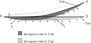
   Figure 4. 2-dimensional picture of intersections of convexhulls of circles $\mu$ and $\omega$, which is represented in the figure by points $\{x,y\}$ and $\{x,z\}$, respecively. The line between x and y represents the convex hull of $\mu$, $C(\mu)$ and the line between x and z represents the convex hull of $\omega$, $C(\omega)$.

   Now WLOG assume $\mu$ lies on the downside of $\omega$. Consider the sequences of least area disks converging to the transverse intersection, $P_{i}\rightarrow L$, and $S_{j}\rightarrow K$ as in the proof of Claim 1. Then again we can fix one disc, $S_{j_{0}}$ in one of the sequences and take another disc, $P_{i}$ intersecting the first one,very close to $L$ and the boundary of $P_{i}$ is very far from the $S_{j_{0}}$’s boundary. Remember by choice of the lamination, $\partial(S_{j})\subset\partial^{-}(N_{c}(C(\mu)$ and $\partial(P_{i})\subset\partial^{-}(N_{c}(C(\omega)$. By Lemma 5.2. $P_{i}\cap T\subset N_{c}(\partial P_{i})$. Then if we choose i sufficiently large $P_{i}$ cannot intersect $\partial S_{j_{0}}\subset T$. But this is a contradiction because if $P_{i}$ intersect $S_{j_{0}}$ transversely, $P_{i}$ must intersect $\partial S_{j_{0}}$      

   

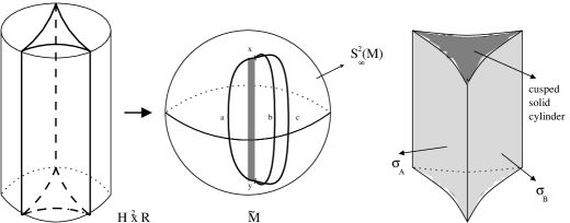
   Figure 5. $A,B,C\in\lambda^{\pm}$ 3 lines and they induce 3 circles in $S^{2}_{\infty}(\tilde{M})$, say $C_{A},C_{B},C_{C}$ where represent the circles through points [x,a,y,b,x],[x,b,y,c,x],[x,c,y,a,x] respectively. When you span these circles at infinity with laminations $\sigma_{A},\sigma_{B},\sigma_{C}$ then there will be an infinite cusped solid cylinder, which is lift of cusped solid torus, between $\sigma_{A},\sigma_{B},\sigma_{C}$.

3. The lamination $\hat{\sigma}^{+}$ is $\pi_{1}$-invariant. i.e. for any $\alpha\in G_{M}$, $\alpha(\hat{\sigma}^{+}_{\omega})=\hat{\sigma}^{+}_{\alpha(\omega)}$.
   

   Proof:  Let $\omega\in\{C^{+}_{x}\}$. Then by definition, $\hat{\sigma}^{+}_{\omega}=\lim\beta_{n}(\hat{\sigma}^{+}_{\tau})$ and $\hat{\sigma}^{+}_{\alpha(\omega)}=\lim\gamma_{n}(\hat{\sigma}^{+}_{\tau})$ where $\lim\beta_{n}(\tau)=\omega$ and $\lim\gamma_{n}(\tau)=\alpha(\omega)$. But, as we showed before, the definitions of $\hat{\sigma}^{+}_{\omega}$ and $\hat{\sigma}^{+}_{\alpha(\omega)}$ are independent of the choice of sequences, and clearly $\lim(\alpha(\beta_{n}))(\tau)=\alpha(\omega)$. This means $\hat{\sigma}^{+}_{\alpha(\omega)}=\lim(\alpha(\beta_{n}))(\hat{\sigma}^{+}_{\tau})$, i.e. $\alpha(\hat{\sigma}^{+}_{\omega})=\hat{\sigma}^{+}_{\alpha(\omega)}$.      

     

So, by the $\pi_{1}$-invariance of the laminations, when we project down the lamination via covering projection, we will get laminations $\Lambda^{\pm}$ in $M$. In other words, if $\pi:\tilde{M}\rightarrow M$ is covering projection, then $\Lambda^{\pm}=\pi(\hat{\sigma}^{\pm})$.

Theorem 5.3.

$\Lambda^{\pm}$ are a pair of transverse genuine laminations.

Proof:  First, we will prove $\Lambda^{+}$ is essential. Each leaf $L_{x}$ of $\Lambda^{+}$ lifts to a surface $\tilde{L}_{x}$ in $\tilde{M}$ which is a least area plane, so $L_{x}$ is incompressible. An end compression of $L_{x}$ would imply the existence of a monogon in $\tilde{M}$ connecting two very close together subdisks of $\tilde{L}_{x}$ of very much larger area, contradicting the fact that $\tilde{L}_{x}$ is least area as in Figure [3]. So, $\Lambda^{+}$ is essential.

Now, if we show that $\Lambda^{+}$ has gut regions, then we are done. If we look at the lift of the lamination $\Lambda^{+}$, which is ${\hat{\sigma}}^{+}$, the lift of the complementary regions, are the complementary regions of ${\hat{\sigma}}^{+}$. Consider that the family of circles $\{C^{+}_{x}\}$ are canonically coming from the lamination $\{\lambda^{+}_{x}\}$ in ${\mathbf{H}}^{2}$. By [Ca], there are some complementary regions which are ideal polygons in ${\mathbf{H}}^{2}$. The image of the leaves in the boundary of this polygonal regions are going to be union of circles such that one of them lies inside the other ones and each circle has at least 2 other circles with nontrivial intersection.see figure [5].

Then the region between these circles will be asymptotic boundary of a complementary region. Clearly, such a region cannot induce a interstitial bundle, so it must be gut region. So, $\Lambda^{+}$ is a genuine lamination.      

Remark 5.1.

This additional hypothesis of transverse orientability is really necessary to work out this proof. It is because when you have 2 circles at infinity which intersects in an interval and their downsides and upsides don’t match up (i.e. the upside of one of them is the downside of the other one.), then the converging disks always intersects nontrivially no matter what happens, when there are least area planes in the laminations spanning these 2 circles. So we cannot get a contradiction as above. See Figure[6].

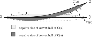
Figure 6. 2-dimensional picture of convex hulls of intersecting 2 circles at infinity whose negative sides don’t match.

6. Topological Pseudo-Anosov Flows

In this section we will show that by using the laminations defined in previous section we could get a Topological pseudo-Anosov flow (TPAF)in the sense of Mosher.

In [Mo], Mosher defined TPAF and he proved that if there is dynamic branced surface pairs in 3-manifold M , then we can induce a TPAF. We will show the branched surfaces carrying the laminations defined in previous section are actually a dynamic pair,and by [Mo] we can induce a TPAF. The following definitions are from [Mo].

Definition 6.1.

$\Phi$ is a TPAF if $\Phi$ has weak stable and unstable foliations, singular along a collection of pseudohyperbolic orbits, and $\Phi$ has a Markov partition which is expansive in a certain sense (the latter condition is just relaxation of the expansive and contracting nature of smooth pseudo-Anosov flows.).

This definition has two main purposes: First, it reflects many of the essential dynamic features of a smooth pseudo-Anosov flow and and so many topological results about smooth pseudo-Anosov flows still hold. Second, it is much easier to verify in specific cases, like ours.

Definition 6.2.

A Dynamic Pair of Branched Surfaces on a compact, closed 3-manifold M, is a pair of branched surfaces $B^{s},B^{u}\subset M$ in general position, disjoint from $\partial M$, together with a $C^{0}$ vector field V on M, so that the following conditions are satisfied.

1. $(B^{s},V)$ and $(B^{u},V)$ are stable and unstable dynamic branched surfaces. (i.e. V is tangent to $B^{s}$ and $B^{u}$ and along branch locus of $B^{u}$, $\Upsilon B^{u}$, points forward (from 2-sheeted side to 1-sheeted side and at crossing point 3-sheeted quadrant to 1-sheeted quadrant) and along branch locus of $B^{s}$, $\Upsilon B^{s}$, points backward (from 1-sheeted side to 2-sheeted side and at crossing point 1-sheeted quadrant to 3-sheeted quadrant))

2. V is smooth on M, except along $\Upsilon B^{s}$ where backward trajectories locally unique, and along $\Upsilon B^{u}$ where forward trajectories locally unique.

3. Each component of $M-(B^{s}\cup B^{u})$ is either a pinched tetrahedron or a solid torus. In solid torus piece, V is circular. See Fig[??]

4. Each component of $B^{u}-B^{s}$ and $B^{s}-B^{u}$ is an annulus with cusped tongues, see figure[??]. On components of $B^{u}-B^{s}$,the annulus is a sink for V (all forward trajectories of V after a time is in the annulus.), and similarly on components of $B^{s}-B^{u}$,the annulus is a source for V (all backward trajectories of V after a time is in the annulus.).

5. No two solid torus components of $M-(B^{s}\cup B^{u})$ are glued to each other, i.e. the closures of solid torus components are disjoint.

Now, let $\Lambda^{\pm}$ be the genuine laminations defined in previous section. Let $B^{\pm}$ be the branched surfaces carrying $\Lambda^{\pm}$. We want to show that $B^{\pm}$ are dynamic pair. Here, $B^{+}$ and $B^{-}$ correspond to $B^{s}$ and $B^{u}$, respectively.

Lemma 6.1.

$\Lambda^{\pm}$ are very full laminations in M, i.e. gut regions are solid tori.

Proof:  This is true as the gut regions are coming from the ideal polygons of the lamination $\lambda^{\pm}\subset S^{1}_{i}nfty({\mathbf{H}}^{2}$. These ideal polygons induces circles at infinity as in the Figure[5]. So the gut regions are the region between the lamination spanning this circles. On the other hand for each ideal polygon we have an element $\alpha$ in $\pi_{1}(M)$ fixes this ideal polygon (the topological pseudo-Anosov elements in [Ca]). Then $\alpha$ fixes the two common points of all the circles coming from the each side of ideal polygon. So, the gut region must be a solid tori whose core is homotopic to the element $\alpha$. So, the gut regions are solid tori.      

Now, recall that the lamination $\Lambda^{\pm}$ is coming from universal cover and the lifting laminations $\tilde{\Lambda^{\pm}}$ are laminations by least area planes. Let P be a least area plane in the lamination and let $\partial_{\infty}(P)=\tau\in\{C^{+}_{x}\}$. Then we have special point $a\in\tau\subset S^{2}_{\infty}(\tilde{M})$. By Lemma 2.4, $\tau=q\circ p(\partial_{\infty}(l^{+}_{x}\times I)))$ and by proof we know that $q\circ p(\partial(l^{+}_{x})\times I\cup l^{+}_{x}\times\{\infty\})$is a point and we define this point as special point in $\tau$.

Let $B^{\pm}$ branched surfaces carrying the genuine laminations $\Lambda^{\pm}$ such that branch locus of $B^{\pm}$ is transverse to the $B^{+}\cap B^{-}$.

Theorem 6.2.

If $B^{\pm}$ branched surfaces carrying the genuine laminations $\Lambda^{\pm}$ then $B^{\pm}$ are a dynamic pair of branched surfaces. So, there is a topological pseudo-Anosov flow on M by [Mo].

Proof:  There are 5 steps.

1. (Structure of $B^{\pm}$ and M)
   $M-B^{+}$ is union of cusped tori, $Q^{+}_{i}$. Similarly, $M-B^{-}$ is also union of cusped tori, $Q^{-}_{i}$. Moreover $Q^{+}_{i}\cap Q^{-}_{i}=T_{i}$ where $T_{i}$ represents solid torus gut region for $\Lambda^{\pm}$. $M-(B^{+}\cup B^{-})$ consists of solid tori ( not cusped) and pinched tetrahedron Figure[7].On the other hand, components of $B^{+}-B^{-}$ and $B^{-}-B^{+}$ are annuli with ”cusped” tongues as in the figure [6].
   

   

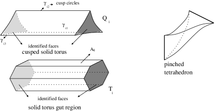
   Figure 7. Shapes of cusped solid torus and pinched tetrahedron pieces in $M-(B^{+}\cup B^{-})$. Solid torus gut region is intersection of 2 transverse cusped solid torus pieces.

   Since $\Lambda^{\pm}$ are very full laminations, then $M-B^{+}=\bigcup_{i=1}^{n}Q_{i}^{+}$ where $Q_{i}^{+}$ represents cusped solid torus piece, see Figure [7]. similarly $M-B^{-}=\bigcup_{i=1}^{n}Q_{i}^{-}$. Moreover for any i, $Q_{i}^{+}\cap Q_{i}^{-}=T_{i}$ where $T_{i}$ is the (noncusped) solid torus gut piece of the lamination. As we have seen above, these gut regions, $T_{i}$, comes from $r_{i}$ sided ideal polygons in $\lambda^{\pm}$, as we call them $r_{i}-prong$. Then these cusped torus pieces, $Q_{i}^{\pm}$ have $r_{i}$ cusp circles, say $\gamma^{\pm}_{ij}$ $1\leq j\leq r_{i}$. In the boundary of corresponding gut region $T_{i}$, there are $2r_{i}$ parallel circles, coming from the intersection $Q_{i}^{+}\cap Q_{i}^{-}=T_{i}$. These $2r_{i}$ circles in the boundary of solid tori $T_{i}$, bounds $2r_{i}$ annuli in $\partial(T_{i})$ and these annuli alternatingly in $B^{+}$ and $B^{-}$. if it is in $B^{+}$, we will call them $+annulus$ and if it is in $B^{-}$ then we will call them $-annulus$.

   

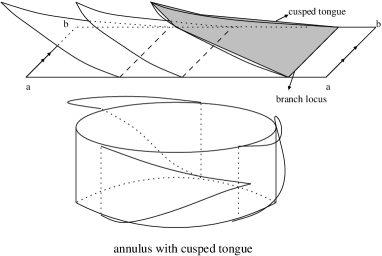
   Figure 8. Shape of annulus with 3 cusped tongues.

   Take a $+annulus$ in $\partial(T_{i})$. This annulus comes from the intersection of a cusp in $Q^{-}_{i}$ and $B^{+}$. So we can index these annuli, by just considering the indexing of cusps coming from $\gamma^{\pm}_{ij}$. So for each $+annulus$ there is a $\gamma^{-}_{ij}$ and for each $-annulus$, there is a $\gamma^{+}_{ij}$. Then call the $+annuli$ corresponding to $\gamma^{-}_{ij}$ as $A^{+}_{ij}$ and similarly define $A^{-}_{ij}$. Now, we have $\partial(T_{i})=\cup_{j=1}^{r_{i}}A^{+}_{ij}\bigcup\cup_{j=1}^{r_{i}}A^{-}_{ij}$.

   Each cusp circle $\gamma^{-}_{ij}$ and $A^{+}_{ij}$ defines a cusp, say $C^{-}_{ij}$, in $Q^{-}_{ij}$ and similarly $C^{+}_{ij}$, in $Q^{+}_{ij}$. Then the cusped solid torus $Q^{-}_{i}=T_{i}\bigcup\cup_{j=1}^{r_{i}}C^{-}_{ij}$ and similarly $Q^{+}_{i}=T_{i}\bigcup\cup_{j=1}^{r_{i}}C^{+}_{ij}$ See Figure[9].

   

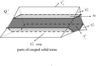
   Figure 9. $Q_{i}^{+}=T_{i}\cup(\bigcup_{j=1}^{3}C_{ij}^{+})$

   Now, let’s describe the pieces of $B^{+}-B^{-}$. we claim that these pieces are annuli with ”cusped” tongues as in the figure [8]. Consider $M-B^{+}=\bigcup_{i=1}^{n}Q_{i}^{+}$. then $\bigcup_{i=1}^{n}\partial(Q_{i}^{+})\supseteq B^{+}$. So if we understand, how +cusped tori and -cusped tori intersect, then we can easily decribe the components of $B^{+}-B^{-}$. But as we mentioned above, these intersections produce solid tori gut regions and cusps. This means that components of $B^{+}-B^{-}$ will have one of annulus $A^{+}_{ij}$ and the remaining part of the component will be in the cusp $C^{+}_{ij}$. It is easy to see that these parts in the cusp will be the cusped tongues coming from the other sections of the branched surface $B^{+}$ as in the Figure [8] (section of a branched surface is the components of branched surface - branch loci, $B^{+}-\Upsilon B^{+}$).

   The other claim is that the components of $M-(B^{+}\cup B^{-})$ are solid tori and pinched tetrahedra. Consider the following trivial set theoretic equivalences. $M-(B^{+}\cup B^{-})=(M-B^{+})\bigcap(M-B^{-})=(\bigcup_{i=1}^{n}Q_{i}^{+})\bigcap(\bigcup_{i=1}^{n}Q_{i}^{-})=(\bigcup_{i=1}^{n}(Q_{i}^{+}\cap Q_{i}^{-}))\bigcup(\bigcup_{i\neq k}(Q_{i}^{+}\cap Q_{k}^{-}))=(\bigcup_{i=1}^{n}T_{i})\bigcup(\bigcup_{i\neq k}(Q_{i}^{+}-T_{i})\cap(Q_{k}^{-}-T_{k}))=(\bigcup_{i=1}^{n}T_{i})\bigcup(\bigcup_{ij\neq kl}C_{ij}^{+}\cap C_{kl}^{-})$

   Now, the first part of the union comes from the equality $Q_{i}^{+}\cap Q_{i}^{-}=T_{i}$, intersection of cusped solid tori with same indices is the corresponding solid torus gut region. In the latter part of the union we just used the definitions in the first paragraph: $Q_{i}^{+}-T_{i}=\bigcup_{j=1}^{r_{i}}C_{ij}^{+}$, the cusped solid tori are the union of solid tori gut regions and the cusps.

   So, if we can understand $C_{ij}^{+}\cap C_{kl}^{-}$ for i and k different, then we will finish this step. we claim that this intersections give us the pinched tetrahedra components. Consider the Figure [10]. As it can be seen there the intersection of the cusps of different cusped solid tori is in general position (by assumption, $\tau=B^{+}\cap B^{-}$ is transverse to the branch loci of the branched surfaces, $\Upsilon B^{\pm}$.). Fix a cusp $C_{ij}^{+}$ in $Q_{i}^{+}$. Now, consider the intersection of $C_{ij}^{+}$ with the other regions. Obviously, since this region lives already in the complement of $B^{+}$, $\bigcup_{i=1}^{n}Q_{i}^{+}$ , no region in the complement of $B^{+}$ intersect $C_{ij}^{+}$. Now, consider the intersection with $\bigcup_{i=1}^{n}Q_{i}^{-}$. Since solid tori gut regions are disjoint from cusps then only cusps of the negative cusped solid tori will intersect our region $C_{ij}^{+}$.

   

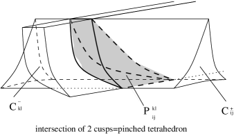
   Figure 10. Intersection of 2 cusps, $C_{ij}^{+}\cap C_{kl}^{-}$, is a pinched tetrahedron, $P_{ij}^{kl}$.

   Recall that the cusps are topologically just a cusped (in one vertex) triangle $\times S^{1}$. the cusp vertex $\times S^{1}$ corresponds cusp circle which is in branch locus of $B^{+}$, $\Upsilon B^{+}$, and the opposite side of triangle $\times S^{1}$ corresponds the annulus in $B^{-}$. Now the negative cusps intersect our cusp circle in intervals and the annulus have some interval parts of branch locus of $B^{-}$. These intervals will constitute the cusped sides of a tetrahedra intersections, and the intersections of positive and negative cusps will be pinched tetrahedra. So, the components of $M-(B^{+}\cup B^{-})$ are solid tori and pinched tetrahedra as claimed.
   

2. We can define vector field X on M which is tangent to $\tau=B^{+}\cap B^{-}$ and $B^{+}$ and $B^{-}$.
   

   First, we will define the vector field on train track $\tau=B^{+}\cap B^{-}$ and then we will extend first to $B^{+}-B^{-}$ and $B^{-}-B^{+}$ naturally.
   

   • X on $\tau$:
     

     It is not obvious that we can define a vector field on a train track, see Figure[11].

     

     Figure 11. we cannot define a vector field on this train track.

     This is indeed same thing with orienting each segment in train track consistently. First we will show that we can define canonically a vector field on $\tau$ by using the circles at infinity in universal cover. If we consider the lift of branched surfaces in universal cover $\tilde{B^{\pm}}$, we can see the the intersection train track lifts to infinite lines asymptotic to the end of lifts of solid tori, which are the special points (defined above) of corresponding circles at infinity, i.e. each infinite line limits to one positive special point (special point in a positive circle $C^{+}_{x}$ at infinity) and to one negative special point ( to see intuitively consider the quasi-isometric picture of $\tilde{M}$ as $\mathbf{H}^{2}\times\mathbf{R}$, and the infinite lines starts from bottom disk and ends in top disk) So clearly we can orient each infinite line from a negative special point to positive special point. Now, we will induce consistent orientation of each segment of $\tau$ using these orientation of lines in $\tilde{\tau}$. Take a line segment $I\subset\tau$ and consider a lift of this line segment $\tilde{I}\subset\tilde{\tau}$ in universal cover. Clearly, we can orient the circles in $\tau$ which are in boundary of solid torus gut regions (for each $T_{i}$, there are $2r_{i}$ circles in $\partial(T_{i})$ which are also in $\tau$) parallel to the core of the gut region.

     Now the only remaining part of $\tau$ to orient is the line segments connecting these circles. Consider the the quasi-isometric picture of $\tilde{M}$ as $\mathbf{H}^{2}\times\mathbf{R}$. In this picture as we have seen in Section 2, the family of circles at infinity $\{C^{\pm}\}$, comes from $\partial_{\infty}(\lambda^{\pm}\times\mathbf{R})$ by collapsing $\lambda^{+}$ in $\mathbf{H}^{2}\times\{+\infty\}$ and by collapsing $\lambda^{-}$ in $\mathbf{H}^{2}\times\{-\infty\}$.Since $B^{\pm}$ carries the laminations $\Lambda^{\pm}$ (i.e. $\Lambda^{\pm}\subset N_{\epsilon}(B^{\pm})$),$\partial_{\infty}(\Lambda^{\pm})=\partial_{\infty}(B^{\pm}))$. So, if you take two ”close” leaves of lifts of $\tilde{B}^{+}$ they will intersect in an interval not containing their special point of both circles and they will start to differ from their special point (Recall that every circle at infinity, $\{C^{\pm}\}$, has a special point which is the image of the endpoint of corresponding leave of $\lambda^{\pm}$) See Figure[12]. This is true for $\tilde{B}^{-}$ as well. So, for the circles corresponding to the sides of ideal polygons in $\lambda^{\pm}$ and corresponding circle at infinity of the leaves in $\tilde{B}^{\pm}$ containing boundaries of solid tori gut regions, they have both negative and positive special points, and as in previous paragraph we oriented the core of solid torus as from negative special point to positive special point. See Figure[13]

     

     Figure 12. Induced circles from 3 generic leaves, $l_{x},l_{y},l_{z}\in\lambda^{+}$ (not a boundary of ideal polygon in the complement of $\lambda^{+}$) in $S^{2}_{\infty}(\tilde{M})$

     

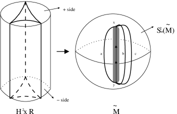
     Figure 13. Induced circles from 3 nongeneric leaves, $l_{a},l_{b},l_{c}\in\lambda^{+}$ (sides of ideal polygon in the complement of $\lambda^{+}$) in $S^{2}_{\infty}(\tilde{M})$

     Now, observe that in $\mathbf{H}^{2}\times\mathbf{R}$ picture, the lift of branch locus, $\tilde{\Upsilon}^{+}$ (which are lines as loops in branch locus are essential), in $\tilde{B}^{+}$ branches towards positive side of $\mathbf{H}^{2}\times\mathbf{R}$, and similarly, $\tilde{\Upsilon}^{-}$ in $\tilde{B}^{-}$ branches towards negative side of $\mathbf{H}^{2}\times\mathbf{R}$, see figure [14]. This is very easy to see if the laminations are geodesic planes in $\mathbf{H}^{2}\times\mathbf{R}$, because of the tightness. But in our situtation the tightness comes from being least area planes, which works in our situation as well. In other words, we know that the close circles at infinity, say $C^{+}_{1},C^{+}_{2}$ starts to diverge from each other from their special points and this will cause inside $\tilde{M}$ the leaves $L_{1},L_{2}$ of lamination $\Lambda^{+}$ will be close to each other for some time but they will start to diverge from each other after a lift of intersititial annulus. See figure [15]. On the other hand this intersititial annulus corresponds in branched surface literature a branch locus. Now, we want to say that this branchings towards upside for $B^{+}$ and towards downside for for $B^{-}$. This is true as at infinity diverging starts at positive side and inside we have tightness coming from the lamination being by least area planes.

     Now, let’s come back to $\tau$. For a line segment in $\tau$ starts from $\Upsilon B^{+}$ and ends in $\Upsilon B^{-}$ will be as in Figure[16] . So we will orient this line segment from $\Upsilon B^{+}$ to $\Upsilon B^{-}$. Then our quasi-isometric picture of $\tilde{M}$ as $\mathbf{H}^{2}\times\mathbf{R}$ shows that the orientation on each line of $\tilde{\tau}$ is coherent, and when we project it to the original manifold, we can easily get a vector field on our train track $\tau$.
     

     

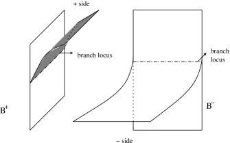
     Figure 14. Shape of neighborhood of $\tilde{\Upsilon B^{\pm}}$ in $\tilde{B^{\pm}}$ in $\mathbf{H}^{2}\times\mathbf{R}$ picture of $\tilde{M}$.

     

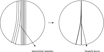
     Figure 15. 2 dimensional picture of laminations and branched surfaces carrying them. Intersititial annulus becomes branch locus.

   • Extending X to the components of $B^{+}-B^{-}$ and $B^{-}-B^{+}$:
     

     By the first step we know that the components are annuli with cusped tongues. Now fix a component. Then its boundary will be in $\tau$, and we already defined X on $\tau$. Now, as we pointed before, since we induced X on $\tau$ from universal cover’s boundary at infinity, there is no consistency problem. i.e. since X is well-defined on $\tau$, on the boundary of annulus of component, they must be parallel, and on boundary of cusped tongues they are consistent. So we can easily extend first on annulus such that each integral integral curve of X on annulus is closed as in boundary (as X is parallel on two circles of the boundary), and then on cusped tongues. If we have a +annulus with cusped tongue then X on $\tau$ points away from the ideal vertex towards the annulus, and we can extend X to the cusped tongue with integral curves starting at ideal vertex, tangent to the sides contatining ideal vertex, and ending in the opposite side of ideal vertex, which is a segment of $\Upsilon B^{-}$. Similarly, we can extend X to -annulus with cusped tongue.
     

   • Extending X to whole manifold by defining on the solid torus and pinched tetrahedron pieces.
     

     We have defined X on whole $B^{\pm}$. As we proved before components of $M-(B^{+}\cup B^{-})$ are solid tori and pinched tetrahedra. First, let’s extend X to pinched tetrahedron pieces. Fix a pinched tetrahedron P. $\partial P$ consists of 4 cusped tongues, one couple comes from a positive annulus with cusped tongues (the component is in $B^{+}-B^{-}$) and the other couple comes from negative annulus with cusped tongues(the component is in $B^{-}-B^{+}$). Now, there are 2 cusped segments in P, one is an interval $I^{+}$ in $\Upsilon B^{+}$, and the other is an interval $I^{-}$ in $\Upsilon B^{-}$. Now, by our definition of X on $\tau$, and it’s canonical extension to the components of $B^{+}-B^{-}$ and $B^{-}-B^{+}$, X points inside to P on $I^{+}$ and points outside from P on $I^{-}$. Then, it is clear that we can extend X to whole P such that, X will be tangent to $\partial P$ and any integral curve of X in P starts from $I^{+}$ and ends in $I^{-}$.

     

     Figure 16. Orienting the train track $\tilde{\tau}$

     Now, fix a solid torus $T_{i}$ in $M-(B^{+}\cup B^{-})$. As above, $\partial T_{i}$ consists of $2r_{i}$ annuli from $B^{\pm}$. Boundaries of these annuli are $2r_{i}$ closed curves in $\tau$, and the definition of X on these annuli canonically comes from the definition of X on these circles. But, we defined X on $\tau$ by using the lift of $T_{i}$ to universal cover, and on each of these closed curves on $\partial T_{i}$ X is parallel to the orientation of the core curve of $T_{i}$. So on each annuli the integral curves of X are closed and have same orientation with the core curve of $T_{i}$. It is obvious that we can simply extend X to $T_{i}$ such that each integral curve is closed and oriented parallel to core curve (i.e. the integral curves on solid torus $T_{i}$ will be the trivial one dimensional foliation.).

     Now, we have to check that X is continuous on M, i.e. there is no consistency problem with the definition of X on different components. Since there cannot be any problem inside the pinched tetrahedron and solid torus pieces, we should check only the boundaries of these pieces which are $B^{+}\cup B^{-}$. But already we have induced X from the boundaries of the pieces, X is also continuous on the boundaries, i.e. $B^{+}\cup B^{-}$. So, X is a $C^{0}$ vector field on M and it is tangent to $B^{+}\cup B^{-}$, such that X points inside to $B^{-}$ on $\Upsilon B^{-}$ and points outside from $B^{+}$ on $\Upsilon B^{+}$.
     

3. There is no face gluings between solid torus gut regions, $T_{i}$, i.e. torus pieces of $M-(B^{+}\cup B^{-})$ are separated.
   

   Assume there is a face gluing between two solid torus components, say $T_{i},T_{j}$. This means there is a common annulus piece in $\partial(T_{i})\cap\partial(T_{j})$. When we look at the lifts of $T_{i}$ and $T_{j}$ to the universal cover, we see that there is only one plane component of the lift of $B^{+}$ or $B^{-}$ separating these two lifts $\tilde{T_{i}}$ and $\tilde{T_{j}}$. On the other hand, that means the boundary at infinity of this plane is isolated in both sides. This is not hard see, as these solid tori components comes from ideal polygons in the lamination of circle $\lambda^{\pm}$. See figure[17].

   

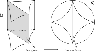
   Figure 17. Face gluings implies isolated leaves. Left ideal triangle of $\lambda^{+}\subset S^{1}_{\infty}$ induce one cusped solid torus, and right ideal triangle induce the other cusped solid torus.

   But this is contradiction since isolated circle at the boundary at infinity means isolated leaf of the lamination $\lambda^{\pm}$ and we already know by [Ca] that $\lambda^{\pm}$ has no isolated leaves.
   

4. $B^{\pm}$ are dynamic pair of branched surfaces.
   

   The steps 1, 2, 3 proves the first 5 conditions of dynamic pair of branched surfaces and the step 4 shows the last condition of dynamic pair of branched surfaces. So, $B^{\pm}$ are dynamic pair of branched surfaces.

     

This means if M is an atoroidal 3-manifold admitting uniform 1-cochain, then there is a TPAF on M induced by the uniform 1-cochain. If we consider uniform 1-cochains as generalization of sliterings this is a generalization of a theorem of Thurston [Th]: if an atoroidal 3-manifold M slithers around circle then there is a pseudo-Anosov flow on M, transverse to the uniform foliationinduced by slithering. In our setup, the uniform foliation corresponds the coarse foliation of $\tilde{M}$ induced by uniform 1-cochain.

7. Concluding Remarks

The transverse orientability condition on uniform 1-cochain is a little bit strong and disturbing. To get rid of this hypothesis, one can try different approaches. One of them could be the below conjecture.

Conjecture: Let M be Gromov hyperbolic 3-manifold, and $\alpha$ and $\beta$ are two simple closed curves in $S^{2}_{\infty}(\tilde{M})$. If the least area planes K, and L spanning $\alpha$ and $\beta$, respectively, intersect transversely in a line l which limits $\{x,y\}\subset S^{2}_{\infty}(\tilde{M})$, then the circles $\alpha$ and $\beta$ intersect transversely at $\{x,y\}$.

This might seem a very optimistic conjecture because in one less dimension this is not true, as geodesics may intersect and stay in bounded Hausdorff distance in Gromov hyperbolic manifolds. But, 2-dimensionality of the objects might be very crucial and essential here. If this conjecture was true, the above theorem would follow easily as the planes in laminations would automatically be pairwise disjoint. Moreover, this conjecture would make this technique so powerful that to get an essential lamination in Gromov hyperbolic manifolds would be equivalent to get a $\pi_{1}(M)$ invariant family of circles at infinity.

On the other hand, the minimal surface techniques and results in this paper are indeed original in the sense that it starts with an algebraic condition on fundamental group $\pi_{1}(M)$, like admitting a function to $\mathbf{R}$, uniform 1-cochain, and ends up with two real topological object in the manifold M, like genuine laminations and topological pseudo-Anosov flow. Of course, most of the work has been done by Calegari in his beautiful paper [Ca].

In last five years, we have seen three breakthrough results of nonexistence of some promising structures in 3-manifolds. Roberts, Shareshian, and Stein proved that there are hyperbolic manifolds without taut foliations, [RSS]. By that time, it was believed that taut foliations are very abundant in 3-manifolds, it might even be enough for weak hyperbolization. By [RSS], we saw that this is not true. The next promising structure for weak hyperbolization was essential laminations. Calegari and Dunfield showed that tight essential laminations in atororidal manifolds induce circle action of the fundamental group and the fundamental group of the Weeks manifold does not act on circle. So this is the first example of hyperbolic manifolds without tight essential laminations. Finally, Fenley showed that there are hyperbolic manifolds without any essential laminations, [Fe]. Taut foliations and essential laminations were expected to provide a positive answer for weak hyperbolization before these results.

Similarly, after Thurston’s paper on slitherings, [Th], then their generalization as uniform 1-cochains by Calegari, and abundance of bounded 1-cochains by geometric group theory, uniform 1-cochains might also be considered as a promising tool for weak hyperbolization. The above paper of Calegari and Dunfield also show that there are hyperbolic manifolds without uniform 1-cochains. Since uniform 1-cochains on atoroidal manifolds induce faithful circle action of fundamental group by [Ca], they showed that the fundamental group of the Weeks manifold does not act on circle, so Weeks manifold cannot admit uniform 1-cochain.

When we started this problem, [CD] and [Fe] were not published yet, and we believed that by proving these results, we can contribute to Thurston’s and Calegari’s promising program for weak hyperbolization. After [CD] and [Fe], one can look at our results as another way of proving nonexistence of uniform 1-cochains in some hyperbolic manifolds, up to transverse orientability condition. This is because by our work transversely orientable uniform 1-cochains induce genuine laminations and by [Fe], there are hyperbolic manifolds without genuine laminations.

References

- [Ca] D. Calegari, Bounded cochains on 3-manifolds, eprint; math.GT/0111270
- [Ca2] D. Calegari, The geometry of -covered foliations, Geom. Top. 4 (2000), 457-515, math.GT/9903173
- [CD] D. Calegari and N. Dunfield, Laminations and groups of homeomorphisms of the circle , eprint; math.GT/0203192
- [CM] T. Colding and W.P. Minicozzi, Minimal surfaces, Courant Lecture Notes in Mathematics, 4, 1999.
- [CT] J. Cannon and W. Thurston, Group Invariant Peano Curves, preprint.
- [Fe] S. Fenley, Laminar free hyperbolic 3-manifolds, eprint; math.GT/0210482.
- [Ga] D. Gabai, On the geometric and topological rigidity of hyperbolic -manifolds, J. Amer. Math. Soc. 10 (1997), no. 1, 37–74.
-
[Ge]
S. Gersten A cohomological characterization of hyperbolic groups,
http://www.math.utah.edu/ gersten/Papers/ch.pdf, preprint. - [GO] D. Gabai and U. Oertel, Essential Laminations in 3-manifolds, Ann. of Math. (2) 130 (1989), 41–73.
- [HS] J. Hass and P. Scott, The Existence of Least Area Surfaces in 3-manifolds, Trans. AMS 310 (1988), 87–114.
- [Ma] J. Manning, Geometry of Pseudocharacters, eprint; math.GR/0303380
- [Mo] L. Mosher, Laminations and flows transverse to finite depth foliations, Part I: Branched surfaces and dynamics., http://newark.rutgers.edu/ mosher/, preprint.
- [RSS] R. Roberts, J Shareshian, and M. Stein, Infinitely many hyperbolic 3-manifolds which contain no Reebless foliation to appear in J. Amer. Math. Soc., http://www.math.wustl.edu/ roberts/research.html, preprint.
- [S] R. Schoen, Estimates for Stable Minimal Surfaces in Three Dimensional Manifolds, Ann. of Math. Stud. 103 (1983), 111–126.
- [Th] W. Thurston, Three-manifolds, Foliations and Circles, I, eprint; math.GT/9712268
- [Th2] W. Thurston, Hyperbolic structures in 3-manifolds II, eprint; math.GT/9801045