Vanishing and non-vanishing criteria in Schubert calculus

Abstract

For any complex reductive connected Lie group $G$, many of the structure constants of the ordinary cohomology ring $H^{*}(G/B;\mathbb{Z})$ vanish in the Schubert basis, and the rest are strictly positive. We present a combinatorial game, the “root game”, which provides some criteria for determining which of the Schubert intersection numbers vanish. The definition of the root game is manifestly invariant under automorphisms of $G$, and under permutations of the classes intersected. Although these criteria are not proven to cover all cases, in practice they work very well, giving a complete answer to the question for $G=SL(7,\mathbb{C})$. In a separate paper we show that one of these criteria is in fact necessary and sufficient when the classes are pulled back from a Grassmannian.

More generally If $G^{\prime}\hookrightarrow G$ is an inclusion of complex reductive connected Lie groups, there is an induced map $H^{*}(G/B)\to H^{*}(G^{\prime}/B^{\prime})$ on the cohomology of the homogeneous spaces. The image of a Schubert class under this map is a positive sum of Schubert classes on $G^{\prime}/B^{\prime}$. We investigate the problem of determining which Schubert classes appear with non-zero coefficient. This is the vanishing problem for branching Schubert calculus, which plays an important role in representation theory and symplectic geometry, as shown in [Berenstein-Sjamaar 2000]. The root game generalises to give a vanishing criterion and a non-vanishing criterion for this problem.

1 Introduction

In this paper we introduce some techniques for studying vanishing problems in Schubert calculus. The most basic and famous such problem concerns the cohomology ring of a generalised flag manifold $G/B$: we would like to determine combinatorially which of the structure constants for $H^{*}(G/B)$ are non-zero. We refer to this as the vanishing problem for multiplication in Schubert calculus. However, the techniques we introduce here apply in a more general context, namely to the vanishing problem for branching Schubert calculus—discussed below—of which the multiplication problem is a special case. Although it is possible to calculate any structure constants for these problems explicitly (e.g. using Schubert polynomials [BH]), the known methods involve alternating sums, and thus provide little insight into the question of which terms vanish. A complete combinatorial solution to either of these problems is still not known.

Our first objective is to provide some vanishing and non-vanishing criteria for intersection numbers of Schubert varieties on $G/B$. Geometrically, the problem is this: given $s\geq 3$ Schubert varieties in general position, determine whether or not their intersection is empty. If we know the Schubert intersection numbers we also implicitly have the Schubert structure constants for $H^{*}(G/B)$ (from the Poincaré pairing), thus this also addresses the vanishing problem for multiplication.

In Section 3, we introduce the root game which can often give information about a Schubert intersection number. In some circumstances the root game will tell us that the intersection number is $0$ (Theorem 1); in other circumstances, the game will tell us that the intersection number is at least $1$ (Theorem 2). Unfortunately, in a few cases, the root game gives no information; remarkably though, for $G=SL(n)$, $n\leq 7$ we have confirmed by computer that all of these remaining cases have intersection number $0$.

The rules of the root game are manifestly symmetric under permutations of the classes intersected, as well as under automorphisms of $G$. Furthermore, once the game has been fully internalized, it is highly amenable to computations by hand.

Our second objective is to show that the main results hold in an even more general setting, which we call branching Schubert calculus. Let $i:G^{\prime}\hookrightarrow G$ be an inclusion of complex reductive connected Lie groups. Choose Borel subgroups $B^{\prime}\subset G$ and $B\subset G$ such that $i(B^{\prime})\subset B$. Then we obtain an inclusion $i:G^{\prime}/B^{\prime}\hookrightarrow G/B$ (which we also denote by $i$, in a mild abuse of notation). Hence there is a map on cohomology $i^{*}:H^{*}(G/B)\to H^{*}(G^{\prime}/B^{\prime})$. The problem of branching Schubert calculus is to determine the map $i^{*}$ in the Schubert basis, i.e. given a Schubert class $\omega\in H^{*}(G/B)$ we would like to express $i^{*}(\omega)\in H^{*}(G^{\prime}/B^{\prime})$ in the Schubert basis of the latter.

The coefficients which appear in such an expression are always non-negative integers. Although there are formulae for these integers, it is not known how to determine them combinatorially, or even how to determine which terms appear. In Section 4, we investigate the latter problem, and obtain some widely applicable criteria for determining which terms appear.

The vanishing problem for branching Schubert calculus generalises the vanishing problem for multiplication in Schubert calculus: if $i:G^{\prime}\hookrightarrow G=G^{\prime}\times G^{\prime}$ is the diagonal inclusion, then the map $i^{*}$ is just the cup product in cohomology. Similarly, multiplication of more than two terms comes from considering the diagonal inclusion $G^{\prime}\hookrightarrow G^{\prime}\times\cdots\times G^{\prime}$.

Our motivation for this work comes from [BS], in which Berenstein and Sjamaar use the vanishing problem for branching Schubert calculus to answer questions in symplectic geometry and representation theory. Let $K^{\prime}$ and $K$ be the maximal compact subgroups of $G^{\prime}$ and $G$ respectively. Berenstein and Sjamaar use the vanishing problem for branching Schubert calculus to calculate the $K^{\prime}$ moment polytope of a $K$-coadjoint orbit. They show that each non-vanishing branching coefficient gives rise to an inequality satisfied by the moment polytope. Moreover, all together, the complete list of non-vanishing branching coefficients gives a sufficient set of inequalities for this polytope.

This symplectic problem is to be equivalent to an asymptotic version of a fundamental representation theory question, as shown in [H, GS] (for more of this picture see also [GLS]). Let $\lambda$ and $\mu$ be dominant weights for $G$ and $G^{\prime}$ respectively. Let $V_{\lambda}$ denote the irreducible $G$-representation with highest weight $\lambda$; similarly let $V^{\prime}_{\mu}$ denote the irreducible $G^{\prime}$-representation with highest weight $\mu$. When $V_{\lambda}$ is decomposed as a $G^{\prime}$-module, it is a basic question whether a component of type $V^{\prime}_{\mu}$ appears. The asymptotic version of this problem is the following: does there exists a positive integer $N$, such that the $G$-module $V_{N\lambda}$ has a component of type $V^{\prime}_{N\mu}$, when decomposed as a $G^{\prime}$-module? The answer is yes if and only if the point $\mu$ lies in the $K^{\prime}$-moment polytope for the $K$-coadjoint orbit through $\lambda$. Thus the non-vanishing branching coefficients give an answer to this asymptotic representation theory question as well.

In studying the vanishing problem for branching Schubert calculus, we will actually be considering the following apparently simpler problem: determine which Schubert classes are in the kernel of $i^{*}$. While this may at first seem to be a vast simplification, it is in fact equivalent to the original problem, as shown by Proposition 2.2. In the case of vanishing for multiplication of Schubert classes, this is a familiar fact: we can determine which structure constants of the cohomology ring are zero, based on the which triple products vanish.

The paper begins with a discussion of the geometry underlying the root games (section 2). The basic idea is to use Kleiman’s Bertini theorem [Kl] to reduce the vanishing problem to a transversality problem in the tangent space to a point in $G/B$. Given an intersection in the tangent space, we attempt to show it is transverse by degenerating it to a position where transversality is easily verifiable. If this is possible, we can conclude that that a corresponding Schubert class is not in the kernel of $i^{*}$.

The degenerations in question can be encoded combinatorially; doing so gives the root game. In Section 3, we introduce the root game for Schubert intersection numbers. Section 4 contains the more general root game for branching Schubert calculus, and proofs of the main theorems. Ultimately it is the proof of Theorems 4 and 5, which tie the combinatorics into the geometry.

We refer the reader to [F] for a general reference on type $A$ Schubert calculus, and to [BH] for the other classical Lie groups.

The author is deeply grateful to Allen Knutson, for providing a lot of helpful feedback on this paper.

2 Geometry of vanishing problem for branching Schubert calculus

2.1 Conventions

Given $i:G^{\prime}\hookrightarrow G$, an inclusion of complex reductive connected Lie groups, we wish to study the map $i^{*}:H^{*}(G/B)\to H^{*}(G^{\prime}/B^{\prime})$. First, we need to demonstrate that the derived map $i:G^{\prime}/B^{\prime}\hookrightarrow G/B$ always exists.

Proposition 2.1.

Given $i:G^{\prime}\hookrightarrow G$ there exist Borel subgroups $B^{\prime}\subset G^{\prime}$ and $B\subset G$ such that $i(B^{\prime})\subset B$.

Proof.

Choose a Borel subgroup $B_{0}\subset G$, and consider the $G^{\prime}$-orbits on $G/B_{0}$ of minimal dimension. Each such orbit is closed, therefore, compact, and so is $G^{\prime}/P$ for some parabolic subgroup $P\subset G^{\prime}$. Choose a point ${x_{0}}$ on such an orbit. The stabiliser of ${x_{0}}$ inside $G^{\prime}$, $G^{\prime}_{x_{0}}$, is conjugate to $P$, whereas the stabiliser of ${x_{0}}$ inside $G$, $G_{x_{0}}$, is conjugate to $B_{0}$. Thus $G^{\prime}_{x_{0}}\subset G_{x_{0}}$ is solvable, but $G^{\prime}/G^{\prime}_{x_{0}}$ is compact, hence $G^{\prime}_{x_{0}}$ is a Borel subgroup of $G^{\prime}$. We take $B=G_{x_{0}}$ and $B^{\prime}=G^{\prime}_{x_{0}}$. ∎

Let $T^{\prime}\subset B^{\prime}$ be a maximal torus of $G^{\prime}$. Extend its image $i(T^{\prime})$ to a maximal torus $T\subset B$ of $G$. Let $N^{\prime}$ and $N$ denote the corresponding unipotent subgroups of $B^{\prime}$ and $B$. Of course, $i(N^{\prime})\subset N$. Henceforth we will simply view $T^{\prime}$, $N^{\prime}$, $B^{\prime}$ as subgroups of $T$, $N$, $B$ respectively.

Let $\Delta$ denote the root system of $G$, and $\Delta^{\prime}$ the root system of $G^{\prime}$. The positive and negative roots of $\Delta$ (with respect to the choice of $B$) are denoted $\Delta_{+}$ and $\Delta_{-}$ respectively. For each root $\alpha\in\Delta$, we fix a basis vector $e_{\alpha}$ for the corresponding root space in $\mathfrak{g}$. Likewise, for each root $\beta\in\Delta^{\prime}$, we fix a basis vector $e^{\prime}_{\beta}$ for the corresponding root space in $\mathfrak{g}^{\prime}$.

The tangent spaces to ${x_{0}}$ in $G/B$ and $G^{\prime}/B^{\prime}$ are naturally are $\mathfrak{g}/\mathfrak{b}$ and $\mathfrak{g}^{\prime}/\mathfrak{b}^{\prime}$ respectively. Thus linearising $i$ gives a a natural inclusion of tangent spaces $\mathfrak{g}^{\prime}/\mathfrak{b}^{\prime}\hookrightarrow\mathfrak{g}/\mathfrak{b}$. We use the Killing form to identify $\mathfrak{n}$ with $(\mathfrak{g}/\mathfrak{b})^{*}$. Similarly, we identify the dual of $\mathfrak{g}^{\prime}/\mathfrak{b}^{\prime}$ with $\mathfrak{n}^{\prime}$. Thus we obtain a linear map

$$\phi:\mathfrak{n}\to\mathfrak{n}^{\prime}$$

which is adjoint to the inclusion of tangent spaces $\mathfrak{g}^{\prime}/\mathfrak{b}^{\prime}\hookrightarrow\mathfrak{g}/\mathfrak{b}$. Essentially $\phi$ encodes all the information about the inclusion $G^{\prime}\hookrightarrow G$.

Note that since ${x_{0}}$ is a $T^{\prime}$-fixed point, the map $\phi$ is $T^{\prime}$-equivariant. Thus, it takes the $T$-weight spaces to $T^{\prime}$-weight spaces, and induces a map

$$\hat{\phi}:\Delta_{+}\to\Delta^{\prime}_{+}\cup\{0\}$$

defined by the rule

$$\hat{\phi}(\alpha)=\begin{cases}0,&\text{if $\phi(e_{\alpha})=0$}\\ \beta,&\text{where $0\neq\phi(e_{\alpha})$ is in the $\beta$-weight space.}\end{cases}$$

In Section 4 we will need to consider subsets $\mathcal{T}\subset\Delta_{+}$ with the following properties.

Definition 2.1.

Suppose $\mathcal{T}\subset\Delta_{+}$ satisfies

1. $0\notin\phi(\mathcal{T})$, and
2. $\hat{\phi}|_{\mathcal{T}}$ is injective.

We call such a subset $\mathcal{T}$ injective. Equivalently $\mathcal{T}\subset\Delta_{+}$ is injective if $\phi|_{\langle e_{\alpha}\,|\,\alpha\in\mathcal{T}\rangle}$ is an injective linear map.

2.2 Schubert varieties

Let $W=N(T)/T$ be the Weyl group of $G$. For $\pi\in W$, let $[\pi]$ denote the corresponding $T$-fixed point on $G/B$, and let $\tilde{\pi}$ denote some lifting of $\pi\in W$ to an element of $N(T)\subset G$.

Let $w_{0}$ denote the long element in $W$. For $\pi\in W$, let $\pi^{\prime}=w_{0}\pi$. To each $\pi\in W$ we associate the Schubert cell $X^{\circ}_{\pi}=B\cdot[\pi^{\prime}]$, the $B$-orbit through $[\pi]$ in $G/B$. Its closure $X_{\pi}=\overline{B\cdot[\pi^{\prime}]}$, is the Schubert variety. (This definition is slightly non-standard: it is more common to define $X_{\pi}=\overline{B_{-}\cdot[\pi]}$, where $B_{-}$ is an opposite Borel. Our $X_{\pi}$ is a translation of the more standard one by $\tilde{w}_{0}$.) According to these conventions $X_{1}=G/B$ (where $1\in W$ represents the identity element) and $X_{w_{0}}=\{x_{0}\}$. In general $X_{\pi}$ is a complex subvariety of $G/B$ whose codimension is length of $\pi\in W$ (denoted $\ell(\pi)$).

Let $\omega_{\pi}$ denote the cohomology class Poincaré dual to the homology class of the Schubert variety $X_{\pi}$, that is the class such that

$$\int_{X_{\pi}}\sigma=\int_{G/B}\omega_{\pi}\cdot\sigma$$

for all $\sigma\in H^{*}(G/B)$. Since the the codimension of $X_{\pi}$ is $\ell(\pi)$, $\omega_{\pi}$ is a cohomology class of degree $2\ell(\pi)$. The class $\omega_{1}\in H^{*}(G/B)$ is the (multiplicative) identity element.

The following proposition shows that the vanishing problem for branching Schubert calculus is equivalent to the problem of determining whether $\omega_{\pi}\in\ker i^{*}$.

Proposition 2.2.

Given $j:G^{\prime}\hookrightarrow G^{\prime\prime}$ an inclusion of complex reductive connected groups, let $G=G^{\prime}\times G^{\prime\prime}$ and $i=(id\times j)\circ\delta:G^{\prime}\hookrightarrow G$, where $\delta:G^{\prime}\to G^{\prime}\times G^{\prime}$ is the diagonal map. Let $i^{*}:H^{*}(G/B)\cong H^{*}(G^{\prime}/B^{\prime})\times H^{*}(G^{\prime\prime}/B^{\prime\prime})\to H^{*}(G^{\prime}/B^{\prime})$ be the induced map on cohomology. A Schubert class $\sigma\in H^{*}(G^{\prime}/B^{\prime})$ appears in the expansion of $j^{*}(\omega)$ if and only if $(\sigma^{\vee},\omega)\notin\ker i^{*}$, and $\deg\sigma^{\vee}+\deg\omega=\dim_{\mathbb{R}}G^{\prime}/B^{\prime}$. Here $\sigma^{\vee}$ is the Schubert class dual to $\sigma$ under the Poincaré pairing .

Proof.

Consider the integral

$$\int_{G^{\prime}/B^{\prime}}\sigma^{\vee}\cdot j^{*}(\omega).$$

If this integral is non-zero, then $\sigma$ appears in the expansion of $j^{*}(\omega)$ (with coefficient equal to $\int_{G^{\prime}/B^{\prime}}\sigma^{\vee}\cdot j^{*}(\omega)$); otherwise it does not.

Since $i=(id\times j)\circ\delta$, we have $i^{*}(\sigma^{\vee},\omega)=\delta^{*}(\sigma^{\vee},j^{*}(\omega))=\sigma^{\vee}\cdot j^{*}(\omega)$, thus

$$\int_{G^{\prime}/B^{\prime}}\sigma^{\vee}\cdot j^{*}(\omega)=\int_{G^{\prime}/B^{\prime}}i^{*}(\sigma^{\vee},\omega).$$

The second integral is clearly non-zero if and only if $(\sigma^{\vee},\omega)\notin\ker i^{*}$ and $\deg\sigma^{\vee}+\deg\omega=\dim_{\mathbb{R}}G^{\prime}/B^{\prime}$. ∎

Thus, to solve the vanishing problem for branching Schubert calculus for $j:G^{\prime}\hookrightarrow G^{\prime\prime}$, it is sufficient to know whether $i^{*}(\sigma^{\vee},\omega)=0$, for any given $(\sigma^{\vee},\omega)\in H^{*}(G/B)$.

Henceforth we shall be investigating the question of whether $i^{*}(\omega_{\pi})=0$, for $\pi\in W$. We will assume that $\pi\in W$ is an element whose length $\ell(\pi)\leq\dim G^{\prime}/B^{\prime}$: if $\ell(\pi)>\dim G^{\prime}/B^{\prime}$ then $i^{*}(\omega_{\pi})=0$ for dimensional reasons. We are primarily interested in the case where $\ell(\pi)=\dim G^{\prime}/B^{\prime}$, however except where specified otherwise, everything in this paper holds for all $\pi\in W$.

2.3 The multiplication problem

A special and particularly important case is the vanishing problem for multiplication of Schubert calculus. As mentioned, in the introduction, this corresponds to the diagonal inclusion $G^{\prime}\hookrightarrow G=G^{\prime}\times\cdots\times G^{\prime}$ ($s$-factors).

In this case, a Schubert class $\omega_{\pi}\in H^{*}(G/B)$ can be regarded as an $s$-tuple of Schubert classes $(\omega_{\pi_{1}},\ldots,\omega_{\pi_{s}})\in(H^{*}(G^{\prime}/B^{\prime}))^{s}$. The map $i^{*}:H^{*}(G/B)\to H^{*}(G^{\prime}/B^{\prime})$ gives the product of these Schubert classes in $H^{*}(G^{\prime}/B^{\prime})$:

$$i^{*}(\omega_{\pi})=i^{*}(\omega_{\pi_{1}},\ldots,\omega_{\pi_{s}})=\omega_{\pi_{1}}\cdots\omega_{\pi_{s}}.$$

Thus the problem of determining when $i^{*}(\omega_{\pi})\neq 0$ becomes the question of which collections of Schubert classes on $G^{\prime}/B^{\prime}$ have non-vanishing product.

We are most interested in the case where $\ell(\pi)=\sum\ell(\pi_{i})=\dim(G^{\prime}/B^{\prime})$. In this case we are investigating the Schubert intersection numbers $c_{\pi_{1}\ldots\pi_{s}}$ defined by

$$c_{\pi_{1}\ldots\pi_{s}}=\int_{G^{\prime}/B^{\prime}}\omega_{\pi_{1}}\cdots\omega_{\pi_{s}}.$$

The triple Schubert intersection numbers $c_{\pi_{1}\pi_{2}\pi_{3}}$ are particularly important, as they are the Schubert structure constants of the cohomology ring $H^{*}(G/B)$. Indeed, if we write

$$\omega_{\pi_{1}}\cdot\omega_{\pi_{2}}=\sum_{\rho\in W}c_{\pi_{1}\pi_{2}}^{\rho}\omega_{\rho}$$

then

$$c_{\pi_{1}\pi_{2}\pi_{3}} =\int_{G/B}\omega_{\pi_{1}}\cdot\omega_{\pi_{2}}\cdot\omega_{\pi_{3}}$$

$$=\int_{G/B}\sum_{\rho\in W}c_{\pi_{1}\pi_{2}}^{\rho}\omega_{\rho}\cdot\omega_{\pi_{3}}$$

$$=c_{\pi_{1}\pi_{2}}^{w_{0}\pi_{3}}.$$

2.4 Tangent space methods

The main idea behind the results in this paper is to use Kleiman’s theorem [Kl] to translated problems of intersection theory on $G/B$ into transversality questions on the tangent space to $G/B$. Tangent space methods have been used elsewhere in the literature, perhaps most notably in Belkale’s geometric proof of the Horn conjecture [B]. Our main lemma (Lemma 2.4) generalises some of these ideas.

Lemma 2.3.

Let $x\in G/B$. The following conditions are equivalent:

1. $i^{*}(\omega_{\pi})\neq 0$,

2. There exist $g_{1},g_{2}\in G$ such that $x\in g_{1}X^{\circ}_{\pi}\cap g_{2}G^{\prime}/B^{\prime}$, and the tangent spaces $T_{x}g_{1}X_{\pi}$ and $T_{x}g_{2}G^{\prime}/B^{\prime}$ are transverse linear subspaces of $T_{x}G/B$.

Proof.

We apply Kleiman’s Theorem to the $G$-homogeneous space $G/B$ and its subvarieties $X_{\pi}$ and $G^{\prime}/B^{\prime}$. Consider the intersections

$$I_{g_{1},g_{2}}=g_{1}X_{\pi}\cap g_{2}G^{\prime}/B^{\prime}$$

and

$$I^{\circ}_{g_{1},g_{2}}=g_{1}X^{\circ}_{\pi}\cap g_{2}G^{\prime}/B^{\prime}\,.$$

If $g_{1},g_{2}$ are generic elements of $G$, Kleiman’s theorem tells us that a generic point $\tilde{x}$ of $I_{g_{1},g_{2}}$ is a smooth point of $g_{1}X_{\pi}$ which can be assumed to lie in $g_{1}X^{\circ}_{\pi}$; moreover the varieties $g_{1}X^{\circ}_{\pi}$ and $g_{2}G^{\prime}/B^{\prime}$ are transverse at $\tilde{x}$. In particular $I_{g_{1},g_{2}}$ is generically reduced and equidimensional. If $I_{g_{1},g_{2}}$ is zero-dimensional then $I_{g_{1},g_{2}}$ is finite, with cardinality $\#(I_{g_{1},g_{2}})=\int_{G^{\prime}/B^{\prime}}i^{*}(\omega_{\pi})$. More generally $I_{g_{1},g_{2}}$ defines a homology class in $G^{\prime}/B^{\prime}$ which is Poincaré dual to to the cohomology class $i^{*}(\omega_{\pi})$. In particular, we have that $i^{*}(\omega_{\pi})\neq 0$ if and only if $I_{g_{1},g_{2}}$ (or equivalently $I^{\circ}_{g_{1},g_{2}}$) is nonempty for generic $(g_{1},g_{2})\in G\times G$.

Let $A=\{(g_{1},g_{2})\ |\ I^{\circ}_{g_{1},g_{2}}\neq\emptyset\}$. (Note $G^{\prime}\times G^{\prime}\subset A$ so $A$ is always non-empty.) We have just shown $\bar{A}=G\times G$ if and only if $i^{*}(\omega_{\pi})\neq 0$. Let $(g_{1},g_{2})$ be a generic point of $A$ (If $A$, is reducible choose any component), and $\tilde{x}\in I_{g_{1},g_{2}}$ be a generic point of $I_{g_{1},g_{2}}$. If $i^{*}(\omega_{\pi})\neq 0$ then $(g_{1},g_{2})$ is in fact a generic point of $G\times G$ and so the varieties $g_{1}X_{\pi}$ and $g_{2}G^{\prime}/B^{\prime}$ are transverse at $\tilde{x}$. However, note that the set

$$\{(g_{1},g_{2})\ |\ \text{$g_{1}X^{\circ}_{\pi}$ and $g_{2}G^{\prime}/B^{\prime}$ have a transverse point of intersection}\}$$

is necessarily open (intuitively this is because a transverse intersection remains transverse under perturbation). Thus, conversely, if $g_{1}X_{\pi}$ and $g_{2}G^{\prime}/B^{\prime}$ are transverse at $\tilde{x}$, then $\bar{A}=G\times G$ and hence $i^{*}(\omega_{\pi})\neq 0$.

Finally, since $G$ acts transitively on $G/B$, we can find $g\in G$ such that $g\tilde{x}=x$. Then $g_{1}X_{\pi}$ and $g_{2}G^{\prime}/B^{\prime}$ are transverse at $\tilde{x}$ iff $gg_{1}X_{\pi}$ and $gg_{2}G^{\prime}/B^{\prime}$ are transverse at $x$. This completes the proof. ∎

Lemma 2.3 is still not concrete enough for our purposes. We reformulate it as follows.

For $a\in N$, let $a\cdot\ :\mathfrak{n}\to\mathfrak{n}$ denote the adjoint action of $N$ on its Lie algebra. Let $Q\subset\mathfrak{n}$ be the subspace generated by the $e_{\alpha}$ such that $\alpha\in\Delta_{+}$ and $\pi^{-1}\cdot\alpha\in\Delta_{-}$. Equivalently,

$$Q=\mathfrak{n}\cap(\pi\cdot\mathfrak{b}_{-}).$$

Lemma 2.4.

The following are equivalent:

1. $i^{*}(\omega_{\pi})\neq 0$.

2. $\phi|_{a\cdot Q}$ is injective for some $a\in N$.

3. $\phi|_{a\cdot Q}$ is injective for generic $a\in N$.

The tangent space to $G/B$ at $x_{0}$ is naturally $\mathfrak{g}/\mathfrak{b}$. We identify the cotangent space $(\mathfrak{g}/\mathfrak{b})^{*}$ with $\mathfrak{n}$ using the Killing form. Under these identifications, $Q^{\perp}\simeq((\pi^{\prime}\cdot\mathfrak{b})+\mathfrak{b})/\mathfrak{b}$. The subspace $a\cdot Q\subset\mathfrak{n}$ is identified with the conormal space at the point $x_{0}$ to a translated Schubert variety $g\cdot X_{\pi}\ni x_{0}$. Thus Lemma 2.4 is essentially a dual statement to Lemma 2.3.

Proof.

The equivalence of conditions 2 and 3 is clear, as the maps $\phi|_{A}$ are injective for a Zariski open set of subspaces $A$.

To show the equivalence of 1 and 3, we use Lemma 2.3 with the point $x=x_{0}$.

We have $x_{0}\in g\cdot X^{\circ}_{\pi}$ if and only if $g=b_{1}(\tilde{\pi}^{\prime})^{-1}$ for some $b_{1}\in B$, and $x_{0}\in g^{\prime}G^{\prime}/B^{\prime}$ if and only if $g^{\prime}=b_{2}h$, for $b_{2}\in B$, $h\in G^{\prime}$. Put $b=b_{2}^{-1}b_{1}$, and write $b=at$, with $a\in N$, and $t\in T$.

Then,

$$T_{x_{0}}gX_{\pi}\cap T_{x_{0}}g^{\prime}G^{\prime}/B^{\prime} =b_{2}\cdot\big{(}b\cdot T_{x_{0}}(\tilde{\pi}^{\prime})^{-1}X_{\pi}\cap T_{x_{0}}G^{\prime}/B^{\prime}\big{)}$$

$$=b_{2}\cdot\big{(}(b\cdot(\pi^{\prime}\cdot\mathfrak{b})+\mathfrak{b})/\mathfrak{b}\cap\mathfrak{g}^{\prime}/\mathfrak{b}^{\prime}\big{)}$$

$$=b_{2}\cdot\big{(}(b\cdot Q)^{\perp}\cap\mathfrak{g}^{\prime}/\mathfrak{b}\big{)}$$

$$=b_{2}\cdot\big{(}(a\cdot Q)^{\perp}\cap\mathfrak{g}^{\prime}/\mathfrak{b}\big{)}$$

The transversality of the intersection $(a\cdot Q)^{\perp}\cap\mathfrak{g}^{\prime}/\mathfrak{b}$ is precisely the dual statement to condition (2). ∎

Applied to the multiplication problem, Lemma 2.4 reduces to the following.

Corollary 2.5.

Let $Q_{i}=\mathfrak{n}^{\prime}\cap(\pi_{i}\cdot\mathfrak{b}^{\prime}_{-})$ be the subspace of $\mathfrak{n}^{\prime}$ whose weights are the inversion set of $\pi_{i}$. Then the following are equivalent:

1. $c_{\pi_{1}\ldots\pi_{s}}\neq 0$,

2. The sum of subspaces $a_{1}\cdot Q_{1}+\cdots+a_{s}\cdot Q_{s}$ is a direct sum, for generic choices of $a_{i}\in N$.

2.5 Necessary conditions for vanishing

Our first consequence of Lemma 2.4 is the vanishing criterion.

Lemma 2.6.

Let $S\subset\mathfrak{n}$ be an $N$-submodule of $\mathfrak{n}$. If $\dim\phi(S)<\dim(Q\cap S)$, then $i^{*}(\omega_{\pi})=0$.

Proof.

As $S$ is $N$-invariant, we have that

$$\dim((a\cdot Q)\cap S)=\dim(Q\cap S)>\dim\phi(S)$$

for all $a\in N$. It follows that $\phi|_{((a\cdot Q)\cap S)}$ is not injective, and thus $\phi|_{a\cdot Q}$ is not injective. Therefore, by Lemma 2.4, $i^{*}(\omega_{\pi})=0$. ∎

Moreover, if we take $S$ to be a $B$-submodule of $\mathfrak{n}$ then there are only finitely many possibilities, and we can readily calculate the dimensions of $\phi(S)$ and $Q\cap S$ combinatorially. This is essentially the content of Theorem 4.

Remark 2.2.

From Lemma 2.6, it is possible to rederive the necessary Horn inequalities for non-vanishing of Schubert calculus on Grassmannians. For more on this picture, see [P3].

2.6 Degenerating $Q$

To show $i^{*}(\omega_{\pi})\neq 0$, by Lemma 2.4, it is enough to exhibit a subspace $U=a\cdot Q$ in the $N$-orbit through the subspace $Q$ such that $\phi|_{U}$ is injective. Actually, because the set

$$\{U\in Gr(\dim G^{\prime}/B^{\prime},\mathfrak{n})\ |\ \phi|_{U}\text{is injective}\}$$

is open, we can take $U$ to be in the closure of the $N$-orbit through $Q$. Note that since $Q$ is a $T$-fixed subspace of $\mathfrak{n}$, the $B$-orbit through $Q$ coincides with the $N$-orbit through $Q$.

The idea behind obtaining sufficient conditions is to look for a $T$-fixed subspace of $\mathfrak{n}$, $U\in\overline{B\cdot Q}$, such that $\phi|_{U}$ is injective. We can think of the search for a suitable $U$ as a process. Beginning with the $T$-fixed subspace $Q\subset V$ we degenerate to another $T$-fixed subspace $U\in\overline{B\cdot Q}$. If $\phi|_{U}$ is not injective, we can degenerate further inside $\overline{B\cdot U}$, until a suitable subspace is found.

Let $V=\mathfrak{n}$ or any $B$-module subquotient of $\mathfrak{n}$. Let $V^{\prime}=\mathfrak{n}$ or any $B^{\prime}$-module subquotient of $\mathfrak{n}^{\prime}$. Suppose we have a $B^{\prime}$-equivariant map $\psi:V\to V^{\prime}$

Let $Gr(V)$ denote the disjoint union of all Grassmannians

$$Gr(V)=\coprod_{l=0}^{\dim V}Gr_{l}(V).$$

Since $V$ has a $B$-action, so does $Gr(V)$.

Let $U\in Gr(V)$ be a subspace of $V$. We call the quadruple $(U,V,V^{\prime},\psi)$ good if there is a point $\tilde{U}\in\overline{B\cdot U}$ such that $\psi|_{\tilde{U}}:\tilde{U}\to V^{\prime}$ is an injective linear map. Note that the set of ${\tilde{U}}\in Gr(V)$ with $\phi|_{\tilde{U}}$ injective is Zariski open in $Gr(V)$. Thus, equivalently, $(U,V,V^{\prime},\psi)$ is good if there exists $\tilde{U}\in B\cdot U$ such that $\psi|_{\tilde{U}}:{\tilde{U}}\to V^{\prime}$ is an injective linear map.

In the language of good quadruples, Lemma 2.4 states that $i^{*}(\omega_{\pi})=0$ if and only if the quadruple $(Q,\mathfrak{n},\mathfrak{n}^{\prime},\phi)$ is good.

2.6.1 Moving between fixed points

For any $T$-representation $U$ with distinct weights, let $\Gamma(U)$ denote the set of weights of $U$.

To every $\beta\in\Delta_{+}$, we can associate a one dimensional unipotent subalgebra $N_{\beta}\subset N$, whose Lie algebra $\mathfrak{n}_{\beta}$ is $T$-invariant with weight $\beta$. $N_{\beta}$ is isomorphic to the additive Lie group $\mathbb{C}$. Let $\theta_{\beta}:\mathbb{C}=N_{\beta}\hookrightarrow N$ denote the inclusion of groups, $\theta_{\beta}(t)=\exp te_{\beta}$.

The following proposition is a triviality, yet it is at the very heart of the root game.

Proposition 2.7.

Let $U\in Gr(V)$, and let $U^{1}=\lim_{t\to\infty}\theta_{\beta}(t)\cdot U$. If $(U^{1},V,V^{\prime},\psi)$ is good, then $(U,V,V^{\prime},\psi)$ is good.

Proof.

The point $(U^{1},V,V^{\prime},\psi)$ lies in the closure of $\overline{B\cdot U}$. Thus if there exists $\tilde{U}\in\overline{B\cdot U^{1}}$ such that $\psi|_{\tilde{U}}$ is injective, then $\tilde{U}$ also lies in $\overline{B\cdot U}$. ∎

Remark 2.3.

In particular if $\psi|_{U^{1}}$ happens to be injective then $(U,V,V^{\prime},\psi)$ is good. Otherwise we can attempt to apply Proposition 2.7 recursively to $(U^{1},V,V^{\prime},\psi)$, to show that $(U^{1},V,V^{\prime},\psi)$ is good and hence that $(U,V,V^{\prime},\psi)$ is good.

Suppose now that $U$ is a $T$-fixed point of $Gr(V)$. We show that $U^{1}$ is a $T$-fixed point of $Gr(V)$ and calculate the weights $\Gamma(U^{1})$ in terms of $\Gamma(U)$.

Definition 2.4.

Call an element $\alpha\subset\Gamma(U)$ $\beta$-shiftable, if there is a positive integer $k$ such that $\alpha+k\beta\in\Gamma(V)\setminus\Gamma(U)$. Let $\Gamma(U)\boxplus_{\Gamma(V)}\beta$ denote the set

$$\{\alpha+\beta\ |\ \text{$\alpha$ is $\beta$-shiftable}\}\ \cup\ \{\alpha\ |\ \text{$\alpha$ is not $\beta$-shiftable}\}$$

Lemma 2.8.

Let $U^{1}=\lim_{t\to\infty}\theta_{\beta}(t)\cdot U$. Then $U^{1}$ is a $T$-fixed point of $Gr(V)$ and $\Gamma(U^{1})=\Gamma(U)\boxplus_{\Gamma(V)}\beta$.

Proof.

Let $\bar{e}_{\alpha}\in V$ be a vector with weight $\alpha$. Since the weights of $V$ are distinct, we can represent $U$ as $[\bar{e}_{\alpha_{1}}\wedge\ldots\wedge\bar{e}_{\alpha_{l}}]$, and $U^{1}$ as $[\bar{e}_{\alpha^{\prime}_{1}}\wedge\ldots\wedge\bar{e}_{\alpha^{\prime}_{l}}]$, via the Plücker embedding $Gr(V)\hookrightarrow P(\bigwedge^{*}V)$. Now

$$\theta_{\beta}(t)\cdot U =\theta_{\beta}(t)\cdot[\bar{e}_{\alpha_{1}}\wedge\ldots\wedge\bar{e}_{\alpha_{l}}],$$

$$=\big{[}(\bar{e}_{\alpha_{1}}+t(e_{\beta}\cdot\bar{e}_{\alpha_{1}}))\wedge\ldots\wedge(\bar{e}_{\alpha_{l}}+t(e_{\beta}\cdot\bar{e}_{\alpha_{l}}))\big{]}$$

$$=\sum_{C\subset\{1,\ldots,l\}}t^{|C|}\pm\bigwedge_{i\in C}e_{\beta}\cdot\bar{e}_{\alpha_{i}}\wedge\bigwedge_{i\in C^{c}}\bar{e}_{\alpha_{i}}$$

(here $e_{\beta}\cdot$ is the action of $\mathfrak{n}_{\beta}$ on $V$ induced from the adjoint action). Now up to a non-zero constant multiple,

$$e_{\beta}\cdot\bar{e}_{\alpha_{i}}=\begin{cases}\bar{e}_{\alpha_{i}+\beta},&\text{if $\alpha_{i}+\beta\in\Gamma(V)$}\\ $0$,&\text{otherwise.}\end{cases}$$

This is a property of the adjoint representation which $V$, as subquotient of the adjoint representation, inherits.

We see that a summand is non-zero only if $\{\alpha_{i}\ |\ i\in C\}$ is a subset of the set of $\beta$-shiftable weights of $\Gamma(U)$. In the limit as $t\to\infty$, the only term which survives is the one with the highest power of $t$, which is precisely

$$[\pm t^{\text{\#$\beta$-shiftable weights}}\bar{e}_{\alpha^{\prime}_{1}}\wedge\ldots\wedge\bar{e}_{\alpha^{\prime}_{l}}].$$

∎

2.6.2 Splitting into two smaller problems

Let $S\subset V$ be an $B$-submodule, and $S^{\prime}\subset V$ an $B^{\prime}$-submodule. Suppose that $\psi(S)\subset S^{\prime}$. Let $q:V\to V/S$ and $q^{\prime}:V^{\prime}\to V^{\prime}/S^{\prime}$ denote the quotient maps.

From the quadruple $(U,V,V^{\prime},\psi)$ and the submodules $S,S^{\prime}$, we obtain two induced quadruples: they are $(U\cap S,S,S^{\prime},\psi|_{S})$, and $(q(U),V/S,V^{\prime}/S^{\prime},\psi_{q})$, where $\psi_{q}:=q^{\prime}\circ\psi\circ q^{-1}$. (Note that $\psi_{q}:V/S\to V^{\prime}/S^{\prime}$ is well defined.)

Proposition 2.9.

If $(U\cap S,S,S^{\prime},\psi|_{S})$, and $(q(U),V/S,V^{\prime}/S^{\prime},\psi_{q})$ are both good, then $(U,V,V^{\prime},\phi)$ is good.

Proof.

Let $p:Gr(V)\to Gr(S)$ be the map $p(U)=U\cap S$, and note that $q$ also defines a similar map $q:Gr(V)\to Gr(V/S)$. Note that $p$ and $q$ are not continuous everywhere, but since $S$ is a $B$-submodule, they are $B$-equivariant and continuous on $B$-orbits.

Define

$$g(U,V,V^{\prime},\psi):=\{\tilde{U}\in B\cdot U\subset Gr(V)\ |\ \text{$\psi|_{\tilde{U}}$ is injective}\}.$$

Let $g_{p}=g(U\cap S,S,S^{\prime},\psi|_{S})$ and $g_{q}=g(q(U),V/S,V^{\prime}/S^{\prime},\psi_{q})$. If $(U\cap S,S,S^{\prime},\psi|_{S})$, and $(q(U),V/S,V^{\prime}/S^{\prime},q^{\prime}\circ\psi\circ q^{-1})$ are good, then $g_{p}$ and $g_{q}$ are respectively dense subsets of the $B$-orbits $B\cdot p(U)\subset Gr(S)$ and $B\cdot q(U)\subset Gr(V/S)$. By $B$-equivariance of $p$ and $q$, $p^{-1}(g_{p})\cap B\cdot U$ and $q^{-1}(g_{q})\cap B\cdot U$ are both dense subsets of $B\cdot U\subset Gr(V)$.

Take $\tilde{U}\in p^{-1}(g_{p})\cap q^{-1}(g_{q})$. Then $\psi|_{p(\tilde{U})}:\tilde{U}\cap S\to S^{\prime}$ and $\psi_{q}|_{q(\tilde{U})}:q(\tilde{U})\to V^{\prime}/S^{\prime}$ are both injective. By elementary linear algebra, $\psi|_{\tilde{U}}:{\tilde{U}}\to V^{\prime}$ is therefore also injective, as required. ∎

2.6.3 Factoring through an intermediate module

In Sections 3 and 4, the geometric ideas in Propositions 2.7 and 2.9 will translate into the combinatorics of the root game. Our next proposition is not used, because it is not so easy to make combinatorial in its full generality. However, a special case of this can be nicely incorporated into the root game for Schubert intersection numbers; this appears in Section 3.5.4.

Given a quadruple $(U,V,V^{\prime},\psi)$, let $\tilde{B}$ be a group such that $B^{\prime}\subset\tilde{B}\subset B$, and let $\tilde{V}$ be a $\tilde{B}$ module. Suppose the map $\psi$ factors as $\psi=\psi_{2}\circ\psi_{1}$, where $\psi_{1}:V\to\tilde{V}$ is $\tilde{B}$ equivariant, and $\psi_{2}:\tilde{V}\to V^{\prime}$ is $B^{\prime}$ equivariant.

Proposition 2.10.

If $\psi_{1}|_{U}:U\to\tilde{V}$ is injective and $(\psi_{1}(U),\tilde{V},V^{\prime},\psi_{2})$ is good, then $(U,V,V^{\prime},\psi)$ good.

Proof.

If there exists $a\in\tilde{B}$ such that $\psi_{2}|_{a\cdot\psi_{1}(U)}$ is injective, then $\psi|_{a\cdot U}$ is also injective. ∎

2.7 Questions

The results of this section (Propositions 2.7, 2.9 and 2.10) provide a way of proving that $i^{*}(\omega_{\pi})\neq 0$, by producing a set of varieties ($B$-orbit closures on Grassmannians $Gr(V)$), and $T$-fixed points $U$ on these varieties such that $\psi|_{U}$ is injective. A natural question is whether such a $T$-fixed point always exists if $i^{*}(\omega_{\pi})=0$.

This question as stated is somewhat vague, and can be phrased more precisely in a couple of different ways. The most obvious interpretation is does there exist a suitable $T$-fixed point which can be found using only the results of this section? Less restrictively, one might observe that successive uses of Proposition 2.7 may not find all the $T$-fixed points on a $B$-orbit. If one includes all the $T$-fixed points in the picture, does a suitable $T$-fixed point always exists? If so how does one practically find these other $T$-fixed points?

The first formulation of the question is essentially asking for a converse to Theorems 2 and 5, and unfortunately the answer is in general no (see Section 3.5.4 for further discussion). The second formulation is open and appears to be a difficult problem. In [P2] we show that the answer is yes for the multiplication problem in the special case where the Schubert classes are pulled back from a Grassmannian.

3 Root games for Schubert intersection numbers

3.1 Overview of the root game

The root game combinatorially encodes the geometric notions of Section 2. We discuss two versions of the game. In this section we will handle the special case of the vanishing problem of Schubert intersection numbers on $G^{\prime}/B^{\prime}$. We present the most general version (for the branching problem of a general inclusion $G^{\prime}\hookrightarrow G$) in Section 4.

The former is actually a special case of the latter. We present the two formulations separately, since several of the rules become simplified in the root game for Schubert intersection numbers, and moreover it is convenient to encode the data slightly differently for these two problems.

The basic overview of the game is the same for both problems. The playing field is a set of squares, which correspond to positive roots of $G$ or $G^{\prime}$. Some of the squares contain tokens, which get moved from square to square by the player according to certain rules. The set of all squares is subdivided into regions, which limit the movement of the tokens. The player alternates between subdividing the regions further (splitting), and moving around tokens, in an attempt to reach a winning position.

In Section 3.3, we shall see the connection with the geometry in Section 2.6. In short, the positions of the tokens will represent the $T$-weights of potential degenerations of the subspace $Q\subset\mathfrak{n}$. The position of the tokens before and after a move will be the weights before and after a degeneration of the type in Proposition 2.7, whereas the splitting of regions corresponds to the type of subdivision in Proposition 2.9. Ultimately the purpose of the game is to search for a degeneration of $Q$ which will allow us to easily conclude that $c_{\pi_{1}\ldots\pi_{s}}\neq 0$ from Lemma 2.4; these will be the winning positions.

We advise the reader who wishes to skip directly to the more general branching root game to glance first at examples 3.1 and 3.9, which illustrate how the squares arranged for root systems of types A and B, as this will be essential to understanding subsequent examples.

3.2 Rules of the game

Recall the problem: given $(\pi_{1}\ldots,\pi_{s})$, the vanishing problem is to determine whether $c_{\pi_{1}\ldots\pi_{s}}=\int_{G^{\prime}/B^{\prime}}\omega_{\pi_{1}}\cdots\omega_{\pi_{s}}=0$. We assume that $\sum\ell(\pi_{i})=\dim G^{\prime}/B^{\prime}$, otherwise this integral vanishes for dimensional reasons.

3.2.1 Data of a position

The position in a root game consists of the following data:

• A partition of the set of positive roots of $G^{\prime}$, i.e. $\mathcal{R}=\{R_{1},\ldots,R_{r}\}$, such that $\Delta^{\prime}_{+}=\coprod_{i=1}^{s}R_{i}$. Each $R_{i}$ is called a region.

• A list of subsets $\mathcal{T}_{1},\ldots,\mathcal{T}_{s}$ of the positive roots of $G^{\prime}$, which we call the arrangement of tokens.

We organise these data as follows. We draw a set of squares: the squares correspond to the positive roots of $G^{\prime}$, and are arranged in a sensible way (depending on the type of $G^{\prime}$.) The squares are denoted $S_{\alpha}$, $\alpha\in\Delta^{\prime}_{+}$.

Example 3.1.

Suppose $G^{\prime}=SL(n)$. Let $x_{1},\ldots,x_{n}$ denote an orthonormal basis for $\mathbb{R}^{n}$. The root system $\Delta^{\prime}=A_{n-1}$ is $\{\alpha_{ij}=x_{j}-x_{i}\ |\ i\neq j\}$. The positive roots are those for which $i<j$. We can view our squares corresponding to the positive roots as being arranged inside an $n\times n$ array of squares. Let $AS_{ij}$ denote the square in position $(i,j)$. The relevant squares are squares $AS_{ij}$ (the square in position $(i,j)$), where $1\leq i<j\leq n$. Thus the positive root $\alpha_{ij}$, with $i<j$ is assigned to the square $AS_{ij}$.

$$\Delta(SL(6))_{+}=(A_{5})_{+}=\text{ \begin{tabular}[]{ccccc}\hline\cr\vrule\lx@intercol\hfil\rule[-8.0pt]{0.0pt}{24.0pt}$\alpha_{12}$\hfil\lx@intercol &\vrule\lx@intercol\hfil\rule[-8.0pt]{0.0pt}{24.0pt}$\alpha_{13}$\hfil\lx@intercol &\vrule\lx@intercol\hfil\rule[-8.0pt]{0.0pt}{24.0pt}$\alpha_{14}$\hfil\lx@intercol &\vrule\lx@intercol\hfil\rule[-8.0pt]{0.0pt}{24.0pt}$\alpha_{15}$\hfil\lx@intercol &\vrule\lx@intercol\hfil\rule[-8.0pt]{0.0pt}{24.0pt}$\alpha_{16}$\hfil\lx@intercol\vrule\lx@intercol \\ \hline\cr&\vrule\lx@intercol\hfil\rule[-8.0pt]{0.0pt}{24.0pt}$\alpha_{23}$\hfil\lx@intercol &\vrule\lx@intercol\hfil\rule[-8.0pt]{0.0pt}{24.0pt}$\alpha_{24}$\hfil\lx@intercol &\vrule\lx@intercol\hfil\rule[-8.0pt]{0.0pt}{24.0pt}$\alpha_{25}$\hfil\lx@intercol &\vrule\lx@intercol\hfil\rule[-8.0pt]{0.0pt}{24.0pt}$\alpha_{26}$\hfil\lx@intercol\vrule\lx@intercol \\ \cline{2-5}\cr&&\vrule\lx@intercol\hfil\rule[-8.0pt]{0.0pt}{24.0pt}$\alpha_{34}$\hfil\lx@intercol &\vrule\lx@intercol\hfil\rule[-8.0pt]{0.0pt}{24.0pt}$\alpha_{35}$\hfil\lx@intercol &\vrule\lx@intercol\hfil\rule[-8.0pt]{0.0pt}{24.0pt}$\alpha_{36}$\hfil\lx@intercol\vrule\lx@intercol \\ \cline{3-5}\cr&&&\vrule\lx@intercol\hfil\rule[-8.0pt]{0.0pt}{24.0pt}$\alpha_{45}$\hfil\lx@intercol &\vrule\lx@intercol\hfil\rule[-8.0pt]{0.0pt}{24.0pt}$\alpha_{46}$\hfil\lx@intercol\vrule\lx@intercol \\ \cline{4-5}\cr&&&&\vrule\lx@intercol\hfil\rule[-8.0pt]{0.0pt}{24.0pt}$\alpha_{56}$\hfil\lx@intercol\vrule\lx@intercol \\ \cline{5-5}\cr\end{tabular} }$$

Each square may contain one or more tokens. We think of the tokens as physical objects which can be moved from one square to another. Each token has a label $k\in\{1,\ldots,s\}$. Two tokens with the same label can never be in the same square. We’ll call a token labeled $k$ a $k$-token, and write $k\in S_{\alpha}$ if a $k$-token appears in square $S_{\alpha}$. The subsets $\mathcal{T}_{1},\ldots,\mathcal{T}_{s}\subset\Delta_{+}^{\prime}$ are always defined as:

$$\mathcal{T}_{k}:=\{\alpha\in\Delta^{\prime}_{+}\ |\ \text{the square $S_{\alpha}$ contains a $k$-token}\}.$$

3.2.2 Initial position

In the initial position of the game, there is only one region: $\mathcal{R}=\{\Delta^{\prime}_{+}\}$. The arrangement of tokens is the inversion set for $\pi_{1},\ldots,\pi_{s}$:

$$\mathcal{T}_{k}=\{\alpha\in\Delta^{\prime}_{+}\ |\ \pi_{k}(\alpha)\in\Delta^{\prime}_{-}\}.$$

Example 3.2.

For $G^{\prime}=SL(n)$, $\pi_{1},\ldots,\pi_{s}$ are given by permutations of $1,\ldots,n$. $\alpha_{ij}$ is an inversion of $\pi(k)$ if and only if $\pi(i)>\pi(j)$. The initial position of the root game for $G^{\prime}=SL(5)$, $\pi_{1}=21435$, $\pi_{2}=32154$, $\pi_{3}=24153$ is given in Figure 1.

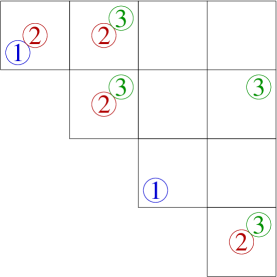
Figure 1: Initial position of the game for permutations 21435, 32154, 24153.

From the initial position the player performs a sequence of splittings, which change the set of regions, and moves, which change the arrangement of tokens.

3.2.3 Splitting

Before each move, the player subdivides the regions $R\in\mathcal{R}$, according to the following rules.

Definition 3.3.

Let $A=\{S_{\alpha}\ |\ \alpha\in I\}$ be a subset of the squares. Call $A$ an ideal subset if $I$ is closed under raising operations, i.e. If $\alpha\in I$, then $\alpha^{\prime}\in I$, whenever $\alpha^{\prime}$, and $\alpha^{\prime}-\alpha$ are both positive roots. (Equivalently, $A$ is a an ideal subset if and only if $\{e_{\alpha}\ |\ \alpha\in I\}$ span an ideal in the Lie algebra $\mathfrak{n}^{\prime}$.)

For any ideal subset $A$, we define the operation of splitting along $A$, as follows: we subdivide each region $R$ into two regions $R\cap A$ and $R\cap A^{c}$. (Empty regions produced in this way can be ignored.) Thus $\mathcal{R}$ is replaced by

$$\mathcal{R}^{\prime}=\{R_{1}\cap A,R_{1}\cap A^{c},\,R_{2}\cap A,R_{2}\cap A^{c},\,\ldots,\,R_{r}\cap A,R_{r}\cap A^{c}\}.$$

In principle the player may split along any arbitrary collection of ideal subsets between moves; however, this is inadvisable. The player should split along an ideal subset $A$ if and only if the total number of tokens in the squares of $A$ is exactly equal to $\#(A)$. If this condition is followed, each new region will always have the property that the number of tokens within the region is equal to the number of squares in the region. When splitting is performed with every $A$ satisfying this condition, we call the process splitting maximally. No choice is involved in splitting maximally.

3.2.4 Moving

After the regions have been split maximally, the player makes a move. A move is specified by a triple $[k,\beta,R]$, where $k\in\{1,\ldots,s\}$ is a choice of token label, $\beta\in\Delta^{\prime}_{+}$, and $R\in\mathcal{R}$ is a choice of region.

To execute the move $[k,\beta,R]$ we change the arrangement of tokens as follows. Find all pairs of squares $S_{\alpha},S_{\alpha}^{\prime}\in R$ such that $\alpha^{\prime}-\alpha=\beta$, and proceeding in order of decreasing height of $\alpha$, if a $k$-token occurs in the square $S_{\alpha}$ but not in $S_{\alpha^{\prime}}$, move it from the first square to the second square.

Using Definition 2.4 the result of a move can be described as follows. If $\mathcal{T}^{\prime}_{1},\ldots,\mathcal{T}^{\prime}_{s}$ represents the arrangement of tokens after the move $[k,\beta,R]$, then for any region $R^{\prime}\in\mathcal{R}$,

$$\mathcal{T}^{\prime}_{j}\cap R^{\prime}=\begin{cases}\mathcal{T}_{j}\cap R^{\prime},&\text{if $R^{\prime}\neq R$ or $j\neq k$}\\ (\mathcal{T}_{k}\cap R)\boxplus_{R}\beta&\text{otherwise.}\end{cases}$$

3.2.5 Play of the game

Beginning with the initial position, the player alternates between splitting maximally (to subdivide the regions), and making a move to change the arrangement of tokens.

Definition 3.4.

The game is won if at any point there is exactly one token in each square.

Observe that a token can only ever move from a square $S_{\alpha}$ to $S_{\alpha^{\prime}}$, where $\alpha^{\prime}$ is a higher root than $\alpha$. So, for example, if there are two tokens in the square corresponding to the highest root, there is no point in proceeding further. More generally, the game is lost if there is an ideal subset $A$ such that the the total number of tokens in $A$ is more than $\#(A)$.

An important special case is when the initial configuration of tokens is a losing position. An example of this is shown in Figure 2.

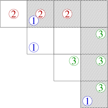
Figure 2: The initial position for permutations 23154, 41235, 13542 is a losing position, as there are there are 7 tokens in the 6 shaded squares.

Definition 3.5.

If the game is lost before the first move is made, we say the game is doomed.

Note that, while a doomed game cannot be won, it is not the case that all games which cannot be won are doomed (as seen in Section 3.4.2).

3.2.6 Vanishing and non-vanishing criteria

From games which are doomed, and games which can be won, we obtain vanishing and non-vanishing criteria respectively.

Theorem 1.

If the root game corresponding to $(\pi_{1},\ldots,\pi_{s})$ is doomed, then $c_{\pi_{1}\ldots\pi_{s}}=0$.

Theorem 2.

If the root game corresponding to $(\pi_{1},\ldots,\pi_{s})$ can be won, then $c_{\pi_{1}\ldots\pi_{s}}\geq 1$.

Remark 3.6.

It is also possible to play the game, omitting the splitting stage. This simplifies the combinatorics considerably, and Theorem 2 still holds. However, as mentioned already, it is always advisable to split maximally between moves. It is easy to show that if the game can be won by omitting the splitting step, it can be still be won while including it (c.f. Section 3.5.1).

Remark 3.7.

In the case where the game is doomed as a result of an ideal subset $A$ which is maximal (i.e. $A$ consists of all squares except for a single $S_{\alpha}$, where $\alpha$ is a simple root), Theorem 1 reduces to the DC-triviality vanishing condition in [Kn].

Theorems 1 and 2 cast a large net over the set of all Schubert problems, and capture a huge number of them. It is not hard to see, for instance, that the probability of finding a non-doomed game at random for $SL(n)$ tends to $0$ as $n\to\infty$. Still there is a small gap: in general, not being able to win the game does not provide any information. However, in a number special cases, we have been able to show that the converse of Theorem 2 holds. These are discussed in Section 3.5.

3.3 Relating the combinatorics and geometry

Given an arrangement of tokens, $\mathcal{T}_{1},\ldots,\mathcal{T}_{s}$, and a region $R\in\mathcal{R}$, we associate the following linear spaces.

• A $B^{\prime}$-module $V^{\prime}$, a subquotient of $\mathfrak{n}^{\prime}$, such that $R$ is the set of distinct $T^{\prime}$-weights of $V^{\prime}$.

• For each $i=1,\ldots,s$, a linear subspace $U_{i}\subset V^{\prime}$ such that $\mathcal{T}_{i}\cap R$ is the set of $T^{\prime}$ weights of $U_{i}$.

Put $V=V^{\prime}\oplus\cdots\oplus V^{\prime}$ ($s$-summands), and $U=U_{1}\oplus\cdots\oplus U_{s}\subset V$. We have a $B^{\prime}$-equivariant map $\phi:V\to V^{\prime}$ given by $\phi(v_{1},\ldots,v_{s})=v_{1}+\cdots+v_{s}$. Thus we have a quadruple $(U,V,V^{\prime},\phi)$, as in Section 2.6.

At any position in the game, there is one such quadruple for every region. Recall the notion of a good quadruple from Section 2.6. In our current context, the quadruple $(U,V,V^{\prime},\phi)$ is good if and only if there exist $a_{1},\ldots,a_{s}\in N$ such that $a_{1}\cdot U_{1}\oplus\cdots\oplus a_{s}\cdot U_{s}=V^{\prime}$. A position is a winning position if and only if $U_{1}\oplus\cdots\oplus U_{s}=V^{\prime}$ for every region. In particular, the quadruples associate to winning positions are good.

To prove Theorem 2, we show that if the quadruple associated to every region is good, then the quadruple associated to initial position is good. This is true essentially because the moves and splittings combinatorially encode the geometric ideas in Propositions 2.7 and 2.9. A move in the root game changes $U$ (for a single region) to a new subspace $U^{1}\subset V^{\prime}$ in exactly the manner prescribed by Proposition 2.7. Thus, if the new quadruple $(U^{1},V,V^{\prime},\phi)$ is good, then old quadruple $(U,V,V^{\prime},\phi)$ must be good too. Similarly a splitting changes the set of quadruples following Proposition 2.9. Hence from a winning position (where all regions correspond to good quadruples), we can backtrack all the way to the start the game and deduce that the initial position is good.

Now, the statement that the initial position is good is precisely condition 2 of Corollary 2.5. Thus, by Corollary 2.5, the initial position is good if and only if $c_{\pi_{1}\ldots\pi_{s}}\neq 0$.

Many of the details have been omitted here. A more precise account of relationship between the geometry and combinatorics is given in the proofs in Section 4.5.

3.4 Examples

3.4.1 Games which can be won

In type $A$, for any fixed $\beta=\alpha_{ij}$, the possible squares involved in a move corresponding to $\beta$ are $\{S_{\alpha_{kl}}\ |\ \text{$k=i$ or $l=i$}\}\cup\{S_{\alpha_{kl}}\ |\ \text{$k=j$ or $l=j$}\}$. These squares lie on two reflected lines which meet at the square $S_{\beta}$ (shown as dotted lines in Figures 3 and 4). The tokens move strictly horizontally or vertically from one reflected line the other.

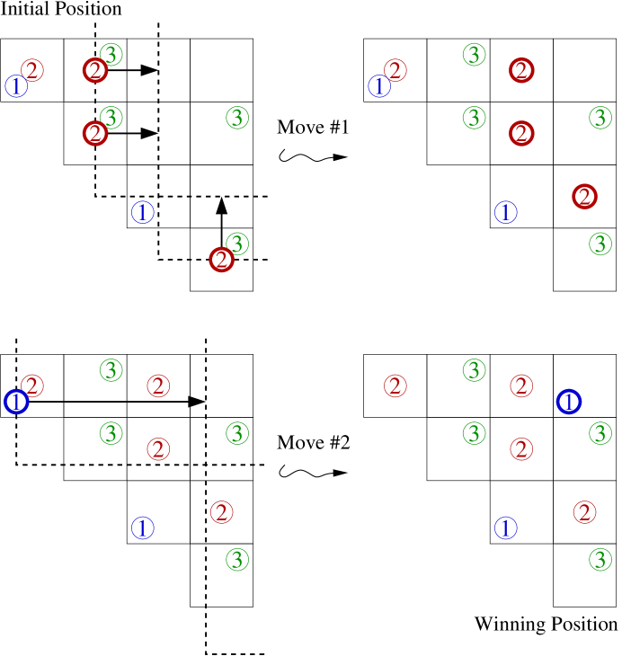
Figure 3: Moves $[2,\alpha_{34}]$ and $[1,\alpha_{25}]$ are applied to the initial position in Figure 1.

Figure 3 shows a sequence of moves in a game which has been played without the splitting step, to better illustrate the movement of the tokens. The initial position is $(21435,32154,24153)$, from Figure 1. The sequence of moves leads to a winning position.

Figure 4 gives an example of a sequence of moves with maximal splitting in between moves. Again the sequence of moves leads to a winning position.

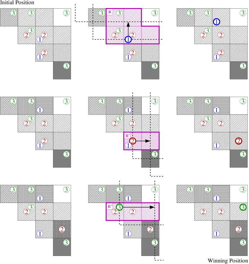
Figure 4: The general game, played out for permutations 13425, 41325, 14352. The moves, shown in the centre column, are: $[1,\alpha_{12},R]$, $[2,\alpha_{45},R^{\prime}]$, and finally $[3,\alpha_{35},R^{\prime\prime}]$. The left column shows the state before the move, in which the set of squares is maximally divided into regions. The right column shows the state immediately after the move, before further subdividing.

3.4.2 Converses and counterexamples

The converse of Theorem 1 is certainly not true. The first counterexamples in $SL(n)$ occur for $n=4$. See Figure 5.

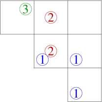
Figure 5: The permutations $\pi_{1}=1432$, $\pi_{2}=2314$, $\pi_{3}=2134$ are a counterexample to the converse of Theorem 1. The game is not doomed, though $c_{\pi_{1}\pi_{2}\pi_{3}}=0$. All other $SL(4)$ counterexamples are similar to this one.

If the root game is played without splitting, the converse of Theorem 2 is not true. The first counterexamples in $SL(n)$ occur for $n=5$. Figure 6 shows the initial position of the game for the permutations 23145, 14253, 41523. There is only one square with 2 tokens, and one empty square. Without splitting, any effort to rectify this imbalance winds up moving more than just one token. However, with splitting, the game can be won.

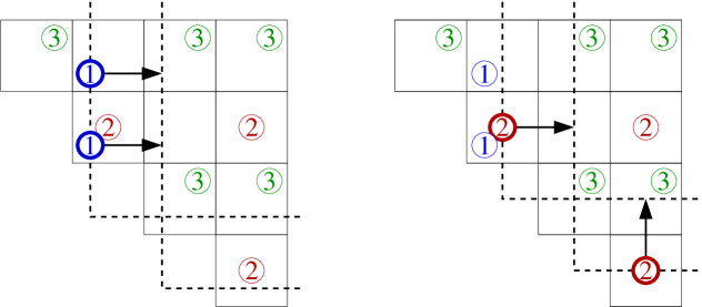
Figure 6: The permutations 23145, 14253, 41523 give a counterexample to the converse of Theorem 2, if the game is played without splitting. If we split maximally first, either of the moves shown (restricted to the appropriate region) will win the game.

3.4.3 Other types

We now describe a ‘sensible’ way to arrange the squares in types $B$ and $D$ ($G^{\prime}=SO(n)$). A similar arrangement to the type $B$ arrangement can be used for type $C$ ($G^{\prime}=Sp(2n)$).

In both examples $x_{1},\ldots,x_{n}$ is an orthonormal basis for $\mathbb{R}^{n}$.

Example 3.8.

If $G^{\prime}=SO(2n)$, the root system $\Delta^{\prime}=D_{n}$ is

$$\{(-1)^{\varepsilon}x_{i}+(-1)^{\delta}x_{j}\ |\ i\neq j\}.$$

The positive roots are of two types:

$$\{\beta{ij}=x_{j}-x_{i}\ |\ i<j\}\cup\{\beta^{\prime}_{ij}=x_{j}+x_{i}\ |\ i<j\}$$

We arrange these the squares inside a $2n\times n$ array (denoted $DS_{ij}$) as follows: the root $\beta_{ij}$ corresponds to the square $DS_{n+i,j}$; the root $\beta^{\prime}_{ij}$ corresponds to the square $DS_{n+1-i,j}$.

$$\Delta(SO(10))_{+}=(D_{5})_{+}=\text{ \begin{tabular}[]{cccc}\cline{4-4}\cr&&&\vrule\lx@intercol\hfil\rule[-8.0pt]{0.0pt}{24.0pt}$\beta^{\prime}_{45}$\hfil\lx@intercol\vrule\lx@intercol \\ \cline{3-4}\cr&&\vrule\lx@intercol\hfil\rule[-8.0pt]{0.0pt}{24.0pt}$\beta^{\prime}_{34}$\hfil\lx@intercol &\vrule\lx@intercol\hfil\rule[-8.0pt]{0.0pt}{24.0pt}$\beta^{\prime}_{35}$\hfil\lx@intercol\vrule\lx@intercol \\ \cline{2-4}\cr&\vrule\lx@intercol\hfil\rule[-8.0pt]{0.0pt}{24.0pt}$\beta^{\prime}_{23}$\hfil\lx@intercol &\vrule\lx@intercol\hfil\rule[-8.0pt]{0.0pt}{24.0pt}$\beta^{\prime}_{24}$\hfil\lx@intercol &\vrule\lx@intercol\hfil\rule[-8.0pt]{0.0pt}{24.0pt}$\beta^{\prime}_{25}$\hfil\lx@intercol\vrule\lx@intercol \\ \hline\cr\vrule\lx@intercol\hfil\rule[-8.0pt]{0.0pt}{24.0pt}$\beta^{\prime}_{12}$\hfil\lx@intercol &\vrule\lx@intercol\hfil\rule[-8.0pt]{0.0pt}{24.0pt}$\beta^{\prime}_{13}$\hfil\lx@intercol &\vrule\lx@intercol\hfil\rule[-8.0pt]{0.0pt}{24.0pt}$\beta^{\prime}_{14}$\hfil\lx@intercol &\vrule\lx@intercol\hfil\rule[-8.0pt]{0.0pt}{24.0pt}$\beta^{\prime}_{15}$\hfil\lx@intercol\vrule\lx@intercol \\ \hline\cr\vrule\lx@intercol\hfil\rule[-8.0pt]{0.0pt}{24.0pt}$\beta_{12}$\hfil\lx@intercol &\vrule\lx@intercol\hfil\rule[-8.0pt]{0.0pt}{24.0pt}$\beta_{13}$\hfil\lx@intercol &\vrule\lx@intercol\hfil\rule[-8.0pt]{0.0pt}{24.0pt}$\beta_{14}$\hfil\lx@intercol &\vrule\lx@intercol\hfil\rule[-8.0pt]{0.0pt}{24.0pt}$\beta_{15}$\hfil\lx@intercol\vrule\lx@intercol \\ \hline\cr&\vrule\lx@intercol\hfil\rule[-8.0pt]{0.0pt}{24.0pt}$\beta_{23}$\hfil\lx@intercol &\vrule\lx@intercol\hfil\rule[-8.0pt]{0.0pt}{24.0pt}$\beta_{24}$\hfil\lx@intercol &\vrule\lx@intercol\hfil\rule[-8.0pt]{0.0pt}{24.0pt}$\beta_{25}$\hfil\lx@intercol\vrule\lx@intercol \\ \cline{2-4}\cr&&\vrule\lx@intercol\hfil\rule[-8.0pt]{0.0pt}{24.0pt}$\beta_{34}$\hfil\lx@intercol &\vrule\lx@intercol\hfil\rule[-8.0pt]{0.0pt}{24.0pt}$\beta_{35}$\hfil\lx@intercol\vrule\lx@intercol \\ \cline{3-4}\cr&&&\vrule\lx@intercol\hfil\rule[-8.0pt]{0.0pt}{24.0pt}$\beta_{45}$\hfil\lx@intercol\vrule\lx@intercol \\ \cline{4-4}\cr\end{tabular} }$$

Example 3.9.

If $G^{\prime}=SO(2n+1)$, the root system $\Delta^{\prime}=B_{n}$ is

$$\{(-1)^{\varepsilon}x_{i}+(-1)^{\delta}x_{j}\ |\ i\neq j\}\cup\{\pm x_{i}\}.$$

The positive roots are of three types:

$$\Delta^{\prime}_{+}=\{\gamma_{ij}=x_{j}-x_{i}\ |\ i<j\}\cup\{\gamma^{\prime}_{ij}=x_{j}+x_{i}\ |\ i<j\}\cup\{\gamma^{\circ}_{j}=x_{j}\}.$$

We arrange the squares inside a $(2n+1)\times n$ array of squares (denoted $BS_{ij}$) as follows: the root $\gamma_{ij}$ corresponds to the square $BS_{n+1+i,j}$; the root $\gamma^{\prime}_{ij}$ corresponds to the square $BS_{n+1-i,j}$; the root $\gamma^{\circ}_{j}$ corresponds to the square $BS_{n+1,j}$.

$$\Delta(SO(9))_{+}=(B_{4})_{+}=\text{ \begin{tabular}[]{cccc}\cline{4-4}\cr&&&\vrule\lx@intercol\hfil\rule[-8.0pt]{0.0pt}{24.0pt}$\gamma^{\prime}_{34}$\hfil\lx@intercol\vrule\lx@intercol \\ \cline{3-4}\cr&&\vrule\lx@intercol\hfil\rule[-8.0pt]{0.0pt}{24.0pt}$\gamma^{\prime}_{23}$\hfil\lx@intercol &\vrule\lx@intercol\hfil\rule[-8.0pt]{0.0pt}{24.0pt}$\gamma^{\prime}_{24}$\hfil\lx@intercol\vrule\lx@intercol \\ \cline{2-4}\cr&\vrule\lx@intercol\hfil\rule[-8.0pt]{0.0pt}{24.0pt}$\gamma^{\prime}_{12}$\hfil\lx@intercol &\vrule\lx@intercol\hfil\rule[-8.0pt]{0.0pt}{24.0pt}$\gamma^{\prime}_{13}$\hfil\lx@intercol &\vrule\lx@intercol\hfil\rule[-8.0pt]{0.0pt}{24.0pt}$\gamma^{\prime}_{14}$\hfil\lx@intercol\vrule\lx@intercol \\ \hline\cr\vrule\lx@intercol\hfil\rule[-8.0pt]{0.0pt}{24.0pt}$\gamma^{\circ}_{1}$\hfil\lx@intercol &\vrule\lx@intercol\hfil\rule[-8.0pt]{0.0pt}{24.0pt}$\gamma^{\circ}_{2}$\hfil\lx@intercol &\vrule\lx@intercol\hfil\rule[-8.0pt]{0.0pt}{24.0pt}$\gamma^{\circ}_{3}$\hfil\lx@intercol &\vrule\lx@intercol\hfil\rule[-8.0pt]{0.0pt}{24.0pt}$\gamma^{\circ}_{4}$\hfil\lx@intercol\vrule\lx@intercol \\ \hline\cr&\vrule\lx@intercol\hfil\rule[-8.0pt]{0.0pt}{24.0pt}$\gamma_{12}$\hfil\lx@intercol &\vrule\lx@intercol\hfil\rule[-8.0pt]{0.0pt}{24.0pt}$\gamma_{13}$\hfil\lx@intercol &\vrule\lx@intercol\hfil\rule[-8.0pt]{0.0pt}{24.0pt}$\gamma_{14}$\hfil\lx@intercol\vrule\lx@intercol \\ \cline{2-4}\cr&&\vrule\lx@intercol\hfil\rule[-8.0pt]{0.0pt}{24.0pt}$\gamma_{23}$\hfil\lx@intercol &\vrule\lx@intercol\hfil\rule[-8.0pt]{0.0pt}{24.0pt}$\gamma_{24}$\hfil\lx@intercol\vrule\lx@intercol \\ \cline{3-4}\cr&&&\vrule\lx@intercol\hfil\rule[-8.0pt]{0.0pt}{24.0pt}$\gamma_{34}$\hfil\lx@intercol\vrule\lx@intercol \\ \cline{4-4}\cr\end{tabular} }$$

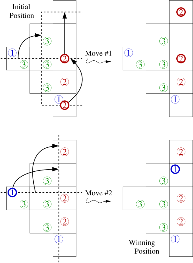
Figure 7: A simple game for $SO(7,\mathbb{C})$. In this example, $\pi_{1}=\bar{1}32$, $\pi_{2}=231$, $\pi_{3}=\bar{1}\bar{2}3$. The root $\beta$ which is used in each move is the crossing point of the dotted lines.

Figure 7 gives an example of a root game for $SO(7,\mathbb{C})$. Here, an element of Weyl group $W=C_{2}^{3}\rtimes S_{3}$ can be represented by a permutation $a_{1}a_{2}a_{3}$ of $123$, where each symbol is either decorated with a bar or not. This permutation acts on $\mathbb{R}^{3}$ by the matrix whose $i^{th}$ row is $x_{a_{i}}$ if $i$ is unbarred, and $-x_{a_{i}}$ if $i$ is barred.

Arrows in Figure 7 are included not only for all tokens that move, but for all pairs of roots $\alpha,\alpha^{\prime}$, whose difference is $\beta$. Since the game can be won using the moves shown, for $\pi_{1}=\bar{1}32$, $\pi_{2}=231$, $\pi_{3}=\bar{1}\bar{2}3$ we have $c_{\pi_{1}\pi_{2}\pi_{3}}\geq 1$.

3.5 Remarks

3.5.1 Splitting

In the rules of the root game, we are told exactly when to split regions: we split along an ideal subset $A$ if and only if the number of tokens in $A$ equals $\#(A)$. However, it turns out that this condition is never used in the proof. Thus, in theory, the rules could be relaxed so that the player has the option to split regions along any ideal subset $A$ between moves. That said, we will now sketch a proof that it is never advantageous to the player to exercise this freedom.

Suppose the rules tell us not to split along $A$. If we do split along $A$ there will be too many tokens in one region. Since regions can never be rejoined once they are split, the game cannot be won. On the other hand, suppose the rules tell us to split along $A$, and the player chooses not to. Of any move that is made subsequently, one of the following two things must be true: either the same arrangement of tokens could have been reached (possibly using multiple moves) if we had split along $A$, or the move caused the game to be lost.

The ability to determine, a priori when splitting is advantageous, relies on the fact that we have assumed $\sum_{i=1}^{s}\ell(\pi_{i})=\dim G^{\prime}/B^{\prime}$.

3.5.2 Products which are not top degree

The root game can be adapted to analyse the non-vanishing of a product of Schubert classes, whether or not the product is not of top degree. This greater generality is handled by the root game for branching Schubert calculus, so we will not discuss it at length. However only two minor modifications to the rules are required. First, we must change the winning condition to read “the game is won if there is at most one token in each square”, rather than “… exactly one token in each square”. (The losing and doomed conditions remain as stated previously.) Second, we must remove the rule forcing us to split maximally between moves, and instead have splitting be at the player’s discretion, as discussed in Section 3.5.1.

3.5.3 Relationship with the Bruhat order

For products of only two Schubert classes, the converse of Theorem 2 holds: being able to win the root game both necessary and sufficient for non-vanishing. In this case, the non-vanishing of the product is determined precisely by the Bruhat order. That is, $\omega_{\pi_{1}}\cdot\omega_{\pi_{2}}\neq 0$ if and only if $\pi_{1}\leq w_{0}\pi_{2}$ in the Bruhat order.

In the case where the product is top degree, i.e. $\ell(\pi_{1})+\ell(\pi_{2})=\dim G/B$, the fact that we can win the root game is a triviality: we have $\pi_{1}\leq w_{0}\pi_{2}$ if and only if $\pi_{1}=w_{0}\pi_{2}$, in which case the set of squares containing a $1$-token is the complement of the set of squares containing a $2$-token. Thus the initial position of the game is already a winning position.

Less trivial is the case when $\pi_{1}<w_{0}\pi_{2}$. Since the product of the classes is not top degree, we must use the revised notion of winning position (see Section 3.5.2). Nevertheless, we have the following theorem.

Theorem 3.

$\omega_{\pi_{1}}\cdot\omega_{\pi_{2}}\neq 0$ if and only if it is possible to win the root game corresponding to $(\pi_{1},\pi_{2})$.

A detailed proof of this result is given in the author’s doctoral thesis [P2].

3.5.4 Converses and computations

It would be quite surprising and remarkable if the converse of Theorem 2 were true in any generality. So far, for $SL(n)$, the converse has deftly eluded any counterexamples. In fact the converse of Theorem 2 has been affirmed by an exhaustive computer search for $SL(n)$ for $n\leq 7$. The converse of Theorem 2 (with $s=3$) has also been verified for the exceptional group $G_{2}$, as well as for $SO(5)$ and $SO(7)$. (The next smallest exceptional group, $F_{4}$, is unfortunately beyond our computational abilities at the moment.)

One special case where the converse of Theorem 2 is true is when the classes $\omega_{\pi_{i}}$ are pulled back from a Grassmannian in an appropriate way. We prove this result in [P1]. Another special case is Theorem 3, which tells us that the converse is true for products of only two Schubert classes.

For the groups $SO(n)$, $n\geq 8$, the converse of Theorem 2 is in fact false. For $SO(8)$, we represent an element of the Weyl group $W=C_{2}^{3}\rtimes S_{4}$ by a permutation $a_{1}a_{2}a_{3}a_{4}$ of $0123$, where each symbol, except $0$, is either decorated with a bar or not ($0$ is always unbarred). This permutation acts on $\mathbb{R}^{4}$ by the matrix whose $i^{th}$ row is $x_{a_{i}}$ if $i$ is unbarred, and $-x_{a_{i}}$ if $i$ is barred. The two counterexamples to the converse of Theorem 2 for $SO(8)$ are listed below.

$\pi_{1}$	$\pi_{2}$	$\pi_{3}$
$0\bar{1}32$	$0\bar{2}31$	$03\bar{2}1$
$03\bar{1}2$	$0\bar{2}31$	$0\bar{2}31$

The problem that arises in these examples is that although there exists a $T$-fixed point $(U_{1},U_{2},U_{3})$ on $Gr(V^{\prime})^{3}$ with $U_{1}\oplus U_{2}\oplus U_{3}=V^{\prime}$, which is a degeneration of $(a_{1}\cdot P_{1},a_{2}\cdot P_{2},a_{3}\cdot P_{3})$, the moves of the game fail to find it. We are not aware of any examples in which $c_{\pi_{1}\ldots\pi_{s}}\geq 1$ but where there are no suitable $T$-fixed points on any of the relevant varieties. It therefore seems it would be desirable to be able to describe a larger set of moves—moves which, starting from a $T$-fixed point on $Gr(V^{\prime})^{s}$ can reach all the other $T$-fixed points in its $(N^{\prime})^{s}$-orbit closure.

With $s=3$, a restriction one might wish to make to the root game is to allow only moves involving tokens labeled $1$ and $2$. This restriction seems appropriate when viewing Schubert calculus as taking products in cohomology rather than intersection numbers. Under this weakening, Theorem 2 remains true (obviously), but the converse is already false for $SL(n)$. There are no examples of this for $n\leq 5$; however, for $n=6$ there are a total of four such examples:

$\pi_{1}$	$\pi_{2}$	$\pi_{3}$
145326	321564	315264
154326	312564	315264
514326	152364	135264
154236	312654	315264

It is possible dispose of these $SL(6)$ counterexamples, by introducing new moves geometrically based on Proposition 2.10. One such move (called a merge) is the following: select a region $R$, and a pair of token labels: $k_{1}\neq k_{2}$, with the property that there is no square in $R$ which contains both a $k_{1}$-token and a $k_{2}$-token. Then replace every $k_{2}$-token with a $k_{1}$-token in the same square. If we introduce merges into the root game, the aforementioned counterexamples disappear. Moreover, it follows (though we omit the proof here) that the converse of Theorem 2 (with merges included) is true for $SL(6)$ for any $s$.

4 Root games for branching Schubert calculus

We now describe the root game for the more general branching problem. We will see that although the setup is slightly different, this game specialises to the root game for vanishing of Schubert intersection numbers.

The main differences we shall see are the following:

1. Squares correspond to positive roots of $G$ rather than $G^{\prime}$.

2. Tokens do not have labels.

3. The winning condition is defined in terms of the map $\hat{\phi}:\Delta_{+}\to\Delta^{\prime}_{+}\cup\{0\}$ (which we calculate explicitly in a number of examples).

4. Splitting is more complicated—it also involves $\hat{\phi}$.

4.1 The map $\hat{\phi}$

Recall the definition of the map $\hat{\phi}$ from Section 2.1. The rules of the game heavily involve $\hat{\phi}$; thus before proceeding further, we compute this map in a number of important examples.

Example 4.1.

If $G^{\prime}\hookrightarrow G_{1},\ldots,G^{\prime}\hookrightarrow G_{s}$, then $G^{\prime}\hookrightarrow G=G_{1}\times\cdots\times G_{s}$ via the diagonal map. Let $\hat{\phi}_{i}:\Delta(G_{i})_{+}\to\Delta^{\prime}\cup\{0\}$ denote the map on root systems for $G^{\prime}\hookrightarrow G_{i}$. The positive roots of $G$ are $\Delta_{+}=\Delta(G_{1})_{+}\sqcup\dots\sqcup\Delta(G_{s})_{+}$, and

$$\hat{\phi}:\Delta_{+}\to\Delta^{\prime}_{+}\cup\{0\}$$

is simply given by $\hat{\phi}(\alpha)=\phi_{i}(\alpha)$ if $\alpha\in\Delta(G_{i})_{+}$.

In particular, if $G^{\prime}=G_{1}=\cdots=G_{s}$, then each $\hat{\phi}_{i}$ is just the identity map. Thus this example allows us to deal with the vanishing problem for multiplication of Schubert calculus.

Example 4.2.

If $G^{\prime}=SL(k)\hookrightarrow G=SL(n)$ is the inclusion

$$A\mapsto\left(\begin{matrix}A&0\\ 0&I_{n-k}\end{matrix}\right)$$

then

$$\hat{\phi}(\alpha_{ij})=\begin{cases}\alpha_{ij}\in\Delta^{\prime},&\text{if $j\leq k$}\\ 0,&\text{otherwise}\end{cases}$$

In this example $i^{*}$ is easily described as an operation on Schubert polynomials [LS]. If $\omega_{\pi}$ is represented by a Schubert polynomial in variables $x_{1},\ldots,x_{n}$ then $i^{*}(\omega_{\pi})$ is given by setting $x_{k+1}=\cdots=x_{n}=0$.

We now consider the inclusion of $SO(n,\mathbb{C})\hookrightarrow G=SL(n)$. We begin with the case where $n$ is even. Let $R$ denote the $n/2\times n/2$ matrix with $1$ on the antidiagonal, and $0$ everywhere else. We take as a (compact) maximal torus of $SO(n,\mathbb{R})$ the subgroup

$$T^{\prime}_{\mathbb{R}}=\big{\{}\left(\begin{matrix}A&BR\\ -RB&RAR\end{matrix}\right)\in GL(n,\mathbb{R})\ \big{|}\ \text{$A$, $B$ are diagonal}\}.$$

The complexification $T^{\prime}$ of $T^{\prime}_{\mathbb{R}}$ is a complex maximal torus in $SO(n,\mathbb{C})$.

Since the standard maximal torus of $SO(n)$ is not a subgroup of the standard (diagonal) maximal torus of $SL(n)$, we use a suitable conjugate subgroup of $SO(n)$. Let

$$U=\left(\begin{matrix}I&iR\\ iR&I\end{matrix}\right).$$

$\beta_{34}$	$\beta_{24}$	$\beta_{14}$	$\beta^{\prime}_{14}$	$\beta^{\prime}_{24}$	$\beta^{\prime}_{34}$
	$\beta_{23}$	$\beta_{13}$	$\beta^{\prime}_{13}$	$\beta^{\prime}_{23}$		$\beta^{\prime}_{34}$
		$\beta_{12}$	$\beta^{\prime}_{12}$		$\beta^{\prime}_{23}$	$\beta^{\prime}_{24}$
				$\beta^{\prime}_{12}$	$\beta^{\prime}_{13}$	$\beta^{\prime}_{14}$
				$\beta_{12}$	$\beta_{13}$	$\beta_{14}$
					$\beta_{23}$	$\beta_{24}$
						$\beta_{34}$

Figure 8: The map $\hat{\phi}:\Delta(SL(8))_{+}\to\Delta(SO(8))_{+}\cup\{0\}$. The root $\hat{\phi}(\alpha)$ is written in the square corresponding to $\alpha$. Empty squares are mapped to $0$.

Example 4.3.

Let $G^{\prime}=U\,SO(n)\,U^{-1}\hookrightarrow G=SL(n)$, where $n=2m$. One can easily verify that a maximal torus of $G^{\prime}$, is the set of invertible diagonal matrices

$$U\,T^{\prime}\,U^{-1}=\big{\{}\lambda=\left(\begin{matrix}\lambda_{m}&&&&&\\ &\ddots&&&&\\ &&\lambda_{1}&&&\\ &&&\lambda_{1}^{-1}&&\\ &&&&\ddots&\\ &&&&&\lambda_{m}^{-1}\end{matrix}\right)\in SL(n)\big{\}}.$$

The Lie algebra $\mathfrak{g}^{\prime}=\{(a_{ij})\in\mathfrak{sl}(n)\ |\ a_{ij}=-a_{n+1-i\ j}\}$, is the set of $n\times n$ matrices which are skew symmetric about the antidiagonal. And $\mathfrak{n}^{\prime}$ is simply the set of upper triangular matrices in $\mathfrak{g}^{\prime}$.

Let $E_{ij}$ denote the matrix with a $1$ in the $i,j$ position, and $0$ everywhere else. We see that for $i<j$,

$$\lambda E_{ij}\lambda^{-1}=\begin{cases}\lambda_{m+1-i}\lambda_{j-m}E_{ij},&\text{if $i+j>n+1$, $i\leq m$}\\ \lambda_{m+1-i}\lambda_{j-m}E_{ij},&\text{if $i+j\leq n$, $j>m$}\\ \lambda_{m+1-i}\lambda_{m+1-j}^{-1}E_{ij},&\text{if $j\leq m$}\\ \lambda_{i-m}^{-1}\lambda_{j-m}E_{ij},&\text{if $i>m$}\\ 0,&\text{if $i+j=n+1$}\\ \end{cases}$$

Thus $\hat{\phi}$ is given by

$$\hat{\phi}(\alpha_{ij})=\begin{cases}\beta^{\prime}_{{m+1-i},{j-m}},&\text{if $i+j>n+1$, $i\leq m$}\\ \beta^{\prime}_{{j-m},{m+1-i}},&\text{if $i+j\leq n$, $j>m$}\\ \beta_{{m+1-j},{m+1-i}},&\text{if $j\leq m$}\\ \beta_{{i-m},{j-m}},&\text{if $i>m$}\\ 0,&\text{if $i+j=n+1$}\\ \end{cases}$$

In terms of the arrangement of squares (described in Examples 3.1 and 3.8), the map $\hat{\phi}$ is symmetrical about the antidiagonal, with the antidiagonal itself mapping to $0$. Moreover, below the antidiagonal (i.e. for $i+j>n+1$), we simply have $\hat{\phi}(AS_{ij})=DS_{i-m,j}$. See Figure 8.

The analysis for $n$ odd is very similar.

Example 4.4.

Let $G^{\prime}\hookrightarrow G=SL(n)$, where $n=2m-1$ and $G^{\prime}$ is an appropriately chosen conjugate of $SO(n)$.

As in the case where $n$ is even, $\mathfrak{g}^{\prime}=\{(a_{ij})\in\mathfrak{sl}(n)\ |\ a_{ij}=-a_{n+1-i,j}$, is the set of $n\times n$ matrices which are skew symmetric about the antidiagonal, and $\mathfrak{n}^{\prime}=\mathfrak{b}\cap\mathfrak{g}^{\prime}$. The map $\hat{\phi}$ is given by

$$\hat{\phi}(\alpha_{ij})=\begin{cases}\gamma^{\circ}_{i},&\text{if $j=m$}\\ \gamma^{\circ}_{j},&\text{if $i=m$}\\ \gamma^{\prime}_{{m-i},{j-m}},&\text{if $i+j>n+1$, $i<m$}\\ \gamma^{\prime}_{{j-m},{m-i}},&\text{if $i+j\leq n$, $j>m$}\\ \gamma_{{m-j},{m-i}},&\text{if $j<m$}\\ \gamma_{{i-m},{j-m}},&\text{if $i>m$}\\ 0,&\text{if $i+j=n+1$}\\ \end{cases}$$

More simply, in terms of the arrangement of squares (see Examples 3.1 and 3.9), we have that $\hat{\phi}$ is symmetrical about the antidiagonal, and identically zero on the antidiagonal. Below the antidiagonal $\hat{\phi}(AS_{ij})=BS_{i,j-m}$. See Figure 9.

$\gamma_{23}$	$\gamma_{13}$	$\gamma^{\circ}_{3}$	$\gamma^{\prime}_{13}$	$\gamma^{\prime}_{23}$
	$\gamma_{12}$	$\gamma^{\circ}_{2}$	$\gamma^{\prime}_{12}$		$\gamma^{\prime}_{23}$
		$\gamma^{\circ}_{2}$		$\gamma^{\prime}_{12}$	$\gamma^{\prime}_{13}$
			$\gamma^{\circ}_{1}$	$\gamma^{\circ}_{2}$	$\gamma^{\circ}_{3}$
				$\gamma_{12}$	$\gamma_{13}$
					$\gamma_{23}$

Figure 9: The map $\hat{\phi}:\Delta(SL(7))_{+}\to\Delta(SO(7))_{+}\cup\{0\}$. The root $\hat{\phi}(\alpha)$ is written in the square corresponding to $\alpha$. Empty squares are mapped to $0$.

Example 4.5.

Let $G$ be the complex form of $G_{2}$, and $G^{\prime}=SL(3)$. The map $i:G^{\prime}\hookrightarrow G$ is defined on the level of roots: $A_{2}$ includes into $G_{2}$ as the long roots. Since $SL(3)$ is simply connected, this defines a homomorphism on the Lie groups (and this map is an inclusion). The map $\hat{\phi}:(G_{2})_{+}\to(A_{2})_{+}\cup\{0\}$ is therefore

$$\hat{\phi}(\alpha)=\begin{cases}0,\qquad&\text{if $\alpha$ is a short root of $G_{2}$}\\ \alpha,\qquad&\text{if $\alpha$ is a long root of $G_{2}$.}\end{cases}$$

We arrange the squares of $G$ in a linear fashion, with the short simple root at the bottom, and the long simple root on the left. The map $\hat{\phi}$ and the arrangement of squares for $G_{2}$ are both illustrated in Figure 10.

Figure 10: The map $\hat{\phi}:(G_{2})_{+}\to(A_{2})_{+}\cup\{0\}$, and the corresponding arrangement of squares.

4.2 Rules of the game

4.2.1 Data of a position

The position in a root game consists of the following data:

• A partition of the set of positive roots of $G$, i.e. $\mathcal{R}=\{R_{1},\ldots,R_{r}\}$, such that $\Delta_{+}=\coprod_{i=1}^{s}R_{i}$. Each $R_{i}$ is called a region.

• A subset $\mathcal{T}$ of the positive roots of $G$, which we call the arrangement of tokens.

We visualise this information by drawing a square $S_{\alpha}$ for each positive root $\alpha\in\Delta_{+}$, and placing a token in $S_{\alpha}$ if $\alpha\in T$. As before, we arrange the squares in a sensible manner depending on the type of $G$ (see Examples 3.1, 3.8 and 3.9).

The regions are just sets of the squares. As such, if $R$ is a region, we will sometimes write $S_{\alpha}\in R$ rather than $\alpha\in R$.

4.2.2 Initial configuration

The game always begins with a single region ($\mathcal{R}=\{\Delta_{+}\}$), which contains all the squares. The initial arrangement of tokens is the inversion set of $\pi$, i.e.

$$\mathcal{T}=\{\alpha\in\Delta_{+}\ |\ \pi\cdot\alpha\in\Delta_{-}\}.$$

Example 4.6.

If $G=SL(5)\times SO(5)$, $\pi=(23154,r_{\gamma^{\circ}_{1}})$ where $r_{\gamma^{\circ}_{1}})$ is the reflection in the simple root $\gamma^{\circ}_{1}$. Then the initial position is as shown below:

4.2.3 Splitting

We define splitting along $A$ as in Section 3.2.3: if $A\subset\Delta_{+}$, splitting $\mathcal{R}=\{R_{1},\ldots,R_{r}\}$ along $A$ produces

$$\mathcal{R}^{\prime}=\{R_{1}\cap A,R_{1}\cap A^{c},\,R_{2}\cap A,R_{2}\cap A^{c},\,\ldots,\,R_{r}\cap A,R_{r}\cap A^{c}\}.$$

(Empty regions have no effect on the game, thus we may discard any copies of the empty set produced in this way.)

The subsets $A\subset\Delta$ which can be legally used for splitting are called splitting subsets.

Definition 4.7.

Let $A\subset\Delta_{+}$ be a subset of the positive roots of $G$. We call $A$ a splitting subset if $A$ is an ideal subset (c.f. Definition 3.3), and $\hat{\phi}(A^{c})\cap\hat{\phi}(A)\subset\{0\}$.

Example 4.8.

For $SO(n)\hookrightarrow SL(n)$, a set $A\subset\Delta_{+}$ is an ideal subset if for every square $S$ in $A$, $A$ contains all squares above and to the right of $S$. $A$ is a splitting subset if it is an ideal subset which is symmetrical about the antidiagonal.

4.2.4 Moves

A move is specified by a pair $[\beta,R]$, where $\beta\in\Delta_{+}$, and $R\in\mathcal{R}$ is a choice of region. To execute the move, we find all pairs of squares $S_{\alpha},S_{\alpha}^{\prime}\in R$ such that $\alpha^{\prime}-\alpha=\beta$. We then order the relevant $S_{\alpha}$ according to the height of the root $\alpha$. Proceeding in order of decreasing height of $\alpha$, if a token appears in the square $S_{\alpha}$ but not in $S_{\alpha^{\prime}}$, move the token up from the first square to the second square.

Equivalently, using Definition 2.4 the result of a move can be described as follows. If $\mathcal{T}^{\prime}$ represents the arrangement of tokens after the move $[\beta,R]$, then for any region $R^{\prime}\in\mathcal{R}$,

$$\mathcal{T}^{\prime}\cap R^{\prime}=\begin{cases}\mathcal{T}\cap R^{\prime},&\text{if $R^{\prime}\neq R$}\\ (\mathcal{T}\cap R)\boxplus_{R}\beta.&\text{otherwise}\end{cases}$$

4.2.5 Play of the game

Beginning with the initial configuration, the player performs a sequence of moves and splittings. Moves and splittings may be performed in any order. Splitting along $A$ is permissible whenever $A$ is a splitting subset.

Definition 4.9.

The game is won if the arrangement of tokens $\mathcal{T}$ is injective (c.f. Definition 2.1).

Remark 4.10.

Splitting along $A$ is permissible whenever $A$ is a splitting subset. However, when $\ell(\pi)=\dim G^{\prime}/B^{\prime}$, one can determine a priori whether splitting will help us win the root game. It turns out that if $\ell(\pi)=\dim G^{\prime}/B^{\prime}$, the splitting is advantageous if and only if $\#(\mathcal{T}\cap A)=\#(\hat{\phi}(A)\setminus\{0\})$. The argument is analogous to the one given in Section 3.5.1.

From certain positions it may be impossible for victory to be attained. In particular, if $A$ is an ideal subset, then any token which begins its move in $A$ must remain in $A$. Thus $\#(\mathcal{T}\cap A)$ can never decrease over a sequence of moves. Suppose then, at some position in the game, there is an ideal subset $A$ such that $\#(\mathcal{T}\cap A)>\#(\hat{\phi}(A)\setminus\{0\})$. Then $\mathcal{T}$ is not injective, and will never be injective; thus the game cannot be won. In such a position, we declare the game to be lost.

The situation when the game is lost before any moves are made, is particularly important.

Definition 4.11.

The game is doomed if it is lost in the initial token arrangement.

4.2.6 Vanishing and non-vanishing criteria

Vanishing and non-vanishing criteria arise from games which are doomed, and games which can be won. Games which are lost, or simply cannot be won provide no information.

Theorem 4.

If the game is doomed, then $i^{*}(\omega_{\pi})=0$.

Theorem 5.

If the game can be won, then $i^{*}(\omega_{\pi})\neq 0$.

Theorems 4 and 5 specialise to Theorems 1 and 2, taking $i:G^{\prime}\hookrightarrow G=G^{\prime}\times\cdots\times G^{\prime}$ to be the diagonal inclusion (see Section 4.4).

4.3 Examples

4.3.1 A corollary of Theorem 4

Example 4.12.

Let $G=SL(n)$ and $G^{\prime}=SO(n)$. Let $\pi:\{1,\ldots,n\}\to\{1,\ldots,n\}\in S_{n}$. If $\pi(n)<\pi(1)$ then $i^{*}(\omega_{\pi})=0$.

Proof.

To see this, observe that $A=\{\alpha_{1n}\}$ is an ideal subset, whose image under $\hat{\phi}$ is $\{0\}$. Thus $\#(\hat{\phi}(A)\setminus\{0\})=0$. If $\pi_{n}<\pi_{1}$, then $\alpha_{1n}\in\mathcal{T}$, so $\#(\mathcal{T}\cap A)=1$ and the game is doomed. ∎

4.3.2 Games which can be won

Example 4.13.

If $\mathfrak{g}^{\prime}$ a is $T$-invariant subspace of $\mathfrak{g}$, and $\hat{\phi}^{-1}(\{0\})$ is an ideal subset, then the initial position is a winning position if and only if the game is not doomed, giving a simple necessary and sufficient condition for $i^{*}(\omega_{\pi})=0$. Unfortunately this only occurs when the Dynkin diagram of $G^{\prime}$ is obtained by deleting some of the vertices of $G$’s Dynkin diagram. Some common examples include $SL(k)\hookrightarrow SL(n)$, $SO(2k+1)\hookrightarrow SO(2n+1)$ and $SO(2k)\hookrightarrow SO(2n)$, for $k<n$.

Example 4.14.

Let $G=SL(5)\times SO(5)$, $\pi=(23154,r_{\gamma^{\circ}_{1}})$. The initial position is shown in Example 4.6. We can win the game with one move, and no splittings. The move corresponds to the root $\gamma^{\circ}_{2}\in(B_{2})_{+}$. This causes the token on the $SO(5)$ part to move from $\gamma^{\circ}_{1}$ to $\gamma^{\prime}_{12}$.

To see that this is a winning position, we fold the $SL(5)$ picture along the antidiagonal (this is $\hat{\phi}:(A_{4})_{+}\to(B_{2})_{+}$).

(The ‘$\times$’s denote the diagonal of the folding map.) We then superimpose the two $(B_{2})_{+}$ pictures which this folding produces (this is $\hat{\phi}:(B_{2})_{+}\times(B_{2})_{+}\to(B_{2})_{+}$). Since no tokens overlap in this process, or appear on the diagonal of the folding map (= $\hat{\phi}^{-1}(\{0\})$), this is a winning position.

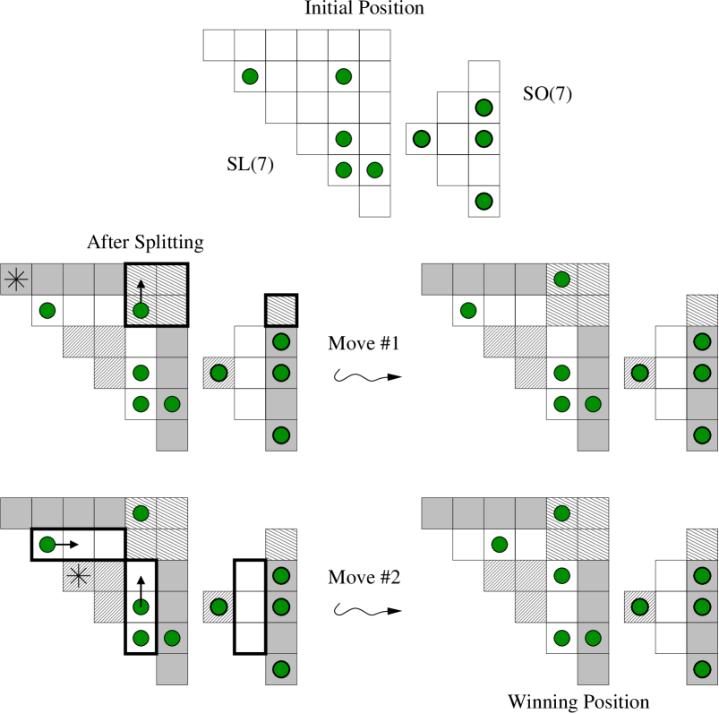
Figure 11: A sequence of moves in the root game for $SO(7)\hookrightarrow SL(7)\times SO(7)$, $\pi=(1425736,\bar{2}3\bar{1})$. The bold outline indicates which region is being used in each move, and the $*$ indicates which root is being used.

Example 4.15.

Let $G=SL(7)\times SO(7)$, $G^{\prime}=SO(7)$, $\pi=(1425736,\bar{2}3\bar{1})$, where $\bar{2}3\bar{1}$ is the $SO(7)$ Weyl group element represented by the matrix

$$\left(\begin{matrix}0&-1&0\\ 0&0&1\\ -1&0&0\end{matrix}\right).$$

Figure 11 shows a sequence of splittings and moves lead to a winning position. Squares belonging to the same region are similarly shaded. For each move, the relevant region is outlined, and the relevant root is indicated by an asterisk in the corresponding square.

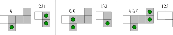
Figure 12: The $3$ games which are doomed for $SL(3)\hookrightarrow G_{2}\times SL(3)$. The shaded squares indicate a minimal ideal subset $A$ for which $\#(\mathcal{T}\cap A)>\#(\hat{\phi}(A)\setminus\{0\})$.

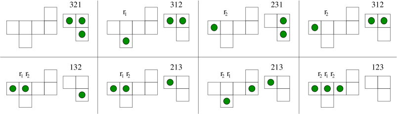
Figure 13: The $8$ games which are not doomed for $SL(3)\hookrightarrow G_{2}\times SL(3)$. Each of these games can be won.

Example 4.16.

Let $G=G_{2}\times SL(3)$, and $G^{\prime}=SL(3)$ including diagonally, where $SL(3)\hookrightarrow G_{2}$ is as described in Example 4.5. We consider all possible $\pi\in W$, with $\ell(\pi)=3=\dim G^{\prime}/B^{\prime}$. There are such $11$ such $\pi$ in total. Of these, $3$ associated games are doomed. These are $\pi=(r_{1},231)$, $\pi=(r_{2}r_{1},132)$, and $\pi=(r_{1}r_{2}r_{1},123)$, where $r_{1}$ and $r_{2}$ represent reflections in the short and long simple roots respectively. These are shown in Figure 12. The remaining $8$ games are shown in Figure 13. One can check that each of these can be won. Figure 14 shows a sequence of moves from the initial position of one of these games, $\pi=(r_{1}r_{2},213)$, to a winning position. Thus the root game gives a complete answer to the vanishing problem for branching $SL(3)\hookrightarrow G_{2}$.

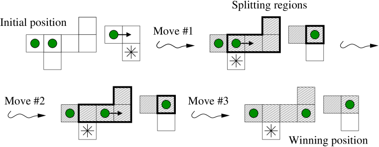
Figure 14: A sequence of moves in the root game for $SL(3)\hookrightarrow G_{2}\times SL(3)$, $\pi=(r_{1}r_{2},213)$. After the first move, we split into three regions, indicated by the different shading of squares. The bold outline indicates which region is being used in each move, and the $*$ indicates which root is being used.

4.4 Specialisation to Schubert intersection numbers

In order to avoid proving Theorems 1 and 2 directly, we show that the formulation of the root game for vanishing of Schubert intersection numbers is in fact just a special case of the more general root game for branching. In the interest of brevity, we’ll call these two formulations of the root game the I-game and the B-game respectively.

As has been already discussed, the correspondence comes from from putting $i:G^{\prime}\hookrightarrow G=G^{\prime}\times\cdots\times G^{\prime}$, the diagonal inclusion.

4.4.1 Token labels versus squares

In the I-game, squares correspond to positive roots of $G^{\prime}$, whereas tokens are labelled $1,\ldots,s$. In the B-game, the squares correspond to positive roots of $G$ and the tokens are unlabelled. The equivalence of the two is seen from the fact that the $\Delta_{+}$ is a disjoint union of $s$ copies of $\Delta^{\prime}_{+}$. The token label in the I-game indicates which copy of $\Delta^{\prime}_{+}$is being used for the corresponding token in the B-game.

4.4.2 Winning condition and splitting

The map $\hat{\phi}:\Delta_{+}\to\Delta^{\prime}_{+}\cup\{0\}$, is given by superimposing all the copies of $\Delta^{\prime}_{+}$. Since $\Delta^{\prime}_{+}$ corresponds to the set of squares in the I-game, the injectivity of $\hat{\phi}|_{\mathcal{T}}$ corresponds to having at most one token in each square. Since we assumed that $\sum\ell(\pi_{i})=\dim G^{\prime}/B^{\prime}$, this is the same as exactly one token in each square.

From this description of $\hat{\phi}$ it is also easy to see that splitting subsets of $\Delta_{+}$ are in one to one correspondence with ideal subsets of $\Delta^{\prime}_{+}$.

4.5 Proofs

4.5.1 Proof of the vanishing criterion

The vanishing criterion (Theorem 4) is a combinatorial reinterpretation of Lemma 2.6.

Proof of Theorem 4.

At the outset, $\{e_{\alpha}\ |\ \alpha\in\mathcal{T}\}$ is a basis for the space $Q$. If the game is doomed then there is an ideal subset $A$ such that $\#(\mathcal{T}\cap A)>\#(\hat{\phi}(A)\setminus\{0\}).$ Let $S\subset\mathfrak{n}$ be the ideal generated by $\{e_{\alpha}\ |\ \alpha\in A\}$. We have

$$\dim(Q\cap S)=\#(\mathcal{T}\cap A)>\#(\hat{\phi}(A)\setminus\{0\})=\dim\phi(S).$$

By Lemma 2.6, we conclude that $i^{*}(\omega_{\pi})=0$. ∎

4.5.2 Proof of the non-vanishing criterion

The non-vanishing criterion (Theorem 5) is essentially combinatorially encoding the geometric ideas in Propositions 2.7 and 2.9.

Proof of Theorem 5.

If $R\subset\Delta_{+}$, we let $\langle e_{\alpha}\ |\ \alpha\in R\rangle_{B}$ denote the $B$-submodule of $\mathfrak{n}$ generated by all $e_{\alpha}$, $\alpha\in R$.

Let $(\mathcal{R}=\{R_{1},\ldots,R_{r}\},\mathcal{T})$ be a position in the root game. We associate to this position the following geometric data:

• $B$-modules $V_{i}$, $i=1,\ldots,r$. Put $V_{i}^{0}=\langle e_{\alpha}\ |\ \alpha\in R_{i}\rangle_{B}$, and $V_{i}^{1}=\langle e_{\alpha}\ |\ \alpha\in\Gamma(V_{i}^{0})\setminus R_{i}\rangle_{B}$. Then we define $V_{i}$ to be the quotient $V_{i}^{0}/V_{i}^{1}$. Note that $V_{i}$ is a $B$-module, and a subquotient of $\mathfrak{n}$, with weights $\Gamma(V_{i})=R_{i}$.

• $B^{\prime}$-modules $V^{\prime}_{i}$, $i=1,\ldots,r$, defined as $V^{\prime}_{i}=\phi(V_{i}^{0})/\phi(V_{i}^{1})$.

• $B^{\prime}$-equivariant maps $\phi_{i}:V_{i}\to V^{\prime}_{i}$, induced from $\phi|_{V_{i}}$.

• Subspaces $U_{i}\subset V_{i}$. $U_{i}$ is defined to be the $T$-invariant subspace of $V_{i}$ with weights $\Gamma(U_{i})=\mathcal{T}\cap R_{i}$.

Thus, for each region $R_{i}$, $i\in\{1,\ldots,r\}$ we have a quadruple $(U_{i},V_{i},V^{\prime}_{i},\phi_{i})$ (as in Section 2.6). Note that the quadruple corresponding to the initial position is $(Q,\mathfrak{n},\mathfrak{n}^{\prime},\phi)$.

We claim that if a root game can be won, then every such quadruple encountered over the course of the game is good. In particular the initial position is good, which, by Lemma 2.4 implies that $i^{*}(\omega_{\pi})\neq 0$.

First, we note that the quadruples $(U_{i},V_{i},V^{\prime}_{i},\phi_{i})$ associated to a winning position are good. Indeed, if $\mathcal{T}$ is injective, then $\phi_{i}|_{U_{i}}:U_{i}\to V^{\prime}_{i}$ is an injective linear map, thus $(U_{i},V_{i},V^{\prime}_{i},\phi_{i})$ is good.

To establish the claim we must show two things:

1. Suppose $(\mathcal{R},\mathcal{T})$ is the position of a root game before a move $[\beta,R_{j}]$, and $(\mathcal{R},\mathcal{T}^{\prime})$ is the position after the move. If all quadruples associated to $(\mathcal{R},\mathcal{T}^{\prime})$ are good, then all quadruples associated to $(\mathcal{R},\mathcal{T})$ are good.

2. Suppose $(\mathcal{R},\mathcal{T})$ is the position of a root game before splitting along a splitting subset $A$, and $(\mathcal{R}^{\prime},\mathcal{T})$ is the position after the splitting. If all quadruples associated to $(\mathcal{R}^{\prime},\mathcal{T})$ are good, then all quadruples associated to $(\mathcal{R},\mathcal{T})$ are good.

Proof of (i): All quadruples $(U_{i},V_{i},V^{\prime}_{i},\phi_{i})$, $i\neq j$, are unchanged by the move $[\beta,R_{j}]$. The position $(U_{j},V_{j},V^{\prime}_{j},\phi_{j})$, however, is changed to $(U_{j}^{1},V_{j},V^{\prime}_{j},\phi_{j})$, where $\Gamma(U_{j}^{1})=\Gamma(U_{j})\boxplus_{R_{j}}\beta$. By Lemma 2.8, $U_{j}^{1}=\lim_{t\to\infty}\theta_{\beta}(t)\cdot U_{j}$, and thus (i) follows by Proposition 2.7.

Proof of (ii): Let $S=\langle e_{\alpha}\ |\ \alpha\in A\rangle$ be the ideal of $\mathfrak{n}$ corresponding to $A$. Let $S_{i}$ be the corresponding submodule of $V_{i}$: $S_{i}=S\cap V_{i}^{0}/V_{i}^{1}$. Put $S^{\prime}_{i}=\phi_{i}(S_{i})$. We let $q_{i}:V_{i}\to V_{i}/S_{i}$, and $q^{\prime}_{i}:V^{\prime}_{i}\to V^{\prime}_{i}/S_{i}$, denote the quotient maps.

The result of splitting the region $R_{i}\in\mathcal{R}$ along $A$ is two regions: $R_{i}\cap A$ and $R_{i}\cap A^{c}$. Let $(U_{i},V_{i},V^{\prime}_{i},\phi_{i})$ be the quadruple associate to $R_{i}$. Then the quadruple associated to $R_{i}\cap A$ is $(U_{i}\cap S_{i},S_{i},S^{\prime}_{i},\phi_{i}|S_{i})$, and the quadruple associated $R_{i}\cap A^{c}$ $(q(U_{i}),V_{i}/S_{i},V^{\prime}_{i}/S^{\prime}_{i},q^{\prime}_{i}\circ\phi_{i}\circ q_{i}^{-1})$. (The latter, is because $A$ is a splitting subset (not merely an ideal subset), thus $\phi$ respects not just the weight spaces of $S_{i},S^{\prime}_{i}$, but also the complementary weight spaces.) Using Proposition 2.9, (ii) follows.

∎

References

- [B] P. Belkale, Geometric Proofs of Horn and Saturation Conjectures, J. Alg. Geom. 15 (2006), no. 1, 133–173.
- [BS] A. Berenstein, R. Sjamaar, Coadjoint orbits, moment polytopes, and the Hilbert-Mumford criterion. J. Amer. Math. Soc. 13 (2000), no. 2, 433–466 (electronic).
- [BH] S. Billey, M. Haiman, Schubert polynomials for the classical groups. J. Amer. Math. Soc. 8 (1995), no. 2, 443–482.
- [F] W. Fulton, Young Tableaux with Applications to Representation Theory and Geometry, Cambridge U.P., New York, 1997.
- [GS] V. Guillemin, S. Sternberg, Convexity properties of the moment mapping, Invent. Math. 67 (1982), no. 3, 491–513.
- [GLS] V. Guillemin, E. Lerman, S. Sternberg, Symplectic fibrations and multiplicity diagrams, Cambridge University Press, Cambridge, 1996.
- [H] G. J. Heckman, Projections of orbits and asymptotic behavior of multiplicities for compact connected Lie groups, Invent. Math. 67 (1982), no. 2, 333–356.
- [Kl] S. Kleiman, The transversality of a general translate, Compositio Math. 28 (1974), 287-297.
- [Kn] A. Knutson, Descent-cycling in Schubert calculus, Experiment. Math. 10 (2001), no. 3, 345–353
- [LS] A. Lascoux, M.-P. Schützenberger, Polynômes de Schubert, R. Acad. Sci. Paris Sér. I Math. 294 (1982), no. 13, 447–450 (French)
- [P1] K. Purbhoo, Root games on Grassmannians, preprint math.CO/0310103.
- [P2] K. Purbhoo, Vanishing and non-vanishing criteria for branching Schubert calculus, Ph.D. Thesis, U.C. Berkeley, 2004.
- [P3] K. Purbhoo, Two step flag manifolds and the Horn conjecture, in preparation.