Sextic surfaces with ten triple points

Abstract

All families of sextic surfaces with the maximal number of isolated triple points are found.

Surfaces in ${\mathbb{P}}^{3}({\mathbb{C}})$ with isolated ordinary triple points have been studied in [EPS]. The results are most complete for degree six. A sextic surface can have at most ten triple points, and such surfaces exist. For up to nine triple points [EPS] contains a complete classification. In this note I achieve the same for ten triple points.

The study of sextics with nine triple points is easier, because they do lie on a quadric $Q$, which is not the case for ten points. Given such a sextic with equation $F$ the general element of the pencil $\alpha F+\beta Q^{3}$ is again a sextic with nine isolated triple points. It turns out that such a pencil also contains reducible surfaces, which are much easier to construct. The same argument shows that a sextic with ten triple points is a degeneration of one with nine (simply choose a quadric through nine of the ten points).

Therefore one can look for sextics with ten triple points in each of the five families given in [EPS]. It suffices to consider only those two,which have a rather nice description. The one-parameter family of examples [EPS] was found in the first family by imposing extra symmetry. The surfaces in the other family have the simplest equations of all. Nevertheless I could not find a single solution, because I was looking at the wrong place: as explained below, I made an unwarranted general position assumption. Different families of sextics are connected by Cremona transformations. By transforming the known example I found the right assumptions. The equations for a tenth triple point in the family become very simple, as I had hoped all the time. They describe a three-dimensional family. Knowing the dimension then helped to find all solutions in the other family.

To solve the equations I use the computer algebra system Singular [GPS]. The equations for the tenth point come from the ten second partial derivatives of the defining function. The families with nine triple points depend on seven or eight moduli. The unknown position of the tenth singular point adds three more variables. One gets a very complicated system, which only can be attacked by using the special structure of the equations.

The main result is that there are four different families of sextics with ten triple points, each depending on three moduli. They are distinguished by the number of $(-1)$-conics, which ranges from two to five.

1 Nine triple points

The clue to the classification of sextics with many triple points is the study of exceptional curves of the first kind on the minimal resolution. Let $X$ be a sextic with isolated triple points and $\widetilde{X}$ its minimal resolution. Whenever the canonical divisor $K_{\widetilde{X}}$ is effective, any exceptional curve of the first kind $E$ is automatically a component, as $K_{\widetilde{X}}\cdot E=-1$. Therefore $E$ comes from a rational curve on $X$ which is contained in the base locus of the system of quadrics through the triple points. Assume that $X$ has nine triple points $P_{1},\ldots,P_{9}$. Let $Q$ be the unique (irreducible) canonical quadric surface and let $K=Q\cdot X$ be the adjoint curve. The resolution $\widetilde{X}$ has exactly three disjoint $(-1)$-curves $C_{1},C_{2},C_{3}$ of degrees $c_{1},c_{2},c_{3}\in\{2,4,5,6,7,8\}$ which are components of $K$. There are two possibilities: either $C_{1}+C_{2}+C_{3}=K$ or not. In the first case $\widetilde{X}$ is a $K3$ surface blown up in three points. By [EPS], Prop. 4.10, there are up to permutation three choices for the degrees:

$$(c_{1},c_{2},c_{3})\in\{(2,2,8),(2,4,6),(4,4,4)\}.$$

In the second case we end up with an effective canonical divisor after blowing down $C_{1}$, $C_{2}$ and $C_{3}$. Now $\widetilde{X}$ is the blowup of a minimal properly elliptic surface in three points and by [EPS], Prop. 4.9, up to permutation

$$(c_{1},c_{2},c_{3})\in\{(2,2,2),(2,2,4)\}.$$

In all cases the curves $C_{i}$ of degree $c_{i}$ can be constructed as complete intersection of $Q$ and a surface of degree $c_{i}/2$. In particular, if $c_{i}=2$ we have five points on a conic in a plane. Such a conic will be called a $(-1)$-conic. We call the triple $(c_{1},c_{2},c_{3})$ the type of the surface.

For every $(c_{1},c_{2},c_{3})\in\{(2,2,8),(2,4,6),(4,4,4)\}$ there exists a seven parameter family of sextic surfaces with nine triple points and three $(-1)$-curves of degrees $c_{1}$, $c_{2}$ and $c_{3}$ ([EPS], Thm. 4.13). Moreover $X$ occurs in a pencil of the form

$$\begin{array}[]{r@{\quad}l}\alpha\,K_{1}K_{2}K_{3}+\beta\,Q^{3}=0\;,&\mathrm{if}\ (c_{1},c_{2},c_{3})=(4,4,4)\;,\\[4.30554pt] \alpha\,L_{1}K_{2}C_{3}+\beta\,Q^{3}=0\;,&\mathrm{if}\ (c_{1},c_{2},c_{3})=(2,4,6)\;,\\[4.30554pt] \alpha\,L_{1}L_{2}Q_{3}+\beta\,Q^{3}=0\;,&\mathrm{if}\ (c_{1},c_{2},c_{3})=(2,2,8)\;.\end{array}$$

Here $Q$ is the unique canonical surface, $L_{i}$ stands for a linear form, $K_{i}$ for a singular quadric, $C_{3}$ defines a four nodal cubic and $Q_{3}$ a quartic surface with a triple point and six double points. The multiplicities of the three surfaces in the nine singular points are displayed in Table 1. Note that we do not distinguish between a surface and the form defining it, which we also call its equation.

type	surface	$P_{1}$	$P_{2}$	$P_{3}$	$P_{4}$	$P_{5}$	$P_{6}$	$P_{7}$	$P_{8}$	$P_{9}$
	$K_{1}$	0	2	1	1	1	1	1	1	1
$(4,4,4)$	$K_{2}$	1	0	2	1	1	1	1	1	1
	$K_{3}$	2	1	0	1	1	1	1	1	1
	$L_{1}$	1	0	0	0	0	1	1	1	1
$(2,4,6)$	$K_{2}$	0	2	1	1	1	1	1	1	1
	$C_{3}$	2	1	2	2	2	1	1	1	1
	$L_{1}$	1	0	0	0	0	1	1	1	1
$(2,2,8)$	$L_{2}$	0	1	1	1	0	0	0	1	1
	$Q_{3}$	2	2	2	2	3	2	2	1	1

Table 1: multiplicities at the singular points in the $K3$-case

Figure 1 shows a surface of type $(4,4,4)$. The picture was made with Stephan Endraß’ program surf [En].

For every $(c_{1},c_{2},c_{3})\in\{(2,2,2),(2,2,4)\}$ there exists an eight parameter family of sextic surfaces with nine triple points and three $(-1)$-curves of degrees $c_{1}$, $c_{2}$ and $c_{3}$ ([EPS], Thm. 4.14). Moreover $X$ occurs in a web of the form

$$\begin{array}[]{r@{}c@{}c@{\quad}l}\alpha\,L_{1}L_{2}L_{3}C+{}&\beta\,L_{1}L_{2}L_{3}HQ&{}+\gamma\,Q^{3}=0\;,&\mathrm{if}\ (c_{1},c_{2},c_{3})=(2,2,2)\;,\\[4.30554pt] \alpha\,L_{1}L_{2}K_{3}Q^{\prime}+{}&\beta\,L_{1}L_{2}K_{3}Q&{}+\gamma\,Q^{3}=0\;,&\mathrm{if}\ (c_{1},c_{2},c_{3})=(2,2,4)\;.\end{array}$$

Again $L_{i}$ stands for a linear form. In the case $(2,2,2)$ the plane $H$ passes through the three triple points not lying on the double lines of $L_{1}L_{2}L_{3}$. The reducible cubic $HQ$ is an element of the pencil of cubics through all points with double points in $P_{7}$, $P_{8}$ and $P_{9}$, and $C$ is another such cubic. In the case $(2,2,4)$ the surface $K_{3}$ is a quadric cone and $Q^{\prime}$ is a smooth quadric not passing through $P_{6}$. The multiplicities in the nine triple points of the surfaces giving $(-1)$-curves are displayed in Table 2. A surface of type $(2,2,2)$ is shown in Figure 2.

Figure 1: A surface of type $(4,4,4)$ with nine triple points

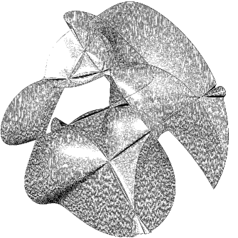
Figure 2: A surface of type $(2,2,2)$ with nine triple points

type	surface	$P_{1}$	$P_{2}$	$P_{3}$	$P_{4}$	$P_{5}$	$P_{6}$	$P_{7}$	$P_{8}$	$P_{9}$
	$L_{1}$	0	0	1	1	1	1	1	0	0
$(2,2,2)$	$L_{2}$	1	1	0	0	1	1	0	1	0
	$L_{3}$	1	1	1	1	0	0	0	0	1
	$L_{1}$	0	0	1	1	1	1	1	0	0
$(2,2,4)$	$L_{2}$	1	1	0	0	1	1	0	1	0
	$K_{3}$	1	1	1	1	0	1	1	1	2

Table 2: multiplicities in the properly elliptic case

The three families of blown-up $K3$-surfaces are related via Cremona transformations. The ordinary plane Cremona transformation is the rational map defined by the linear system of conics through three points in general position. In suitable coordinates it can be given by the formula $(x\mathop{\rm:}y\mathop{\rm:}z)\mapsto(1/x\mathop{\rm:}1/y\mathop{\rm:}1/z)$. This formula generalises to higher dimensions. In particular, the space transformation, also known as reciprocal transformation,

$$(x\mathop{\rm:}y\mathop{\rm:}z\mathop{\rm:}w)\mapsto\left(\frac{1}{x}\mathop{\rm:}\frac{1}{y}\mathop{\rm:}\frac{1}{z}\mathop{\rm:}\frac{1}{w}\right)$$

simultaneously blows up the vertices and blows down the faces of the coordinate tetrahedron. The vertices are called fundamental points of the reciprocal transformation. Let $X\subset{\mathbb{P}}^{3}$ by a surface of degree $d$ not containing any of the coordinate planes. Let $m_{1}$, …, $m_{4}$ be the multiplicities of $X$ in the fundamental points. Then the image $Y$ of $X$ is a surface of degree $3d-m_{1}-\cdots-m_{4}$. In many cases $X$ will be singular in the fundamental points with singularities obtained from contracting the intersection curves of $X$ with the coordinate planes.

Specifically, a reciprocal transformation with fundamental points $P_{1}$, $P_{2}$, $P_{4}$ and $P_{5}$ will transform a surface of type $(4,4,4)$ into one of type $(2,4,6)$. To get from there to a surface of type $(2,2,8)$ we can apply a transformation with fundamental points $P_{2}$, $P_{5}$, $P_{6}$ and $P_{7}$, where the points are as in Table 1. The two other families are also related via reciprocal transformations.

2 Families with ten triple points

For a sextic surface $X$ with ten isolated triple points $p_{g}(\widetilde{X})=0$ ([EPS], Cor. 4.6) so the ten points never lie on a quadric. Leaving out one point the remaining nine triple points determine a quadric $Q$. The general element of the pencil spanned by our sextic and $Q^{3}$ is a surface with nine isolated triple points and belongs therefore at least to one of the five families above.

Lemma 1

A sextic with ten triple points belongs to the closure of the family of type $(2,2,2)$ or of the family of type $(4,4,4)$.

Proof.  No three triple points lie on a line ([EPS], Lemma 3.1). Two different $(-1)$-conics meet in two triple points ([EPS], Cor. 4.8). We study the planes containing $(-1)$-conics. If three planes have a line in common, there would be $2+3\cdot 3=11$ triple points; if four plane have a triple point in common, they contain $1+6+4=11$ points, again contradicting that the surface has ten triple points. The number of planes is at most six. If there are exactly six, then each triple point lies in three planes, and leaving out one of the points gives sextics with three planes, so of type $(2,2,2)$. If there are five planes, we have ten lines each containing two triple points, so five points lie in three planes and five only in two. Leaving out a point in only two planes gives a sextic of type $(2,2,2)$. If there are four planes and only one point lies in three of them, the fourth plane contains six points. So there are at least two points in three planes each. A plane containing them both has only four points on intersection lines so leaving out the fifth point in such a plane gives a sextic of type $(2,2,2)$. If there are three planes, they can contain at most nine points, so by leaving out the point not on a plane we keep three planes. If there are only two planes we can leave out a point on the intersection line to get sextics without planes, so of type $(4,4,4)$. If there is only one plane we leave out any point in that plane.     $\Box$

2.1 Type $(2,2,2)$

We describe equations for the surfaces. After a change of coordinates we may assume that the three planes are the sides of the coordinate tetrahedron. The remaining coordinate transformations are given by diagonal matrices. We have two points on each axis in affine space and three additional ones on the triangle at infinity. We take them to be $P_{7}=(0\mathop{\rm:}1\mathop{\rm:}\lambda\mathop{\rm:}0)$, $P_{8}=(\mu\mathop{\rm:}0\mathop{\rm:}1\mathop{\rm:}0)$ and $P_{9}=(1\mathop{\rm:}\nu\mathop{\rm:}0\mathop{\rm:}0)$. The equation has now the form

$$\alpha\;Q^{3}+\beta\;xyztQ+\gamma\;xyzK\;,$$

with $K$ is a four-nodal cubic passing through $(0\mathop{\rm:}0\mathop{\rm:}0\mathop{\rm:}1)$. With notation slightly different from [EPS] we get

$$Q = c_{1}c_{2}c_{3}t^{2}+t(b_{1}c_{2}c_{3}x+b_{2}c_{1}c_{3}y+b_{3}c_{1}c_{2}z)$$

$${}+c_{2}c_{3}x(\nu x-y-\mu\nu z)+c_{1}c_{3}y(\lambda y-z-\lambda\nu x)+c_{1}c_{2}z(\mu z-x-\lambda\mu y)\;,$$

$$K = t^{2}(\lambda\nu c_{1}x+\lambda\mu c_{2}y+\mu\nu c_{3}z)$$

$${}+t\big{(}\lambda b_{1}x(\nu x-y-\mu\nu z)+\mu b_{2}y(\lambda y-z-\lambda\nu x)+\nu b_{3}z(\mu z-x-\lambda\mu y)\big{)}$$

$${}+(\nu x-y-\mu\nu z)(\lambda y-z-\lambda\nu x)(\mu z-x-\lambda\mu y)\;.$$

We use the remaining freedom in coordinate transformations to place the putative tenth triple point in $(1\mathop{\rm:}1\mathop{\rm:}1\mathop{\rm:}1)$. We compute in the affine chart $t=1$. The condition for a triple point is then that the function, its derivatives and the second order derivatives vanish at $(1,1,1)$. This gives ten equations which are linear in $\alpha$, $\beta$ and $\gamma$, so we may eliminate them: the maximal minors of the coefficient matrix have to vanish. We have

$$\frac{\partial Q^{3}}{\partial x} = 3Q^{2}Q_{x}\;,$$

$$\frac{\partial^{2}Q^{3}}{\partial x^{2}} = 3Q^{2}Q_{xx}+6QQ_{x}^{2}\;,$$

$$\frac{\partial^{2}Q^{3}}{\partial x\partial y} = 3Q^{2}Q_{xy}+6QQ_{x}Q_{y}\;.$$

All these expressions are divisible by $Q$.

Now we plug in $x=y=z=1$. From $Q$ we get

$$\halign{\hbox to\displaywidth{$\hfil\displaystyle#\hfil$}\cr 0.0pt{\hfil$\displaystyle\quad Q(1,1,1)\hfill\cr 0.0pt{\hfil$\displaystyle\hfill\qquad{}=c_{1}c_{2}c_{3}+c_{2}c_{3}(b_{1}+\nu-1-\mu\nu)+c_{1}c_{3}(b_{2}+\lambda-1-\lambda\nu)+c_{1}c_{2}(b_{3}+\mu-1-\lambda\mu)\;,\;\crcr}}}$$

an expression which we continue to denote by $Q$. We also get expressions for all derivatives. Likewise we have

$$K = \lambda\nu c_{1}+\lambda\mu c_{2}+\mu\nu c_{3}$$

$${}+\lambda b_{1}(\nu-1-\mu\nu)+\mu b_{2}(\lambda-1-\lambda\nu)+\nu b_{3}(\mu-1-\lambda\mu)$$

$${}+(\nu-1-\mu\nu)(\lambda-1-\lambda\nu)(\mu-1-\lambda\mu)\;.$$

Furthermore

$$\left.\frac{\partial\,xyzK}{\partial x}\;\right|_{(1,1,1)} = (yzK+xyzK_{x})_{|_{(1,1,1)}}=K+K_{x}\;,$$

$$\left.\frac{\partial^{2}\,xyzK}{\partial x^{2}}\;\right|_{(1,1,1)} = (2yzK_{x}+xyzK_{xx})_{|_{(1,1,1)}}=2K_{x}+K_{xx}\;,$$

$$\left.\frac{\partial^{2}\,xyzK}{\partial x\partial y}\;\right|_{(1,1,1)} = (zK+xzK_{x}+yzK_{y}+xyzK_{xy})_{|_{(1,1,1)}}$$

$$\qquad\qquad{}=K+K_{x}+K_{y}+K_{xy}\;.$$

After dividing the first row by $Q$, which is allowed because the tenth triple point does not lie on the quadric $Q$, our matrix has the following form:

$$\pmatrix{Q^{2}&3QQ_{x}&\ldots&3QQ_{xx}+6Q_{x}^{2}&\ldots&3QQ_{xy}+6Q_{x}Q_{y}&\ldots\cr Q&Q+Q_{x}&\ldots&2Q_{x}+Q_{xx}&\ldots&Q+Q_{x}+Q_{y}+Q_{xy}&\ldots\cr K&K+K_{x}&\ldots&2K_{x}+K_{xx}&\ldots&K+K_{x}+K_{y}+K_{xy}&\ldots}\;.$$

The vanishing of the maximal minors is the necessary condition for multiplicity $3$ in the point $(1,1,1)$, but it is not sufficient for the existence of a surface with only isolated singularities. We have to cut away unwanted solutions, like $Q=Q_{x}=Q_{y}=Q_{z}=0$, which makes all minors vanish, but does not give isolated triple points. The minors are rather formidable expressions. We first try to simplify the matrix itself.

We start by subtracting $3Q$ times the second row from the first row to remove all second derivatives from the first row. After that we apply only column operations. Some experimentation with the matrix showed that it is possible to get two zeroes in one column. We observe that $Q_{xx}+2\nu Q_{xy}+\nu^{2}Q_{yy}=0$. Note that one can write $Q(x,y,z,t)=\frac{1}{2}Q_{xx}x^{2}+Q_{xy}xy+\cdots+\frac{1}{2}Q_{tt}t^{2}$, as the second derivatives are constants. The identity $Q_{xx}+2\nu Q_{xy}+\nu^{2}Q_{yy}=0$ now follows from the fact that the point $(1\mathop{\rm:}\nu\mathop{\rm:}0\mathop{\rm:}0)$ lies on the quadric. The same point is a double point of the cubic $K$, so all first derivatives vanish, giving by the same argument that $(K_{w})_{xx}+2\nu(K_{w})_{xy}+\nu^{2}(K_{w})_{yy}=0$, where $w$ is one of $(x,y,z,t)$. Applying Euler’s relation $3K=xK_{x}+yK_{y}+zK_{z}+tK_{t}$ in the point $(1\mathop{\rm:}1\mathop{\rm:}1\mathop{\rm:}1)$ yields by adding that also $K_{xx}+2\nu K_{xy}+\nu^{2}K_{yy}=0$, where now $K_{xx}$ again stands for the second derivative evaluated in $(1,1,1)$. Equivalent equations hold for the other second partials.

We get in this way three columns with two zeroes by elementary column operations, if we multiply one column, say the one containing containing $Q_{xx}$, with $1+\lambda\mu\nu$. The vanishing of this factor expresses that the three points $P_{7}$, $P_{8}$ and $P_{9}$ lie on a line, so we may introduce new unwanted solutions, which we cut away later in the computation. The result is

$$\pmatrix{-2Q^{2}&-Q^{2}&\ldots&Q^{2}-3QQ_{x}-3QQ_{y}+6Q_{x}Q_{y}&\ldots&E_{\nu}&\ldots\cr Q&Q_{x}&\ldots&Q_{xy}&\ldots&0&\ldots\cr K&K_{x}&\ldots&K_{xy}&\ldots&0&\ldots},$$

where $E_{\nu}$ is the first of three similar equations

$$\begin{array}[]{lc}E_{\nu}\colon&(\nu^{2}+\nu+1)Q^{2}-3(\nu+1)Q(\nu Q_{y}+Q_{x})+3(\nu Q_{y}+Q_{x})^{2}\;,\\ E_{\lambda}\colon&(\mu^{2}+\mu+1)Q^{2}-3(\mu+1)Q(\mu Q_{x}+Q_{z})+3(\mu Q_{x}+Q_{z})^{2}\;,\\ E_{\mu}\colon&(\lambda^{2}+\lambda+1)Q^{2}-3(\lambda+1)Q(\lambda Q_{z}+Q_{y})+3(\lambda Q_{z}+Q_{y})^{2}\;.\end{array}$$

These equations have to hold, for if $E_{\nu}\neq 0$, then $\alpha=0$ and the equation for the sextic is divisible by $xyz$. Considered as quadratic equation in $Q$ and $\nu Q_{y}+Q_{x}$ the equation $E_{\nu}$ has discriminant $-3(\nu-1)^{2}$. The case $\nu=1$ is excluded: if $\nu=1$ then $0=Q_{x}+Q_{y}-Q=c_{1}c_{2}(c_{3}+b_{3}+\mu)$, which means that the point $(0,0,1)$ is a triple point, which lies on the line through the tenth point $(1,1,1)$ and $P_{9}=(1\mathop{\rm:}1\mathop{\rm:}0\mathop{\rm:}0)$. Therefore no solution is defined over ${\mathbb{R}}$. We have to adjoin $\sqrt{-3}$ or what amounts to the same, the third roots of unity.

By factorising $E_{\kappa}$, $\kappa=\lambda,\mu,\nu$, we get linear equations, which express $Q_{x}+\nu Q_{y}$, $Q_{y}+\lambda Q_{z}$ and $Q_{z}+\mu Q_{x}$ as multiples of $Q$. To express $Q_{x}$, $Q_{y}$ and $Q_{z}$ themselves as multiples of $Q$ we have to multiply with the determinant $1+\lambda\mu\nu$ of the system. By doing so to the fifth, sixth and seventh column of our matrix we can get use the first column to get zeroes on the first row in all other columns. This reduces our problem to the minors of a $(2\times 6)$-matrix.

The analysis up to this point is basically contained in [EPS]. To proceed further we note that our three linear equations are in fact linear in $b_{1}c_{2}c_{3}$, $b_{2}c_{1}c_{3}$ and $b_{3}c_{1}c_{2}$. Therefore they can be used to eliminate the $b_{i}$. For the second row this is quite easy to do: by column operations we can remove the $b_{i}$ from column 5, 6 and 7 and then we take suitable linear combinations of columns 2, 3 and 4 with coefficients polynomials in $(\lambda,\mu,\nu)$ such that the entries on the second row have the same coefficients at the $b_{i}c_{i}jc_{k}$ as our three equations. For the third row one has to first multiply with a quite complicated determinant, which leads to long expressions. At this stage the use of the computer becomes indispensable. The new second column turns out to be divisible by $\nu-1$, and likewise the third by $\lambda-1$, the fourth by $\mu-1$. After division the entries $(2,2)$, $(2,3)$ and $(2,4)$ are equal, which means that we again get columns with two zeroes, giving two equations. From the remaining $(2\times 4)$-matrix we take the 6 maximal minors. Now we have a system of 8 rather complicated equations in 6 variables. We still have to cut away unwanted solutions, those lying in $Q=0$, $\lambda\mu\nu+1=0$, $\lambda=1$, $\mu=1$, $\nu=1$ and $c_{i}=0$. This can be done in Singular as follows. First we homogenise with an extra variable $h$. To cut away the solutions in $Q=0$ we adjoin the inhomogeneous equation $Q-1$, where $Q$ is made homogeneous with $h$, and compute a standard basis. Then we homogenise again with $Q$. By doing the same for the other unwanted solutions we finally obtain equations of reasonably low degree. To do the calculation in reasonable time it is best to compute over a finite field ${\mathbb{Z}}/p{\mathbb{Z}}$ containing the third roots of unity. One can then try to lift the result to characteristic zero and check whether the guessed equations really solve the system.

Let $\varepsilon$ be a primitive third root of unity. We first take the same root to solve the three equations $E_{\kappa}$:

$$3(\nu Q_{y}+Q_{x})-((1-\varepsilon^{2})\nu+(1-\varepsilon))Q = 0\;,$$

$$3(\mu Q_{x}+Q_{z})-((1-\varepsilon^{2})\lambda+(1-\varepsilon))Q = 0\;,$$

$$3(\lambda Q_{z}+Q_{y})-((1-\varepsilon^{2})\mu+(1-\varepsilon))Q = 0\;.$$

By eliminating $c_{2}$ and $c_{3}$ we end up with one equation which is quadratic in $c_{1}$, so we find a three dimensional solution space. The equations are rather involved.

A cyclic permutation of the variables $(x,y,z)$ in the original configuration induces a cyclic permutation of each of the triples $(b_{1},b_{2},b_{3})$, $(c_{1},c_{2},c_{3})$ and $(\lambda,\mu,\nu)$. A transposition of $x$ and $y$ has a more complicated effect on the coefficients. On the points $P_{7}$, $P_{8}$, $P_{9}$ it acts as $(0\mathop{\rm:}1\mathop{\rm:}\lambda\mathop{\rm:}0)\mapsto(1\mathop{\rm:}0\mathop{\rm:}\lambda\mathop{\rm:}0)=(1/\lambda\mathop{\rm:}0\mathop{\rm:}1\mathop{\rm:}0)$, $(\mu\mathop{\rm:}0\mathop{\rm:}1\mathop{\rm:}0)\mapsto(0\mathop{\rm:}\mu\mathop{\rm:}1\mathop{\rm:}0)=(0\mathop{\rm:}1\mathop{\rm:}1/\mu\mathop{\rm:}0)$ and $(1\mathop{\rm:}\nu\mathop{\rm:}0\mathop{\rm:}0)\mapsto(\nu\mathop{\rm:}1\mathop{\rm:}0\mathop{\rm:}0)=(1\mathop{\rm:}1/\nu\mathop{\rm:}0\mathop{\rm:}0)$. The induced action on the coefficients is therefore $((\lambda,\mu,\nu)\mapsto(1/\mu\mathop{\rm:}1/\lambda\mathop{\rm:}1/\nu)$. By also considering $P_{1}$, …, $P_{6}$ we find that $(c_{1},c_{2},c_{3})\mapsto(c_{2}/\lambda\nu,c_{1}/\mu\nu,c_{3}/\lambda\mu)$ and $(b_{1},b_{2},b_{3})\mapsto(b_{2}/\lambda\nu,b_{1}/\mu\nu,b_{3}/\lambda\mu)$. We clear denominators in $Q(x,y,z)$ and $K(x,y,z)$. The equation $3(\nu Q_{y}+Q_{x})-((1-\varepsilon^{2})\nu+(1-\varepsilon))Q=0$ is transformed into $3(\nu Q_{y}+Q_{x})-((1-\varepsilon^{2})+(1-\varepsilon)\nu)Q=0$ (where we multiplied with $\nu$ to avoid denominators). By taking a particular normal form of the family we found two components, one with $\varepsilon$ and one with $\varepsilon^{2}$, but the surfaces in those components are isomorphic. As the permutation of $x$ and $y$ is isotopic to the identity there is only one component (of dimension $3+15$) in the space of all sextics.

Now we take different roots of unity in the equations $E_{\kappa}$. By using the permutations of $(x,y,z)$ it suffices to consider:

$$3(\nu Q_{y}+Q_{x})-((1-\varepsilon^{2})\nu+(1-\varepsilon))Q = 0\;,$$

$$3(\mu Q_{x}+Q_{z})-((1-\varepsilon^{2})\lambda+(1-\varepsilon))Q = 0\;,$$

$$3(\lambda Q_{z}+Q_{y})-((1-\varepsilon)\mu+(1-\varepsilon^{2}))Q = 0\;.$$

We start the computation as described above. The two equations coming from the second row of the matrix factorise. Disregarding a factor $(\lambda\mu\nu+1)$ we find the equations

$$\halign{\hbox to\displaywidth{$\hfil\displaystyle#\hfil$}\cr 0.0pt{\hfil$\displaystyle(\lambda\mu c_{2}-c_{3})\left(\nu c_{1}c_{2}c_{3}-(\nu(\varepsilon^{2}+\lambda)c_{1}c_{3}-\nu c_{2}c_{3}-\varepsilon c_{1}c_{2})(\mu\nu-\nu+1)\right)\;,\cr 0.0pt{\hfil$\displaystyle(\lambda\nu c_{1}-c_{2})\left(\mu c_{1}c_{2}c_{3}-((\varepsilon\nu+1)c_{1}c_{3}-\varepsilon^{2}\mu\nu c_{2}c_{3}-\mu c_{1}c_{2})(\lambda\mu-\mu+1)\right)\;.\crcr}}}$$

Applying a suitable transposition of the coordinates induces a transformation which sends the first equation to the second one with $\varepsilon$ replaced by $\varepsilon^{2}$.

We find one three dimensional solution by taking both long factors. Then we find $\mu c_{2}=(\lambda\mu-\mu+1)(\mu\nu-\nu+1)$ and a quadratic equation in $c_{1}$, which I do not describe here.

Another three dimensional solution is found by taking the equations $\lambda\mu c_{2}-c_{3}$ and $\mu c_{1}c_{2}c_{3}-((\varepsilon\nu+1)c_{1}c_{3}-\varepsilon^{2}\mu\nu c_{2}c_{3}-\mu c_{1}c_{2})(\lambda\mu-\mu+1)$. The other possible choice gives a solution, isomorphic to the complex conjugate of this one. It might seem that we get two different solutions, but as we shall show, the surfaces in question can also be written in a different way as a degeneration of a sextic of type $(2,2,2)$. By computing for a specific example we find that both solutions are slices of the same component in the space of all sextics. This time we find a linear equation for $c_{1}$:

$$c_{1}+\varepsilon^{2}(\lambda\mu-\mu+1)(\lambda\mu\nu+\varepsilon\mu\nu-\varepsilon\nu-\varepsilon^{2})=0\;.$$

We have already $c_{3}=\lambda\mu c_{2}$ and we find

$$(\lambda\mu\nu+\varepsilon\mu\nu+\varepsilon^{2}\nu-\varepsilon^{2})c_{3}+\varepsilon(\varepsilon\lambda\nu+\lambda-1)c_{1}=0\;.$$

Finally, taking $c_{3}=\lambda\mu c_{2}$ and $c_{2}=\lambda\nu c_{1}$ gives a two dimensional solution consisting of two components, one of which lies inside the last component just found, and the other in the one obtained by interchanging the equations.

Proposition 2

The family of sextic surfaces of type $(2,2,2)$ with nine triple points contains in its closure three different families of sextics with ten triple points, which contain three, four or five $(-1)$-conics.

Proof.  We have already seen that there are at most three different families. We distinguish between them with the number of $(-1)$-conics. A $(-1)$-conic determines a plane, whose intersection with one of the three coordinate planes can have at most two triple points. It has to contain at least two of the points $P_{1}$, …, $P_{6}$ on the coordinate axes, because $P_{7}$, $P_{8}$, $P_{9}$ and $P_{10}$ are not coplanar. But if the plane contains a point on a coordinate axis, it contains only two other triple points on the coordinate planes through the point and therefore it contains the two points not in these planes. If there are three points of the points $P_{1}$, …, $P_{6}$ in the plane, it therefore contains again $P_{7}$, $P_{8}$, $P_{9}$ and $P_{10}$. Therefore there are only three possible planes which can contain a $(-1)$-conic, namely the planes through $P_{10}$ and two of $P_{7}$, $P_{8}$ and $P_{9}$. The equation for the plane through $P_{7}$, $P_{8}$ and $P_{10}$ is $\mu z-x-\lambda\mu y+\lambda\mu-\mu+1$.

To determine the number of $(-1)$-conics in each family it suffices to do it for a specific example. We obtain three conditions by requiring that the points $(1\mathop{\rm:}0\mathop{\rm:}0\mathop{\rm:}1)$, $(0\mathop{\rm:}1\mathop{\rm:}0\mathop{\rm:}1)$ and $(0\mathop{\rm:}0\mathop{\rm:}1\mathop{\rm:}1)$ are triple points. This gives the equations $c_{1}+b_{1}+\nu=0$, $c_{2}+b_{2}+\lambda=0$ and $c_{3}+b_{3}+\mu=0$. In the first family we find $\lambda=\mu=\nu$, $c_{1}=c_{2}=c_{3}$, $\nu^{4}-3\varepsilon\nu^{2}+\varepsilon^{2}=(\nu^{2}+\varepsilon^{2}\nu-\varepsilon)(\nu^{2}-\varepsilon^{2}\nu-\varepsilon)$, $c_{3}^{2}+(1-\varepsilon^{2})\nu^{2}-\varepsilon+1$. In the last family found above we get $\lambda=\nu$, $\mu-2\varepsilon^{2}\nu+3$, $c_{1}=c_{3}$, $c_{3}+(\varepsilon^{2}-1)\nu+\varepsilon-1$, $\nu^{2}-\varepsilon\nu-\varepsilon^{2}$ and $c_{2}+(\varepsilon-\varepsilon^{2})\nu$. For the third family this specialisation does not work, so we have to take a different one. By checking in finite characteristic we make sure that there really exist a sextic with ten isolated triple points for these parameter values.

We then determine if one of the three planes contains more than three triple points. The result is that the first family does not contain extra $(-1)$-conics. The second family contains one extra $(-1)$-conic, the plane through $P_{7}$, $P_{8}$ and $P_{10}$, which also contains a point on the $x$-axis and on the $y$-axis, with coordinates $(c_{1}\mathop{\rm:}0\mathop{\rm:}0\mathop{\rm:}\nu)$ resp. $(0\mathop{\rm:}c_{2}\mathop{\rm:}0\mathop{\rm:}l)$.

We specialise the third family by taking suitable values for $\lambda$, $\mu$ and $\nu$. A good choice is $\lambda=\mu=-1$, $\nu=\varepsilon$. We can then compute the intersection points of the three planes with the coordinate axes and check whether they are triple points. We find the equations $3b_{1}+c_{1}+9\varepsilon$, $b_{2}+2\varepsilon-4$, $c_{2}-6\varepsilon+3$, $(\varepsilon+3)b_{3}+c_{3}-5\varepsilon-8$ and a quadratic equation for $c_{1}$, which does not factor in an easy way. For both values of $c_{1}$ the two points on the $y$-axis are given by $(y-3)(y+2\varepsilon-1)$, on the $x$-axis lies $(3,0,0)$ and on the $z$-axis $(0,0,\varepsilon+3)$. The result is that there are two extra $(-1)$-conics, the one through $P_{7}$, $P_{8}$ and $P_{10}$ and the one through $P_{8}$, $P_{9}$ and $P_{10}$.     $\Box$

Remark.  The computation shows that there are no sextics with ten isolated triple points and six $(-1)$-conics. The arguments proving Lemma 1 do not exclude such a configuration. In fact we can take the three planes in the proof above and take as the points on the coordinate axes the intersection points with these planes. But a sextic with these isolated triple points occurs in a pencil, containing also the product of the six planes. The matrix above should then have rank one. The first $2\times 2$ minor gives the equation $Q^{2}(Q-2Q_{x})=0$, so together with the equations $E_{\kappa}$ we find $Q=0$, contradicting the fact that the ten points do not lie on a quadric.

2.2 Type $(4,4,4)$

To complete the classification of sextics with ten triple points we look for a tenth triple point in the family of type $(4,4,4)$. Equations for the family are given in [EPS], which depend on seven parameters. It is convenient to work with more parameters, which then allows to take the tenth point in fixed position.

We take three quadratic cones $K_{i}$ with vertices $P_{i+1}$ at infinity such that $K_{i}$ passes through $P_{i-1}$ but not through $P_{i}$, where we compute the indices modulo 3. In general the quadrics intersect in eight distinct points. We require that two of them are the points $(0,0,0)$ and $(u,v,w)$. The six remaining points will be the triple points of the sextic. We find

$$K_{1} = wx^{2}+auz+bwx-(a+b+u)xz\;,$$

$$K_{2} = uy^{2}+cvx+duy-(c+d+v)xy\;,$$

$$K_{3} = vz^{2}+ewy+fvz-(e+f+w)yz\;.$$

To compute $Q$, the quadric through $P_{1}$, …, $P_{9}$, but not through $(0,0,0)$ and $(u,v,w)$, we note that the $K_{i}$ lie in the ideal $(u-x,v-y,w-z)$. We can write

$$\pmatrix{K_{3}\cr K_{1}\cr K_{2}}=\pmatrix{0&(f+z)z&(e-z)y\cr(a-x)z&0&(b+x)x\cr(d+y)y&(c-y)x&0}\pmatrix{u-x\cr v-y\cr w-z}\;.$$

Dividing the determinant of the matrix by $xyz$ gives the inhomogeneous equation

$$Q=(a-x)(c-y)(e-z)+(b+x)(d+y)(f+z)$$

which is indeed the sought quadric. Note that our equations are homogeneous in the coefficients $a$, …, $w$ and the affine coordinates $x$, $y$, $z$ together.

The obvious thing to do now is to determine the conditions under which a surface $\lambda K_{1}K_{2}K_{3}+\mu Q^{3}$ has a triple point in $(x,y,z)=(1,1,1)$. Despite great efforts I did not succeed in finding a single example. Finally I decided to compute the transformations which bring the known example from [EPS] (which is the same as the specific example in the first family above) into this family. The result was that the tenth point lies in the plane at infinity. In fact, a long, but doable computation with Singular shows that only solutions of the equations occur when $(1,1,1)$ lies on the quadric $Q$ or one of the cones $K_{i}$.

We therefore now search under the

Assumption.  The point $(1\mathop{\rm:}1\mathop{\rm:}1\mathop{\rm:}0)$ is a triple point.

For the pencil $\alpha\,K_{1}K_{2}K_{3}+\beta\,Q^{3}$ we compute all ten second partial derivatives and evaluate them in $(1\mathop{\rm:}1\mathop{\rm:}1\mathop{\rm:}0)$. The resulting equations are linear in $\alpha$ and $\beta$, so we eliminate these variables and end up with a $2\times 10$ matrix.

The vanishing of the minors of the matrix is again a necessary condition, for the existence of a sextic with ten triple points, but it is not sufficient for isolated triple points. Indeed, there are some easy to see ‘false’ solutions: if $K_{1}=K_{2}=K_{3}=0$, then the whole first row vanishes (we take at most second derivatives of the product $K_{1}K_{2}K_{3}$) and we get $\beta=0$. Also, if $a+b=c+d=e+f=0$, the second row vanishes. We know that the ten points cannot lie on the quadric $Q$. We only want solutions with $Q\neq 0$, $K_{1}\neq 0$, $K_{2}\neq 0$ and $K_{3}\neq 0$.

Our equations are homogeneous in $a$, …, $z$. Moreover, the derivatives not involving $t$ depend only on the sums $a+b$, $c+d$, $e+f$ and the $u$, $v$, $w$: note that $Q|_{t=0}=(a+b)yz+(c+d)xz+(e+f)xy$ and $K_{1}|_{t=0}=wx^{2}-(a+b+u)xz$. This means that we can start by analysing the six first columns. We cut away one after another the solutions lying in $Q=a+b+c+d+e+f=0$, $K_{1}=w-(a+b+u)=0$, $K_{2}=0$ and $K_{3}=0$. To dispose of the solutions in a hyperplane $L=0$ we add the inhomogeneous equation $L=1$ and compute a standard basis. Afterwards we make the equations homogeneous again.

The computation with Singular gives twelve equations. They define two complex conjugate components. Eliminating $a$, $c$ and $e$ gives two equations

$$\halign{\hbox to\displaywidth{$\hfil\displaystyle#\hfil$}\cr 0.0pt{\hfil$\displaystyle(b+d+f)^{2}+(b+d+f)(u+v+w)+(u+v+w)^{2}\;,\cr 0.0pt{\hfil$\displaystyle uv+uw+vw\;.\crcr}}}$$

Again we have to adjoin the third roots of unity. With $\varepsilon$ a primitive third root of unity we find two components, one of them given by

$$\halign{\hbox to\displaywidth{$\hfil\displaystyle#\hfil$}\cr 0.0pt{\hfil$\displaystyle e+f+\varepsilon^{2}v-\varepsilon w\cr 0.0pt{\hfil$\displaystyle c+d+\varepsilon^{2}u-\varepsilon v\cr 0.0pt{\hfil$\displaystyle a+b+\varepsilon^{2}w-\varepsilon u\cr 0.0pt{\hfil$\displaystyle b+d+f-\varepsilon(u+v+w)\cr 0.0pt{\hfil$\displaystyle uv+uw+vw\;.\crcr}}}}}}$$

We give an explicit example: $v=w=2$, $u=d=-1$, $b=0$, so

$$K_{1} = 2x^{2}-(\varepsilon+2)z+\varepsilon^{2}xz\;,$$

$$K_{2} = -y^{2}+2\varepsilon x+y+\varepsilon^{2}xy\;,$$

$$K_{3} = 2z^{2}-2\varepsilon^{2}y+(6\varepsilon+2)z+4\varepsilon^{2}yz\;,$$

$$Q = -(\varepsilon+2-x)(\varepsilon-y)(\varepsilon^{2}+z)+x(y-1)(z+3\varepsilon+1)\;.$$

Then $27\,K_{1}K_{2}K_{3}+2\,Q^{3}$ has ten ordinary triple points. To find them it is convenient to compute in finite characteristic $p$. After some experimentation I found that for $p=67$ with $\varepsilon=-30$ all points are defined over the base field.

Proposition 3

The family of sextic surfaces of type $(4,4,4)$ contains in its closure one family of sextics with ten triple points, which each contain two $(-1)$-conics.

Proof.  One of the intersection points of the quadric cones $K_{i}$ lies in the plane $t=0$. To see this we observe that $K_{3}|_{t=0}=z(vz+\varepsilon^{2}(v+w)y)$. By cyclic permutation we get three lines $vz+\varepsilon^{2}(v+w)y$, $wx+\varepsilon^{2}(w+u)z$ and $uy+\varepsilon^{2}(u+v)z$. The condition that they pass though one point is

$$(u+v)(v+w)(w+u)+uvw=(u+v+w)(uv+uw+vw)=0\;,$$

which is satisfied on our component.

The intersection point is $(\varepsilon^{2}uw\mathop{\rm:}\varepsilon uv\mathop{\rm:}vw\mathop{\rm:}0)$. Together with the tenth point $(1\mathop{\rm:}1\mathop{\rm:}1\mathop{\rm:}0)$ it lies on the line $t=x+\varepsilon y+\varepsilon^{2}z=0$. One of the planes in the pencil of planes through this line contains three more triple points. It can be found by transforming the coordinates $(x,y,z)$ into the eigenfunctions of cyclic permutation, making $x+\varepsilon y+\varepsilon^{2}z$ into a coordinate and eliminating the others. The computation is best done in finite characteristic. Once the result is known one can find a derivation. We observe the following factorisation modulo the ideal defining the component

$$uK_{3}+\varepsilon^{2}vK_{1}+\varepsilon wK_{2}\equiv(\varepsilon^{2}vwx+wuy+\varepsilon uvz)(x+\varepsilon y+\varepsilon^{2}z+e+\varepsilon d)\;.$$

In the affine chart $t\neq 0$ the six common points of the quadric cones lie therefore on two planes. The first factor contains the point $(u,v,w)$, while the second factor is the plane of the pencil we are after. Note also that $x+\varepsilon y+\varepsilon^{2}z+e+\varepsilon d$ and $y+\varepsilon z+\varepsilon^{2}x+a+\varepsilon f$ give the same plane.

By leaving out the point $P_{9}=(\varepsilon^{2}uw\mathop{\rm:}\varepsilon uv\mathop{\rm:}vw\mathop{\rm:}0)$ we realise our surface in a different way as special element in a pencil of type $(4,4,4)$. A coordinate transformation brings it in our standard form. To determine it we have to know the position of the three vertices, so we only compute in our specific example. We obtain values for the parameters $(a,\dots,f,u,v,w)$ and compute that they satisfy the equations for the complex conjugate component. This shows that there is only one family.     $\Box$

2.3 Cremona transformations

To compute the effect of a Cremona transformation it is useful to know about other $(-1)$-curves on our surfaces. Each family lies also in the closure of other families of sextics with nine triple points. For explicit computations we need to know the coordinates of the ten triple points. We use the specific examples in finite characteristic.

We start with the surface with two $(-1)$-conics. If we leave out $P_{1}$, then the surfaces has one $(-1)$-conic, so is of of type $(2,4,6)$ with the $(-1)$-conic the one determined above. The pencil has to contain the reducible surface $L_{2}K_{1}C_{1}$ with $C_{1}$ a cubic surface. In the example one finds an explicit equation for $C_{1}$. Leaving out $P_{7}$ or $P_{8}$ gives a surface with two $(-1)$-conics, which a priori can be of type $(2,2,8)$ or $(2,2,4)$. The explicit example shows that the first case occurs. Table 3 contains all the surfaces found in this way, with $L_{i}$ planes, $K_{i}$ quadric cones, $C_{i}$ four-nodal cubics and $Q_{i}$ quartics with one triple point and six nodes. Through each point pass 13 of the 16 surfaces and the reducible surface in the pencil obtained by leaving out this point is the union of the other three surfaces.

surface	$P_{1}$	$P_{2}$	$P_{3}$	$P_{4}$	$P_{5}$	$P_{6}$	$P_{7}$	$P_{8}$	$P_{9}$	$P_{10}$
$L_{1}$	1	1	1	0	0	0	0	0	1	1
$L_{2}$	0	0	0	1	1	1	0	0	1	1
$K_{1}$	0	2	1	1	1	1	1	1	1	0
$K_{2}$	1	0	2	1	1	1	1	1	1	0
$K_{3}$	2	1	0	1	1	1	1	1	1	0
$K_{4}$	1	1	1	0	2	1	1	1	0	1
$K_{5}$	1	1	1	1	0	2	1	1	0	1
$K_{6}$	1	1	1	2	1	0	1	1	0	1
$C_{1}$	0	1	2	1	1	1	2	2	1	2
$C_{2}$	2	0	1	1	1	1	2	2	1	2
$C_{3}$	1	2	0	1	1	1	2	2	1	2
$C_{4}$	1	1	1	0	1	2	2	2	2	1
$C_{5}$	1	1	1	2	0	1	2	2	2	1
$C_{6}$	1	1	1	1	2	0	2	2	2	1
$Q_{1}$	2	2	2	2	2	2	0	3	1	1
$Q_{2}$	2	2	2	2	2	2	3	0	1	1

Table 3: multiplicities of the $(-1)$-curves at the singular points

To get with a Cremona transformation again a surface with ten isolated triple points we have to take the four fundamental points such that no three lie in a plane. For the surfaces of type $(4,4,4)$ there are only a few possibilities, due to the symmetry in the configuration. We can compute the strict transform of each of the surfaces in Table 3 using the degree formula $3d-m_{1}-\cdots-m_{4}$. The multiplicity of the transformed surface in one of the four image points is the degree of the exceptional curve, which is itself the image under a standard plane Cremona transformation of the intersection curve of the surface with the plane through the three opposite fundamental points: the new multiplicity $m_{1}$ is $2d-m_{2}-m_{3}-m_{4}$.

If we take $P_{1}$, $P_{7}$, $P_{8}$ and $P_{9}$ as fundamental points the plane $L_{1}$ is transformed in a plane, as is the quadric $K_{3}$. We get again a sextic with two $(-1)$-conics. The transform of each of the cubics $C_{4}$, $C_{5}$, $C_{6}$ is a quadric cone not passing through the new $P_{1}$ and simply through $P_{7}$, $P_{8}$ and $P_{9}$. So leaving out the new $P_{1}$ gives a surface of type $(4,4,4)$ again.

We get three $(-1)$-conics if we take $P_{1}$, $P_{2}$, $P_{4}$ and $P_{7}$ as fundamental points. For four $(-1)$-conics can we take $P_{1}$, $P_{2}$, $P_{4}$ and $P_{5}$ as fundamental points.

surface	$P_{1}$	$P_{2}$	$P_{3}$	$P_{4}$	$P_{5}$	$P_{6}$	$P_{7}$	$P_{8}$	$P_{9}$	$P_{10}$
$L_{1}$	0	0	1	1	1	1	1	0	0	0
$L_{2}$	1	1	0	0	1	1	0	1	0	0
$L_{3}$	1	1	1	1	0	0	0	0	1	0
$L_{4}$	0	0	0	1	0	1	0	1	1	1
$L_{5}$	0	1	1	0	0	0	1	1	0	1
$Q_{1}$	2	2	1	1	2	2	2	0	2	3
$Q_{2}$	2	1	1	2	3	0	2	2	2	2
$Q_{3}$	2	1	2	0	2	2	2	1	3	2
$Q_{4}$	2	2	0	2	2	1	3	1	2	2
$Q_{5}$	3	0	2	1	2	1	2	2	2	2

Table 4: multiplicities of the $(-1)$-curves in case of 5 planes

A surface with five $(-1)$-conics cannot be obtained directly with a reciprocal transformation. Instead we first study the configuration in more detail. Leaving out a point on two planes gives again surfaces of type $(2,2,2)$, whereas leaving out one of the five points on three planes leads to sextics of type $(2,2,8)$. There are five quartic surfaces $Q_{i}$ with a triple point. Table 4 gives the multiplicities of the surfaces involved at the singular points.

A Cremona transformation with fundamental points $P_{1}$, $P_{5}$, $P_{7}$ and $P_{9}$ brings us to the family with three $(-1)$-conics. This shows that all four families are related by Cremona transformations (obtained by composition of reciprocal transformations).

Matematik
Chalmers tekniska högskola och Göteborgs universitet,
SE 412 96 Göteborg, Sweden
e-mail: stevens@math.chalmers.se

References

- [En] Stefan Endraß et al., surf 1.0.3 - visualizing algebraic curves and algebraic surfaces (2001). http://surf.sourceforge.net/.
- [EPS] Stefan Endraß, Ulf Persson and Jan Stevens. Surfaces with Triple Points. J. Algebraic Geom. 12 (2003), 307–320.
-
[GPS]
G.-M. Greuel, G. Pfister H. Schönemann.
Singular 2.0. A Computer Algebra System for Polynomial
Computations. Centre for Computer Algebra, University of
Kaiserslautern (2001).
http://www.singular.uni-kl.de.