Random Surfaces

Abstract

We study the statistical physical properties of (discretized) “random surfaces,” which are random functions from $\mathbb{Z}^{d}$ (or large subsets of $\mathbb{Z}^{d}$) to $E$, where $E$ is $\mathbb{Z}$ or $\mathbb{R}$. Their laws are determined by convex, nearest-neighbor, gradient Gibbs potentials that are invariant under translation by a full-rank sublattice $\mathcal{L}$ of $\mathbb{Z}^{d}$; they include many discrete and continuous height function models (e.g., domino tilings, square ice, the harmonic crystal, the Ginzburg-Landau $\nabla\phi$ interface model, the linear solid-on-solid model) as special cases.

We prove a variational principle—characterizing gradient phases of a given slope as minimizers of the specific free energy—and an empirical measure large deviations principle (with a unique rate function minimizer) for random surfaces on mesh approximations of bounded domains. We also prove that the surface tension is strictly convex and that if $u$ is in the interior of the space of finite-surface-tension slopes, then there exists a minimal energy gradient phase $\mu_{u}$ of slope $u$.

Using a new geometric technique called cluster swapping (a variant of the Swendsen-Wang update for Fortuin-Kasteleyn clusters), we show that $\mu_{u}$ is unique if at least one of the following holds: $E=\mathbb{R}$, $d\in\{1,2\}$, there exists a rough gradient phase of slope $u$, or $u$ is irrational. When $d=2$ and $E=\mathbb{Z}$, we show that the slopes of all smooth phases (a.k.a. crystal facets) lie in the dual lattice of $\mathcal{L}$.

In the case $E=\mathbb{Z}$ and $d=2$, our results resolve and greatly generalize a number of conjectures of Cohn, Elkies, and Propp—one of which is that there is a unique ergodic Gibbs measure on domino tilings for each non-extremal slope. We also prove several theorems cited by Kenyon, Okounkov, and Sheffield in their recent exact solution of the dimer model on general planar lattices. In the case $E=\mathbb{R}$, our results generalize and extend many of the results in the literature on Ginzurg-Landau $\nabla\phi$-interface models.

Acknowledgements

This work is a revised version of a Ph.D. thesis advised by Amir Dembo, whom I thank for tremendous assistance. We spent many hours—sometimes entire days—fleshing out ideas, wading through chapter drafts, and talking through conceptual challenges. He is devoted to his students, has a wonderful sense of humor, and is truly a pleasure to work with.

Thanks also to Persi Diaconis, Michael Harrison, Jon Mattingly, Rafe Mazzeo, and George Papanicolaou for service on oral exam, defense, and reading committees. Particular thanks to Persi Diaconis for extensive advice about the problems in this text and for supervising my first readings in Gibbs measures and statistical physics.

For summer and post-doctoral support and many valuable discussions, I thank the members of the Theory Group at Microsoft Research, particularly Henry Cohn, David Wilson, Oded Schramm, Jennifer Chayes, and Christian Borgs.

Thanks to Richard Kenyon and Andrei Okounkov for their advice and collaboration on the subject of random surfaces derived from perfect matchings in the plane (the dimer model). Although the work with Kenyon and Okounkov cites my thesis, the two projects were actually completed in tandem, and the dimer model intuition inspired many of the results presented here.

Thanks also to Jean-Dominique Deuschel for his course on Ginzurg-Landau $\nabla\phi$-interface models at Stanford, and to both Stefan Adams and Jean-Dominique Deuschel for their kind hospitality and extensive, extremely helpful discussions during my visit to Berlin.

Thanks to Jamal Najim for finding and introducing me to Cianchi’s modern treatment of Orlicz-Sobolev spaces. Applying these beautiful results to random surfaces was truly a pleasure.

Thanks to Alan Hammond for many relevant conversations, and to a kind friend, Michael Shirts, for managing my thesis submission at Stanford while I was in Paris.

Finally, thanks to my family, especially my wife, Julie, for unwavering patience, love, and support.

Chapter 1 Introduction

The following is a fundamental problem of variational calculus: given a bounded open subset $D$ of $\mathbb{R}^{d}$ and a free energy function $\sigma:D\times\mathbb{R}^{d}\times\mathbb{R}^{d\times m}\mapsto\mathbb{R}$, find the differentiable function $f:D\mapsto\mathbb{R}^{m}$ that (possibly subject to boundary conditions) minimizes the free energy integral:

$$\int_{D}\sigma(x,f(x),\nabla f(x))dx.$$

Since the seventeenth century, these free-energy-minimizing functions have been popular models for determining (among other things) the shapes assumed by solid objects in the presence of outside forces: ropes suspended between poles, elastic sheets stretched to boundary conditions, and twisted or otherwise strained three-dimensional solids. They are also useful in modeling surfaces of water droplets and other phase interfaces. Rigorous formulations and solutions to these problems rank among the great achievements of classical analysis (including work by Fermat, Newton, Leibniz, the Bernoullis, Euler, Lagrange, Legendre, Jacobi, Hamilton, Weierstrass, etc. [50]) and play important roles in physics and engineering.

All of these models assume that matter is continuous and distributes force in a continuous way. One of the goals of statistical physics has become not merely to solve variational problems but to understand and, in some sense, to justify them in light of the fact that matter is comprised of individual, randomly behaving atoms. To this end, one begins by postulating a simple form for the local particle interactions: one approach—the one we will study in this work—is to represent the “atoms” of the solid crystal by points in a subset $\Lambda$ of $\mathbb{Z}^{d}$, each of which has a “spatial position” given by a function $\phi:\Lambda\mapsto\mathbb{R}^{m}$, and to specify the interaction between the particles by a Gibbs potential $\Phi$ that possesses certain natural symmetries. The next step is to show that—at least in some “thermodynamic limit”—a random Gibbs configuration will approximate a free-energy-minimizing function like the ones described above.

Another problem, which has no analog in the deterministic, non-atomic classical theory, is the investigation of local statistics of a physical system. How likely are particular microscopic configurations of atoms to occur as sub-configurations of a larger system? How are these occurrences distributed? To what extent is matter homogenous throughout small but non-microscopic regions? Our solutions to these problems will involve large deviations principles, which we precisely define later on.

Finally, we want to investigate more directly the connections between the Gibbs potential $\Phi$ and the kinds of behavior that can occur in these small but non-microscopic regions. This will require us to ask, given $\Phi$, what are the “gradient phases” (i.e., the ergodic gradient Gibbs measures with finite specific energy) $\mu$ of a given slope? Does the $\mu$-variance of the height difference of points $n$ units apart remain bounded independently of $n$ or does it tend to infinity with $n$? When is the surface tension function $\sigma$ (defined precisely in Chapter 4) strictly convex?

Before we state our results precisely and describe some of the previous work in this area, we will need several definitions. While we attempt to make our exposition relatively self-contained—and define the terms we use precisely—we will also draw heavily from the results in some standard texts: Sobolev Spaces by Adams [1] and recent extensions by Cianchi ([14], [15], [16]); Large Deviations Techniques and Applications by Dembo and Zeitouni [22]; Large Deviations by Deuschel and Stroock [26]; and Gibbs Measures and Phase Transitions by Georgii [43]. We will carefully state, if not prove, the outside theorems we use.

1.1 Random surfaces and gradient Gibbs measures

1.1.1 Gradient potentials

The study of random functions $\phi$ from the lattice $\mathbb{Z}^{d}$ to a measure space $(E,\mathcal{E})$ is a central component of ergodic theory and statistical physics. In many classical models from physics (e.g., the Ising model, the Potts model, Shlosman’s plane rotor model), $E$ is a space with a finite underlying measure $\lambda$, $\mathcal{E}$ is the Borel $\sigma$-field of $E$, and $\phi(x)$ has a physical interpretation as the spin (or some other internal property) of a particle at location $x$ in a crystal lattice. (See e.g., [43].) In the models of interest to us, $(E,\mathcal{E})$ is a space with an infinite underlying measure $\lambda$—either $\mathbb{R}^{m}$ with Lebesgue measure or $\mathbb{Z}^{m}$ with counting measure—where $\mathcal{E}$ is the Borel $\sigma$-algebra of $E$ and $\phi(x)$ usually has a physical interpretation as the spatial position of a particle (or the vertical height of a phase interface) at location $x$ in a lattice. For example, if $m=d=3$, $\phi$ could describe the spatial positions of the components of an elastic crystal; if $m=1$ and $d=2$, $\phi$ could describe the solid-on-solid or Ginzburg-Landau approximations of a phase interface [40].

Throughout the exposition, we denote by $\Omega$ the set of functions from $\mathbb{Z}^{d}$ to $E$ and by $\mathcal{F}$ the Borel $\sigma$-algebra of the product topology on $\Omega$. If $\Lambda\subset\mathbb{Z}^{d}$, we denote by $\mathcal{F}_{\Lambda}$ the smallest $\sigma$-algebra with respect to which $\phi(x)$ is measurable for all $x\in\Lambda$. We write $\mathcal{T}_{\Lambda}=\mathcal{F}_{\mathbb{Z}^{d}-\Lambda}$. We write $\Lambda\subset\subset\mathbb{Z}^{d}$ if $\Lambda$ is a finite subset of $\mathbb{Z}^{d}$. A subset of $\Omega$ is called a cylinder set if it belongs to $\mathcal{F}_{\Lambda}$ for some $\Lambda\subset\subset\mathbb{Z}^{d}$. Let $\mathcal{F}$ be the smallest $\sigma$-algebra on $\Omega$ containing the cylinder sets. We write $\mathcal{T}$ for the intersection of $\mathcal{T}_{\Lambda}$ over all finite subsets $\Lambda$ of $\mathbb{Z}^{d}$; the sets in $\mathcal{T}$ are called tail-measurable sets.

We will also always assume that we are given a family $\Phi$ of measurable potential functions $\Phi_{\Lambda}:\Omega\mapsto\mathbb{R}\cup\{\infty\}$ (one for each finite subset $\Lambda$ of $\mathbb{Z}^{d}$); each $\Phi_{\Lambda}$ is $\mathcal{F}_{\Lambda}$ measurable. We will further assume that $\Phi$ is invariant under the group $\Theta$ of translations of $\mathbb{Z}^{d}$ by members of some rank-$d$ lattice $\mathcal{L}$ — i.e., if $s\in\mathcal{L}$, then $\Phi_{\Lambda+s}(\phi_{s})=\Phi_{\Lambda}(\phi)$, where $\phi_{s}$ is defined by $\phi_{s}(i)=\phi(i-s)$. (In many applications, we can take $\mathcal{L}=\mathbb{Z}^{d}$.) We also assume that $\Phi$ is invariant under a group $\tau$ of measure-preserving translations of $E$ — i.e., $\Phi_{\Lambda}(\phi)=\Phi_{\Lambda}(\tau\phi)$, where $\tau\phi$ is simply defined by $(\tau\phi)(x)=\tau(\phi(x))$. Potentials $\Phi$ satisfying the above requirements are called $\Theta\times\tau$-invariant potentials or $\mathcal{L}\times\tau$-invariant potentials. For all of our main results, we will assume that $\tau$ is the full group of translations of $\mathbb{Z}^{m}$ or $\mathbb{R}^{m}$; in this case, each $\Phi_{\Lambda}(\phi)$ is a function of the gradient of $\phi$, written $\nabla\phi$ and defined by

$$\nabla\phi(x)=(\phi(x+e_{1})-\phi(x),\phi(x+e_{2})-\phi(x),\ldots,\phi(x+e_{d})-\phi(x)),$$

where $e_{i}$ are the standard basis vectors of $\mathbb{Z}^{d}$. In this setting, we will refer to $\mathcal{L}\times\tau$-invariant potentials as $\mathcal{L}$-periodic or $\mathcal{L}$-invariant gradient potentials. We use the term shift-invariant to mean $\mathcal{L}$-invariant when $\mathcal{L}=\mathbb{Z}^{d}$. In some of our applications, we also restrict our attention to nearest-neighbor potentials, i.e., those potentials $\Phi$ for which $\Phi_{\Lambda}=0$ unless $\Lambda$ is a single pair of adjacent vertices in $\mathbb{Z}^{d}$. We say that $\Phi$ has finite range if there exists an $r$ such that $\Phi_{\Lambda}=0$ whenever the diameter of $\Lambda$ is greater than $r$. For each finite subset $\Lambda$ of $\mathbb{Z}^{d}$ we also define a Hamiltonian: $H_{\Lambda}(\phi)=\sum_{\Delta\cup\Lambda\not=\emptyset}\Phi_{\Delta}(\phi)$, where the sum is taken over finite subsets $\Delta$ of $\mathbb{Z}^{d}$.

We define the interior Hamiltonian of $\Lambda$, written $H^{o}_{\Lambda}(\phi)$, to be:

$$H^{o}_{\Lambda}(\phi)=\sum_{\Delta\subset\Lambda}\Phi_{\Delta}(\phi).$$

This is different from $H_{\Lambda}$ because the former sum includes sets $\Delta$ that intersect $\Lambda$ but are not strictly contained in $\Lambda$. On the other hand, $H^{o}_{\Lambda}$ is $\mathcal{F}_{\Lambda}^{\tau}$ measurable, which is not true of $H_{\Lambda}$. (This $H^{o}_{\Lambda}$ is sometimes called the free boundary Hamiltonian for $\Lambda$.)

1.1.2 Gibbs Measures

To define Gibbs measures and gradient Gibbs measures, we will need some additional notation. Let $(X,\mathcal{X})$ and $(Y,\mathcal{Y})$ be general measure spaces. A function $\pi:\mathcal{X}\times Y\mapsto[0,\infty]$ is called a probability kernel from $(Y,\mathcal{Y})$ to $(X,\mathcal{X})$ if

1. $\pi(\cdot|y)$ is a probability measure on $(X,\mathcal{X})$ for each fixed $y\in Y$, and

2. $\pi(A|\cdot)$ is $\mathcal{Y}$-measurable for each fixed $A\in\mathcal{X}$.

Since a probability kernel maps each point in $Y$ to a probability measure on $X$, we may interpret a probability kernel as giving the law for a random transition from an arbitrary point in $Y$ to a point in $X$. A probability kernel maps each measure $\mu$ on $(Y,\mathcal{Y})$ to a measure $\mu\pi$ on $(X,\mathcal{X})$ by

$$\mu\pi(A)=\int\pi(A|\cdot)d\mu.$$

The following is a probability kernel from $(\Omega,\mathcal{T}_{\Lambda})$ to $(\Omega,\mathcal{F})$; in particular, for any fixed $A\in\mathcal{F}$, it is a $\mathcal{T}_{\Lambda}$-measurable function of $\phi$:

$$\gamma^{\Phi}_{\Lambda}(A,\phi)=Z_{\Lambda}(\phi)^{-1}\int\prod_{x\in\Lambda}d\phi(x)\exp\left(-H_{\Lambda}(\phi)\right)1_{A}(\phi).$$

(When the choice of potential $\Phi$ is clear from context, we write $\gamma^{\Phi}_{\Lambda}$ as $\gamma_{\Lambda}$.) In this expression, $Z_{\Lambda}(\phi)$ (which is also $\mathcal{T}_{\Lambda}$ measurable) is defined as follows:

$$Z_{\Lambda}(\phi)=\int\prod_{x\in\Lambda}d\phi(x)\exp\left(-H_{\Lambda}(\phi)\right),$$

where $d\phi(x)$ is the underlying (Lebesgue or counting) measure on $E$. Informally, $\gamma_{\Lambda}$ is a random transition from $\Omega$ to itself that takes a function $\phi$ and then “rerandomizes” $\phi$ within the set $\Lambda$.

We say $\phi$ has finite energy if $\Phi_{\Lambda}(\phi)<\infty$ for all $\Lambda\subset\subset\mathbb{Z}^{d}$. We say $\phi$ is $\Phi$-admissible if each $Z_{\Lambda}(\phi)$ is finite and non-zero. Given a measure $\mu$ on $(\Omega,\mathcal{F})$, we define a new measure $\mu\gamma_{\Lambda}$ by

$$\mu\gamma_{\Lambda}(A)=\int\gamma_{\Lambda}(A|\cdot)d\mu.$$

We say a probability measure $\mu$ on $(\Omega,\mathcal{F})$ is a Gibbs measure if $\mu$ is supported on the set of $\Phi$-admissible functions in $\Omega$ and for all finite subsets $\Lambda$ of $\mathbb{Z}^{d}$, we have $\mu\gamma_{\Lambda}=\mu$. (In other words, $\mu$ is Gibbs if and only if $\gamma_{\Lambda}$ describes a regular conditional probability distribution, where the $\mu$-conditional distribution of the values of $\phi(x)$ for $x\in\Lambda$ is given by $\gamma_{\Lambda}(\cdot|\phi)$.)

A fundamental result in Gibbs measure theory is that for any $\Phi$, the set of $\Theta$-invariant Gibbs measures is convex and its extreme points are $\Theta$-ergodic. (See, e.g., Chapters 14 of [43]. More details also appear in Chapter 3 of this text.) Since $\Theta$ is understood to be the group of translations by a sublattice $\mathcal{L}$ of $\mathbb{Z}^{d}$, we will also use the terms $\mathcal{L}$-invariant and $\mathcal{L}$-ergodic. In physics jargon, the $\mathcal{L}$-ergodic measures are the pure phases and a phase transition occurs at potentials $\Phi$ which admit more than one $\mathcal{L}$-ergodic Gibbs measure.

1.1.3 Gradient Gibbs Measures

Let $\tau$ be the group of translations of $E$, and let $\mathcal{F}^{\tau}$ be the $\sigma$-algebra containing $\tau$-invariant sets of $\mathcal{F}$; this is the smallest $\sigma$-algebra containing the sets of the form $\{\phi|\phi(y)-\phi(x)\in\mathcal{S}\}$ where $x,y\in\mathbb{Z}^{d}$ and $\mathcal{S}\in\mathcal{E}$. In other words, $\mathcal{F}^{\tau}$ is the subset of $\mathcal{F}$ containing those sets that are invariant under translations $\phi\mapsto\phi+z$ for $z\in E$. (Similarly, we write $\mathcal{T}_{\Lambda}^{\tau}=\mathcal{T}_{\Lambda}\cap\mathcal{F}^{\tau}$ and $\mathcal{F}_{\Lambda}^{\tau}=\mathcal{F}_{\Lambda}\cap\mathcal{F}^{\tau}$.) Let $\Phi$ be an $\mathcal{L}$-invariant gradient potential. Since, given any $A\in\mathcal{F}^{\tau}$, the kernels $\gamma^{\Phi}_{\Lambda}(A|\phi)$ are $\mathcal{F}^{\tau}$-measurable functions of $\phi$, it follows that the kernel sends a given measure $\mu$ on $(\Omega,\mathcal{F}^{\tau})$ to another measure $\mu\gamma^{\Phi}_{\Lambda}$ on $(\Omega,\mathcal{F}^{\tau})$. A measure $\mu$ on $(\Omega,\mathcal{F}^{\tau})$ is called a gradient Gibbs measure if it is supported on admissible functions and $\mu\gamma^{\Phi}_{\Lambda}=\mu$ for every $\mu$. Note that this is the same as the definition of Gibbs measure except that in this case the $\sigma$-algebra that is different.

Clearly, if $\mu$ is a Gibbs measure on $(\Omega,\mathcal{F})$, then its restriction to $\mathcal{F}^{\tau}$ is a gradient Gibbs measure. A gradient Gibbs measure is said to be localized or smooth if it arises as the restriction of a Gibbs measure in this way. Otherwise, it is non-localized or rough. (Many natural Gibbs measures are rough when $d\in\{1,2\}$; for example, all the ergodic gradient Gibbs measures of the continuous, nearest-neighbor Gaussian models in these dimensions are rough—see, e.g., [43].) Moreover, the restriction of $\mu$ to $\mathcal{F}^{\tau}$ may be $\mathcal{L}$-invariant even when $\mu$ itself is not.

Denote by $\mathcal{P}_{\mathcal{L}}(\Omega,\mathcal{F}^{\tau})$ the set of $\mathcal{L}$-invariant probability measures on $(\Omega,\mathcal{F}^{\tau})$ and by $\mathcal{G}_{\mathcal{L}}(\Omega,\mathcal{F}^{\tau})$ the set of $\mathcal{L}$-invariant gradient Gibbs measures. We say that a $\mu\in P_{\mathcal{L}}(\Omega,\mathcal{F}^{\tau})$ has finite slope if $\mu(\phi(y)-\phi(x))$ is finite for all pairs $x,y\in\mathbb{Z}^{d}$. (Throughout the text, we use the notation $\mu(f)=\int_{\Omega}f(\phi)d\mu(\phi)$.) One easily checks that there is a unique $m\times d$ matrix $u$ such that $\mu(\phi(y)-\phi(x))=u(y-x)$ (where $u(y-x)$ denotes the matrix product of $u$ and $(y-x)$) whenever $y-x\in\mathcal{L}$. In this case, we call $u$ the slope of $\mu$, which we write as $S(\mu)$. Analogously to the non-gradient case, the extreme points of $\mu\in\mathcal{P}_{\mathcal{L}}(\Omega,\mathcal{F}^{\tau})$ are called $\mathcal{L}$-ergodic gradient measures and the extreme points of $\mathcal{G}(\Omega,\mathcal{F}^{\tau})$ are called extremal gradient Gibbs measures. We discuss these notions in more detail in Chapter 3. Although the term “phase” has many definitions in the physics literature, when a full rank sublattice $\mathcal{L}$ of $\mathbb{Z}^{d}$ is given, we will always use the term gradient phase to mean an $\mathcal{L}$-ergodic gradient Gibbs measure with finite specific free energy (a term we define precisely in Chapter 2). A minimal gradient phase is a gradient phase of some slope $u$ for which the specific free energy is minimal among the set of all slope $u$, $\mathcal{L}$-invariant gradient measures.

1.1.4 Classes of periodic gradient potentials

When $m=1$, we say a potential $\Phi$ is simply attractive if $\Phi$ is an $\mathcal{L}$-invariant nearest-neighbor gradient potential such that for each adjacent pair of vertices $x$ and $y$, with $x$ preceding $y$ in the lexicographic ordering of $\mathbb{Z}^{d}$, we have $\Phi_{\{x,y\}}(\phi)=V_{x,y}(\phi(y)-\phi(x))$, where the $V_{x,y}:\mathbb{R}\mapsto[0,\infty]$ are convex and positive, and $\lim_{\eta\mapsto\infty}V_{x,y}(\eta)=\lim_{\eta\mapsto-\infty}V_{x,y}(\eta)=\infty$. As before, we assume here that $\mathcal{L}$ is a full-rank sublattice of $\mathbb{Z}^{d}$. For convenience, we will always assume $V_{x,y}=0$ if $x$ and $y$ are not adjacent or $x$ does not precede $y$ in the lexicographic ordering of $\mathbb{Z}^{d}$. When we refer to the nearest neighbor potential for “an adjacent pair $x,y$” we will assume implicitly that $x$ precedes $y$ in lexicographic ordering.

Note that each $V_{x,y}$ has a minimum at at least one point $\eta_{0}\in\mathbb{R}$. In many applications, we can assume $\eta_{0}=0$; in this case, the requirement that $V_{x,y}$ be convex implies that the model is “attractive” or “ferromagnetic” in the sense that the energy is lower when neighboring heights are close to one another than when they are far apart.

We chose to invent the term “simply attractive potential” because the obvious alternatives were either too long (“convex nearest-neighbor periodic difference potential”) or too overloaded and/or imprecise (“ferromagnetic potential,” “elastic potential,” “anharmonic crystal potential,” “solid-on-solid potential”). Elsewhere in the literature, the latter terms have definitions that are more general or more specific than ours, although they usually agree in spirit.

Also, when $m=1$, we say $\Phi$ is isotropic if for some $V:\mathbb{R}\mapsto\mathbb{R}$ (which must be positive, convex, and even—i.e., $V(\eta)=V(-\eta)$) we have $V_{x,y}(\eta)=V(\eta)$ for all adjacent pairs $x,y\in\mathbb{Z}^{d}$. We say $\Phi$ is Lipschitz if there exist $\eta_{1},\eta_{2}\in\mathbb{R}$ such that for all adjacent $x,y\in\mathbb{Z}^{d}$, we have $V^{\Phi}_{x,y}(\eta)=\infty$ whenever $\eta<\eta_{1}$ or $\eta>\eta_{2}$. We will frequently use the following abbreviations:

1. SAP: Simply attractive potential

2. ISAP: Isotropic simply attractive potential. We write $\Phi_{V}$ to denote the isotropic simply attractive potential in which each $V_{x,y}=V$

3. LSAP: Lipschitz simply attractive potential

Most of the simply attractive models discussed in the statistical physics literature are either Lipschitz and have $E=\mathbb{Z}$ (e.g., height function models for perfect matchings on lattice graphs [57] and square ice [4]) or isotropic (e.g., linear solid-on-solid, Gaussian, and Ginzburg-Landau models, [25]).

We say that a potential $\Phi$ strictly dominates a potential $\Psi$ if there exists a constant $0<c<1$ such that $|H^{\Psi}_{\Lambda}(\phi)|<c|H^{\Phi}_{\Lambda}(\phi)|$ for all $\Lambda\subset\subset\mathbb{Z}^{d}$ and $\phi\in\Omega$. (If $m>1$, we replace the absolute value signs in this definition by the Euclidean norm.)

When $m>1$, we can write any $\phi\in\Omega$ as $\phi_{1}e^{1}+\phi_{2}e^{2}+\ldots+\phi_{m}e^{m}$ where the $\phi_{i}$ are real valued (or integer valued) and the $e^{i}$ are the standard basis vectors in $E$. In this setting, we say that $\Phi$ is an SAP (resp., ISAP, LSAP) if it can be written as $\Phi(\phi)=\sum\Phi_{i}(\phi_{i})$, where each of the $\Phi_{i}$ is a one-dimensional simply attractive potential. For any $m$, a perturbed SAP (resp., perturbed LSAP, perturbed ISAP) is an $\mathcal{L}$-periodic gradient potential of the form $\Phi+\Psi$ where $\Phi$ is an SAP (resp., LSAP, ISAP), $\Psi$ has finite range, and $\Phi$ strictly dominates $\Psi$.

Note that when $m>1$, our class of simply attractive potentials is rather restrictive; each one can be decomposed into a sum of $m$ simply attractive potentials, one in each coordinate direction. The class of perturbed SAPs is much larger. For example, if $\Phi$ is a nearest neighbor gradient potential defined by $\Phi_{\{x,y\}}(\phi)=V_{x,y}(\phi(x)-\phi(y))$ when $m=1$, then we can define a radially symmetric higher dimensional potential $\overline{\Phi}$ by $\overline{\Phi}_{x,y}(\psi)=V_{x,y}(||\psi(x)-\psi(y)||)$, for $\psi:\mathbb{Z}^{d}\mapsto\mathbb{R}^{m}$. If the $V_{x,y}$ are increasing on $[0,\infty)$ and for some $b>0$ satisfy the condition that $V_{x,y}(m\eta)\leq bV_{x,y}(\eta)$ for all $\eta$, then $\overline{\Phi}$ is a perturbed simply attractive potential. (Observe that $\Psi_{\{x,y\}}(\psi)=b\sum_{i=1}^{m}V_{x,y}(|\psi(x)_{i}-\psi(y)_{i}|)$ is simply attractive. Note that $m\sup_{1\leq i\leq m}|\eta_{i}|\geq||\eta||\geq\sup_{1\leq i\leq m}|\eta_{i}|$. Thus, $b\sum V_{x,y}(|\eta_{i}|)\geq V_{x,y}(||\eta||)\geq\sum\frac{1}{m}V_{x,y}(|\eta_{i}|)$; it follows that $\Psi\geq\overline{\Phi}\geq\frac{1}{mb}\Psi$ and $\Psi$ strictly dominates $\Psi-\overline{\Phi}$.) It is also easy to see that the sum of a perturbed simply attractive potential and any bounded potential is (at least after adding a constant) a perturbed simply attractive potential.

SAPs and perturbed SAPs are (respectively) the most general convex and not-necessarily-convex potentials we consider. Most of the constructions in Chapters 2, 3, 4 apply to all perturbed SAPs and are valid for any $E=\mathbb{R}^{m}$ or $E=\mathbb{Z}^{m}$. The results of Chapter 5 are analytical results used in later chapters; most of them are stated in terms of ISAPs with $m=1$. The variational and large deviations principle results of Chapters 6 and 7 apply to perturbed ISAPs and perturbed LSAPs and are valid for any $E=\mathbb{R}^{m}$ or $E=\mathbb{Z}^{m}$. (We will actually prove the results first for ISAPs and LSAPs when $m=1$ and then observe that extensions to perturbed versions and to general $m$ are straightforward.) All of the surface tension strict convexity and gradient phase classifications in Chapters 8 and 9 apply to SAPs in the case $m=1$.

1.2 Overview of remaining chapters

1.2.1 Specific free energy and surface tension

In Chapter 2 we define the specific free energy of a measure $\mu\in\mathcal{P}_{\mathcal{L}}(\Omega,\mathcal{F}^{\tau})$ (denoted $SFE(\mu)$) and prove several consequences of that definition. In particular, we show that if $\mu$ has slope $u$ and has minimal specific free energy among measures of slope $u$, then $\mu$ is necessarily a gradient Gibbs measure. (This is the first half of our variational principle.) We discuss ergodic and extremal decompositions in Chapter 3 and prove that $SFE(\mu)$ can be written as the $\mu$-expectation of a particular tail-measurable function that is independent of $\mu$. (In particular, $SFE$ is affine.) These definitions and results are analogous to those of the standard reference text [43], although the setting is different. In Chapter 4, we define the surface tension $\sigma(u)$ to be the infimum of $SFE(\mu)$ over all slope-$u$ measures $\mu\in\mathcal{P}_{\mathcal{L}}(\Omega,\mathcal{F}^{\tau})$. The pressure of a potential $\Phi$ is the infimum of the values assumed by $\sigma$ and denoted $P(\Phi)$. Let $U_{\Phi}$ be the interior of the set of slopes $u$ for which $\sigma(u)<\infty$. We will see that whenever $\Phi$ is a perturbed SAP, the set $U_{\Phi}$ is either all of $\mathbb{R}^{d\times m}$ or the intersection of finitely many half spaces. Several equivalent definitions of specific free energy and surface tension are contained in Chapter 6.

1.2.2 Orlicz-Sobolev spaces and other analytical results

In Chapter 5, we define Orlicz-Sobolev spaces and cite a number of standard results about them (compactness of embeddings, equivalence of spaces, miscellaneous bounds, etc.) from [14], [15], [16], [1], and [70]. The Orlicz-Sobolev space theory will enable us to derive (in some sense) the strongest possible topology on surface shapes (usually a topology induced by the norm of an Orlicz-Sobolev space) in which our large deviations principles on surface shapes apply.

For example, this will enable us to prove that our large deviations principles for the two-dimensional Ginzburg-Landau models apply in any $L^{p}$ topology with $p<\infty$, whereas these results were only proved for the $L^{2}$ topology in [40] and [25]. This allows us in particular to produce stronger concentration inequalities—to show that typical random surfaces are “close” to free-energy minimizing surfaces in an $L^{p}$ sense instead of merely an $L^{2}$ sense. One of the reasons that Orlicz-Sobolev space theory was developed was to provide tight conditions for the existence of bounded solutions to PDE’s and to variational problems involving the minimization of free energy integrals; so it is not too surprising that these tools should be applicable to the discretized/randomized versions of these problems as well.

1.2.3 Large deviations principle

In Chapter 6 we derive several equivalent definitions of the specific free energy and surface tension. We also complete the proof of the variational principle (for perturbed ISAP and discrete LSAP models), which states the following: if $\mu\in\mathcal{P}_{\mathcal{L}}(\Omega,\mathcal{F}^{\tau})$ is $\mathcal{L}$-ergodic and has finite specific free energy and slope $u$, then $\mu$ is a gradient Gibbs measure if and only if $SFE(\mu)=\sigma(u)$. In particular, every gradient phase of slope $u$ is a minimal gradient phase. In Chapter 7 we derive a large deviations principle for normalized height function shapes and “empirical measure profiles.” Following standard notation (see, e.g., Section 1.2 of [22]), we say that a sequence of measures $\mu_{n}$ on a topological space $(X,\mathcal{X})$ satisfy a large deviations principle with rate function $I$ and speed $n^{d}$ if $I:X\rightarrow[0,\infty]$ is lower-semicontinuous and for all sets $B\in\mathcal{X}$,

$$-\inf_{x\in B^{o}}I(x)\leq\liminf_{n\rightarrow\infty}n^{-d}\log\mu_{n}(B)\leq\limsup_{n\rightarrow\infty}n^{-d}\log\mu_{n}(B)\leq-\inf_{x\in\overline{B}}I(x).$$

Here $B^{o}$ is the interior and $\overline{B}$ the closure of $B$. Roughly speaking, we can think of $I(x)$ as describing the exponential “rate” (in terms of $n^{d}$) at which $\mu_{n}(B_{x})$ decreases when $B_{x}$ is a very small neighborhood of $x$. Also, note that if $I$ obtains its minimum at a unique value $x_{0}\in X$ and $B$ is any neighborhood of $x_{0}$, then $\mu_{n}(X\backslash B)$ decays exponentially at rate $\inf_{x\in X\backslash B}I(x)$ (whenever this value is non-zero). We refer to bounds of this form as concentration inequalities, since they bound the rate at which $\mu_{n}$ tends to be concentrated in small neighborhoods of $x_{0}$.

By choosing the topological spaces appropriately, we will produce a large deviations principle on random surface measures which—although its formulation is rather technical—encodes a great deal of information about both the typical local statistics and global “shapes” of the surfaces. Though we defer a complete formulation until Chapter 7, a rough but almost complete statement of our main large deviations result is the following. Let $D$ be a bounded domain in $\mathbb{R}^{d}$ (satisfying a suitable isoperimetric inequality), and write $D_{n}=nD\cap\mathbb{Z}^{d}$. Let $\Phi$ be a perturbed ISAP or LSAP, and use $H^{o}_{D_{n}}$ to define a Gibbs measure $\mu_{n}$ on gradient configurations on $D_{n}$. Given $\phi_{n}:D_{n}\mapsto E$, we define an empirical profile measure $R_{\phi_{n},n}\in\mathcal{P}(D\times\Omega)$ as follows:

$$R_{\phi_{n},n}=\int_{D}\delta_{(x,\theta_{\lfloor nx\rfloor}\phi_{n})}dx,$$

(where $(\theta_{y}\phi)(x):=\phi(x+y)$). Informally, to sample a point $(x,a)$ from $R_{\phi_{n},n}$, we choose $x$ uniformly from $D$ and then set $a=\theta_{\lfloor nx\rfloor}\phi_{n}$ (where $\phi_{n}$ is defined to be zero or some other arbitrary value outside of $D_{n}$), i.e., $a$ is $\phi_{n}$ shifted so that the origin is near $x$. Also, using $\phi_{n}$, we will define a function $\tilde{\phi}_{n}:D\mapsto\mathbb{R}^{m}$ by interpolating the function $\frac{1}{n}\phi_{n}(nx)$ to a continuous, piecewise linear functions on $D$; each such $\tilde{\phi}_{n}$ will be a member of an appropriate Orlicz-Sobolev space $L^{A}$ (actually, a slight extension $L^{A}_{0}$ of $L^{A}$ to include functions defined on most but not all of $D$) where $A=\overline{V}^{*}$, a function we define later.

Let $\rho_{n}$ be the measure on $\mathcal{P}(D\times\Omega)\times L^{A}_{0}$ induced by $\mu_{n}$ and the map $\phi_{n}\mapsto(R_{\phi_{n},n},\tilde{\phi}_{n})$. We say a measure $\mu\in\mathcal{P}(D\times\Omega)$ is $\mathcal{L}$-invariant if $\mu(\cdot,\Omega)$ is Lebesgue measure on $D$ and for any $D^{\prime}\subset D$ of positive Lebesgue measure, $\mu(D^{\prime},\cdot)$ is an $\mathcal{L}$-invariant measure on $\Omega$. Given any subset $D^{\prime}$ of $D$ with positive Lebesgue measure, we can write $S(\mu(D^{\prime},\cdot))$ for the slope of the measure $\mu(D^{\prime},\cdot)/\mu(D^{\prime}\times\Omega)$ (we have normalized to make this a probability measure) times $\mu(D^{\prime}\times\Omega)$. The map $D^{\prime}\rightarrow S(\mu(D^{\prime},\cdot))$ is a signed, vector-valued measure on $D$, and in particular, when $\psi$ is smooth, we can define integrals $\int\psi(x)S(\mu(x,\cdot))dx$, which we expect to be the same as the integral of the gradient of the limiting surface shape $f$, i.e., $\int\psi(x)\nabla f(x)dx$. In fact, we show that the $\rho_{n}$ satisfy a large deviations principle with speed $n^{d}$ and rate function

$$I(\mu,f)=\begin{cases}SFE(\mu(D,\cdot))-P(\Phi)&\text{$\mu$ is $\mathcal{L}$-invariant and $S(\mu(x,\cdot))=\nabla f(x)$}\\ &\text{ as a distribution}\\ \infty&\text{otherwise.}\\ \end{cases}$$

in an appropriate topology on the space $\mathcal{P}(D\times\Omega)\times L^{A}_{0}$. Contraction to the first coordinate yields an “empirical profile” large deviations principle; contraction to the second coordinate yields a “surface shape” large deviations principle. Analogous results apply in the presence of boundary restrictions on the $\phi_{n}$.

In Section 7.3.3, we will see that the introduction of “gravity” or other “external fields” to our models alters the rate function $I$ in a predictable way; by computing the rate function minimizer of the modified systems, we can describe the way “typical surface behavior” changes in the presence of external fields. In fact, the ease of making changes of this form is one of the main appeals of the large deviations formalism in statistical physics in general: the rate function tells not only the “typical” macroscopic behavior but also the relative free energies of all of the “less likely” behaviors which may become typical when the system is modified.

1.2.4 Surface tension strict convexity and Gibbs measure classifications

The results in Chapters 8 and Chapter 9 pertain only to the case that $m=1$ and $\Phi$ is a simply attractive potential. In Chapter 8, we introduce a geometric construction called cluster swapping that we use to prove that the surface tension $\sigma$ is strictly convex and to classify gradient Gibbs measures. In some cases, these results will allow us to prove the uniqueness of the minimum of the rate function of the LDP derived in Chapter 7—and hence, also some corresponding concentration inequalities. For every $u\in U_{\Phi}$, there exists at least one minimal gradient phase $\mu_{u}$ of slope $u$. We prove that each of the following is sufficient to guarantee that this minimal gradient phase is unique:

1. $E=\mathbb{R}$

2. There exists a rough minimal gradient phase of slope $u$.

3. One of the $d$ components of $u$ is irrational.

Each of the first two conditions also implies that $\mu_{u}$ is extremal. Whenever a minimal gradient phase of slope $u$ fails to be extremal, it is necessarily smooth. We show that the extremal components of $\mu_{u}$ can be characterized by their asymptotic “average heights” modulo $1$, and that every smooth minimal gradient phase is characterized by its slope and its “height offset spectrum”—which is a measure on $[0,1)$ that is ergodic under translations (modulo one) by the inner products $(u,x)$, for $x\in\mathcal{L}$. We give examples of models with non-trivial height offset spectra and minimal gradient phase multiplicity—a kind of phase transition—that occur when $d\geq 3$, $E=\mathbb{Z}$, and $u$ is rational.

In Chapter 9, we specialize to models in which $\Phi$ is simply attractive, $d=2$, and $E=\mathbb{Z}$; many classical models (e.g., perfect matchings of periodic weighted graphs, square ice, certain six-vertex models) belong to this category. These models are sometimes used to describe the surface of a crystal at equilibrium. We show that in this setting, the height offset spectra of smooth phases are always point masses in $[0,1)$. In this setting, $\mu_{u}$ is unique and extremal for every $u\in U_{\phi}$ and the slopes of all smooth minimal phases (also called crystal facets) lie in the dual lattice $\tilde{\mathcal{L}}$ of $\mathcal{L}$.

1.2.5 Differences from previous work

Before reading on, the reader may wish to know which aspects of our research we would expect a researcher with years of experience in large deviations theory and statistical physics to find new or surprising.

For readers who have studied the variational principle in the context of, say, the Ising model, our random surface formulation—that an ergodic gradient measure is Gibbs if and only if it minimizes specific free energy among measures of that slope—may not come as a huge surprise. Indeed, it may surprise the reader that nobody had formulated and proved this fundamental result before.

The fact that the large deviations principle extends to empirical measure profiles requires many technical advances, but the result itself is also not shocking (in light of the many similar results known for, say, the Ising model). Readers who learned Sobolev space theory a couple of decades ago may be somewhat surprised to learn how much stronger, simpler, and more intuitive the theory has become—and how much of it seems to have been custom-made for our research. Instead of imposing lots of ad hoc conditions, we can now derive large deviations principles in the “right” topologies and with the “right” boundary conditions while citing most of the needed analytical results from other sources.

But in our view, the most surprising aspect of our large deviations principles is the generality in which we prove uniqueness of the rate function minimizer. This uniqueness is a consequence of two key results: the strict convexity of $\sigma$ and the uniqueness of the gradient Gibbs measure of a given slope. Both of these results are proved in Chapters 8 and 9 using the variational principle and a new geometric construction called “cluster swapping.”

Before our work, some researchers suspected that if $V$ failed to be strictly convex, then the surface tension $\sigma$ corresponding to the ISAP $\Phi_{V}$ would also fail to be strictly convex. In particular, it was unknown whether the surface tension corresponding to the linear solid-on-solid model $V(x)=|x|$ was everywhere strictly convex in both the discrete and continuous height versions.

Also, although the uniqueness of the gradient Gibbs measure of a given slope was known for Ginzburg-Landau $\nabla\phi$ models and conjectured for some discrete models (see [18], [19], and the next section), our statement—particularly in the discrete case $E=\mathbb{Z}$—is much more general than had been conjectured.

Finally, our discrete model analysis of the smooth-phase/rough-phase distinction in Chapters 8 and 9 is new. The “height offset spectrum” decomposition for general $d$, and the fact that when $d=2$ all smooth phases have slopes in the dual lattice of $\mathcal{L}$, were both, to our knowledge, unexpected. Indeed, the dimer model analog of the smooth phase classification theorem is one of the more surprising qualitative results in [64]. In additional to cluster swapping, our proofs of these results use, in a new way, the FKG inequality and the homotopy theory of the countably punctured plane.

1.3 Two important special cases

Special cases of what we call simply attractive potentials have been very thoroughly studied in a variety of settings. In this section, we will briefly review relevant facts about two of the most well-understood random surface models: domino tiling height functions (here $E=\mathbb{Z}$) and the Ginzburg-Landau $\nabla\phi$-interface models (here $E=\mathbb{R}$). Each of these models is the subject of a sizable literature, and each has features that make it easier to work with than general simply attractive or perturbed simply attractive potentials.

An exhaustive survey of the myriad physical, analytical, probabilistic, and combinatorial results available for even these two models — let alone all simply attractive models — is beyond the scope of this work. But we will mention a few of the papers and conjectures that directly inspired our results and provide pointers to the broader literature. See the survey papers [59], [46], [47], and [45] for more details.

1.3.1 Domino tilings

Though we mentioned the modeling of solids and phase interfaces as one motivation for our work, the models we describe have been used for other purposes as well. When $E=\mathbb{Z}$ and $\Phi$ is chosen appropriately, the finite-energy surfaces $\phi\in\Omega$ correspond to the so-called height functions that are known to be in one-to-one correspondence with spaces of domino tilings, square ice configurations, and other discrete statistical physics models.

We will now explicitly describe a well-known correspondence between the set of domino tilings of a simply connected subset $R$ of the squares of the $\mathbb{Z}^{2}$ lattice and the set of height functions from the vertices of $R$ to $\mathbb{Z}$ that satisfy certain boundary conditions and difference constraints. Let $\epsilon:\mathbb{Z}^{2}\mapsto\{0,1,2,3\}$ be such that if $i=(i_{1},i_{2})\in\mathbb{Z}^{2}$, then $\epsilon(i_{1},i_{2})$ assumes the values $0$, $1$, $2$, and $3$ as the value of $i$ modulo $2$ is respectively $(0,0)$, $(0,1)$, $(1,1)$, and $(1,0)$. Given a perfect matching of the squares of $\mathbb{Z}^{2}$ (which we can think of as a “domino tiling”, where a domino corresponds to an edge in the matching), a height function $\psi$ on the vertices of $\mathbb{Z}^{2}$ is determined, up to an additive constant, by the following two requirements:

1. $\psi(x)=\epsilon(x)\mod 4$

2. If $x$ and $y$ are neighboring vertices, then $|\psi(x)-\psi(y)|=3$ if the edge between them crosses a domino and $1$ otherwise.

In the height functions thus defined, the set of possible values of $\psi(x)$ depends on the parity of $x$; in order to describe these height functions as the finite-energy surfaces of a Gibbs potential, we will instead use a slight modification: $\phi(x)=\frac{\psi(x)-\epsilon(x)}{4}$. Now the set of possible heights at any vertex is equal to $\mathbb{Z}$. The set of height functions $\phi$ of this form that arise from tilings are precisely those functions $\phi:\mathbb{Z}^{2}\mapsto\mathbb{Z}$ for which $H^{\Phi}_{\Lambda}(\phi)$ is finite for all $\Lambda$, where $\Phi$ is the LSAP determined by the following nearest neighbor potentials:

$$V_{x,y}(\eta)=\begin{cases}0&\eta=0\\ 0&\epsilon(x)>\epsilon(y)\text{ and }\eta=1\\ 0&\epsilon(x)<\epsilon(y)\text{ and }\eta=-1\\ \infty&\text{otherwise.}\\ \end{cases}$$

Because of this correspondence, we may think of a domino tiling chosen uniformly from the set of all domino tilings of a simply-connected subset $R$ of the squares of $\mathbb{Z}^{2}$ as a discretized, incrementally varying random surface. We can also think of domino tilings as perfect matchings of a bipartite graph. It is not hard to compute the number of perfect matchings of a bipartite graph using the permanent of an adjacency matrix. Kastelyn observed in 1965 that by replacing the $1$’s in the adjacency matrix with other roots of unity, one can convert the (difficult) problem of permanent calculation into a (much easier) determinant calculation. The rich algebraic structure of determinants has rendered tractable many problems that appear difficult for more general families of random surfaces.

In one recent paper [19], Cohn, Kenyon, and Propp proved the following: Suppose $R^{n}$ is a sequence of domino-tilable regions such that the boundary of $\frac{1}{n}R^{n}$ converges to that of a simple region $R$ in $\mathbb{R}^{2}$. Let $\mu_{n}$ be the uniform measure on the set of tilings of $R^{n}$. Each $\mu_{n}$ also induces a measure on the set of possible height functions $\phi_{n}$ on the vertices of $R^{n}$; the values of $\phi_{n}$ on the boundary of $R^{n}$ are determined by the shape of $R^{n}$ independently of the tiling. Suppose further that the boundary height functions $\frac{1}{n}\phi_{n}(nx)$ converge (in a certain sense) to a function $f_{0}$ defined on the boundary of $R$. Then, [19] shows that as $n$ gets large, the normalized height functions of tilings chosen from the $\mu_{n}$ approach the unique Lipschitz (with respect to an appropriate norm) function $f$ that agrees with $f_{0}$ on the boundary of $R$ and minimizes a surface tension integral

$$I(f)=\int_{R}\sigma(\nabla f(x))dx.$$

In fact, their results imply that this surface tension integral is a rate function for a large deviations principle (under the supremum topology) that holds for a sequence of random surface measures $\nu_{n}$—derived from the $\mu_{n}$ by standard interpolations—on the space of Lipschitz functions on $R$ that agree with $f_{0}$ on the boundary.

These authors also explicitly describe an ergodic gradient Gibbs measures $\mu_{u}$ of each slope $u=(u_{1},u_{2})$ inside the set $U_{\Phi}=\{u:|u_{1}|+|u_{2}|<\frac{1}{2}\}$; they show that only zero-entropy gradient ergodic Gibbs measures exist with slopes on the boundary of $U_{\Phi}$, and no Gibbs measures exist with slopes outside the closure of $U_{\Phi}$. Since every tiling determines a height function up to an additive constant, a gradient Gibbs measure in this context is equivalent to a Gibbs measure on tilings, where in both cases we can take $\mathcal{L}=2\mathbb{Z}^{2}$. They conjecture that for each $u\in U_{\Phi}$, $\mu_{u}$ is the only gradient phase of slope $u$. A similar conjecture appears in an earlier paper by Cohn, Elkies, and Propp [18].

We will resolve this conjecture in Chapter 9. We also resolve another of their conjectures (concerning the local probability densities of domino configurations in large random tilings) as a consequence of our large deviations principle on profiles in Chapter 7. We extend these results, as well as the large deviations principle on random surface shapes produced in [19], to more general families of simply attractive random surfaces.

Using Kastelyn determinants, the authors of [19] were able to compute the surface tension $\sigma$ and the ergodic Gibbs measures $\mu_{u}$ exactly in terms of special functions, and their large deviations results rely on these exact computations. See [64] for a generalization of these computations to perfect matchings of other planar, doubly periodic graphs by the author and two co-authors. These authors use algebraic geometric constructions called amoebae to “exactly solve” the dimer model on general weighted doubly periodic lattices by explicitly computing $\sigma$ and the local probabilities in all of the $\mu_{u}$. The characterization of ergodic Gibbs measures on perfect matchings given in [64] makes use of a few results from Chapters 8 and 9 of this text, including the uniqueness of a measure $\mu_{u}$ of a given slope. While we prove for a much more general class of two-dimensional models that all smooth phases have slopes in the dual lattice $\mathcal{L}^{\prime}$ of the lattice $\mathcal{L}$ of translation invariance, the authors in [64] use the exact solvability to determine precisely which of these slopes admit smooth phases. The smooth phases in this context are in correspondence with cusps of the surface tension, and depending on the way the edges of the doubly periodic planar graph are weighted, some, all, or none of the Gibbs measures $\mu_{u}$ corresponding to $u\in\mathcal{L}^{\prime}$ will actually be smooth.

Currently, it seems unlikely that the techniques of [64] can be extended to exactly solve more general random surface models — particularly those in dimensions higher than two; but we will prove enough qualitative results (such as the strict convexity of $\sigma$ and the gradient Gibbs measure classification) to show that the large deviations theorems apply in general.

1.3.2 Ginzburg-Landau $\nabla\phi$-interface models

Recent papers by Funaki and Spohn [40] and Deuschel, Giacommin, and Ioffe [25] derive similar results for a continuous generalization of the harmonic crystal called the Ginzburg-Landau $\nabla\phi$-interface model. These models use ISAPs in which $E=\mathbb{R}$ and $V_{x,y}=V$ for all adjacent $x,y$. Here $V:\mathbb{R}\mapsto\mathbb{R}$ is convex, symmetric, and $C^{2}$, with second derivatives bounded above and below by positive constants. Such potentials $V$ are bounded above and below by quadratic functions — and we may think of them as “approximately quadratic” generalizations of the (Gaussian) harmonic crystal, for which $V(\eta)=\beta\eta^{2}$.

Calculations for these models typically make use of the fact that Gibbs measures in these models are stationary distributions of infinite-dimensional elliptic stochastic differentiable equations (see, e.g., [73], for descriptions and more references). Given a configuration $\phi$, the “force” on any given “particle” (and hence the stochastic drift of that particle’s position) is within a constant factor of what it would be if the potential were Gaussian; and the rate at which a pair of Gibbs measures converges in certain couplings is also within a constant of what it would be in a Gaussian model. Although the calculations in, for example, [40] or [25], are still rather complicated, they appear to be simpler than they would be for general simply attractive models. These authors also derive static Gibbs measure results as corollaries of more general dynamic results. For example, Funaki and Spohn prove the uniqueness of gradient phases of a given slope $u$ using a dynamic coupling [40]. Although the Gibbs measure classifications and surface shape large deviations principles are proved in these papers, our large deviations principle for profiles and our variational principle are new results for $\nabla\phi$-interface models. Also, as mentioned earlier, we derive our large deviations principles with respect to stronger topologies than [40] and [25].

See, e.g., Giacomin’s survey papers ([46], [47], [45]) for many more references about Ginzburg-Landau $\nabla\phi$-interface models, including wetting transitions, entropic repulsion, roughening transitions, etc.

Chapter 2 Specific free energy and variational principle

The notion of specific free energy lies at the heart of all of our main results. Although definitions and applications of specific free energy are well known for certain families of shift-invariant measures on $(\Omega,\mathcal{F})$ (see, e.g., Chapter 14 and 15 of [43]), we need to check that these notions also make sense for our $\mathcal{L}$-invariant gradient measures on $(\Omega,\mathcal{F}^{\tau})$. In this chapter, we provide a definition of the specific free energy of an $\mathcal{L}$-invariant gradient measure and prove some straightforward consequences, including the first (and easier) half of the variational principle. We will cite lemmas directly from reference texts [43] and [22] whenever possible. First, we review some standard facts about relative entropy and free energy.

2.1 Relative entropy review

Throughout this section, we let $(X,\mathcal{X})$ be any Polish space (i.e., a complete, separable metric space endowed with the metric topology and the Borel $\sigma$-algebra $\mathcal{X}$), $\mu$ and $\nu$ any probability measures on $(X,\mathcal{X})$, and $\mathcal{A}$ a sub $\sigma$-algebra of $\mathcal{X}$. Write $\mu<<\nu$ if $\mu$ is absolutely continuous with respect to $\nu$. The relative entropy of $\mu$ with respect to $\nu$ on $\mathcal{A}$, denoted $\mathcal{H}_{\mathcal{A}}(\mu,\nu)$, is defined as follows:

$$\mathcal{H}_{\mathcal{A}}(\mu,\nu)=\begin{cases}\nu(f_{\mathcal{A}}\log f_{\mathcal{A}})&\text{ $\mu<<\nu$ on $\mathcal{A}$}\\ \infty&\text{otherwise,}\\ \end{cases}$$

where $f_{\mathcal{A}}$ is the Radon-Nikodym derivative of $\mu$ with respect to $\nu$ when both measures are restricted to $\mathcal{A}$. (We often write $\mathcal{H}$ to mean $\mathcal{H}_{\mathcal{X}}$.) Note that this definition still makes sense if $\nu$ is a finite (positive), non-zero measure (not necessarily a probability measure). If $a>0$ and $\mu$ is as above with $\mu<<\nu$ on $\mathcal{A}$, we have:

$$\mathcal{H}_{\mathcal{A}}(\mu,a\nu)=a\nu(\frac{1}{a}f_{\mathcal{A}}\log(\frac{1}{a}f_{\mathcal{A}}))=\mathcal{H}_{\mathcal{A}}(\mu,\nu)-\log a.$$

We now cite Proposition 15.5 of [43]:

Lemma 2.1.1

If $\mu$ and $\nu$ are probability measures and $a>0$, then

1. $\mathcal{H}_{\mathcal{A}}(\mu,\nu)\geq 0$ (and thus $\mathcal{H}_{\mathcal{A}}(\mu,a\nu)\geq-\log a$)

2. $\mathcal{H}_{\mathcal{A}}(\mu,a\nu)=-\log a$ if and only if $\mu=\nu$ on $\mathcal{A}$

3. $\mathcal{H}_{\mathcal{A}}(\mu,a\nu)$ is an increasing function of $\mathcal{A}$

4. $\mathcal{H}_{\mathcal{A}}(\mu,\nu)$ is a convex function of the pair $(\mu,\nu)$ when $\mu$ ranges over probability measures and $\nu$ over non-zero finite measures on $(X,\mathcal{X})$

The following very important fact about relative entropy (Proposition 15.6 of [43]) will enable us to approximate relative entropy with respect to a subalgebra $\mathcal{A}$ by the relative entropy with respect to convergent subalgebras. Throughout this work, we denote by $\mathcal{P}(X,\mathcal{X})$ the set of probability measures on $(X,\mathcal{X})$.

Lemma 2.1.2

Let $\mu,\nu\in\mathcal{P}(X,\mathcal{X})$ and let $\mathcal{A}_{n}$ be an increasing sequence of subalgebras of $\mathcal{X}$, and $\mathcal{A}$ the smallest $\sigma$-algebra containing $\cup_{n=1}^{\infty}\mathcal{A}_{n}$. Then:

$$\lim_{n\rightarrow\infty}\mathcal{H}_{\mathcal{A}_{n}}(\mu,\nu)=\mathcal{H}_{\mathcal{A}}(\mu,\nu)=\sup_{n}\mathcal{H}_{\mathcal{A}_{n}}(\mu,\nu).$$

Regular conditional probability distributions do not exist for general probability measures on general measure spaces. However, the following lemma states that they do exist for all of the spaces and measures that will interest us here. It also enables us to express the relative entropy of a measure on a product space $X_{1}\times X_{2}$ as the relative entropy of the first component plus the expected conditional entropy of the second component given the first. Here, we let $\eta=(\eta_{1},\eta_{2})$ denote a generic point in $X$. (See Theorem D.3 and D.13 of [22].)

Lemma 2.1.3

Suppose $X=X_{1}\times X_{2}$, where each $X_{i}$ is Polish with Borel $\sigma$-algebra $\mathcal{X}_{i}$. Let $\mu_{1}$ and $\nu_{1}$ denote the projections of $\mu,\nu\in\mathcal{P}(X,\mathcal{X})$ to $X_{1}$. Then there exist regular conditional probability distributions $\mu^{\eta_{1}}(\cdot)$ and $\nu^{\eta_{1}}(\cdot)$ on $X_{2}$ corresponding to the projection map $\pi:X\mapsto X_{1}$. Moreover, the map:

$$\eta_{1}\mapsto\mathcal{H}(\mu^{\eta_{1}}(\cdot),\nu^{\eta_{1}}(\cdot)):X_{1}\mapsto[0,\infty]$$

is $\mathcal{X}_{1}$ measurable and

$$\mathcal{H}_{\mathcal{X}}(\mu,\nu)=\mathcal{H}_{\mathcal{X}_{1}}(\mu_{1},\nu_{1})+\int_{X}\mathcal{H}(\mu^{\eta_{1}}(\cdot),\nu^{\eta_{1}}(\cdot))\mu_{1}(d\eta_{1}).$$

This result and the following simple corollary are the key observations behind the proof of the easy half of our variational principle (which states that if a slope $u$ gradient measure has minimal specific free energy among measures of slope $u$, then it must be a gradient Gibbs measure).

Lemma 2.1.4

Let $\mu_{1}$ and $\nu_{1}$ be probability measures on $X_{1}$, and $\mu_{2}$ and $\nu_{2}$ probability measures on $X_{2}$. Suppose that $\mu$ is a probability measure on $X_{1}\times X_{2}$ with marginal distributions given by $\mu_{1}$ and $\mu_{2}$, respectively. Then:

$$\mathcal{H}(\mu,\nu_{1}\otimes\nu_{2})\geq\mathcal{H}(\mu_{1}\otimes\mu_{2},\nu_{1}\otimes\nu_{2})=\mathcal{H}(\mu_{1},\nu_{1})+\mathcal{H}(\mu_{2},\nu_{2}).$$

If we assume that $\mathcal{H}(\mu_{1},\nu_{1})<\infty$ and $\mathcal{H}(\mu_{2},\nu_{2})<\infty$, then equality holds if and only if $\mu=\mu_{1}\otimes\mu_{2}$.

• By the previous lemma applied to $\nu=\nu_{1}\otimes\nu_{2}$, we may assume that $\mathcal{H}(\mu_{1},\nu_{1})<\infty$, and it is enough to show that

  $$\int_{X}\mathcal{H}(\mu^{\eta_{1}}(\cdot),\nu_{2}(\cdot))\mu_{1}(d\eta_{1})\geq\mathcal{H}(\mu_{2},\nu_{2}).$$

  Since $\int_{X}\mu^{\eta_{1}}(\cdot)\mu_{1}(d\eta_{1})=\mu_{2}$, this follows from Jensen’s inequality and the convexity of $\mathcal{H}(\cdot,\nu_{2})$, stated in Lemma 2.1.1. This function is strictly convex on its level sets, hence the characterization of equality.   

Finally, we will also be interested in the convergence of sequences of probability measures. Denote by $\mathcal{P}(X,\mathcal{X})$ the space of probability measures on $(X,\mathcal{X})$. The weak topology on $\mathcal{P}(X,\mathcal{X})$ is the smallest topology with respect to which the map $\nu\mapsto\nu(f)$ is continuous for all bounded continuous functions $f$. The $\tau$-topology is the smallest topology with respect to which $\nu\mapsto\nu(f)$ is continuous for all bounded $\mathcal{X}$-measurable functions $f$ on $X$. The reader may check that this is also the smallest topology with respect to which $\nu\mapsto\nu(A)$ is continuous for every $A\in\mathcal{X}$. In general, the $\tau$-topology is stronger than the weak topology. The two topologies coincide when $(X,\mathcal{X})$ is discrete. We now cite two lemmas (Lemma 6.2.12 with its proof and Lemma D.8 of [22]):

Lemma 2.1.5

Fix $C\in\mathbb{R}$ and a finite measure $\nu$ on $(X,\mathcal{X})$; then the level set $M_{C,\nu}$ of probability measures $\mu$ on $(X,\mathcal{X})$ with $\mathcal{H}(\mu,\nu)\leq C$ is compact in the $\tau$-topology.

Lemma 2.1.6

The weak topology is metrizable on $\mathcal{P}(X,\mathcal{X})$ and makes $\mathcal{P}(X,\mathcal{X})$ into a Polish space (i.e., a complete, separable metric space).

From these lemmas, we deduce the following:

Lemma 2.1.7

The $\tau$-topology restricted to a level set $M_{C,\nu}$ is equivalent to the weak topology and hence also metrizable. In particular the compactness of the level sets (Lemma 2.1.5) implies sequential compactness of the level sets in both topologies.

• This is a well-known result (stated, for example, in the proof of Theorem 3.2.21 and Exercise 3.2.23 of [26]), but we sketch the proof here. It is enough to prove that the $\tau$-topology on $M_{C,\nu}$ is contained in the weak topology on $M_{C,\nu}$. We can prove this by showing that if a measure $\mu$ lies in a base set $\mathcal{B}$ of the $\tau$-topology, then there exists a base set $\mathcal{B}^{\prime}$ of the weak topology with $\mu\in\mathcal{B}^{\prime}\subset\mathcal{B}$. Precisely, we must show that if $A\in X$, then for each $\epsilon>0$ and measure $\mu$, there exists a bounded, continuous function $f$ and an $\epsilon_{0}>0$ such that $|\mu(f)-\mu^{\prime}(f)|<\epsilon_{0}$ implies $|\mu(A)-\mu^{\prime}(A)|<\epsilon$ whenever $\mu^{\prime}\in\mathcal{M}_{C,\nu}$. Note that:

  $$|\mu(A)-\mu^{\prime}(A)|\leq|\mu(A)-\mu(f)|+|\mu(f)-\mu^{\prime}(f)|+|\mu^{\prime}(f)-\mu^{\prime}(A)|.$$

  We would like to show that by choosing $\epsilon$ and $f$ appropriately, we can force each of the right hand terms to be as small as we like. The second term is obvious. For the first term, it is enough to note that for any $\delta$, we can find a positive continuous function $f$ such that $\mu|f-1_{A}|<\delta$ and $0\leq f\leq 1$. (Simply let take a closed set $A^{\prime}$ with $\nu|1_{A^{\prime}}-1_{A}|<\delta/2$; define $f(x)=1$ for $x\in A^{\prime}$ and $f(x)=\sup(0,1-\alpha d(A^{\prime},x))$ otherwise, where $\alpha>0$ is sufficiently small and $d(A^{\prime},x)$ is the distance from $A^{\prime}$ to $x$.) For the third term, note that by taking $\delta$ and $\alpha$ small enough in the above construction, we can also assume that $f$ and $1_{A}$ are equal outside a set of $\nu$-measure at most $\gamma$ for any $\gamma>0$. Using the definition of relative entropy, it is not hard to see that for any $\gamma^{\prime}$ we can find a $\gamma$ small enough so that for each $\mu^{\prime}\in M_{C,\nu}$ we have $\mu^{\prime}(B)<\gamma^{\prime}$ whenever $B\in\mathcal{X}$ is such that $\nu(B)<\gamma$; this puts a bound of $2\gamma^{\prime}$ on the third term.   

In particular, this lemma implies that the level sets are closed in both topologies, which implies the following:

Corollary 2.1.8

For fixed $\nu$, the function $\mathcal{H}(\mu,\nu)$ is a lower semicontinuous function on $\mathcal{P}(X,\mathcal{X})$, endowed with either the weak topology or the $\tau$-topology.

Our motivation for the last few lemmas is that, using these results, we will later define a topology on $(\Omega,\mathcal{F}^{\tau})$ (the topology of local convergence) with respect to which “specific relative entropy” and specific free energy have compact level sets. This will allow us to deduce, for example, that the specific free energy achieves its minimum on sets that are closed in this topology. And this will lead to proofs of the existence of gradient Gibbs measures of particular slopes.

2.2 Free energy

Let $\lambda$ be an “underlying” probability measure on $X=\mathbb{R}^{m}$ (or $\mathbb{Z}^{m}$) and $V$ an $\mathcal{X}$-measurable Hamiltonian potential for which $Z=\int_{X}e^{-V(\eta)}\lambda(d\eta)$ is finite. We define the free energy of any measure $\mu$ on $(X,\mathcal{X})$ as the following relative entropy:

$$FE^{V}(\mu)=\mathcal{H}(\mu,e^{-V}\lambda),$$

where we use the convention that $f\lambda$ is the measure whose Radon-Nikodym derivative with respect to $\lambda$ is $f$ We will write $FE^{V}(\mu)=FE(\mu)$ when the choice of potential is clear from the context. We can also write this expression as $\mu(V+\log f)$, where $f$ is the Radon-Nikodym derivative of $\mu$ with respect to $\lambda$. When they exist, we refer to $\mu(V)$ as the energy of $\mu$ and to $-\mu(\log f)$ as the ${\it entropy}$ of $\mu$ (which is $-\infty$ if $\mu$ is not absolutely continuous with respect to Lebesgue measure). The probability measure $\mu_{V}=Z^{-1}e^{-V}\lambda$ is called the Gibbs measure for the Hamiltonian $V$. The free energy of the Gibbs measure is simply $-\log Z$, and the free energy of a general measure $\mu$ can also be written $\mathcal{H}(\mu,\mu_{V})-\log Z$. A trivial consequence of this fact and Lemma 2.1.1 is the following so-called finite dimensional variational principle:

Lemma 2.2.1

The free energy of any probability measure $\mu$ on $X$ is equal to or greater than that of $\mu_{V}$; equality holds if and only if $\mu=\mu_{V}$. In other words, a measure is Gibbs if and only if it has minimal free energy, equal to $-\log Z$.

The following monotonicity is also an easy consequence of the definitions.

Lemma 2.2.2

If $V_{1}(\eta)\geq V_{2}(\eta)$ for all $x$, then $FE^{V_{1}}(\mu)\geq FE^{V_{2}}(\mu)$ for all $\mu$.

It will sometimes be useful to know that an upper bound on the free energy $\mu$ allows us to put a lower bound on the amount of mass of $\mu$ that lies outside of a particular compact set.

Lemma 2.2.3

If $X$ is $\mathbb{Z}^{m}$ or $\mathbb{R}^{m}$ and $Z=\int_{X}e^{-V(\eta)}d\eta$ is finite, then for every $c>0$ and every $d$, there exists a compact set $S\subset X$ such that $\mu(S)\leq 1-c$ implies $FE^{V}(\mu)\geq d$ whenever $\mu$ is a probability measure on $X$.

• From Lemma 2.2.1, we know that if we require $\mu(X-S)=1$, then the minimal free energy $\mu$ can have is given by

  $$-\log\left(\int_{X-S}e^{-V(\eta)}\lambda(d\eta)\right).$$

  Similarly, if $\mu(X-S)=a$, the minimal free energy is at least

  $$a\log(a)+(1-a)\log(1-a)-a\log\int_{X-S}e^{-V(\eta)}d\eta-(1-a)\log\int_{S}e^{-V(\eta)}d\eta.$$

  (See Lemma 2.1.3.) If we choose $S$ to be a large enough closed ball containing a given point such that $\int_{X-S}e^{-V(\eta)}d\eta\leq 1/n$, we can make the latter expression at least

  $$-\log 2+a\log n-(1-a)\log(Z-1/n),$$

  which tends to $\infty$ with $n$.   

Also, because free energy can be defined as a relative entropy, each of the lemmas proved in the previous section applies to free energy as well.

2.3 Specific free energy: existence via superadditivity

We now return to our infinite dimensional setting. That is, $(\Omega,\mathcal{F}^{\tau})$ is the set of functions from $\mathbb{Z}^{d}$ to $E$ endowed with the $\sigma$-algebra $\mathcal{F}^{\tau}$ described in the introduction, and $\Phi$ is an $\mathcal{L}\times\tau$ invariant gradient potential. In this section, we use limits to give a definition of specific free energy for $\mathcal{L}$-invariant gradient measures on $(\Omega,\mathcal{F}^{\tau})$. We prove the existence of these limits using subadditivity arguments.

Let $\mu_{\Lambda}$ be the measure on $E^{|\Lambda|}$ obtained by restricting $\mu$ to $\mathcal{F}_{\Lambda}$.

Let $\Lambda_{n}$ denote the box $[0,kn-1]^{d}\subset\mathbb{Z}^{d}$, where $k$ is chosen so that $k\mathbb{Z}^{d}\subset\mathcal{L}$. When $\lambda$ is a finite measure on $E$, a standard definition of the specific free energy of an ordinary (not gradient) shift-invariant measure on $(\Omega,\mathcal{F})$ is the following limit of normalized relative entropies:

$$\lim_{n\rightarrow\infty}|\Lambda_{n}|^{-1}\mathcal{H}(\mu_{\Lambda_{n}},e^{-H^{o}_{\Lambda_{n}}}\lambda^{|\Lambda_{n}|}).$$

We will use a similar approach in our gradient setting except that we will only compute relative entropies with respect to the subalgebra of gradient measurable sets. That is, if $\mu$ is a $\mathcal{L}$-invariant measure on $\mu$, we write:

$$SFE(\mu)=\lim_{n\rightarrow\infty}|\Lambda_{n}|^{-1}\mathcal{H}(\mu_{\Lambda_{n}},e^{-H^{o}_{\Lambda_{n}}}\lambda^{|\Lambda_{n}-1|}),$$

which we interpret as follows: Fix a reference vertex $v_{0}\in\Lambda_{n}$ and let $v_{1},\ldots,v_{|\Lambda_{n}|-1}$ be an enumeration of the remaining vertices. In this context, by $\lambda^{|\Lambda_{n}|-1}$ we mean the measure $\nu$ on $(\Omega,\mathcal{F}^{\tau}_{\Lambda_{n}})$ such that for any measurable $A\subset E^{|\Lambda_{n}|-1}$, the value

$$\nu(\{\phi|(\phi(v_{1})-\phi(v_{0}),\phi(v_{2})-\phi(v_{0}),\ldots,\phi_{|\Lambda_{n}|-1}-\phi(v_{0}))\in A\})$$

is equal to the measure of $A$ in the product measure $\lambda^{|\Lambda_{n}|-1}$. (The reader may check that this definition is independent of the choice of $v_{0}$.)

Also, when $\mu$ is a gradient measure — only defined on $\mathcal{F}^{\tau}$ — then we write $\mu_{\Lambda}$ to mean the restriction of $\mu$ to $\mathcal{F}_{\Lambda}^{\tau}$. The latter is also the smallest $\sigma$-algebra with respect to which $\phi(v)-\phi(v_{0})$ is measurable for each $v\in\Lambda$, so we can think of $\mu_{\Lambda}$ as a measure on this $|\Lambda|-1$ dimensional space, $E^{|\Lambda|-1}$. In this context, the expression $\mathcal{H}(\mu_{\Lambda_{n}},e^{-H^{o}_{\Lambda_{n}}}\lambda^{|\Lambda_{n}-1|})$ makes sense.

As a convenient shorthand, we also write $FE_{\Lambda}^{\Phi}(\mu)=\mathcal{H}(\mu_{\Lambda},e^{-H^{o}_{\Lambda}}\lambda^{|\Lambda|-1})$ and refer to this as the free energy of $\mu$ restricted to $\Lambda$. (We occasionally drop the $\Phi$ from $FE^{\Phi}_{\Lambda}$ when the choice of potential is understood.) Let $Z^{o}_{\Lambda}$ be the integral of $e^{-H^{o}_{\Lambda}}$ over entire space $E^{|\Lambda|-1}$ of gradient functions, as described above, and refer to this as the free boundary partition function of $\Lambda$ with respect to $\Phi$. It is clear that — at least for perturbed simply attractive models — this value is always finite.

Moreover, from Lemma 2.2.1, it follows that $FE^{\Phi}_{\Lambda}(\mu)\geq-\text{log}Z^{o}_{\Lambda}$ for all $\mu$. When the choice of $\Phi$ is understood, we write $W(\Lambda)=-\text{log}Z^{o}_{\Lambda}$ for this minimal free energy. We say that a potential $\Phi$ is positive if $\Phi_{\Lambda}(\phi)\geq 0$ for all $\Lambda$ and all $\phi$.

Lemma 2.3.1

Suppose that $\Phi_{\Lambda}$ is a positive potential and that $\Lambda_{1}$ and $\Lambda_{2}$ are finite connected subsets of $\mathbb{Z}^{d}$ (of finite weight with respect to $\Phi$) that have exactly one vertex $w$ in common. Then $W(\Lambda_{1}\cup\Lambda_{2})\geq W(\Lambda_{1})+W(\Lambda_{2})$. Furthermore, for every measure $\mu$ on $(\Omega,\mathcal{F}^{\tau}_{\Lambda_{1}\cup\Lambda_{2}})$ we have:

$$FE_{\Lambda_{1}\cup\Lambda_{2}}(\mu)\geq FE_{\Lambda_{1}}(\mu)+FE_{\Lambda_{2}}(\mu).$$

• We take $w$ to be the reference vertex $v_{0}$ for $\Lambda_{1}$, $\Lambda_{2}$, and $\Lambda_{1}\cup\Lambda_{2}$. Write $X=E^{|\Lambda_{1}|-1}$ and $Y=E^{|\Lambda_{2}|-1}$ and view $E^{|\Lambda_{1}\cup\Lambda_{2}|-1}$ as $X\times Y$. Then $H^{o}_{\Lambda_{1}\cup\Lambda_{2}}$ is equal to $H^{o}_{\Lambda_{1}}+H^{o}_{\Lambda_{2}}$ plus the sum of $\Phi_{\Lambda^{\prime}}$ over all finite subsets $\Lambda^{\prime}$ of $\mathbb{Z}^{d}$ such that $\Lambda^{\prime}\subset\Lambda_{1}\cup\Lambda_{2}$ but $\Lambda^{\prime}\not\subset\Lambda_{1}$ and $\Lambda^{\prime}\not\subset\Lambda_{2}$. Since the latter sum is positive, we have

  $$H^{o}_{\Lambda_{1}\cup\Lambda_{2}}\geq H^{o}_{\Lambda_{1}}+H^{o}_{\Lambda_{2}},$$

  and the lemma is now an immediate consequence of Lemma 2.1.4 and 2.2.2:   

In some cases, this gives us a useful lower bound on the free energy in a set $\Lambda$.

Corollary 2.3.2

Suppose that $W(e)\geq\alpha$ whenever $e$ is a pair of adjacent edges in $\mathbb{Z}^{d}$. Then for any $\Lambda$, $W(\Lambda)\geq(|\Lambda|-1)\alpha$. In particular, $FE^{\Phi}_{\Lambda}(\mu)\geq(|\Lambda|-1)\alpha$ for any finite, connected subset $\Lambda$ of $\mathbb{Z}^{d}$.

• Apply Lemma 2.3.1 to the $|\Lambda|-1$ edges in any spanning tree of $\Lambda$.   

We denote by $\mathcal{D}_{\mathcal{L}}$ be the space of positive $\mathcal{L}\times\tau$-invariant potentials $\Phi$ for which $W(e)$ is finite for every edge $e$. This is a convenient class of potentials in which to state a few lemmas; most importantly, for this purposes of this paper, every $\mathcal{L}$-invariant perturbed SAP is in $\mathcal{D}_{\mathcal{L}}$. Since $\Phi$ is $\mathcal{L}$-invariant, $W(e)$ is also $\mathcal{L}$ invariant and hence assumes only finitely many values on edges $e$ in $\mathbb{Z}^{d}$. Thus, the above corollary applies to all potentials in $\mathcal{D}_{\mathcal{L}}$, which leads us to another corollary. Let $\epsilon(\Lambda)$ be the number of edges (i.e., pairs of adjacent vertices) in the set $\Lambda$ and let $\alpha^{\prime}=\inf\{\alpha,0\}$, where $\alpha$ is as defined above.

Corollary 2.3.3

Fix $\Phi$ in $\mathcal{D}_{\mathcal{L}}$ and suppose $\mu$ is a $\mathcal{L}$-invariant measure on $(\Omega,\mathcal{F}^{\tau})$. Then the value

$$FE^{\prime}_{\Lambda}(\mu)=FE^{\Phi}_{\Lambda}(\mu)-\epsilon(\Lambda)\alpha^{\prime}$$

is superadditive in the sense that if $\Lambda_{1}$ and $\Lambda_{2}$ are disjoint but at least one vertex of $\Lambda_{1}$ is adjacent to a vertex of $\Lambda_{2}$, then $FE^{\prime}_{\Lambda_{1}\cup\Lambda_{2}}(\mu)\geq FE^{\prime}_{\Lambda_{1}}(\mu)+FE^{\prime}_{\Lambda_{2}}(\mu)$ for any measure $\mu$.

• Let $e=(x,y)$ be the edge with $x\in\Lambda_{1}$ and $y\in\Lambda_{2}$ and apply Lemma 2.3.1 twice, first to the pair $\Lambda_{1}$ and $\{x,y\}$, and then to the pair $\Lambda_{1}\cup\{x,y\}$ and $\Lambda_{2}$. Then the above follows from the fact that $FE^{\Phi}_{e}(\mu)\geq\alpha^{\prime}$ and $\epsilon(\Lambda_{1}\cup\Lambda_{2})\geq\epsilon(\Lambda_{1})+\epsilon(\Lambda_{2})+1$.   

Since $FE^{\prime}_{e}(\mu)$ is positive for any edge, it is positive for any connected set $\Lambda$. By Corollary 2.3.3, this implies that $FE^{\prime}_{\Lambda}$ is increasing as a function of the connected set $\Lambda$: that is, $FE^{\prime}_{\Lambda}(\mu)\geq FE^{\prime}_{\Lambda^{\prime}}(\mu)$ whenever $\Lambda^{\prime}\subset\Lambda$ and both $\Lambda$ and $\Lambda^{\prime}$ are connected. Of course, the $FE^{\prime}$ defined above is also invariant under $\mathcal{L}$. It is not hard to see that there exists an $N$, depending on $\mathcal{L}$, such that if $w$ is any vector of integers in $\mathbb{Z}^{d}$, then $Nw\in\mathcal{L}$. Now consider, as a function of $w$, the value $FE^{\prime}_{\Lambda_{w}}(\mu)$ where $\Lambda_{w}$ is the set of integer vectors $a\in\mathbb{Z}^{d}$ with $0\leq a_{i}<w_{i}N$ for $1\leq i\leq d$. The above corollary implies that if $c_{i}=a_{i}+b_{i}$ and all other coordinates of $a$, $b$, and $c$ are equal, then $FE^{\prime}_{\Lambda_{c}}(\mu)\geq FE^{\prime}_{\Lambda_{a}}(\mu)+FE^{\prime}_{\Lambda_{b}}(\mu)$ for every $\mathcal{L}$-invariant $\mu$. This is the usual definition of superadditivity for functions on $\mathbb{Z}^{d}$, and the following lemma follows by standard methods (see, e.g. Lemma 15.11 of [43]):

Lemma 2.3.4

If $\Phi\in\mathcal{D}_{\mathcal{L}}$, then the value $SFE^{\prime}_{\Lambda_{w}}(\mu)=|\Lambda_{w}|^{-1}FE^{\prime}_{\Lambda_{w}}(\mu)$ with $FE^{\prime}$ as defined above, tends to a unique limit, $SFE^{\prime}(\mu)$ in $[0,\infty]$ as the coordinates of $w$ tend to $\infty$.

Now, we write $SFE(\mu)=SFE^{\prime}(\mu)+d\alpha^{\prime}$ and $SFE_{\Lambda}(\mu)=\frac{1}{|\Lambda|}FE_{\Lambda}(\mu)$. It is not hard to see that $SFE_{\Lambda_{w}}(\mu)$ converges to $SFE(\mu)$ as $w$ tends to $\infty$. We refer to $SFE(\mu)$ as the specific free energy of $\mu$.

Note that the limits used in the definition of the specific free energy assume that we have chosen a specific lattice $\mathcal{L}$: we might write $SFE^{\mathcal{L}}(\mu)$ to denote the specific free energy with respect to the lattice $\mathcal{L}$. However, it is clear that if $\mu$ is $\mathcal{L}$-invariant, then when $\mathcal{L}$ is replaced by a full rank sublattice $\mathcal{L}^{\prime}$, the limits are not changed, so $SFE^{\mathcal{L}}(\mu)=SFE^{\mathcal{L}^{\prime}}(\mu)$. Similarly, if $\mu$ is invariant with respect to any two full rank lattices $\mathcal{L}$ and $\mathcal{L}^{\prime}$, then we have $SFE^{\mathcal{L}}(\mu)=SFE^{\mathcal{L}\cap\mathcal{L}^{\prime}}(\mu)=SFE^{\mathcal{L}^{\prime}}(\mu)$. Next, using the $\mathcal{L}$-invariance of $\mu$ and fact that $FE^{\prime}_{\Delta}(\mu)$ is increasing in $\Delta$, we have $FE^{\prime}_{\Lambda_{w}}(\mu)\leq FE^{\prime}_{\Lambda_{w+v}}(\theta_{x}\mu)\leq FE^{\prime}_{\Lambda_{w+2v}}(\mu)$, where $v\in\mathbb{Z}^{d}$ is the vector with all of its coordinates equal to $1$. Taking limits and using Lemma 2.3.4, it follows that $SFE^{\mathcal{L}}(\mu)=SFE^{\mathcal{L}}(\theta_{x}\mu)$, where $\theta_{x}$ is any translation of $\mathbb{Z}^{d}$ (and $x$ is not necessarily in $\mathcal{L}$). We state these facts as a lemma:

Lemma 2.3.5

If $\mathcal{L}$ and $\mathcal{L}^{\prime}$ are two full-rank sublattice of $\mathbb{Z}^{d}$ and $\mu$ is both $\mathcal{L}$-invariant and $\mathcal{L}^{\prime}$-invariant, then $SFE^{\mathcal{L}}(\mu)=SFE^{\mathcal{L}^{\prime}}(\mu)$. Moreover, $SFE^{\mathcal{L}}(\mu)=SFE^{\mathcal{L}}(\theta_{x}(\mu))$ for any $x\in\mathbb{Z}^{d}$ and any $\mu\in\mathcal{P}(\Omega,\mathcal{F}^{\tau})$.

We have defined $SFE^{\mathcal{L}}(\mu)$ for all $\mu\in\mathcal{P}_{\mathcal{L}}(\Omega,\mathcal{F}^{\tau})$; it is often convenient to extend the definition to all of $\mathcal{P}(\Omega,\mathcal{F}^{\tau})$ by writing $SFE^{\mathcal{L}}(\mu)=\infty$ whenever $\mu\not\in\mathcal{P}_{\mathcal{L}}(\Omega,\mathcal{F}^{\tau})$. We will generally write $SFE(\mu)$ for $SFE^{\mathcal{L}}(\mu)$, assuming the choice of lattice to be clear from the context.

Next, it will often be useful to us to have lower bounds on the specific free energy of $\mu$ in terms of the free energies $FE_{\Lambda}(\mu)$. Since $\alpha^{\prime}\leq 0$, we have the following bound for any $w$:

Lemma 2.3.6

$SFE(\mu)-d\alpha^{\prime}\geq SFE^{\prime}(\mu)\geq SFE^{\prime}_{\Lambda_{w}}(\mu)\geq SFE_{\Lambda_{w}}(\mu)=|\Lambda_{w}|^{-1}FE_{\Lambda_{w}}(\mu)$

We can derive a similar bound involving $FE_{\Delta}$ for a non-rectangular set $\Delta$. Let $\Delta$ be a connected subset of $\Lambda_{w}$. Then, using repeated applications of Lemma 2.3.1, we can show that $FE_{\Lambda_{w}}(\mu)\geq FE_{\Delta}(\mu)+\alpha\left(|\Lambda_{w}|-|\Delta|\right)$. Thus, we have

$$SFE(\mu)\geq|\Lambda_{w}|^{-1}\left(FE_{\Delta}(\mu)+\alpha\left(|\Lambda_{w}|-\Delta\right)\right).$$

In particular, we can say the following:

Lemma 2.3.7

For each $\Lambda\subset\mathbb{Z}^{d}$, there exist constants $C_{1}>0$ and $C_{2}$ such that $SFE(\mu)\geq C_{1}FE_{\Lambda}(\mu)+C_{2}$.

We can use this fact to check one more important result:

Lemma 2.3.8

For every constant $C\in\mathbb{R}$, there exist:

1. A $C_{1}$ such that $SFE(\mu)\leq C$ implies $\mu\left(V_{x,y}(\phi(y)-\phi(x))\right)\leq C_{1}$ for any adjacent pair $(x,y)$ in $\mathbb{Z}^{d}$. (In fact, we can write $C_{1}=aC+b$ for some constants $a$ and $b$.)

2. A $C_{2}$ such that $SFE(\mu)\leq C$ implies $|S(\mu)|\leq C_{2}$

• First, suppose $x$ and $y$ are fixed. For an appropriate $C^{\prime}$, we can use Lemma 2.3.7 to show that $SFE(\mu)\leq C$ implies $FE_{\{x,y\}}(\mu)=\mathcal{H}(\mu_{\{x,y\}},e^{-V_{x,y}}\lambda)\leq C^{\prime}$. Writing $\eta=\phi(y)-\phi(x)$ and letting $f$ be the Radon-Nikodym derivative of $\mu_{x,y}$ with respect to $E^{m}$, we can write the latter expression as

  $$\int f(\eta)\left(\log f(\eta)+V_{x,y}(\eta)\right)d\eta\leq C^{\prime}.$$

  (Here $d\eta$ is understood to mean $d\lambda(\eta)$.) By Lemma 2.1.1, there is a $\beta$ such that

  $$\int f(\eta)\left(\log f(\eta)+\frac{1}{2}V_{x,y}(\eta)\right)d\eta=\mathcal{H}(f\lambda,e^{-\frac{1}{2}V_{x,y}}\lambda)\geq\beta$$

  for all probability densities $f$. Taking the difference of the leftmost terms in the preceding two equations, we conclude that $\int fV_{x,y}(\eta)d\eta\leq 2(C^{\prime}-\beta)$. Finally, we can compute this last expression for an edge $(x,y)$ in each of the equivalence classes of edges modulo $\mathcal{L}$ and let $C_{1}$ be the infimum of these values.

  Next, if $SFE(\mu)\leq C$, then $\mu$ must be $\mathcal{L}$-invariant; thus, to derive a uniform bound on $S(\mu)$, it is enough to derive a uniform bound on $|\mu(\phi(y)-\phi(x))|\leq\mu(|\phi(y)-\phi(x)|)$ for each adjacent pair $(x,y)$ in $\mathbb{Z}^{d}$. Since $V_{x,y}(\eta)$ increases at least linearly in $|\eta|$, the existence of a uniform bound on $\mu(|\phi(y)-\phi(x)|)$ follows immediately from the first part of this lemma.   

2.4 Specific free energy level set compactness

Now that we have the specific free energy for measures in $\mathcal{D}_{\mathcal{L}}$, we can begin to discuss its properties. One of the most important concerns the level sets $M_{C}=\{\mu|SFE(\mu)\leq C\}$, as subsets of $\mathcal{P}_{\mathcal{L}}(\Omega,\mathcal{F}^{\tau})$. Define the topology of local convergence on $\mathcal{P}(\Omega,\mathcal{F}^{\tau})$ to be the smallest topology in which the maps $\mu\mapsto\mu(f)$ are continuous for every bounded, gradient cylinder function $f$ (i.e., every bounded function that is $\mathcal{F}_{\Lambda}^{\tau}$-measurable for some $\Lambda\subset\subset\mathbb{Z}^{d}$) from $\Omega$ to $\mathbb{R}$.

Lemma 2.4.1

Each level set $M_{C}$ of $\mathcal{P}(\Omega,\mathcal{F}^{\tau})$, endowed with the restriction of the topology of local convergence to that set, is a metric space (i.e., the topology of local convergence restricted to $M_{C}$ can be induced by an appropriate metric).

• Let $\{\Delta_{j}\}$ be an enumeration of the connected finite subsets of $\mathbb{Z}^{d}$. Let $\delta_{i}(\mu,\nu)$ be the distance between the restrictions $\mu_{\Delta_{j}}$ and $\nu_{\Delta_{j}}$ in the metric for the weak topology on $\mathcal{P}(\Omega,\mathcal{F}^{\tau}_{\Lambda})$. Then $\delta(\mu,\nu)=\sum_{i=0}^{\infty}2^{-i}\inf(1,\delta_{i}(\mu,\nu))$ is a metric for the topology of local convergence on $M_{C}$. It is clear that $\mu^{i}$ converges to $\mu$ in this topology if and only if $\mu^{i}_{\Delta_{j}}$ converges weakly to $\mu_{\Delta_{j}}$ for every $j$.   

We next prove that $M_{C}$ is also compact (and hence Polish):

Theorem 2.4.2

The level sets $M_{C}$ are closed and sequentially compact in the topology of local convergence on $\mathcal{P}(\Omega,\mathcal{F}^{\tau})$. Being metrizable, they are thus compact, and hence Polish (i.e., complete and separable) metric spaces for this topology.

• First of all, if we are given any sequence $\{\mu^{i}\}$ of measures in $M_{C}$, then by Lemma 2.3.7, Lemma 2.3.1, and Lemma 2.1.5, we can, for any fixed $\Delta_{j}$, find a subsequence of $\mu^{i}$ on which the restrictions $\mu^{i}_{\Delta_{j}}$ converge in the $\tau$-topology to a fixed probability measure $\nu_{\Delta_{j}}$ on $(\Omega,\mathcal{F}_{\Delta_{j}}^{\tau})$. By a standard diagonalization argument, we can take a subsequence such that $\mu^{i}_{\Delta_{j}}$ converges in the $\tau$-topology for each of the countably many sets $\Delta_{j}$ to some probability measure $\nu_{\Delta_{j}}$.

  Kolmogorov’s extension theorem for the Polish space $(\Omega,\mathcal{F}^{\tau})$ then implies that there exists a measure $\nu\in\mathcal{P}(\Omega,\mathcal{F}^{\tau})$ whose restrictions to the $\Delta_{j}$ are in fact these measures. It is clear that this $\nu$ is a limit point of the $\mu_{i}$ in the topology of local convergence; every $\Lambda\subset\subset\mathbb{Z}^{d}$ is contained in some $\Delta_{j}$, and hence every cylinder set $A\in\mathcal{F}_{\Lambda}$ is also contained in some $\mathcal{F}_{\Delta_{j}}$ on which $\mu^{i}_{\Delta_{j}}$ converges to $\nu_{\Delta_{j}}$. Since the restrictions $\nu_{\Delta_{j}}$ are clearly $\mathcal{L}$-invariant—and the sets $\mathcal{F}_{\Delta_{j}}$ generate $\mathcal{F}$—it follows that $\nu$ is $\mathcal{L}$-invariant. Moreover, we must have $SFE(\nu)\leq C$. If this were not the case, then by Lemmas 2.3.6 and 2.3.4 we would have $SFE^{\prime}_{\Lambda_{w}}(\nu)>C-d\alpha^{\prime}$ for some $w$. Now, Lemma 2.1.5 implies that there must be a $\mu^{i}$ with $SFE^{\prime}_{\Delta_{j}}(\mu^{i})>C-d\alpha^{\prime}$ (for $\Delta_{j}=\Lambda_{w}$). Applying Lemma 2.3.6, this implies that $SFE(\mu^{i})>C$, a contradiction.   

2.5 Minimizers of specific free energy are Gibbs measures

Lemma 2.5.1

Whenever $\Phi\in\mathcal{D}_{\mathcal{L}}$, there exists an $SFE^{\Phi}$-minimizing measure in $P_{\mathcal{L}}(\Omega,\mathcal{F}^{\tau})$, i.e., a measure $\mu_{0}$ in $\mathcal{P}_{\mathcal{L}}(\Omega,\mathcal{F}^{\tau})$ such that, for any other measure $\mu\in\mathcal{P}_{\mathcal{L}}(\Omega,\mathcal{F}^{\tau})$, we have $SFE^{\Phi}(\mu)\geq SFE^{\Phi}(\mu_{0})$.

This minimal value is sometimes called the pressure of $\Phi$ and denoted $P(\Phi)$.

• Note that $\cap_{C>P(\Phi)}M_{C}$ is an intersection of non-empty, decreasing compact sets; hence, it is nonempty.   

The following is the easy half of our variational principle. It is not hard to prove this result in more generality, but for simplicity we will describe only the perturbed simply attractive case.

Theorem 2.5.2

Let $\Phi$ be a perturbed simply attractive potential. If $\mu$ has minimal specific free energy (with respect to $\Phi$) among $\mathcal{L}$-invariant measures with slope $u$, then $\mu$ is a Gibbs measure.

• Suppose that $\mu$ is an $\mathcal{L}$-invariant measure with finite specific free energy and slope $u$ that is not a Gibbs measure. We will show that in this case it is always possible to modify $\mu$ to produce a measure $\overline{\mu}$ with slope equal to $u$ such that $SFE^{\Phi}(\overline{\mu})<SFE^{\Phi}(\mu)$.

  If $\mu$ is not Gibbs, then for some $\Lambda$, we have $\mu\gamma_{\Lambda}\not=\mu$, and hence $\mathcal{H}(\mu,\mu\gamma_{\Lambda})=D>0$. Since $\Phi$ has finite range, there is an integer $r$ such that $\Phi_{\Delta}=0$ whenever $\Delta\subset\subset\mathbb{Z}^{d}$ contains two vertices of distance $r$ or more apart.

  Now, let $\mathcal{L}^{\prime}$ be a sublattice of $\mathcal{L}$ such that for any non-zero $i\in\mathcal{L}^{\prime}$, each vertex in $\Lambda$ is at least distance $2r$ from each vertex of $\Lambda+i$. Then we define our modified measure:

  $$\overline{\mu}=\mu\prod_{i\in\mathcal{L}^{\prime}}\gamma_{\Lambda+i}.$$

  Although the composition on the righthand side is infinite, by choice of $\Lambda$, the kernels $\gamma_{\Lambda+i}$ commute; hence, the order in which the kernels are applied does not matter. Moreover, the infinite composition converges in the topology of local convergence, since every $\Lambda^{\prime}$ intersects only finitely many $\Lambda+i$ sets. Informally, it is easy to see why this measure has lower specific free energy than $\mu$: applying of $\gamma_{\Lambda+i}$ increases the free energy contained in supersets of $\Lambda+i$ by some fixed amount. So, naturally, applying the kernels at a positive fraction of offsets in $\mathbb{Z}^{2}$ should increase the “free energy per site” by a positive amount. The formal proof that follows is not very different from well-known proofs of standard (non-gradient) analogs of this lemma.

  Now, as before, take $\Lambda_{n}=[0,n-1]^{d}\subset\mathbb{Z}^{d}$. Choose $n$ large enough so that each connected component of $\Delta_{n}=\Lambda_{n}\cap(\mathcal{L}^{\prime}+\Lambda)$ is completely contained in $\Lambda_{n}$ and has all of its vertices at least $r$ units from the boundary of $\Lambda_{n}$. (If necessary, by Lemma 2.3.5, we may replace $\mu$ with $\theta_{v}\mu$ and $\Lambda$ with $\Lambda+v$ for some $v\in\mathbb{Z}^{d}$ in order to make this possible.) Fix a reference vertex $v_{0}\in\Lambda_{n}\backslash\Delta_{n}$. We can decompose $\lambda^{|\Lambda_{n}|-1}$ into the product $\lambda^{|\Lambda_{n}|-|\Delta_{n}|-1}\otimes\lambda^{|\Delta_{n}|}$ by taking pairs into the product space to have the form $(x,y)$ where the components of $x$ are the values $\phi(v)-\phi(v_{0})$ for $v\in\Lambda_{n}\backslash(\Delta_{n}\cup\{v_{0}\})$ and the components of $y$ are $\phi(v)-\phi(v_{0})$ for $v\in\Delta_{n}$. For convenience in this proof only, we write $\mu_{0}=e^{-H^{o}_{\Lambda_{n}}}\lambda^{|\Lambda_{n}|-1}$. By Lemma 2.1.3, there exist regular conditional probability distributions $\mu_{0}^{x}$, $\overline{\mu}^{x}$, and $\mu^{x}$ on $\mathcal{F}_{\Delta_{n}}^{\tau}$ describing the distribution on $y$ given the value $x$, when $(x,y)$ has distribution $\mu_{0}$, $\overline{\mu}$, and $\mu$, respectively.

  Now, we claim the following:

  $$FE_{\Lambda_{n}}(\mu)-FE_{\Lambda_{n}}(\overline{\mu})=\mathcal{H}(\mu_{\Lambda_{n}},\mu_{0})-\mathcal{H}(\overline{\mu}_{\Lambda_{n}},\mu_{0})=\mu\left(\mathcal{H}(\mu^{x},\mu_{0}^{x})-\mathcal{H}(\overline{\mu}^{x},\mu_{0}^{x})\right).$$

  The first equality is true by definition. The second holds follows from Lemma 2.1.3 and the fact that $\overline{\mu}_{\Lambda_{n}\backslash\Delta_{n}}=\mu_{\Lambda_{n}\backslash\Delta_{n}}$. By our choice of $\mathcal{L}^{\prime}$, we know that both $\mu_{0}^{x}$ and $\overline{\mu}^{x}$ are ($\mu$ almost surely) products of their restrictions to the components $\Delta^{i}_{n}$ of $\Delta_{n}$. Thus, by Lemma 2.1.4, we have that

  $$\mathcal{H}(\mu^{x},\mu_{0}^{x})-\mathcal{H}(\overline{\mu}^{x},\mu_{0}^{x})\geq\sum_{i}\left(\mathcal{H}_{\mathcal{F}_{\Delta^{i}_{n}}^{\tau}}(\mu^{x},\mu_{0}^{x})-\mathcal{H}_{\mathcal{F}_{\Delta^{i}_{n}}^{\tau}}(\overline{\mu}^{x},\mu_{0}^{x})\right).$$

  Note that $\overline{\mu}^{x}_{\Lambda^{i}_{n}}=\mu_{0}^{x}|_{\Delta^{i}_{n}}$. Hence, $\mathcal{H}_{\mathcal{F}^{\tau}_{\Delta^{i}_{n}}}(\overline{\mu}^{x},\mu_{0}^{x})=0$. Moreover, the $x$ marginals of $\mu$ and $\overline{\mu}$ coincide, hence

  $$\mu(\mathcal{H}_{\mathcal{F}^{\tau}_{\Delta^{i}_{n}}}(\mu^{x},\mu_{0}^{x}))=\mu(\mathcal{H}_{\mathcal{F}^{\tau}_{\Delta^{i}_{n}}}(\mu^{x},\overline{\mu}^{x}))=\mathcal{H}_{\mathcal{F}^{\tau}_{\Delta^{i}_{n}}}(\mu,\overline{\mu})=D,$$

  where the last equality uses the $\mathcal{L}$-invariance of $\mu$. For large $n$, the sum is $D$ times the number of components $\Delta^{i}_{n}$ contained in $\Lambda_{n}$. It follows that

  $$SFE^{\mathcal{L}^{\prime}}(\mu)-SFE^{\mathcal{L}^{\prime}}(\overline{\mu})=\lim_{n\rightarrow\infty}\frac{1}{|\Lambda_{n}|}(FE_{\Lambda_{n}}(\mu)-FE_{\Lambda_{n}}(\overline{\mu}))\geq D/I,$$

  where $I$ is the index of $\mathcal{L}^{\prime}$ in $\mathbb{Z}^{d}$.

  While $\overline{\mu}$ is not necessarily $\mathcal{L}$ invariant, it is $\mathcal{L}^{\prime}$-invariant. We can make it $\mathcal{L}$-invariant by replacing it with an average $\overline{\mu}^{\prime}$ over shifts by elements of $\mathcal{L}$ modulo $\mathcal{L}^{\prime}$. By Lemma 2.1.1 and the definition of the specific free energy, this averaging can only increase the specific free energy. By Lemma 2.3.8, $\overline{\mu}$ has finite slope; since $\mu$ and $\overline{\mu}$ have the same laws on $\mathcal{F}^{\tau}_{\mathcal{L}^{\prime}+\Lambda}$, it follows from the definition of slope on $\mathcal{L}^{\prime}$-invariant measures that that $S(\overline{\mu})=S(\mu)$. Since $\overline{\mu}^{\prime}$ is an $\mathcal{L}$-invariant measure that is an average of finitely many measures of this slope, it is also clear that $S(\overline{\mu}^{\prime})=S(\mu)$.   

Chapter 3 Ergodic/extremal decompositions and SFE

In this chapter, we will cite several standard results about ergodic and extremal decompositions that we can apply to measures in $\mathcal{P}(\Omega,\mathcal{F}^{\tau})$; in particular, we will see that every $\mathcal{L}$-invariant gradient measure $\mu$ can be written, in a unique way, as a weighted average of $\mathcal{L}$-ergodic gradient measures. Moreover, we can compute $SFE(\mu)$ as the weighted average of the specific free energy of the $\mathcal{L}$-ergodic components. The latter result is well known (see Chapter $15$ of [43]) for ordinary (i.e., non-gradient) Gibbs measures on $\Omega=E^{\mathbb{Z}^{d}}$ when $E$ has a finite underlying measure. However, we must check that this result remains true for gradient Gibbs measures and the specific free energy we have constructed in this context. Throughout this chapter, we assume that a perturbed simply attractive potential $\Phi$ is fixed; gradient Gibbs measure and specific free energy are defined with respect to this $\Phi$.

3.1 Funaki-Spohn gradient measures

In this section, we describe an alternate (but equivalent) formulation of gradient measures (which is also described in detail in a work of Funaki and Spohn [40]). The difference between the formulation of [40] and our formulation is largely cosmetic. For the purposes of this text, ours is more convenient; however, the results about $\mathcal{L}$-ergodic and extremal decompositions described in [43] and [26] apply more directly to the formulation of [40] than to ours.

The main issue is that several of the basic facts that we will need about extremal and ergodic decompositions of gradient Gibbs measures (namely, Lemmas 3.2.1, 3.2.2, 3.2.3, 3.2.4, and 3.2.5) have only been stated and proved in the literature (for example, in the reference text [43]) for ordinary Gibbs measures. Although these results are not terribly difficult, reproving them individually in the gradient Gibbs measure context would consume a good deal of space and provide little new insight.

Instead, we will make a straightforward observation (following [40]) that the laws of the gradients (defined below) of functions sampled from gradient Gibbs measures are Gibbs measures—not with respect to an ordinary Gibbs potential, but with respect to a so-called specification, described below. Focusing on these gradients will enable us to cite the above mentioned lemmas directly from [43] instead of proving them ourselves.

For any function $\phi\in\Omega$, we define the discrete gradient $\nabla\phi:\mathbb{Z}^{d}\mapsto E^{d}$ by

$$\nabla\phi(x)=(\phi(x+e_{1})-\phi(x),\ldots,\phi(x+e_{d})-\phi(x)),$$

where the $e_{i}$ are basis vectors of $\mathbb{Z}^{d}$. Write $\overline{E}=E^{d}$. Denote by $\overline{\Omega}$ the set of functions from $\mathbb{Z}^{d}$ to $\overline{E}$ and by $\overline{\mathcal{F}}$ the Borel $\sigma$-algebra induced on $\overline{\Omega}$ by the product topology. Since $\nabla\phi$ only depends on the value of $\phi$ up to an additive constant, each measure $\mu$ on $(\Omega,\mathcal{F}^{\tau})$ induces a measure $\overline{\mu}$ on $(\overline{\Omega},\overline{\mathcal{F}})$.

A function $\psi\in\overline{\Omega}$ is called a gradient function if it can be written $\nabla\phi$ for some $\phi\in\Omega$. In [40], the authors characterize the gradient functions as those functions satisfying the “plaquette condition”

$$\psi(x)_{i}+\psi(x+e_{j})_{i}=\psi(x)_{j}+\psi(x+e_{i})_{j}$$

for all $1\leq i,j\leq d$ and $x\in\mathbb{Z}^{d}$. (Here $\psi(x)_{i}$ denotes the $i$th component of $\psi(x)$.) Denote by $\overline{\Omega}_{G}\subset\overline{\Omega}$ the set of gradient functions.

Instead of taking—as we do—the configuration space to be $\Omega$ and using a $\sigma$-algebra $\mathcal{F}^{\tau}$ that only measures properties of functions that are invariant under the addition of a global constant, Funaki and Spohn use $\overline{\Omega}$ as their configuration space and stipulate further that all the measures they consider are supported on $\overline{\Omega}_{G}$ (i.e., satisfy the plaquette condition almost surely).

Define the topology of local convergence on $\mathcal{P}(\overline{\Omega}_{G},\overline{\mathcal{F}})$ to be the smallest in which $\mu\mapsto\mu(f)$ is continuous for every bounded cylinder function $f:\overline{\Omega}_{G}\mapsto\mathbb{R}$. This is analogous to our definition of the topology of local convergence on $\mathcal{P}(\Omega,\mathcal{F}^{\tau})$. The reader may easily verify the following:

Lemma 3.1.1

The map $\mu\mapsto\overline{\mu}$ described above gives a one-to-one correspondence between $\mathcal{P}(\Omega,\mathcal{F}^{\tau})$ and $\mathcal{P}(\overline{\Omega}_{G},\overline{\mathcal{F}})\subset\mathcal{P}(\overline{\Omega},\overline{\mathcal{F}})$. Moreover, the topology of local convergence on $\mathcal{P}(\Omega,\mathcal{F}^{\tau})$ (as defined in the previous section) is equivalent to the topology of local convergence on $\mathcal{P}(\overline{\Omega},\overline{\mathcal{F}})$, restricted to $\mathcal{P}(\overline{\Omega}_{G},\overline{\mathcal{F}})$.

We extend the definition of specific free energy to $\mathcal{P}(\overline{\Omega}_{G},\overline{\mathcal{F}})$ by writing $SFE(\overline{\mu})=SFE(\mu)$ whenever $\mu\in\mathcal{P}(\Omega,\mathcal{F}^{\tau})$. Citing Lemma 2.4.2 and Lemma 2.4.1, we have:

Corollary 3.1.2

$SFE$ is a lower semi-continuous function on $\mathcal{P}(\overline{\Omega}_{G},\overline{\mathcal{F}})$ with respect to the topology of local convergence; moreover, the level sets $M_{C}=\{\overline{\mu}|SFE(\overline{\mu})\leq C\}$ are compact and metrizable.

If $A\in\mathcal{F}^{\tau}$, denote by $\overline{A}$ the corresponding subset of $\overline{\Omega}_{G}$. Then we can extend the kernels $\gamma^{\Phi}_{\Lambda}(A,\phi)$ (defined in the first chapter) to this context by writing $\gamma^{\Phi}_{\Lambda}(\overline{A},\nabla\phi)=\gamma^{\Phi}_{\Lambda}(A,\phi)$. (Since the latter term is unchanged when a constant is added to $\phi$, the kernels are well defined.)

We would like to argue that, in some sense, $\overline{\mu}$ is a Gibbs measure if and only if it is preserved by these kernels (or, equivalently, if the corresponding measure $\mu$ is a gradient Gibbs measure). However, the following fact suggests that this is impossible with the definition of Gibbs measure we presented in the introduction:

Proposition 3.1.3

When $E=\mathbb{R}^{m}$ and $\Phi$ is a Gibbs potential (which admits at least one Gibbs measure) there exists no Gibbs potential $\overline{\Phi}$ such that $\mu\in\mathcal{G}^{\Phi}(\Omega,\mathcal{F}^{\tau})$ if and only if $\overline{\mu}\in\mathcal{G}^{\overline{\Phi}}(\overline{\Omega},\overline{\mathcal{F}})$.

• If $\overline{\mu}\in\mathcal{G}^{\overline{\Phi}}(\overline{\Omega},\overline{\mathcal{F}})$, and $\psi$ is sampled from $\overline{\mu}$, then by definition, the law of $\psi(x)$ — given the values of $\psi$ at the neighbors of $x$ — is absolutely continuous with respect to the underlying measure on $\overline{E}$, with Radon-Nikodym derivative given by the Hamiltonian $H_{\{x\}}^{\overline{\Phi}}(\psi)$. On the other hand, if $\overline{\mu}$ is supported on gradient functions, then $\psi(x)$ is completely determined (by the plaquette condition) from the value of $\psi$ at the neighbors of $x$; thus the conditional distribution of $\psi(x)$ is supported on a single point. The only way the above conditional measure can be absolutely continuous with respect to an underlying measure $\overline{\lambda}$ on $\overline{E}$ is if $\overline{\lambda}$ has a point mass at that point. This cannot happen if $\overline{\lambda}$ is Lebesgue measure. Moreover, switching to another underlying measure $\overline{\lambda}$ does not solve the problem. Since the law of $\nabla\phi(x)$, when $\phi$ is sampled from a gradient Gibbs measure, is absolutely continuous with respect to Lebesgue measure, the measure $\overline{\lambda}$ would have to point masses on a set of positive Lebesgue measure (and in particular could not be $\sigma$-finite). But any finite measure of the form $e^{-H_{\Lambda}^{\Phi}}\prod_{x\in\Lambda}d\overline{\lambda}(\psi(x))$—in which the individual random variables $\psi(x)$ are supported on point masses of $\overline{\lambda}$—is supported on point masses of the product $\prod_{x\in\Lambda}\overline{\lambda}$, and hence is supported on a countable set. This is not the case for general $\Lambda$ when $\psi$ is the gradient of a gradient Gibbs measure.   

We will now expand our definition of Gibbs measure. First, if $(X,\mathcal{X})$ is any probability space and $\mathcal{B}$ a sub-$\sigma$-algebra of $\mathcal{X}$, then a probability kernel $\pi$ from $\mathcal{B}$ to $\mathcal{X}$ is proper if $\pi(B|\cdot)=1_{B}$ for each $B\in\mathcal{B}$. The Gibbs re-randomization kernels $\gamma_{\Lambda}$ from $\mathcal{T}_{\Lambda}$ to $\mathcal{F}$ or from $\mathcal{T}_{\Lambda}^{\tau}$ to $\mathcal{F}^{\tau}$, as defined in the introduction, are examples of proper kernels.

Most of the theorems in [43] are proved for a more general class of families of proper Gibbs re-randomization kernels called specifications (in the sense of sections 1.1 and 1.2 of [43]; see also [40]) on $\overline{\Omega}_{G}$. The following is Definition 1.23 of [43]:

Definition: A specification on $\mathbb{Z}^{d}$ with state space $(\overline{E},\overline{\mathcal{E}})$, is a family $\delta=\{\delta_{\Lambda}\}_{\Lambda\subset\subset\mathbb{Z}^{d}}$ of proper probability kernels $\delta_{\Lambda}$ from $\overline{\mathcal{T}}_{\Lambda}$ to $\overline{\mathcal{F}}$ which satisfy the consistency condition $\delta_{\Delta}\delta_{\Lambda}=\delta_{\Delta}$ when $\Lambda\subset\Delta$. The random fields in the set

$$\mathcal{G}(\delta) := \{\mu\in\mathcal{P}(\overline{\Omega},\overline{\mathcal{F}}):\mu(A|\overline{\mathcal{T}}_{\Lambda})=\delta_{\Lambda}(A|\cdot)\mu\text{a.s.}\}$$ (3.2)

for all $$A\in\mathcal{F} \Lambda\subset\subset\mathbb{Z}^{d}$$ and

are called Gibbs measures with respect to the specification $\delta$.

Let $\Lambda^{\prime}$ be the set $\Lambda\cap\left(\Lambda+\sum_{i=1}^{d}e_{i}\right)$. Note that if the $\nabla\phi$ is known at all $x\not\in\Lambda$, and the value of $\phi$ is known at some $x\not\in\Lambda$, then we can deduce the value of $\phi$ at $x\not\in\Lambda^{\prime}$; however, this information tells us nothing about the value of $\phi$ at vertices in $\Lambda^{\prime}$.

Now, define $\delta_{\Lambda}$ to be the kernel from $(\overline{\Omega},\overline{\mathcal{T}}_{\Lambda})$ to $(\overline{\Omega},\overline{\mathcal{F}})$ corresponding to the kernel $\gamma^{\Phi}_{\Lambda^{\prime}}$ on $(\Omega,\mathcal{F}^{\tau})$. The reader may verify that these kernels form a specification on $\mathbb{Z}^{d}$ with state space $(\overline{E},\overline{\mathcal{E}}):=(E^{d},\mathcal{E}^{d})$.

The following statement follows immediately from the definitions:

Lemma 3.1.4

$\mu$ is a Gibbs measure (ergodic measure, extremal Gibbs measure) on $(\Omega,\mathcal{F}^{\tau})$ (with respect to the Gibbs specification $\gamma^{\Phi}$) if and only if $\overline{\mu}$ is a Gibbs measure (resp., ergodic measure, extremal Gibbs measure) on $(\overline{\Omega},\overline{\mathcal{F}})$ with respect to the specification $\delta$.

3.2 Extremal and ergodic decompositions

In this section, we cite several results from Chapter 7 and Chapter 14 of [43] (e.g., existence of extremal and ergodic decompositions), all of which apply to both ordinary measures and gradient measures. Throughout this section, we assume that a gradient potential $\Phi$ is given. In each case, the gradient analog of the statement follows from the cited non-gradient result by the correspondence described in the previous section.

As in the first chapter, we say a measurable subset $A$ of $\Omega$ is a tail event, if $A\in\mathcal{T}=\cap_{\Lambda\subset\subset\mathbb{Z}^{d}}\mathcal{F}_{\mathbb{Z}^{d}-\Lambda}$. We say $A$ is an $\mathcal{L}$-invariant event if it is preserved by translations by members of $\mathcal{L}$; both $\mathcal{T}$ and the set $\mathcal{I}_{\mathcal{L}}$ of $\mathcal{L}$-invariant events are $\sigma$-algebras. (See Proposition 7.3, Corollary 7.4, and Remark 14.3 of [43].) We denote the sets of extremal and ergodic Gibbs measures by $\text{ex}\mathcal{G}(\Omega,\mathcal{F})$ and $\text{ex}\mathcal{G}_{\mathcal{L}}(\Omega,\mathcal{F})$, respectively; we sometimes abbreviate $\mathcal{G}(\Omega,\mathcal{F})$ and $\mathcal{G}_{\mathcal{L}}(\Omega,\mathcal{F})$ by $\mathcal{G}$ and $\mathcal{G}_{\mathcal{L}}$, respectively. Similarly, the set of extremal and ergodic gradient Gibbs measures are written, respectively, $\text{ex}\mathcal{G}(\Omega,\mathcal{F}^{\tau})$ and $\text{ex}\mathcal{G}_{\mathcal{L}}(\Omega,\mathcal{F}^{\tau})$; we abbreviate $\mathcal{G}(\Omega,\mathcal{F}^{\tau})$ and $\mathcal{G}_{\mathcal{L}}(\Omega,\mathcal{F}^{\tau})$ by $\mathcal{G}^{\tau}$ and $\mathcal{G}_{\mathcal{L}}^{\tau}$.

We say $\mu$ is trivial on a $\sigma$-algebra $\mathcal{A}$ if $\mu(A)\in\{0,1\}$ for all $A\in\mathcal{A}$. Now, we cite the following characterization of extremal and $\mathcal{L}$-ergodic measures in terms of their behavior on tail and $\mathcal{L}$-invariant events, respectively (Theorems 7.7 and 14.5 of [43]):

Lemma 3.2.1

The following hold for all Gibbs measures on $(\Omega,\mathcal{F})$

1. A probability measure $\mu\in\mathcal{P}_{\mathcal{L}}(\Omega,\mathcal{F})$ is extreme in $\mathcal{P}_{\mathcal{L}}(\Omega,\mathcal{F})$ if and only if $\mu$ is trivial on $\mathcal{I}_{\mathcal{L}}$.

2. A Gibbs measure $\mu\in\mathcal{G}$ is extreme in $\mathcal{G}$ if and only $\mu$ is trivial on $\mathcal{T}$. Distinct extremal Gibbs measures $\mu_{1}$ and $\mu_{2}$ are mutually singular in that there exists an $A\in\mathcal{T}$ with $\mu_{1}(A)=0$ and $\mu_{2}(A)=1$.

3. A Gibbs measure $\mu\in\mathcal{G}_{\mathcal{L}}$ is $\mathcal{L}$-ergodic if and only if $\mu$ is trivial on $\mathcal{I}_{\mathcal{L}}$. Distinct $\mathcal{L}$-ergodic measures are mutually singular in that there exists an $A\in\mathcal{I}_{\mathcal{L}}$ with $\mu_{1}(A)=0$ and $\mu_{2}(A)=1$.

Analogous statements are true for gradient measures $\mu\in\mathcal{P}_{\mathcal{L}}(\Omega,\mathcal{F}^{\tau})$.

There may exist extremal Gibbs measures that are not $\mathcal{L}$-ergodic and $\mathcal{L}$-ergodic Gibbs measures that are not extremal. However, as the following lemma shows, every extremal $\mathcal{L}$-invariant measure is necessarily $\mathcal{L}$-ergodic. (Theorem 14.15 of [43].)

Lemma 3.2.2

A Gibbs measure $\mu\in\mathcal{G}_{\mathcal{L}}$ is an extreme point of the convex set $\mathcal{G}_{\mathcal{L}}$ if and only if $\mu$ is $\mathcal{L}$-ergodic. That is,

$$\text{ex}\mathcal{G}_{\mathcal{L}}=\mathcal{G}_{\mathcal{L}}\cap\text{ex}\mathcal{P}_{\mathcal{L}}(\Omega,\mathcal{F}).$$

Furthermore, $\mathcal{G}_{\mathcal{L}}$ is a face of $\mathcal{P}_{\mathcal{L}}(\Omega,\mathcal{F})$. That is, if $\mu,\nu\in\mathcal{P}_{\mathcal{L}}(\Omega,\mathcal{F})$ and $0<s<1$ are such that $s\mu+(1-s)\nu\in\mathcal{G}_{\mathcal{L}}$, then $\mu,\nu\in\mathcal{G}_{\mathcal{L}}$. Analogous statements are true for gradient measures.

Given a single observation $\phi$ from an extremal Gibbs measure or an $\mathcal{L}$-ergodic measure $\mu\in\mathcal{P}(\Omega,\mathcal{F})$, it is $\mu$-almost-surely possible to reconstruct $\mu$ from $\phi$ a way that we will now describe. Whenever $\gamma_{\Lambda_{n}}(\cdot|\phi)$ has a limit in the topology of local convergence as $n$ tends to $\infty$, we denote this limit by $\pi^{\phi}$. Let $\{\Lambda_{n}\}$ be any increasing sequence of cubes in $\mathbb{Z}^{d}$ such that $|\Lambda_{n}|\rightarrow\infty$. We denote by $\pi_{\mathcal{L}}^{\phi}$ the “shift-averaged” measure given by

$$\pi_{\mathcal{L}}^{\phi}(A)=\lim_{n\rightarrow\infty}|\Lambda_{n}\cap\mathcal{L}|^{-1}\sum_{x\in\Lambda_{n}\cap\mathcal{L}}1_{A}(\theta_{x}\phi)$$

when this limit exists. We can extend the functions $\pi^{\cdot}$ and $\pi_{\mathcal{L}}^{\cdot}$ to functions from $\Omega$ to $\mathcal{G}(\Omega,\mathcal{F})$ and $\mathcal{P}_{\mathcal{L}}(\Omega,\mathcal{F})$, respectively, by setting them equal to some arbitrary $\nu_{0}$ in (respectively) $\mathcal{G}(\Omega,\mathcal{F})$ and $\mathcal{P}_{\mathcal{L}}(\Omega,\mathcal{F})$ when these limits fail to exist. The following lemma makes precise our ability to recover $\mu$ from a single observation. (The first half is [43], Theorem 7.12. The second follows from [43], Theorem 14.10.)

Lemma 3.2.3

The following are true:

1. If $\mu\in\text{ex}\mathcal{G}$, then $\mu(\{\phi\in\Omega:\pi^{\phi}=\mu\})=1$.

2. If $\mu\in\text{ex}\mathcal{P}_{\mathcal{L}}(\Omega,\mathcal{F})$, then $\mu(\{\phi\in\Omega:\pi^{\phi}_{\mathcal{L}}=\mu\})=1$.

Analogous statements are true of gradient measures.

Next, we would like to say that each measure in $\mathcal{G}$ (respectively, $\mathcal{G}_{\mathcal{L}}$) is a weighted average of extremal (respectively, ergodic) measures. In order to precisely define a “weighted average” of elements in $\text{ex}\mathcal{G}$ and $\text{ex}\mathcal{G}_{\mathcal{L}}$, we need to define $\sigma$-algebras on these sets of measures. To do this, for each $A\in\mathcal{F}$, consider the evaluation map $e_{A}:\mu\mapsto\mu(A)$. Denote by $e(\text{ex}\mathcal{G})$ the smallest $\sigma$-algebra on $\text{ex}\mathcal{G}$ with respect to which each $e_{A}$ is measurable. Define $e(\text{ex}\mathcal{G}_{\mathcal{L}})$ similarly. The following decomposition theorem shows that $\mathcal{G}$ and $\mathcal{G}_{\mathcal{L}}$ are isomorphic to the simplices of probability measures on $\text{ex}\mathcal{G}$ and $\text{ex}\mathcal{G}_{\mathcal{L}}$, respectively. (See [43], Theorem 7.26 and Theorem 14.17.)

Lemma 3.2.4

For each $\mu\in\mathcal{G}$ there exists a unique weight $w_{\mu}\in\mathcal{P}(\text{ex}\mathcal{G},e(\text{ex}\mathcal{G}))$ such that for each $A\in\mathcal{F}$,

$$\mu(A)=\int_{\text{ex}\mathcal{G}}\nu(A)w_{\mu}(d\nu).$$

The mapping $\nu\mapsto w_{\mu}$ is a bijection between $\mathcal{G}$ and $\mathcal{P}(\text{ex}\mathcal{G},e(\text{ex}\mathcal{G}))$. Furthermore, $w_{\mu}$ has the same law as the image of $\mu$ under the mapping $\phi\mapsto\pi^{\phi}$. These results remain true when $\mathcal{G}$ is replaced by $\mathcal{G}_{\mathcal{L}}$ and $\pi^{\phi}$ is replaced by $\pi_{\mathcal{L}}^{\phi}$. Analogous decompositions exist for gradient measures.

Lemma 3.2.5

For each $\mu\in\mathcal{P}_{\mathcal{L}}(\Omega,\mathcal{F})$ there exists a unique weight

$$w_{\mu}\in\mathcal{P}(\text{ex}\mathcal{P}_{\mathcal{L}}(\Omega,\mathcal{F}),e(\text{ex}\mathcal{P}(\Omega,\mathcal{F})))$$

such that for each $A\in\mathcal{F}$,

$$\mu(A)=\int_{\text{ex}\mathcal{P}_{\mathcal{L}}(\Omega,\mathcal{F})}\nu(A)w_{\mu}(d\nu).$$

The mapping $\mu\mapsto w_{\mu}$ is an bijection between $\mathcal{P}_{\mathcal{L}}(\Omega,\mathcal{F})$ and $\mathcal{P}(\text{ex}\mathcal{P}_{\mathcal{L}}(\Omega,\mathcal{F}),e(\text{ex}\mathcal{P}(\Omega,\mathcal{F})))$. Furthermore, $w_{\mu}$ gives the law for the image of $\mu$ under the mapping $\phi\mapsto\pi^{\phi}_{\mathcal{L}}$. Analogous decompositions exist for gradient measures.

In less formal terms, the lemmas state that sampling $\phi$ from $\mu\in\mathcal{G}$ is equivalent to:

1. First choosing an extremal measure $\mu_{0}$ from an extremal decomposition measure.

2. Then choosing $\phi$ from $\mu_{0}$.

Similarly, sampling $\phi$ from $\mu\in\mathcal{P}_{\mathcal{L}}(\Omega,\mathcal{F})$ is equivalent to:

1. First choosing an $\mathcal{L}$-ergodic measure $\mu_{0}$ from an ergodic decomposition measure.

2. Then choosing $\phi$ from $\mu_{0}$.

Note that an $\mathcal{L}$-ergodic Gibbs measure $\mu\in\mathcal{G}_{\mathcal{L}}$ may or may not be extremal. In Chapter 8 and 9, we will be interested not only in classifying $\mathcal{L}$-ergodic gradient Gibbs measures but also in determining how each $\mathcal{L}$-ergodic gradient Gibbs measure decomposes into extremal components.

3.3 Decompositions and $SFE$

The fact that $SFE\left(\int_{\text{ex}\mathcal{P}_{\mathcal{L}}(\Omega,\mathcal{F})}\nu w_{\mu}(d\nu)\right)=w_{\mu}(SFE)$ is essential to our proof of the large deviations principle and the variational principle. A longer, more detailed proof of this result—which follows Chapter 15 of [43]—is given in Appendix A. An advantage of the longer proof is that it also yields results of independent interest, including one interpretation of $SFE(\mu)$ in terms of the “conditional free energy” of one fundamental domain of $\mathcal{L}$—conditioned on its “lexicographic past”—and another interpretation involving discrete derivatives. We do not use these interpretations anywhere else (hence, their relegation to the appendix). The proof described here follows [26].

Lemma 3.3.1

The function $\mu\mapsto SFE(\mu)$ is affine.

• We follow the proof given in Exercise 4.4.41 of [26]. Suppose $\rho=a\mu+(1-a)\nu$ with $0<a<1$. Recall the definition

  $$SFE(\rho)=\lim_{n\rightarrow\infty}|\Lambda_{n}|^{-1}\lim_{n\rightarrow\infty}FE_{\Lambda_{n}}(\rho)=|\Lambda_{n}|^{-1}\mathcal{H}(\rho_{\Lambda_{n}},e^{-H^{o}_{\Lambda_{n}}}\lambda^{|\Lambda_{n}-1|}).$$

  For this proof only, denote $\pi_{n}=e^{-H^{o}_{\Lambda_{n}}}\lambda^{|\Lambda_{n}-1|}$. Taking the limit, the convexity of $SFE$ follows immediately from the convexity of $\mathcal{H}(\cdot,\pi_{n})$. To prove concavity, it is enough to show that

  $$\frac{1}{|\Lambda_{n}|}\mathcal{H}(\rho,\pi_{n})\geq\frac{1}{|\Lambda_{n}|}\left(a\mathcal{H}(\mu,\pi_{n})+(1-a)\mathcal{H}(\nu,\pi_{n})\right)+o(1).$$

  If either of $\mu_{\Lambda_{n}}$ or $\nu_{\Lambda_{n}}$ fails to be absolutely continuous with respect to $\pi_{n}$, then both sides of the inequality are equal to infinity. Otherwise, let $f_{n}$ and $g_{n}$ be the Radon-Nikodym derivatives of $\mu_{\Lambda_{n}}$ and $\nu_{\Lambda_{n}}$, respectively, with respect to $\pi_{n}$. Then we can rewrite the inequality:

  $$-\pi_{n}\left((af_{n}+(1-a)g_{n})\log(af_{n}+(1-a)g_{n})\right)\geq$$

  $$-\pi_{n}\left(af_{n}\log f_{n}+(1-a)g_{n}\log g_{n}\right)+o(|\Lambda_{n}|).$$

  In fact, a simple identity (see Exercise 4.4.41 of [26]) states that if $f_{n}$ and $g_{n}$ assume any values in $[0,\infty)$ and $0<a<1$, then

  $$-(af_{n}+(1-a)g_{n})\log(af_{n}+(1-a)g_{n})\geq-\left(af_{n}\log f_{n}+(1-a)g_{n}\log g_{n}\right)+\frac{|f_{n}-g_{n}|}{e}.$$

  Since $\pi_{n}(f_{n})=\pi_{n}(g_{n})=1$, the integral of the “error term” (the last term on the right in the above expression) is at most $2$; in particular, it is $o(|\Lambda_{n}|)$.   

In fact, $SFE$ is also “strongly affine” in the following sense:

Theorem 3.3.2

If $\mu$ can be written

$$\mu=\int_{\text{ex}\mathcal{P}_{\mathcal{L}}(\Omega,\mathcal{F})}\nu w_{\mu}(d\nu),$$

then

$$SFE(\mu)=\int_{\text{ex}\mathcal{P}_{\mathcal{L}}(\Omega,\mathcal{F}^{\tau})}SFE(\nu)w_{\mu}(d\nu)=w_{\mu}(SFE).$$

The above Theorem clearly follows from Lemma 3.3.1, Lemma 3.1.2, and the following lemma (applied to the gradient field $\overline{\mu}$).

Lemma 3.3.3

If $F:\mathcal{P}_{\mathcal{L}}(\Omega,\mathcal{F})\mapsto[0,\infty]$ is lower-semicontinuous (with respect to a topology in which the level sets $\{\mu:F(\mu)\leq C\}$ are metrizable) and affine, then it is strongly affine. That is,

$$F\left(\int_{\text{ex}\mathcal{P}_{\mathcal{L}}(\Omega,\mathcal{F})}\nu w_{\mu}(d\nu)\right)=\int_{\text{ex}\mathcal{P}_{\mathcal{L}}(\Omega,\mathcal{F})}F(\nu)w_{\mu}(d\nu).$$

• The proof is identical to the proof of Lemma 5.2.24 of [26].   

Corollary 3.3.4

The function $\alpha:\Omega\mapsto\mathbb{R}$, defined by $\alpha(\phi)=SFE(\pi_{\mathcal{L}}^{\phi})$ is bounded below, and satisfies

$$SFE(\mu)=\mu(\alpha)=\mu(SFE(\pi_{\mathcal{L}}^{\cdot}))$$

for all $\mu\in\mathcal{P}_{\mathcal{L}}(\Omega,\mathcal{F})$.

• By Lemma 3.2.3, the function $\mu\mapsto\mu(\alpha)$ agrees with the function $\mu\mapsto SFE(\mu)$ when $\mu$ is $\mathcal{L}$-ergodic. Since $\alpha$ is $e(\mathcal{P}_{\mathcal{L}}(\omega,\mathcal{F}^{\tau}))$ measurable (it is a limit of the $e(\mathcal{P}_{\mathcal{L}}(\omega,\mathcal{F}^{\tau}))$-measurable functions $\mu\mapsto|\Lambda_{n}|^{n}FE_{\Lambda}(\mu_{n})$), it follows from Lemma 3.2.4 that the statement proved in Theorem 3.3.2 for $\mu\mapsto SFE(\mu)$ applies to the function $\mu\mapsto\mu(\alpha)$ as well.   

Chapter 4 Surface tension and energy

Define the surface tension $\sigma:\mathbb{R}^{d\times m}\mapsto\mathbb{R}$ by writing

$$\sigma(u)=\inf_{\mu\in\mathcal{P}_{\mathcal{L}}(\Omega,\mathcal{F}^{\tau}),S(\mu)=u}SFE(\mu).$$

We will give another equivalent definition of surface tension (as a normalized limit of log partition functions on tori) in Chapter 6. In this chapter, we will make several elementary observations about the function $\sigma$ and the set of slopes on which $\sigma$ is finite. We also discuss some basic facts about the existence of finite energy functions satisfying boundary conditions. Further discussion of this and related problems can be found in many texts on linear programming and network flows; see , e.g., [2]. Unless otherwise noted, we will assume throughout this chapter, for notational simplicity, that $m=1$. The extensions to higher dimensions $m>1$ are in all cases straightforward.

Throughout this chapter, we assume that an $\mathcal{L}$-invariant perturbed simply attractive potential $\Phi$ is given. Denote by $U_{\Phi}$ the interior of the region on which $\sigma$ is finite. Since $SFE$ is affine, it is clear that $\sigma$ is convex; in particular, this implies that $U_{\Phi}$ is a convex open set and that $\sigma$ is continuous on $U_{\Phi}$ and (provided $U_{\Phi}$ is non-empty) equal to $\infty$ outside of the closure $\overline{U_{\Phi}}$ of $U_{\Phi}$. We refer to $U_{\Phi}$ as the space of allowable slopes. Some of the results in subsequent chapters (including the second half of the variational principle) will apply only to slopes in $U_{\Phi}$. In the next section, we make some preliminary constructions that will be necessary in the continuous cases $E=\mathbb{R}$ and $E=\mathbb{R}^{m}$, and which we will apply mainly to the case that $\Phi$ is a perturbed ISAP.

4.1 Energy bounds for ISAPs when $E=\mathbb{R}$

4.1.1 Bounding free energy and surface tension in terms of $V$

We will assume throughout this section that $m=1$ and $V:\mathbb{R}\mapsto\mathbb{R}^{+}$ is a convex, symmetric (i.e., $V(x)=V(-x)$) difference potential, and that $\Phi_{V}$ is the corresponding ISAP. We begin with following question: what does the shape of $V$ tells us about the shape of $\sigma$?

To begin to answer this, we extend the definition of $V$ to vectors by writing $V(u)=\sum_{i=1}^{d}V(u)$. Note that $V(u)$ gives the specific energy of the deterministic singleton measure $\mu\in\mathcal{P}(\Omega,\mathcal{F}^{\tau})$ supported on the plane $\phi_{u}(x)=(x,u)$ (defined up to additive constant). Thus, if we replaced $SFE$ by $SE$ in the definition of $\sigma$, we would have exactly $\sigma(u)=V(u)$ (by Jensen’s inequality).

However, $SFE(\mu)$ for the $\mu$ defined above is infinite, since the entropy of $\mu$ is $-\infty$. Nonetheless, if $\mu$ is instead as the law of $\phi=\phi_{u}+\phi^{\prime}$, where the law $\mu^{\prime}$ of $\phi^{\prime}$ has slope zero, specific entropy $\log\epsilon$, and $|\phi_{1}(x)-\phi(y)|\leq\epsilon$ $\mu^{\prime}$-a.s. (for some constant $\epsilon$; see the next subsection for the existence of such a measure $\mu^{\prime}$), then $SFE(\mu)\leq\sup\{V(u^{\prime}):|u^{\prime}-u|_{\infty}\leq\epsilon\}-\log\epsilon$, where $|u^{\prime}-u|_{\infty}=\sup_{i=1}^{d}|u_{i}-u^{\prime}_{i}|$. Applying this to a particular choice of $\mu^{\prime}$ yields the following:

Lemma 4.1.1

When $\Phi_{V}$ is an ISAP, $E=\mathbb{R}$, and $V$ grows at most exponentially fast, there exist constants $C_{1}>0$ and $C_{2}$ (depending only on $V$) such that $\sigma(u)\leq C_{1}V(u)+C_{2}$. If $\Phi_{V}$ is any ISAP, then $\sigma(u)\leq\sup\{V(u^{\prime}):|u^{\prime}-u|_{\infty}\leq\epsilon\}-\log\epsilon$ for all $\epsilon$.

To get a bound in the other direction, note that $SFE(\mu)=\sigma(u)$ for some $\mu$ with $S(\mu)=u$, and Lemma 2.3.8 then implies $\mu\left(V(\phi(y)-\phi(x))\right)\leq C_{1}\sigma(u)+C_{2}$ for some constants $C_{1}$ and $C_{2}$ when $x$ and $y$ are adjacent (with the constants depending on $V$, but not on $\mu$, $x$, or $y$) which in turn implies (by Jensen’s inequality) the following:

Lemma 4.1.2

When $\Phi_{V}$ is an ISAP and $E=\mathbb{R}$, there exist constants $C_{1}>0$ and $C_{2}$ (depending only on $V$) such that $V(u)\leq C_{1}\sigma(u)+C_{2}$.

Combining the lemmas implies that $\sigma$ and $V$ generate identical Orlicz-Sobolev norms (discussed in detail in Chapter 5) when $V$ grows at most exponentially fast. When $V$ increases super-exponentially, however, this need not be the case. One of the most important cases in which the first part of Lemma 4.1.1 fails is the hard constraint model in which $V(\eta)=0$ if $\eta\in[-1,1]$ and $\infty$ otherwise. It is easy to see that $\sigma(u)$ tends to $\infty$ as $u$ tends to the boundary of $[-1,1]^{d}$, even though $V(u)$ is constant for $u\in[-1,1]^{d}$.

We will now define a function $\overline{V}$, called the wedge-normalization of $V$ such that $\overline{V}(u)$ and $\sigma(u)$ do agree up to a constant factor. In the hard constraint model above, it would be natural to guess that the second estimate in Lemma 4.1.1 is tight, so that on the interval $[-1,1]$, $\overline{V}(\eta)$ should be approximately (some constant times) the log of the distance from $\eta$ to the nearest of the endpoints $-1$ and $1$. In fact, the particular expression for $\overline{V}(\eta)$ we use is $V(\eta)$ minus four times the log of the distance from $F(\eta)$ to either $0$ or $1$, where $F(\eta)$ is the fraction of the mass of the measure $e^{-V(\eta)}d\eta$ (where $d\eta$ is Lebesgue measure on $\mathbb{R}$) that lies to the left of $\eta$. (The particular form is convenient because it allows us express free energy with respect to $\overline{V}$ in terms of relatively entropy with respect to certain “wedge measure,” defined below.)

In addition to obtaining information about $\sigma$ (which will later be useful in determining the topologies in which surface-shape large deviations principles apply), we will show that if $\phi:\Lambda\rightarrow\mathbb{R}$ is such that the nearest-neighbor sum $\sum\overline{V}\phi(x)-\phi(y))$ is equal to $C$, then there is measure describing a random small perturbation of $\phi$ whose free energy (with respect to $V$) is at most a constant times $C$.

To motivate the construction of these random perturbations, we mention that they will be useful in Chapter 7 when we engage in the mechanical process of proving lower bounds on the Gibbs measure of the set of functions $\phi:D_{n}\rightarrow\mathbb{R}$ that approximate a particular function $f$ on $D$; one technique will involve constructing a $\phi_{0}$ that approximates $f$, is piecewise linear on large pieces of $D_{n}$, and has a $\overline{V}$ energy that we can control. Then we can get a lower bound by estimating the Gibbs measure of the set of $\phi$ that are “pertubations” of $\phi_{0}$ in the non-linear regions and allowed to vary more freely on the linear regions (which are dealt with separately using the various subadditivity limits of Chapter 6), see Figure 7.1.

The reader who is only interested in the case that $V$ increases at most exponentially fast may skip the proofs of the lemmas in the remainder of this section (since in this case, one may take $\overline{V}=V$ and the results are still obviously true). The reader who is only interested in the case $E=\mathbb{Z}$ need not read this section at all.

4.1.2 Defining box measures and $\overline{V}$

Given $\Lambda$, a box measure $\mu$ on the space of functions $\phi$ on $\Lambda$ is a uniform measure on a set $B=\{\phi|\phi_{1}<\phi<\phi_{2}\}$ where $\phi_{1}$ and $\phi_{2}$ are also real functions on $\Lambda$. (We write $f<g$ if $f(x)<g(x)$ for each $x\in\Lambda$.) An upper bound on the free energy of $\mu$ is given by $\sup_{\phi\in B}H_{\Phi}(\phi)-\sum_{\eta\in\Lambda}\log(\phi_{2}(\eta)-\phi_{1}(\eta))$. In the remainder of this text, when we need to prove that a reasonably low (or at least non-infinite) free-energy Gibbs measure exists with certain properties, we will sometimes construct them explicitly using box measures. In this section we will construct a convex function $\overline{V}$, based on $V$, and use the shorthand $\Phi=\Phi_{V}$ and $\overline{\Phi}=\Phi_{\overline{V}}$. Both $\Phi$ and $\overline{\Phi}$ will be ISAPs. We derive an upper bound on $FE_{\Lambda}^{\overline{\Phi}}(\mu)$ in terms of $FE_{\Lambda}^{\Phi}(\mu)$ and show that, for constants $C_{1}$ and $C_{2}$, there always exists a box measure centered at $\phi$ with $\Phi$ free energy at most $C_{1}H^{\overline{\Phi}}_{\Lambda}(\phi)+C_{2}$. The first part of our construction involves showing that the relative entropy of a measure $\nu$ on $[0,1]$ with respect to a certain “wedge-density” measure is not much more than twice the relative entropy of $\nu$ with respect to a uniform measure.

Lemma 4.1.3

Let $\mu_{1}$ be the uniform distribution on $[0,1]$ and $\mu_{2}$ the measure with density given by the wedge-shaped function $g(\eta)=2-4|\eta-\frac{1}{2}|$. If $\mathcal{H}(\nu,\mu_{1})$ is finite, then $\mathcal{H}(\nu,\mu_{2})$ is finite also and furthermore, for any $C_{1}>2$, there exists an $C_{2}$ for which $\mathcal{H}(\nu,\mu_{2})\leq C_{1}\mathcal{H}(\nu,\mu_{1})+C_{2}$ for any Lebesgue-measurable $\nu$ on $[0,1]$.

• Given $\beta$, by Lemma 2.1.1, we can compute the density function $f$ on $[0,1]$ that minimizes $\int(f(\eta)\log f(\eta))d\eta-\beta\int f(\eta)\log g(\eta)d\eta$: we use the fact that this expression is equal to $\mathcal{H}(\mu,\nu)+\log C$ where $\mu$ has density $f$ and $\nu$ has density $Cg^{\beta}$ with $C^{-1}=\int g^{\beta}(\eta)dx$ (which makes sense provided $\beta>-1$). The minimum occurs when $\mu=\nu$, i.e., when $f=g^{\beta}$ (up to constant multiple). In particular, this minimum is finite when $-1<\beta<0$. We can rewrite this statement (using the fact that $(1-\beta)+\beta=1$) as follows: whenever $-1<\beta<0$, there exists an $\alpha$ for which

  $$(1-\beta)\int f(\eta)\log f(\eta)d\eta+\beta\left(\int f(\eta)\log f(\eta)d\eta-\int f(\eta)\log g(\eta)d\eta\right)\geq\alpha.$$

  Dividing by $\beta$ (and recalling that $\beta<0$) we have:

  $$\int f(\eta)\log\frac{f(\eta)}{g(\eta)}d\eta\leq\frac{\alpha}{\beta}+\frac{\beta-1}{\beta}\int f(\eta)\log f(\eta)d\eta$$

  $$\mathcal{H}(\nu,\mu_{2})\leq\frac{\alpha}{\beta}+\frac{\beta-1}{\beta}\mathcal{H}(\nu,\mu_{1}).$$

  By taking $\beta$ close to $-1$, we can make $\frac{\beta-1}{\beta}$ arbitrarily close to $2$.   

Now let $Z=\int_{-\infty}^{\infty}e^{-V(\eta)}d\eta$ and $F(\eta)=Z^{-1}\int_{-\infty}^{\eta}e^{-V(\eta)}d\eta$. If $X$ is the random variable on $\mathbb{R}$ with distribution given by $F$, then $F(X)$ is uniform on $[0,1]$. Now, we define $\overline{V}(\eta)=V(\eta)-\log g(F(\eta))$. Writing $\overline{Z}=\int_{-\infty}^{\infty}e^{-\overline{V}(\eta)}d\eta$, it is also easy to check that $\overline{Z}^{-1}e^{-\overline{V}}$ is the density function for the random variable $F^{-1}(G^{-1}F(X))$, where $G(\eta)=\int_{0}^{\eta}g(\zeta)d\zeta$ is the distribution function for $g$.

Lemma 4.1.4

The following are true for the $\overline{V}$ defined above:

1. $\overline{V}(\eta)\geq V(\eta)-\log 2$.

2. If $(a,b)$ is the interval on which $V$ is finite (here $a,b\in\mathbb{R}\cup\{-\infty,\infty\}$), then

   $$\lim^{+}_{\eta\mapsto a}\overline{V}(\eta)=\lim^{-}_{\eta\mapsto b}\overline{V}(\eta)=\infty.$$

3. $\overline{V}$ is convex.

• Recall that $\overline{V}(\eta)-V(\eta)=-\log g(F(\eta))$. The first item follows because $g\leq 2$, the second because $g(F(\eta))$ tends to zero as $\eta$ tends to $a$ or $b$.

  For the third item, since we are assuming that $V$ is convex, it is enough to prove that

  $$A(\eta)=\overline{V}(\eta)-V(\eta)=-\log g(F(\eta))=-\log g\int_{-\infty}^{\eta}e^{-V(\zeta)}dy$$

  is also convex. From the symmetries of $V$ and $g$, we can see that $A(\eta)=A(-\eta)$; $A$ is strictly increasing for $\eta<0$ and decreasing for $\eta>0$. It is therefore sufficient to show that $A$ is convex on the interval $(0,\infty)$. On this interval, using the definition of $g$ given above, we can write

  $$A(\eta)=-\log 4(1-F(\eta))=-\log 4-\log\int_{\eta}^{\infty}e^{-V(\zeta)}dy.$$

  Since this function is continuous, it is enough to check that for any $0<\epsilon<\eta$, we have

  $$2A(\eta)\leq A(\eta+\epsilon)+A(\eta-\epsilon),$$

  or equivalently (by Fubini’s theorem) we must show

  $$\int_{\eta}^{\infty}\int_{\eta}^{\infty}e^{-V(a)-V(b)}dadb-\int_{\eta+\epsilon}^{\infty}\int_{\eta-\epsilon}^{\infty}e^{-V(a)-V(b)}dadb=\geq 0.$$

  Canceling the common region of integration, we can rewrite the left hand side as

  $$\int_{\eta}^{\infty}\int_{\eta}^{\eta+\epsilon}e^{-V(a)-V(b)}dadb-\int_{\eta-\epsilon}^{\eta}\int_{\eta+\epsilon}^{\infty}e^{-V(a)-V(b)}dadb.$$

  Relabeling variables, this becomes:

  $$\int_{\eta}^{\infty}\int_{\eta}^{\eta+\epsilon}e^{-V(a)-V(b)}dadb-\int_{\eta+\epsilon}^{\infty}\int_{\eta-\epsilon}^{\eta}e^{-V(a)-V(b)}dadb=$$

  $$\int_{\eta}^{\infty}\int_{\eta}^{\eta+\epsilon}e^{-V(a)-V(b)}-e^{-V(a+\epsilon)-V(b-\epsilon)}dadb.$$

  Since $a-b+\epsilon\geq 0$ throughout the region of integration, we claim that $V(a+\epsilon)+V(b-\epsilon)-V(a)-V(b)\geq 0$. To see this, we can write by convexity:

  $$V(a)\leq\frac{a-b+\epsilon}{a-b+2\epsilon}V(a+\epsilon)+\frac{\epsilon}{a-b+2\epsilon}V(b-\epsilon)$$

  $$V(b)\leq\frac{a-b+\epsilon}{a-b+2\epsilon}V(b-\epsilon)+\frac{\epsilon}{a-b+2\epsilon}V(a+\epsilon).$$

  Summing these two lines gives the claim. From this, we conclude that

  $$e^{-V(a)-V(b)}-e^{-V(a+\epsilon)-V(b-\epsilon)}\geq 0$$

  throughout the region of integration, and the lemma follows.   

Since we will use it again in Chapter 8, we state the simple fact we used at the end of the proof as a lemma.

Lemma 4.1.5

If $a-b+\epsilon>0$, and $V:\mathbb{R}\mapsto\mathbb{R}$ is convex, then $V(a+\epsilon)+V(b-\epsilon)\geq V(a)+V(b)$.

4.1.3 Bounding $FE^{\overline{\Phi}}$ in terms of $FE^{\Phi}$

Lemma 4.1.6

For each $C_{1}>2$, there exists a $C_{2}$ such that for any edge $e$ and measure $\mu$ on $\Omega$, we have

$$FE^{\Phi}_{e}(\mu)-C_{2}\leq FE^{\overline{\Phi}}_{e}(\mu)\leq C_{1}FE^{\Phi}_{e}(\mu)+C_{2}.$$

• The first half of the inequality follows immediately from 4.1.4. Next, since $F$ is a continuously differentiable, increasing one-to-one function, one easily checks that if $Y$ is any other real-valued random variable, then the relative entropy $\mathcal{H}(Y,X)$ is equal to $\mathcal{H}(F(Y),F(X))$. (Here, when $X$ and $Y$ are real-valued random variables, we write $\mathcal{H}(Y,X)$ to mean $\mathcal{H}(\mu_{Y},\mu_{X})$, where measures $\mu_{Y}$ and $\mu_{X}$ are the laws of $Y$ and $X$ on $\mathbb{R}$.) Define $X$ and $Z$ as in the previous section and recall by definition of free energy that if $Y=\phi(y)-\phi(x)$, then $FE_{e}^{\Phi}(\mu)=FE^{V}(\mu_{Y})$, where $FE^{V}(\mu_{Y})+\log Z=\mathcal{H}(Y,X)$; and $FE^{\overline{\Phi}}_{e}(\mu)=FE^{\overline{V}}(\mu_{Y})$, where $FE^{\overline{V}}(\mu_{Y})+\log\overline{Z}=\mathcal{H}(Y,F^{-1}G^{-1}F(X))$. We conclude from Lemma 4.1.3 that

  $$FE_{\overline{V}}(\mu)+\log\overline{Z}=\mathcal{H}(Y,F^{-1}G^{-1}FX)=\mathcal{H}(F(Y),G^{-1}F(X))\leq$$

  $$C_{1}\mathcal{H}(F(Y),F(X))+C_{2}=C_{1}\mathcal{H}(Y,X)+C_{2}=C_{1}FE_{V}(\mu)+C_{2}+\log Z.$$

   

Lemma 4.1.7

For any $C_{1}>2d+1$, there is a constant $C_{2}$ such that for any finite connected $\Lambda\subset\mathbb{Z}^{d}$ and any measure $\mu$ on $\Omega$, we have

$$FE^{\Phi}_{\Lambda}(\mu)-C_{2}|\Lambda|\leq FE^{\overline{\Phi}}_{\Lambda}(\mu)\leq C_{1}FE^{\Phi}_{\Lambda}(\mu)+C_{2}|\Lambda|.$$

• The first half of the inequality follows immediately from 4.1.4. Next, we claim that that $\sum_{e\subset\Lambda}FE^{V}_{e}(\mu)\leq 2dFE^{V}_{\Lambda}(\mu)$. We can prove this by invoking Lemma 2.3.1 if we assume that $\alpha$ used to define $FE^{\prime}$ in the setup to that lemma is equal to zero; for simplicity, we will assume this to be the case (the reader may check that without the assumption, the result remains true with a different value of $C_{2}$). Given Lemma 2.3.1, it is enough to show that there is a sequence $e_{1},e_{2},\ldots,e^{|\Lambda|-1}$ of edges that forms a spanning tree of $\Lambda$ and satisfies

  $$\sum_{i=1}^{|\Lambda|-1}FE^{V}_{e_{i}}(\mu)\geq\frac{1}{2d}\sum_{e\subset\Lambda}FE^{V}_{e}(\mu).$$

  The latter point is a simple graph theoretic fact that is easily verified with a greedy algorithm: choose $e_{1}$ to be an edge $e$ for which $FE^{V}_{e}(\mu)$ is maximal. Choose each subsequent $e^{i}$ to be an edge $e$ for which $FE^{V}_{e}(\mu)$ is maximal among those edges that do not, together with $e_{1},\ldots,e_{i-1}$, form cycles. The number of edges which form cycles at the $i$th step is at most the number of edges that are incident to vertices of $e_{1},\ldots,e_{i-1}$—this number is bounded above by $2d(i-1)$. Hence $FE^{V}_{e_{i}}\geq FE^{V}_{e_{(2di+1)}}(\mu)$ where the latter represents the $(2di+1)$th edge when the edges are listed in rank order of free energy values. Since $\sum_{i=1}^{(|\Lambda|-1)/2d)}FE^{V}_{e_{(2di+1)}}(\mu)\geq\frac{1}{2d}\sum_{e\subset\Lambda}FE^{V}_{e}(\mu)$, this fact follows.

  Using this fact in the last step, and taking $C_{1}^{\prime}$ and $C_{2}^{\prime}$ to be the constants from Lemma 4.1.6, we now see that

  $$FE^{\overline{\Phi}}_{\Lambda}(\mu)-FE^{\Phi}_{\Lambda}(\mu)=\mu H^{\overline{\Phi}}_{\Lambda}-\mu H^{\Phi}_{\Lambda}=\sum_{e\subset\Lambda}\mu(\overline{V}(e)-V(e))=\sum_{e\subset\Lambda}FE^{\overline{V}}_{e}(\mu)-FE^{V}_{e}(\mu)\leq$$

  $$\sum_{e\subset\Lambda}((C_{1}^{\prime}-1)FE^{V}_{e}(\mu)+C_{2}^{\prime})\leq 2d(C_{1}^{\prime}-1)FE^{V}_{\Lambda}(\mu)+2d|C_{2}^{\prime}||\Lambda|.$$

  We conclude the proof by adding $FE_{\Lambda}^{\Phi}(\mu)$ to both sides of the above equation sequence and setting $C_{1}=2d(C_{1}^{\prime}-1)+1$ and $C_{2}=2d|C_{2}^{\prime}|$, recalling that $C_{1}^{\prime}$ can be chosen arbitrarily close to $2$.   

Similarly, we have:

Lemma 4.1.8

There exist $C_{1}$ and $C_{2}$ such that

$$SFE^{\Phi}(\mu)-C_{2}\leq SFE^{\overline{\Phi}}(\mu)\leq C_{1}SFE^{\Phi}(\mu)+C_{2}$$

for all $\mu$.

• This follows immediately from Lemma 4.1.7; simply take limits, using the definition of $SFE$.   

Corollary 4.1.9

There exist $C_{1}$ and $C_{2}$ such that

$$C_{1}\sigma^{\Phi}(u)-C_{2}\leq\sigma^{\overline{\Phi}}(u)\leq C_{1}\sigma^{\Phi}(u)+C_{2}$$

for all $u$.

4.1.4 Using $\overline{\Phi}$ to bound box measure free energies

Lemma 4.1.10

There exist constants $C_{1}$ and $C_{2}$ such that whenever $\Lambda$ is a connected subset of $\mathbb{Z}^{d}$ and $H^{\overline{\Phi}}_{\Lambda}(\phi)=\epsilon$, there exists a box measure $\overline{\mu}$ on $\mathbb{R}^{|\Lambda|}$ centered at $\phi$ whose gradient measure $\mu$ satisfies $FE^{\Phi}_{\Lambda}(\mu)\leq C_{1}\epsilon+C_{2}|\Lambda|$.

• Fix $\eta>0$ and let $(-a_{\eta},a_{\eta})$ be the largest interval for which $\zeta\in(-a_{\eta},a_{\eta})$ implies $V(\zeta)\leq V(\eta)+1$. Then we claim that for some $C_{1}>0$, independent of $\eta$ and $V$, we have $-\log|a_{\eta}-\eta|\leq C_{1}A(\eta)=C_{1}(\overline{V}(\eta)-V(\eta))$. For $\eta>0$, recall from that $A(\eta)=-\log 4-\log\int_{\eta}^{\infty}e^{-V(\zeta)}d\zeta$. Now, by convexity and the fact that $V$ is positive, for any $\zeta>a_{\eta}$, we have $V(\zeta)\geq\frac{1}{a_{\eta}-\eta}(\zeta-a_{\eta})$. This implies that

  $$\int_{a_{\eta}}^{\infty}e^{-V(\zeta)}d\zeta\leq\int_{0}^{\infty}e^{-\frac{\zeta}{a_{\eta}-\eta}}d\zeta=(a_{\eta}-\eta).$$

  Furthermore, since $V$ is positive, $\int_{\eta}^{a_{\eta}}e^{-V(\zeta)}\leq a_{\eta}-\eta$. It follows that

  $$e^{-A(\eta)}=4\int_{\eta}^{\infty}e^{-V(\zeta)}d\zeta\leq 8(a_{\eta}-\eta).$$

  Hence,

  $$A(\eta)\geq-\log 8-\log(a_{\eta}-\eta).$$

  Now, for each $v\in\Lambda$, choose $\epsilon(v)$ to be the minimum of $\frac{1}{16}e^{-A(\phi(v^{\prime})-\phi(v))}$ for all $v^{\prime}$ adjacent to $v$. By the construction of $a_{x}$, the definition of $\epsilon(v)$, and the bound in the previous paragraph, for all $\psi$ in the box $\{\psi|\phi(v)-\epsilon(v)<\psi<\phi(v)+\epsilon(v),v\in\Lambda\}$, and any edge $e$, we have $H^{\Phi}_{e}(\phi)<H^{\Phi}_{e}(\psi)$. Summing over all edges, we have $H^{\Phi}_{\Lambda}(\psi)<H^{\Phi}_{\Lambda}(\phi)+2d|\Lambda|$. Now, let $\mu$ be the box measure that corresponds to fixing $\psi(v_{0})=\phi(v_{0})$ for a reference vertex $v_{0}$ and choosing the other $\psi(v)$ independently, uniformly in $(\phi(v)-\epsilon(v),\phi(v)+\epsilon(v))$. Since the widths of the intervals are $2\epsilon(v)$, this energy bound and Lemma 2.2.2 together imply

  $$FE^{\Phi}_{\Lambda}(\mu)\leq H_{\Lambda}^{\Phi}(\phi)+2d|\Lambda|-\sum_{v\in\Lambda,v\not=v_{0}}\log(2\epsilon(v)).$$

  Now, for each $v$, we have $-\log 2(\epsilon(v))\leq\sup_{|v-v^{\prime}|=1,v^{\prime}\in\Lambda}A(\phi(v^{\prime})-\phi(v))$. How does the sum of these supremum values compare to the sum over all edges? We know that $A(\eta)+\log 2\geq 0$, for any $\eta$. Thus,

  $$FE^{\Phi}_{\Lambda}(\mu)-H^{\Phi}_{\Lambda}(\phi)-2d|\Lambda|\leq$$

  $$\sum_{v\in\Lambda,v\not=v_{0}}\sup_{|v-v^{\prime}|=1,v^{\prime}\in\Lambda}A(\phi(v^{\prime})-\phi(v))+\log 2\leq$$

  $$\sum_{v\in\Lambda,v\not=v_{0}}\sum_{|v-v^{\prime}|=1,v^{\prime}\in\Lambda}A(\phi(v^{\prime})-\phi(v))+\log 2\leq$$

  $$2\sum_{e=(v_{1},v_{2})\subset\Lambda}[A(\phi(v_{1})-\phi(v_{2})]+2|\Lambda|\log 2=$$

  $$2[H^{\overline{\Phi}}_{\Lambda}(\phi)-H^{\Phi}_{\Lambda}(\phi)]+2|\Lambda|\log 2.$$

  The lemma thus holds with $C_{1}=2$ and $C_{2}=2\log 2+2d$.   

Applying similar analysis to the case $\phi=\phi_{u}$ and $\Lambda=\mathbb{Z}^{d}$ yields the following analog of Lemma 4.1.1.

Lemma 4.1.11

There exist constants $C_{1}$ and $C_{2}$ such that for all $u$ there exists a box measure $\overline{\mu}$ centered at $\phi_{u}$ whose gradient measure $\mu$ satisfies $SFE^{\Phi}(\mu)\leq C_{1}V(u)+C_{2}$. In particular, $\sigma^{\Phi}(u)\leq C_{1}\overline{V}(u)+C_{2}$.

Lemma 4.1.2 and 4.1.9 imply the other direction (that $\overline{V}(u)-C_{1}\leq\sigma(u)$). Hence, we have the following:

Lemma 4.1.12

There exist $C_{1}$ and $C_{2}$ depending only on $V$ such that

$$\overline{V}(u)-C_{2}\leq\sigma^{\Phi}(\mu)\leq C_{1}\overline{V}(u)+C_{2}.$$

4.2 Torus approximations

In this section, we allow $\Phi$ to be an SAP or a perturbed SAP and allow either $E=\mathbb{R}$ or $E=\mathbb{Z}$. One way to compute $U_{\Phi}$ and approximate $\sigma$ is using the finite torus $T$ given by $\mathbb{Z}^{d}$ modulo $\mathcal{L}$. A function $g$ from the directed edges of $T$ to $\mathbb{R}$ is called a local gradient function if the sum of $g$ along any directed null-homotopic cycle in $T$ is zero. If $g$ were extended periodically to $\mathbb{Z}^{d}$, then it would be the discrete derivative of a height function $\phi_{g}$ (defined up to additive constant); we define the slope (or homology class) of $g$, written $S(g)$, to be the asymptotic slope of the corresponding function $\phi_{g}$. Observe that $\psi_{g}(x)=\phi_{g}(x)-(S(g),x)$ is $\mathcal{L}$-periodic.

Write $H^{\Phi}(g)=\sum V(\phi_{g}(y)-\phi_{g}(x))$ where the sum ranges over a set of edges in $\mathbb{Z}^{d}$ corresponding to the edges $T$. Write $\chi(u)=\inf_{S(g)=u}H^{\Phi}(g)$ and similarly $\overline{\chi}(u)=\inf_{S(g)=u}H^{\overline{\Phi}}(g)$. From Lemma 4.1.10 we can deduce the following:

Lemma 4.2.1

There exist constants $C_{1}$ and $C_{2}$ such that $\sigma(u)\leq C_{1}\overline{\chi}(u)+C_{2}$.

In particular, $\sigma(u)$ is finite whenever $\overline{\chi}(u)$ is finite (which is true whenever $\chi(u)$ is finite). It is easy to see that the converse holds. Hence, we have the following:

Lemma 4.2.2

If $E=\mathbb{R}$ and $\Phi$ is an ISAP, then the set $U_{\Phi}$ is the interior of the set of slopes $u$ for which $\chi(u)$ is finite.

We can easily generalize the above result the case $E=\mathbb{Z}$. Let $\Phi$ be the nearest neighbor potential with edge potentials given by $V_{x,y}$. In this case, we let define $\overline{V}_{x,y}:\mathbb{R}\mapsto\mathbb{R}$ to be the largest convex function which agrees with $V_{x,y}$ on the integers. This is a linear interpolation of $V$ in between integers at which $V_{x,y}$ is finite; it is equal to $\infty$ outside of the interval spanned by the integers at which $V_{x,y}$ is finite.

Now, given any (real) $g$ on $G$ for which $H^{\overline{\Phi}}$ is defined, we can extend this to a real-valued $\phi_{g}$. Now, let $\mu$ be the measure on $(\Omega,\mathcal{F})$ that returns $\lfloor\phi_{g}+\epsilon\rfloor$ where $\epsilon$ is chosen uniformly in $[0,1]$. It is easy to see that the restriction of this measure to $(\Omega,\mathcal{F}^{\tau})$ is an $\mathcal{L}$-invariant measure of slope $u$, and that $\mu(\overline{\Phi})=H^{\overline{\Phi}}/I$ where $I$ is the index of $\mathcal{L}$ in $\mathbb{Z}^{d}$. In the discrete setting, the specific relative entropy of a singleton measure is zero and the specific entropy of any non-singleton measure is strictly greater than zero. We may conclude that $SFE(\mu)<H^{\overline{\Phi}}/I$ and $\sigma(u)<\chi(u)$ whenever $\chi(u)$ is finite. Also, if $\sigma(u)$ is finite, then there exists a slope-$u$ measure $\mu$ for which $SFE(\mu)$ is finite; let $g$ be the local gradient function $T$ for which $\phi_{g}(y)-\phi_{g}(x)=\mu(\phi(y)-\phi(x))$. It is easily seen that $H^{\overline{\Phi}}(g)$ must be finite in this case. Thus $\sigma(u)$ is infinite whenever $\chi(u)$ is infinite. The reader may verify the generalization to all simply attractive potentials.

Lemma 4.2.3

If $E=\mathbb{R}$, and $\Phi$ is an SAP, then the set $U_{\Phi}$ is the interior of the set of slopes $u$ for which $\chi(u)$ is finite. If $E=\mathbb{Z}$, then $U_{\Phi}$ is the interior of the set of slopes $u$ for which $\overline{\chi}(u)$ is finite.

When $E=\mathbb{R}$ and $\Phi$ is an ISAP, then $\chi(u)$ is finite precisely when $\overline{\chi}(u)$ is finite; but if $\Phi$ is not an ISAP, then we have not defined $\overline{\chi}(u)$. However, if $E=\mathbb{Z}$, then our definition of $\overline{\chi}(u)$ applies for all SAPs.

The reader may also check the following:

Lemma 4.2.4

If $E=\mathbb{Z}$ and $\Phi$ is a Lipschitz simply attractive potential, then set $U_{\Phi}$ is the interior of the convex hull of the set $\mathcal{S}$ of integer slopes $u$ for which $\chi(u)$ is finite.

The following is also trivial to verify:

Corollary 4.2.5

If all of the convex nearest neighbor potentials $V_{x,y}:\mathbb{R}\mapsto\mathbb{R}$ are everywhere finite, then $\sigma$ is everywhere finite and $U_{\Phi}=\mathbb{R}^{d}$.

Finally, we would like to define homology-class-restricted Gibbs measures on a torus, using a method similar to the one presented in [40]. Let $x_{0},x_{1},\ldots,x_{j-1}$ be representatives of a fundamental domain of $\mathbb{Z}^{d}$ modulo $\mathcal{L}$; these vertices are in one-to-one correspondence with the elements of $T$. Every local gradient function $g$ is determined by its homology class and the values of the function $\phi_{g}$ (with additive constant chosen so that $\phi_{g}(x_{0})=0$) at $x_{1},x_{2},\ldots,x_{j-1}$. Now, we can define a measure on gradient $\mu^{u}$ on local gradient functions $g$ of homology class $u$ by

$$Z_{T}^{-1}e^{-H^{\Phi}(g)}\prod_{i=1}^{j-1}d\phi_{g}(x_{i}),$$

where $Z_{T}$ is the normalizing constant that makes the above a probability measure, and the connection between $g$ and $\phi_{g}$ is determined by the value $u$.

Now, choose $k$ so that $k\mathbb{Z}^{d}\subset\mathcal{L}$, and define $\mu^{n}_{u}$ to be the measure produced as above on the torus $T_{n}=[0,kn-1]^{d}$ that one gets by replacing $\mathcal{L}$ by $nk\mathbb{Z}^{d}$. (If $E=\mathbb{Z}^{d}$, then when defining $\mu^{n}_{u}$, we replace $u$ with $\frac{1}{n}\lfloor un\rfloor$ in order to ensure that the slope $u$ homology class of finite-energy local gradient functions is non-empty.)

Lemma 4.2.6

If $u\in U_{\Phi}$, then some subsequence of measures $\mu^{n}_{u}$ converges in a topology of local convergence to a $\mathcal{L}$-invariant gradient Gibbs measure $\mu\in\mathcal{P}_{\mathcal{L}}(\Omega,\mathcal{F}^{\tau})$ with finite specific free energy, which is less than or equal to $\liminf_{n\rightarrow\infty}-|T_{n}|^{-1}\log Z_{T_{n}}$.

• The proof is very similar to the one in the proof of Lemma 2.4.2—namely, one observes that there is an upper bound (independent of $n$) on the free energy of $\mu^{n}_{u}$ restricted to a set $\Lambda$, then uses Lemma 2.1.5 and Lemma 2.1.7 to prove convergence for the $\mu^{n}_{u}$’s restricted to a set $\Lambda\subset\mathbb{Z}^{d}$ (which can be treated as a subset of any sufficiently large torus), and then uses the standard diagonalization argument to get convergence for all $\Lambda$.   

Statements similar to the above are proved for Ginzburg-Landau models in [40] and for domino tiling models in [19] and [18].

4.3 Distance functions and interpolations

In this section, we give another perspective on the set $U_{\Phi}$ and discuss the problem of interpolating functions defined on subsets of $\mathbb{Z}^{d}$ to finite-energy functions defined on all of $\mathbb{Z}^{d}$. The basic ideas are simple and very standard (see [2] for more exposition and many additional references; look for the keywords cycle decomposition and Dijkstra’s algorithm).

If $x$ and $y$ are neighboring vertices (as always, $x$ preceding $y$ lexicographically) and $V_{x,y}$ is the pair potential connecting the two, then define $d(x,y)=\sup_{\eta\in E}V_{x,y}(\eta)<\infty$ and $d(y,x)=-\inf_{\eta\in E}V_{x,y}(\eta)<\infty$. By definition, $d(x,y)$ is an upper bound on the value that $\phi(y)-\phi(x)$ can take for any $\phi$ with $\Phi_{\{x,y\}}(\phi)<\infty$. For simplicity, will assume here that the interval on which $V_{x,y}$ is finite is closed (i.e., $V_{x,y}$ is lower semicontinuous), so the upper bound is always achievable (this assumption does not affect the Gibbs kernels, since changing a convex $V_{x,y}$ to make it lower semi-continuous—by altering its values at the endpoints—only alters the potential on a set of Lebesgue measure zero). If $x$ and $y$ are not adjacent vertices but are connected by a path $P=(x=p_{0},p_{1},p_{2},\ldots,p_{k}=y)$ of vertices, we define $d_{P}(x,y)$ to be $\sum_{j=0}^{k-1}d(p_{j},p_{j+1})$ and define $D(x,y)$ to be the minimal value of $d_{P}(x,y)$ as $P$ ranges over all paths connecting $x$ and $y$. We assume that there are no negative cycles—i.e., no paths $P$ from a vertex $x$ to itself with $d_{P}(i,x)<0$. (Otherwise, all height functions on regions containing $P$ would have infinite energy.)

A classical theorem (see [2]) is the following:

Lemma 4.3.1

If we fix the values of a function $\phi^{\prime}$ (real if $E$ is $\mathbb{R}$, discrete if $E=\mathbb{Z}$) at all vertices in $\Lambda\subset\mathbb{Z}^{d}$, then there exists a finite-energy height function $\phi$ defined on all of $\mathbb{Z}^{d}$ extending $\phi^{\prime}$ (i.e., satisfying $\phi(x)=\phi^{\prime}(x)$ for $x\in\Lambda$) if and only if $D(x,y)\geq\phi^{\prime}(y)-\phi^{\prime}(x)$ for each $x,y\in\Lambda$.

• The proof is straightforward—simply observe that $\phi(y)=\inf_{x\in\Lambda}\phi^{\prime}(x)+D(x,y)$ is such an extension function; in fact, this is the maximal such function.   

A similar argument gives the following:

Lemma 4.3.2

There exists a finite energy local gradient function $g$ on a torus $T$ with slope $u$ if and only if there exists no path $P=\{p_{0},p_{1},\ldots,p_{k}=p_{0}\}$ in $T$ (with no vertices repeated except the first/last value) such that the lifting $\tilde{P}=\{\tilde{p}_{0},\tilde{p}_{1},\ldots,\tilde{p}_{k}\}$ of $P$ to the covering space $\mathbb{Z}^{d}$ satisfies $(u,\tilde{p}_{k}-\tilde{p}_{0})<D_{\tilde{P}}(\tilde{p}_{0},\tilde{p}_{k})$.

• Note that if $E=\mathbb{R}$, then the gradient function $g$ has slope $u$ on $T$ if and only the function $f(x)=g(x)-(u,x)$ has slope zero (and hence extends to a periodic function on $\mathbb{Z}^{d}$); also, $g$ has finite energy with respect to $\Phi$ if and only if $f$ has finite energy with respect to the nearest neighbor potential $\Phi^{\prime}$ defined by $V^{\prime}_{x,y}(\eta)=V_{x,y}\left((u,y-x)+\eta\right)$. Now, the paths $P$ described above correspond precisely to negative cycles with respect to $d$ defined using the potential $\Phi^{\prime}$; it follow from Lemma 4.3.1 that they fail to exist if and only if there exists a finite energy, zero-slope height function $f$ (and hence a finite energy local gradient function $g$ of slope $u$).

  If $E=\mathbb{Z}$, then the integer-valued gradient function $g$ has slope $u$ on $T$ if and only the integer-valued function $f(x)=g(x)-\lfloor(u,x)\rfloor$ has slope zero (and hence extends to a periodic function on $\mathbb{Z}^{d}$); also, $g$ has finite energy with respect to $\Phi$ if and only if $f$ has finite energy with respect to the nearest neighbor potential $\Phi^{\prime}$ defined by $V^{\prime}_{x,y}(\eta)=V_{x,y}\left(\lfloor(u,y)\rfloor-\lfloor(u,x)\rfloor+\eta\right)$. The argument proceeds as in the real case.   

Let $P_{1},P_{2},\ldots,P_{k}$ be the finitely many non-self-intersecting cycles in $T$. The above lemma and Lemma 4.2.2 imply the following:

Lemma 4.3.3

The set $U_{\Phi}$ is interior of the set of values $u$ for which $(u,x_{i}-y_{i})\leq D_{P_{i}}(x_{i},y_{i})$ for $1\leq i\leq k$, where here $x_{i}$ and $y_{i}$ are the starting and ending points of $P_{i}$. In particular, if $U_{\Phi}$ is not the entire space $\mathbb{R}^{d}$, then it is the intersection of finitely many half spaces. If each $V_{x,y}$ is equal to $\infty$ outside of a finite interval, then $U_{\Phi}$ is the interior of a convex polyhedron.

A finite energy function $\phi$ defined on all of $\mathbb{Z}^{d}$ is said to be upward taut if for some $x\in\mathbb{Z}^{d}$, and some $C$, every finite energy $\phi^{\prime}:\mathbb{Z}^{d}\mapsto E$ which agrees with $\phi^{\prime}$ on all but finitely many places satisfies $\phi^{\prime}(x)\leq C$; $\phi$ is downward taut if every such $\phi^{\prime}$ satisfies $\phi^{\prime}(x)\geq C$.

Lemma 4.3.4

A finite energy $\phi:\mathbb{Z}^{d}\mapsto E$ is upward taut if and only if for some $P_{i}$ and some $x$, the expression $kD_{P_{i}}(x_{i},y_{i})-\phi\left(x+k(y_{i}-x_{i})\right)$ is bounded below for all $k\geq 0$. Similarly, $\phi$ is downward taut if and only if for some $P_{i}$, the expression $kD_{P_{i}}(y_{i},x_{i})-\phi\left(x+k(y_{i}-x_{i})\right)$ is above for all $k\geq 0$.

• By Lemma 4.3.1, $\phi$ is upward taut if and only if for some $x$, there exists a sequence $y_{j}$ arbitrarily far away from $x$ for which $\phi(y)-\phi(x)\geq D(x,y_{j})-C$. Let $Q_{j}$ be the corresponding paths connecting $x$ and $y_{j}$. Taking a subsequential limit of these paths gives a path $Q$ from $x$ to $\infty$ with $\phi(y)-\phi(x)\geq D(x,q_{j})-C$ for every $q_{j}$ in $Q$. The path $Q$, projecting down to the torus $T$, must completely traverse at least one of the paths $P_{i}$ infinitely often. We refer to such a path as a $C$-taut path. (A zero-taut path is called simply a taut path.) Let $x^{\prime}$ be the first time in $Q$ a vertex equal to the initial vertex of $P_{i}$, modulo $T$, occurs. Let $z_{1}$ and $z_{2}$ be the first and last points of the first time the path $P_{i}$ occurs. Then we can replace $Q$ with a new $C$-taut path by moving the translating the path $P_{i}$ so that it begins at $x$, and translating the path between $x^{\prime}$ and $z_{1}$ so that it begins at $x+(y_{i}-x_{i})$. Repeating this process, we can find arrange for $Q$ to begin with an arbitrarily long sequence of $P_{i}$’s. Again, we find that the path $P$ consisting of an infinite sequence of $P_{i}$’s is also a $C$-taut path. A similar argument applies to downward taut functions.   

Lemma 4.3.5

If $\Phi$ is simply attractive and $\mu$ is an $\mathcal{L}$-ergodic gradient Gibbs measure with finite specific free energy and $S(\mu)=u\in U_{\Phi}$, then $\mu$-almost all $\phi$ are not taut.

• If $\phi$ is taut, then for some $P_{i}$ and $C$, there the ergodic theorem implies that there almost surely exist a positive fraction of vertices which are the beginnings of infinite $C$-taut paths formed by concatenating $P_{i}$’s end to end. We claim that each of these paths must in fact be $0$-taut; suppose otherwise. Then along one of the infinite sequence $x+\mathbb{Z}(y_{i}-x_{i})$, there would be have to be a place where, for some $\epsilon$, $x$ was the last value in the sequence to be the beginning of an $\epsilon$-taut path. But only one such event can occur in each path; such events cannot occur with $\mu$ positive probability because $\mu$ is invariant under translation by $k(y_{i}-x_{i})$, for $k\in\mathbb{Z}$.

  A similar argument shows that in fact every $x^{\prime}\in x+\mathcal{L}$ must belong to an infinite taut path of this form; it follows that the slope $u$ of $\mu$ satisfies $(u,x_{i}-y_{i})=D_{P_{i}}(x_{i},y_{i})$—and hence, it lies on the boundary of $U_{\Phi}$, by Lemma 4.3.3.   

Note that from the proof, we also have:

Lemma 4.3.6

Let $E=\mathbb{Z}$, and $u\in\partial U_{\Phi}$ and let $\mu$ be a $\mathcal{L}$-invariant measure of finite specific free energy and slope $u$. Then for some $x$ and some $P_{i}$, the path formed by concatenating infinitely many copies of $P_{i}$ starting at any $x+y$, with $y\in\mathcal{L}$, is almost surely taut. In fact, for each face $X$ of the polyhedron $\partial U_{\Phi}$, there exists at least one $P_{i}$ such that the preceding statement is true for $P_{i}$ whenever $u\in X$.

• Let $P_{i}$ be a path which determines the face $X$ (as in Lemma 4.3.3).   

We can also conclude that if $\mu\in\mathcal{P}_{\mathcal{L}}(\Omega,\mathcal{F}^{\tau})$ is any gradient measure supported on finite energy functions $\phi$, then $\phi(x_{2})-\phi(x_{1})$ is $\mu$ almost surely constant whenever $x_{1}$ and $x_{2}$ lie in a path $P$ of the type described above. It is easy to see that such a measure must have infinite specific free energy if $E=\mathbb{R}$; but it will have finite specific free energy if $E=\mathbb{Z}$. We can lift the path $P$ defined on $T$ to an infinite path in $\mathbb{Z}^{d}$ along which all height differences are “frozen” by $\mu$. Whenever $\mu$ has slope $u$ which lies on the boundary of $U_{\Phi}$, we say that $\mu$ is taut and that $u$ is a taut slope. It is not hard to check the following:

Lemma 4.3.7

Let $\Phi$ be a simply attractive potential. If $E=\mathbb{Z}$, then $\sigma$ extends continuously to a real-valued function on the closure of $U_{\Phi}$. If $E=\mathbb{R}$, then $\sigma(u)$ tends to infinity as $u$ approaches the boundary of $U_{\Phi}$ and $\sigma(u)=\infty$ on the boundary itself.

We can approximate $D(x,y)$ as follows: write $D_{\Phi}(x)=\sup_{u\in U_{\Phi}}(u,x)$.

Lemma 4.3.8

There exists a constant $C$ such that $|D_{\Phi}(y-x)-D(x,y)|<C$ for all $x$ and $y$ in $\mathbb{Z}^{d}$.

• Using the above arguments of Lemma 4.3.2, for each $u$, we can construct a finite-energy function which, restricted to any offset $b+\mathcal{L}$, is equal to a plane of slope $u$. It is easy to see that for any $b\in\mathcal{L}$, there exists some $a$ in a fundamental domain of $\mathcal{L}$ for which $D(a,b+a)=D_{\Phi}(b)$. The result follows by taking $C=2\sup|D(z_{1},z_{2})|+2\sup|D_{\Phi}(z_{2}-z_{1})|$ where $z_{1}$ and $z_{2}$ are members of that fundamental domain.   

4.4 Gradient phase existence

Lemma 4.4.1

If $u$ is either an exposed point or a convex combination of exposed points of $\sigma$, then there exists a measure $\mu\in\mathcal{P}_{\mathcal{L}}(\Omega,\mathcal{F}^{\tau})$ with $SFE(\mu)=\sigma(u)$. If $u$ is an exposed point of $\sigma$, then $\mu$ can be taken to be ergodic.

• For $w\in\mathbb{R}^{d}$, let $\Psi^{w}$ be the nearest neighbor potential defined by

  $$\Psi^{w}_{\{x,y\}}(\phi)=[\phi(x)-\phi(y)](w,x-y).$$

  Define $\Phi^{w}=\Phi+\Psi^{w}$. It is not hard to verify (using the discrete fundamental theorem of calculus) the equality of the Gibbs kernels:

  $$\gamma^{\Phi^{w}}_{\Lambda}=\gamma^{\Phi}_{\Lambda}$$

  as well as the identity $SFE^{\Phi^{w}}(\mu)=SFE^{\Phi}(\mu)+(w,S(u))$, which in turn implies $\sigma_{\Phi^{w}}(u)=\sigma_{\Phi}(u)+(w,u)$. Now, if $\sigma_{\Phi}$ has an exposed point at $u$, then we can replace $\Phi$ with a $\Phi^{w}$ for which $\sigma_{\Phi^{w}}$ has a unique minimum at $u$. By Lemma 2.5.1, there exists a measure $\mu$ with $SFE(\mu)=\sigma_{\Phi^{w}}(u)$. Clearly, such a measure has finite slope, so (by definition of $\sigma_{\Phi^{w}}$) it must have slope $u$ and specific free energy equal to $\sigma(u)$. Furthermore, Jensen’s inequality, convexity of $SFE$, and the ergodic decomposition theorem imply that the ergodic components of $\mu$, with probability one, must have slope $u$. Now, suppose $u$ is not an exposed point but $u$ is a convex combination of exposed points $u=\sum a_{i}u_{i}$. Let $\mu_{u}$ denote an ergodic measure of slope $u$ with $SFE(\mu_{u})=\sigma(\mu_{u})$. Then Lemma 3.3.4 implies that $\mu=\sum a_{i}\mu_{u_{i}}$ is a Gibbs measure of slope $u$ with $SFE(\mu)=\sigma(u)$.   

We say $V:\mathbb{R}\mapsto\mathbb{R}$ is super-linear if for all $c>0$, there exists a $b>0$ such that $V(\eta)>c|\eta|$ whenever $|\eta|\geq b$. Say $\Phi$ is a super-linear simply attractive potential if $\Phi$ is simply attractive and all of the nearest neighbor potentials of $\Phi$ grow super-linearly. The following is a simple consequence of Lemma 2.3.8 and Lemma 2.4.2.

Lemma 4.4.2

If $\Phi$ is a super-linear simply attractive potential, then $\mu_{i}\rightarrow\mu$ (in the topology of local convergence) and $SFE^{\Phi}(\mu_{i})\leq C$ for all $i$ together imply $S(\mu_{i})\rightarrow S(\mu)$ and $SFE^{\Phi}(\mu)\leq C$.

4.5 A word on Lipschitz potentials

Assume that $E=\mathbb{Z}$. Many naturally arising discrete random surfaces (height functions for domino tilings, square ice, etc.) have the property that the nearest neighbor potential functions are equal to infinity outside of a finite interval. A Lipschitz potential is a potential $\Phi$ such that for each adjacent pair of vertices $x$ and $y$, the potential $\Phi_{\{x,y\}}(\phi)$ is equal to $\infty$ when $\phi(x)-\phi(y)$ lies outside of a bounded interval of $\mathbb{Z}$. The reader may easily check the following:

Lemma 4.5.1

A gradient, nearest neighbor, $\mathcal{L}$-invariant potential $\Phi$ is Lipschitz if and only if it is a perturbed LSAP.

By Lemma 4.3.3, $U_{\Phi}$ is the interior of a convex polyhedron and by Lemma 4.3.7, $\sigma$ is a bounded, continuous function on the closure of $U_{\Phi}$. Discrete Lipschitz potentials (i.e., Lipschitz potentials in the case $E=\mathbb{Z}$) are convenient to work with for many reasons. First of all, an $\mathcal{L}$-periodic Lipschitz potential $\Phi$ can be completely described with a finite amount of data. And although it is generally not known how to compute $\sigma$ exactly, one can use simulations (and the alternate definition of $\sigma$ given in Chapter 6), to approximate $\sigma$ to arbitrary precision. Also, for discrete LSAPs, Propp and Wilson give an algorithm (called “coupling from the past”) for perfect sampling from $\gamma_{\Lambda}^{\Phi}(*,\phi)$, where $\Lambda$ is a finite subset of $\mathbb{Z}^{d}$ and $\phi$ is an arbitrary “boundary function” (which need only be defined on the boundary of $\Lambda$) [76]. Finally, given any discrete SAP $\Phi$ and $C>0$, we can approximate $\Phi$ with a Lipschitz potential, $\Phi^{C}$, defined by

$$\Phi^{C}_{\Lambda}(\phi)=\begin{cases}\Phi_{\Lambda}(\phi)&\Phi_{\Lambda}(\Phi)\leq C\\ \infty&\text{ otherwise.}\end{cases}$$

It is not hard to show that as $C$ gets large, the variational distance between the measures $\gamma_{\Lambda}^{\Phi}(*,\phi)$ and $\gamma_{\Lambda}^{\Phi^{C}}(*,\phi)$ decays exponentially.

4.6 Examples: layered surfaces, non-intersecting lattice paths

Fix $d$, and let $\Phi$ be a simply attractive potential. We can use a Gibbs measure of $\Phi$ to choose a single random surface $\phi:\mathbb{Z}^{d}\mapsto\mathbb{Z}$. Now, we would like a way choose a sequence of “layered surfaces” $\phi_{i}$, defined for $i\in\mathbb{Z}$, in such a way that

1. For each $x\in\mathbb{Z}^{d}$ and $i\in\mathbb{Z}$, $\phi_{i}(x)<\phi_{i}(x+1)$.

2. Given $\phi_{i-1}$, $\phi_{i-2}$, and the values $\phi_{i}(x)$ for $x$ outside of a finite set $\Lambda$, the conditional distribution on the values $\phi_{i}(x)$ for $x\in\Lambda$ can be described as follows: it is the measure $\gamma^{\Phi}_{\Lambda}(*,\phi_{i})$ conditioned on $\phi_{i-1}(x)<\phi_{i}(x)<\phi_{i+1}(x)$ for all $x\in\Delta$.

The natural way to do this is to replace $\Phi$ by a $d+1$-dimensional $\Phi^{\prime}$. Write $\phi^{\prime}(x,i)=\phi_{i}(x)$, where $x\in\mathbb{Z}^{d}$ and $i\in\mathbb{Z}$. Then we write $\Phi^{\prime}_{\{(x,i),(y,i)\}}=\Phi_{x,y}$ and

$$\Phi^{\prime}_{\{(x,i),(x,i+1)\}}(\phi^{\prime})=\begin{cases}\beta(\phi^{\prime}(x,i+1)-\phi^{\prime}(x,i))&\phi^{\prime}(x,i+1)>\phi^{\prime}(x,i)\\ \infty&\text{ otherwise.}\end{cases}$$

Intuitively, we would like to set $\beta=0$. In this case, however, $\Phi^{\prime}$ would not be simply attractive. But since the kernels $\gamma_{\Phi^{\prime}}$ are independent of $\beta$, we can get around this by fixing $\beta$ to be an arbitrary positive constant.

We can think of a Gibbs measure in $\mathcal{G}^{\Phi^{\prime}}$ as a way of choosing a sequence of layered surfaces. This construction also makes sense if we replace $E=\mathbb{Z}$ by $E=\mathbb{R}$. It is now easy to check that $U_{\Phi^{\prime}}=U_{\Phi}\times(1,\infty)$ when $E=\mathbb{Z}$ and $U_{\Phi^{\prime}}=U_{\Phi}\times(0,\infty)$ when $E=\mathbb{R}$. If $u=(u_{1},u_{2})$, with $u_{1}\in\mathbb{R}^{d}$ and $u_{2}\in\mathbb{R}$, then we can think of a random function $\phi^{\prime}$ of slope $u$ as a sequence of layered slope $u_{1}$ functions $\phi_{i}$, spaced apart with density $1/u_{2}$. It is a consequence of the results in Chapter 8 that, at least when $E=\mathbb{R}$, the minimal-$SFE$ ergodic slope-$u_{1}$, density $1/u_{2}$ layered surface Gibbs measure is unique. In the special case $d=1$ and $E=\mathbb{Z}$, we can think of layered surfaces as non-intersecting paths in a lattice. (The latter appear frequently in the theory of random matrices.)

Chapter 5 Analytical results for Sobolev spaces

In order to prove our large deviations principles on surface shapes in later chapters, we will need to construct a topology in which certain sets of bounded-average-energy surfaces are compact. To this end, we will ultimately convert some of our questions about discretized surfaces into analogous questions about continuous functions. The topologies on the continuous function spaces will be generated by the Orlicz-Sobolev norms defined in this chapter, which are generalizations of $L^{p}$ norms that arise when the function $|\cdot|^{p}$ is replaced by a more general positive, convex, symmetric function $A$; it will generally be desirable to choose $A$ in such a way that this topology is as strong as possible, since this will lead to the strongest large deviations principles and concentration inequalities. Thus, for a given potential $\Phi$, we would like to determine the strongest topologies in which the necessary compactness results hold.

In Section 5.1, we will cite several known results (compact imbedding theorems and various bounds) about Orlicz-Sobolev spaces on a bounded domain $D\subset\mathbb{R}^{d}$. We cite these results without proof from [1], [16], and [71]. While much of this theory is classical, some of the results we employ have been proved during the last few years—including the strongest versions of the imbedding theorems and some of the bounds we need. A summary of these recent results (many by Cianchi) can be found in [16].

The results in this chapter will assist us primarily when $\Phi$ is an ISAP (or a perturbed ISAP). When $\Phi$ is an LSAP (or perturbed LSAP) the variational and large deviations principles can be derived without the theorems of this chapter. If $V:\mathbb{R}\mapsto[0,\infty]$ is a non-constant, even, convex function, as always, we will denote by $\Phi_{V}$ the ISAP whose nearest neighbor gradient potentials are given by $V$. In Section 5.2, we will describe how the Hamiltonians $H^{\Phi_{V}}(\phi)$ and $H^{\Phi_{\overline{V}}}(\phi)$ can be approximated via energy integrals of continuous interpolations of $\phi$; we also define the “good approximations” of bounded, sufficiently regular domains $D$ (by subsets of $\frac{1}{n}\mathbb{Z}^{d}$) that we will use in the large deviations principle of Chapter 7. We extend the compactness results of Section 5.1 to families of functions defined on approximating subsets of $D$ (and not necessarily all of $D$).

In Section 5.3, we derive a technical result we need for both the proof of the variational principle in Chapter 6 and the proof of the large deviations principle in Chapter 7. Finally, in Section 5.4, we show how to approximate certain functions $f:D\mapsto\mathbb{R}$ by functions that are “mostly linear” and whose “energy” is not much larger than the energy of $f$; this result will be useful in proving the lower bound on probabilities in the large deviations principle of Chapter 7.

5.1 Orlicz-Sobolev spaces

5.1.1 Orlicz-Sobolev space definitions

We define

$$W^{j,p}(D)=\{f\in L^{p}(D):D^{\alpha}f\in L^{p}(D)\text{ for }0\leq|\alpha|\leq j\},$$

where $\alpha=(\alpha_{1},\ldots,\alpha_{d})$ is a multi-index, with $0\leq\alpha_{i}\in\mathbb{Z}^{d}$, and $D^{\alpha}$ is the distributional derivative. (Here, we use the definition $|\alpha|=\sum_{i=1}^{d}\alpha_{i}$.) Define a norm by

$$||f||_{j,p}=\left(\sum_{0\leq|\alpha|\leq j}||D^{\alpha}f||^{p}_{p}\right)^{1/p}$$

for $1\leq p<\infty$ and $||f||_{j,\infty}=\sup_{0\leq|\alpha|\leq j}||D^{\alpha}f||_{\infty}$. These are Sobolev spaces.

We define a Young function to be a convex, even function $A:\mathbb{R}\mapsto\mathbb{R}^{+}\cup\{\infty\}$ for which $A(0)=0$, $A$ is finite on some open interval $(-a,a)$, and $A$ is not identically zero (which implies that $A(\eta)$ grows at least linearly in $\eta$ for $\eta$ large). Observe that for an isotropic simply attractive potential $\Phi_{V}$, we may and will assume (adding a constant to $V$ if necessary to make $V(0)=0$) that $V$ is a Young function. When $A$ is a Young function, the Orlicz space $L^{A}(D)$ is the space of functions $f:D\mapsto\mathbb{R}$ for which the norm

$$||f||_{A,D}=\inf\{k|\int_{D}A(\frac{f(\eta)}{k})d\eta\leq 1\}$$

is finite. We write $||f||_{A,D}$ simply as $||f||_{A}$—and $L^{A}(D)$ as $L^{A}$—when the choice of $D$ is clear from context. The Orlicz-Sobolev spaces are the spaces

$$W^{j,A}(D)=\{f\in L^{A}(D):D^{\alpha}f\in L^{A}(D)\text{ for }0\leq|\alpha|\leq j\}.$$

Clearly, Sobolev spaces are Orlicz-Sobolev spaces defined using the Young functions $A(\eta)=|\eta|^{p}$ for some $p$. From here on, we will assume $j=1$ and deal only with the spaces $W^{1,A}$.

If $v=(v_{1},\ldots,v_{d})\in\mathbb{Z}^{d}$, then we write $A(v)=\sum_{i=1}^{d}A(v_{i})$. We write $|v|$ for the Euclidean norm of $v$. Since $\sup_{i=1}^{d}|v_{i}|\leq|v|\leq d\inf_{i=1}^{d}|v_{i}|$ and $A$ is convex (with $A(0)=0$), it is clear that $A(\frac{v}{d})\leq A(|v|)\leq A(dv)$. Now, there are two natural ways to define $||\nabla f||_{A,D}$; one is

$$||\nabla f||_{A,D}=\inf\{k|\int_{D}A\left(\frac{|\nabla f(\eta)|}{k}\right)d\eta\leq 1\}.$$

The second is the same but without the absolute value sign on $\nabla f$, i.e.,

$$||\nabla f||_{A,D}=\inf\{k|\int_{D}A\left(\frac{\nabla f(\eta)}{k}\right)d\eta\leq 1\}.$$

The above discussion implies that the two norms thus defined are equivalent—they differ from one another by at most a factor of $d$. Unless otherwise specified, we will always use the second definition. Some of the theorems we cite (compact imbeddings, etc.) are proved in papers which use the first definition; however, all these cited results obviously remain true when the norm is replaced by an equivalent one.

We now cite the following (Section 2.3 of [16]):

Lemma 5.1.1

The spaces $W^{1,A}$, equipped with the norm $||f||_{W^{1,A}}=||f||_{A}+||\nabla f||_{A}$, are Banach spaces.

We define $L^{1,A}$ to be the set of weakly differentiable functions $f:D\mapsto\mathbb{R}$ with $|\nabla f|\in L^{A}(D)$. Note that $W^{1,A}(D)=L^{A}(D)\cap L^{1,A}(D)$. We will later see that $W^{1,A}(D)=L^{1,A}(D)$ on all domains $D$ of interest to us.

5.1.2 Regular domains: the domain class $\mathbb{G}(\frac{d-1}{d})$

Denote by $f_{D}$ the mean $|D|^{-1}\int_{D}f(\eta)d\eta$, where $|D|$ is the Lebesgue volume of $D$. (Unless otherwise specified, all integrals over $D$ are with respect to Lebesgue measure.) The following kinds of assertions are starting points for the Orlicz-Sobolev theory:

1. For some constant $C$, $||f-f_{D}||_{A^{*}}\leq C||\nabla f||_{A}$ (for appropriately chosen Young functions $A$ and $A^{*}$).

2. For some constant $C$, $||f||_{A^{*}}\leq C(||f||_{A}+||\nabla f||_{A})$ (where $A$ is a Young function and $A^{*}$ is some appropriately chosen Young function that grows more rapidly than $A$). In other words, the imbedding of $W^{1,A}(D)$ into $L^{A^{*}}(D)$ exists and is continuous.

Both kinds of results depend on regularity properties of the domain $D$. Even without specifying $A$ and $A^{*}$, we can imagine what might go wrong if we did not have regularity conditions. Suppose $D$ consists of the interior of $D_{b}\cup D_{1}\cup D_{2}$ where $D_{1}$ and $D_{2}$ are very large closed cubes (not necessarily of equal volume) and $D_{b}$ is a long but very skinny rectangular tube (a “bottleneck”) connecting them. Then take $f$ to be a function that is equal to $0$ on $D_{1}$ and $M$ on $D_{2}$, and varies linearly between between $0$ and $M$ within $D_{b}$. By making $M$ sufficiently large and making $D_{b}$ sufficiently long and skinny, we can make $||f-f_{D}||_{A^{*}}$ arbitrarily large even while making $||\nabla f||_{A}$ arbitrarily small.

We can imagine that if $D$ had infinitely many (increasingly skinny) bottlenecks of this form, it might be possible—by choosing $f$ equal to zero on one side of some bottleneck and some value $M$ on the other side—to produce functions $f$ on $D$ for which $\frac{||f-f_{D}||_{A^{*}}}{||\nabla f||_{A}}$ is arbitrarily large, contradicting the first assertion. Similar problems arise with the second assertion. Both assertions require a bound on the volume separation of the bottleneck (i.e., the amount of mass on the smaller side of the bottleneck) in terms of its width.

To be precise, define $P(E;D)$ to be the perimeter of $E$ relative to $D$, i.e., the total variation over $D$ of the gradient of the characteristic function of $E$. (When $E$ has a smooth boundary, then $P(E,D)$ is simply the $(n-1)$-dimensional Hausdorff measure of $\partial E\cap D$. See Section $6.1.1$ of [70] for more details.) Let $\mathbb{G}(z)$ be the set of bounded domains $\{D\subset\mathbb{R}^{n}\}$ for which there exists a constant $C$ such that

$$[\min\{|E|,|D-E|\}]^{z}\leq CP(E;D)$$

for all Lebesgue measurable subsets $E$ of $D$, where $|\cdot|$ denotes Lebesgue measure. In particular, when $z=\frac{d-1}{d}$, this is a very natural restriction, which we write

$$\min\{|E|,|D-E|\}\leq CP(E;D)^{\frac{d}{d-1}}.$$

This is natural because we can interpret $CP(E;D)^{\frac{d}{d-1}}$ is a constant times the volume contained in a sphere with surface area $P(E,D)$. The infimum of the $C$ for which this inequality holds is called the isoperimetric constant of $D$. The space $\mathbb{G}(\frac{d}{d-1})$ includes many families of domains for which Sobolev-type results were proved classically, including bounded sets satisfying the cone property (see Corollary $3.2.1/3$ of [70] and Section 2.4 of [16]), the strong local Lipschitz property, and the uniform $C^{m}$-regularity property for $m\geq 1$ (see $4.3$ to $4.7$ of [1]).

There is a range of weaker Orlicz-Sobolev theorems that apply when weaker regularity conditions are placed on $D$ (see, e.g., Remark 3.12 of [16]); it may be possible to use these more general results to prove weaker large deviations principles for random surfaces on mesh approximations of these more general domains. (See Chapter 10.) However, we will limit our attention to the domains $\mathbb{G}(\frac{d-1}{d})$. Random surfaces on what we will call “good approximations” of these domains are especially convenient because they have the same large deviations properties as random surfaces on the standard approximations of the unit cube $[0,1]^{d}$.

5.1.3 Comparing Young functions

When $A$ and $B$ are Young functions, we say that $B$ dominates $A$ near infinity if there exist positive constants $c_{1}$ and $c_{2}$ such that $A(\eta)\leq B(c_{1}\eta)$ for $\eta>c_{2}$. If for every $c_{1}>0$, there is a $c_{2}$ for which this holds, we say $A$ increases essentially more slowly than $B$. We call $A$ and $B$ equivalent near infinity if each dominates the other near infinity. The following fact is a motivation for this definition. (See Remark $3.3$ of [16].)

Lemma 5.1.2

If $D$ has finite volume and the Young functions $A$ and $B$ are equivalent near infinity, then the Luxemburg norms $||f||_{A}$ and $||f||_{B}$ are equivalent norms.

5.1.4 Sobolev conjugates

Following Section $3.2$ of [16], given $n\geq 2$ and a Young function $A$, we define an increasing function $H:[0,\infty)\mapsto[0,\infty)$ by

$$H(r)=\left(\int_{0}^{r}\left(\frac{t}{A(t)}\right)^{\frac{1}{d-1}}dt\right)^{\frac{d-1}{d}},$$

and $A_{d}:[0,\infty)\mapsto[0,\infty)$ by

$$A_{d}=A\circ H^{-1},$$

where $H^{-1}$ is the left-continuous inverse of $H$. We extend $A_{d}$ to $\mathbb{R}$ by $A_{d}(\eta)=A_{d}(-\eta)$. Note: in order for $H$ to be finite and well-defined, we have to assume that for $c>0$, we have

$$\int_{0}^{c}\left(\frac{t}{A(t)}\right)^{\frac{1}{d-1}}<\infty.$$

If this is the case, we say that $A$ has a conjugate $A_{d}$. If this is not the case, we can replace $A$ by any equivalent Young function for which the integral does converge and define $H$ and $A_{d}$ using that Young function instead; we call this $A_{d}$ an equivalency conjugate for $A$. (Such an equivalency conjugate always exists by Remark 3.3 of [16].) Also, note that if $C=\int_{c}^{\infty}(\frac{t}{A(t)})^{\frac{1}{d-1}}=\infty$, then $A_{d}(\eta)$ is everywhere finite. Otherwise, it is infinite for $|\eta|>C$. In particular (as the reader may easily check), $A_{d}(\eta)$ is everywhere finite if $A(\eta)\leq\eta^{d}$ and infinite outside an interval if $A(\eta)\geq\eta^{d+\epsilon}$ and $\epsilon>0$.

We cite a concrete example from Example 3.17 of [16]: If $A(\eta)$ is equivalent near infinity to $\eta^{p}(\log(\eta))^{q}$, then $A_{d}(\eta)$ is equivalent near infinity to

$$\begin{cases}\eta^{dp/(d-p)}(\log\eta)^{dq/(d-p)}&\text{ if }1\leq p\leq d.\\ \exp\left((\eta^{d/(d-1-q)}\right)&\text{ if }p=d,q<d-1.\\ \exp\left(\exp\left(\eta^{d^{\prime}}\right)\right)&\text{ if }p=d,q=d-1.\\ \end{cases}$$

If either $p>n$, or $p=n$ and $q>n-1$, then $A_{d}$ is equal to $\infty$ outside of a finite interval. We use $A^{*}$ to denote a sub-conjugate of $A$, i.e., any Young function that increases essentially more slowly than $A_{d}$.

5.1.5 Imbeddings

We cite the following (Theorem $3.9$, Remark $3.10$, and Theorem $3.13$ of [16]):

Theorem 5.1.3

Let $A$ be any Young function with conjugate $A_{d}$ and $D\in\mathbb{G}(\frac{d-1}{d})$. Then the following are true:

1. There exists a constant $K$, depending only on $A$, the volume of $D$, and the isoperimetric constant $C$ of $D$ such that for any $f\in W^{1,A}$,

   $$||f-f_{D}||_{A_{d}}\leq K||\nabla f||_{A}.$$

2. The imbedding

   $$W^{1,A}(D)\mapsto L^{A_{d}}(D)$$

   is well-defined and continuous. Given $A$, if $A$ has a conjugate (not merely an equivalency conjugate) $A_{d}$, then $K$ depends only on $C$ (and the same $K$ holds if $C$ is replaced by any $C_{0}<C$).

3. In each of the two previous items, the Young space $L^{A_{d}}$ is the smallest Orlicz space for which the result is true.

4. If $A^{*}$ is any Young function increasing essentially more slowly near infinity than $A_{d}$, then the imbedding

   $$W^{1,A}(D)\mapsto L^{A^{*}}(D)$$

   is compact.

(The fact that the $K$ in the first statement that holds for $C$ also holds for any $C_{0}<C$ is not stated explicitly in [16], but it appears to be understood in the context. In any case, it is not hard to see that if a counterexample to the statement exists—in the form of a function $f$ on a domain $D$—for some $C$ and $K$, then a counterexample also exists for $K$ and any larger $C$. The counterexample can be obtained by removing a zero-volume subset of $D$ to produce a new set $D^{\prime}$ with the appropriate larger isoperimetric constant—and then replacing $f$ with its restriction to the $D^{\prime}$.)

The following corollary is useful, as it implies that whenever we can prove $f\in L^{1,A}(D)$, we can apply Theorem 5.1.3 to produce a bound on the $L^{A_{d}}$ norm.

Corollary 5.1.4

If $D\in\mathbb{G}(\frac{d-1}{d})$, then the spaces $L^{1,A}(D)$ and $W^{1,A}$ are equivalent.

• Suppose that $||\nabla f||_{A}$ is finite but $||f||_{A}$ infinite. Then we can take a truncation $f_{M}(\eta)$ equal to $f(\eta)$ when $|f(\eta)|\leq M$, $M$ for $f(\eta)>M$, and $-M$ for $f(\eta)<-M$. Write $g_{M}=f_{M}+c_{M}$ where the constants $c_{M}$ are chosen in such a way that $g_{M}$ has mean zero. As $M$ tends to $\infty$, $||\nabla g_{M}||_{A}$ tends to $||\nabla f||_{A}$ and $||g_{M}||_{A}$ tends to infinity. To see the latter fact, observe that if $f$ has finite mean $f_{D}$, then constants $c_{M}$ converge to $f_{D}$ and $||g_{M}||_{A}$ converges to $||f||_{A}$. If $f$ does not have finite mean, then $||g_{M}||_{1}$ tends to infinity; hence $||g_{M}||_{A}$ tends to infinity for any Young function $A$. These facts imply that the ratio $||g_{M}||_{A}/||\nabla g_{M}||_{A}$ grows arbitrarily large, contradicting Theorem 5.1.3.   

Now we can make a statement closer to the form we will actually need it to be in for our proofs:

Corollary 5.1.5

Let $A$ be any Young function which has a conjugate $A_{d}$ and $D\in\mathbb{G}(\frac{d-1}{d})$, and let $A^{*}$ be any function that $A_{d}$ dominates near infinity, and $C$ a positive constant. Then there exists a constant $K$, depending only on $A$, $A^{*}$, and $C$, such that whenever the isoperimetric constant of $D$ is less than $C$ and $f\in W^{1,A}$,

$$||f-f_{D}||_{A^{*}}\leq K\int A(\nabla f(\eta))d\eta.$$

Moreover, if $A^{*}$ increases essentially more slowly than $A_{d}$, then the mapping from $L^{1,A}(D)$ to $L^{A^{*}}$ that sends $f$ to $f-f_{D}$ is compact.

• This follows from Theorem 5.1.3 and a couple of simple observations. The first is that the convexity of $A$, the fact that $A(0)=0$, and Jensen’s inequality imply that

  $$\int A(\nabla f(\eta))d\eta\leq||f||_{A}.$$

  The second is that the image of the unit ball in $L^{1,A}$ is a subset of the image of the unit ball of $W^{1,A}$; since the latter image is precompact, the former is also.   

5.2 Connection to the discrete settings

5.2.1 Simplex interpolations and discrete norms

Given $w=(w_{1},w_{2},\ldots,w_{d})\in\mathbb{R}^{d}$, write $\lfloor w\rfloor=(\lfloor w_{1}\rfloor,\lfloor w_{2}\rfloor,\ldots,\lfloor w_{d}\rfloor)$, where for any real $\eta$, $\lfloor\eta\rfloor$ is the integer part of $\eta$. Also, let $s(w)\in S^{d}$ be the permutation (uniquely defined for almost all $w$) that gives the rank ordering of the components of $w-\lfloor w\rfloor$. For each vertex $v\in\mathbb{Z}^{d}$ and $s\in S^{d}$, we denote by $C(v,s)$ the closure of the simplex of vertices $w$ with $\lfloor w\rfloor=v$ and $s(w)=s$.

We say that a domain in $\mathbb{R}^{d}$ is a simplex domain if it is the interior of a finite union of simplices of the form $C(v,s)$. We say that a subset $\Delta\subset\mathbb{Z}^{d}$ is a simplex boundary set if it is the union of the corner sets of the simplices in a simplex domain (denote this simplex domain by $\hat{\Delta}$) and if every adjacent pair of vertices $\Delta$ forms an edge of at least one of these simplices. In a sense we describe precisely in the next subsection, we will often fix a domain $D\subset\mathbb{R}^{d}$ and choose a sequence of simplex boundary sets $D_{n}$ so that the domains $\tilde{D}_{n}=\frac{1}{n}\hat{D}_{n}$ are increasingly close “approximations” of $D$. We will assume that the volume of the $\tilde{D}_{n}$, written $|\tilde{D}_{n}|$, is bounded between positive constants $c_{1}$ and $c_{2}$, independently of $n$. To summarize:

1. $D$ is a domain in $\mathbb{R}^{d}$.

2. $D_{n}\subset\mathbb{R}^{d}$ is an “approximation” (to be precisely defined later) of $nD$.

3. $\hat{D}_{n}$ is a simplex domain in $\mathbb{R}^{d}$ derived from $D_{n}$; it is an “approximation” of $nD$.

4. The normalized domain $\tilde{D}_{n}=\frac{1}{n}\hat{D}_{n}$ is an “approximation” of $D$.

Given a function $\phi:D_{n}\mapsto E$, denote by $\hat{\phi}:\hat{D}_{n}\mapsto\mathbb{R}$ the unique function that extends to the closure of $\hat{D}_{n}$ in such a way that it agrees with $\phi$ on $D_{n}$ and is linear on the closure of each simplex of $\hat{D}_{n}$; define a rescaled function $\tilde{\phi}:\tilde{D}_{n}\mapsto\mathbb{R}$ by $\tilde{\phi}(\eta)=\frac{1}{n}\hat{\phi}(n\eta)$. Again, to summarize:

1. Begin with $\phi:D_{n}\rightarrow E$.

2. Then $\hat{\phi}_{n}\rightarrow E$ is linear interpolation of $\phi$ to $\hat{D}_{n}$.

3. $\tilde{\phi}:\tilde{D}_{n}\mapsto\mathbb{R}$ by $\tilde{\phi}(\eta)=\frac{1}{n}\hat{\phi}(n\eta)$ is a rescaling of $\hat{\phi}$.

Write

$$\mathcal{E}_{n,A}(\phi)=|D_{n}|^{-1}\sum_{y\in D_{n}}A\left(\frac{\phi(y)}{n}\right)$$

and similarly

$$\mathcal{E}_{n,A}(\nabla\phi)=|D_{n}|^{-1}H^{o}_{\Lambda}(\phi)=|D_{n}|^{-1}\sum_{\{x,y\}\subset D_{n},|x-y|=1}A(\phi(y)-\phi(x)).$$

Here $H$ is the Hamiltonian of the ISAP $\Phi_{A}$. Note the normalization by the size of $D_{n}$ built into these definitions. Roughly speaking, the first gives the average value of $A(\phi(\cdot)/n)$ on $D_{n}$; the second gives the “energy per site” of $\phi$. The following simple lemma gives a connection between continuous and discrete energy integrals. For any continuous $f:D\rightarrow\mathbb{R}$, write $\mathcal{E}_{D}(\nabla\phi)=\int_{\tilde{D}_{n}}A(\nabla\tilde{\phi}(\eta))d\eta$ and $\mathcal{E}_{D}(\phi)=\int_{\tilde{D}_{n}}A(\tilde{\phi})$.

Lemma 5.2.1

Assume (as above) that the volume of $\tilde{D}_{n}$ is bounded between two positive constants $c_{1}$ and $c_{2}$. Then there exist positive constants $C_{1}$ and $C_{2}$ (independent of $n$) such that for any $\phi:D_{n}\mapsto\mathbb{R}$, we have

$$C_{1}\mathcal{E}_{n,A}(\nabla\phi)\leq\mathcal{E}_{D}(\nabla\phi)\leq C_{2}\mathcal{E}_{n,A}(\nabla\phi)$$

for all $\phi$. There also exist positive constants $C_{1}$ and $C_{2}$ (independent of $n$) for which

$$E_{n,A}(C_{1}\phi)\leq\mathcal{E}_{D}(\phi)\leq\mathcal{E}_{n,A}(C_{2}\phi).$$

• For the first statement, let $C(v,s)$ be a simplex of $\hat{D_{n}}$ and let $v^{0},v^{1},v^{2},\ldots,v^{d}$ be the edges in the path starting at $v^{0}=v$ and stepping at the $i$th step on unit in the $s(i)$th, so that $v^{d}=v+(1,1,\ldots,1)$. The vertices of this path are the vertices of $C(v,s)$. Observe that

  $$\int_{\frac{1}{n}C(v,s)}A(\nabla\tilde{\phi}(\eta))d\eta=\frac{1}{n^{d}}\int_{C(v,s)}A(|\nabla\hat{\phi}|)=\frac{1}{n^{d}d!}\sum_{i=1}^{d}A(\phi(v_{i})-\phi(v_{i-1})).$$

  Since $\tilde{D_{n}}$ has volume bounded between two positive constants, we may deduce that the ratio of $\frac{1}{n^{d}d!}$ and $\frac{1}{|D_{n}|}$ is also bounded between two positive constants. The result now follows from the fact that every edge of $D_{n}$ is an edge of at least one simplex and at most $d!$ simplices of $\hat{D}_{n}$—and each edge of a simplex of $\hat{D}_{n}$ is also an edge of the graph $D_{n}$.

  For the second statement, by arguments similar to those above, it is enough to prove the result for the case that $\hat{D_{n}}$ consists of a single simplex $C(v,s)$. That is, it is enough to show that when $D_{n}$ is the set of vertices of a single simplex, then for some $C_{1}$ and $C_{2}$

  $$\sum_{x\in D_{n}}A(C_{1}\phi(x))\leq\int_{C(v,s)}A(\hat{\phi}(\eta))d\eta\leq\sum_{x\in D_{n}}A(C_{2}\phi(x)),$$

  and this is a simple exercise.   

Given the sets $D_{n}$ as above, we can now define discrete norms

$$||\phi||_{A,n}=\inf\{k:\mathcal{E}_{A,n}(\phi/k)\leq 1\}$$

and

$$||\nabla\phi||_{A,n}=\inf\{k:\mathcal{E}_{A,n}(\nabla\phi/k)\leq 1\}.$$

The following is an immediate consequence of Lemma 5.2.1.

Corollary 5.2.2

Let $D_{n}$ be a sequence of simplex boundary sets and assume that the volume of $\tilde{D}_{n}$ lies between two positive constants. Then there exist positive constants $C_{1}$ and $C_{2}$—independent of $n$—for which the following hold for any $\phi:D_{n}\mapsto\mathbb{R}$:

$$C_{1}||\phi||_{A,D_{n}}\leq||\tilde{\phi}||_{A,\tilde{D}_{n}}\leq C_{2}||\phi||_{A,D_{n}}$$

$$C_{1}||\phi||^{1}_{A,D_{n}}\leq||\nabla\tilde{\phi}||_{A,\tilde{D}_{n}}\leq C_{2}||\phi||^{1}_{A,D_{n}}.$$

In particular, this result implies that Lemma 5.1.3 and Corollary 5.1.4 remain true for spaces of functions defined on $\Lambda_{n}$ if we replace the continuous norms with discrete ones (and the relevant constants in these bounds are independent of $n$).

5.2.2 Good approximations of domains $D\in\mathbb{G}(\frac{d-1}{d})$

Let $\partial D$ denote the boundary of $D$. Given a sequence of subsets $D_{n}$ of $\mathbb{Z}^{d}$, we say that the sets $\frac{1}{n}D_{n}$ are good approximations of $D$ if:

1. $D_{n}\subset Z^{d}\cap nD$ for all $n$.

2. $\lim_{n\rightarrow\infty}\sup\{|\frac{1}{n}x-y|:x\in[\mathbb{Z}^{d}\cap nD]\backslash D_{n},y\in\partial D\}=0$.

3. For each $x\in D_{n}$ and $y\in\partial D$, $|x-ny|_{\infty}\geq 1$, where $|\cdot|_{\infty}$ is the supremum norm of a vector.

4. Each $D_{n}$ is simplex boundary set.

5. For some $C$, each $\tilde{D}_{n}$ has isoperimetric constant less than or equal to $C$.

The first item states that $\frac{1}{n}D_{n}$ approximate $D$ from within. The second one states that the approximation gets progressively better as $n$ gets large; it implies, that every compact subset of $D$ is contained in $\tilde{D}_{n}$ for all sufficiently large $n$. The third is a technical condition that requires that we exclude from $D_{n}$ points that are too close to the boundary of $nD$. This condition ensures, for example, that every edge in $D_{n}$ will be completely contained in $nD$. The fourth condition makes it possible to use Section 5.2 to approximate energies of functions on $D_{n}$ with continuously defined energies of continuous functions on $\tilde{D}_{n}$. The fifth condition prevents us from using a sequence of approximations in which the bottlenecks become increasingly severe with $n$; in particular, it implies that each $D_{n}$ is connected.

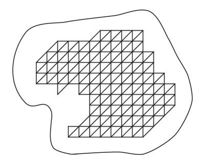
Figure 5.1: A possible simplex domain approximation for a domain $D$

Finally, for the purposes of our large deviations principles, we will need a topology—similar to the $L^{A^{*}}$ topology, for an appropriate Young function $A$—on a space which includes the functions from $\tilde{D}_{n}$ to $\mathbb{R}$ for all $n$. Suppose that $\frac{1}{n}D_{n}$ are good approximations of $D$. Let

$$L^{A^{*}}_{0}(D)=L^{A^{*}}(D)\cup_{n=1}^{\infty}L^{B}(\tilde{D}_{n}).$$

For notational convenience, we write $\tilde{D}_{\infty}=D$. Assume $A$ has Sobolev conjugate $A_{d}$ and that $A^{*}$ increases essentially more slowly than $A_{d}$ near infinity. For any $\phi_{1}$ and $\phi_{2}$ in $L^{A^{*}}_{0}(D)$ (defined on $\tilde{D}_{i}$ and $\tilde{D}_{j}$ respectively), write $\delta(\phi_{1},\phi_{2})=||\phi_{1}-\phi_{2}||_{A^{*},\tilde{D}_{i}\cap\tilde{D}_{j}}+|\tilde{D}_{i}-\tilde{D}_{j}|$, where $|\tilde{D}_{i}-\tilde{D}_{j}|$ denotes the Lebesgue measure of the symmetric difference of these two sets. We treat $L^{A^{*}}_{0}(D)$ as being endowed with the topology generated by this metric. If $\phi$ is defined on $\tilde{D}_{n}$, write $\mathcal{E}(\nabla\phi)=\int_{\tilde{D}_{n}}A(\nabla(\phi_{i}))$.

Lemma 5.2.3

The set $X_{C}$ of zero-mean functions $\phi\in L^{A^{*}}_{0}(D)$ with $\mathcal{E}(\nabla\phi)\leq C$ is compact in $L^{A^{*}}_{0}(D)$.

• Since $L^{A^{*}}_{0}(D)$ is a metric space, it is sufficient to prove that $X_{C}$ is sequentially compact. Let $\phi_{i}$ be any sequence of functions in $L^{A^{*}}_{0}(D)$; if an infinite number of the $\phi_{i}$ are defined on the same $\tilde{D}_{n}$, then the existence of a convergent subsequence follows from Lemma 5.1.3. Otherwise, we may assume that $\phi_{i}$ are defined on $\tilde{D}_{n}$ where $n$ is increasing in $i$. By a diagonalization argument, we can choose a subsequence $m(i)$ of the integers, indexed by $i$, whose restrictions to $\tilde{D}_{n}$ (which are defined when $i$ is large enough so that $\phi_{i}$ is defined on a superset of $\tilde{D}_{n}$) converge, for each $n$, to a limit in $L^{A^{*}}(\tilde{D}_{n})$ (again, by Lemma 5.1.3). Thus, there is a unique function $\phi$ such that $\phi_{m(i)}$ converges to $\phi$ on every compact subset of $D$. We need only to check that $\phi\in L^{A^{*}}(D)$ and that the $\phi_{m(i)}$ also converge to $\phi$ with respect to the metric $\delta$.

  Since there is a uniform upper bound on the isoperimetric constants of the $\tilde{D}_{n}$, by Theorem 5.1.3, there is a uniform upper bound $k$ on $||\phi_{i}||_{A^{*},\tilde{D}_{i}}$, and hence on $||\phi||_{A^{*},\tilde{D}_{n}}$ as well. If we had $\int_{D}A^{*}(\frac{\phi(\eta)}{k})d\eta>1$, then for some $i$, we would have $\int_{\tilde{D}_{i}}A^{*}(\frac{\phi(\eta)}{k})d\eta>1$, a contradiction. Hence $||\phi||_{A^{*},D}\leq k$.

  Next, we know that for ever $\epsilon$ and $n$ there exists an $N$ such that for all $m\geq N$, we have $||\phi_{m}-\phi||_{A^{*},\tilde{D}_{n}}<\epsilon$. Let $\psi^{\epsilon}_{n}=1_{D\backslash\tilde{D}_{n}}\phi_{m}-\phi$; it will be clear that $\delta(\phi_{n},\phi)\rightarrow 0$ if we can show that $||\psi^{\epsilon}_{n}||_{A^{*},D}$ tends to zero for every fixed $\epsilon$. This follows easily from the fact that $||\psi^{\epsilon}_{n}||_{A_{d},D}$ is uniformly bounded (independently of $n$), that the volume of the sets on which $\psi^{\epsilon}_{n}$ are supported is tend to zero in $n$, and that $A^{*}$ increases essentially more slowly near infinity than $A_{d}$.   

The following corollary is the only compactness result we will actually need in our proof of the large deviations principle (in the space $L^{A^{*}}_{0}(D)$) for random surfaces defined using isotropic convex nearest neighbor potentials.

Corollary 5.2.4

Let $Y_{C}$ be the set of zero-mean functions of the form $\tilde{\phi}$, where $\phi:D_{n}\mapsto\mathbb{R}$ satisfies

$$H^{o}_{D_{n}}(\phi)\leq C|D_{n}|.$$

Here $H$ is the Hamiltonian for the isoperimetric convex nearest neighbor potential determined by $A$. If $A$ has a conjugate $A_{d}$ and $A^{*}$ increases essentially more slowly than $A_{d}$, then $Y_{C}$ is precompact in $L^{A^{*}}_{0}(D)$. The same is true if $A$ does not have a conjugate but $A_{d}$ is a conjugate of a Young function equivalent to $A$.

• When $A$ has conjugate $A_{d}$, the statement follows immediately from Lemma 5.2.1 and Lemma 5.2.3. When $A$ does not have a conjugate, we can replace $A$ with an $A_{0}$ that does have a conjugate and for which $|A(\eta)-A_{0}(\eta)|\leq b$ for $\eta\in\mathbb{R}$. (See Remark 3.3 of [16].) Thus, $|D_{n}|^{-1}H^{o}_{D_{n}}(\phi)$ defined using $A$ differs only by a constant amount from the analogous expression defined using $A_{0}$. Since $D$ has finite volume, the $Y_{C}$ defined using $A$ is a subset of some $Y_{C_{0}}$, defined using $A_{0}$ in place of $A$, and the corollary follows.   

5.3 Low energy interpolations from $L^{1}$ and $L^{1,A}$ bounds

5.3.1 $L^{A}$ bounds from $L^{1}$ and $L^{1,A}$ bounds

Let $C\in\mathbb{R}$ be an arbitrary constant and let $S_{A,C}(D)$ be the set of weakly differentiable functions $f$ on $D$ with $||\nabla f||_{A}\leq C$. The following theorem states that the imbedding of $L^{1}(D)\cap S_{A,C}(D)$ (with the $L^{1}$ norm) into $L^{A}\cap S_{A,C}$ (with the $L^{A}$ norm) is continuous.

Lemma 5.3.1

Let $A$ be a Young function and $D\in\mathbb{G}(\frac{d-1}{d})$ and $C>0$. For every $\epsilon$, there exists a $\delta=\delta(C,\epsilon,A)>0$ such that the following two conditions

1. $||\nabla f||_{A}\leq C$

2. $||f||_{1}\leq\delta$

together imply $||f||_{A}\leq\epsilon$. The lemma remains true if we replace the first statement with the modified statement: $\int_{D}A(\nabla f(\eta))d\eta\leq C$.

• First of all, if $||\nabla f||_{A}\leq C$, then $g=f/C$ satisfies $\int_{D}(\nabla f(\eta))d\eta\leq 1$—i.e., $g$ satisfies the modified statement with $C=1$. It will therefore be enough to show that the modified first statement and the second statement together imply the conclusion. Statements $2.21$ (and subsequent discussion) and $2.25$ of [16] indicate that for some constant $K$ (depending only on $D$ and $A$), we have $||\nabla f||_{A}\geq||K\nabla f^{*}||_{A}$ whenever $f^{*}$ is a positive, radially decreasing, spherically symmetric “rearrangement” of $f$ defined on a sphere $D^{\prime}$ with the same volume as $D$. Though we do not define rearrangements precisely here, it suffices to note that such rearrangements always exist for measurable $f$, and whenever $f^{*}$ is a rearrangement of $f$, we have $||f||_{A}=||f^{*}||_{A}$ and $||f||_{1}=||f^{*}||_{1}$ and $\int_{D}A(|\nabla f(\eta)|)d\eta=\int_{D^{\prime}}A(|\nabla f^{*}(\eta)|)d\eta$. Thus, if $f$ violates the theorem conclusion for a particular choice of $C$, $\delta$, and $\epsilon$, then $f^{*}$ violates the statement for the same values.

  It is therefore sufficient to prove the result for positive, radially decreasing spherically symmetric functions $f(\eta)=g(|\eta|)$—defined on a sphere $D^{\prime}$ of radius $R$) with $g:(0,R]\mapsto[0,\infty)$ decreasing. Thus, the theorem is implied by (the $K=1$ case of) the following assertion: For every $\epsilon>0$ and $K>0$ and $C>0$ there exists a $\delta>0$ such that

  1. $\int_{0}^{R}\left(A(|g^{\prime}(r)|)d\Gamma_{d}r^{d-1}\right)dr\leq C$

  2. $\int_{0}^{R}\left(|g(r)|d\Gamma_{d}r^{d-1}\right)dr\leq\delta$

  together imply $\int_{0}^{R}\left(A\left(\frac{g(r)}{\epsilon}\right)d\Gamma_{d}r^{d-1}\right)dr\leq K$.

  Here $\Gamma_{d}$ is the volume of the unit sphere of radius $1$ in $d$ dimensions (and $d\Gamma_{d}$ the $n-1$-dimensional volume of its boundary). Replacing $C$, $\delta$, and $K$ with their values divided by $d\Gamma_{d}$, we eliminate that constant: it is now enough for us to prove that for any $\epsilon>0$, $C>0$, and $K>0$ there exists $\delta>0$ such that

  1. $\int_{0}^{R}A(|g^{\prime}(r)|)r^{d-1}dr\leq C$

  2. $\int_{0}^{R}|g(r)|r^{d-1}dr\leq\delta$

  together imply $\int_{0}^{R}A\left(\frac{g(r)}{\epsilon}\right)r^{d-1}dr\leq K$.

  We say the theorem “holds for $(R,C,K,\epsilon)$”, if for those fixed values, the above implication is true for some sufficiently small $\delta$. Let $\alpha>0$ and $\beta>0$ be arbitrary constants. We now show that to prove that the theorem holds for all positive $(R,C,K,\epsilon)$, it is sufficient to prove that the theorem holds for all positive $(R,C,K,\epsilon)$ for which $R\leq\alpha$; furthermore, it is enough to prove the implication for the positive, decreasing functions $g$ on $(0,R]$ for which $|g(R)|\leq\beta$. To just these two reductions, first suppose $R>\alpha$ but $0<R^{\prime}<\alpha$. Since $g$ is decreasing, we have $|g(r)|\leq|g(R^{\prime})|$ for $r>R^{\prime}$ and $\delta\geq\int_{0}^{R}|g(r)|r^{d-1}dr\geq(R^{\prime})^{d}g(R^{\prime})$. We conclude that for any fixed value of $R^{\prime}$, we can assume (when $\delta$ is small enough) that $g(R^{\prime})\leq\beta$. Moreover,

  $$\int_{R^{\prime}}^{R}A\left(\frac{g(r)}{\epsilon}\right)r^{d-1}dr\leq\int_{R^{\prime}}^{R}A\left(\frac{\delta}{(R^{\prime})^{d}}\right).$$

  For fixed $R^{\prime}$, $R$, and $A$, the latter term clearly tends to zero as $\delta$ tends to zero. Thus, it is enough for us to bound $\int_{0}^{R^{\prime}}A(\frac{g(r)}{\epsilon})r^{d-1}dr$; and we can do this by solving the modified problem with $R=R^{\prime}<\alpha$.

  Thus, we may assume $R\leq\frac{\epsilon}{2}$ throughout the remainder of the proof. Now, putting $t=R-r$, and noting $\frac{t}{\epsilon}\leq\frac{1}{2}$ (since $R\leq\frac{\epsilon}{2}$), we can write

  $$\frac{g(r)}{\epsilon}=\frac{g(R)}{\epsilon}+\frac{1}{\epsilon}\int_{r}^{R}|g^{\prime}(u)|du=\left(1-\frac{t}{\epsilon}\right)\frac{g(R)}{\epsilon\left(1-\frac{t}{\epsilon}\right)}+\frac{t}{\epsilon}\int_{r}^{R}|g^{\prime}(u)|d(u/t).$$

  Applying Jensen’s inequality repeatedly (see explanation below), we conclude that

  $$A\left(\frac{g(r)}{\epsilon}\right)\leq\left(1-\frac{t}{\epsilon}\right)A\left(\frac{g(R)}{\epsilon\left(1-\frac{t}{\epsilon}\right)}\right)+\frac{t}{\epsilon}A\left(\int_{r}^{R}|g^{\prime}(u)|d(u/t)\right)\leq$$

  $$A\left(\frac{g(R)}{\epsilon}\right)+\frac{1}{\epsilon}\int_{r}^{R}A(|g^{\prime}(u)|)du.$$

  The second inequality uses the fact that $A$ is convex and $A(0)=0$ along with the bound $\frac{t}{\epsilon}<1/2$ for the first term and a second application of Jensen’s inequality to the probability measure $d(u/t)$ on $(r,R)$ for the second term. We conclude that

  $$A\left(\frac{g(r)}{\epsilon}\right)\leq A\left(\frac{g(R)}{\epsilon}\right)+\frac{1}{\epsilon}\int_{r}^{R}A(|g^{\prime}(u)|)du.$$

  Now we integrate both sides of the inequality, using Fubini’s theorem on the second term of the right hand side to change order of integration. We then get the result

  $$\int_{0}^{R}A\left(\frac{g(r)}{\epsilon}\right)r^{d-1}dr\leq\int_{0}^{R}r^{d-1}A\left(\frac{g(R)}{\epsilon}\right)dr+\frac{1}{\epsilon}\int_{0}^{R}\int_{r}^{R}r^{d-1}A\left(|g^{\prime}(u)|\right)dudr=$$

  $$A\left(\frac{g(R)}{\epsilon}\right)\frac{R^{d}}{d}+\frac{1}{\epsilon}\int_{0}^{R}\int_{0}^{u}r^{d-1}A\left(|g^{\prime}(u)|\right)drdu=$$

  $$A\left(\frac{g(R)}{\epsilon}\right)\frac{R^{d}}{d}+\frac{1}{\epsilon}\int_{0}^{R}\frac{u^{d}}{d}A(|g^{\prime}(u)|)du.$$

  Since $u^{d}<Ru^{d-1}$ we have the bound (from the modified first assumption in the lemma statement)

  $$\int_{0}^{R}A\left(\frac{g(r)}{\epsilon}\right)r^{d-1}dr\leq A\left(\frac{g(R)}{\epsilon}\right)\frac{R^{d}}{d}+\frac{CR}{\epsilon}.$$

  For any fixed $A$, $\epsilon$, and $C$, we can assume $\alpha$ and $\beta$ are small enough so that the latter expression is less than one (since $R\leq\alpha$ and $g(R)\leq\beta$).   

5.3.2 Interpolations from $d-1$-dimensional $L^{1}$ and $L^{1,A}$ bounds

Let $G\subset\mathbb{R}^{d-1}$ be the $d-1$-dimensional unit cube. Suppose we are given a linear function $f_{u}:\mathbb{R}^{d}\mapsto\mathbb{R}$ defined by $f_{u}(\eta)=(u,\eta)$ (where $u\in\mathbb{R}^{d}$), and a function $f$ defined on $G$.

For any $\epsilon$, we can construct an interpolation between $f_{u}$ and $f$ on $G\times[0,\epsilon]$ as follows. Then write

$$g(\eta)=\frac{\eta_{n}}{\epsilon}f_{u}(\eta_{1},\eta_{2},\ldots,\eta_{n-1},\epsilon)+\frac{\epsilon-\eta_{n}}{\epsilon}f(\eta_{1},\eta_{2},\ldots,\eta_{n-1}).$$

The following lemma implies that, under appropriate conditions, we can make $\epsilon$ small and still maintain an upper bound on the “average energy” of the interpolation function $g$ over $G\times[0,\epsilon]$.

Lemma 5.3.2

Fix a constant $C>0$. For every $\epsilon>0$, there exists a $\delta>0$ so that the following three statements

1. $A(u)\leq C$

2. $\int_{G}A(\nabla f(\eta))d\eta\leq C$

3. $||h(\eta)||_{1}\leq\delta$, where $h(\eta)=f_{u}(\eta_{1},\ldots,\eta_{n-1},0)-f(\eta_{1},\ldots,\eta_{n-1})$

together imply that $\frac{1}{\epsilon}\int_{[G\times\epsilon]}A(g(\eta))d\eta\leq 4C$.

• If $g_{\eta_{1}},\ldots,g_{\eta_{d}}$ are the partial derivatives of $g$, we can write

  $$\frac{1}{\epsilon}\int_{G\times[0,\epsilon]}A(\nabla g(\eta))d\eta=\sum_{i=1}^{d}\frac{1}{\epsilon}\int_{G\times[0,\epsilon]}A(\nabla g_{\eta_{i}}(\eta))d\eta.$$

  Since the first $d-1$ derivatives are weighted averages of derivatives of $f$ and $f_{u}$, the sum of the first $d-1$ terms is bounded by $\int_{G}A(\nabla f(\eta))d\eta+\sum_{i=1}^{d-1}A(u_{i})\leq C+C=2C$. The $d$th term is given by

  $$\int_{G}A\left(\frac{f_{u}(\eta_{1},\ldots,\eta_{n-1},\epsilon)-f(\eta_{1},\ldots,\eta_{n-1})}{\epsilon}\right)d\eta=\int_{G}A\left(\frac{h(\eta)}{\epsilon}+u_{n}\right)d\eta.$$

  Write $B(\eta)=\frac{A(\eta)}{2C}$. For any $\delta_{0}>0$, Lemma 5.3.1 implies that for $\delta$ small enough we have $||f||_{B}\leq\delta_{0}$. Note that $||u_{n}||_{B,G}\leq 1/2$ (where $u=(u_{1},\ldots,u_{n})$, and we treat $u_{n}$ as a constant function). If $\delta_{0}$ is small enough so that $||\frac{h}{\epsilon}||_{B,G}\leq\frac{1}{2}$, then $||\frac{h}{\epsilon}+u_{n}||_{B}\leq 1$ and hence $\int_{G}A\left(\frac{h(\eta)}{\epsilon}+u_{n}\right)d\eta\leq 2C$.   

Now, suppose that $G_{1},\ldots,G_{2d}$ are the $2d$ faces of the $d$-dimensional unit cube $D\subset\mathbb{R}^{d}$ and fix some $\epsilon<1/2$. Let $D_{\epsilon}$ be the cube of side length $1-2\epsilon$, positioned in $\mathbb{R}^{d}$ so as to be concentric with $D$. Given $f:D\mapsto\mathbb{R}$, we can interpolate between $f$ and $f_{u}$ as follows.

For $1\leq\leq 2d$, let $G_{i}^{\prime}$ be the face obtained by shifting $G_{i}$ by $\epsilon$ units in a perpendicular direction, so that it borders $D^{\prime}$. Let $g_{i}$ be the linear interpolation between between $f$ (on $G_{i}$) and $f_{u}$ (on $G_{i}^{\prime}$), similar to the linear interpolation on $G\times[0,\epsilon]$ described above; we can extend $g_{i}$ to all of $D$ by writing $g_{i}(\eta)=f_{u}(\eta)$ whenever $\eta$ and $G_{i}$ are on opposite sides of $G_{i}^{\prime}$.

Now, we define an inner interpolation function

$$g_{I}(\eta)=\begin{cases}\inf_{1\leq i\leq 2d}\{g_{i}(\eta)\},&f(\eta)\leq\inf_{1\leq i\leq 2d}g_{i}(\eta)\\ \sup_{1\leq i\leq 2d}\{g_{i}(\eta)\},&f(\eta)\geq\sup_{1\leq i\leq 2d}g_{i}(\eta)\\ f(\eta),&\text{otherwise.}\\ \end{cases}$$

Since $f(\eta)=g_{i}(\eta)$, for some $i$, for all $\eta$ on the boundary of $D$, we have $g(\eta)=f(\eta)$ on the boundary of $D$. Moreover, since all of the $g_{i}$’s are equal to $f_{u}$ inside $D^{\prime}$, we have $g(\eta)=f_{u}(\eta)$ for $\eta\in D^{\prime}$. Similarly, we define an outer interpolation function by letting $g_{i}^{\prime}$ be the interpolation between $f_{u}$ (on $G_{i}$) and $f$ (on $G_{i}^{\prime}$ and the portion of $D$ that lies on the opposite side of $G_{i}^{\prime}$ from $G_{i}$). Then

$$g_{O}(\eta)=\begin{cases}\inf_{1\leq i\leq 2d}\{g_{i}(\eta)\},&f_{u}(\eta)\leq\inf_{1\leq i\leq 2d}g_{i}(\eta)\\ \sup_{1\leq i\leq 2d}\{g_{i}(\eta)\},&f_{u}(\eta)\geq\sup_{1\leq i\leq 2d}g_{i}(\eta)\\ f_{u}(\eta),&\text{otherwise.}\\ \end{cases}$$

This $g_{O}(\eta)$ is equal to $f_{u}(\eta)$ on the boundary of $D$ and $f(\eta)$ inside of $D^{\prime}$. The following lemma gives energy bounds on $g_{O}(\eta)$ and $g_{I}(\eta)$.

Lemma 5.3.3

Let $G$ be the outer surface of a unit cube $D\subset\mathbb{R}^{d}$. Fix a constant $C>0$. For every $\epsilon>0$, there exists a $\delta>0$ for which the following four statements

1. $A(u)\leq C$

2. $\int_{D\backslash D^{\prime}}A(\nabla f(\eta))d\eta\leq C|D\backslash D^{\prime}|$

3. $\int_{\partial D}A(\nabla(f(\eta))d\eta$ is well defined as a $d-1$-dimensional integral and is less than or equal to $2dC$

4. $||f-f_{u}||_{1,\partial D}\delta$

together imply

$$|D\backslash D^{\prime}|^{-1}\int_{D\backslash D^{\prime}}A(g_{I}(\eta))d\eta\leq(4C)(2d+1)=8dC+4C$$

and the analogous statement for $g_{O}$.

• The main observation is that $\nabla g_{I}(\eta)\leq\max\{f(\eta),\nabla g_{1}(\eta),\nabla g_{2}(\eta),\ldots,\nabla g_{2d}(\eta)\}$ for almost all $\eta$ (and the same is true for $g_{O}$). Arguments similar to Lemma produce a bound of $4C$ on $|D\backslash D^{\prime}|^{-1}\int_{D\backslash D^{\prime}}A(g_{i}(\eta))d\eta$ for each $i$, and the result follows.   

We can actually derive a similar version of the above lemma in which the bound on $\int_{\partial D}A(\nabla(f(\eta))d\eta$ is omitted. Define $g_{I}^{\gamma,\epsilon}$ as follows. First, for some $0<\gamma<1$, we define $f_{\gamma}D\mapsto\mathbb{R}$ by $f_{\gamma}(\eta)=\frac{1}{\gamma}f(\gamma\eta)$. (Assume here that $D$ is centered at the origin; so $f_{\gamma}$ is essentially “zooming in” on the portion of $f$ defined on the cube $D_{\gamma}$ of side length $\gamma$ that is concentric with $D$.) The construct the interpolations $g_{I}$ and $g_{O}$ (as described above) using $f_{\gamma}$ instead of $f$. Then we “zoom back out” by writing

$$g_{I}^{\gamma,\epsilon}(\eta)=\begin{cases}\gamma g_{I}\left(\frac{\eta}{\gamma}\right)&\eta\in D_{\gamma}\\ f(\eta)&\text{otherwise.}\\ \end{cases}$$

Now we have:

Lemma 5.3.4

Let $D$ be the unit cube. There exists a constant $C_{0}>0$ for which the following is true. Fix a constant $C>0$. For all sufficiently small $\epsilon>0$, there exists a $\delta>0$ for which the following three statements

1. $A(u)\leq C$

2. $\int_{D}|D|^{-1}A(\nabla f(\eta))d\eta\leq C$

3. $||f-f_{u}||_{1,D}\leq\delta$

together imply that for some $\gamma$ with $1-\epsilon<\gamma<1$,

$$\int_{D\backslash D_{1-2\epsilon}}A(g_{I}^{\gamma,\epsilon}(\eta))d\eta\leq C_{0}C|D\backslash D_{1-2\epsilon}|.$$

In particular, the average value of $A(\nabla g_{I}^{\gamma,\epsilon})$, over the region where it fails to be equal to $f_{u}$, is bounded above by $C_{0}C$. A similar statement is true for $g_{O}^{\gamma,\epsilon}$, where the roles of $f_{u}$ and $f$ are reversed. Also, the conclusion of the lemma remains true if we replace $D$ by $\frac{1}{n}D$, provided we $\delta$ with $\frac{\delta}{n^{-d-1}}$.

• Since $\int_{D}A(\nabla f(\eta))d\eta\leq C$, then we must have $\int_{\partial D_{\gamma}}A(\nabla(f(\eta))d\eta\leq 2C/\epsilon$ for a set of $\gamma$ values in $[1-\epsilon,1]$ with measure at least $\epsilon/2$. Since $||f-f_{u}||_{1}\leq\delta$, then we must have

  $$\int_{\partial D_{\gamma}}||f-f_{u}||_{1}\leq 2\delta/\epsilon$$

  for at least one of the $\gamma$ values for which $\int_{\partial D_{\gamma}}A(\nabla(f(\eta))d\eta\leq 2C/\epsilon$. For $\epsilon$ sufficiently small, the volume of $D_{\gamma}\backslash D_{\gamma(1-\epsilon)}$ is bounded above by $3d\epsilon$. The result then follows by applying Lemma 5.3.3 to $f_{\gamma}$ (as defined above). The argument for $g_{O}^{\gamma,\epsilon}$ is similar. The analogous statement for $\frac{1}{n}D$ follows immediately from the rescaling $f_{n}:\frac{1}{n}D\mapsto\mathbb{R}$ given by $f_{n}(\eta)=\frac{1}{n}f(n\eta)$.   

5.3.3 Discrete interpolation lemma

The proof of the following discrete analog of Lemma 5.3.4 is virtually identical to the proof of its continuous counterpart. Let $\Delta_{n}=[0,n]^{d}-v$, where $v\in\mathbb{Z}^{d}$ is the vector with all components equal to $\lfloor n/2\rfloor$. If $a\not\in\mathbb{Z}$, write $\Delta_{a}=\Delta_{\lfloor a\rfloor}$.

Lemma 5.3.5

Fix a constant $C>0$. There exists a constant $C_{0}$ such that the following is true: For all sufficiently small $\epsilon>0$, there exists a $\delta>0$ such that for all sufficiently large $n$ and any $\phi:\Delta_{n}\mapsto\mathbb{R}$, the following three statements

1. $A(u)\leq C$

2. $H^{o}_{\Delta_{n}}(\phi)\leq C|\Delta_{n}|$ (where $\Phi$ has nearest neighbor gradient potentials determined by $A$)

3. $\sum_{x\in\Delta_{n}}|\phi(x)-(x,u)|\leq\delta|\Delta_{n}|$

together imply that there exists an inside interpolation function $\psi_{I}$ for which

1. $\psi_{I}(x)=\phi(x)$ for all $x\in\partial\Delta_{n}$.

2. $\psi_{I}(x)=(u,x)$ for all $x$ contained in $\Delta_{(1-\epsilon)n}$.

3. $H^{\overline{\Phi}}_{\Delta_{n}\backslash\Lambda_{(1-\epsilon)n}}(\psi_{I})\leq C_{0}C\epsilon n^{d}$.

The same criteria imply the existence of an outside interpolation function $\psi_{O}:\Delta_{n}\mapsto\mathbb{R}$ for which

1. $\psi_{O}(x)=(u,x)$ for all $x\in\partial\Delta_{n}$.

2. $\psi_{O}(x)=\phi(x)$ for all $x$ contained in $\Delta_{(1-\epsilon)n}$.

3. $H^{\overline{\Phi}}_{\Delta_{n}\backslash\Delta_{(1-\epsilon)n}}(\psi_{O})\leq C_{0}C\epsilon n^{d}$.

5.4 Approximation by “mostly linear” functions

In this section, we will see that every $f\in L^{1,A}(D)$ can be approximated by a function which “mostly agrees” with one of the linear approximators $F_{n}$ (defined in the following lemma) and whose total energy outside of the areas on which it agrees with $F_{n}$ is small. This construction will be useful to us in Chapter 7.

Lemma 5.4.1

Fix $f\in L^{1,1}(D)$. Let $F_{n}(\eta)$ be the piecewise linear (linear on simplices) function (not continuous in general) whose mean and mean gradient are equal to those of $f$ on each simplex of $\frac{1}{n}\mathbb{Z}^{d}$. Then

$$\lim_{n\rightarrow\infty}||\nabla f-\nabla F_{n}||_{1}=0.$$

• This merely says $\nabla f$ can be approximated by step functions.   

Lemma 5.4.2

For any $f\in L^{1,1}(D)$, $||f-F_{n}||_{1}=o(\frac{1}{n})$.

• This follows from applying Lemma 5.4.1 and Theorem 5.1.3 to $f-F_{n}$.   

Lemma 5.4.3

Suppose $f\in L^{1,A}(D)$ and fix $\epsilon>0$. Then for all $n$ sufficiently large, there exists a function $F_{\epsilon}\in L^{1,A}(D)$ that is equal to $F_{n}$ on a closed subset $D^{\prime}$ of $D$, where the volume of $D\backslash D^{\prime}$ is less than $\epsilon$ and $\int_{D-D^{\prime}}A(\nabla F_{\epsilon})\leq\epsilon$.

• First, for any $\epsilon_{0}>0$, choose $C\geq 2\frac{\int_{D}A(\nabla f(\eta))d\eta}{\epsilon_{0}}$. For any $\delta>0$, the fraction of boxes $b$ (of side length $1/n$) that satisfy $||f-F_{n}||_{1,b}\leq\frac{\delta}{n^{d+1}}$ tends to zero in $n$. It follows that for sufficiently large $n$ and any $\delta$, the three conditions of Lemma 5.3.4 will apply to at least a $1-\epsilon_{0}$ fraction of the boxes of the mesh $\frac{1}{n}\mathbb{Z}^{d}$. We can now define our interpolation function $F_{\epsilon}$ to be equal to $f$ on the boxes for which the conditions of Lemma 5.3.4 do not apply and equal to the interpolation described by Lemma 5.3.4 on the boxes on which they do apply. It is clear from the lemma that if we take a sufficiently small $\epsilon_{0}<\epsilon$, we can also arrange to have $\int_{D-D^{\prime}}A(\nabla F_{\epsilon})\leq\epsilon$.   

In Chapter 7, given a function $f$ defined on $D$, and good approximation $D_{n}$ of $f$, we will sometimes use a very naive approach (described in the following lemma) for defining functions $\phi_{n}:D_{n}\mapsto\mathbb{R}$ which (appropriately rescaled) approximate $f$.

Lemma 5.4.4

Fix: $f:D\mapsto\mathbb{R}$ and suppose that $\int_{D}A(\nabla f(\eta))d\eta$ is finite. Let the sequence $D_{n}$ be a good approximation of $D$. Then the sequence of functions $\phi_{n}:D_{n}\mapsto\mathbb{R}$ (approximating $f$) defined by $\phi_{n}(y)=n^{d+1}\int_{\{\eta:\lfloor n\eta\rfloor=y\}}f(\eta)d\eta$ satisfies $|D_{n}|^{-1}H^{o}_{D_{n}}(\phi_{n})\leq C_{0}\int_{D}A(\nabla f(\eta))d\eta$ for some $C_{0}$ independent of $n$ and $f$.

• Write $s_{n}(\eta)$ for the cube $\{\eta:\lfloor n\eta\rfloor=y\}$. Because $D_{n}$ is a good approximation, all of the cubes $s_{n}(\eta)$, for $\eta\in D_{n}$, are subsets of $D$. Note further that

  $$\phi_{n}(\eta)-\phi_{n}(\eta+e_{i})=n^{d+1}\int_{s_{n}(\eta)}\int_{t=0}^{\frac{1}{n}}\frac{\partial}{\partial\eta_{i}}f(\eta+te_{i}))dtd\eta.$$

  By Jensen’s inequality (and the fact that $n^{d+1}\int_{s_{n}(\eta)}\int_{0}^{1/n}dtd\eta=1$), we have

  $$A(\phi_{n}(\eta)-\phi_{n}(\eta+e_{i}))\leq n^{d+1}\int_{s_{n}(\eta)}\int_{t=0}^{\frac{1}{n}}A\left(\frac{\partial}{\partial\eta_{i}}f(\eta)\right)d\eta.$$

  The result follows by summing these integrals over all edges of $D_{n}$.   

Chapter 6 Limit equalities and the variational principle

The first goal of this chapter is to derive some equivalent definitions of specific free energy (making use of the notion of “empirical measure” of a configuration $\phi:\Lambda_{n}\mapsto E$) and an equivalent definition of the surface tension. In Section 6.1, we prove the equivalence of these definitions in the simplest setting: when $\Phi$ is an SAP and $(E,\mathcal{E})$ is $\mathbb{R}$, endowed with the Borel $\sigma$-algebra. In Section 6.2, we describe some (relatively minor) technical modifications to the arguments of Section 6.1 that enable us to extend these results to all perturbed SAPs, as well as to higher dimensional real and discrete models ($E=\mathbb{R}^{m}$ or $E=\mathbb{Z}^{m}$).

The second goal of the chapter is to prove the second half of the variational principle—namely, that every $\mathcal{L}$-invariant gradient phase $\mu$ of slope $u\in U_{\Phi}$ has minimal specific free energy among $\mathcal{L}$-invariant measures of slope $u$ and hence satisfies $SFE(\mu)=\sigma(u)$. In Section 6.3 we prove this when $\Phi=\Phi_{V}$ is an ISAP and $(E,\mathcal{E})$ is $\mathbb{R}$, endowed with the Borel $\sigma$-algebra. In Section 6.4, we describe the (again, relatively minor) technical modifications to the arguments of Section 6.3 that enable us to extend them, for $E=\mathbb{R}^{m}$ or $E=\mathbb{Z}^{m}$, to all perturbed ISAP’s and perturbed LSAP’s. (It is not known whether the second half of the variational principle—like the first half—holds for all perturbed SAPs.)

6.1 Limit equalities: $PBL(\mu)$, $FBL(\mu)$, and $SFE(\mu)$

Throughout this section, we will assume that $E=\mathbb{R}$ and $\Phi$ is an SAP. Denote by $\mathcal{A}$ the topology of local convergence on $\mathcal{P}(\Omega,\mathcal{F}^{\tau})$ and by $\mathcal{B}$ the basis for that topology consisting of finite intersections of sets of the form $\{\mu:\mu(F)<\epsilon\}$ where $0<\epsilon<1$ and $F:\Omega\rightarrow\mathbb{R}$ is $\mathcal{F}_{\Lambda}^{\tau}$-measurable for some $\Lambda\subset\subset\mathbb{Z}^{d}$, and $F$ is bounded between $0$ and $1$.

For notational convenience, throughout the following two chapters, we will also augment the space $\Omega$ to be the space of functions from $\mathbb{Z}^{d}$ to $\mathbb{R}\cup\{\infty\}$ instead of merely from $\mathbb{Z}^{d}$ to $\mathbb{R}$. Whenever we deal with a real-valued function $\phi$ that we have defined only on a subset $\Lambda$ of $\mathbb{Z}^{d}$, we tacitly assume that it extends to a function in $\Omega$ for which $\phi(x)=\infty$ for $x\not\in\Lambda$. (So in this context, the statement $\phi(x)=\infty$ is a way of saying that $\phi(x)$ has not been defined.)

Given $u\in\mathbb{R}^{d}$, let $\phi_{u}:\mathbb{Z}^{d}\mapsto\mathbb{R}$ be a function with an $\mathcal{L}$-periodic gradient and $\epsilon$ a positive constant for which

1. $\phi_{u}$ has asymptotic slope given by $u$.

2. There exists a finite constant $C$ such that for any edge $(x,y)$ in $\mathbb{Z}^{d}$ and any $\phi$ bounded between $\phi_{u}-2\epsilon$ and $\phi_{u}+2\epsilon$, we have: $V_{x,y}(\phi(y)-\phi(x))\leq C$.

Arguments similar to those in Lemma 4.2.2 and Lemma 4.3.2 imply that—whenever $\Phi$ is an SAP and $u\in U_{\Phi}$—there exists at least one such pair $(\phi_{u},\epsilon)$. As in previous chapters, we take $\Lambda_{n}=[0,kn-1]^{d}$ where $k$ is chosen so that $k\mathbb{Z}^{d}\subset\mathcal{L}$. Let $C^{u}_{n}$ be the subset of maps $\phi:\Lambda_{n}\mapsto\mathbb{R}$ for which $|[\phi(x)-\phi(x_{0})]-[\phi_{u}(x)-\phi_{u}(x_{0})]|\leq\epsilon$ for all $x\in\partial\Lambda_{n}\backslash\{x_{0}\}$. (Here, $x_{0}$ is the origin, so it lies on one corner of the boundary of $\Lambda_{n}=[0,kn-1]^{d}$.) The functions in $C^{u}_{n}$ are those functions which (up to additive constant) closely approximate the periodic function $\phi_{u}$ on the boundary of $\Lambda_{n}$.

Given a $B\in\mathcal{B}$, let $B_{n}$ be the set of functions $\phi:\Lambda_{n}\mapsto\mathbb{R}$ whose empirical measures lie in $B$. To say this precisely, let $\theta_{x}$ denote translation by $x\in\mathcal{L}$. Define $L_{n}(\phi)$, a measure on $(\Omega,\mathcal{F})$, by

$$L_{n}(\phi)=|\Lambda_{n}\cap\mathcal{L}|^{-1}\sum_{x\in\Lambda_{n}\cap\mathcal{L}}\delta_{\theta_{x}\phi}.$$

Then write $B_{n}=\{\phi|L_{n}(\phi)\in B\}$. In the following definitions, we will assume that $u\in U$ and that $\phi_{u}$ and $\epsilon$ are fixed. After we prove Theorem 6.1.1, it will be clear that the definition of $PBL$ is independent of the particular choice of $\phi_{u}$ and $\epsilon$. We use the initials $PBL$ to mean “pinned boundary limit” and write

$$PBL^{u}_{B}(\mu)=\limsup_{n\rightarrow\infty}-|\Lambda_{n}|^{-1}\log\left(\int 1_{C^{u}_{n}\cap B_{n}}e^{-H^{o}_{\Lambda}(\phi)}\prod_{x\in\Lambda_{n}\backslash\{x_{0}\}}d\phi(x)\right).$$

In the integrals in the above limiting sequence, we assume $\phi(x_{0})$ is set to $0$ and $\phi(x)=\infty$ for $x\not\in\Lambda_{n}$. We also write

$$PBL^{u}(\mu)=\sup_{B\ni\mu,B\in\mathcal{B}}PBL^{u}_{B}(\mu)$$

$$PBL(\mu)=PBL^{S(\mu)}(\mu).$$

If $u\not\in U$, then write $PBL^{u}(\mu)=\infty$; in particular, if $S(\mu)\not\in U$, then $PBL(\mu)=\infty$. We now define the “free boundary limit” as follows:

$$FBL_{B}(\mu)=\liminf_{n\rightarrow\infty}-|\Lambda_{n}|^{-1}\log\left(\int 1_{B_{n}}e^{-H^{o}_{\Lambda}(\phi)}\prod_{x\in\Lambda_{n}\backslash\{x_{0}\}}d\phi(x)\right)$$

$$FBL(\mu)=\sup_{B\ni\mu,B\in\mathcal{B}}FBL_{B}(\mu)$$

Theorem 6.1.1

If $\Phi$ is an SAP, $E=\mathbb{R}$, and $\mu\in\mathcal{P}_{\mathcal{L}}(\Omega,\mathcal{F}^{\tau})$, then

$$SFE(\mu)=FBL(\mu)=PBL(\mu).$$

It is obvious that $FBL(\mu)\leq PBL^{u}(\mu)$ for any $u$; in particular $FBL(\mu)\leq PBL(\mu)$. In the following three subsections, we will prove Theorem 6.1.1 in three steps:

1. $PBL(\mu)\leq SFE(\mu)$ when $\mu$ is ergodic

2. $PBL(\mu)\leq SFE(\mu)$ for any $\mu$

3. $SFE(\mu)\leq FBL(\mu)$

6.1.1 $PBL(\mu)\leq SFE(\mu)$ for $\mu$ ergodic

First, as a simple consequence of the ergodic theorem, we show that if the gradient of $\phi$ is chosen from an $\mathcal{L}$-ergodic gradient measure $\mu$ with finite slope, then $\phi$ closely approximates a plane, in an $L^{1}$ sense, with high probability. Precisely, we show the following:

Lemma 6.1.2

Let $\mu\in\mathcal{P}_{\mathcal{L}}(\Omega,\mathcal{F}^{\tau})$ be $\mathcal{L}$-ergodic with finite slope $u\in\mathbb{R}^{d}$. Then for any fixed $\epsilon$, we have

$$\lim_{n\rightarrow\infty}\mu\{|\Lambda_{n}|^{-1}\sum_{x\in\Lambda_{n}}|\phi(x)-(x,u)-\phi_{\Lambda_{n}}|\geq\epsilon n^{d+1}\}=0,$$

where $\phi_{\Lambda_{n}}$ is the mean value of $\phi(x)-(x,u)$ on $\Lambda_{n}$.

• First, we may assume without loss of generality that when $\phi$ is chosen (defined up to additive constant) from $\mu$, we have $u=0$ and $\mu(\phi(y)-\phi(x))=0$ for each $x,y\in\mathbb{Z}^{d}$. If this is not the case, we can let $f$ be a function (determined from $\mu$ up to additive constant) for which $f(y)-f(x)=\mu(\phi(y)-\phi(x))$ for each $x,y\in\mathbb{Z}^{d}$, and then replace $\mu$ by $\mu-f$. Thus, we need only show in this case that for $\epsilon>0$, we have

  $$\lim_{n\rightarrow\infty}\mu\{|\Lambda_{n}|^{-1}\sum_{x\in\Lambda_{n}}|\phi(x)-\phi_{\Lambda_{n}}|\geq\epsilon n^{d+1}\}=0,$$

  where $\phi_{\Lambda_{n}}$ is the mean value of $\phi$ on $\Lambda_{n}$.

  When $\phi$ is chosen from $\mu$, the classical ergodic theorem (see, e.g., Chapter 14 of [43]) states that for any $\gamma>0$

  $$\lim_{n\rightarrow\infty}\mu\{|\frac{\sum_{x\in\Lambda_{n},|x-y|=1}\nabla\phi(x)}{|\Lambda_{n}|}|\geq\gamma\}=0.$$

  A trivial corollary of the ergodic theorem states that if $h:D\rightarrow\mathbb{R}^{d}$ is any continuous, bounded function on the unit cube $D$, then

  $$\lim_{n\rightarrow\infty}\mu\{|\frac{\sum_{x\in\Lambda_{n},|x-y|=1}(\nabla\phi(x),h(x/n))}{|\Lambda_{n}|}|\geq\gamma\}=0.$$

  Now, write $\Delta_{n}=(nk)e_{1}+\Lambda_{n}$, where $e_{1}$ is a basis vector of $\mathbb{Z}^{d}$. So $\Delta_{n}$ and $\Lambda_{n}$ are adjacent blocks. A discrete integration by parts gives

  $$\sum_{y\in\Delta_{n}}\phi(y)-\sum_{x\in\Lambda_{n}}\phi(x)=(nk)^{d+1}\sum_{x\in\Delta_{n}\cup\Lambda_{n}}[\phi(x)-\phi(x-e_{1})]h(x/n),$$

  where $h(v)=v_{1}$ for $v=(v_{1},\ldots,v_{d})\in D$ and $h(v)=2-v_{1}$ for $v\in D+e_{1}$. It follows that for any $\gamma$, the probability that the mean value of $\phi$ on $\Lambda_{n}$ differs from the mean value on $\Delta_{n}$ by more than $\gamma n^{d+1}$ tends to zero in $n$.

  Similarly, if we take a large integer $c$ and form a $(ckn)^{d}$ cube by joining $c^{d}$ translated $\Lambda_{n}$ blocks, then for any fixed $\gamma$, the probability that the mean value on any one of these blocks differs from the value on any other by $\gamma n^{d+1}$ will tend to zero in $n$.

  Let $C$ be supremum of $\mu(|\nabla\phi(x)|)$ for $x\in\mathbb{Z}^{d}$. The probability that the mean value of $|\nabla(\phi)|$ on one of these blocks is greater than $2C$ also tends to zero in $n$. It follows from the first part of Theorem 5.1.3 and Corollary 5.2.2 that for some $C_{0}$ (independent of $\delta$) we have, for any $\delta_{0}$,

  $$\lim_{n\rightarrow\infty}\mu\{|\Lambda_{n}|^{-1}\sum_{x\in\Lambda_{n}}|\phi(x)-\phi_{\Lambda_{n}}|\geq C_{0}n^{d+1}\}=0.$$

  Now, taking $N=cn$, the above claims imply that (when $N$ is restricted to multiples of $c$)

  $$\lim_{N\rightarrow\infty}\mu\{|\Lambda_{N}|^{-1}\sum_{x\in\Lambda_{N}}|\phi(x)-\phi_{\Lambda_{N}}|\geq C_{0}c^{d}n^{d+1}=(C_{0}/c)N^{d+1}\}=0.$$

  It is not hard to see (by applying the same result and restricting to a slightly smaller box) that the above remains true if $N$ is not restricted to multiples of $c$. Since the above is true for any $c$, we have

  $$\lim_{N\rightarrow\infty}\mu\{|\Lambda_{N}|^{-1}\sum_{x\in\Lambda_{N}}|\phi(x)-\phi_{\Lambda_{N}}|\geq\epsilon N^{d+1}\}=0,$$

  for all $\epsilon>0$.   

A simple corollary is the following:

Lemma 6.1.3

Let $\mu\in\mathcal{P}_{\mathcal{L}}(\Omega,\mathcal{F}^{\tau})$ be $\mathcal{L}$-ergodic with finite slope $u\in\mathbb{R}^{d}$ and finite specific free energy. Then for any fixed $\epsilon$,

$$\lim_{n\rightarrow\infty}\mu\{|\Lambda_{n}|^{-1}\sum_{x\in\Lambda_{n}}|\phi(x)-(x,u)-\phi(0)|\geq\epsilon n^{d+1}\}=0.$$

• To deduce this from Lemma 6.1.2, we need only show that the probability that $\phi(x_{0})-(x_{0},u)$ differs from $|\Lambda_{n}|^{-1}\sum_{x\in\Lambda_{n}}\phi(x)-(x,u)$ on $\Lambda_{n}$ by more than $\epsilon n$ tends to zero in $n$. By shift-invariance, we can show equivalently that if we choose uniformly an $x$ in $\Lambda_{2n}$, then the probability that $f(x)=\phi(x)-(x,u)$ differs from $g(x)=|\Lambda_{n}|^{-1}\sum_{y\in\theta_{x}\Lambda_{n}}\phi(y)-(y,u)$ by $\epsilon n$ tends to zero in $n$. However, an immediate consequence of Lemma 6.1.2 is that the probability that either $f(x)$ or $g(x)$ differs from $|\Lambda_{2n}|^{-1}\sum_{y\in\Lambda_{2n}}\phi(y)-(y-u)$ by $\epsilon n$ tends to zero in $n$.   

Now, we continue with the proof that $PBL(\mu)\leq SFE(\mu)$ when $\mu$ is $\mathcal{L}$-ergodic and $S(\mu)=u\in U$. Recall that $SFE(\mu)=\lim_{n\rightarrow\infty}|\Lambda_{n}|^{-1}FE_{\Lambda_{n}}(\mu)$ and

$$PBL(\mu)=\sup_{B\ni\mu,B\in\mathcal{B}}\limsup_{n\rightarrow\infty}|\Lambda_{n}|^{-1}FE_{\Lambda_{n}}(\nu^{B}_{n}),$$

where $\nu^{B}_{n}$ is the Gibbs measure

$$Z^{-1}1_{A_{n}\cap B_{n}}e^{-H^{o}_{\Lambda_{n}}}\prod_{x\in\Lambda_{n}\backslash\{x_{0}\}}d\phi(x),$$

and $Z$ is chosen to make the above a probability measure. Let $\mu_{n}$ be the restriction of $\mu$ to $\mathcal{F}^{\tau}_{\Lambda_{n}}$. It is now enough for us to show that for each $B\ni\mu,B\in\mathcal{B}$, we have $FE_{\Lambda_{n}}(\nu^{B}_{n})\leq FE_{\Lambda_{n}}(\mu_{n})+o(|\Lambda_{n}|)$. Since $\nu^{B}_{n}$ has minimal free energy among measures on $(\Omega,\mathcal{F}^{\tau}_{\Lambda_{n}})$ that are supported on $A_{n}\cap B_{n}$, it will be sufficient to generate a measure $\mu^{\prime}_{n}$ on $(\Omega,\mathcal{F}^{\tau}_{\Lambda_{n}})$—also supported on $A_{n}\cap B_{n}$ for sufficiently large $n$—which satisfies $FE_{\Lambda_{n}}(\mu^{\prime}_{n})\leq FE_{\Lambda_{n}}(\mu_{n})+o(|\Lambda_{n}|)$.

We take $B$ to be the set of measures $\pi$ on $(\Omega,\mathcal{F}^{\tau})$ for which $|\pi(F_{i})-\mu(F_{i})|\leq\epsilon$, for some finite sequence of cylinder functions $F_{i}:\Omega\rightarrow[0,1]$ and some constant $\epsilon$. Write $B^{\prime}$ to be the set of measures $\pi$ for which $|\pi(F_{i})-\mu(F_{i})|\leq\epsilon/2$ for each $i$. Now, $\mu_{n}$ is not necessarily supported on $A_{n}\cap B_{n}$. However, the ergodic theorem implies that the probability that a sample from $\mu_{n}$ lies in $B^{\prime}_{n}\subset B_{n}$ tends to one as $n$ tends to $\infty$.

To sample from $\mu^{\prime}_{n}$, we will first sample $\phi$ from $\mu_{n}$ (conditioned on $\phi$ lying in $B^{\prime}_{n}$), and then use a “random truncation” to alter $\phi$ in a way that forces it to lie in $A_{n}\cap B_{n}$. In a separate step, we will check that $FE_{\Lambda_{n}}(\mu^{\prime}_{n})\leq FE_{\Lambda_{n}}(\mu_{n})+o(|\Lambda_{n}|)$ by showing that these random truncations change the free energy by at most $o(|\Lambda_{n}|)$.

Let $D$ be the unit cube $[0,1]^{d}$ and let $f:D\rightarrow\mathbb{R}$ be the piecewise-linear “pyramid-shaped” function for which $f(z)=0$ for $z\in\partial D$, $f(z_{0})=1$ where $z_{0}$ is the center point of $D$, and $f$ is linear on each line segment connecting $z_{0}$ to a point in $\partial D$. Now, given $\epsilon>0$, we define a pyramid-shaped, $\epsilon$-sloped function on $\Lambda_{n}$ by $p_{n}(x)=\phi_{u}(x)+n\delta f(\frac{x}{kn})$. If $\epsilon$ is as described in the definition of $\phi_{u}$, then $p_{n}$ will have the property that $V_{x,y}(\phi(y)-\phi(x))\leq C$ whenever $x,y\in\Lambda_{n},|x-y|=1$ and $|(\phi(y)-\phi(x))-(p_{n}(y)-p_{n}(x))|<\epsilon$.

Now, we first define an ”upper truncated” measure $\mu_{n}^{\prime\prime}$ as follows: to sample from $\mu^{\prime\prime}_{n}$, first choose $\phi$ from $\mu$, taking the additive constant so that $\phi(x_{0})=0$. Let $A^{+}$ be the set of vertices $x\in\Lambda_{n}$ for which $\phi(x)>p_{n}(x)$ and let $A^{-}$ the set of $x\in\Lambda_{n}$ for which $\phi(x)<-p_{n}(x)$. Then for each $x\in A^{+}$, we re-sample $\phi(x)$ from

$$Z^{-1}1_{\{p_{n}(x)\leq\phi(x)\leq p_{n}(x)+\epsilon\}}\exp\left(\sum_{y\in\Lambda_{n}\backslash A^{+}_{n},|x-y|=1}V_{x,y}(\phi(y)-\phi(x))\right)d\phi(x),$$

where $Z$ is the appropriate normalizing constant.

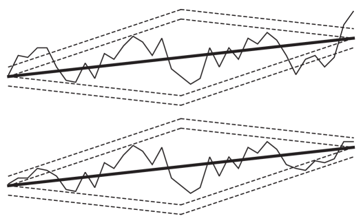
Figure 6.1: Shown here are $\phi_{u}$ (dark lines); $\phi_{u}\pm\epsilon nf(nx)$ and $\phi_{u}(x)\pm(\epsilon nf(nx)+\epsilon)$ (dotted lines); and $\phi$ before and after a random truncation (where $d=1$).

Now, we claim that $FE_{\Lambda_{n}}(\mu_{n}^{\prime\prime})\leq FE_{\Lambda_{n}}(\mu_{n})+o(|\Lambda_{n}|)$. To see this, note that by Lemma 2.1.3, we can compute each relative entropy in stages: to sample from $\mu_{n}$ or $\mu_{n}^{\prime\prime}$, we can first choose $A^{+}$, then choose the values of $\phi$ conditioned on $A^{+}$. The relative entropy is the relative entropy of the first random process (the choice of $A^{+}$) plus the expected relative entropy of the second; similarly, the relative entropy of the choice of $\phi$ (conditioned on $A^{+}$) can be written as the relative entropy of the choice of $\phi$ for $x\not\in A^{+}$ plus the expected relative entropy of the choice of $\phi(x)$ for $x\in A^{+}$. Since the latter step is the only one which is different in the two process, the difference in the two relative entropies depends only on the expected difference in the relative entropy of the last two choices. For a given choice of $A^{+}$ and $\phi$ (defined for $x\not\in A^{+}$), write

$$Z^{-1}\pi_{0}=1_{p_{n}(x)\leq\phi(x),x\in A^{+}}e^{H^{o}_{\Lambda_{n}}(\phi)}\prod_{x\in A^{+}}d\phi(x),$$

where $Z$ makes the above a probability a measure; let $\pi$ )(resp., $\pi^{\prime\prime}$) be the conditional distribution of $\mu_{n}$ (resp. $\mu_{n}^{\prime\prime}$) conditioned on $A^{+}$ and $\phi$ (for $x\not\in A^{+}$). Since, by Corollary 6.1.3, the expected size of $|A^{+}|$ is $o(|\Lambda_{n}|)$, it is enough for us to show that $\mathcal{H}(\pi^{\prime\prime},\pi_{0})\leq\mathcal{H}(\pi,\pi_{0})+c|A^{+}|$ for some constant $c$. Since $\mathcal{H}(\pi,\pi_{0})$ is positive, it is enough to show $\mathcal{H}(\pi^{\prime\prime},\pi_{0})\leq c|A^{+}|$. The reader may check this last fact, again, by writing the relative entropy as a sum of a sequence of expected conditional relative entropies, one for each $x\in A^{+}$. The key observation is that when one chooses $\phi(x)$—and $\phi(y)$ have already been chosen for some nonempty subset $S_{x}$ of the neighbors $y$ of $x$, and each $\phi(y)\leq\phi_{u}(y)+\epsilon nf(y/n)$, then the measure $e^{-\sum_{y\in S_{x}}V((\phi(y)-\phi(x))s(y))}1_{\phi(x)\leq\phi_{u}(x)+\epsilon nf(y/n)}d\phi(x)$ (where $s(y)$ is $1$ if $x$ precedes $y$ lexicographically, and $-1$ otherwise) obtains a bounded fraction of its mass in the interval $[\phi_{u}(x)+\epsilon nf(y/n),\phi_{u}(x)+\epsilon nf(y/n)+1]$, independently of the precise values of $\phi(y)$.

To sample $\phi$ from $\mu^{\prime}_{n}$, first sample $\phi$ from $\mu_{n}^{\prime\prime}$, then apply a “lower truncation” (analogous to the upper truncation described above, using $A^{-}$ instead of $A^{+}$) and condition on the output lying in $B_{n}$. Since, by the ergodic theorem, the probability of the latter event tends to one, we have $FE_{\Lambda_{n}}(\mu_{n}^{\prime})\leq FE_{\Lambda_{n}}(\mu_{n})+o(|\Lambda_{n}|)$, as desired.

6.1.2 $PBL(\mu)\leq SFE(\mu)$ for general $\mu$

Since $SFE$ is affine, it is enough to show that $PBL(\mu)$ is “strongly convex”—i.e., that when $\mu=\int\nu w_{\mu}(\nu)d\nu$, we have $PBL(\mu)\leq\int PBL(\nu)w_{\mu}(\nu)d\nu$.

First we will show that $PBL$ is convex. Suppose that $\mu_{1}$ and $\mu_{2}$ have slopes $u_{1}$ and $u_{2}$ respectively, $0<a<1$, $\mu=a\mu_{1}+(1-a)\mu_{2})$, and $u=au_{1}+(1-a)u_{2}$. It is enough to show that $PBL^{u}_{B}{\mu}$ is less than or equal to $PBL^{u_{1}}(\mu_{1})+PBL^{u_{2}}(\mu_{2})$ for each $B\ni\mu,B\in\mathcal{B}$. We may assume $B$ is a finite intersection of sets of the form $\{\pi:|\pi(F_{j})-\mu(F_{j})|\leq\epsilon\}$, where each $F_{j}:\Omega\rightarrow[0,1]$ is a cylinder function. For $i\in\{1,2\}$, take $B^{i}$ to be the intersection of the sets $\{\pi:|\pi(F_{j})-\mu_{i}(F_{j})|\leq\epsilon/2\}$. By the definition of $PBL$, it is now enough to show that $PBL^{u}_{B}{\mu}$ is less than or equal to $aPBL^{u_{1}}_{B^{1}}(\mu_{1})+(1-a)PBL^{u_{2}}_{B^{2}}(\mu_{2})$. And to prove this, it is enough to us to show that for any fixed $n$, letting $M$ get large, we have

$$-|\Lambda_{M}|^{-1}\log\left(\int 1_{A_{M}\cap B_{M}}e^{-H^{o}_{\Lambda}(\phi)}\prod_{x\in\Lambda_{n}\backslash\{x_{0}\}}d\phi(x)\right)\leq$$

$$-a|\Lambda_{n}|^{-1}\log\left(\int 1_{A_{n}\cap B^{1}_{n}}e^{-H^{o}_{\Lambda}(\phi)}\prod_{x\in\Lambda_{n}\backslash\{x_{0}\}}d\phi(x)\right)-$$

$$(1-a)|\Lambda_{n}|^{-1}\log\left(\int 1_{A_{n}\cap B^{2}_{n}}e^{-H^{o}_{\Lambda}(\phi)}\prod_{x\in\Lambda_{n}\backslash\{x_{0}\}}d\phi(x)\right)+o(1).$$

Next, roughly speaking, we would like to combine $\phi_{u_{1}}$ and $\phi_{u_{2}}$ to form a “washboard” function of slope $u$ whose gradient agrees with that of $\phi_{u_{1}}$ on an $a$ fraction of the points and that of $\phi_{u_{2}}$ on a $(1-a)$ fraction of points. (See Figure 6.2.)

Write $p_{1}=(1-a)$ and $p_{2}=a$. Fix some large integer $N$ and consider the layered sequence of surfaces $\phi^{j}_{u_{i}}(x)=\phi_{u_{i}}(x)+p_{i}Nj$ (for $j\in\mathbb{Z}$); let $\tilde{\phi}_{u_{i}}(x,\eta)$ give the index $j$ of the lowest layer which lies beneath the point $(x,\eta)$, i.e., the smallest $j$ for which $\phi^{j}_{u_{i}}(x)\leq\eta$.

Now, write $\psi(x)=\inf\{\eta|\tilde{\phi}_{u_{1}}(x,\eta)+\tilde{\phi}_{u_{2}}(x,\eta)\leq 0$. Now, fix $n$ and tile $\mathbb{Z}^{d}$ with a sequence $\Delta_{j}$ of cubes of side-length $n$. It is not hard to see, for fixed $n$, that $\psi$ has asymptotic slope given by $u$ and that the fraction of cubes on which the gradient of $\psi$ fails to agree with that of either $\phi_{1}$ or $\phi_{2}$ throughout the cube is $o(\frac{1}{N})$. Moreover, if $\epsilon$ is the minimum of the $\epsilon$ values in the definitions of $\phi_{u_{1}}$ and $\phi_{u_{2}}$, then the energy at any edge of $\phi$ will be less than or equal to $C$ whenever $\phi$ is sampled from the box measure of radius $\epsilon$ centered at $\psi$.

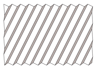
Figure 6.2: A “washboard” shaped surface $\psi$ when $d=2$. The shaded regions have slope $u_{1}$ and the unshaded regions have slope $u_{2}$.

Define $\nu_{n}$ to be the measure $1_{A_{n}\cap B_{n}}e^{H^{o}_{\Lambda_{n}}}\prod_{x\in\Lambda_{n}\backslash\{x_{0}\}}d\phi(x)$; define $\nu^{i}_{n}$ analogously using $B^{i}_{n}$ instead of $B$. We can restate our goal as follows: we need to prove that as $N$ and $M$ get large,

$$|\Lambda_{M}|^{-1}FE(\nu_{M})\leq a|\Lambda_{n}|^{-1}FE(\nu^{1}_{n})+(1-a)|\Lambda_{n}|^{-1}FE(\nu^{2}_{n})+o(1).$$

Since $\nu_{M}$ has minimal free energy among measures supported on $A_{M}\cap B_{M}$, it is enough to generate some measure $\nu^{\prime}_{M}$ supported on $A_{M}\cap B_{M}$ for which the analogous expression holds.

Now, we define a measure $\nu^{\prime}_{M}$ on $(\Omega,\mathcal{F}^{\tau}_{\Lambda})$ as follows. To sample from $\nu^{\prime}_{M}$, first choose $\phi$ from the radius-$\epsilon$ box measure centered at $\psi$ on $\Lambda$. Then, for all cubes $\Delta_{j}$ on which the gradient of $\psi$ is identically equal to that of either $\phi_{u_{1}}$ or $\phi_{u_{2}}$ (say $\phi_{u_{i}}$), we re-sample $\phi$ from $\nu^{i}_{n}$ (when $\Delta$ is translated to coincide with $\Lambda_{n}$ for the purposes of the definition). Letting $N$ and $M$ get large in such a way that $M/N\rightarrow\infty$, we see that

$$|\Lambda_{M}|^{-1}FE(\nu_{M})\leq a|\Lambda_{n}|^{-1}FE(\nu^{1}_{n})+(1-a)|\Lambda_{n}|^{-1}FE(\nu^{2}_{n})+o(1).$$

Moreover, if we modify $\nu^{\prime}_{M}$ by adding a truncation (as in the previous section) this modification will also change the normalized free energy by at most $o(1)$, and the result follows.

It remains to check that $PBL(\mu)$ is “strongly convex”—i.e., that when $\mu=\int\nu w_{\mu}(\nu)d\nu$, we have

$$PBL(\mu)\leq\int PBL(\nu)w_{\mu}(\nu)d\nu.$$

However, it is obvious from the definition of $PBL$ that it is lower semi-continuous in the topology of local convergence. So it is enough to observe that we can approximate $\mu$ in this topology by a sequence of slope-$u$ weighted averages of the form $\mu^{k}=\sum_{i=1}^{k}a_{i,k}\mu_{i,k}$ where $0\leq a_{i}\leq 1$, the $\mu_{i}$ are ergodic, the $\mu^{k}$ converge to $\mu$ in the topology of local convergence, and $\limsup SFE(\mu^{k})\leq SFE(\mu)$.

If one samples a sequence $\mu_{i}$ of ergodic components independently from $w_{\mu}$, then the law of large numbers implies that $\nu_{n}=\frac{1}{n}\sum_{i=1}^{n}\mu_{i}$ converges to $\mu$ in the topology of weak local convergence and that $SFE(\nu_{n})\rightarrow SFE(\mu)$ almost surely. The desired approximation is now easily obtained by altering the coefficients of the $\nu_{n}$ slightly (so that the slope is exactly $u$ instead of approximately $\nu$).

6.1.3 Empirical measure argument: $SFE(\mu)\leq FBL(\mu)$

Recall the definition

$$FBL_{B}(\mu)=\liminf_{n\rightarrow\infty}-|\Lambda_{n}|^{-1}\int 1_{B_{n}}e^{-H^{o}_{\Lambda}(\phi)\prod_{x\in\Lambda_{n}\backslash\{x_{0}\}}}d\phi(x).$$

We can normalize the measure $1_{B_{n}}e^{-H^{o}_{\Lambda}(\phi)\prod_{x\in\Lambda_{n}\backslash\{x_{0}\}}}d\phi(x)$ to produce a probability measure on the set of functions from $\Lambda_{n}\backslash\{x_{0}\}$ to $\mathbb{R}$. We can extend this to a probability measure $\nu^{n}_{B}$ on $\Omega$ in which the events $\phi(x_{0})=0$ and $\phi(x=\infty),x\not\in\Lambda_{n}$ have probability one. Let $\Lambda_{n}^{m}$ be the subset of $\Lambda_{n}$ containing vertices which are at least $m$ units in distance from the boundary of $\Lambda_{n}$. Now, let $m(n)$ be some function of $n$ for which $m(n)$ tends monotonically to $\infty$ in $n$ but $m(n)=o(n)$. Let $\mu^{n}_{B}=|\Lambda_{n}^{m(n)}\cap k\mathbb{Z}^{d}|^{-1}\sum_{y\in\Lambda_{n}^{m(n)}\cap k\mathbb{Z}^{d}}\theta_{y}\nu^{n}_{B}$.

Lemma 6.1.4

As $n$ tends to infinity along an increasing sequence for which

$$-|\Lambda_{n}|^{-1}\int 1_{B_{n}}e^{-H^{o}_{\Lambda}(\phi)\prod_{x\in\Lambda_{n}\backslash\{x_{0}\}}}d\phi(x)\rightarrow FBL_{B}(\mu),$$

at least one subsequential limit $\mu_{B}$ of the measures $\mu^{n}_{B}$ exists; any such limit satisfies

$$SFE(\mu_{B})\leq FBL_{B}(\mu).$$

Fix any integer $r>1$ and suppose that $\Delta_{1},\ldots\Delta_{j}$ are disjoint translations of $\Lambda_{r}$ contained in $\Lambda_{n}$. Then Lemma 2.3.1 implies that

$$FE_{\Lambda_{n}}(\nu^{n}_{B})\geq\sum_{i=1}^{j}FE_{\Delta_{i}}+c\left(|\Lambda_{n}\backslash\cup_{i=1}^{j}\Delta_{i}|+j\right),$$

where $c$ is a fixed constant—namely, the minimum possible value of $FE_{e}(\mu)$ where $e$ is a single edge. Now, if $n$ is large enough so that $m(n)>r$, then $\mu_{n}$, restricted to $\Lambda_{r}$, is a weighted average of the restrictions of $\nu_{n}$ to translations $\Delta_{1},\ldots,\Delta_{(n-m(n))^{d}}$ of $\Lambda_{r}$. We can divide $\{\Delta_{i}\}$ into $r^{d}=|\Lambda_{r}\cap k\mathbb{Z}^{d}|$ sub-collections according to the values of the components of their lexicographically minimal corners modulo $rk$; each such sub-collection consists of disjoint copies of $\Lambda_{r}$. Using convexity of free energy for the first step, we may conclude:

$$|\Lambda_{r}\cap k\mathbb{Z}^{d}|^{-1}FE_{\Lambda_{r}}(\mu^{n}_{B})\leq r^{-d}$$

$$\sum_{i=1}^{(n-m(n)^{d})}(n-m(n))^{-d}FE_{\Delta_{i}}\nu^{n}_{B}\leq$$

$$(1-o(n))|\Lambda_{n}\cap k\mathbb{Z}^{d}|^{-1}FE_{\Lambda_{n}}(\nu^{n}_{B})-o(n)+c(r^{-d})$$

This implies that

$$\limsup|\Lambda_{r}|^{-1}FE_{\Lambda_{r}}(\mu_{n})\leq\limsup|\Lambda_{n}|^{-1}FE_{\Lambda_{n}}(\nu^{n}_{B})=FBL_{B}(\mu).$$

By Lemma 2.1.5, this also implies that $\mu_{n}$ restricted to $\Lambda_{r}$ has a subsequential limit. By a diagonalization argument, we can can choose a subsequence for which such a limit exists for every $r$; and in this case, and this subsequence converges to a measure $\mu_{B}$ on $(\Omega,\mathcal{F}^{\tau})$, which is easily seen to be $\mathcal{L}$-invariant and satisfy $FE_{\Lambda_{r}}(\mu_{B})\leq FBL_{B}(\mu)-cr^{-d}$. Since this is true for any $r$, we have $SFE(\mu_{B})\leq FBL_{B}(\mu)$.   

Now, by Lemma 2.1.7, the set $M_{FBL(\mu)}=\{\nu:SFE(\nu)\leq FBL(\mu)\}$ is metrizable in the topology of weak local convergence. Hence, we can choose a sequence of sets $B^{m}\in\mathcal{B}$ in such a way that each is contained in the ball of radius $1/m$ about $\mu$ with respect to this metric. It is then clear that $\mu_{B^{m}}\rightarrow\mu$; hence, by Lemma 6.1.4 and Theorem 2.4.2,

$$SFE(\mu)\leq\liminf_{m\rightarrow\infty}SFE(\mu_{B^{m}})\leq\limsup_{m\rightarrow\infty}FBL_{B^{m}}(\mu)=FBL(\mu).$$

6.1.4 Alternate definition of $\sigma$

Theorem 6.1.1 also implies the following alternative definition of $\sigma$:

Corollary 6.1.5

If $\Phi$ is an SAP and $E=\mathbb{R}$ or $E=\mathbb{Z}$, then

$$\sigma(u)=\liminf_{n\rightarrow\infty}-|T_{n}|^{-1}\log Z_{T_{n}}\geq SFE(\mu),$$

where $Z_{T_{n}}$ are as defined in Section 4.2 and $\mu$ is the subsequential limit of the measures $\mu^{n}_{u}$ described in Lemma 4.2.6.

• Suppose $E=\mathbb{R}$. By tiling $T_{n}$ with large cubes and considering measures obtained by taking a box measure centered at $\phi_{u}$ outside of the cubes and then sampling the interiors according to a Gibbs measure, it is easy to see that for any $\mu$ with slope $u$,

  $$\liminf_{n\rightarrow\infty}-|T_{n}|^{-1}\log Z_{T_{n}}\leq PBL(\mu)=SFE(\mu).$$

  Hence,

  $$\sigma(u)\geq\liminf_{n\rightarrow\infty}-|T_{n}|^{-1}\log Z_{T_{n}}.$$

  For the other direction, it is enough to construct a measure $\mu$ with

  $$SFE(\mu)\leq\liminf_{n\rightarrow\infty}-|T_{n}|^{-1}\log Z_{T_{n}},$$

  and we can choose a subsequential limit $\mu$ of the torus measures which has this property. We will discuss the case $E=\mathbb{Z}$ in the next section.   

6.2 Limit equalities in other settings

6.2.1 Discrete systems

In this section, we describe the modifications to the proof of Theorem 6.1.1 necessary for the following discrete analog of the theorem.

Theorem 6.2.1

If $\Phi$ is an SAP, $E=\mathbb{Z}$, and $\mu\in\mathcal{P}_{\mathcal{L}}(\Omega,\mathcal{F}^{\tau})$, then

$$SFE(\mu)=FBL(\mu)=PBL(\mu).$$

If $E=\mathbb{Z}$, then the only relevant values of $V_{x,y}:\mathbb{R}\mapsto\mathbb{R}$ are the values assumed at integers. Thus, we lose no generality in making the convenient assumption that each $V_{x,y}$ is linearly interpolated between integer values — that is, $V_{x,y}$ is linear on $(j,j+1)$ for each $j\in\mathbb{Z}$, lower semi-continuous, and convex. (Thus, $V_{x,y}$ is continuous and finite on some closed interval $[i,j]$ with $i,j\in\mathbb{Z}\cup\{-\infty,\infty\}$, and infinite elsewhere.)

If $\phi:\mathbb{Z}^{d}\rightarrow R$ is any continuous configuration, then we can define a “randomly rounded” discrete configuration by $\phi^{\epsilon}=\lfloor\phi+\epsilon\rfloor$ where $\epsilon$ is chosen uniformly from $[0,1)$. A key observation is that the expected value of $V_{x,y}(\phi^{\epsilon}(y)-\phi^{\epsilon}(x))$ is equal to $V_{x,y}(\phi(y)-\phi(x))$.

Now, we take $\phi_{u}$ to be any real-valued function of slope $u$, with $\mathcal{L}$-periodic gradient, which has finite $\Phi$ energy. Now, we can define $FBL(\mu)$ and $PBL(\mu)$ precisely as in the continuous case except that when defining $PBL(\mu)$, we fix the boundary conditions by randomly rounding $\phi_{u}$. So $PBL^{B}_{\Lambda_{n}}(\mu)=FE_{\Lambda_{n}}(\mu_{n})$ where $\mu_{n}$ is define as follows: to sample from $\mu_{n}$, first choose $\phi$ on the boundary via a random rounding $\phi^{\epsilon}_{u}$ of $\phi_{u}$, where $\epsilon$ is chosen uniformly in $[0,1)$; then choose $\phi$ on the inside according to the Gibbs measure conditioned on the empirical measure lying in $B$ (i.e., on $\phi$ lying in $B_{n}$, as defined above). We define $FBL$ exactly as before.

Except for this change in setup, all of the arguments and definitions are essentially identical to the continuous cases. As before, it is obvious that $FBL(\mu)\leq PBL(\mu)$, and the argument that $SFE(\mu)\leq FBL(\mu)$ is the same as before. In the proof that $PBL(\mu)\leq SFE(\mu)$, however, there is a slightly difference in that we no longer need to define box measures, since singleton measures themselves have finite free energy, and the “random truncation” can be replaced by a non-random one. For the alternate definition of $\sigma$, since we cannot necessarily cause the slope of a configuration on the torus $T_{n}$ to be exactly $u$, we have to round $u$ to an integer vector multiple of $1/n$ (as described in Lemma 4.2.6). However, the remainder of the proof is the same as the continuous case.

6.2.2 Higher dimensions and PSAPs

Finally, in this section, we give the most general form of Theorem 6.1.1:

Theorem 6.2.2

If $\Phi$ is a perturbed SAP, $E=\mathbb{Z}^{m}$ or $E=\mathbb{R}^{m}$, and $\mu\in\mathcal{P}_{\mathcal{L}}(\Omega,\mathcal{F}^{\tau})$, then

$$SFE(\mu)=FBL(\mu)=PBL(\mu).$$

First, note that $\Phi$ is an SAP (which we can write $\Phi=\sum_{i=1}^{m}\Phi_{i}$, where each $\Phi_{i}$ is a one-dimensional SAP), then the definitions of $PBL$ and $FBL$ are the same as those given at the beginning of Section 6.1 except that $\phi_{u}=\prod_{i=1}^{m}\phi_{u}^{i}$, $A_{n}=\prod_{i=1}^{m}A^{i}_{n}$, and $B_{n}=\prod_{i=1}^{m}B^{i}_{n}$ where the $A_{i}^{n}$ and $B^{i}_{n}$ are subsets of functions from $\Lambda_{n}$ to $\mathbb{R}$, defined as they would be if we were in the one-dimensional setting using $\Phi_{i}$ and $u_{i}$ (the $d$-dimensional slope determined by the $i$th row of $u$) instead of $\Phi$. If $\Phi+\Psi$ is a perturbed SAP, where $\Phi$ strictly dominates $\Psi$, then we will also define $A_{n}$ and $B_{n}$ using $\Phi$.

• In both the $m>1$ and perturbed settings, the arguments for $SFE(\mu)\leq FBL(\mu)$ is exactly the same as before; in each setting, as in the simplest one-dimensional case, it is obvious from the definitions that $FBL(\mu)\leq PBL(\mu)$.

  In the un-perturbed case when $m>1$, the proof that $PBL(\mu)\leq SFE(\mu)$ for $\mu$ ergodic is the same as in the one-dimensional case except that we apply a separate randomized truncation in each of the $m$ coordinate directions. The generalization of this result to non-ergodic $\mu$ is exactly the same as the proof given for $E=\mathbb{R}$.

  In the perturbed case where the potential is defined to be $\Phi+\Psi$ (where $\Phi$ is simply attractive and strictly dominates $\Psi$, and $\Psi$ has range $k<\infty$), instead of defining $A_{n}$ to be the set for which the boundary values $\phi(x)-\phi(x_{0})$ (for $x\in\partial\Lambda_{n}$) are within $\epsilon$ of $\phi_{u}(x)-\phi_{u}(x_{0})$, we take $A_{n}$ to be the set in which $|(\phi(x)-\phi(x_{0}))-(\phi_{u}(x)-\phi_{u}(x_{0}))|<\epsilon$ for all $x\in\Lambda_{n}$ which are within $k$ units of distance from $\partial\Lambda_{n}$. Then we use the one-dimensional argument (just as before) to produce a random truncation in which the expected energy added each time we decide $\phi(x)$ for another $x\in A^{+}$ is finite; then we observe that since the expected combined $\Phi$ energy that occurs in edges within $k$ units of points in $A^{+}$ is $o(|\Lambda_{n}|)$, the expected combined $\Psi$ energy is $o(|\Lambda_{n}|)$ as well.   

6.3 Variational principle

We have already proved in Lemma 2.5.2 that if $\mu\in\mathcal{P}_{\mathcal{L}}(\Omega,\mathcal{F}^{\tau})$ has finite slope $u$ and $SFE(\mu)=\sigma(u)$, then $\mu$ must be a Gibbs measure. This, together with the converse, is called the variational principle.

Theorem 6.3.1

Let $\Phi$ be a perturbed ISAP (when $E=\mathbb{R}^{m}$ or $\mathbb{Z}^{m}$) or a perturbed LSAP (when $E=\mathbb{Z}^{m}$). Then if $\mu$ is an ergodic gradient measure of finite slope $u$, then $\mu$ is a Gibbs measure if and only if $SFE(\mu)=\sigma(u)$. If $\mu$ is a not-necessarily-ergodic gradient Gibbs measure with ergodic decomposition given by

$$\mu=\int_{\text{ex}\mathcal{P}_{\mathcal{L}}(\Omega,\mathcal{F}^{\tau})}w_{\mu}(\nu)d\nu,$$

then (letting $S(\nu)$ denote the slope of $\nu$) $\mu$ is a Gibbs measure if and only if

$$SFE(\mu)=w_{\mu}(\sigma(S*))$$

(using the abbreviation $w_{\mu}(\sigma(S*)):=\int_{\text{ex}\mathcal{P}_{\mathcal{L}}(\Omega,\mathcal{F}^{\tau})}w_{\mu}\sigma(S(\nu))d\nu$).

We will first observe here that the second statement follows from the first; we will then prove the first statement in case that $E=\mathbb{R}$ and $\Phi=\Phi_{V}$ is an ISAP, delaying the more general discussion until Section 6.4.

• The second statement in the lemma follows from the first, using Lemma 3.3.4 and the fact that slope is $e(\text{ex}\mathcal{P}_{\mathcal{L}}(\Omega,\mathcal{F}^{\tau}))$ measurable. For the first statement, by Lemma 2.5.2, we need only show that if $\mu$ is an ergodic Gibbs measure of slope $u$, then $SFE(\mu)\leq\sigma(\mu)$. By Lemma 6.1.1 (noting that in the definition of $PBL$ and any $\mu$ of slope $u$, the limit defining $PBL^{u}_{B}(\mu)$ only gets smaller if we replace $A_{n}\cap B_{n}$ with $A_{n}$—i.e., if we take $B=\Omega$), it is enough to show

  $$SFE(\mu)\leq\liminf_{n\rightarrow\infty}-|\Lambda_{n}|^{-1}\log\int_{A_{n}}e^{-H^{o}_{\Lambda_{n}}(\phi)}\prod_{x\in\Lambda_{n}\backslash\{x_{0}\}}d\phi(x).$$

  By Lemma 2.4.2, if we can construct a sequence $\mu_{n}$ of slope $u$ measures with

  $$\lim_{n\rightarrow\infty}SFE(\mu_{n})=\liminf_{n\rightarrow\infty}-|\Lambda_{n}|^{-1}\log\int_{A_{n}}e^{-H^{o}_{\Lambda_{n}}(\phi)}\prod_{x\in\Lambda_{n}\backslash\{x_{0}\}}d\phi(x),$$

  and $\mu_{n}$ converging weakly to $\mu$, then it will follow that $SFE(\mu)\leq\sigma(u)$.

  We define measures $\mu_{n}^{\epsilon}$ as follows: to sample from such a measure, first tile $\mathbb{Z}^{d}$ with cubes of size $\Lambda_{n}$; on each cube, we will independently choose a configuration belonging to $A_{n}$ in the following way. First, sample $\phi$ from $\mu$ and consider its restriction to $\Lambda_{n}$; we condition on the event that $\overline{H}^{o}_{\Lambda_{n}}(\phi)\leq C|\Lambda_{n}|$ where $C$ is twice the specific $\overline{V}$ energy of $\mu$ (a value which is finite by Lemma 4.1.8 and Lemma 2.3.8). The ergodic theorem implies the probability of this event tends to one as $n$ tends to $\infty$. Then, we let $\phi_{O}$ be the the outside interpolation function whose existence is guaranteed by Lemma 5.3.5 and we re-sample the values in $\Lambda_{n}\backslash\Lambda_{(1-\epsilon)n}$ according to the box measure (whose existence is guaranteed by Lemma 4.1.10) centered at $\phi_{O}$. (Throughout this argument, we tacitly assume that $(1-\epsilon)n$ is rounded down to the nearest integer.)

  Now, we would like to show that for any $\delta$, if $\epsilon$ is small enough, and $n$ large enough, then the specific free energy will be less $\delta+SFE(\mu)$. To see this, we will prove the result for measures $\nu_{n}^{\epsilon}$ whose specific free energies are clearly higher than those of the $\mu_{n}^{\epsilon}$. To sample from $\nu_{n}^{\epsilon}$, first sample form $\mu_{n}^{\epsilon}$, and then on each box, let $\phi_{I}$ be the interpolation between $\Lambda_{(1-\epsilon)n}$ and $\Lambda_{(1-\epsilon)^{2}n}$ guaranteed by Lemma 5.3.5; then re-sample using the values in $\Lambda_{(1-\epsilon)n}\backslash\Lambda_{(1-\epsilon)^{2}n}$ from the box measure whose existence is guaranteed by Lemma 4.1.10. This measure is equal to the Gibbs measure on $A_{(1-\epsilon)n}$ in the blocks forming a $(1-\epsilon)^{2}$ fraction of $\mathbb{Z}^{d}$, and outside, equal to a box measure with specific free energy bounded by a constant (again, by Lemma 4.1.10). Thus, for a sufficiently small $\epsilon$, we have that for sufficiently large $n$, $SFE(\nu^{\epsilon}_{n})\leq SFE(\mu)+\delta$. It is now trivial to check that $\mu$ is a limit point of the measures $\mu^{\epsilon}_{n}$.   

6.4 Variational principle in other settings

6.4.1 Discrete models

To prove Theorem 6.3.1 in the setting $E=\mathbb{Z}$, we take $\overline{V}=V$ (as before, assuming $V$ is linear between integers and lower semi-continuous) and construct continuous interpolations exactly as in the $E=\mathbb{R}$ setting. Our definition of $\mu_{n}^{\epsilon}$ and $\nu_{n}^{\epsilon}$ is essentially the same as in the previous case. We tile by $\Lambda_{n}$ blocks just as before, and choose the interpolations just as before; the only difference is that instead of using a box measure, we use a random rounding: i.e., we add a variable uniformly distributed in $[0,1]$ to the entire choice of $\phi$ and then round down (in the set $R$ consisting of points outside of the $(1-\epsilon)^{2}$ boxes), after which we sample the remainder of $\phi$ inside each of the boxes according to the appropriate Gibbs measure (with boundary conditions given by the values of $\phi$ in $R$).

6.4.2 Lipschitz simply attractive potentials

In the Lipschitz models—when $\Phi$ is not necessarily an ISAP, and we may not have a good definition of $\overline{V}$—we define $\mu_{n}^{\epsilon}$ and $\nu_{n}^{\epsilon}$ slightly differently: in this case, we use a truncation of the kind used in the proof that $PBL(\mu)\leq SFE(\mu)$ in Section 6.1.1. Because $\mu$ is Lipschitz, Lemma 6.1.2 actually implies that as $n$ tends to infinity, the probability that $\phi$ sampled from $\mu$ differs from the plane of slope $S(\mu)$ (with appropriate additive constant) by more than $\epsilon n$ in the supremum norm tends to zero in $n$. Thus, as $n$ gets large, the probability tends to one that truncations of the type in used in Lemma 6.1.1 will not affect the value of $\phi$ anywhere inside the box $\Lambda_{(1-\epsilon)n}$. These truncations play the role of the interpolations used in the non-Lipschitz setting. It is not hard to define an “inside truncation” in a similar fashion, to play the role of the inside interpolations.

6.4.3 Higher dimensions and perturbed ISAPs and LSAPs

The change to higher dimensions (without perturbations) is essentially trivial; we simply define the interpolations separately on each coordinate as before. The change to perturbed potentials $\Phi+\Psi$ is also essentially trivial; we simply observe that if the expected $\Phi$ energy in $\Lambda_{n}\backslash\Lambda_{(1-\epsilon)^{2}n}$ is $o(|\Lambda_{n}|)$, the expected $\Psi$ energy is $o(|\Lambda_{n}|)$ as well.

Chapter 7 LDP for empirical measure profiles

7.1 Empirical measure profiles and statement of LDP

Let $D$ be a bounded domain, and the sequence $D_{n}$ a good approximation of $D$. The aim of this chapter is to prove a large deviations principle (of speed $n^{d}$) for the behavior of a random gradient configuration $\phi_{n}$ on $D_{n}$. Instead of merely considering the gradient empirical measures—as in the previous section—we will consider profiles, which also contain information about how the occurrence of various gradient events are distributed throughout $D$. We will also investigate behavior of the normalized functions $\frac{1}{n}\phi_{n}(nx)$ (interpolated to functions on $D$) and examine their large deviations behavior with respect to topologies induced by $L^{p}$ and Orlicz $L^{A}$ metrics. We can define an empirical profile measure $R_{\phi_{n},n}\in\mathcal{P}(D\times\Omega)$ by

$$R_{\phi_{n},n}=\int_{D}\delta_{x,\mathcal{\theta}_{\lfloor nx\rfloor}\phi_{n}}dx.$$

Informally, to sample a point $(x,a)$ we choose $x$ uniformly from $D$, and then take $a=\theta_{\lfloor nx\rfloor}\phi_{n}$. (As in the previous chapter, it is convenient to write $\phi_{n}(x)=\infty$ for $x\not\in D_{n}$.) Also, using $\phi_{n}$, we will define a function $\tilde{\phi}_{n}$ by interpolating the function $\frac{1}{n}\phi_{n}(nx)$ to a continuous, piecewise linear (on simplices) function on the simplex domain corresponding to $D_{n}$; each such $\tilde{\phi}_{n}$ is a member of the space $L^{\overline{V}^{*}}_{0}(D)$ constructed in Section 5.2.2 for Corollary 5.2.4, where we take $\overline{V}^{*}$ to be any function increasing essentially more slowly that $\overline{V}_{d}$, where $\overline{V}$ is defined as in Section 4.1, and $\overline{V}_{d}$ is the Sobolev conjugate as defined in Section 5.1.4.

Write $\mu_{n}=Z_{n}^{-1}e^{-H^{o}_{D_{n}}(\phi)}\prod_{x\in D_{n}\backslash\{x_{0}\}}d\phi(x)$ where the $Z_{n}$ are normalizing constants chosen to make $\mu_{n}$ probability measures. Let $\rho_{n}$ be the measure on $X=\mathcal{P}(D\times\Omega)\times L^{\overline{V}^{*}}_{0}(D)$ induced by $\mu_{n}$ and the map $\phi_{n}\mapsto(R_{\phi_{n},n},\tilde{\phi}_{n})$. We say a measure $\mu\in\mathcal{P}(D\times\Omega)$ is $\mathcal{L}$-invariant if $\mu(\cdot,\Omega)$ is a Lebesgue measure on $D$ and for any $D^{\prime}\subset D$ of positive Lebesgue measure, $\mu(D^{\prime},\cdot)$ is an $\mathcal{L}$-invariant measure on $\Omega$. Given any subset $D^{\prime}$ of $D$ with positive Lebesgue measure, we can write $S(\mu(D^{\prime},\cdot))$ for the slope of the measure $\mu(D^{\prime},\cdot)/\mu(D^{\prime}\times\Omega)$ (we have normalized to make this a probability measure) times $\mu(D^{\prime}\times\Omega)$; the map $D^{\prime}\mapsto S(\mu(D^{\prime},\cdot))$ is a signed/vector-valued measure on $D$. Let $\mathcal{X}$ be the topology on $\mathcal{P}(D\times\Omega)\times L^{\overline{V}^{*}}(D)$ which is the product of (on the first coordinate) the smallest topology in which $\mu\rightarrow\mu(D^{\prime}\times f)$ is measurable for all rectangular subsets $D^{\prime}$ of $D$ and bounded cylinder functions $f$ and (on the second coordinate) the $L^{\overline{V}^{*}}_{0}(D)$ topology. We say an ISAP $\Phi=\Phi_{V}$ is super-linear if $\lim_{\eta\rightarrow\infty}V(\eta)/\eta=\infty$; although many of our bounds still hold for ISAPs which are not super-linear, the full LDP, which we prove below, is false as stated when $V$ is not super-linear.

Theorem 7.1.1

If $\Phi$ is a super-linear ISAP. The measures $\rho_{n}$ satisfy a large deviations principle with speed $n^{d}$ and rate function

$$I(\mu,f)=\begin{cases}SFE(\mu(D,\cdot))-P(\Phi)&\text{$\mu$ is $\mathcal{L}$-invariant and $S(\mu(x,\cdot))=\nabla f(x)$}\\ &\text{\em as a distribution}\\ \infty&\text{otherwise}\\ \end{cases}$$

on the space $\mathcal{P}(D\times\Omega)\times L^{\overline{V}^{*}}(D)$ in the topology $\mathcal{X}$ described above.

In the case that $\Phi$ is an SAP and $E=\mathbb{R}$, the uniqueness of the minimizer of the rate function $I$ described above is an immediate consequence of the uniqueness of the gradient Gibbs measure of a given slope (Theorem 8.6.3) and the strict convexity of $\sigma$ (Theorem 8.6.2—which in particular implies that $\sigma$ has a unique minimum). This will also imply uniqueness of the rate function in the presence of boundary conditions (see Section 7.3.2).

7.2 Proof of LDP

Recall that, in general, a sequence of measures $\rho_{n}$ on a topological space $(X,\mathcal{X})$ is said to satisfy a large deviations principle with rate function $I$ and speed $n^{d}$ if $I:X\rightarrow[0,\infty]$ is lower-semicontinuous and for all sets $B\in\mathcal{X}$,

$$-\inf_{x\in B^{o}}I(x)\leq\liminf_{n\rightarrow\infty}n^{-d}\log\rho_{n}(B)\leq\limsup_{n\rightarrow\infty}n^{-d}\log\rho_{n}(B)\leq-\inf_{x\in\overline{B}}I(x).$$

Let $\mathcal{A}$ be any basis of $\mathcal{X}$. It is not hard to check (and is proved in [22], Theorem 4.1.11 and Lemma 1.2.18) that the large deviations principle is a consequence of the following three statements:

1. Lower bound on probabilities:

   $$\inf_{S\in\mathcal{A};x\in S}\limsup\frac{1}{n^{d}}\text{log}\rho_{n}(S)\geq-I(x).$$

2. Upper bound on probabilities:

   $$\inf_{S\in\mathcal{A};x\in S}\liminf\frac{1}{n^{d}}\text{log}\rho_{n}(S)\leq-I(x).$$

3. Exponential tightness: For every $\alpha<\infty$, there exists a compact set $K_{\alpha}\subset X$ for which $\limsup_{n\rightarrow\infty}n^{-d}\log\rho_{n}(X\backslash K_{\alpha})<-\alpha$.

The above conditions also imply that all the level sets $M_{\alpha}=\{x:I(x)\leq\alpha\}$ are compact (by Lemma 1.2.18 of [22]). When the first and second statement hold, we say that the $\rho_{n}$ satisfy a weak large deviations principle with rate function $I$. When the third statement holds, we say that the $\rho_{n}$ are exponentially tight. In the following subsections, we will prove Theorem 7.1.1 by checking each of these statements in turn. We will do this first for the simplest case—when $\Phi$ is an ISAP and $E=\mathbb{R}$—and address generalizations in Section 7.3.

7.2.1 Lower bounds on probabilities

The lower bound follows almost immediately from Lemma 5.4.3 and Lemma 5.4.4 and Theorem 6.1.1 —in particular, the fact that $SFE(\mu)=PBL(\mu)$.

Suppose we are given $I(f,\mu)<\infty$. This implies that $f\in L^{1,A}(D)$, and hence, by Lemma 5.4.3, for all $n$ sufficiently large, there exists a function $F_{\epsilon}\in L^{1,A}(D)$ that is equal to a piecewise linear approximator $F_{n}$ (as defined prior to Lemma 5.4.3) on a closed subset $D^{\prime}$ of $D$, where the volume of $D\backslash D^{\prime}$ is less than $\epsilon$ and $\int_{D-D^{\prime}}A(\nabla F_{\epsilon})\leq\epsilon$.

Now, a basis set $S\subset A$ centered at $f,\mu$ can be written as the set of pairs $(g,\nu)$ for which $\delta(f,g)<\gamma$ (for some $\gamma>0$, where $\delta$ is the distance function described in Section 5.2.2—roughly, $\delta(f,g)=||f-g||_{\overline{V}^{*}}$) and $|\mu(1_{D_{i}}H_{i})-\nu(1_{D_{i}}H_{i})|<\gamma$ for each of a finite set of cylinder functions $H_{i}$ (each bounded between $0$ and $1$) on $\Omega$ and rectangular subsets $D_{i}$ of $D$.

Assume without loss of generality (rescaling if necessary) that the volume of $D$ is less than one.

Now, given any $F_{\epsilon}$, and a large $n$, we define a measure $\mu_{\epsilon,n}$ on configurations on $D_{n}$ as follows: to sample $\phi$ from $\mu_{\epsilon,n}$, first compute the approximation $F_{\epsilon}^{n}:D_{n}\rightarrow\mathbb{R}$ of $F_{\epsilon}$ guaranteed by Lemma 5.4.4 (with $A=\overline{V}$) and fix $\phi(x_{0})=F_{\epsilon}^{n}(x_{0})$ for some reference vertex $v_{0}$. Then sample $\phi(x)$ from the box measure centered at $\mu_{\epsilon,n}$ (the one whose existence is given by Lemma 4.1.7) for all values of $x\in D_{n}\backslash\{x_{0}\}$ for which $x$ does not lie on the interior of one of the linear regions of $F_{\epsilon}$. The free energy of this process is, by Lemma 4.1.7 and Lemma 5.4.4 and the assumed bound on $\int_{D-D^{\prime}}A(\nabla F_{\epsilon})$, at most a constant times $\epsilon n^{d}$.

Then, inside each large box $\Delta_{n}$ of $D_{n}$—assume it has size $\Lambda_{k}$—approximating a box $\Delta$ on which $F_{\epsilon}$ is linear, we sample $\phi$ from (appropriately translated) the Gibbs measure on $A_{n}\cap G_{n}$ where $G$ is the set of measures $\nu$ for which $|\nu(H_{i})-\frac{\mu(H_{i}1_{D_{i}})}{|D_{i}|}|<\gamma/2$ for each $i$. See Figure 7.1.

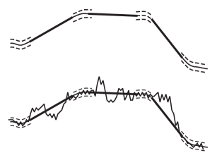
Figure 7.1: Above, a mostly linear function $F_{\epsilon}$, with dotted lines among the non-linear parts describing the bounds of a corresponding box measure), in the trivial case $d=1$. Below, an instance of $\phi$ sampled from $\mu_{n,\epsilon}$: in non-linear parts, $\phi$ is chosen from a box measure; in the linear parts, $\phi$ is chosen with empirical measure constraints.

If $\epsilon<\gamma/2$ and $n$ is sufficiently large, then it is not hard to see that $\mu_{\epsilon,n}$ is supported inside the set $S$. Since the free energy from the box measure choice in the non-linear sections of $\mu_{\epsilon,n}$ is $O(\epsilon n^{d})$, and the free energy from the remaining choice is at most $SFE(\mu(\overline{\Delta}\times\cdot)/\mu(\overline{\Delta}\times\Omega)$ times $n^{d}|\overline{\Delta}|$, where $\overline{\Delta}$ is the union of the square regions of $\mathbb{R}^{d}$ on which $F_{\epsilon}$ is linear. If follows from Theorem 6.1.1—since $SFE(\mu)=PBL(\mu)$—that $\limsup_{n\rightarrow\infty}\frac{1}{n^{d}}FE(\nu_{\epsilon,n})\leq I(f,\mu)+o(\epsilon)$, which implies the desired lower bound on probabilities.

7.2.2 Upper bounds on probabilities when $I(\mu,f)<\infty$

The upper bound follows almost immediately from Lemma 6.1.1—in particular, the fact that $SFE(\mu)=FBL(\mu)$. Since $I(\mu,f)<\infty$, $\mu$ is an $\mathcal{L}$-invariant gradient measure. Now, we may partition $D$ into disjoint cubes $K_{1},\ldots,K_{k}$ of equal size that cover at least a $1-\epsilon$ fraction of the Lebesgue volume of $D$, and let $K=\cup_{i=1}^{k}K_{i}$. In particular, for any basis set $S$, for a fine enough partition, we will have $\mu(K,\cdot)/\mu(K,\Omega)$; the $\liminf$ of the average specific free energy within $K$—as we choose $S$ small enough so that $\nu(K,\cdot)$ lies in a sufficiently small neighborhood of $\mu(K,\cdot)$—is at least $SFE(\mu(K,\cdot))$. As $\epsilon$ tends to zero, $\mu(K,\cdot)$ converges to $\mu(D,\cdot)$ in the topology of local convergence. The average specific free energy outside of $K$ is at least $\alpha$ (as defined in Corollary 2.3.2). This gives the desired bound.

7.2.3 Upper bounds on probabilities when $I(\mu,f)=\infty$

If $\mu$ is $\mathcal{L}$-invariant and $S(\mu(x,\cdot))=\nabla f(x)$ as a distribution and nonetheless $I(\mu)=\infty$ (because $SFE(\mu(D,\cdot)=\infty)$), then the argument is the same as in the previous section. We have now to show the upper bound on probabilities when either $S(\mu(x,\cdot))\not=\nabla f(x)$ as a distribution or $\mu$ is not $\mathcal{L}$-invariant.

First, if $\mu$ is not $\mathcal{L}$-invariant, then there is an event $H$ and a rectangle $D^{\prime}$ for which $\mu(D^{\prime}\times H)>\mu(D\times\theta_{x}H)+\delta$ for some $\delta>0$. We choose a neighborhood $S$ to be such that for each $(g,\nu)$ in this neighborhood, $\nu(D^{\prime}\times H)>\nu(D\times\theta_{x}H)+\delta/2$. Now, it is not hard to see that the probability of belonging to this neighborhood becomes zero when $n$ is large enough.

Second, suppose that there exists a rectangle $D^{\prime}$ for which $S(\mu(x,D^{\prime}))$ is not equal to the mean value of $\nabla f(x)$ on $D^{\prime}$. Suppose these two values disagree in the $i$th component direction—and suppose that $D^{\prime}$ has length $L$ in the $i$th direction and normal cross-sectional area given by $\alpha$. Then, integrating in the $i$th direction, this implies that the difference $\delta$ of the mean value of $f$ on opposite sides of $D^{\prime}$, divided by $L$, is different from $\mu(D^{\prime},\phi(e_{i})-\phi(0))$—different by, say, $\gamma>0$. Now, let

$$H_{C}(\phi)=\begin{cases}\phi(e_{i})-\phi(0)&|\phi(e_{i})-\phi(0)|\leq C\\ -C&\phi(e_{i})-\phi(0)<-C\\ C&\phi(e_{i})-\phi(0)>C\\ \end{cases}$$

By letting $C$ get large and choosing a neighborhood that ensures that the average value of $H_{C}$ on $D^{\prime}$ tends to the $S(\mu(x,D^{\prime}))$; by continuity of the average cross-sectional area, in $f$, if we take $S$ also to include a sufficiently tight restriction on $g$, then we can force the sum of $\phi(x+e_{i})-\phi(x)$ over an arbitrarily small fraction of the points $x$ to grow in $n$ like $\gamma n^{d}$. Since $V$ is super-linear, taking this fraction arbitrarily small implies, as desired, that

$$\inf_{S\in\mathcal{A};x\in S}\liminf\frac{1}{n^{d}}\text{log}\rho_{n}(S)\leq-\infty.$$

7.2.4 Exponential tightness

We define the set $K_{C}\subset\mathcal{P}(D\times\Omega)\times L^{\overline{V}^{*}}_{0}(D)$ to be the set of of profile/interpolation pairs corresponding to functions from $D_{n}$ to $\mathbb{R}$ with average $\overline{V}$ energy per edge equal to or less than $C$. Exponential tightness will follow once we show that

1. For each $C$, the set $K_{C}$ is pre-compact in $(X,\mathcal{X})$.

2. For any $\alpha>0$, if we choose $C$ large enough, we will have

   $$\liminf_{n\rightarrow\infty}n^{-d}\log\mu_{n}(K_{C}^{c})\leq-\alpha.$$

For the first statement, it is enough to show that the projection of $K_{C}$ onto each of its two components—in $\mathcal{P}(D\times\Omega)$ and in $L^{\overline{V}^{*}}_{0}(D)$—is pre-compact in the corresponding topology. The first is a simple exercise; the second follows from Lemma 5.2.4.

For the second statement, by Lemma 4.1.7, it is enough to prove an analogous statement using $V$ instead of $\overline{V}$. Suppose it were the case that for some $\alpha$,

$$\liminf\log\mu_{n}(1_{n^{-d}|H^{o}(\phi)|\geq C})\geq-\alpha$$

for every $C$. Then this would imply that if we replaced $\Phi$ with $(1-\epsilon)\Phi$, for any small $\epsilon>0$, then we would have

$$\liminf n^{-d}\log\int e^{-H^{o}(\phi)}\prod_{x\in D_{n}\backslash\{x_{0}\}}=\infty,$$

i.e., the log partition function growing super-exponentially in $n$. This is a contradiction to Corollary 2.3.2.

7.3 LDP in other settings

In this section, we briefly describe some variants Theorem 7.1.1 (to $E=\mathbb{Z}$ or $m>1$ or $\Phi$ not an ISAP) and describe the modifications to the proof required for these settings. However, we will not reproduce in detail the proof of Theorem 7.1.1 in each of these settings, as this would consume a good deal of space and the modifications are all straightforward.

7.3.1 Discrete models and Lipschitz models

All of the arguments in this chapter carry through to higher dimensional spin spaces, perturbed systems, and discrete models (using similar rounding arguments to those described in the previous chapter) with little or no modification. However, some additional care is required in the case that $E=\mathbb{Z}$ but $\Phi$ is Lipschitz, so that $V$ fails to be everywhere finite. In this case, $\sigma$ does not approach infinity near the boundary of the space of allowable slopes, so it is possible that the rate function $I(f,\mu)$ will be non-infinite even if $\nabla f_{\mu}(x)$ lies on this boundary for $x$ in a subset of $D$ with positive measure. If this is the case, we say that $f$ is a taut height function. Since the variational principle and the uniqueness of the gradient phase of slope $u$ (as shown in Chapter 8) may not apply when $u$ is one of these boundary slopes, we cannot expect the minimizer of the rate function to be unique in this case. However, the large deviations principle does go through. A simple analytical argument shows that we can always approximate a taut $(f,\mu)$ by a sequence of pairs $(f_{i},\mu_{i})$ for which the $f_{i}$ are not taut; this enables us to deduce the necessary lower bound, and the upper bounds and exponential tightness arguments are the same as before.

7.3.2 LDP with boundary conditions

In the continuous setting, we sometimes wish to limit our attention to functions $f$ that extend to the closure of $D$ and satisfy $f=f_{0}$ on $\partial D$, where $f_{0}:\partial D\rightarrow\mathbb{R}^{m}$ is a continuous boundary condition. Of course, elements of $L^{\overline{V}^{*}}(D)$ are not continuous for general $\overline{V}^{*}$, and in particular need not be continuous at the boundary of $D$. But we will say that a function $f$ on $D$ has $f_{0}$ as its boundary if $f$ is a limit in $L^{\overline{V}^{*}}(D)$ of functions in $L^{\overline{V}^{*}}(D)$, each of which agrees with $f_{0}$ outside of a compact subset of $\partial D$.

We would like to impose similar conditions on the discrete models. However, since none of the elements of the boundaries of the $D_{n}$ actually lies on the boundary of $\partial D$, we cannot simply require that $\phi(x)=f_{0}(x)$ for $x\in\partial D_{n}$. In fact, there are many ways to specify discrete boundary conditions; we will choose the one that is most convenient for us.

Assume that $f_{0}$ extends continuously to a function in $L^{1,A}(D)$; then we define as in the previous section the functions $f^{n}_{0}$, approximating $f_{0}$ on $D_{n}$, as in Lemma 5.4.4, and box measures $\nu_{n,\epsilon}$ centered at these functions. Now, take $\mu_{n}$ to be the sequence of measures $\mu_{n}=Z_{n}^{-1}e^{-H^{o}_{D_{n}}(\phi)}\prod_{x\in D_{n}\backslash\{x_{0}\}}1_{\chi_{n}}d\phi(x)$ where the $Z_{n}$ are normalizing constants chosen to make $\mu_{n}$ probability measures and each $\chi_{n}$ is the set of $\phi$ for which $|\phi(x)-f^{n}_{0}(x)|\leq\epsilon$ for each $x\in\partial D_{n}$. These induce measures $\rho_{n}$, defined as above.

Theorem 7.3.1

If $\Phi$ is a super-linear ISAP. The measures $\rho_{n}$ satisfy a large deviations principle with speed $n^{d}$ and rate function (up to an additive constant) given by

$$I(\mu,f)=\begin{cases}SFE(\mu(D,\cdot))-P(\Phi)&\text{$\mu$ is $\mathcal{L}$-invariant and $S(\mu(x,\cdot))=\nabla f(x)$}\\ &\text{ as a distribution and $f$ has $f_{0}$ as}\\ &\text{ its boundary}\\ \infty&\text{otherwise}\\ \end{cases}$$

on the space $\mathcal{P}(D\times\Omega)\times L^{\overline{V}^{*}}(D)$ in the topology $\mathcal{X}$ described above.

• We assume $m=1$ (the extension to $m>1$ being straightforward). Exponential tightness and the upper bounds on probabilities in the case that $f$ has $f_{0}$ as its boundary are the same as in the no-boundary case. If $f$ agrees with $f_{0}$ outside of a compact subset of $f$, then lower bound argument is also exactly the same as before (noting that the approximation of $f$ defined in Lemma 5.4.3 agrees with $f$—and hence $f_{0}$—on the boundary of $D_{n}$ for all large enough $n$); since, by definition, any $f$ that has $f_{0}$ as its boundary is a limit in $L^{\overline{V}^{*}}(D)$ of functions with this property, this gives the lower bound in general.

  It remains only to check the upper bound on probabilities in the case that $f$ does not have $f_{0}$ as its boundary (and hence $I(\mu,f)=\infty$). We know by compactness that the probability that the probability that $\phi$ fails to have a subsequential limit in $L^{\overline{V}^{*}}(D)$ tends to zero super-exponentially. However, in light of the discrete boundary conditions, it is not hard to see that any subsequential limit in $L^{\overline{V}^{*}}(D)$ of $\phi$ chosen from $\rho_{n}$ must have $f_{0}$ as its boundary.   

The generalization to LSAPs with $E=\mathbb{Z}$ is straightforward when $f_{0}$ is not taut, since in this case, any $f$ extending $f_{0}$ can be approximated by functions which are not taut. However, if $f_{0}$ is taut—for example, if it is a plane of slope $u$—then the empirical measure large deviations principle need not hold. If there are distinct ergodic Gibbs measures $\mu_{1}$ and $\mu_{2}$ of slope $u$ that have different specific free entropies, and $\phi_{1}$ and $\phi_{2}$ are samples from $\mu_{1}$ and $\mu_{2}$, then the large deviations behavior of the sequence of Gibbs measures with boundary conditions given by $\phi_{1}$ outside of $\Lambda_{n}$ will be different from the one with boundary conditions given by $\phi_{2}$ outside of $\Lambda_{n}$.

7.3.3 Gravity and other external fields

Let $h:X\rightarrow\mathbb{R}$ be any continuous function on $X$; we would now like to replace the measure $\rho_{n}$ with $\pi_{n}=e^{-h}\rho_{n}$ (times the normalizing constant that makes $\pi_{n}$ is a probability measure). These new measures $\pi_{n}$ clearly satisfy upper and lower bounds on probabilities described above when $I(x)$ is replaced by $I_{0}(x)=I(x)+h(x)$. When $m=1$, typical example of a continuous function $h$ might be (in the presence of boundary conditions) $h(f,\mu)=\int_{D}f(\eta)d\eta$— this corresponds to weighting a configuration with additional energy proportional to the “gravitational potential” energy of the surface (causing typical surfaces to sag lower in the interior of $D$). Another example of such an $h$ might be $h(f,\mu)=\mu(H)$ for some function $H:\Omega\rightarrow\{0,1\}$; this corresponds to weighting by the number of times a particular local configuration appears.

We would like to argue that for some constant $C$, the $\pi_{n}$ satisfy a large deviations principle with rate function $I(x)+h(x)+C$. But this follows immediately from Varadahn’s Integral Lemma (Theorem 4.3.1 of [22]) provided that a certain tightness conditions holds. Namely, we require

$$\lim_{M\rightarrow\infty}\limsup n^{d}\log E\left(e^{n^{d}h(x)}1_{h(x)\geq M}\right)=-\infty.$$

This holds for the gravitational potential described above (when $\sigma$ is super-linear) and many other kinds of external fields.

Chapter 8 Cluster swapping

Cluster swapping is a simple geometric operation that we will use to prove strict convexity of the surface tension function $\sigma$ and to classify $\mathcal{L}$-ergodic gradient Gibbs measures and their extremal decompositions (which may be non-trivial if $E=\mathbb{Z}$) whenever $\Phi$ is an $\mathcal{L}$-invariant simply attractive potential. Throughout this chapter and Chapter 9, we will assume that $m=1$, so that either $E=\mathbb{Z}$ or $E=\mathbb{R}$, and that $\Phi$ is an $\mathcal{L}$-invariant SAP.

The prerequisites for this chapter are Chapters 2, 3, and 4. The only results from Chapters 5, 6, and 7 that we will even mention in either this chapter or Chapter 9 are Corollary 6.1.5 (which gives the alternate definition of $\sigma$ using limits of log partition functions on tori) and the second half of the variational principle, Theorem 6.3.1; and the latter we mention only in the following remark.

Recall that the variational principle has two parts: the first, which we will use frequently, is Theorem 2.5.2, which states that whenever $SFE(\mu)=\sigma(S(\mu))$, the measure $\mu$ is a gradient Gibbs measure. This result holds for all simply attractive potentials. Recall also that a minimal $\mathcal{L}$-ergodic gradient phase of slope $u$ is defined to be a slope-$u$ $\mathcal{L}$-ergodic gradient Gibbs measure $\mu$ on $(\Omega,\mathcal{F}^{\tau})$ with minimal specific free energy; i.e., $SFE(\mu)=\sigma(u)$. In this chapter, we will classify the minimal $\mathcal{L}$-ergodic gradient phases of slope $u$ for any $u\in U_{\Phi}$.

The second half of the variational principle, Theorem 6.3.1, states that every $\mathcal{L}$-ergodic gradient phase $\mu$ of slope $u\in U_{\Phi}$ is in fact a minimal $\mathcal{L}$-ergodic gradient phase. We have proved the second half only for perturbed isotropic and (discrete) Lipschitz simply attractive potentials—it is not known whether Theorem 6.3.1 can be extended to all simply attractive potentials. In the cases where Theorem 6.3.1 is true, our classification of the minimal $\mathcal{L}$-ergodic gradient phases of slope $u$ may be interpreted as a classification of all $\mathcal{L}$-ergodic gradient phases of slope $u$.

8.1 Introduction to cluster swapping

8.1.1 Review: Fortuin-Kasteleyn; Swendsen-Wang;
Edwards-Sokal updates

Before describing cluster swapping, we review some facts about the related Swendsen-Wang algorithm, introduced in 1987 [84] and generalized to the form we present below by Edwards and Sokal in 1989 [30]. For this subsection only, we let $(E,\mathcal{E})$ be a finite set endowed with counting measure $\lambda$ (for example, $E$ could be $\{-1,1\}$, as in the Ising model), $\Lambda$ any finite graph with a subset $\partial\Lambda$ of its vertices designated as boundary vertices, and $\Phi=\{\Phi_{\Lambda}\}$ any Gibbs potential on functions $\xi:\Lambda\rightarrow E$. The crucial idea is the introduction of an independent random auxiliary function called the residual energy.

Let $(\xi,r)$ be a random pair in which $\xi:\Lambda\rightarrow E$ is sampled from the Gibbs measure $e^{-H^{\Phi}_{\Lambda}}\prod_{x\in\Lambda\backslash\partial\Lambda}d\xi(x)$ (times a normalizing constant), with boundary values $\xi=\xi_{0}$ fixed on $\partial\Lambda$, and $r$ is an independent function from the subsets of $\Lambda$ to $[0,\infty)$ where the values $r(\Delta)$ are all independent exponentials with parameter $1$, i.e., distributed according to the measure $e^{-x}dx$ on $[0,\infty)$. We refer to the quantity $r(\Delta)$ as the residual energy in $\Delta$, $\Phi_{\Delta}(\xi)$ as the potential energy in $\Delta$, and $t(\Delta):=r(\Delta)+\Phi_{\Delta}(\xi)$ as the total energy in $\Delta$. Note that the probability density of the pair $(\xi,r)$ with respect to the natural underlying measure (i.e., $\lambda^{|\Lambda\backslash\partial\Lambda|}$ times the product—over all $\Delta\subset\Lambda$—of Lebesgue measure on $[0,\infty)$) is proportional to $e^{-|t|}$ where $|t|=\sum_{\Delta\subset\Lambda}t(\Delta)$.

A general version of the random Swendsen-Wang update [84] (as described by Edwards and Sokal [30]) to the pair $(\xi,r)$ is the following: first re-sample all of the residual energies $r(\Delta)$ for $\Delta\subset\Lambda$ from the marginal law of $r$ (i.e., $e^{-|r|}\prod_{\Delta\subset\Lambda}dr(\Delta)$, where each $dr(\Delta)$ is Lebesgue measure on $[0,\infty)$). Then re-sample the pair $(\xi,r)$ conditioned on the total energy function $t$.

If the latter step happens to be computationally easy (as it turns out to be for Ising and Potts models and spin glasses, see below), then one can often efficiently generate (approximately) random samples from the Gibbs measure by beginning with a deterministic pair $(\xi,r)$ and applying the Swendsen-Wang update repeatedly [30, 84]. This method of Monte Carlo sampling, called the Swendsen-Wang algorithm, is the subject of a large literature. (See also [55] for an exact sampling analog of Swendsen-Wang.) Although we will not discuss sampling problems in this paper, we will use related random updates to generate couplings and to prove other results.

Remark: The Edwards-Sokal formulation is cosmetically different from ours. They first add additive constants to the functions $\Phi_{\Delta}$ if necessary so that they are all non-negative and replace what we call “total energy” $t(\Delta)$ with the quantity $t^{\prime}(\Delta)=e^{-t(\Delta)}$. They then study the joint law of $(\xi,t^{\prime})$ instead of $(\xi,t)$ or $(\xi,r)$. We will use the fact that conditioned on $\xi$, the law of $t(\Delta)$ is $\Phi_{\Delta}(\xi)$ plus an independent parameter one exponential. Edwards and Sokal use the fact that conditioned on $\xi$, the law of $t^{\prime}(\Delta)$ is uniform on $[0,e^{-t^{\prime}(\Delta)}]$. Edwards and Sokal also do not interpret $t^{\prime}$ as an “energy.” For our purposes, it is more natural to deal with $r$ or $t$ and interpret them as an energies, given the role they will later play in variational principles, $SFE$-preserving updates on infinite systems, etc.

From here on, we will specialize to the case that $\Phi$ is a nearest-neighbor pair potential. In this case, the values of $r$ on sets $\Delta$ that are not endpoint pairs of edges of $\Lambda$ are irrelevant to the way $\xi$ is updated in the Swendsen-Wang algorithm, since the total energy in such a set is $r(\Delta)$ independently of $\xi$. From here on, we will ignore these $r(\Delta)$, and think of $r$ as a function on the edges of $\Lambda$ only.

The simplest and most well-studied example—and the one that will turn out to be most relevant to random surfaces—is the Ising model with coupling constants $K_{e}\in\mathbb{R}$ on the edges $e$ of $\Lambda$, i.e, $E=\{-1,1\}$ and $\Phi_{(x,y)}(\xi)=K_{e}\xi(x)\xi(y)$ for each edge $e=(x,y)$. Then the potential energy $K_{e}\xi(x)\xi(y)$ of $e$ takes on only the two values $\pm K_{e}$, and the total energy in $e$ is given by $t(e)=K_{e}\xi(x)\xi(y)+r(e)$. The expression $r(e)=t(e)-K_{e}\xi(x)\xi(y)$ is always non-negative. If we fix $t(e)$ and $t(e)<|K_{e}|$, then this can only be the case if $K_{e}\xi(x)\xi(y)$ is negative — i.e., the edge energy is the lower of its two possible energies (in which case the edge is said to be satisfied by $\xi$). If $t(e)\geq|K(e)|$ then this will be the case for both possible values of the potential energy. Let $\mathcal{S}$ be the set of edges of $\Lambda$ at which $t(e)\geq|K(e)|$. An edge is said to be open if it lies in the complement of $\mathcal{S}$.

The reader may verify the following:

Lemma 8.1.1

Let $\xi$ be a random function on $\Lambda$ with law given by the Ising model with coupling constants $\{K_{e}\}$, with boundary conditions $\xi_{0}$ on $\partial\Lambda$. Let $r$ be an independent product of parameter one exponentials. If we condition on the total energy function $t$ (which determines $\mathcal{S}$), then (any regular version of) the conditional law of $\xi$ satisfies the following almost surely:

1. All open edges are a.s. satisfied by $\xi$. This fact and the boundary conditions uniquely determine $\xi$ on each open cluster that contains a vertex of $\partial\Lambda$.

2. In each open cluster that does not contain a vertex of $\partial\Lambda$, there are exactly two ways, differing by a sign change, of defining $\xi$ on that cluster so that all the edges in the cluster are satisfied.

3. The law of $\xi$ conditioned on $t$ is given by tossing an independent fair coin to determine the sign of each open cluster of $\Lambda$ that does not contain a boundary vertex.

In other words, conditioned on $t$, there are $2^{\text{(number of open clusters)}}$ ways to choose a pair $(\xi,r)$ with total energy $t$, and each of them is equally likely. (Note that isolated vertices— i.e., vertices all of whose edges are in $\mathcal{S}$—are also clusters, so the coin toss applies to these sites as well.) In particular, all the information needed for determining the law of $\xi$ conditioned on $t$ is contained in $\mathcal{S}$. Note that $\mathcal{S}$ is the set of edges $e$ that are either unsatisfied or are satisfied and have $r(e)\geq 2|K_{e}|$. Thus, conditioned on $\xi$, the law of $\mathcal{S}$ is given by a Bernoulli percolation on $\Lambda$, with an edge belonging to $\mathcal{S}$ with probability $1$ if $e$ is unsatisfied and with probability $\int_{2|K_{e}|}^{\infty}e^{-x}dx=e^{-2|K_{e}|}$ if $e$ is satisfied. The Swendsen-Wang update to $\xi$ described in [84] is performed by first sampling the set of open edges (using Bernoulli percolation on the satisfied clusters of $\xi$ with the probabilities given above) and then tossing a fair coin to decide the sign of $\xi$ on each open cluster that does not contain a boundary vertex. (The law of the set of open clusters of $(\xi,r)$—called Fortuin-Kasteleyn clusters—is also simple and was described by Fortuin and Kasteleyn in 1972 [31]. A similar analysis applies to Potts models.)

8.1.2 Random surfaces and Ising models

We now return to the main setting of this chapter: $\Phi$ is an SAP, $E=\mathbb{Z}$ or $\mathbb{R}$, and $\Lambda\subset\subset\mathbb{Z}^{d}$. Given a pair $\phi_{1},\phi_{2}\in\Omega$ of admissible functions (as defined in Section 1.1.2), define a non-decreasingly-ordered-pair valued function

$$\xi(x)=(\min\{\phi_{1}(x),\phi_{2}(x)\},\max\{\phi_{1}(x),\phi_{2}(x)\})$$

and a $\{-1,0,1\}$-valued function $\zeta(x)=1_{\phi_{1}(x)>\phi_{2}(x)}-1_{\phi_{1}(x)<\phi_{2}(x)}$. We will also sometimes interpret $\xi(x)$ as representing the unordered set $\{\phi_{1}(x),\phi_{2}(x)\}$ since it contains no information about which of the two values came from which function. Note that $\xi_{1}(x)$ refers to the smaller of $\phi_{1}(x)$ and $\phi_{2}(x)$ and $\xi_{2}(x)$ to the larger. In light of the following trivial result, we may think of the map $(\phi_{1},\phi_{2})\rightarrow(\xi,\zeta)$ as a measure-preserving change of coordinates.

Lemma 8.1.2

The map $E^{2}\rightarrow E^{2}\times\{-1,0,1\}$ that sends $(\eta_{1},\eta_{2})$ to

$$((\min\{\eta_{1},\eta_{2}\},\max\{\eta_{1},\eta_{2}\}),1_{\eta_{1}>\eta_{2}}-1_{\eta_{1}<\eta_{2}})$$

is injective. The $\lambda\times\lambda$ measure of any measurable subset of $E\times E$ is equal to the $\lambda\times\lambda$-times-counting measure of its image under this map.

We now make the connection between this setup and the previous section:

Lemma 8.1.3

Let $\phi_{1},\phi_{2}$ be an independent pair of random functions sampled from $\gamma_{\Lambda}(\cdot,\phi_{1}^{0})$ and $\gamma_{\Lambda}(\cdot,\phi_{2}^{0})$ (where $\phi_{1}^{0},\phi_{2}^{0}\in\Omega$ are admissible functions that determine the boundary conditions outside of $\Lambda$). If $(\xi,\zeta)$ are constructed from $(\phi_{1},\phi_{2})$ as above, then conditioned on $\xi$, it is almost surely the case that (any regular version of) the conditional law of $\zeta$ in $\Lambda\backslash\{x\in\Lambda:\phi_{1}(x)=\phi_{2}(x)\}$ is given by a ferromagnetic Ising model with coupling constants $K_{(x,y)}\leq 0$ given by the potential edge energy $\Phi_{e}(\phi_{1})+\Phi_{e}(\phi_{2})$ when one of the $\phi_{i}$ is greater than or equal to the other at both endpoints minus the potential edge energy when this is not the case. Explicitly,

$$K_{(x,y)} = \left[V_{x,y}(\xi_{1}(y)-\xi_{1}(x))+V_{x,y}(\xi_{2}(y)-\xi_{2}(x))\right]$$ (8.2)

$$-\left[V_{x,y}(\xi_{1}(y)-\xi_{2}(x))+V_{x,y}(\xi_{2}(y)-\xi_{1}(x))\right].$$

• If $E=\mathbb{R}$, then $\{x\in\Lambda:\phi_{1}(x)=\phi_{2}(x)\}$ is almost surely empty. For each possible value of $\xi$ restricted to $\Lambda$, the map $(\phi_{1},\phi_{2})\rightarrow\xi$ has $2^{|\Lambda|}$ inverses, and the map is Lebesgue measure preserving (in fact, affine) in a neighborhood of each of them. We conclude that the conditional law of each possible inverse $(\phi_{1},\phi_{2})$ of $\xi$, given $\xi$, is proportional to its Gibbs weight $e^{-H_{\Lambda}(\phi_{1})-H_{\Lambda}(\phi_{2})}$, and this proves the lemma. A similar argument applies when $E=\mathbb{Z}$. In this case, there are $2^{|\Lambda\backslash\{x\in\Lambda:\phi_{1}(x)=\phi_{2}(x)\}|}$ possible inverses, and the probability of each of them is proportional to its Gibbs weight. The fact that the value of $K_{e}$ described above is always non-positive (and hence the model is ferromagnetic) follows immediately from the convexity of the $V_{x,y}$ and Lemma 4.1.5.   

Remark: Lemma 8.1.3 also applies when the $V_{x,y}$ are non-convex, but the $K_{e}$ may be positive in this case, i.e., the corresponding Ising model may not be ferromagnetic. It also applies if we replace $E=\mathbb{Z}$ or $E=\mathbb{R}$ with another choice of $E$ (e.g., a finite set) and define $\xi$ and $\zeta$ in terms of an arbitrary ordering on $E$ (which may not come with a canonical ordering, as $\mathbb{Z}$ and $\mathbb{R}$ do).

8.1.3 Defining cluster swaps

Now we will formally define some cluster swapping maps. Write

$$\overline{\Omega}=\Omega\times\Omega\times\Sigma,$$

where $\Sigma$ is the set of functions from $\mathbb{E}^{d}$ to $[0,\infty)$ and $\mathbb{E}^{d}$ is the set of edges of the lattice $\mathbb{Z}^{d}$. Let $\overline{\mathcal{F}}$ be the product $\sigma$-algebra on $\overline{\Omega}$ and let $\overline{\mathcal{F}}^{\tau}$ be the $\sigma$-algebra generated by $\mathcal{F}^{\tau}\times\mathcal{F}^{\tau}\times$ times the product $\sigma$-algebra on $\Sigma$. Let $\pi$ be the measure on $\Sigma$ describing an independent product of parameter one exponentials (i.e., the Gibbs measure on $\Sigma$ in which $H_{\Lambda}(r)=\sum_{x\in\Lambda}r(x)$ for each $\Lambda\subset\subset\mathbb{E}^{d}$ and each $r\in\Sigma$).

Given a triple $(\phi_{1},\phi_{2},r)$, we can define $(\xi,\zeta,t)$, where $t$ is the total energy per edge, as defined in the previous section. First we observe that $(\phi_{1},\phi_{2},r)\rightarrow(\xi,\zeta,t)$ is a measure-preserving coordinate change:

Lemma 8.1.4

The map $(\phi_{1},\phi_{2},r)\rightarrow(\xi,\zeta,t)$ on any finite graph $\Lambda$ is an injective, measure preserving coordinate change. That is, the measure of a measurable set in the natural underlying measure on admissible $(\phi_{1},\phi_{2},r)$ configurations (i.e., $\lambda^{|\Lambda|}\times\lambda^{|\Lambda|}$ times Lebesgue measure on the product of $[0,\infty)$ over the edges of $\Lambda$) is equal to the measure of its image in the natural underlying measure on $(\xi,\zeta,t)$ configurations (i.e., $(\lambda^{2})^{|\Lambda|}$ times counting measure times Lebesgue measure on the product of $\mathbb{R}$ over the edges of $\Lambda$).

The map $(\phi_{1},\phi_{2},r)\rightarrow(\xi,\zeta,r)$ is injective and measure preserving by Lemma 8.1.2. The map $(\xi,\zeta,r)\rightarrow(\xi,\zeta,t)$ is injective and measure preserving because $t-r$ is a continuous function of $(\xi,\zeta)$.

Combining Lemmas 8.1.1, 8.1.3, and 8.1.4 gives the following:

Lemma 8.1.5

Let $(\phi_{1},\phi_{2},r)\in\overline{\Omega}$ be a random triplet with law $\gamma_{\Lambda}(\cdot,\phi_{1}^{0})\otimes\gamma_{\Lambda}(\cdot,\phi_{2}^{0})\otimes\pi$ (so $\phi_{1}^{0},\phi_{2}^{0}\in\Omega$ determine the boundary conditions outside of $\Lambda$), and define $(\xi,\zeta,t)$ from $(\phi_{1},\phi_{2},r)$ as above. Then conditioned on $\xi$ and the total energy $t$ (which determine the $K_{e}$ and $\mathcal{S}$), the conditional law of $\zeta$ is as follows: throughout each component of the complement of $\mathcal{S}$ containing a vertex outside of $\Lambda$, $\xi$ is equal to its value at that vertex. On each component of the complement of $\mathcal{S}$ that is strictly contained in $\Lambda$, $\eta$ is a.s. constant, and the law of the values on these components is given by an independent fair coin toss on each component.

We now define the maps that we will call cluster swaps. Let $R_{\Lambda}^{x}:\overline{\Omega}\rightarrow\overline{\Omega}$ be the map such that $R_{\Lambda}^{x}(\phi_{1},\phi_{2},r)=(\phi_{1}^{\prime},\phi_{2}^{\prime},r^{\prime})$ where — if $(\xi,\zeta,t)$ and $(\xi^{\prime},\zeta^{\prime},t^{\prime})$ are defined from the triplets as above — we have $\xi^{\prime}=\xi$, $t^{\prime}=t$, and $\zeta^{\prime}=\zeta$ unless the vertices in the open cluster containing $x$ (as defined by $(\phi_{1},\phi_{2},r)$) are all contained within $\Lambda$, in which case $\zeta^{\prime}=-\zeta$ on that cluster and $\zeta^{\prime}=\zeta$ everywhere else. We write $R^{x}=R_{\mathbb{Z}^{d}}^{x}$.

Informally, $R^{x}_{\Lambda}$ swaps values of $\phi_{1}$ and $\phi_{2}$ on the open cluster containing $x$ (provided that cluster is contained in $\Lambda$) and then adjusts the residual energy in such a way that the total energy on each edge is unchanged. Clearly, $R^{x}_{\Lambda}$ is an involution. When we use $(\xi,\zeta,t)$ coordinates, it is obvious that $R^{x}_{\Lambda}$ preserves both the underlying measure and the Hamiltonian $|t|$. We conclude the following:

Lemma 8.1.6

If $\phi^{0}_{1}$ and $\phi^{0}_{2}$ are admissible and $\overline{\mu}=\gamma_{\Lambda}(\cdot|\phi^{0}_{1})\otimes\gamma_{\Lambda}(\cdot|\phi^{0}_{2})\otimes\pi$, where $\Lambda\subset\subset\mathbb{Z}^{d}$ and $x\in\Lambda$, then $\overline{\mu}R^{x}_{\Lambda}=\overline{\mu}$.

We refer to $\mathcal{S}$ as the set of closed or swappable edges, meaning that there is enough total energy on the edge to make it possible to swap the values of $\phi_{1}$ and $\phi_{2}$ at one endpoint of the edge and not the other while (after adjusting $r$) preserving the total energy on that edge. Edges in $\mathbb{E}^{d}\backslash\mathcal{S}$ are called open or unswappable. Observe in particular that whenever $\phi_{1}$ and $\phi_{2}$ agree on one of the endpoints of an edge $e$, we have $e\in\mathcal{S}$. Thus, each of the points on which $\zeta=0$ is its own cluster of $\mathbb{E}^{d}\backslash\mathcal{S}$.

8.1.4 Perfect matching example and uniqueness proof overview

One simple setting for cluster swapping is domino tiling or perfect-matching-on-$\mathbb{Z}^{2}$ model described in Section 1.3.1. We interpret cluster swaps in this setting and, as a preview of later sections, sketch the arguments that show the uniqueness of the gradient Gibbs measure of slope $u\in U_{\Phi}$.

Recall that there was a one-to-one correspondence between perfect matchings of $\mathbb{Z}^{2}$ and finite energy height functions on the faces of $\mathbb{Z}^{2}$ (defined up to additive constant), with respect to the appropriate potential. (Although the rest of our exposition assumes the height functions are defined on vertices, it will be simpler to visualize the correspondence in this section if we adopt the dual perspective and consider the functions to be defined on faces.)

If $\phi_{1}$ and $\phi_{2}$ are two such height functions, corresponding to perfect matchings $\mathcal{T}_{1}$ and $\mathcal{T}_{2}$, then $\phi^{\prime}:=\phi_{2}-\phi_{1}$ is a function on the square faces in the $\mathbb{Z}^{2}$ lattice with the following properties (see Figure 8.1):

1. If $x$ and $y$ are adjacent squares and the edge between them lies in both or neither of $\mathcal{T}_{1}$ and $\mathcal{T}_{2}$, then $\phi^{\prime}(x)=\phi^{\prime}(y)$.

2. If $x$ and $y$ are adjacent squares and the edge between them lies in exactly one of $\mathcal{T}_{1}$ and $\mathcal{T}_{2}$, then $|\phi^{\prime}(x)-\phi^{\prime}(y)|=1$.

Figure 8.1: Above: the edges of $\mathcal{T}_{1}$ and $\mathcal{T}_{2}$ intersecting the grids shown. Bottom left: the edges of $\mathcal{T}$, the symmetric difference of $\mathcal{T}_{1}$ and $\mathcal{T}_{2}$, together with the height difference $\phi^{\prime}=\phi_{1}-\phi_{2}$. The closed-edge set $\mathcal{S}$ consists of edges (dual to those shown) whose endpoints are squares at least one of which has height zero. The open clusters are the islands on which $\phi^{\prime}$ is positive or negative. If $\Lambda$ is the $8\times 8$ collection of square faces shown, then there are four open clusters strictly contained in $\Lambda$. Bottom right: the height difference $\psi^{\prime}=\psi_{1}^{\prime}-\psi_{2}^{\prime}$ and the corresponding tilings, where $(\psi_{1},\psi_{2},s)=R_{x}(\phi_{1},\phi_{2},r)$ and $x$ is the square with $\phi^{\prime}(x)=2$. (The values of $r$ and $s$ are irrelevant in this model.)

Let $\mathcal{T}$ be the set of edges that belong to exactly one of $\mathcal{T}_{1}$ and $\mathcal{T}_{2}$. Since every vertex is incident to exactly zero or two edges in $\mathcal{T}$, $\mathcal{T}$ is a disjoint union of finite-length cycles and infinite paths, which partition the squares of $\mathbb{Z}^{2}$ into regions on which $\phi^{\prime}$ is constant. The value of $\phi^{\prime}$ changes by $\pm 1$ as one crosses one of these cycles. Recall also that $\mathcal{L}$ is the set of elements of $\mathbb{Z}^{2}$ such that translation by these elements preserves the standard “chessboard” coloring of the squares of $\mathbb{Z}^{2}$. The following simple proposition is illustrated in Figure 8.1.

Proposition 8.1.7

In the domino tiling setting, $\mathcal{S}$ consists of the set of all edges such that $\phi^{\prime}=0$ on at least one endpoint of that edge. The open clusters are the connected components of $\{x:\phi^{\prime}(x)\not=0\}$ and the boundary of each open non-boundary-intersecting cluster is a cycle of edges in $\mathcal{T}$. The cluster swap $R_{x}$ reverses the sign of $\phi^{\prime}$ on the component of $\{x:\phi^{\prime}(x)\not=0\}$ containing zero and leaves $\phi^{\prime}$ unchanged elsewhere.

A cluster swap in this context—as described in the previous section—amounts to swapping the edge sets of $\mathcal{T}_{1}$ and $\mathcal{T}_{2}$ that lie in the interior of one of the cycles. When one swaps the edge sets of $\mathcal{T}_{1}$ and $\mathcal{T}_{2}$ within a region, this does not alter $\mathcal{T}$, but it reverses whether the value of $\phi^{\prime}$ changes by $1$ or $-1$ as one crosses each cycle in that region. We refer to the swapping of the edges within a single cycle of $\mathcal{T}$ (i.e., swapping which of the two alternating sets of edges in the cycle belongs to $\mathcal{T}_{1}$ and which belongs to $\mathcal{T}_{2}$) as reversing the orientation of the cycle.

Since in this model, each $V_{x,y}(\eta)$ is equal to $0$ or $\infty$ for all $\eta$, the values of $r$ are in fact irrelevant. That is, whenever $R^{x}(\phi_{1},\phi_{2},r)=(\psi_{1},\psi_{2},s)$, we have $r=s$, and the values of $\psi_{1}$ and $\psi_{2}$ do not depend on the value of $r$.

Now, Lemma 8.1.6 implies that conditioned on a finite cycle of $\mathcal{T}$—separating a height zero region outside from a height $\pm 1$ region inside—and on all the edges of $\mathcal{T}_{1}$ and $\mathcal{T}_{2}$ outside of that cycle, each of the two orientations of the cycle is equally probable. Applying the same argument using $R^{x}(\phi_{1},\phi_{2}+c,r)$, where $c\in\mathbb{Z}$, we see that the same is true for all cycles, and from this it is not hard to prove the following:

Lemma 8.1.8

Conditioned on the set $\mathcal{T}$, the orientations of the finite cycles of $\mathcal{T}$ have the law of independent fair coin tosses.

Of course, this is essentially obvious even without cluster swapping, but the cluster swapping argument will be useful in more general settings. Using this lemma, the reader may be able to mentally prove the following (a more general version of which we prove later):

Lemma 8.1.9

If $\mu_{1}$ and $\mu_{2}$ are distinct $\mathcal{L}$-invariant Gibbs measures on perfect matchings and $\mu_{1}\otimes\mu_{2}$-almost surely the symmetric difference $\mathcal{T}$ of a pair $(\mathcal{T}_{1},\mathcal{T}_{2})$ contains no infinite paths, then $\mu_{1}=\mu_{2}$.

The next few sections will use the variational principle and a variety of cluster swapping arguments to prove a version of the following which holds for SAPs in any dimension:

Lemma 8.1.10

If $\mu_{1}$ and $\mu_{2}$ are ergodic gradient Gibbs measures of the same slope $u\in U_{\Phi}$, then $\mu_{1}\otimes\mu_{2}$ almost surely, the symmetric difference $\mathcal{T}$ of $\mathcal{T}_{1}$ and $\mathcal{T}_{2}$ contains at most one infinite path.

Chapter 9 will then—in a much more general but strictly two-dimensional context—rule out the case of one infinite path:

Lemma 8.1.11

In the setting of the previous lemma, $\mathcal{T}$ almost surely does not contain a single infinite path.

The lemmas above will together imply the uniqueness of the ergodic Gibbs measure of slope $u\in U_{\Phi}$. We now return to the more general setting in which $\Phi$ is any SAP.

8.2 Monotonicity and log concavity

8.2.1 Stochastic domination via cluster swapping

The following “monotonicity” property is very well known for many systems with convex difference potentials; it is used, for example, in [40] and [18] for Ginzburg-Landau and domino tiling models, respectively. Cluster swapping is one convenient way of proving this fact.

Recall, first that if $\mu$ and $\nu$ are probability measures on an arbitrary measure space $(X,\mathcal{X})$ and $\leq$ is a partial ordering $X$, then we say that $\mu\prec\nu$ or $\nu$ stochastically dominates $\mu$ if there exists a measure $\rho$ on $X\times X$ (with the product $\sigma$-algebra) such that on the set of pairs $(a,b)\in X\times X$, it is $\rho$ a.s. the case that $a\leq b$, and the first and second marginals of $\rho$ are respectively $\mu$ and $\nu$. When $\phi$ and $\psi$ are real or integer valued functions with common domains, we use the partial ordering $\phi\leq\psi$ to mean that $\phi(x)\leq\psi(x)$ for all $x$ in the domain.

Lemma 8.2.1

Suppose that $\phi^{0}_{1},\phi^{0}_{2}\in\Omega$ are admissible and $\phi^{0}_{1}\leq\phi^{0}_{2}$. Then for any $\Lambda\subset\subset\mathbb{Z}^{d}$, we have $\gamma_{\Lambda}(\cdot|\phi^{0}_{1})\prec\gamma_{\Lambda}(\cdot|\phi^{0}_{2})$.

• The measure $\gamma_{\Lambda}(\cdot|\phi^{0}_{1})\otimes\gamma_{\Lambda}(\cdot|\phi^{0}_{2})\otimes\pi$ on triplets $(\phi_{1},\phi_{2},r)$ induces a corresponding measure on triplets $(\xi,\zeta,t)$. Clearly, $\zeta\geq 0$ at all vertices outside of $\Lambda$. Since $\zeta$ is a.s. constant on each component of the complement of $\mathcal{S}$ and either $0$ or $1$ at all vertices outside of $\Lambda$, this implies that any open cluster that is not strictly contained in $\Lambda$ has $\zeta\geq 0$.

  By Lemma 8.1.5, the sign of $\zeta$ on each open cluster on which $\zeta\not=0$ may be determined by an independent coin toss—in other words, on each open cluster the coin toss decides whether $\phi_{1}=\xi_{1}$ and $\phi_{2}=\xi_{2}$ or $\phi_{1}=\xi_{2}$ and $\phi_{2}=\xi_{1}$.

  Suppose that instead, for each cluster we toss an independent fair coin and, depending on the outcome, either take $\phi_{1}=\phi_{2}=\xi_{1}$ or $\phi_{1}=\phi_{2}=\xi_{2}$. Clearly, this change does not affect the marginal distributions of $\phi_{1}$ and $\phi_{2}$. However, it does guarantee that we will have $\phi_{1}=\phi_{2}$ at all vertices that are not on open clusters containing vertices outside of $\Lambda$. Since $\phi_{1}\leq\phi_{2}$ on such clusters, $\phi_{1}\leq\phi_{2}$ throughout $\Lambda$.   

The following is immediate:

Corollary 8.2.2

If $\phi^{0}_{1}(x)\leq\phi^{0}_{2}(x)\leq\phi^{0}_{1}(x)+c$ for all vertices $x\in\mathbb{Z}^{d}\backslash\Lambda$ which are adjacent to a vertex in $\Lambda$, then

$$\gamma_{\Lambda}(\cdot|\phi^{0}_{1})\prec\gamma_{\Lambda}(\cdot|\phi^{0}_{2})\prec\gamma_{\Lambda}(\cdot|\phi^{0}_{1}+c).$$

We will also use the following as a technical lemma.

Corollary 8.2.3

Let $\phi_{c}$ be the function which is equal to an admissible function $\phi_{0}$ everywhere except at one vertex $x\in\mathbb{Z}^{d}\backslash\Lambda$ where it is equal to $c$; when $c$ is in the interval for which $\phi_{c}$ is admissible, let $F(c)$ be the $\gamma_{\Lambda}(\cdot|\phi_{c})$-expected value of $\phi(y)$, where $y\in\Lambda$. Then $F(c)$ is monotone increasing and $F(c_{2})-F(c_{1})\leq c_{2}-c_{1}$ for all $c_{1},c_{2}\in\mathbb{E}$. In particular, if $c$ is chosen from a distribution $\nu$ on $E$ (supported on $c$ for which $\phi_{c}$ is admissible), then the variance of $F(c)$ is less than or equal to the variance of $c$.

• The first two claims follow immediately from Lemma 8.2.1. All that remains to prove is that if $c$ is chosen from $\nu$ and $F$ is monotone Lipschitz (i.e., $F(c_{2})-F(c_{1})\leq c_{2}-c_{1}$) then the $\nu$-variance of the random variable $F(c)$ is less than or equal to that of $c$. Equivalently, if $a_{1}$ and $a_{2}$ are sampled independently from $\nu$, we would like to show that the variance of $F(a_{1})-F(a_{2})$ is less than or equal to that of $a_{2}-a_{1}$. Since both variables have mean zero, and $(F(a_{1})-F(a_{2}))^{2}\leq(a_{1}-a_{2})^{2}$ for all $a_{1},a_{2}$, the result follows.   

8.2.2 Log concavity via cluster swapping

A probability distribution on $\mathbb{E}$ is log concave if the log of its Radon-Nikodym derivative $f$ with respect to $\mathbb{E}$ is a concave function. (In particular, $f$ is continuous on the interval on which it is finite). On $\mathbb{Z}$, this is equivalent to the statement that $f$ is continuous and $2\log f(a)\geq\log f(a+1)+\log f(a-1)$ for all $a\in\mathbb{Z}$ (where we write $\log 0=-\infty$), or equivalently $f(a)^{2}\geq f(a+1)f(a-1)$ for all $a\in\mathbb{Z}$. Log concavity also implies that $f(a)^{2}\geq f(a+c)f(a-c)$ for all $c\in\mathbb{Z}$.

If $E=\mathbb{R}$ and $f$ is assumed to be continuous, then the log concavity of $f$ is equivalent to the statement that $f(a)^{2}\geq f(a-c)f(a+c)$ for all $c\in\mathbb{R}$. (If $f$ is continuous and fails to be convex, then it is easy to see that there is some arithmetic sequence along which it fails to be convex, and the discrete characterization above applies to that sequence.)

Lemma 8.2.4

Suppose $\Lambda\subset\subset\mathbb{Z}^{d}$, $x_{0}\in\Lambda$, and $\phi_{0}\in\Omega$ is admissible. If $\phi$ is a random function chosen from $\gamma_{\Lambda}(\cdot|\phi_{0})$, then the law of $\phi(x_{0})$ is log concave. In fact, the same result holds if $\Lambda$ is a finite subset of the vertices of any connected graph and $\Phi$ a convex nearest neighbor potential on that graph, with admissible boundary conditions fixed outside of $\Lambda$.

• When $E=\mathbb{R}$, this follows from a variant of the Brunn-Minkowski inequality known as the Prékopa-Leindler inequality; see Theorem 4.2 of [42] for details. We present a simple argument that uses cluster swaps in the case $E=\mathbb{Z}$.

  Let $\phi_{1}^{0}=\phi_{0}$ and $\phi_{2}^{0}=\phi_{0}+c$ for some $c\in\mathbb{Z}$ with $c>0$, and sample $(\phi_{1},\phi_{2},r)$ from $\gamma_{\Lambda}(\cdot|\phi_{1}^{0})\otimes\gamma_{\Lambda}(\cdot|\phi_{2}^{0})\otimes\Sigma$. Then conditioned on $\xi(x_{0})=(a,a+c)$ (for some $a\in\mathbb{Z}$ such that this occurs with positive probability) and $t$, the probability that $\phi_{2}(x_{0})\geq\phi_{1}(x_{0})$ is $1/2$ if the open cluster containing $x_{0}$ is contained in $\Lambda$ and $1$ otherwise, by Lemma 8.1.5. Thus, conditioned only on $\xi(x_{0})=(a,a+c)$ the probability that $\phi_{2}(x_{0})\geq\phi_{1}(x_{0})$ is between $1/2$ and $1$, which implies that $f(a)^{2}\geq f(a+c)f(a-c)$.

  A similar argument—using regular conditional probabilities—yields an alternate proof in the case $E=\mathbb{R}$. The extension to general graphs is trivial.   

8.2.3 Log concavity for extremal (non-gradient) Gibbs measures

The log concavity arguments of Section 8.2.2, combined with Lemma 3.2.3, imply the following:

Lemma 8.2.5

If $\Phi$ is a simply attractive measure, and $\mu\in\text{ex}\mathcal{G}(\Omega,\mathcal{F})$, and $x\in\mathbb{Z}^{d}$ then the density of the height distribution of $\phi(x)$, for $\phi$ chosen from $\mu$, is log concave. In particular, the random variable $\phi(x)$ has finite mean, variance, and moments of all orders.

• By Lemma 3.2.3, for $\mu$ almost all $\phi$, the measures $\gamma_{\Delta_{n}}(\cdot|\phi)$ converge to $\mu$ in the topology of local convergence, where the $\Delta_{n}$ are cubes of side length $(2n+1)$, centered at the origin. Let $\nu_{\phi,n,x}$ be the law for $\psi(x)$, when $\psi$ is chosen from $\gamma_{\Delta_{n}}(\cdot|\phi)$; let $\nu_{x}$ be the law of $\psi(x)$ when $\psi$ is chosen from $\mu$. Then the preceding statement implies that for $\mu$ almost all $\phi$, the measures $\nu_{\phi,n,x}$ converge to $\nu_{x}$ in the $\tau$-topology (i.e., the smallest topology in which $\nu\mapsto\nu(A)$ is open for each Borel set $A\subset E$). The reader may check that the $\tau$-topology limit of a sequence of log concave distributions on $\mathbb{R}$ or $\mathbb{Z}$ is necessarily log concave, and the result then follows. The fact that a distribution $\nu$ is log concave implies that the log probabilities must decrease at least linearly; thus, the tails of $\nu$ decrease exponentially, and moments of all orders exist.   

A similar argument yields a characterization of smooth gradient Gibbs measures:

Lemma 8.2.6

If $\Phi$ is a simply attractive measure, and $\mu\in\text{ex}\mathcal{G}(\Omega,\mathcal{F}^{\tau})$, and $x\in\mathbb{Z}^{d}$, then $\mu$ is a smooth gradient Gibbs measure (i.e., a restriction to $\mathcal{F}^{\tau}$ of a Gibbs measure on $(\Omega,\mathcal{F})$) if and only if, for $\mu$ almost every $\phi$, the measures $\nu_{\phi,n,x}$ converge to a non-zero limit in the $\tau$-topology.

• The proof of Lemma 8.2.5 implies that $\nu_{\phi,n,x}$ almost surely has a limit whenever $\mu$ is smooth. (This also follows from Lemma 3.2.3.) For the converse, let $M_{n}$ be the median of the measure $\nu_{\phi,n,x}$, and note that the value $M=\lim_{n\rightarrow\infty}M_{n}$ converges for $\mu$ almost every $\phi$ and is tail measurable. So, we define $\overline{\mu}$ as follows: to sample $\phi$ from $\overline{\mu}$, first sample $\phi$ from $\mu$ (determined only up to additive constant) and then choose the constant in such a way that $M=0$ (when $E=\mathbb{R}$) or $M\in[0,1)$ (when $E=\mathbb{Z}$).   

8.2.4 Existence of minimal gradient Gibbs measures of a given slope

Log concavity also yields a simple proof of the existence of an ergodic $\mathcal{L}$-invariant gradient Gibbs measure of a given slope $u\in U_{\Phi}$ with $\sigma(u)<\infty$. Lemma 4.4.1 implies the existence of an $\mathcal{L}$-ergodic gradient Gibbs measure slope $u$ provided that $u$ does not lie in an unbounded subset of $\mathbb{R}^{d}$ on which $\sigma$ is linear. We will now strengthen that result to all $u\in U_{\Phi}$. (Note: this is a preliminary result that we will use to prove that $\sigma$ is strictly convex. If we could prove strict convexity of $\sigma$ without this result, then this result would follow from Lemma 4.4.1.) As always in this chapter, we assume that $m=1$ and $\Phi$ is simply attractive.

Lemma 8.2.7

There exists an ergodic gradient phase $\mu_{u}\in\mathcal{G}^{\tau}_{\mathcal{L}}$ on $(\Omega,\mathcal{F}^{\tau})$ of slope $u$ for every $u\in U_{\Phi}$.

• First, fix $k$ so that $k\mathbb{Z}^{d}\subset\mathcal{L}$. By Lemma 4.2.6, some subsequence of the measures $\mu^{n}_{u}$ (defined in Section 4.2) on functions on $(nk)^{d}$ tori converges in the topology of local convergence to an $\mathcal{L}$-invariant gradient Gibbs measure $\mu\in\mathcal{P}_{\mathcal{L}}(\Omega,\mathcal{F}^{\tau})$.

  Now, using the notation of Section 4.2, Lemma 8.2.4 implies that the probability density of $\phi_{g}(y)-\phi_{g}(x)$ induced by $\mu_{n}$ is log concave for any $x,y\in\mathbb{Z}^{d}$. Also, if $x-y\in\mathcal{L}$, then this density has expectation equal to the inner product $(\frac{1}{n}\lfloor u\rfloor,y-x)$ when $E=\mathbb{Z}$ and $(\frac{u}{n},y-x)$ if $E=\mathbb{R}$.

  For any $C_{1}>0$ and $C_{2}$, let $S_{C_{1},C_{2},C_{3}}$ be the set of log concave probability densities on $E$ which are laws for random variables $Y$ for which the expectation of $|Y|$ is less than or equal to $C_{1}$ and the expectation of $Y$ is contained in $[C_{2},C_{3}]$. The reader may easily verify (by deriving a uniform exponential bound on the decay of the tail probability densities) that the sets $S_{C_{1},C_{2},C_{3}}$ are compact in the $\tau$-topology. In particular, this implies that for all $x$ and $y$ in $\mathcal{L}$, the $\mu$ probability density of the random variable $\phi(y)-\phi(x)$ is log concave and $\mu(\phi(y)-\phi(x))=(u,y-x)$. (One can see this by choosing $C_{2}=(u,y-x-\epsilon)$ and $C_{3}=(u,y-x+\epsilon)$ for arbitrarily small $\epsilon$.)

  By Lemma 3.2.5, we can write $\mu=\int_{\text{ex}\mathcal{G}^{\tau}_{\mathcal{L}}}\nu w_{\mu}(d\nu)$ for some probability measure $w_{\mu}$ on the space of ergodic gradient Gibbs measures. By Theorem 3.3.2, $w_{\mu}$ is supported on the space of ergodic gradient Gibbs measures with finite specific free energy. By Lemma 2.3.8, $w_{\mu}$ is also supported on the space of gradient Gibbs measures with finite slope, and $S(\mu)=\int_{\text{ex}\mathcal{G}^{\tau}_{\mathcal{L}}}S(\nu)w_{\mu}(d\nu)$. We claim that the random variable $S(\nu)$—where $\nu$ is sampled from $w_{\mu}$—is equal to $u$ with probability one, and hence $w_{\mu}$-almost every $\nu$ is an ergodic gradient Gibbs measure of slope $u$ and finite specific free energy (as is needed for the lemma).

  To this end, we first observe that there is a uniform bound (independent of $n$) on the expected difference $\phi(y)-\phi(x)$ for any neighboring $x$ and $y$. Choose a subsequence of the $n$ values along which $\lim-|T_{n}|^{-1}\log Z_{T_{n}}$ converges to the value $\liminf_{n\rightarrow\infty}-|T_{n}|^{-1}\log Z_{T_{n}}.$ The uniform bound on specific free energy implies a uniform bound $C$ on the $\mu^{u}_{n}$ expected values of $|\phi(y)-\phi(x)|$ (as in Lemma 2.3.8) which in turn implies a uniform bound on the $\mu^{u}_{n}$ variance of $\phi(y)-\phi(x)$ for any $n$ and any pair of neighboring points $x$ and $y$ (as in Lemma 2.3.8).

  Now, we use a martingale/monotonicity argument identical to the one in [18] to show that if $x$ and $y$ are $j$ units apart in $T_{n}$, then the variance of $\phi(y)-\phi(x)$ is bounded above by $jC$. First construct a path $x=a_{0},a_{1},a_{2},\ldots,a_{j}=y$. Add a constant to $\phi$ so that $\phi(a_{0})=0$ and write $\delta_{i}=\phi(a_{i})-\phi(a_{i-1})$. Let $\mathcal{I}_{n}$ be the smallest $\sigma$ algebra in which $\delta_{i}$ is measurable for $i\leq n$.

  Write $b_{n}=\mathbb{E}_{\mathcal{I}_{n}}(\phi(y)-\phi(x))-\mathbb{E}(\phi(y)-\phi(x))$, where $\mathbb{E}_{\mathcal{A}}$ represents conditional expectation with respect to a $\sigma$ algebra $\mathcal{A}$. Clearly, the sequence $b_{n}$ is a martingale. Writing $b_{n}=b_{n-1}+\left(b_{n}-b_{n-1}\right)$, we have

  $$\mathbb{E}b_{n}^{2}=\mathbb{E}\left(b_{n-1}^{2}+2b_{n-1}\left(b_{n}-b_{n-1}\right)+(b_{n}-b_{n-1})^{2}\right)=\mathbb{E}b_{n-1}^{2}+\mathbb{E}(b_{n}-b_{n-1})^{2}.$$

  Inducting on $n$ gives the following standard fact about martingales: $\mathbb{E}b_{n}^{2}=\sum_{i=1}^{n}\mathbb{E}(b_{i}-b_{i-1})^{2}$. We will now derive bounds on the individual terms $\mathbb{E}(b_{i}-b_{i-1})^{2}$

  If $\delta_{1},\ldots,\delta_{i-1}$ are fixed, then we may view $b_{i}$ as a function of $\delta_{i}$. By Corollary 8.2.3 (and its obvious analog on the torus), this function is Lipschitz with Lipschitz constant one, and the expected variance of $b_{i}$ (conditioned on $\delta_{1},\ldots,\delta_{i-1}$) is less or equal to that of $\delta_{i}$, i.e.,

  $$\mathbb{E}b_{i}^{2}-\mathbb{E}\left(\mathbb{E}_{I_{i-1}}b_{i}\right)^{2}\leq\mathbb{E}\delta_{i}^{2}-\mathbb{E}\left(\mathbb{E}_{\mathcal{I}_{i-1}}\delta_{i}\right)^{2}.$$

  The left hand side is equal to $\mathbb{E}b_{i}^{2}-b_{i-1}^{2}=\mathbb{E}(b_{i}-b_{i-1})^{2}$, and the right hand side is less than or equal to $\mathbb{E}\delta_{i}^{2}$. Since these $\delta_{i}$ are finite, periodic functions of the edges in $\mathbb{Z}^{d}$ they correspond to, summing over $i$ yields that that the variance of $\phi(y)-\phi(x)$ is indeed bounded above by $jC$, where $C=\sup\{\mathbb{E}(\phi(x_{1})-\phi(x_{2}))^{2}:|x_{1}-x_{2}|=1;x_{1},x_{2}\in\mathbb{Z}^{d}\}$.

  Together with log concavity and the compactness of the set of log concave probability densities with given bounds on their variances and the expectations, this implies that (for each basis vector $e_{i}$ of $\mathbb{Z}^{d}$), the $\mu$ probability that $\phi(je_{i})-\phi(e_{i})$ differs from its expected value by more than $\epsilon j$ decays exponentially in $j$. If, with some $w_{\mu}$-positive probability $\delta$, the $i$th component of the slope of an ergodic component of $\mu$ is greater than $u_{i}+2\epsilon$, then the one-dimensional ergodic theorem implies that $\liminf_{j\rightarrow\infty}\mu(\{\phi(je_{i})-\phi(e_{i})\geq(u_{i}+\epsilon)j\})\geq\delta$, contradicting this exponential decay.   

Lemma 4.2.6 and Corollary 6.1.5 now imply the following:

Lemma 8.2.8

The ergodic measure $\mu_{u}$ of slope $u$ constructed above is a minimal gradient phase—i.e., it satisfies $SFE(\mu_{u})=\sigma(u)$.

8.3 Measures on triplets

8.3.1 Definitions

The proofs of the main theorems in this chapter all rely on “infinite cluster swapping” maps, which we have yet to define. In this section, we define and make some simple observations about measures defined on the space $\overline{\Omega}=\Omega\times\Omega\times\Sigma$ of infinite triplets. Let $\sigma$-algebra $\overline{\mathcal{F}}$ be the product $\sigma$-algebra on $\overline{\Omega}$ and let $\overline{\mathcal{F}}^{\tau}$ be the $\sigma$-algebra generated by $\mathcal{F}^{\tau}\times\mathcal{F}^{\tau}$ times the product topology on $\Sigma$.

We think of $\Phi$ as extending to this space by writing:

$$\Phi_{\Lambda}(\phi_{1},\phi_{2},r)=\Phi_{\Lambda}(\phi_{1})+\Phi_{\Lambda}(\phi_{2})+\sum_{e}r(e),$$

where the latter sum is over all edges $e$ which contain at least one vertex of $\Lambda$. We similarly extend $H_{\Lambda}$ and the probability kernels to triplets. We defined these kernels in Section 1.1.2 to be

$$\gamma^{\Phi}_{\Lambda}(A,\phi)=Z_{\Lambda}(\phi)^{-1}\int\prod_{x\in\Lambda}d\phi(x)\exp[-H_{\Lambda}(\phi)]1_{A}(\phi).$$

We now write

$$\gamma^{\Phi}_{\Lambda}(A,(\phi_{1},\phi_{2},r))=Z_{\Lambda}(\phi_{1})^{-1}Z_{\Lambda}(\phi_{2})^{-1}$$

$$\int\prod_{x\in\Lambda}d\phi_{1}(x)\prod_{x\in\Lambda}d\phi_{2}(x)\prod_{e}dr(e)\exp[-H_{\Lambda}(\phi_{1},\phi_{2},r)]1_{A}(\phi_{1},\phi_{2},r),$$

where again, the products over $e$ are taken over edges with at least one vertex of $\Lambda$. (Note that we do not need the term $Z_{\Lambda}(r)^{-1}$, since this value is identically one regardless of the size of $\Lambda$ and the value of $r$ on edges not intersecting $\Lambda$.) A Gibbs measure on $(\overline{\Omega},\overline{\mathcal{F}})$ is a measure on $(\overline{\Omega},\overline{\mathcal{F}})$ which is preserved by these kernels. A gradient Gibbs measures is defined accordingly, replacing $\overline{\mathcal{F}}$ with $\overline{\mathcal{F}}^{\tau}$. Note that our definition implies that in any Gibbs measure or gradient Gibbs measure on $(\overline{\Omega},\overline{\mathcal{F}})$, the random variables $r(e)$ are independent of $\phi_{1}$, $\phi_{2}$, and independently identically distributed according to a parameter one exponential distribution on $[0,\infty)$. We will denote the latter measure on $\Sigma$ by $\pi$ throughout this chapter.

We say that a (gradient) Gibbs measure on triplets is $\mathcal{L}$-invariant if it is invariant under the shifts $\theta_{v},v\in\mathcal{L}$ which move the three components $\psi_{1},\psi_{2},r$ in tandem; it is $\mathcal{L}$-ergodic if it is extremal in the set of $\mathcal{L}$-invariant measures and extremal if it is extremal in the set of Gibbs measures (gradient Gibbs measures) on $(\overline{\Omega},\overline{\mathcal{F}})$ (resp., $(\overline{\Omega},\overline{\mathcal{F}}^{\tau})$).

We can also define Gibbs measures, free energy, and specific free energy as we did in Chapter 2, replacing $H_{\Lambda}$ by $\overline{H}_{\Lambda}:\overline{\Omega}\mapsto\mathbb{R}$ defined by

$$\overline{H}_{\Lambda}(\phi_{1},\phi_{2},r)=H_{\Lambda}(\phi_{1})+H_{\Lambda}(\phi_{2})+\sum_{e}r(e).$$

In particular, if $\mu\in\mathcal{P}_{\mathcal{L}}(\overline{\Omega},\overline{\mathcal{F}}^{\tau})$, then we write

$$SFE(\mu)=\lim_{n\rightarrow\infty}|\Lambda_{n}|^{-1}\mathcal{H}\left(\mu_{\Lambda_{n}},e^{-\overline{H}^{o}_{\Lambda_{n}}}\lambda^{|\Lambda_{n}-1|}\otimes\lambda^{|\Lambda_{n}-1|}\otimes[0,\infty)^{|\Sigma_{n}|}\right),$$

where the expressions $\lambda^{|\Lambda_{n}-1|}$ are interpreted the same way as in Section 2.3, and $\overline{H}^{o}_{\Lambda}$ is defined analogously to $H^{o}_{\Lambda}$ (i.e., it is the sum of the energy contributions from edges strictly contained in $\Lambda$), and $\Sigma_{n}$ is the set of edges with both endpoints in $\Lambda_{n}$.

We can also define the slope $S(\mu)=(u,v)$ to be the two slopes of the marginal distributions of $\mu$. We write $S_{a}(\mu)=\frac{u+v}{2}$ for the average slope of $\mu$.

8.3.2 Extremal decompositions of Gibbs measures on triplets

The following simple fact will be frequently useful:

Lemma 8.3.1

If a gradient measure $\mu$ on triplets is extremal, then its three marginals are also extremal. Also, any independent product of the form $\mu_{1}\otimes\mu_{2}\otimes\rho$ where $\mu_{1}$, $\mu_{2}$, and $\rho$ are extremal, is itself extremal.

(We remark that not every extremal measure on triplets is an independent of its three components; for example, an extremal measure could have extremal marginals but have the first two components coupled in such a way that they are almost surely equal.)

• If $\mu$ is extremal, then it is clear that its marginals must be extremal, since otherwise there would be a tail event (an event involving only one of the three components) with non-trivial $\mu$ probability.

  To prove that the product of extremal measures is extremal suppose otherwise, i.e., that that there exists a tail-measurable set $A\subset\overline{\mathcal{F}}$ with $0<\mu_{1}\otimes\mu_{2}\otimes\rho(A)<1$. Then the conditional probability of $A$ given the first component $\phi_{1}$ is a tail measurable function of $\Omega$ which is not $\mu_{1}$-almost surely constant, a contradiction.   

Note that the analogous result for ergodic gradient measures is false. To see that independent products of ergodic measures can fail to be ergodic, consider the following example: let $d=1$ and $\phi_{0}(i)=i\pmod{2}$, and let $\mu$ be the probability measure on $\Omega$ that puts half its mass on $\phi_{0}$ and half on $1-\phi_{0}$. Clearly, $\mu$ is ergodic, as is its restriction to $\overline{\mathcal{F}}^{\tau}$. However, $\mu\otimes\mu$ is not ergodic on $\Omega\times\Omega$, since $\{(\phi_{0},\phi_{0}),(\phi_{1},\phi_{1})\}$ and $\{(\phi_{0},\phi_{1}),(\phi_{1},\phi_{0})\}$ are both shift-invariant events with probability $\frac{1}{2}$.

8.3.3 First half of variational principle for triplets

We will need the obvious analog of Theorem 2.5.2; its proof is identical to that of Theorem 2.5.2.

Lemma 8.3.2

If $\mu\in\mathcal{P}_{\mathcal{L}}(\overline{\Omega},\overline{\mathcal{F}}^{\tau})$ has minimal specific free energy among $\mathcal{L}$-invariant measures with slope $(u,v)$, then $\mu$ is a gradient Gibbs measure.

Lemma 8.3.3

The minimal specific free energy among measures of slope $(u,v)$ is equal to $\sigma(u)+\sigma(v)$ and is obtained by an independent product $\mu_{u}\otimes\mu_{v}\otimes\nu$ (as defined in Lemma 8.2.7, where $\nu$ is an independent product of parameter one exponentials).

• It is obvious that $SFE(\mu)\geq SFE(\mu_{1})+SFE(\mu_{2})+SFE(\nu)$ where $\mu_{1}$, $\mu_{2}$, and $\nu$ are the marginals (use Lemma 2.1.4 and take limits). Since the latter term is at most zero, the statement now follows from Lemma 8.2.8.   

8.4 Height offset variables

Consider a measure $\mu\in\mathcal{P}_{\mathcal{L}}(\Omega,\mathcal{F}^{\tau})$ with finite specific free energy. A function $h:\Omega\mapsto\mathbb{R}\cup\{\infty\}$ is called a height offset variable for $\mu$ if the following are true:

1. $h(\phi+c)=h(\phi)+c$ for all $\phi\in\Omega$ and $c\in E$.

2. $h$ is tail-measurable on $\Omega$.

3. $h$ is $\mu$-almost surely finite.

4. If $v\in\mathcal{L}$, then, $\mu$-almost surely, $h(\phi)=h(\theta_{v}\phi)+(u,v)$, where $u$ is the slope of the ergodic component of $\mu$ from which $\phi$ was chosen, i.e, $u=S(\pi^{\phi}_{\mathcal{L}})$. (Recall Lemma 3.2.5.)

Although a sampling from a gradient Gibbs measure is defined only up to additive constant, height offset variables, when they exist, provide a canonical way of choosing that additive constant.

Our main motivating example is when $h$ is the limit of the average value of $\phi$ on increasingly large cubes centered at the origin—and $h$ could be defined to be infinity if no such limit exists; we will show in Section 8.7 that if $\mu$ is a smooth minimal phase, then the $h$ thus defined does satisfy the above criteria.

Lemma 8.4.1

If $\mu$ is a gradient Gibbs measure and $h$ is a height offset variable for $\mu$, then $\mu$ is smooth—i.e., $\mu$ is the restriction to $\mathcal{F}^{\tau}$ of a Gibbs measure $\mu^{\prime}$ on $(\Omega,\mathcal{F})$

• We define $\mu^{\prime}$ as follows: to sample from $\mu^{\prime}$, first choose $\phi$ (defined up to additive constant) from $\mu$, and then output $\phi-h(\phi)$ (if $E=\mathbb{R}$) or $\phi-\lfloor h(\phi)\rfloor$ (if $E=\mathbb{Z}$). Since any function of $\phi-h(\phi)$ can be written as an $\mathcal{F}^{\tau}$-measurable function of $\Omega$, this $\mu^{\prime}$ is well-defined. Since $h$ is tail-measurable—and hence its value is almost surely unchanged by the transitions kernels $\gamma_{\Lambda}$—it is now straightforward to check that $\mu^{\prime}$ is a Gibbs measure on $(\Omega,\mathcal{F})$.   

If $E=\mathbb{R}$, then $\mu^{\prime}$-almost surely, $h(\phi)=0$. If $E=\mathbb{Z}$, then $\mu^{\prime}$-almost surely $h(\phi)\in[0,1)$. When $h$ is given, we refer to the measure $h(\mu)$, a measure on $[0,1)$, as the height offset spectrum of $\mu$. The $\mathcal{L}$-ergodicity of $\mu$ now implies the following:

Lemma 8.4.2

If $E=\mathbb{Z}$ and $h$ is a height offset variable for an $\mathcal{L}$-ergodic gradient measure $\mu$ of slope $u$, then the height offset spectrum $h(\mu)$ (the law of $h(\phi)$ if $\phi$ is chosen from $\mu$) is a measure on $[0,1)$ which is ergodic with respect to the maps $x\mapsto x+(u,y)\pmod{1}$ for $y\in\mathcal{L}$. In particular, if one of the components of $u$ is irrational, then $h(\mu)$ is uniformly distributed. Also, if $\mu$ is extremal—so that $h(\mu)$ is a point measure—then we must have $u\in\tilde{\mathcal{L}}$, where $\tilde{\mathcal{L}}$ is the dual lattice of $\mathcal{L}$.

We will discuss the existence of height offset variables and their spectra in more detail in Section 8.7.

Next, we will need some analogous definitions for $\mathcal{L}$-invariant, finite specific free energy measures $\mu$ on $(\overline{\Omega},\overline{\mathcal{F}}^{\tau})$. In this context, a function $h:\Omega\mapsto\mathbb{E}\cup\{\infty\}$ is called a height difference variable for $\mu$ if the following are true:

1. $h(\phi_{1}+c_{1},\phi_{2}+c_{2},r)=h(\phi_{1},\phi_{2})+c_{2}-c_{1}$ for all $(\phi_{1},\phi_{2},r)\in\overline{\Omega}$ and $c_{1},c_{2}\in E$.

2. $h$ is tail-measurable on $\overline{\Omega}$.

3. $h$ is $\mu$-almost surely finite.

4. If $v\in\mathcal{L}$, then, $\mu$-almost surely, $h(\phi_{1},\phi_{2},r)=h(\theta_{v}\phi_{1},\theta_{v}\phi_{2},\theta_{v}r)$.

(We will primarily use this definition primarily for measures $\mu$ almost all of whose ergodic components have the same slope; hence the last requirement in the definition does have need a term depending on slope like we have in the definition of a height offset variable.) Again, our motivating example is that $h$ is the limit of the average difference between $\phi_{2}-\phi_{1}$ on large cubes centered at the origin—if such a limit exists $\mu$ almost surely and satisfies the above criteria. Now, let $\overline{\mathcal{F}}^{\tau}_{0}$ be the smallest $\sigma$-algebra in which, for any $x,y\in\mathbb{Z}^{d}$ and $e\in\mathbb{E}^{d}$, the functions $r(e)$, $\phi_{1}(x)-\phi_{1}(y)$, $\phi_{2}(x)-\phi_{2}(y)$, and $\phi_{1}(x)-\phi_{2}(y)$ are all measurable functions on the set $\overline{\Omega}$; $\overline{\mathcal{F}}^{\tau}_{0}$ differs from $\overline{\mathcal{F}}^{\tau}$ in that differences between $\phi_{1}$ and $\phi_{2}$ are $\overline{\mathcal{F}}^{\tau}_{0}$-measurable. Note the proper inclusions $\overline{\mathcal{F}}^{\tau}\subset\overline{\mathcal{F}}^{\tau}_{0}\subset\overline{\mathcal{F}}$. We define Gibbs measures on $(\overline{\Omega},\overline{\mathcal{F}}^{\tau}_{0})$ analogously to Gibbs measures on $(\overline{\Omega},\overline{\mathcal{F}}^{\tau})$.

Lemma 8.4.3

Let $\mu$ be an $\mathcal{L}$-invariant gradient Gibbs measure on $(\overline{\Omega},\overline{\mathcal{F}}^{\tau})$ and $h$ a height difference variable for $\mu$. Then $\mu$ is the restriction to $\overline{\mathcal{F}}^{\tau}$ of $\mathcal{L}$-invariant Gibbs measure $\overline{\mu}$ on $(\overline{\Omega},\overline{\mathcal{F}}^{\tau}_{0})$. Moreover, $\mu$ is $\mathcal{L}$-ergodic if and only if $\overline{\mu}$ is $\mathcal{L}$-ergodic.

• We define $\overline{\mu}$ as follows: to sample from $\overline{\mu}$, first choose $(\phi_{1},\phi_{2},r)$ (defined up to additive constant for each of $\phi_{1}$ and $\phi_{2}$) from $\mu$, and then output $(\phi_{1}+h(\phi_{1}),\phi_{2},r),\phi_{2},r)$ (defined up to a single additive constant $c$ for both $\phi_{1}$ and $\phi_{2}$). Since $h$ is tail-measurable—and hence its value is almost surely unchanged by the transitions kernels $\gamma_{\Lambda}$—it is now straightforward to check that $\overline{\mu}$ is a Gibbs measure on $(\overline{\Omega},\overline{\mathcal{F}}^{\tau}_{0})$. Since $h$ is $\mathcal{L}$-invariant and $\overline{\mathcal{F}}^{\tau}$-measurable, any $\mathcal{L}$-invariant, $\overline{\mathcal{F}}^{\tau}_{0}$-measurable function of $(\phi_{1}+h(\phi_{1}),\phi_{2},r)$ can be written as an $\mathcal{L}$-invariant $\overline{\mathcal{F}}^{\tau}$-measurable function of $(\phi_{1},\phi_{2},r)$—and vice versa. It follows that $\mu$ is ergodic if and only if $\overline{\mu}$ is ergodic.   

Lemma 8.4.4

If $\mu$ is a gradient Gibbs measure on $(\overline{\Omega},\overline{\mathcal{F}}^{\tau})$ and $h$ is a height difference variable for $\mu$, then both of the first two marginals $\mu_{1}$ and $\mu_{2}$ of $\mu$ are smooth.

• Define a measure $\overline{\mu}$ on $(\overline{\Omega},\overline{\mathcal{F}})$ as follows: to sample from $\overline{\mu}$, first choose $(\phi_{1},\phi_{2},r)$ (defined up to additive constants for $\phi_{1}$ and $\phi_{2}$) from $\mu$. Then pick the additive constant for $\phi_{2}$ in such a way that $\phi_{2}(0)=0$ and the additive constant for $\phi_{1}$ in such a way that $h(\phi_{1},\phi_{2},r)=0$. Although $\overline{\mu}$ is not a Gibbs measure on $(\overline{\Omega},\overline{\mathcal{F}})$, its first marginal is a Gibbs measure on $(\Omega,\mathcal{F})$. This follows from the fact that for any $\Lambda\subset\subset\mathbb{Z}^{d}$, we have $\mu=\mu\gamma_{\Lambda}$ (where $\gamma_{\Lambda}$ is interpreted as a transition kernel on the first coordinate of $\overline{\Omega}$ only), and that applying such a transition kernel to the first coordinate of $(\phi_{1},\phi_{2},r)$ almost surely does not change either $\phi_{2}$ or the $h(\phi_{1},\phi_{2},r)$. A similar argument holds for the second marginal of $\mu$.   

8.5 Infinite cluster classifications

Given $(\phi_{1},\phi_{2},r)$ chosen from a Gibbs measure on $(\overline{\Omega},\overline{\mathcal{F}})$, what can we say about the infinite clusters of $\mathbb{E}^{d}\backslash\mathcal{S}$? How many such clusters are there? How do the clusters change if one adds a constant to $\phi_{1}$ or $\phi_{2}$? In this section, we will explore these and similar questions for Gibbs measures and gradient Gibbs measures on triplets.

8.5.1 More definitions

For any $T\subset\mathbb{Z}^{d}$, we write the following:

1. $T$ is sparse if $\limsup_{n\rightarrow\infty}\frac{|\Lambda_{n}\cap T|}{|\Lambda_{n}|}=0$. (Throughout this chapter, we assume that the cubes $\Lambda_{n}$ are centered at the origin.)

2. If $\lim_{n\rightarrow\infty}\frac{|\Lambda_{n}\cap T|}{|\Lambda_{n}|}=\alpha$ for some $\alpha>0$, then we say that $T$ is $\alpha$-dense or has density $\alpha$.

3. An island of $T$ is a finite component of the complement of $T$ in $\mathbb{Z}^{d}$.

4. $\tilde{T}$ is the union of $T$ and all of the islands of $T$.

We will also apply the first two definitions to subsets of the edges of $\mathbb{Z}^{d}$. If $T$ is chosen from an $\mathcal{L}$-invariant measure on the space of subsets of $\mathbb{Z}^{d}$, then the ergodic theorem implies that, with probability one, it will almost surely either be empty or have some positive density $\alpha$. Given $(\phi_{1},\phi_{2},r)\in\overline{\Omega}$, we define the following variables (whose dependence on $(\phi_{1},\phi_{2},r)$ will always be understood):

1. $\mathcal{S}_{c}$ is the set of all edges for which $(\phi_{1}+c,\phi_{2},r)$ is swappable. (Note: $\mathcal{S}_{c}$ is not $\overline{\mathcal{F}}^{\tau}$-measurable, since it depends on the arbitrary constants used to define $\phi_{1}$ and $\phi_{2}$.)

2. $T^{+}_{c}$ is the union of all vertices $v$ in infinite clusters of $\mathbb{E}^{d}\backslash\mathcal{S}_{c}$ for which $\phi_{2}(v)>\phi_{1}(v)+c$ throughout the cluster. Similarly, $T^{-}_{c}$ contains the vertices $v$ in infinite clusters of $\mathbb{E}^{d}\backslash\mathcal{S}_{c}$ for which $\phi_{2}(v)<\phi_{1}(v)+c$ throughout the cluster. (Note: if $\phi_{1}(v)+c=\phi_{2}(v)$, then every edge incident to $v$ is contained in $\mathcal{S}_{c}$. Also, observe that, given $\phi_{1}$ and $\phi_{2}$, $T^{+}_{c}$ is decreasing in $c$ and $T^{-}_{c}$ is increasing in $c$.)

3. $B^{+}=\inf\{c:\text{ $T^{+}_{c}$ is empty}\}$ We say $B^{+}=\infty$ if no such $c$ exists, i.e., if $T^{+}_{c}$ fails to be empty for any finite $c$. $B^{-}$ is defined similarly: $B^{-}=\sup\{c:\text{ $T^{+}_{c}$ is empty}\}$. In this case, $B^{-}=-\infty$ if no such $c$ exists.

For a concrete example, the reader may check that in the perfect matching example described earlier, an edge is in $\mathcal{S}_{c}$ if and only if has an endpoint $x$ that satisfies $\phi_{2}(x)-\phi_{1}(x)=c$. Also, $T^{+}_{c}$ is the set of points in or surrounded by infinite clusters on which $\phi_{2}-\phi_{1}>c$ and $T^{-}_{c}$ the set of points in or surrounded by infinite clusters on which $\phi_{2}-\phi_{1}<c$. Moreover, $B^{-}$ and $B^{+}$ are simply the largest and smallest values of $c$ for which the level set $(\phi_{2}-\phi_{1})^{-1}(c)$ has an infinite cluster. In this setting, $B^{-}=B^{+}$ if and only if the union of the corresponding perfect matchings contains no infinite paths.

The following is now a clear consequence of the above definitions:

Lemma 8.5.1

The set $\{c:T^{+}_{c}=\emptyset\}$ is equal to the interval $[B^{+},\infty)$ if $E=\mathbb{Z}$ and either $(B^{+},\infty)$ or $[B^{+},\infty)$ if $E=\mathbb{R}$. Similarly, $\{c:T^{-}_{c}=\emptyset\}$ is equal to $(-\infty,B^{-}]$ if $E=\mathbb{Z}$ and either $(-\infty,B^{-})$ or $(-\infty,B^{-}]$ if $E=\mathbb{R}$. Note that if $c\in(B^{+},B^{-})$, then neither $T^{-}_{c}$ nor $T^{+}_{c}$ is empty.

Also, although $B^{-}$ and $B^{+}$ are not $\overline{\mathcal{F}}^{\tau}$-measurable, the following events are tail events in $\overline{\mathcal{F}}^{\tau}$:

1. $\{(\phi_{1},\phi_{2},r):B^{+}=\infty\}$ or $\{(\phi_{1},\phi_{2},r):B^{+}=-\infty\}$ (or similar sets produced by replacing $B^{+}$ with $B^{-}$)

2. $\{(\phi_{1},\phi_{2},r):\text{$B^{+}$ and $B^{-}$ are both finite and }B^{+}-B^{-}\in\mathcal{B}\}$ (where $\mathcal{B}$ is a Borel subset of $E$)

If an $\mathcal{L}$-ergodic gradient Gibbs measure $\mu$ on $(\overline{\Omega},\overline{\mathcal{F}}^{\tau})$ admits a height difference variable $h$ (as defined in Section 8.4), then the following follows from the definitions:

Lemma 8.5.2

The values $B^{-}-h$, and $B^{+}-h$ are both tail-measurable, $\overline{\mathcal{F}}^{\tau}$-measurable, $\mathcal{L}$-invariant functions of $\overline{\Omega}$; if $\mu$ is $\mathcal{L}$-ergodic, then they are both $\mu$ almost surely constant.

8.5.2 Coupling extremal smooth Gibbs measures

Our first application of the above definitions to the comparison of Gibbs measures is the following lemma:

Lemma 8.5.3

Suppose that $\mu_{1}$ and $\mu_{2}$ are extremal (non-gradient) Gibbs measures on $\Omega$. Then there exist values $B^{+}_{0}$ and $B^{-}_{0}$ such that $\mu_{1}\otimes\mu_{2}\otimes\pi$-almost surely, we have $B^{+}=B^{+}_{0}$ and $B^{-}=B^{-}_{0}$. Moreover, $\mu_{1}+B^{-}_{0}\prec\mu_{2}\prec\mu_{1}+B^{+}_{0}$. In particular, $B^{-}_{0}\leq B^{+}_{0}$ with equality if and only if, up to additive constant, $\mu_{1}=\mu_{2}$ (i.e., the restrictions of $\mu_{1}$ and $\mu_{2}$ to $\mathcal{F}^{\tau}$ are equivalent).

• The first statement simply follows from the fact that $B^{+}$ and $B^{-}$ are tail measurable functions. To prove the stochastic domination, we construct a coupling explicitly. Suppose that $T^{+}_{c}$ is empty; that is, there is no infinite cluster in $\mathbb{E}^{d}\backslash\mathcal{S}_{c}$ on which $\phi_{2}>\phi_{1}+c$. Fix $k$. Then given a large box $\Lambda_{n}$, we let $\Lambda_{n}^{\prime}$ be the set of vertices in $\Lambda_{n}$ that are not connected to $\partial\Lambda_{n}$ by paths in $\mathbb{E}^{d}\backslash\mathcal{S}_{c}$. These vertices are “isolated” from the boundary $\partial\Lambda_{n}$.

  Now, consider the swapping map on triplets that swaps at all vertices inside of $\Lambda_{n}^{\prime}$ and fixes all vertices outside of $\Lambda_{n}^{\prime}$. As in the proof of Lemma 8.2.1, we can use this measure-preserving involution to define a coupling $\nu_{n}\in\mathcal{P}(\Omega\times\Omega,\mathcal{F}\times\mathcal{F})$ of $\mu_{1}$ and $\mu_{2}$: to sample from the $\nu_{n}$, first choose $(\phi_{1},\phi_{2},r)$ from $\mu_{1}\otimes\mu_{2}\otimes\pi$. Then modify $\phi_{1}$ and $\phi_{2}$ in a way that replaces both of the values $\phi_{1}+c$ and $\phi_{2}$ inside of $\Lambda_{n}^{\prime}$ with either the values of $\phi_{1}+c$ (with probability $1/2$) or the values of $\phi_{2}$ (with probability $1/2$), and output the modified pair $(\phi_{1},\phi_{2})$.

  Now, fix a smaller box $\Lambda_{k}$, centered inside of $\Lambda_{n}$; as $n$ tends to $\infty$, the probability that a pair produced coupling satisfies $\phi_{2}>\phi_{1}+c$ at some point in $\Lambda_{k}$ is bounded above by the $\mu_{1}\otimes\mu_{2}\otimes\pi$ probability that there exists a path in $\mathbb{E}^{d}\backslash\mathcal{S}_{c}$ from $\Lambda_{k}$ to $\partial\Lambda_{n}$—along which $\phi_{2}>\phi_{1}+c$. This probability tends to zero as $n\rightarrow\infty$. Now we claim that for $\mu_{1}\otimes\mu_{2}\otimes\pi$-almost all triplets, there is a subsequential limit (in the topology of local convergence) of these couplings $\nu_{n}$ which is a coupling $\nu$ of $\mu_{1}$ and $\mu_{2}$ in which, $\nu$ almost surely, $\phi_{2}\geq\phi_{1}+c$; hence $\mu_{1}+c\prec\mu_{2}$. (That the marginals have limits follows from Lemma 3.2.3, and this implies the necessary tightness to ensure existence of a subsequential limit.) The first half of stochastic domination statement in the lemma now follows by taking $c=B^{-}_{0}$ (if $E=\mathbb{Z}$) or by taking limits of $\nu$ defined by taking $c=c_{i}$ where the $c_{i}$ converge to $B^{-}_{0}$ from below (if $E=\mathbb{R}$).   

Note that if both $T_{c}^{+}$ and $T_{c}^{-}$ are non-empty for all values of $c\in\mathbb{R}$ (as might occur, for example, when samples from $\mu_{1}$ and $\mu_{2}$ approximate planes of different slopes), then $B^{-}_{0}=-\infty$ and $B^{+}_{0}=\infty$ and the above lemma gives us no information. The lemma also implies that in the setting of Lemma 8.5.3, we cannot have either $B_{0}^{-}=\infty$ or $B_{0}^{+}=-\infty$ (as would occur if either $T^{-}_{c}$ or $T^{c}_{+}$ were empty for all values of $c\in\mathbb{R}$); the former would imply $\mu_{1}+\infty\prec\mu_{2}$ (or, precisely, $\mu_{1}+c\prec\mu_{2}$ for all $c\in\mathbb{R}$), which is impossible. The latter gives a similar contradiction. The following two lemmas are simple consequences of Lemma 8.5.3:

Lemma 8.5.4

If $\mu_{1}$ and $\mu_{2}$ are distinct gradient phases, then $\mu_{1}\otimes\mu_{2}\otimes\pi$-almost surely, $B^{-}<B^{+}$.

• By Lemma 8.5.3, it is enough to observe that $w_{\mu_{1}}$ and $w_{\mu_{2}}$ are mutually singular, which follows from Lemma 3.2.3.   

Lemma 8.5.5

If $\mu$ is a non-extremal gradient phase, then with $\mu\otimes\mu\otimes\pi$ positive probability, $B^{-}<B^{+}$.

• By Lemma 8.5.3, it is enough to observe that when $(\nu_{1},\nu_{2})$ are chosen from $w_{\mu}\times w_{\mu}$, there is a positive probability that $\nu_{1}\not=\nu_{2}$.   

(Since in the perfect matching model, $B^{-}<B^{+}$ if and only if the union of the two matchings contains an infinite path, we may view Lemma 8.5.4 as a generalization of Lemma 8.1.9.)

8.5.3 Uniqueness of infinite clusters

Lemma 8.5.6

Let $\mu$ be an $\mathcal{L}$-ergodic gradient Gibbs measure on $(\overline{\Omega},\overline{\mathcal{F}}^{\tau})$ with slope $(u,v)$, where $u,v\in U_{\Phi}$; suppose that $h$ is a height difference variable for $\mu$. Then there exists no $c\in\mathbb{R}$ for which, with $\mu$-positive probability, either $T^{+}_{c-h}$ or $T^{-}_{c-h}$ consists of more than one infinite component.

• The number of infinite clusters in $T^{+}_{c-h}$ is a $\mathcal{L}$-invariant, tail measurable, and $\overline{\mathcal{F}}^{\tau}$-measurable event. As such, it is almost surely constant. Suppose that the number of infinite clusters is almost surely $k$ for some $1<k<\infty$, and that the triplet $(\phi_{1},\phi_{2},r)$ is sampled from $\mu$.

  Let $P$ be a path connecting points in two distinct infinite clusters of $T^{+}_{c-h}$. Observe that the set $T^{+}_{c-h}$ only increases in size if we increase the value of $\phi_{2}$ at any finite set of points. For each edge $e=(x,y)$ in $P$, there exists some value $a_{e}$ such that if $\phi_{2}$ is modified so that $\phi_{2}(x)>a$ and $\phi_{2}(y)>a$, and $r$ and $\phi_{1}$ are left unchanged, then we cannot have $(x,y)\in\mathcal{S}_{c-h}$. By Lemma 4.3.5, it is thus almost surely possible to alter $\phi_{2}$ in a finite number of places—keeping the energy finite—in a way that connects two of the clusters of $T^{+}_{c-h}$. It follows that for some $n$, there are not $\gamma_{\Lambda_{n}}(\cdot|\phi_{1},\phi_{2},r)$-almost surely exactly $k$ distinct clusters of $T^{+}_{c-h}$. Since this is $\mu$ almost surely the case for $(\phi_{1},\phi_{2},r)$ and some $n$, there must exist an $n$ for which this is the case with positive $\mu$ probability. But then it cannot be true that there are $\mu\gamma_{\Lambda_{n}}$-almost surely $k$ infinite clusters of $T^{+}_{c-h}$, so this is a contradiction.

  Now, it remains only to rule out the case of infinitely many clusters. The following argument is due to Burton and Keane (see [11] or [51]). By similar arguments to the above, we see that for some $\epsilon$ and $\Lambda_{n}$, there is a $\mu$ finite probability that applying the transition kernel $\Lambda_{n}$ to a configuration has an $\epsilon$ probability of joining three or more infinite cycles together. By the same token, there is a finite probability that applying the transition kernel $\Lambda_{n}$ breaks a single infinite cluster into three or more infinite clusters. Tile all of $\mathbb{Z}^{d}$ with boxes of size $\Lambda_{n}$. A given box is called a trifurcation box if removing a connected cluster of vertices inside of the box causes a single infinite cluster to break into three or more pieces.

  Now, let $Y$ be any finite set with $|Y|\geq 3$. A 3-partition of $Y$ is a partition $\{P_{1},P_{2},P_{3}\}$ of $Y$ with exactly three non-empty sets $P_{1}$, $P_{2}$, and $P_{3}$. Two 3-partitions $\{P_{1},P_{2},P_{3}\}$ and $\{Q_{1},Q_{2},Q_{3}\}$ are compatible if there is an ordering of their elements such that $P_{1}\supset Q_{2}\cup Q_{3}$ (or, equivalently, such $Q_{1}\supset P_{2}\cup P_{3}$). We cite the following fact from Burton and Keane (Lemma 8.5 of [43]): If $\mathcal{P}$ is a family of distinct $3$-partitions of $Y$ such that each pair of elements in $\mathcal{P}$ is compatible, then $|\mathcal{P}|\leq|Y|-2$.

  Now, for a large value of $k$, let $\Lambda_{kn}$ be a box of side length $kn$; observe that for each trifurcation box of an infinite cluster $C$, we can choose a partition of the $\partial\Lambda_{n}\cap C$ into three sets, each of which is the intersection of $\partial\Lambda_{n}$ with one of the three components of the infinite cluster that is broken apart. In fact, as Burton and Keane observe (again, see Lemma 8.5 of [43] or [11]), the set of partitions corresponding to the trifurcation points of the intersection with any particular cluster forms a compatible family of partitions of the intersection of $\partial\Lambda_{n}$ with that infinite cluster. This implies that the total number of trifurcation points in $\Lambda_{n}$ is less than $|\partial\Lambda_{n}|$. Since the expected number of such points must grow linearly in $|\Lambda_{n}|$, this is a contradiction.   

8.6 Gradient phase uniqueness and $\sigma$ strict convexity

8.6.1 Statement of main uniqueness and convexity results

In order to state the main results of this section, we will need the following definition. If $E=\mathbb{Z}$, then we say that a pair of ergodic gradient phases $\mu_{1}$ and $\mu_{2}$ on $(\Omega,\mathcal{F}^{\tau})$are quasiequivalent to one another if the following are true:

1. Each $\mu_{i}$ is a smooth phase; i.e., it is a restriction to $\mathcal{F}^{\tau}$ of a Gibbs measure $\mu_{i}^{\prime}$ on $(\Omega,\mathcal{F})$.

2. $\mu^{\prime}_{1}\otimes\mu^{\prime}_{2}\otimes\pi$-almost surely, we have $B^{+}-B^{-}\in\{0,1\}$.

3. $S(\mu_{1})=S(\mu_{2})$ (a simple consequence of the previous item when each $\mu_{i}$ has a well-defined slope).

Note that by Lemma 8.5.3, the second item implies that a pair of extremely components $(\nu_{1},\nu_{2})$ sampled from $w_{\mu_{1}}\otimes w_{\mu_{2}}$ almost surely satisfies (if additive constants are chosen correctly) $\nu_{1}\prec\nu_{2}\prec\nu_{1}+1$.

The following theorem is central to this section:

Theorem 8.6.1

Suppose that $\mu$ is a measure on $(\overline{\Omega},\overline{\mathcal{F}}^{\tau})$ whose first two marginals $\mu_{1}$ and $\mu_{2}$ are minimal $\mathcal{L}$-ergodic gradient phases on $(\Omega,\mathcal{F}^{\tau})$ with slopes in $U_{\Phi}$. Suppose further that with $\mu$ positive probability, we have $B^{+}>B_{-}$ (when $E=\mathbb{R}$) or $B^{+}>B^{-}+1$ (when $E=\mathbb{Z}$). Then for some appropriately defined “infinite cluster swapping map” $R$, we have $SFE(R(\mu))\leq SFE(\mu)$ and $S_{a}(\mu)=S_{a}(R(\mu))$; moreover, $R(\mu)$ is an $\mathcal{L}$-invariant gradient measure on $(\overline{\Omega},\overline{\mathcal{F}}^{\tau})$ which is not a gradient Gibbs measure.

From this theorem, we can immediately deduce surface tension strict convexity, and ergodic gradient Gibbs phase uniqueness as corollaries:

Theorem 8.6.2

The surface tension $\sigma$ is strictly convex in $U_{\Phi}$.

• Pick distinct slopes $u_{1}$ and $u_{2}$ in $U_{\Phi}$. By Lemma 8.2.7, there exist $\mathcal{L}$-ergodic Gibbs measures $\mu_{1}$ and $\mu_{2}$ of slopes $u_{1}$ and $u_{1}$ and $SFE(\mu_{1})=\sigma(u_{1})$, $SFE(\mu_{2})=\sigma(u_{2})$. Write $\mu=\mu_{1}\otimes\mu_{2}\otimes\pi$. From Lemma 8.5.3, it cannot be the case that, $\mu$-almost surely, $B_{+}\leq B_{-}+1$ (since this would imply that the conclusion of Lemma 8.5.3 applies to measures of different slopes). Thus, $\mu$ satisfies the requirements of Theorem 8.6.1. Let $(v_{1},v_{2})$ be the slope of $R(\mu_{1}\otimes\mu_{2}\otimes\pi)$. Since $R(\mu)$ is not a gradient Gibbs measure, by Lemma 8.3.2 and Lemma 8.3.3, the convexity of $\sigma$, and the fact that $S_{a}(\mu)=S_{a}(R(\mu))$,

  $$\sigma(u_{1})+\sigma(u_{2})\geq SFE(R(\mu_{1}\otimes\mu_{2}\otimes\pi))>\sigma(v_{1})+\sigma(v_{2})\geq 2\sigma(\frac{v_{1}+v_{2}}{2})=2\sigma(\frac{u_{1}+u_{2}}{2}).$$

  Since $\sigma$ is already known to be convex, it easily follows from this that $\sigma$ is strictly convex on $U_{\Phi}$.   

Although $\sigma$ is also convex on the boundary of $U$, it is not necessarily strictly convex there. The surface tension function for domino tilings described in [19], for example, is constant on the boundary of $U$. Using Theorem 8.6.1 we can deduce another key result. In light of Lemma 8.5.6, we may view the $E=\mathbb{Z}$ part of this statement as a generalization of Lemma 8.1.10.

Theorem 8.6.3

If $E=\mathbb{R}$, then for every $u\in U_{\Phi}$, there exists a unique minimal gradient phase $\mu_{u}$ of slope $u$. If $E=\mathbb{Z}$, and $\mu_{1}$ and $\mu_{2}$ are distinct minimal gradient phases of slope $u$, then $\mu_{1}$ and $\mu_{2}$ are quasi-equivalent.

• By Lemma 8.2.7, there exists at least one minimal gradient phase of slope $u$. Now, suppose that $\mu_{1}$ and $\mu_{2}$ are distinct minimal gradient phases of slope $u$ which are not quasi-equivalent; then $\mu=\mu_{1}\otimes\mu_{2}\otimes\pi$ satisfies the requirements of Theorem 8.6.1. Let $(v_{1},v_{2})$ be the slope of $R(\mu_{1}\otimes\mu_{2}\otimes\pi)$. Since $R(\mu_{1}\otimes\mu_{2}\otimes\pi)$ is not a gradient Gibbs measure, by Lemma 8.3.2 and Lemma 8.3.3, the convexity of $\sigma$, and the fact that $S_{a}(\mu)=S_{a}(R(\mu))$, we have the following contradiction:

  $$2\sigma(u)\geq SFE(R(\mu_{1}\otimes\mu_{2}\otimes\pi))>\sigma(v_{1})+\sigma(v_{2})\geq 2\sigma(\frac{v_{1}+v_{2}}{2})=2\sigma(u).$$

   

The remainder of this section is devoted to the proof of Theorem 8.6.1 and the definition of the cluster swapping map $R$ required by the theorem. We will obtain $R(\mu)$ from $\mu$ by either a “single infinite swap” or an “infinitely repeated cluster swap” as $\mu$ respectively does or does not admit a height difference variable $h$.

8.6.2 Single infinite cluster swap

Suppose that $h$ is a height difference variable for $\mu$; write $B^{-}_{0}=B^{-}-h$ and $B^{+}_{0}=B^{+}-h$. We may assume that either $B^{-}<B^{+}$ with positive probability and $E=\mathbb{R}$ or $B^{-}<B^{+}-1$ with positive probability and $E=\mathbb{Z}$. In particular, there exists a $c\in E$ such that with positive $\mu$ probability, $B^{-}_{0}<c<B^{+}_{0}$, i.e., $B^{-}<c+h<B^{+}$. Here, both $T_{c+h}^{+}$ and $T_{c+h}^{-}$ are nonempty.

For any $c$, we define $R_{c}(\mu)$ to be the measure obtained as follows: to sample from $R_{c}(\mu)$, first sample $(\phi_{1},\phi_{2},r)$ from $\mu$. Then add $c+h$ to $\phi_{1}$, do a cluster swap that swaps everything outside of the new $T_{0}^{-}$ to get a new triple, and then subtract $c+h$ from first coordinate of the new triple. To say this in precise terms, we define a map $R_{c}:\overline{\Omega}\mapsto\overline{\Omega}$ (defined $\mu$-almost surely) by $R_{c}(\phi_{1},\phi_{2},r)=(\psi_{1},\psi_{2},s)$ where

$$\psi_{1}(x)=\begin{cases}\phi_{1}(x)&x\in T^{-}_{c+h}\\ \phi_{2}(x)-c-h&\text{otherwise}\\ \end{cases}$$

$$\psi_{2}(x)=\begin{cases}\phi_{2}(x)&x\in T^{-}_{c+h}\\ \phi_{1}(x)+c+h&\text{otherwise}\\ \end{cases}$$

and for each $e\in\mathbb{E}^{d}$, define $s(e)$ in such a way that $(\phi_{1},\phi_{2},r)$ and $(\psi_{1},\psi_{2},s)$ have the same total energy at the edge $e$.

Now, if $E=\mathbb{Z}$, then we write $R(\mu)=R_{c}(\mu)$, where $c$ is some integer with the property that $T_{c+h}^{+}$ and $T_{c+h}^{-}$ are both non-empty with positive probability (i.e., $B^{-}_{0}<c<B^{+}0$). If $E=\mathbb{R}$, then (in order to simplify a free energy computation) we will instead write $R(\mu)=\frac{1}{c_{1}-c_{2}}\int_{c_{1}}^{c_{2}}R_{c}(\mu)dc$, where $B^{-}_{0}<c_{1}<c_{2}<B^{+}_{0}$.

Clearly, $R(\mu)$ is $\mathcal{L}$-invariant. Now, we need to argue that $SFE(R(\mu))\leq SFE(\mu)$, i.e., that $\lim_{n\rightarrow\infty}|\Lambda_{n}|^{-1}FE_{\Lambda_{n}}(R(\mu))\leq|\Lambda_{n}|^{-1}FE_{\Lambda_{n}}(\mu)$. Recall the definition in this context:

$$FE_{\Lambda_{n}}(\mu)=\mathcal{H}_{\overline{\mathcal{F}}^{\tau}_{\Lambda_{n}}}\left(\mu_{\lambda},e^{-H^{o}_{\Lambda}(\phi_{1},\phi_{2},r)}\prod_{x\in\Lambda_{n}\backslash\{x_{0}\}}d[\phi_{1}(x)-\phi_{1}(x_{0})]d[\phi_{2}(x)-\phi_{2}(x_{0})]\prod_{e}dr(e)\right).$$

Now, if we could show that $R(\mu)_{\Lambda_{n}}$ is the image of $\mu_{\Lambda_{n}}$ under an injective map $R$ (from the space of configurations on $\Lambda_{n}$ to itself) which preserves the above measure, then the equivalence of $FE_{\Lambda_{n}}(\mu)$ and $FE_{\Lambda_{n}}(R(\mu))$ would be obvious. However, such a map cannot quite be well-defined: to determine the gradient values of the reflection map $R_{c}(\phi_{1},\phi_{2},r)$—restricted to a set $\Lambda_{n}$—it is not quite enough to know $\phi_{1}(x)-\phi_{1}(x_{0})$, $\phi_{2}(x)-\phi_{2}(x_{0})$ and $r(e)$ for all vertices and edges in $\Lambda_{n}$. It is also necessary to know the difference between the additive constants of $\phi_{1}$ and $\phi_{2}$ (i.e., to know the value $\phi_{2}(x_{0})-\phi_{1}(x_{0})-c-h$ at some reference vertex $x_{0}\in\Lambda_{n}$) and to know which of the values $x\in\partial\Lambda_{n}$ are members of $T^{-}_{c}$. But if we expand our definition of “configuration on $\Lambda_{n}$” to include this additional information, then we can make the map well-defined.

To this end, we write $F(x)=0$ if $x\in T^{-}_{c+h}$, and $F(x)=1$ otherwise. Given $\Lambda_{n}$, we will let $F_{\partial\Lambda_{n}}$ be the restriction of $F$ to the boundary of $\Lambda_{n}$. Now, let $\mu^{\prime}_{\Lambda_{n}}$ be the law of the five-tuple $(\phi_{1}-\phi_{1}(x_{0}),\nabla\phi_{2}-\phi_{2}(x_{0}),r,F_{\partial\Lambda_{n}},c_{0}=\phi_{2}(x_{0})-\phi_{1}(x_{0})-c-h)$, where $x_{0}$ is a reference vertex defined on the boundary of $\Lambda_{n}$, the $\phi_{i}$’s are defined on $\Lambda_{n}\backslash\{x_{0}\}$, $r$ is defined on all edges within $\Lambda_{n}$, and $c_{0}\in\mathbb{R}$.

Now, we can think of $R$ as a measure preserving map on the space of five-tuples in the following way. Given $(\phi_{1}-\phi_{1}(x_{0}),\phi_{2}-\phi_{2}(x_{0}),r,F_{\partial\Lambda_{n}},c_{0})$, we can compute a new five-tuple $R(\phi_{1}-\phi_{1}(x_{0}),\phi_{2}-\phi_{2}(x_{0}),r,F_{\partial\Lambda_{n}},c_{0})=(\psi_{1},\psi_{2},s,F_{\partial\Lambda_{n}},c_{0})$ as follows. Define the cluster $C$ to be the set of all vertices $v$ for which there is a $P_{v}$ from $v$ to a vertex $x_{v}\in\partial\Lambda_{n}$ such that $F(x_{v})=0$ and no edge of $P_{v}$ is swappable in $(\phi_{1},\phi_{2},r)$ (where the relative additive constants of $\phi_{1}$ and $\phi_{2}$ are chosen in such a way that $c+h=0$—i.e., $\phi_{2}(x_{0})-\phi_{1}(x_{0})=c_{0}$). The set $C$ is then simply $\Lambda_{n}\cap T^{-}_{c}$. Now determine $(\psi_{1},\psi_{2},s)$ by fixing the values of $(\phi_{1},\phi_{2},r)$ inside of $C$, swapping the values outside of $C$, and adjusting $s$ so that the map is energy preserving on each edge; leave the values of $F_{\partial\Lambda_{n}}$ and $c_{0}$ unchanged. (Note: the value $F_{\partial\Lambda_{n}}$ is always defined based on the infinite clusters of the original triplet $(\phi_{1},\phi_{2},r)$; the value of $F_{\partial\Lambda_{n}}$ after swapping should not be interpreted as referring to infinite clusters in an infinite post-swapping configuration. We include the same $F_{\partial\Lambda_{n}}$ in both the pre-swap and post-swap five-tuples because doing so allows us to make the swapping map invertible.)

Now, define $FE_{\Lambda_{n}}(\mu^{\prime})$ to be the relative entropy of $\mu^{\prime}$ with respect to $\nu_{1}\otimes\nu_{2}\otimes\nu_{3}$ where

$$\nu_{1}=e^{-H^{o}_{\Lambda_{n}}}(\phi_{1},\phi_{2},r)\prod_{x\in\Lambda_{n}\backslash\{x_{0}\}}d[\phi_{1}(x)-\phi_{1}(x_{0})]d[\phi_{2}(x)-\phi_{2}(x_{0})]\prod_{e\in\Lambda_{n}}dr(e),$$

where each $d[\phi_{i}(x)-\phi_{i}(x_{0})]$ and each $dr(e)$ is Lebesgue measure (and we write $e\in\Lambda_{n}$ when both endpoints of $e$ are in $\Lambda_{n}$); $\nu_{2}=dc_{0}$ is Lebesgue measure; and $\nu_{3}=dF(x)$ is counting measure. We can now use arguments similar to those given in Section 8.1 to see that the swapping map on five-tuples described above is invertible and measure preserving with respect to the measure $\nu_{1}\otimes\nu_{2}\otimes\nu_{3}$. (It is enough to observe that each $R_{c}$ is invertible, well-defined, and $\nu_{1}\otimes\nu_{3}$-measure preserving on each of the regions $X_{F_{0},C_{0}}$ on which $F=F_{0}$ and $C=C_{0}$.) It follows that $FE_{\Lambda_{n}}(\mu^{\prime})=FE_{\Lambda_{n}}(R(\mu^{\prime}))$.

By Lemma 2.1.3, $FE_{\Lambda_{n}}(\mu^{\prime})$ is equal to $FE_{\Lambda_{n}}(\mu)$ plus the the $\mu$ expectation of the relative entropy of $c_{0}$ (with respect to Lebesgue measure) given $(\phi_{1},\phi_{2},\mu)$, plus the expectation of the relative entropy of $F$ (with respect to counting measure) given the four-tuple $(\phi_{1},\phi_{2},r,c_{0})$.

Now, let $\mu^{\phi_{1},\phi_{2},r}$ be the regular conditional probability for $c_{0}$ given $\phi_{1}-\phi_{1}(x_{0})$, $\phi_{2}-\phi_{2}(x_{0})$, and $r$. Similarly, let $\mu^{\phi_{1},\phi_{2},r,c_{0}}$ be the regular conditional probability for $F$ given the four-tuple $(\phi_{1},\phi_{2},r,c_{0})$. Now, we can phrase Lemma 2.1.3 as follows:

$$FE_{\Lambda_{n}}(\mu^{\prime})=FE_{\Lambda_{n}}(\mu)+\mu\mathcal{H}(\mu^{\phi_{1},\phi_{2},r},\nu_{2})+\mu^{\prime}\mathcal{H}(\mu^{\phi_{1},\phi_{2},r,c_{0}},\nu_{3}).$$

Note that the conditional distribution of $F$ with respect to counting measure is bounded between between $-|\partial\Lambda_{n}|\log(3)$ and $0$. Also, since $c$ is chosen uniformly in an interval of length $(c_{2}-c_{1})$ independently of $\phi_{1},\phi_{2},r$, it is clear that the second term on the righthand side is at most $-\log(c_{2}-c_{1})$ (or zero if $E=\mathbb{Z}$). Thus,

$$FE_{\Lambda_{n}}(R(\mu^{\prime}))=FE_{\Lambda_{n}}(\mu^{\prime})\leq FE_{\Lambda_{n}}(\mu)+o(|\Lambda_{n}|).$$

Next, using similar notation to the above for $R(\mu)$ and $R(\mu^{\prime})$ instead of $\mu$ and $\mu^{\prime}$,

$$FE_{\Lambda_{n}}(R(\mu^{\prime}))=FE_{\Lambda_{n}}(R(\mu))+R(\mu)\mathcal{H}(R(\mu)^{\phi_{1},\phi_{2},r}|\nu_{2})+R(\mu^{\prime})\mathcal{H}(R(\mu)^{\phi_{1},\phi_{2},r,c_{0}}|\nu_{3}).$$

This time we need a lower bound on the second term; informally, we must show that we do not expect the distribution of $c_{0}$, given $\phi_{1}$ and $\phi_{2}$ and $r$, to be too “spread out.” The easiest way to do this is to slightly alter our definition of $c_{0}$. Recall that we define $c_{0}$ by $c_{0}=\phi_{2}(x_{0})-\phi_{1}(x_{0})-c-h$. We then determined the clusters on which swapping occurred by looking at edges at which $(\phi_{1}-\phi_{1}(x_{0}),\phi_{2}-\phi_{2}(x_{0})+c+0,r)$ is swappable. For given values of the triplet $(\phi_{1}-\phi(x_{0}),\phi_{2}-\phi_{2}(x_{0}),r)$, let $b_{1}$ and $b_{2}$ be the lower and upper bounds on the set of choices of $c_{0}$ for which $(\phi_{1}-\phi_{1}(x_{0}),\phi_{2}-\phi_{2}(x_{0})+c_{0},r)$ has any swappable edges on $\Lambda_{n}$; clearly, if $c_{0}$ lies outside of the interval $[b_{1},b_{2}]$, $F$ will be constant on $\Lambda_{n}$ and the swapping map will either fix all of $\Lambda_{n}$ or swap all of $\Lambda_{n}$. Thus, if $\phi_{2}(x_{0})-\phi_{1}(x_{0})-h\not\in[b_{1}+c_{1},b_{2}+c_{2}]$, then there will be no swappable edges regardless of how $c$ is chosen in $(c_{1},c_{2})$. Our new way of choosing $c_{0}$ will be as follows: first let

$$B=\begin{cases}b_{1}+c_{1}&\phi_{2}(x_{0})-\phi_{1}(x_{0})-h\leq b_{1}+c_{1}\\ b_{2}+c_{2}&\phi_{2}(x_{0})-\phi_{1}(x_{0})-h\geq b_{2}+c_{2}\\ \phi_{2}(x_{0})-\phi_{1}(x_{0})-h&\text{otherwise}\\ \end{cases}$$

then, as before, choose $c$ uniformly in $[c_{1},c_{2}]$ and write $c_{0}=B-c$ when $E=\mathbb{R}$, and simply $c_{0}=B$ when $E=\mathbb{Z}$. Observe that the above definitions and arguments above remain valid with this new definition of $c_{0}$. Using the fact that $\mu$ has finite specific free energy, it is not hard to show that the expected value of $b_{2}-b_{1}$ is $O(|\Lambda_{n}|)$. Now, since the expected length of the interval on which $R(\mu)^{\phi_{1},\phi_{2},r}$ is supported is $O(\Lambda_{n})$, and the minimal relative entropy with respect to an interval of length $k$ is $-\log k$, Jensen’s inequality implies that $R(\mu)\mathcal{H}(R(\mu)^{\phi_{1},\phi_{2},r}|\nu_{2})\geq-O(\log|\Lambda_{n}))$.

Thus, we have

$$FE_{\Lambda_{n}}(R(\mu))\leq FE_{\Lambda_{n}}(R(\mu^{\prime}))+o(|\Lambda_{n}|)\leq FE_{\Lambda_{n}}(\mu)+o(|\Lambda_{n}|),$$

and

$$SFE(\mu)=\lim_{n\rightarrow\infty}|\Lambda_{n}|^{-1}FE_{\Lambda_{n}}(\mu)\leq\lim_{n\rightarrow\infty}|\Lambda_{n}|^{-1}FE_{\Lambda_{n}}(R(\mu))=SFE(R(\mu)).$$

Finally, note that both $T^{-}_{c+h}$ and $T^{+}_{c+h}$ become infinite clusters after the swap; thus, it follows from Lemma 8.5.6, that $R(\mu)$ is not a gradient Gibbs measure. Finally, since the averages $\frac{[\phi_{1}(y)-\phi_{1}(x)]+[\phi_{2}(y)-\phi_{2}(x)]}{2}$ are always left unchanged by swapping maps, it is clear that $S_{a}(\mu)=S_{a}(R(\mu))$; thus, Theorem 8.6.1 holds in this case.

8.6.3 Infinitely repeated infinite cluster swaps

In this section we deal with the case that there exists no height difference variable $h$ for $\mu$. Note that if either $B^{+}$ or $B^{-}$ were finite with positive probability, then this $B^{+}$ or $B^{-}$ would itself be a height difference variable for the measure $\mu_{0}$ equal to $\mu$ conditioned on this event, and we could apply the reflection of the previous section to the measure $\mu_{0}$.

We may thus assume that $B^{+}$ and $B^{-}$ are both almost surely not finite. Lemma 8.5.4 implies that we cannot have either $B^{+}=-\infty$ or $B^{-}=\infty$ with positive probability. Thus, $B^{+}=\infty$ and $B^{-}=-\infty$ with positive probability, in which case there exist infinite clusters $T^{-}_{c}$ for all values $c\in\mathbb{R}$. Recall that the sets $T^{-}_{c}$ are increasing in $c$. For any $x\in\mathbb{Z}^{d}$, let $F(x)$ be the smallest value $c$ for which $x\in T^{-}_{c}$.

Now, given a set $\Lambda_{n}$, we can define a “single cluster swapping” operation $R_{c}$ that is measure preserving on the four-tuple $(\phi_{1},\phi_{2},r,F_{\partial\Lambda_{n}})$ the same way we did in the previous section (except this time setting $h=0$). We write $R_{c}(\phi_{1},\phi_{2},r,F_{\partial\Lambda_{n}})=(\psi_{1},\psi_{2},s,F_{\partial\Lambda_{n}})$, where $F_{\partial\Lambda_{n}}$ is left unchanged and $(\psi_{1},\psi_{2},s)=R_{c}(\phi_{1},\phi_{2},r)$ (as defined in the previous section). This map is measure preserving on $\nu_{1}\otimes\nu_{3}$ (as defined in the previous section).

Now, pick some positive value $M\in E$; we will consider maps of the form $R_{kM}$ for $k\in\mathbb{Z}$. Clearly, if $kM>\sup_{x\in\partial\Lambda_{n}}F(x)$, then the map $R_{kM}$ leaves $(\phi_{1},\phi_{2},r,F_{\partial\Lambda_{n}})$ unchanged. Similarly, if $kM<\inf_{x\in\partial\Lambda_{n}}F(x)$, then $R_{kM}$ (up to additive constants) simply permutes $\phi_{1}-\phi_{1}(x_{0})$ and $\phi_{2}-\phi_{2}(x_{0})$ and makes no change to $r$. Now, write $R=\prod_{i=k_{1}}^{k_{2}}R_{kM}$ where $k_{1}$ is any odd integer for which $k_{1}M<\inf_{x\in\partial\Lambda_{n}}F(x)$ and $k_{2}$ is any integer for which $k_{2}M>\sup_{x\in\partial\Lambda_{n}}F(x)$. Note that up to additive constant, the map $R$ is independent of the particular $k_{1}$ and $k_{2}$ we choose. (Because the maps $R_{kM}$ permutes $\phi_{1}$ and $\phi_{2}$ when $k<k_{1}$, this would not be true if we did not fix the parity of $k_{1}$.)

Taking limits of the $R$ thus defined on increasingly large boxes, we can extend $R$ to a function from $\Omega$ to $\Omega$ (see also the explicit description of $R$ below). We now define the measure $R(\mu)$ on $(\overline{\Omega},\overline{\mathcal{F}}^{\tau})$ as follows: to sample from $R(\mu)$, first choose $\phi_{1}$ and $\phi_{2}$ from $\mu$; pick the additive constants of $\phi_{1}$ so that $\phi_{1}(x_{0})=0$, and choose the additive constant of $\phi_{2}$ so that $\phi_{2}(x_{0})$ is uniformly distributed in $[0,M)$. The proof that $SFE(R(\mu))\leq SFE(\mu)$ is now essentially the same as the proof given in single infinite cluster swap case. We first observe that $FE_{\Lambda_{n}}(\mu^{\prime})=FE_{\Lambda_{n}}(R(\mu^{\prime}))$ where $\mu^{\prime}$ and $R(\mu^{\prime})$ are measures on five-tuples defined in the previous section; the only differences are first, that we may now assume $c\in[0,M)$, since the map only depends on the value of $c$ modulo $M$, and second, that $F$ is defined differently. However, it is still easy show that the growth of $|\mu^{\prime}\mathcal{H}(\mu^{\phi_{1},\phi_{2},r,c_{0}},\nu_{3})|$ is $o(|\Lambda_{n}|)$ by using the fact that $SFE(\mu)$ is finite to show that the discrete derivative of $F$ at every point in $\partial\Lambda_{n}$ has finite expectation.

It now remains only to show that $R(\mu)$ is not a gradient Gibbs measure. We begin by giving a more explicit expression for the map $R$, We know that if $F(x)\leq kM$, then $R_{kM}$ fixes the pair $(\phi_{1}(x),\phi_{2}(x))$ if $E=\mathbb{Z}$; if $F(x)<kM$, then $R_{kM}$ fixes the pair $(\phi_{1}(x),\phi_{2}(x))$ when $E=\mathbb{R}$. (When $E=\mathbb{R}$, the event that $F(x)$ is exactly equal to $kM$ will always have measure zero, so we ignore this case.) On the other hand, if $F(x)>kM$, then $R_{kM}$ sends the pair $(\phi_{1}(x),\phi_{2}(x))$ to the pair $(\phi_{2}(x)-kM,\phi_{1}(x)+kM)$. And then $R_{(k-1)M}$ sends that pair to $(\phi_{1}(x)+M,\phi_{2}(x)-M)$. After successively applying $R_{(k-2)M},\ldots,R_{M}$, we thus end up with the pair $(\phi_{1}(x)+\frac{k}{2}M,\phi_{2}(x)-\frac{k}{2}M)$ if $k$ is even and $(\phi_{2}(x)-\frac{k+1}{2}M,\phi_{1}(x)+\frac{k+1}{2}M)$ if $k$ is odd. Write $F_{M}(x)=\sup_{k:F(x)>kM}$. Then we have, for $\psi_{1}$ and $\psi_{2}$, $R(\phi_{1},\phi_{2},r)=(\psi_{1},\psi_{2},s)$ where

$$\psi_{1}(x)=\begin{cases}\phi_{1}(x)+\frac{F_{M}(x)}{2}M&\text{$F_{M}(x)$ is even}\\ \phi_{2}(x)-\frac{F_{M}(x)+1}{2}M&\text{$F_{M}(x)$ is odd}\\ \end{cases}$$

$$\psi_{2}(x)=\begin{cases}\phi_{2}(x)-\frac{F_{M}(x)}{2}M)&\text{$F_{M}(x)$ is even}\\ \phi_{1}(x)+\frac{F_{M}(x)+1}{2}M&\text{$F_{M}(x)$ is odd}\\ \end{cases}$$

We can take this as the formal definition of the repeated swapping map $R$ on all of $\Omega$. As always, $s(e)$ is determined on every edge by the requirement that $R$ preserve the total energy on each edge. This gives us an explicit definition of $R:\overline{\Omega}\mapsto\overline{\Omega}$. We now need the following:

Lemma 8.6.4

When $x$ and $y$ are neighboring vertices of $\mathbb{Z}^{d}$, the following are true:

1. If $F_{M}(y)=F_{M}(x)+1$ and $F_{M}(x)$ is even, then $(\psi_{1}+M,\psi_{2},s)$ is swappable at $(x,y)$.

2. If $F_{M}(y)=F_{M}(x)+1$ and $F_{M}(x)$ is odd, then $(\psi_{1},\psi_{2},s)$ is swappable at $(x,y)$.

3. If $F_{M}(y)\geq F_{M}(x)+2$, then both $(\psi_{1},\psi_{2},s)$ and $(\psi_{1}+M,\psi_{2},s)$ are swappable at $(x,y)$.

• This can be proved directly from the formal definition of $R$ given above; however, it is most intuitively understood by tweaking the above to give yet another explicit formulation of $R$. Consider first a triplet $(\phi_{1},\phi_{2},r)$ with additive constants fixed. Now, it is clear (e.g., from above description), that the average is unchanged by swapping, i.e., $a(x)\frac{\phi_{1}+\phi_{2}}{2}=\frac{\psi_{1}+\psi_{2}}{2}$. Thus, $\psi_{1}$ and $\psi_{2}$ are determined by the difference: $\delta(x)=\psi_{2}-\psi_{1}$. We can write $\psi_{2}(x)=a(x)+\delta(x)/2$ and $\psi_{1}(x)=a(x)-\delta(x)/2$, and thus the energy at contained in $\psi_{1}$ and $\psi_{2}$ at an edge $e=(x,y)$ is $W_{e}=V(a(y)-a(x)+[\delta(y)-\delta(x)]/2)+V(a(y)-a(x)+[\delta(y)-\delta(x)]/2)$. Even if $V$ is not a symmetric function, this expression is symmetric in $\delta(y)-\delta(x)$. Denote by $\chi(e)$ the maximum value of $[\delta(y)-\delta(x)]$ for which the above expression is less than or equal to the combined energy contained in the triplet $(\phi_{1},\phi_{2},r)$ at the edge $e$. Whatever swaps we perform, $|\delta(y)-\delta(x)|$ may not exceed $\chi(e)$.

  Now, denote by $\gamma$ the function defined analogously to $\delta$ but using $\phi_{1}$ and $\phi_{2}$ instead of $\psi_{1}$ and $\psi_{2}$. Now, it is easy to check, that the set $\mathcal{S}_{c}$ of places where $\phi_{1}+c$ and $\phi_{2}$ are swappable is precisely the set of points at which $|2c-\gamma(x)-\gamma(y)|\leq\chi(e)$. If a swapping $R_{c}$ swaps the values of $\phi_{1}+c$ and $\phi_{2}$ at $y$ and fixes the values at $x$ then this has the affect of replacing $\gamma(y)$ with $2c-\gamma(y)$ and leaving $\gamma(x)$ unchanged. In other words, the act of “swapping $\phi_{1}(y)+c$ and $\phi_{2}(y)$ becomes then the act of reflecting $\gamma(y)$ across the horizontal axis of height $c$. Note that whenever $\gamma(y)$ and $\gamma(x)$ lie on opposite sides of $c$ (or one of the values is equal to $c$) then $e\in\mathcal{S}_{c}$. If $\gamma(x)$ and $\gamma(y)$ are on the same side of $c$, then $e\in\mathcal{S}_{c}$ if and only if a string of length $\chi(e)$ can stretch from $\gamma(x)$ to $c$ and back to $\gamma(y)$: i.e., $|\gamma(x)-c|+|\gamma(y)-c|\leq\chi(e)$.

  Now, we can extend $\gamma$ in a unique way to a continuous function on each closed edge $e=(x,y)$ so that $\gamma$ is linear on each of the two half segments of $e$, $\gamma$ achieves its maximum at the midpoint $m$ of $e$, and $|\gamma(m)-\gamma(x)|+|\gamma(m)-\gamma(y)|=\chi(e)$. Now, if either $\gamma(x)\leq c$ or $\gamma(y)\leq c$, then we have $e\in\mathcal{S}_{c}$ if and only if $\gamma$ assumes the value $c$ at some point along the edge $e$.

  If $F_{M}(x)<F_{M}(y)$, then, by definition, $x$ and $y$ are not in the same components of $\mathbb{E}^{d}\backslash\mathcal{S}_{c}$ where $c\in\{F_{M}(x)M+M,F_{M}(x)M+2M,\ldots,F_{M}(y)M\}$; in particular, this implies that $(\phi_{1}+c,\phi_{2},r)$ is swappable at $e$ for $c=F_{M}(x)M+M$ and $c=F_{M}(y)M$. Since $\gamma(x)\leq F_{M}(x)$, this implies that $\gamma$ assumes all of the values $F_{M}(x)M+M,F_{M}(x)M+2M,\ldots,F_{M}(y)M$ at some point along the edge $e$. Now, the map $R_{c}$ can be extended to the continuous version of $\gamma$ as follows: first extend $T_{c}^{-}$ to continuous points by letting it contain not only the points in $\mathbb{Z}^{d}$ defined to be in $T_{c}^{-}$ before but also those points $z$ on the interior of an edge for which $\gamma(z)<c$ and there is a path from $z$ to a point in $T_{c}^{-}$ along which $\gamma<c$ (or equivalently, all points $z$ starting from which there exists an infinite-length, non-self-intersecting path along which $\gamma<c$). As before, we write $F(x)$ for the smallest value $c$ for which $x\in T^{-}_{c}$, and $F_{M}(x)=\sup_{k:F(x)>kM}$. Then define $R_{c}(\gamma)=\delta$ where $\delta(z)=\gamma(z)$ if $z\in T_{c}^{-}$ and $\delta(z)=2c-\gamma(z)$ otherwise. We can similarly extend the definition of $R$ to the interiors of the edges by writing $R(\gamma)=\delta$ where

  $$\delta(x)=\begin{cases}\gamma(x)-F_{M}(x)M&\text{$F_{M}(x)$ is even}\\ (F_{M}(x)+1)M-\gamma(x)&\text{$F_{M}(x)$ is odd.}\\ \end{cases}$$

  It is clear that the total variation of $\delta$ is equal to that of $\gamma$ along each edge $e$. If $F_{M}(x)<F_{M}(y)$, and $z_{F_{M}(x)+1},\ldots,z_{F_{M}(y)}$ are the points along the edge from $x$ to $y$ at which $\gamma$ first assumes the values $F_{M}(x)M+M,F_{M}(x)+2M,\ldots,F_{M}(y)M$, then it is not hard to see that $\delta(z_{i})$ will be $M$ if $i$ is even and $0$ if $i$ is odd (since $F_{M}(z)=F(z)=\gamma(z)$ at these points). From this, the lemma follows immediately.   

Now, if we define $\mathcal{S}_{0}$ and $\mathcal{S}_{M}$ using the triple $(\psi_{1},\psi_{2},s)$, what are the infinite clusters of $\mathbb{E}^{d}\backslash\mathcal{S}_{0}$? If $k$ is odd, then the above result implies that each of the edges separating an element of $T^{-}{kM}$ (defined using the original $\phi_{1},\phi_{2},r$) from an element of its complement is in $\mathcal{S}_{0}$; thus, for no odd $k$ does an infinite cluster contain both a member of $T^{-}_{kM}$ and a member of its complement. Since the $T^{-}_{kM}$ are nested sets, it follows that the infinite cluster of the former must be contained in $T^{-}_{kM}\backslash T^{-}_{(k+2)M}$ for some odd $k$. Now, if there is one such cluster, there must almost surely be infinitely many, since otherwise the minimum value of $k$ for which such a cluster occurs in $(\psi_{1},\psi_{2},r)$ would be a height difference variable for $\mu$ (and in this subsection, we are assuming that no height difference variable exists). If there are infinitely many infinite clusters with positive probability, then Lemma 8.5.6 implies that $R(\mu)$ is not a gradient Gibbs measure. A similar argument holds for the infinite clusters of $\mathbb{E}^{d}\backslash\mathcal{S}_{M}$. However, if there are no infinite clusters in the complement of either $\mathcal{S}_{0}$ or $\mathcal{S}_{M}$, then Lemma 8.5.4 implies that $R(\mu)$ is not a gradient Gibbs measure. Finally, as in the previous section, since the averages $\frac{[\phi_{1}(y)-\phi_{1}(x)]+[\phi_{2}(y)-\phi_{2}(x)]}{2}$ are always left unchanged by swapping maps, we have $S_{a}(\mu)=S_{a}(R(\mu))$ and the statement of Theorem 8.6.1 follows.

8.7 Height offset spectra

From Theorem 8.6.3, we know that if $E=\mathbb{R}$, then for $u\in U_{\Phi}$ and simply attractive $\Phi$, there exists a unique minimal gradient phase $\mu_{u}$ on $(\Omega,\mathcal{F}^{\tau})$. In the case $E=\mathbb{Z}$, the theorem implies that if there exists a rough measure $\mu_{u}$ of slope $u$, it is also unique. In fact, Theorem 8.6.1 also implies the following:

Lemma 8.7.1

If $u\in U_{\Phi}$ and either $E=\mathbb{R}$ or some minimal gradient phase $\mu_{u}$ of slope $u$ is rough, then there is a unique minimal gradient phase $\mu_{u}$ of slope $u$ and it is extremal.

• Theorem 8.6.1 already gives uniqueness of $\mu_{u}$. If $\mu_{u}$ fails to be extremal, then Lemma 8.5.3 implies that with $\mu=\mu_{u}\otimes\mu_{u}\otimes\pi$ positive probability, we have the strict inequality $B^{+}>B^{-}$. If $E=\mathbb{R}$ or if $E=\mathbb{Z}$ and $B^{+}>B^{-}+1$ with $\mu$-positive probability, then Theorem 8.6.1 implies a contradiction (through the same argument as in the proof of Theorem 8.6.3). Suppose on the other hand that $E=\mathbb{Z}$ and $B^{+}-B^{-}\in\{0,1\}$ almost surely. (Recall from Lemma 8.5.3 $B^{+}\geq B^{-}$ almost surely.) Then $B^{+}$ is a height difference variable for $\mu$ and hence $\mu_{u}$ is smooth (by Lemma 8.4.4).   

This section is devoted to the exceptional case that $E=\mathbb{Z}$, $u\in U$, and every minimal gradient phase of slope $u$ is smooth. In this case, $\mu=\mu_{u}$ may not be extremal, and we will determine its extremal components. Suppose that $\mu^{\prime}$ is an extremal component chosen from $w_{\mu}$. Then since $\mu^{\prime}$ is ($w_{\mu}$-almost surely) smooth, we can view $\mu^{\prime}$ as a measure on $\Omega$ (and we may choose the additive constant arbitrarily). Since the additive constant is an integer, the average expected value of $\mu^{\prime}$ over any $\Lambda\subset\subset\mathbb{Z}^{d}$ — taken modulo $1$ — is independent of the additive constant.

One way to extend $\mu$ to a Gibbs measure on $(\Omega,\mathcal{F})$ is as follows; to sample from $\mu$, first sample an extremal component $\mu^{\prime}$ from $w_{\mu}$; then treat $\mu^{\prime}$ as a measure on $(\Omega,\mathcal{F})$, adding an appropriate integer constant to cause the $\mu^{\prime}$ expected height of $\phi(0)$ to lie in $[0,1)$. It is then clear that $\mu(\phi(0))\in[0,1)$; moreover, by the definition of slope, $\mu(x)\in[(u,x),(u,x)+1)$ for each $x\in\mathcal{L}$.

Lemma 8.7.2

If $\mu$ is minimal gradient phase with slope $u\in U_{\Phi}$, extended as above to a measure $\mu^{\prime}$ on $(\Omega,\mathcal{F})$, then for $w_{\mu}\otimes w_{\mu}$-almost all pairs of extremal Gibbs measures $(\mu^{\prime}_{1},\mu^{\prime}_{2})$, we have either $\mu^{\prime}_{1}\prec\mu^{\prime}_{2}\prec\mu^{\prime}_{1}+1$ or $\mu^{\prime}_{2}\prec\mu^{\prime}_{1}\prec\mu^{\prime}_{2}+1$.

• From Theorem 8.6.1, we have that $\mu\otimes\mu_{u}\otimes\pi$ almost surely $B^{+}-B^{-}\in\{0,1\}$. From Lemma 8.5.3 (and Lemma 3.2.3) we have that $w_{\mu}\otimes w_{\mu}$-almost surely, $\mu^{\prime}_{1}\prec\mu^{\prime}_{2}+c\prec\mu^{\prime}_{1}+1$ for some value of $c\in\mathbb{Z}$. But since the expected value of $\phi(0)$ is in $[0,1)$ for $w_{\mu}$-almost all measures, we may assume that either $c=0$ or $c=1$. In the former case, $\mu^{\prime}_{1}\prec\mu^{\prime}_{2}\prec\mu^{\prime}_{1}+1$. In the latter case, $\mu_{2}^{\prime}\prec\mu_{1}^{\prime}\prec\mu_{2}^{\prime}+1$.   

Theorem 8.7.3

Let $\mu$ be a smooth minimal phase of slope $u\in U_{\Phi}$. The following is a height offset variable, as defined in Section 8.4: $h(\mu)=\liminf|\Lambda_{n}|^{-1}\sum_{x\in\Lambda_{n}}\phi(x)$.

• Lemma 8.7.2 implies that for each $x\in\mathbb{Z}^{d}$, the $w_{\mu}$ distribution of the random variable $\mu^{\prime}(\phi_{0})$ is supported in an interval of length one. In particular, for a point $x\in\mathcal{L}$, since $\mu(\phi(x))\in[(u,x),(u,x)+1)$, we may conclude that $w_{\mu}$ almost surely (for $\mu^{\prime}$ chosen from $w_{\mu}$), $|\mu^{\prime}(\phi(x))-(u,x)|\leq 2$.

  Now, taking $\Lambda_{n}$ to be the box of side length $2n+1$ centered at the origin, it follows that $w_{\mu}$ almost surely,

  $$h(u^{\prime})=-2\leq\liminf|\Lambda_{n}|^{-1}\sum_{x\in\Lambda_{n}}\mu^{\prime}(\phi(x))\leq 2.$$

  If we write $h(\phi)=h(\pi^{\phi})$ (as in Lemma 3.2.3), then it is not hard to see that $h$ is a height offset variable (as defined in Section 8.4).

  We now claim that this $h$ is in fact equivalent to the $h$ given in the statement of the theorem. To see this, first write $\phi_{h}(x)=\phi(x)-h(\phi)-(u,x)$; note that $\phi_{h}$ is an $\mathcal{F}^{\tau}$-measurable function. Now, by Lemma 8.2.5, $w_{\mu}$-almost surely, the $\mu^{\prime}$ distribution of $\phi(0)$ is log concave; by similar arguments to those above, we also have $w_{\mu}$ almost surely that $\nu^{\prime}\prec\nu\prec\nu^{\prime}+1$ where $\nu$ and $\nu^{\prime}$ are the laws of $\phi(0)$ under $\mu$ and $\mu^{\prime}$ respectively. It follows that the tails of $\nu$ decay exponentially; in particular, $\mu$ has a finite expectation at every point in $\mathbb{Z}^{d}$, and also that $\mu(\phi_{h}(x))$ exists for all $x\in\mathbb{Z}^{d}$ and has finite expectation. By the ergodic theorem, we have $\liminf_{n\rightarrow\infty}|\Lambda_{n}|\sum_{x\in\Lambda_{n}}\phi_{h}(x)=\lim_{n\rightarrow\infty}|\Lambda_{n}|\sum_{x\in\Lambda_{n}}\phi_{h}(x)=0$, and the desired equivalence follows.   

Applying Lemma 8.4.2 gives the following:

Corollary 8.7.4

The height offset spectrum $h(\mu)$ is a measure on $[0,1)$ which is ergodic with respect to the maps $x\mapsto x+u_{i}\pmod{1}$ for $1\leq i\leq d$. In particular, if one of the components of $\mu$ is irrational, then $h(\mu)$ is uniformly distributed. Also, if $\mu$ is extremal—so that $h(\mu)$ is a point measure—then we must have $u\in\tilde{\mathcal{L}}$, where $\tilde{\mathcal{L}}$ is the dual lattice of $\mathcal{L}$.

Theorem 8.7.5

If $\mu_{1}$ and $\mu_{2}$ are minimal gradient phases with the same slope $u\in U_{\Phi}$ and the same height offset spectrum $\nu\in\mathcal{P}([0,1))$, then $\mu_{1}=\mu_{2}$.

• For any $\epsilon>0$, we take $\mu_{\epsilon}$ to be $\mu_{1}\times\mu_{2}$ conditioned on the event $A_{\epsilon}$ that the distance between $h(\phi_{1})$ and $h(\phi_{2})$ on $[0,1)$ (viewed as a circle) is at most $\epsilon$; note that this event occurs with positive probability. Since $\mu_{\epsilon}$ and $\mu_{1}\times\mu_{2}$ conditioned on the complement of $A^{\epsilon}$ are both $\mathcal{L}$-invariant gradient Gibbs measures, and since $SFE(\mu)=2\sigma(u)$ is minimal, it follows from the affine property of $SFE$ that $SFE(\mu_{\epsilon})=2\sigma(u)$. Note that the marginals of $\mu_{\epsilon}$ are $\mu_{1}$ and $\mu_{2}$. Letting $\epsilon$ tend to zero, by Theorem 2.4.2, there is a limit point $\mu_{0}$ with $SFE(\mu_{0})=SFE(\mu)$ and at which $h(\phi_{1})=h(\phi_{2})$, $\mu_{0}$-almost surely.

  As in the proof of Lemma 8.7.3, we note that $\mu_{0}$-almost surely (for appropriate choice of additive constants), $\pi^{\phi_{1}}\prec\pi^{\phi_{2}}\prec\pi^{\phi_{1}}+1$. In particular, this implies $h(\phi_{1})\leq h(\phi_{2})\leq h(\phi_{1})+1$; since $h(\phi_{1})$ and $h(\phi_{2})$ agree, $\mu_{0}$-almost surely, modulo one, we have either $h(\phi_{1})=h(\phi_{2})$ or $h(\phi_{2})=h(\phi_{1})+1$. Assume without loss of generality that the former is the case. Since $\pi^{\phi_{1}}\prec\pi^{\phi_{2}}\prec\pi^{\phi_{1}}+1$, an application of the ergodic theorem implies that $\pi^{\phi_{1}}=\pi^{\phi_{2}}$ (otherwise, $h(\phi_{1})\not=h(\phi_{2})$ modulo one).   

Theorem 8.7.5 and Corollary 8.7.4 imply the following:

Corollary 8.7.6

If $u\in U_{\Phi}$ and one of the components of $u$ is irrational, then the minimal gradient phase $\mu_{u}$ of slope $u$ is unique.

We also have:

Corollary 8.7.7

If $u\in U_{\Phi}$, all of the components of $u$ are rational, then the smallest positive rational number obtained as $(u,x)$, for $x\in\mathcal{L}$, has the form $1/n$ for some $n\in\mathbb{Z}$, and each minimal gradient phase $\mu_{u}$ of slope $u$ has height offset spectrum given by the uniform measure on $\{c,c+1/n,c+2/n,\ldots,c+(n-1)/n\}$ for some $c\in[0,1/n)$.

• The maps $g_{x}$, giving translation of $[0,1)$ by $(u,x)$ modulo $1$, are elements of the group of all rotations of $[0,1)$. The map $x\rightarrow g_{x}$ is a homomorphism from the additive group $\mathcal{L}$ into this abelian group. Since $u$ is rational, its image is a finite subgroup of the set of rotations; letting $n$ be the order of this group, the result follows from Corollary 8.7.4 and the fact that every measure on $[0,1)$ which is ergodic under translations by this group is given by a uniform measure on $\{c,c+1/n,c+2/n,\ldots,c+(n-1)/n\}$ for some $c\in[0,1/n)$.   

Finally, we would like to describe precisely the way in which $\mu_{u}$ decomposes into extremal measures—one extremal measure for each “height offset” value modulo $1$. We do this first for the irrational case. In this lemma, we say a function $f:\Omega\mapsto\mathbb{R}$ is said to be increasing if for each $\phi_{1},\phi_{2}\in\overline{\Omega}$ with $\phi_{1}\leq\phi_{2}$, we have $f(\phi_{1})\leq f(\phi_{2})$. We say $f$ is decreasing if $-f$ is increasing. We say an event $A\in\overline{\mathcal{F}}$ is increasing (decreasing) if $1_{A}$ is increasing (decreasing).

Theorem 8.7.8

Suppose $u\in U_{\Phi}$, one of the components of $u$ is irrational, and $\mu_{u}$ is the unique smooth minimal gradient phase of slope $u$. Then there exists a unique family $\mu_{u,a}$ of extremal Gibbs measures (one for each $a\in\mathbb{R}$) on $(\Omega,\mathcal{F})$ with all of the following properties:

1. Height offset property: For each $a\in\mathbb{R}$, we have that for $\mu_{u,a}$ almost all $\phi$, $h(\phi)=a$.

2. Stochastic domination property: $\mu_{u,a_{1}}$ stochastically dominates $\mu_{u,a_{2}}$ whenever $a_{1}\geq a_{2}$.

3. Vertical translational symmetry: For each $b\in\mathbb{Z}$, we have $b+\mu_{u,a}=\mu_{u,a+b}$.

4. Decomposition property: The restriction of $\int_{c}^{c+1}\mu_{u,a}da$ to $\mathcal{F}^{\tau}$ is equal to $\mu_{u}$ for every $c\in\mathbb{R}$.

5. Right-continuity: For each increasing event $A\subset\Omega$, $\mu_{u,a}(A)$ is increasing and right-continuous in $a$.

6. Extremality: For all $a\in\mathbb{R}$, $\mu_{u,a}$ is extremal.

7. Horizontal translational symmetry: For each $x\in\mathcal{L}$ and $a\in\mathbb{R}$, we have $\theta_{x}\mu_{u,a}=\mu_{u,a+(u,x)}$.

• First, we will prove uniqueness by showing that there is at most one definition of the $\mu_{u,a}$ which satisfies all of the above properties. Fix a $c\in\mathbb{R}$ and extend $\mu_{u}$ to $(\Omega,\mathcal{F})$ in such a way that $h$ is $\mu_{u}$ almost surely in $[c,c+1)$. By the decomposition property and the height offset property, we can write $\mu_{u}=\int_{a=c}^{c+1}\mu_{u,a}da$.

  Now, for any $c_{1},c_{2}$ with $c\leq c_{1}<c_{2}<c+1$, we write $\mu_{u,(c_{1},c_{2})}$ for the measure $\mu_{u}$ conditioned on the positive-probability event $h\in(c_{1},c_{2})$; since height offset modulo one is $\mathcal{F}^{\tau}$-measurable, the decomposition and height offset properties also imply that $\mu_{u,(c_{1},c_{2})}=\int_{a=c_{1}}^{c_{2}}\mu_{u,a}da$. The right continuity property implies that for each $A$ and $a\in[c,c+1)$, we have $\mu_{u,a}(A)=\lim_{b\rightarrow 0}\mu_{u,(a,a+b)}(A)$ (where $b\rightarrow 0$ from the right). Since the increasing events generate the $\sigma$-algebra $\mathcal{F}$, any two measures which agree on increasing events must agree on all measurable events in $\mathcal{F}$; thus, if there exists a measure $\mu_{u,a}$ for which $\mu_{u,a}(A)=\lim_{b\rightarrow 0}\mu_{u,(a,a+b)}(A)$ for all increasing $A$, that measure is unique.

  But we still have to prove that such a measure in fact exists. First, we claim that this limit exists for every increasing set $A$ and for every $a\in[c,c+1)$. To see this, first observe that $\mu_{u,(a_{1},a_{2})}\prec\mu_{u,(a_{3},a_{4})}$ whenever $0\leq a_{1}<a_{2}\leq a_{3}<a_{4}\leq 1$. To show this, it is enough to note from Lemma 8.5.3 and Theorem 8.6.1 that $\mu_{u,(a_{1},a_{2})}\otimes\mu_{u,(a_{3},a_{4})}\otimes\pi$ almost surely, $B^{+}-B^{-}=1$. This implies that for extremal measures $(\nu_{1},\nu_{2})$ chosen from the extremal decompositions of these measures, we almost surely have $\nu_{1}\prec\nu_{2}+\alpha\prec\nu_{1}+1$ for some value of $\alpha\in\mathbb{Z}$; but since the height almost surely satisfies $h(\nu_{1})<h(\nu_{2})<h(\nu_{1})+1$, we may conclude that $\alpha=0$. In fact, we can also note that $\mu_{u,(a_{1},a_{2})}\prec\mu_{u,(a_{1},a_{3})}$ whenever $0\leq a_{1}<a_{2}\leq a_{3}<1$; this follows from the fact that $\mu_{u,(a_{1},a_{3})}$ is a weighted average of $\mu_{u,(a_{1},a_{2})}$ and a measure —namely, $\mu_{u,(a_{2},a_{3})}$—which dominates $\mu_{u,(a_{1},a_{2})}$.

  This implies that for every increasing event $A\in\mathcal{F}$, $\mu_{u,(a,a+b)}(A)$ is a decreasing function of $b$, and hence has a limit as $b$ tends to zero. We would like to extend this convergence to all measurable sets $A$. To this end, first, the reader may easily check that the set of measures $\mu$ for which $\mu_{u}-1\prec\mu\prec\mu_{u}+1$ is sequentially compact in the topology of local convergence. Thus, for some subsequence of values of $b$ tending to zero, the limit $\lim_{b\rightarrow 0}\mu_{u,(a,a+b)}$ exists as a measure on $(\Omega,\mathcal{F})$, which we denote by $\mu_{u,a}$. Since the value of $\mu_{u,a}$ on increasing sets is independent of the subsequence—when the subsequence is chosen so that $\mu_{u,a}$ is in fact a measure—then the value of $\mu_{u,a}$ on all sets is independent of the subsequence (since increases sets generate $\mathcal{F}$).

  We can take the above limit as a definition for $\mu_{u,a}$ for each $a\in[c,c+1)$; the extension to all $a$ is determined by the vertical translation property: for $a\in\mathbb{Z}$, we have $\mu_{u,a+a}=\mu_{u,a}+a$. Now we must verify the list of properties given above. It is not hard to see that the above definition is independent of the choice of $c$; the decomposition property follows immediately. Next, observe that $\mu_{u,(a-b,a)}\prec\mu_{u,a}\prec\mu_{u,(a,a+b)}$ for all $a$ and $b>0$; letting $b$ tend to zero, the fact that $h=a$ for $\mu_{u,a}$ almost all $\phi$ follows from the definition of $h$. The stochastic domination property follows from the fact that $\mu_{u,a}\prec\mu_{u,(a,b)}\prec\mu_{u,b}$ whenever $a<b$.

  Now, from the stochastic domination property, it is clear that for every increasing cylinder set $A$, $\mu_{u,a}(A)$ is increasing in $a$. The decomposition property and height offset property imply that $\mu_{u,(a,a+b)}(A)$ is the average of $\mu_{u,a^{\prime}}(A)$ over $a\in(a,a+b)$; since $\mu_{u,a}(A)$ is the limit of these values as $b$ tends to zero, it follows that $\mu_{u,a}(A)$ is right-continuous in $A$.

  We still need to verify extremality and the horizontal translational symmetry. We will first check that these properties hold for Lebesgue almost all $a$ and then use continuity arguments to extend then to all $a$.

  To see almost-sure extremality, let $\mu^{b}$ be the measure on triplets obtained as follows. To sample from $\mu^{b}$, first choose $a$ uniformly in $[0,1)$ and then sample $\phi_{1}$ and $\phi_{2}$ independently from $\mu_{u,(a,a+b)}$. Let $\mu$ be the limit of these measures as $b$ tends to zero. As in the proof of Theorem 8.7.5, it is not hard to see that this limit has minimal specific free energy and that $B^{+}=B^{-}$ almost surely. Using the limit definition of $\mu_{u,a}$, it is also not hard to see that the following is an equivalent definition of $\mu$: to sample from $\mu$, first choose $a$ uniformly from $[0,1)$ and then sample $(\phi_{1},\phi_{2},r)$ from $\mu_{u,a}\otimes\mu_{u,a}\otimes\pi$.

  Next, if the $\mu_{u,a}$ were not extremal for almost all $a$, then for some $\epsilon,\delta>0$, there would be an $\epsilon$ fraction of $a$ values in $[0,1)$ for which the probability that two extremal measures independently sampled from $w_{\mu_{u,a}}$ are different is at least $\delta$. But in this case, by Lemma 8.5.3, we would have to have $B^{+}\not=B^{-}$ with probability at least $\delta\epsilon$, a contradiction. The horizontal translation symmetry argument is the same, except that in this case, to sample from $\mu$, we first choose $a$ uniformly in $[0,1)$, then choose $\phi_{1}$ from $\mu_{u,a}$ and $\phi_{2}$ from the measure $\theta_{x}\mu_{u,a-(u,x)}$ (which has the same height almost surely as $\mu_{u,a}$ by the definition of height offset variables).

  Now, suppose that $\mu_{u,a}$ is not extremal; then it can be written as $p\nu_{1}+(1-p)\nu_{2}$ for some $0\leq p\leq 1$ and Gibbs measures $\nu_{1}$ and $\nu_{2}$ which differ on at least on increasing event: without loss of generality, say $A$ is increasing in $\Omega$ and $\nu_{1}(A)<\nu_{2}(A)$. Now, write $f(\phi)=\pi^{\phi}(A)$—we can think of, $f(\phi)$ as describing the probability of $A$ in the extremal measure from which $\phi$ was chosen. For an decreasing sequence of values $a_{i}$ lower limit is $a$, we have $\mu_{u,a_{i}}$ extremal, which implies that $\pi^{\phi}(A)$ is $\mu_{u,a_{i}}$-almost surely constant for each $i$. Thus, $\pi^{\phi}(A)$ is $\mu_{u,a_{i}}$ almost surely equal to $\mu_{u,a_{i}}(A)$ for each $i$. By right continuity, we know that $\mu_{u,a}(A)=\lim_{i\rightarrow\infty}\mu_{u,a_{i}}$. And this is in turn equal to $\mu_{u,a}(f)$. Since $\mu_{u,a}\prec\mu_{u,a_{i}}$ for each $i$, the law of $f(\phi)$ when $\phi$ chosen from $\mu_{u,a_{i}}$ dominates the law of $f(\phi)$ when $\phi$ is chosen from $\mu_{u,a}$. This implies that $f(\phi)$ (when $f$ is sampled from $\mu_{u,a}$) is dominated by a sequence of constant random variables whose values converge to $\mu_{u,a}(f)$; this implies that, for $\mu_{u,a}$ almost all $\phi$, we have $f(\phi)\leq\mu_{u,a}(f)$, which implies that $f$ is $\mu_{u,a}$-almost surely constant, a contradiction.

  The horizontal translational symmetry argument is simpler; we observe that from the almost-sure invariance that whenever $b<c<b+1$, we have

  $$\int_{b}^{c}\mu_{u,a}da=\mu_{u,(b,c)}=$$

  $$\theta_{x}\mu_{u,(b-(u,x),c-(u,x))}=\int_{b-(u,x)}^{c-(u,x)}\theta_{x}\mu_{u,a}da.$$

  Taking limits as $c$ approaches $b$ from above gives the result.   

The rational case of Theorem 8.7.8 is straightforward and the proof is similar:

Theorem 8.7.9

Suppose $u\in U_{\Phi}$, all of the components of $u$ are rational, and $\mu_{u}$ is a smooth minimal gradient phase of slope $u$ with height spectrum given by uniform measure on $\{c,c+1/n,\ldots,c+(n-1)/n\}$. Then there exists a unique family $\mu_{u,a}$ of extremal Gibbs measures on $(\Omega,\mathcal{F})$ (one for each $a\in c+\frac{1}{n}\mathbb{Z}$) with all of the following properties:

1. Height offset property: For each $a\in c+\frac{1}{n}\mathbb{Z}$, we have that for $\mu_{u,a}$ almost all $\phi$, $h(\phi)=a$.

2. Stochastic domination property: $\mu_{u,a_{1}}$ stochastically dominates $\mu_{u,a_{2}}$ whenever $a_{1}\geq a_{2}$.

3. Vertical translational symmetry: For each $b\in\mathbb{Z}$, we have $b+\mu_{u,a}=\mu_{u,a+b}$.

4. Decomposition property: The restriction of $\sum_{i=0}^{n-1}\mu_{u,a+\frac{i}{n}}$ to $\mathcal{F}^{\tau}$ is equal to $\mu_{u}$ for every $a\in c+\frac{1}{n}\mathbb{Z}$.

5. Extremality: For all $a\in c+\frac{1}{n}\mathbb{Z}$, $\mu_{u,a}$ is extremal.

6. Horizontal translational symmetry: For each $x\in\mathcal{L}$ and $a\in\mathbb{R}$, we have $\theta_{x}\mu_{u,a}=\mu_{u,a+(u,x)}$.

8.8 Example of slope-$u$ gradient phase multiplicity

Here, we give an example of an LSAP $\Phi$ and a slope $u\in U_{\Phi}$ for which the gradient phase of slope $u$ is not unique (and a sketch of the proof that it is not unique). For any $x\in\mathbb{Z}^{3}$, write

$$\epsilon(x)=\begin{cases}0&\text{Either zero or one component of $x$ is odd.}\\ 1&\text{ Either two or three components of $x$ are odd.}\\ \end{cases}$$

Now, consider the LSAP $\Phi$ defined as follows. When $\epsilon(x)=\epsilon(y)$, we have:

$$V_{x,y}(\eta)=\begin{cases}0&\eta=0\\ C&\eta=\pm 1\\ \infty&\text{otherwise}\\ \end{cases}$$

When $\epsilon(x)\not=\epsilon(y)$, write

$$V_{x,y}(\eta)=\begin{cases}0&\eta\in\{0,\epsilon(y)-\epsilon(x)\}\\ \infty&\text{otherwise}\\ \end{cases}$$

In order to observe the symmetries of this potential better, we replace $\phi(x)$ with $\phi(x)-\frac{\epsilon(x)}{2}$. Now, $\phi(x)$ assumes values not in $\mathbb{Z}$, necessarily, but in $\mathbb{Z}+\frac{\epsilon(x)}{2}$; modify $\Phi$ accordingly. In the modified system, when $\epsilon(x)=\epsilon(y)$, then $\Phi_{x,y}(\phi)$ is $0$ if $\phi(x)=\phi(y)$, $C$ if $|\phi(x)-\phi(y)|=1$ and infinity otherwise. But when $\epsilon(x)\not=\epsilon(y)$, we have $\Phi_{x,y}(\phi)=0$ if $|\phi(x)-\phi(y)|=\frac{1}{2}$ and $\infty$ otherwise. The reader may check that $U_{\Phi}$ is the interior of a symmetric polyhedron with the zero slope in its interior. Note that here, $\Phi$ restricted to the set of $x$ for which $\epsilon(x)=0$ (respectively, $\epsilon(x)=1)$ is the Ising potential on that set; the only difference is that $\phi(x)$ is allowed to assume values in $\mathbb{Z}$ (respectively, $\frac{1}{2}+\mathbb{Z}$), instead of merely values in $\{0,1\}$, as in the Ising model.

Now, take $\mathcal{L}=2\mathbb{Z}^{3}$. This potential has two $\mathcal{L}$-invariant ground states (as defined in Definition 6.18 of [43]): we have $\phi^{+}(x)=\frac{\epsilon(x)}{2}$ for all $x\in\mathbb{Z}^{d}$, and $\phi^{-}(x)=-\frac{\epsilon(x)}{2}$ for all $x\in\mathbb{Z}^{d}$. (Each one is defined only up to an additive constant.) A standard argument due to Peierls (see, e.g. Theorem 6.9, Theorem 18.25 of [43], and the surrounding discussion) implies that for $C$ sufficiently large, there will be a slope zero minimal gradient phase which is a small perturbation of each of these ground states; in particular, there is more than one slope zero minimal gradient phase.

The rough essence of these arguments is as follows: first, $SFE(\mu)=0$, when $\mu$ is one of the two ground states. Thus, any $\mu$ for which $SFE(\mu)$ is minimal must satisfy $SFE(\mu)\leq 0$. Recall that we can represent $SFE(\mu)$ as minus the entropy of $\mu$ (i.e., $SFE_{\Phi_{0}}(\mu)$ where $\Phi_{0}$ is the potential which is identically zero) plus the expected “energy per site” of $\mu$, which we will write by $\mu(\Phi)$. The former value is clearly at most $\log 2$ (since the number of finite-energy configurations on an $n\times n$ box is at most $2^{n^{2}}$), which implies that if $\mu$ is minimal, then we must have $\mu(\Phi)\leq\log 2$. This implies that the fraction of vertices whose heights differ from those of a neighbor by $1$ is bounded above by $\frac{\log 2}{C}$. Define a ground state cluster to be a maximal connected set of vertices on which $\phi$ is equal (up to an additive constant) to one of the two ground states. Next, one samples a configuration $\phi$ on an $n\times n$ torus and uses entropy considerations to argue that the probability that there exists a cluster of size larger than $c$ containing the origin tends to zero exponentially in $c$. Thus, a typical configuration contains one large ground state cluster with small “islands” spread throughout. Taking a weak limit as $n$ tends to infinity, one obtains a smooth shift-invariant measure which is equal to one of the ground states on an infinite cluster ground state cluster with small finite islands. By symmetry, there exists such a measure for each of the two ground states. Again, the reader should consult [43] for full details. (The proof of Theorem 6.9 in [43] is easier to read than the more general proof in Chapter 18 and contains all of the ideas needed for the above example.)

Similar constructions to these give gradient phase multiplicity in dimensions higher than than three. In fact, if we relax the condition that $\Phi$ be a nearest neighbor potential—allowing $\Phi_{x,y}$ to be nonzero whenever either $|x-y|=1$ ($x$ and $y$ are adjacent) or $x-y\in(\pm 1,\pm 1)$ ($x$ and $y$ are “diagonally adjacent”)—then we can construct a similar example when $d=2$. In this case, define $\epsilon(x)$ to be $0$ or $1$ as the sum of the coordinates of $x$ is respectively even and odd. Exactly as in the previous example, when $\epsilon(x)=\epsilon(y)$, then we take $\Phi_{x,y}(\phi)$ to be $0$ if $\phi(x)=\phi(y)$, $C$ if $|\phi(x)-\phi(y)|=1$ and infinity otherwise. And when $\epsilon(x)\not=\epsilon(y)$, we have $\Phi_{x,y}(\phi)=0$ if $|\phi(x)-\phi(y)|=\frac{1}{2}$ and $\infty$ otherwise. Take $\mathcal{L}=2\mathbb{Z}^{2}$. As in the previous example, there are two distinct $\mathcal{L}$-invariant ground states, and a Peierls argument implies that at sufficiently low temperature, there exist at least two distinct minimal $\mathcal{L}$-ergodic gradient phases, each of which is a small perturbation of one of these ground states.

Given the simplicity of the above examples, it is perhaps surprising that—as we will see in Chapter 9—minimal gradient phase multiplicity never occurs for $u\in U_{\Phi}$ when $d=2$ and $\Phi$ is a simply attractive potential.

Chapter 9 Discrete, two-dimensional gradient phases

9.1 Height offsets and main result

Throughout this chapter, we assume $m=1$ and $d=2$, $E=\mathbb{Z}$, and $\Phi$ is simply attractive. When this is the case, we can completely classify the minimal gradient phases. In the previous chapter, we proved, for general $d\geq 1$, that when $E=\mathbb{R}$, there is a unique minimal gradient phase of each slope $u\in U_{\Phi}$, and this phase is extremal. When $E=\mathbb{Z}$, we found, for $d\geq 1$, that if there exists a rough minimal gradient phase of slope $u\in U_{\Phi}$, then it is the unique minimal gradient phase of slope $u$. We also found, when $E=\mathbb{Z}$ and $d\geq 1$, that each smooth minimal gradient phase of slope $u\in U_{\Phi}$ is completely determined by its “height offset spectrum”—the measure on $[0,1)$ given by $h(\mu)$ modulo $1$. The main purpose of this chapter is to show that, in two dimensional systems, this spectrum is trivial and the minimal gradient phase of slope $u$ is unique:

Theorem 9.1.1

Suppose that $d=2$, $E=\mathbb{Z}$, and $\Phi$ is simply attractive. Then for every $u\in U_{\Phi}$, there exists a unique minimal gradient phase $\mu_{u}$ of slope $u$. This $\mu_{u}$ is extremal. In particular, if $\mu_{u}$ is a smooth phase, then its height offset spectrum is a point mass.

By Lemma 8.4.2, the height offset spectrum of $\mu_{u}$ can only be a point mass if $\mu\in\tilde{\mathcal{L}}$. This implies the following corollary:

Corollary 9.1.2

Each $\mu_{u}$ described in Theorem 9.1.1 is a rough phase unless $u\in\tilde{\mathcal{L}}$.

We refer to the slopes in $\tilde{\mathcal{L}}$ for which $\mu_{u}$ is smooth as smooth slopes. In [64], a work by this author and two other authors, we show how to determine—for a class of Lipschitz simply attractive potentials $\Phi$ based on perfect matchings of periodic bipartite graphs—precisely which of the possible smooth slopes are smooth. Depending on $\Phi$, none, all, or some nonempty proper subset of the vertices of $\tilde{\mathcal{L}}\cap U_{\Phi}$ will be smooth slopes. (We also prove, in that context, a direct correspondence between the smooth slopes and the non-strictly-convex regions—a.k.a. facets—of certain surface-tension-minimizing surfaces subject to boundary and volume constraints.) In general, we do not know how to determine explicitly which of the slopes in $\tilde{\mathcal{L}}\cap U_{\Phi}$ are smooth for any other families of two dimensional simply attractive models.

9.2 FKG inequality

Let $\mu$ be a probability density on $\Omega$ that is a finite combination of point measures (i.e., measures supported on a single $\phi\in\Omega$). We say that $\mu$ has the $MTP_{2}$ (multivariate total positivity) property if $\mu(\phi_{1})\mu(\phi_{2})\leq\mu(\max(\phi_{1},\phi_{2}))\mu(\min(\phi_{1},\phi_{2}))$ for all $\phi_{1},\phi_{2}:\Lambda\mapsto E$.

As in the previous chapter, we say function $f:\Omega\mapsto\mathbb{R}$ is said to be increasing if for each $\phi_{1},\phi_{2}\in\overline{\Omega}$ with $\phi_{1}\leq\phi_{2}$, we have $f(\phi_{1})\leq f(\phi_{2})$. We say $f$ is decreasing if $-f$ is increasing. We say an event $A\in\overline{\mathcal{F}}$ is increasing (decreasing) if $1_{A}$ is increasing (decreasing). The FKG inequality states that whenever $\mu$ has the $MTP_{2}$ property, any two bounded, increasing functions $f$ and $g$ on $\Omega$ are non-negatively correlated; i.e., $\mu(fg)\geq\mu(f)\mu(g)$. (See the original paper by Fortuin, Kastelyn, and Ginibre [32].) In particular, this implies that any two increasing events (or any two decreasing events) are non-negatively correlated. We say a general measure $\mu$ on $(\Omega,\mathcal{F})$ satisfies the FKG inequality if each pair of increasing events in $\mathcal{F}$ is non-negatively correlated. (This implies the analogous statement about general bounded functions $f$ and $g$, as is easily seen by approximating $f$ and $g$ with step functions.)

We say a potential $\Phi$ is submodular if for every $\Lambda\subset\subset Z^{d}$, $\Phi_{\Lambda}$ has the property that

$$\Phi_{\Lambda}(\phi_{1})+\Phi_{\Lambda}(\phi_{2})\geq\Phi_{\Lambda}(\min(\phi_{1},\phi_{2}))+\Phi_{\Lambda}(\max(\phi_{1},\phi_{2})).$$

In particular, every simply attractive potential is submodular. Since $\Phi$ is submodular and $Z_{\Lambda}(\phi)$ is finite, then it is clear that $\gamma^{\Phi}_{\Lambda}(\cdot,\phi)$ has the $MTP_{2}$ property and hence satisfies the FKG inequality.

Lemma 9.2.1

If $\Phi$ is simply attractive and $\mu$ is an extremal Gibbs measure, then $\mu$ satisfies the FKG inequality.

• Let $A$ and $B$ be increasing events in $\mathcal{F}$. By the reverse martingale theorem and the tail triviality of $\mu$, we have $\gamma_{\Lambda_{n}}(A|\phi)\rightarrow\mu(A)$ for $\mu$-almost all $\phi\in\Omega$; the same is true of increasing events $B$ and $A\cap B$. Since each $\gamma_{\Lambda_{n}}(\cdot|\phi)$ satisfies the FKG inequality, the result follows.   

Lemma 9.2.2

Let $\mu_{u}$ be a smooth minimal gradient phase with slope $u\in U_{\Phi}$. Extend $\mu_{u}$ to $(\Omega,\mathcal{F})$ in such a way that $h(\phi)$ is $\mu_{u}$-almost surely in $[0,1)$. Then $\mu_{u}$ satisfies the FKG inequality.

• Let $A$ and $B$ be increasing events in $\mathcal{F}$. By Theorems 8.7.8 and 8.7.9, we can write $\mu_{u}=\int_{0}^{1}\mu_{u,a}da$ (if $u$ has an irrational component) or $\mu_{u}=\sum_{i=0}^{n-1}\mu_{u,c+i/n}$ (for some $n$, if $u$ is rational). The same theorems imply that $\mu_{u,a}(A)$, $\mu_{u,a}(B)$, and $\mu_{u,a}(A\cap B)$ are all increasing functions in $a$. Moreover, Lemma 9.2.2 implies that $\mu_{u,a}(A\cap B)\geq\mu_{u,a}(A)\mu_{u,a}(B)$ for each $a$.

  In the irrational case, we have:

  $$\mu_{u}(A\cap B)=\int_{0}^{1}\mu_{u,a}(A\cap B)da\geq\int_{0}^{1}\mu_{u,a}(A)\mu_{u,a}(B).$$

  Applying the FKG inequality to the increasing (in $a$) functions $f(a)=\mu_{u,a}(A)$ and $g(a)=\mu_{u,a}(B)$ and the uniform measure on $a\in[0,1)$, we can then say

  $$\int_{0}^{1}\mu_{u,a}(A)\mu_{u,a}(B)\geq\int_{0}^{1}\mu_{u,a}(A)\int_{0}^{1}\mu_{u,a}(B)=\mu_{u}(A)\mu_{u}(B).$$

  A similar argument applies in the rational case; in this case, we replace uniform measure on $[0,1)$ with uniform measure on $\{c,c+1/n,\ldots,c+(n-1)/n\}$.   

We present one more straightforward fact about the FKG inequality.

Lemma 9.2.3

If $\mu$ satisfies the FKG inequality and $\nu$ satisfies the FKG inequality, then $\mu\otimes\nu$ satisfies the FKG inequality.

• We aim to show

  $$\int\int 1_{A}(x,y)1_{B}(x,y)\nu(dy)\mu(dx)\geq\int\int 1_{A}(x,y)\nu(dy)\mu(dx)\int\int 1_{B}(x,y)\nu(dy)\mu(dx),$$

  where $A$ and $B$ are increasing events and the integrals are over the spaces on which $\mu$ and $\nu$ are defined. The functions $f_{A}(x)=\int 1_{A}(x,y)\nu(dy)$, $f_{B}(x)=\int 1_{B}(x,y)\nu(dy)$, and $f_{A\cap B}(x)=\int 1_{A\cap B}(x,y)\nu(dy)$ are clearly increasing functions of $x$; moreover, $f_{A}(x)f_{B}(x)\leq f_{A\cap B}(x)$ pointwise by the FKG inequality for $\nu$. Combining this with the FKG inequality for $\mu$, we have

  $$\int\int 1_{A\cap B}(x,y)\nu(dy)\mu(dx) = \int f_{A\cap B}\mu(dx)$$

  $$\geq \int f_{A}(x)f_{B}(x)\mu(dx)$$

  $$\geq \int f_{A}(x)\mu(dx)\int f_{B}(x)\mu(dx)$$

  $$= \int\int 1_{A}(x,y)\nu(dy)\mu(dx)\int\int 1_{B}(x,y)\nu(dy)\mu(dx).$$

   

9.3 Reduction to statement about $\{0,1\}^{\mathbb{Z}^{2}}$ measures

In this section, we let $\Omega_{\Gamma}$ be the space of subsets $\Gamma$ of $\mathbb{Z}^{2}$; we may think of elements of $\Omega_{\Gamma}$ as functions $\phi:\mathbb{Z}^{2}\mapsto\{0,1\}$, where $\phi(x)=1$ if and only if $x\in\Gamma$. Let $\mathcal{F}_{\Gamma}$ be the usual product $\sigma$-algebra on $\Omega_{\Gamma}$. We will derive the main result of this chapter, Theorem 9.1.1, as a consequence of the following theorem:

Theorem 9.3.1

There exists no measure $\rho$ on $(\Omega_{\Gamma},\mathcal{F}_{\Gamma})$ which possesses all of the following properties:

1. $\rho$ satisfies the FKG inequality—i.e., there exist no two increasing events $A$ and $B$ of $\Gamma$ for which $\rho(A)\rho(B)<\rho(A\cap B)$.

2. With positive $\rho$ probability one, one of the following events occurs (the second occurring with positive probability)

   1. $\Gamma=\emptyset$

   2. $\Gamma$ and $\mathbb{Z}^{2}\backslash\Gamma$ are both infinite connected subsets of $\mathbb{Z}^{2}$. (Equivalently, if $\Gamma$ is treated in the dual sense as a subset of lattice squares of $\mathbb{Z}^{2}$, then the boundary between $\Gamma$ and its complement consists of a single infinite, non-self-intersecting path $P_{\Gamma}$.)

3. The random infinite boundary path $P_{\Gamma}$ described in the previous item—conditioned on such a path existing—has a law that is $\mathcal{L}$-invariant.

(The reader may verify the equivalence asserted in the second statement.)

We will prove Theorem 9.3.1 in the next section. In this section, we prove that Theorem 9.3.1 implies Theorem 9.1.1. To do this, we show that if either $\mu$ is a non-extremal minimal gradient phase of slope $u\in U_{\Phi}$ or $\mu_{1}$ and $\mu_{2}$ are distinct extremal minimal gradient phases of slope $u\in U_{\phi}$, then we can construct a measure $\rho$ which violates Theorem 9.3.1.

In the former case, write $\overline{\mu}=\mu\otimes\mu\otimes\pi\otimes\pi$, where $\pi$ is the measure on $\Sigma$ as defined as in Section 8.3; here, we will view $\mu$ as being extended to $(\Omega,\mathcal{F})$ in such a way that $h(\phi)$ is $\mu$-almost surely in $[0,1)$. By Lemma 9.2.2, $\mu$ defined on $(\Omega,\mathcal{F})$ in this way satisfies the FKG inequality. Now, given $(\phi_{1},\phi_{2},r_{1},r_{2})$ sampled from $\overline{\mu}$, we define $r$ on an edge $e=(x,y)$ by

$$r(e)=\begin{cases}r_{1}(e)&\text{$\phi_{2}(x)>\phi_{1}(x)$ and $\phi_{2}(y)>\phi_{1}(y)$}\\ r_{2}(e)&\text{otherwise}\\ \end{cases}$$

Clearly, $(\phi_{1},\phi_{2},r)$ has the same law as $\mu\otimes\mu\otimes\pi$. Our reason for introducing $r_{1}$ and $r_{2}$ is that certain random sets (described below) are monotone in these $r_{1}$ and $r_{2}$ — so that the FKG inequality applies — even though they are not monotone in $r$.

Namely, we claim that the indicator functions of $T^{+}_{0}$ — defined in terms of $(\phi_{1},\phi_{2},r)$, as in Section 8.5.1 — and $\mathbb{Z}^{2}\backslash T^{-}_{1}$ are both increasing functions of the four-tuple $(\phi_{2},-\phi_{1},r_{2},-r_{1})$. (Recall that $T^{+}_{0}$ is an infinite set on which $\phi_{2}>\phi_{1}$ and $T^{-}_{1}$ as a infinite set on which $\phi_{2}\leq\phi_{1}$.)

To see this, suppose that $(\phi_{1}^{\prime},\phi_{2}^{\prime},r_{1}^{\prime},r_{2}^{\prime})$ are such that

$$(\phi_{2}^{\prime},-\phi_{1}^{\prime},r_{2}^{\prime},-r_{1}^{\prime})\geq(\phi_{2},-\phi_{1},r_{2},-r_{1}).$$

Let $A_{+}$ be the set of points on which $\phi_{2}(x)>\phi_{1}(x)$ and $A_{-}$ the complement—i.e., the set of points on which $\phi_{2}(x)<\phi_{1}(x)+1$; define $A_{+}^{\prime}$ and $A_{-}^{\prime}$ analogously. By definition, $T^{+}_{0}$ is the set of points in those infinite components of $S_{0}^{c}$ (the complement of $S_{0}$) which are contained in $A^{+}$. (Recall that any edge connecting a vertex in $A^{+}$ to a vertex in $A^{-}$ necessarily belongs to $S_{0}$.) Clearly, $A_{+}^{\prime}$ is a superset of $A_{+}$. Now, we would like to show that if $e=(x,y)$, with $x,y\in A^{+}$, and $e\in S_{0}^{c}$, then we also have $e\in(S_{0}^{c})^{\prime}$. This will imply that $(T^{+}_{0})^{\prime}$ is indeed a superset of $T^{+}_{0}$. (Here $(T^{+}_{0})^{\prime}$ and $(S_{0}^{c})^{\prime}$ are defined in the obvious way, using $(\phi_{1}^{\prime},\phi_{2}^{\prime},r_{1}^{\prime},r_{2}^{\prime})$ instead of $(\phi_{1},\phi_{2},r_{1},r_{2})$.) Note first that since $-r_{1}\geq-r_{1}^{\prime}$, we have $r^{\prime}(e)\leq r(e)$. Second, the amount of energy required for a swap is

$$\left(V_{x,y}(\phi_{2}(y)-\phi_{1}(x))+V_{x,y}(\phi_{1}(y)-\phi_{2}(x))\right)-$$

$$\left(V_{x,y}(\phi_{2}(y)-\phi_{2}(x))+V_{x,y}(\phi_{1}(y)-\phi_{1}(x))\right).$$

Since $V_{x,y}$ is convex and $\phi_{2}(x)>\phi_{1}(x)$, it is clear that increasing $\phi_{2}(y)$ can only increase the value of the above expression. Similar observations show that increasing $\phi_{2}(x)$, decreasing $\phi_{1}(y)$, and decreasing $\phi_{1}(x)$ can also only increase the value of the above expression. It follows that if $e\in S_{0}^{c}$, we must also have $e\in(S_{0}^{c})^{\prime}$; and thus $T^{+}_{0}$ is an increasing function of the four-tuple as claimed. A similar argument shows that the indicator of $T^{-}_{1}$ is a decreasing function of the same four-tuple, and hence $\mathbb{Z}^{2}\backslash T^{-}_{1}$ is an increasing function.

Recall by Theorem 8.7.8 and Theorem 8.7.9 that $\mu$ can be written $\mu=\int_{0}^{1}\mu_{u,a}da$ (if $u$ has an irrational component) or $\mu=\sum_{i=0}^{n-1}\mu_{u,c+i/n}$ (for some $n$, if $u$ is rational). Thus, sampling $(\phi_{1},\phi_{2})$ from $\mu\otimes\mu$ is equivalent to first independently sampling $a_{1}$ and $a_{2}$ from uniform measure on either $[0,1)$ or $\{c,c+1/n,\ldots,c+(n-1)/n\}$, and then sampling $(\phi_{1},\phi_{2})$ from $(\mu_{u,a_{1}}\otimes\mu_{u,a_{2}})$. In either case, there is a $\mu\otimes\mu$ positive probability that $a_{2}>a_{1}$, and thus $h(\phi_{2})>h(\phi_{1})$. By Lemma 8.7.2, we have $\pi^{\phi_{1}}\prec\pi^{\phi_{2}}\prec\pi^{\phi_{1}}+1$ in this case; by Lemma 8.5.3, this implies that $B^{+}=1$ and $B_{-}=0$—and thus, both $T^{+}_{0}$ and $T^{-}_{1}$ are non-empty (conditioned on $a_{2}>a_{1}$). By Lemma 8.5.6, each of these sets is $\overline{\mu}$-almost surely a single infinite cluster; these clusters are clearly disjoint.

Define $\tilde{T}^{+}_{0}$ to be the union of $T^{+}_{-}$ and all finite components of its complement. Clearly, $\tilde{T}^{+}_{0}$ is also increasing in the four-tuple, and both it an its complement are connected. The same is true of $\mathbb{Z}^{2}\backslash\tilde{T}^{-}_{1}$, defined similarly. When $\tilde{T}^{+}_{0}$ and $\tilde{T}^{-}_{1}$ are disjoint, it is not hard to see that $\tilde{T}^{-}_{1}$ and $\tilde{T}^{+}_{0}$ are also disjoint; in particular, they are both infinite connected sets with infinite connected complements.

An important observation is that $\tilde{T}^{-}_{1}$ and $\tilde{T}^{+}_{0}$ are gradient measurable functions of the four-tuple: that is, given $(\phi_{1},\phi_{2},r_{1},r_{2})$ with $\phi_{1}$ and $\phi_{2}$ defined only up to additive constant, we can $\mu\otimes\mu\otimes\pi\otimes\pi$-almost surely determine the additive constants that make $0\leq h(\phi_{1})\leq 1)$ for $i\in\{1,2\}$, and this determines $\tilde{T}^{-}_{1}$ and $\tilde{T}^{+}_{0}$.

A natural question to ask now is this: if we translate the four-tuple $(\phi_{1},\phi_{2},r_{1},r_{2})$ (with $\phi_{1}$ and $\phi_{2}$ defined only up to additive constant) by some $x\in\mathcal{L}$, does this have the affect of translating $\tilde{T}^{-}_{1}$ and $\tilde{T}^{+}_{0}$ by $x$? The answer is almost yes. Only the values of $h(\phi_{1})$ and $h(\phi_{2})$ modulo one are defined in the gradient $\sigma$-algebra; when additive constants are chosen so both values are in $[0,1)$, write $\alpha=h(\phi_{2})-h(\phi_{1})$; assume without loss of generality that $\alpha>0$. In any case, we will have $-1<\alpha<1$.

Now, translating the four-tuple by $x$ has the affect of changing $h(\phi_{1})$ and $h(\phi_{2})$ by $(u,x)$; now, if we add integer constants to make $h(\phi_{1})+(u,x)$ and $h(\phi_{2})+(u,x)$ lie in $[0,1)$, we will not necessarily find $h(\phi_{2})-h(\phi_{1})=\alpha$; if adding $(u,x)$ does not change the integer parts of $h(\phi_{1})$ and $h(\phi_{2})$ by the same amounts, we may find instead that $h(\phi_{2})-h(\phi_{1})=\alpha-1$. But regardless of $x$, we will have either $h(\phi_{2})-h(\phi_{1})=\alpha$ or $h(\phi_{2})-h(\phi_{1})=\alpha-1$. In the first case, translating the four-tuple (defined up to additive constant) by $x$ does indeed have the effect of translating $\tilde{T}^{-1}$ and $\tilde{T}^{+}_{0}$ by $x$. In the second case, it has the effect of translating $\tilde{T}^{-1}$ and $\tilde{T}^{+}_{0}$ by $x$ and swapping the two sets. (The reader may easily check that adding $1$ to $\phi_{1}$ and subsequently the labels of $\phi_{1}$ and $\phi_{2}$ does indeed have this effect.)

Thus, translating $(\phi_{1},\phi_{2},r_{1},r_{2})$ by $x$ also translates the unordered pair of sets $(\tilde{T}^{-1},\tilde{T}^{+}_{0})$ by $x$. Since the law of this four-tuple is $\mathcal{L}$-invariant on the gradient $\sigma$-algebra, this implies that the law of the unordered pair $(\tilde{T}^{-1},\tilde{T}^{+}_{0})$ is $\mathcal{L}$-invariant as well.

Now, we are ready to define our random set $\Gamma$. Choose $\chi$ uniformly from the two-element set $\{0,1\}$, and choose the four-tuple $(\phi_{1},\phi_{2},r_{1},r_{2})$ from $\overline{\mu}$. We now write:

$$\Gamma=\begin{cases}\tilde{T}^{+}_{0}&h(\phi_{2})>h(\phi_{1}),\chi=0\\ \mathbb{Z}^{2}\backslash\tilde{T}^{-}_{1}&h(\phi_{2})>h(\phi_{1}),\chi=1\\ \emptyset&\text{otherwise}\\ \end{cases}$$

By the discussion above, the boundary between $\Gamma$ and its complement has an $\mathcal{L}$-invariant law. Also, since $\tilde{T}^{+}_{0}\subset\mathbb{Z}^{2}\backslash\tilde{T}^{-}_{1}$, the indicator function of $\Gamma$ is an increasing function of $(\phi_{1},-\phi_{2},r_{1},-r_{2})$ and $\chi$. Each of the five independent components satisfies the $FKG$ inequality, and it follows from Lemma 9.2.3 that increasing events in this five-tuple are non-negatively correlated. In particular, any two increasing functions of $\Gamma$ are non-negatively correlated; in other words, $\Gamma$ satisfies the FKG inequality. Thus, the random set $\Gamma$—which we produced using a non-extremal minimal gradient phase $\mu_{u}$ of slope $u\in U_{\Phi}$—is in violation of Theorem 9.3.1. We conclude that no non-extremal minimal gradient phase $\mu_{u}$ of slope $u\in U_{\Phi}$ can exist.

Now, recall that we also promised to used Theorem 9.3.1 to rule out the existence distinct minimal gradient phases $\mu_{1}$ and $\mu_{2}$ of slope $u\in U_{\phi}$. The above argument implies that both such measures must be extremal. Assume such measures exist and, without loss of generality, $h(\mu_{2})>h(\mu_{1})$. In this case, we can take $\overline{\mu}=\mu_{1}\otimes\mu_{2}\otimes\pi\otimes\pi$ and simply take $\Gamma=\tilde{T}^{+}_{0}$ as defined above. As before, it is clear that this set satisfies the FKG inequality; and in this case, $\Gamma=\tilde{T}^{+}_{0}$ does have a $\mathcal{L}$-invariant law. Almost surely, it is connected and has a connected complement and hence its existence contradicts Theorem 9.1.1. We have now proved that Theorem 9.3.1 implies Theorem 9.1.1.

9.4 Proof of statement about $\{0,1\}^{\mathbb{Z}^{2}}$ measures

9.4.1 Definitions and overview of proof

In this section, we prove Theorem 9.3.1. Our proof is in some ways similar to the original Russo-Seymore-Welsh proof of the non-existence of infinite clusters in critical two-dimensional Bernoulli percolation (see, e.g., [51] for this proof and many relevant references). However, their lemma and their proof relied heavily on $\mu$ having reflection symmetries as well as translational symmetries. Because we are not assuming any reflection symmetries, our construction will require a little bit more machinery than the analogous construction in [51], including some topological results.

Suppose that $\rho$ is as described in Theorem 9.3.1. Let $A_{\infty}$ be the event that $\Gamma$ and $\mathbb{Z}^{2}\backslash\Gamma$ are infinite connected sets; by assumption, $\rho(A_{\infty})>0$. Let $A_{\emptyset}$ be the event that $\Gamma=\emptyset$. Also by assumption, $\rho(A_{\infty}\cup A_{\emptyset})=1$. Now, we take $\epsilon$ to be an extremely small fixed constant: $\epsilon=10^{-10000}\rho(A_{\infty})^{10000}$ will comfortably suffice for all of our arguments. Let $A_{k}$ be the event that $A_{\infty}$ occurs and that both $\Gamma\cap\Lambda_{k}$ and $(\mathbb{Z}^{2}\backslash A_{k})\cap\Lambda_{k}$ are non-empty. (In this section, we assume for convenience that $\Lambda_{k}$ is shifted to be centered at the origin—i.e., $\Lambda_{k}=[\lfloor-k/2\rfloor,\lfloor k/2-1\rfloor]^{2}\subset\mathbb{Z}^{2}$.) Choose $k$ large enough so that $\rho(A_{k})>\rho(A_{\infty})-\epsilon$.

Let $B_{k}$ be the event that there exists a path—consisting entirely of elements in $\Gamma\backslash\Lambda_{k}$—which encircles the set $\Lambda_{k}$. Clearly, $B_{k}$ is disjoint from both $A_{k}$ and $A_{\emptyset}$, and hence $\rho(B_{k})<\epsilon$. We will use topological arguments and the FKG inequality to prove that $\rho(B_{k})\geq\epsilon$—hence proving Theorem 9.3.1 by contradiction.

Fix an integer $n>2k$. Denote by $\Delta(v)$ the “shifted box” $nv+\Lambda_{k}$ and write $\Delta=\cup_{v\in\mathbb{Z}^{2}}\Delta(v)$. Write $\overline{\Delta}(v)=nv+\Lambda_{k+1}$. Let $\tilde{\Delta}(v)$ be the outer band of square faces around $\Delta(v)$—i.e., the set of square faces of $\mathbb{Z}^{d}$ that are incident to at least one vertex of $\Delta(v)$ and at least one vertex of $\overline{\Delta}(v)\backslash\Delta(v)$. Also, take $\tilde{\Delta}=\prod_{v\in\mathbb{Z}^{d}}\tilde{\Delta}(v)$. See Figure 9.1 for a dual version (i.e., squares depicted as vertices and vice versa) of this picture.

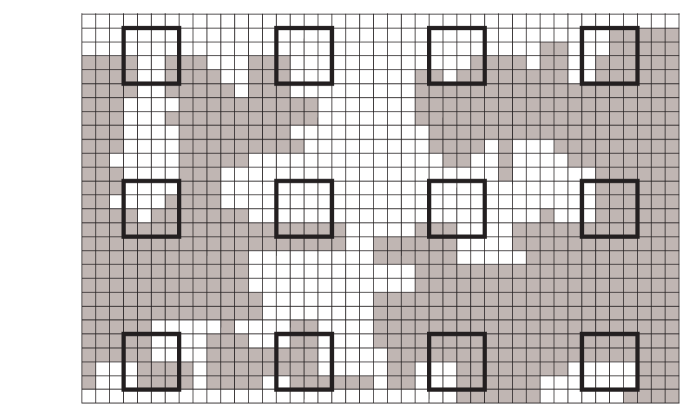
Figure 9.1: Possible illustration of $\Gamma$ and $\Delta$ in dual perspective when $k=4$ and $n=11$: the shaded squares are elements of $\Gamma$, squares inside $4\times 4$ boxes are elements of $\Delta$, vertices on boundaries of these boxes are members of $\tilde{\Delta}$. The infinite path $P_{\Gamma}$ is the boundary between $\Gamma$ and its complement.

We can think of the path $P_{\Gamma}$—which is a sequence of square faces of $\mathbb{Z}^{2}$ (or equivalently, a sequence of vertices in the dual graph)—as being oriented in such a way that $\Gamma$ lies on its left. Denote by $A(v)$ the event that $P_{\Gamma}$ hits $\tilde{\Delta}_{v}$, and in between the first and last times $P_{\Gamma}$ hits $\tilde{\Delta}(v)$, $P_{\Gamma}$ hits no square which is fewer steps away from a $\tilde{\Delta}(w)$, with $w\not=v$, than it is from $\tilde{\Delta}(v)$. For example, $A(v)$ occurs whenever $\Delta(v)$ is one of the $4\times 4$ boxes in Figure 9.1 except when $\Delta(v)$ is the top left box.

Clearly, by choosing $n$ large enough so that the probability that $P_{\Gamma}$ takes more than $n-k$ steps between visits to $\tilde{\Delta}(v)$ is small, we can make the probability of $A_{\infty}\backslash A(v)$ arbitrarily small.

We will henceforth assume that in additional to satisfying $n>2k$, we also have that $n\mathbb{Z}^{2}\subset\mathcal{L}$ and that $n$ is large enough so that $\rho(A(0))>\rho(A_{\infty})-\epsilon$. The $\mathcal{L}$-invariance of the law of the path $P_{\Gamma}$ implies that $\rho(A(v))>\rho_{k}(A_{\infty})-\epsilon$ for any $v\in\mathbb{Z}^{2}$; or equivalently, $\rho(A_{\infty}\backslash A(v))<\epsilon$. The values of $n$, $k$, and $\epsilon$ will remain fixed throughout the proof.

Given the event $A(v)$, we define $v_{+}$ and $v_{-}$ to be such that $\tilde{\Delta}(v_{-})$ is the last band that the path $P_{\Gamma}$ hits before the first time it hits $\tilde{\Delta}(v)$. Similarly, $\tilde{\Delta}(v_{+})$ is the first band that the path $P_{\Gamma}$ hits after the last time it hits $\tilde{\Delta}(v)$.

Let $C(v,w)$ be the event that some vertex incident to $\overline{\Delta}(v)$ and some vertex incident to $\overline{\Delta}(w)$ are in the same connected component of $\Gamma\backslash\Delta$. In other words, $C(v,w)$ is the event that there is a path in $\Gamma$ that connects vertices incident to $\overline{\Delta}(v)$ and $\overline{\Delta}(w)$ without passing through any other box $\Delta(x)$, $x\not\in\{v,w\}$. Given that $A(w)$ occurs, it is easy to see that $C(w,w_{+})$ (respectively, $C(w,w_{-})$) must occur as well—we see this by taking a path comprised of vertices that lie immediately to one side of the portion of $P_{\Gamma}$ that connects $\tilde{\Delta}(w)$ and $\tilde{\Delta}(w_{+})$ (respectively, $\tilde{\Delta}(w_{-})$).

Given a non-self-intersecting path $p=v_{1},\ldots,v_{r}$ in $\Gamma\backslash\Delta$ connecting $\overline{\Delta}(v)$ and $\overline{\Delta}(w)$, we define a continuous, non-self-intersecting path $\overline{p}$ from $nv$ to $nw$ by connecting the dots in the sequence $nv,v_{1},\ldots,v_{r},nw$ with straight line segments. Since $v_{1}\in\overline{\Delta}(v)\backslash\Delta(v)$ and $v_{r}\in\overline{\Delta}(w)\backslash\Delta(w)$ are initial and final points of $p$, it is not hard to see the the initial and final segments of $\overline{p}$ do not intersect any of the other segments. Given any continuous path $q$ from $nv$ to $nw$ which is contained (except for its two endpoints) in $\mathbb{R}^{2}\backslash n\mathbb{Z}^{2}$, we denote by $C_{q}(v,w)$ the event that there exists a path $p$ in $\Gamma\backslash\Delta$, connecting $\overline{\Delta}(v)$ and $\overline{\Delta}(w)$ for which $\overline{p}$ is homotopically equivalent to $q$ (i.e., there exists a continuous $Q:[0,1]^{2}\rightarrow\mathbb{R}^{2}$ with $Q(t,0)=\overline{p}(t)$, $Q(t,1)=q(t)$, $q(0,t)=v$, $q(0,t)=w$, for all $t\in[0,1]$ and $Q(t,u)\in\mathbb{R}^{2}\backslash\mathbb{Z}^{2}$ for all $(t,u)\in(0,1)\times[0,1]$). Denote by $C^{+}_{q}(v,w)$ the event that $w=v_{+}$ and the path $P_{\Gamma}$ from $\overline{\Delta}(v)$ to $\overline{\Delta}(w)$ is homotopic to $q$. Define $C^{-}_{q}(v,w)$ analogously using $v_{+}$ instead of $v_{-}$. Clearly, $C^{+}_{q}(v,w)$ and $C^{-}_{q}(v,w)$ are both contained in the event $C_{q}(v,w)$.

Let $B(v)$ be the event that there exists a cycle in $\Gamma\backslash\Delta$ which disconnects $\Delta(v)$ from infinity. We will ultimately prove Theorem 9.3.1 by showing, first, that certain combinations of events of the form $C_{q}(v,w)$ together imply, for topological reasons, the event $B(0)$; we then bound the probabilities of these combinations of events using the FKG inequality and the shift-invariance of the law of $P_{\Gamma}$. This will enable us to prove that $\rho(B(0))>\epsilon$, a contradiction.

Our next step is to review some basic facts about the topology of the countably punctured plane.

9.4.2 Homotopy classes of paths in countably punctured plane

It is well known that the homotopy group of $\mathbb{R}^{2}$ minus a discrete set of points is given by the free group generated by those points. (See, e.g., Section 3.5 and Exercise 3.4 of [69].) Instead of dealing with $\mathbb{R}^{2}\backslash\mathbb{Z}^{2}$, however, it will be convenient for us to deal with the closed countably punctured plane defined as follows. First, consider an closed annulus of inner radius $\epsilon$ and outer radius $\epsilon/2$. We can map this onto bijectively onto the space $D^{\prime}=D_{\epsilon}\backslash 0\cup 0\times S^{1}$, where $D_{\epsilon}$ is the closed disc of radius $\epsilon$ and $S^{1}$ is the unit circle, by sending a point $(r,\theta)$ (defined in polar coordinates) to $(2r-r_{0},\theta)$, if $r\neq 0$, and to $0\times\theta$ if $r=0$. We endow $D^{\prime}$ with the topology that makes $D^{\prime}$ and the annulus homeomorphic (when the annulus is endowed with the standard topology induced by the Euclidean metric).

We define the closed countably punctured plane $W=\mathbb{R}^{2}\backslash\mathbb{Z}^{2}\cup\mathbb{Z}^{2}\times S^{1}$ analogously. It is homeomorphic to $\mathbb{R}^{2}\backslash[\mathbb{Z}^{d}+D]$ (where $D$ is a closed disc of any radius less than $1/2$), and it is not hard to see that it has the same homotopy group as $\mathbb{R}^{2}\backslash\mathbb{Z}^{2}$. Intuitively, the closed countably punctured plane is obtained by first poking a hole in $\mathbb{R}^{2}$ at each lattice point and then inserting and infinitesimal rivet at that point; an advantage of that this space has over $\mathbb{R}^{2}\backslash\mathbb{Z}^{2}$ is that (as we will see later—see Figure 9.2, in the next section) every homotopy class has a minimal length representative.

We will now describe the homotopy group of $W$ more explicitly. Let $a=(a_{1},a_{2})$ be an arbitrary point in $\mathbb{R}^{2}\backslash\mathbb{Z}^{2}$ with irrational coordinates. For each $x$ in $\mathbb{Z}^{2}$, let $r_{x}$ be the closed line segment from $a$ to the point $x$ (including its limit point $x\times\arg(a-x)$). Let $u_{x}$ be the portion of the same ray (from $a$ through $x$ to infinity) which lies between $x$ and $\infty$, together with its limit point $x\times\arg(x-a)$.

We can describe the homotopy classes of paths in $\mathbb{R}^{2}\backslash\mathbb{Z}^{2}$ which start and end at $a$ in the following way. Let $\overline{x}$ be the homotopy class of a path which follows $r_{x}$ from $a$ towards $x$, then makes a counterclockwise loop around $x$, and then returns to $a$ along $r_{x}$. Every homotopy class can be uniquely represented by a reduced word in elements of the form $\overline{x}$, for $x\in\mathbb{Z}^{2}$ (i.e., a finite-length word in the elements $\overline{x}$ and $\overline{x}^{-1}$ in which no element $\overline{x}$ appears next to its inverse $\overline{x}^{-1}$).

Now, let $p:[0,1]\mapsto\mathbb{R}^{2}$ be any cycle in $\mathbb{R}^{2}\backslash\mathbb{Z}^{2}$ which starts and ends at $a$ and which has only finitely many intersections with the rays $u_{x},x\in\mathbb{Z}^{2}$. Given $p$, we can generate the word corresponding to its homotopy class as follows. Let $t$ vary between $0$ to $1$. Each time $p(t)$ crosses a ray $u_{x}$ in a counterclockwise direction, add $\overline{x}$ to the end of the word; each time it crosses a ray $u_{x}$ in a clockwise direction, add $\overline{x}^{-1}$. The reader may easily verify (e.g., using induction on word length) that the fundamental group element produced in this way describes the homotopy class of $p$.

Through the remainder of our discussion, if $x\in\mathbb{Z}^{2}$, we will treat $x$ as an element of $W$ by using $x$ as a shorthand for $x\times 0$. For any $x,y\in\mathbb{Z}^{2}$, let $P_{x,y}$ be the set of continuous paths from $x$ to $y$ in $W$. Let $r_{x}^{\prime}$ denote the linear segment from the $a$ to $x\times\arg(a-x)$, followed by a counter-clockwise arc from $x\times\arg(a-x)$ to $x\times 0$. Note that the map $p\mapsto(r^{\prime}_{x})^{-1}pr^{\prime}_{y}$ (using the standard concatenation definition of path multiplication; see, e.g., Chapter 2 of [69]) induces a one-to-one correspondence between homotopy classes of paths $p$ from $a$ to itself and homotopy classes of paths from $x$ to $y$. (The inverse of this map is given by $p\mapsto r^{\prime}_{x}p(r^{\prime}_{y})^{-1}$.)

We can each view $p\in P_{x,y}$ as a function from $[0,1]$ to $W$, defined up to a monotonic, continuous reparametrization of $[0,1]$; by slight abuse of notation, we will sometimes also use $p$ to denote the subset of $W$ contained in the image of $[0,1]$ under this function. If $p\in P_{x,y}$ for some $x$ and $y$, let $P_{p}$ be the set of paths in $P_{x,y}$ which are homotopically equivalent to $p$ in $W$. Let $P$ be the union of $P_{x,y}$ over all disjoint pairs $x,y\in\mathbb{Z}^{2}$.

9.4.3 Minimal length paths

For which sets of paths $p_{1},\ldots,p_{k}$ and points $x\in\mathbb{Z}^{2}$ is it the case that $x$ lies in a bounded component of $\mathbb{R}^{2}\backslash\cup_{i=1}^{k}q_{i}$ for every $(q_{1},\ldots,q_{k})\in\prod_{i=1}^{k}P_{p_{i}}$? Roughly speaking, the answer is that this is the case whenever the “taut” or “minimal length” paths

$$(\tilde{p}_{1},\tilde{p}_{2},\ldots,\tilde{p}_{k})\in\prod_{i=1}^{k}P_{p_{i}}$$

in these homotopy classes disconnect $x$ from infinity in a certain “strong” sense. The purpose of this subsection is to make this statement precise. Some of the results in this section are related to algorithms in the computer science literature for finding minimal length paths of given homotopy classes in regions with polygonal obstacles (see, e.g., [54] for examples and additional references) and for testing equivalency between homotopy classes by computing the unique minimal length representatives of those classes. However, we have been unable to find exactly what we need in the literature, so we will give our own proofs of some of the basic facts (such as the existence of paths of minimal length) in our context.

A line segment in $W$ is an open line segment in $\mathbb{R}^{2}\backslash\mathbb{Z}^{2}$ together with its limit points (which may be in $\mathbb{Z}^{2}\times S^{1}$). An arc in $W$ is a closed path in $x\times S^{1}$ (for some $x\in\mathbb{Z}^{2}$) which moves either strictly clockwise or strictly counterclockwise around $S^{1}$. A piecewise linear path $p$ in $W$ is a path formed by concatenating finitely many line segments and arcs (where no two arcs appear sequentially in the concatenation); we will also assume that $p$ is parametrized in such a way that it is not constant on any interval of $[0,1]$. It also suits our purposes to assume that the endpoints of $p$ are points of $\mathbb{Z}^{2}$.

When $p$ is piecewise linear, we write $p^{\prime}_{+}$ for the right derivative and $p^{\prime}_{-}$ for the left derivative of $p$ (so that $p^{\prime}_{+}(t)=p^{\prime}_{-}(t)$ whenever $p$ is differentiable at $t$). If, in some subinterval interval of $[0,1]$, we have $p(t)=(x,\theta(t))$, with $x\in\mathbb{Z}^{2}$, then we write $p^{\prime}(t)=\frac{\partial}{\partial t}\theta(t)(-\sin\theta,\cos\theta)$; we think of $p^{\prime}(t)$ as a vector pointing “around the infinitesimal circle” in the direction that $p$ is moving; we define $p^{\prime}_{+}(t)$ and $p^{\prime}_{-}(t)$ on such subintervals accordingly. If $p(0)=(x_{0},\theta_{0})$, then we write $p^{\prime}_{-}(0)=(-\cos\theta_{0},-\sin\theta_{0})$, and if $p(1)=(x_{1},\theta_{1})$, we write $p^{\prime}_{+}(1)=(-\cos\theta_{1},-\sin\theta_{1})$. (Informally, we think of $p$ as “emerging from inside the hole at $x_{0}$” when $t=0$ and “turning inwards into the hole at $y_{0}$” when $t=1$.) Now, whenever $p$ is piecewise linear, $p^{\prime}_{+}$ and $p^{\prime}_{-}$ are defined throughout the interval $[0,1]$. Unless otherwise stated, we will always assume that a piecewise linear $p$ is parametrized according to Euclidean length/arc length (so that $|p^{\prime}_{-}|$ and $|p^{\prime}_{+}|$ are both constant). Also, we will assume that $p$ has no $U$-turns (i.e., points $t$ at which $p^{\prime}_{-}(t)=p^{\prime}_{+}(t)$.)

If $p$ is piecewise linear, a free corner of $p$ is a point $t\in[0,1]$ for which $p(t)\in\mathbb{R}^{2}\backslash\mathbb{Z}^{2}$ and at which the path $p$ changes directions; we refer to $p(t)$ as the position of the corner. We also refer to each connected component of $p^{-1}[\mathbb{Z}^{2}\times S^{1}]$ as a loop corner of $p$; the length of a loop corner is the length of the corresponding arc; the position is the corresponding point $x\in\mathbb{Z}^{2}$. We say $p$ is taut if it contains no free corners and the length of every loop corner is at least $\pi$. The length of a piecewise linear path in $W$ is the sum of the Euclidean lengths of its line segments. We now prove the following:

Lemma 9.4.1

In every homotopy class $P_{p}\subset P_{x,y}$ there exists exactly one taut path $\tilde{p}$. This $\tilde{p}$ has minimal length among all paths in $P_{p}$.

• Although this lemma may seem obvious intuitively, it will take us a fair amount of space to prove it. Suppose that $q_{1}$ and $q_{2}$ are two distinct homotopically equivalent taut paths in $P_{p}\subset P_{x,y}$. Choose $a$ to be a generic point with irrational coordinates that lies vertically below the entire paths $q_{1}$ and $q_{2}$—i.e., the second coordinate of $a$ is less than the smallest value $x_{2}$ which occurs in a point $(x_{1},x_{2})$ in either of these paths; in particular, this allows us to assume that whenever $x\in\mathbb{Z}^{2}$ and $\overline{x}$ occurs in the word corresponding to $P_{p}$, $x$ is higher than (i.e., has higher second coordinate than) the point $a$ in the plane $\mathbb{R}^{2}$.

  

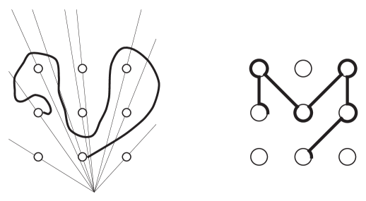
  Figure 9.2: A path $p$ (left) and the taut version $\tilde{p}$ (right). The infinitesimal “rivets” are of $W$ are shown as small circles on the left, slightly larger circles on the right. Rays $r(x)$ and $u(x)$ are depicted on the left.

Now, for $q_{1}$, we can form a word as follows. Let $X$ be the finite set of points $x$ for which one of the paths $q_{i}$ either crosses $u_{x}$ at some point or contains a loop corner at position $x$. Order the points $x_{1},x_{2},\ldots,x_{m}$ in order of the arguments of $(x-a)$. Let $t$ vary between $0$ to $1$. Each time $q_{1}(t)$ crosses a ray $u_{x}$, with $x\in X$, in a counterclockwise direction, add $\overline{x}$ to the end of the word; each time it crosses such a ray $u_{x}$ in a clockwise direction, add $\overline{x}^{-1}$. Similarly, each time it cross $r_{x}$, with $x\in X$, counterclockwise, add $\hat{x}$ to the end of the word; each time it crosses such an $r_{x}$ clockwise, add $\hat{x}^{-1}$ to the end of the word. Denote this word by $w_{1}$ and the analogously defined word for $q_{2}$ by $w_{2}$. (Since $a$ is generic, and each of $q_{1}$ and $q_{2}$ contains only finitely many arcs and line segments, it is not hard to see that that the set of $t$ at which one of the $q_{i}(t)$ crosses a given $u_{x}$ or $r_{x}$ is finite, and that at each such $t$, the path crosses the ray transversely—either clockwise or counterclockwise—so that the above construction is well defined.)

The rays $r_{x_{i}}\cup u_{x_{i}}$ separate $W$ into wedge shaped open pieces; for $1\leq i\leq m-1$, denote by $W_{i}$ the piece between $r_{x_{i}}\cup u_{x_{i}}$ and $r_{x_{i+1}}\cup u_{x_{i+1}}$. Denote by $W_{0}=W_{m}$ the complement of the closures of the $W_{i}$ for $1\leq i\leq m-1$. Note that we write down a symbol $\overline{x}_{i}$ or $\hat{x}_{i}$ each time $q_{1}$ passes from $W_{i}$ to $W_{i+1}$ and $\overline{x}_{i}^{-1}$ or $\hat{x}_{i}^{-1}$ each time $q_{i}$ passes from $W_{i+1}$ to $W_{i}$. Now, we observe that if $q_{1}$ is taut, no two symbols of the form $\overline{x}_{i}$ and $\overline{x}_{i}^{-1}$ (or, similarly, $\hat{x}_{i}$ and $\hat{x}_{i}^{-1}$) can occur in sequence. If they did, then there would be some $t_{1}$ and $t_{2}$ with $q_{1}((t_{1},t_{2}))$ contained in $W_{i}$ while $q_{1}(t_{1})$ and $q_{1}(t_{2})$ both belong to the same member of $\{r_{x_{i}},u_{x_{i}}\}$. And it is easy to see that at some point in this interval $(t_{1},t_{2})$ (e.g., the first point at which the argument of $q_{1}$ achieves its maximum) $q_{1}$ must have either a loop corner at $x_{i+1}$ (with length less than $\pi$) or a free corner. A similar argument implies that the opposite sequences $\hat{x}_{i}^{-1}\hat{x}_{i}$ and $\overline{x}_{i}^{-1}\overline{x}_{i}$ cannot occur in either $w_{1}$ or $w_{2}$.

Since symbols occur when $q_{i}$ passes from one wedge to another, it follows that whenever a positive symbol ($\overline{x}_{i}$ or $\hat{x}_{i}$) and an inverse of a symbol (of form $\overline{x}_{i}^{-1}$ or $\hat{x}_{i}^{-1}$) occur next to each other in the word, then they have the same index $i$ and one is a “hat” and one is a “bar” symbol. Also, it is easy to see that if two positive symbols occur successively in $w_{1}$, and the index of the first is $i$, then the index of the second is $i+1$. If two negative symbols occur successively and the index of the first is $i$, then the index of the second is $i-1$.

We know that the elements of the form $\overline{x}_{i}$ and $\overline{x}^{-1}$ that appear in the word are determined by the homotopy class of $p$. From the above paragraph, it is clear that $\overline{x}_{i}$ and its inverse $\overline{x}_{i}^{-1}$ cannot appear in the word with only “hat” elements separating them; otherwise, a hat symbol would have to occur next to its inverse. It follows that, if the “hat” symbols are omitted, then the remaining “bar” symbols give a reduced form expression of the fundamental group word of $p$. Also, in between a pair of “bar” symbols, the hat symbol sequence is completely determined by the rules of the above paragraph. Thus, $w_{1}=w_{2}$.

Now, let $f_{1}(i)$ be points where $q_{1}$ first intersects the ray that corresponds to the $i$th element of the word. Since $q_{1}$ is taut, each $f_{1}(i)$ is either a point $x$ in $\mathbb{Z}^{2}$—at which a loop corner of arc length at least $\pi$ occurs—or at a point in the interior of $r_{x}$ or $u_{x}$. Define $f_{2}$ accordingly. It is not hard to see that each pair $f_{1}(i)$ and $f_{1}(i+1)$ must be connected by a straight line segment and/or arc of $q_{1}$ (since the pair is connected by a piecewise linear path which intersects no ray transversely and has no corners); it follows that if $f_{1}$ = $f_{2}$, then $q_{1}$ and $q_{2}$ must be equal. In fact, if $f_{1}(i)\in\mathbb{Z}^{2}$, then its argument is determined by the word ordering; thus, $f_{1}(i)$ is determined by the value $g_{1}(i)=|f_{1}(i)-a|$. So it is enough for us to prove that $g_{1}(i)=g_{2}(i)$ for all $i$. Suppose otherwise, and let $i$ be a value for which $g_{1}(i)-g_{2}(i)$ is maximal. Suppose that $f_{1}(a)$ and $f_{2}(a)$ lie along the ray through $x_{j}$. If neither lies at the point $x_{j}$, then a corner cannot occur at either one of them, and a simple geometric argument shows that at least one of the values $g_{1}(i-1)-g_{2}(i-1)$ and $g_{1}(i+1)-g_{2}(i+1)$ is greater than $g_{1}(i)-g_{2}(i)$. On the other hand, suppose that only $f_{1}(i)$ lies at the point $x_{j}$ and $f_{2}(i)$ does not. Assume for simplicity that $f_{1}(i)$ and $f_{2}(i)$ lie on $u_{x}$ (the case when they lie on $r_{x}$ is similar). Then we see, first, since $f_{2}(i)$ is part of a straight line segment of $q_{2}$ from the ray through $x_{j-1}$ to the ray through $x_{j+1}$, the values $f_{2}(i+1)$ and $f_{2}(i-1)$ will lie on this pair of rays, as will $f_{1}(i+1)$ and $f_{1}(i-1)$ (since the words are equivalent). It follows that the corner that occurs in $q_{1}$ at $f_{1}(i)$ has angle between $\pi$ and $2\pi$ (if it were greater than $2\pi$, then the path would have to intersect $r_{x}$ before proceeding one of the other rays). Again, a simple geometric argument implies at least one of the values $g_{1}(i-1)-g_{2}(i-1)$ and $g_{1}(i+1)-g_{2}(i+1)$ is greater than $g_{1}(i)-g_{2}(i)$. We have now proved that the class $P_{p}\subset P_{x,y}$ contains at most one taut path $\tilde{p}$.

It remains to prove that $P_{x,y}$ contains at least one taut path $\tilde{p}$ and that this path has minimal length. Given a word $w$, the above arguments determine the order in which any taut path in the corresponding homotopy class from $x$ to $y$ would have to intersect $r_{x_{i}}$ and $u_{x_{i}}$ (and the direction—clockwise or counterclockwise) for each such value). Let $P_{w}$ be the set of paths from $x$ to $y$ which indeed intersect the rays in the given order; as seen above, such paths are completely determined by the function $g_{i}$. Since length is a continuous function of the $g_{i}$, it is clear that $P_{w}$ contains an element $\tilde{p}$ for which the length is minimal. It is not hard to see that if $\tilde{p}$ failed to be taut, we could decrease its length by moving one of the $g_{i}$.

How do we see that $\tilde{p}$ has minimal length among all paths? Arguments similar to those above imply that when looking for minimal length paths, we may restrict our attention to paths $p$ which induce the same word $w$ as $\tilde{p}$ (as described above). (If this is not the case, then a portion of the path will exit and enter one of the wedges $W_{i}$ along the same ray; and thus the path can be shortened by pulling that portion taut.) It is also not hard to see that we may assume $p$ is piecewise linear (since otherwise, by “straightening” segments and arcs of $p$, we could produce a piecewise linear $p^{\prime}\in P_{p}$ with length less than or equal to that of $p$). The arguments above then imply that $\tilde{p}$ has minimal length among paths of this form; hence it has minimal length over all all paths in $P_{p}$.   

If $r$ is a path, each of whose endpoints is an endpoint of either $q$ or $p$, then we say that $p$ and $q$ have a crossing of type $r$ if there is a path $r^{\prime}\in P_{r}$ for which the image of $r^{\prime}$ in $W$ lies in the union of the images of $p$ and $q$. Now define a metric on the set of paths in a particular homotopy class: $\delta(p,q)=\inf\left(\sup_{t\in[0,1]}|p^{\prime}(t)-q^{\prime}(t)|\right)$, where $|x|$ denotes the Euclidean norm of $x$ and the infimum runs over all parametrizations $p^{\prime}$ and $q^{\prime}$ of the paths $p$ and $q$. We say two paths $p_{1}$ and $p_{2}$ are equivalent if $\delta(p_{1},p_{2})=0$; so $\delta$ is actually a metric on equivalence classes, not paths. Denote by $B_{\gamma}(p)$ the ball of radius $\gamma$ about $p$ in this metric. We say that $p$ and $q$ have an essential crossing of type $r$ if for some sufficiently small $\gamma$, $p^{\prime}$ and $q^{\prime}$ have a crossing of type $r$ whenever $(p^{\prime},q^{\prime})\in\left(P_{p}\cap B_{\gamma}(p),P_{q}\cap B_{\gamma}(q)\right)$. See Figure 9.3. The usefulness of these concepts stems from the following lemma.

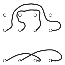
Figure 9.3: The taut versions of the upper two paths have points of intersection but do not have an essential crossing; the taut versions of the lower two paths have an essential crossing.

Lemma 9.4.2

If $p_{1}$ and $p_{2}$ are piecewise linear paths and $\tilde{p}_{1}$ and $\tilde{p}_{2}$ have an essential crossing of type $r$, then $p_{1}$ and $p_{2}$ also have an essential crossing of type $r$.

• From the definition of essential crossings, it is clear that the set $C_{r}$ of path pairs $(q_{1},q_{2})\in P_{p_{1}}\times P_{p_{2}}$ with no essential crossings of type $r$ is closed with respect to the product topology generated by $\delta$ on $P_{p_{1}}\times P_{p_{2}}$. It is also not hard to see that the set of elements in $P_{p_{1}}\times P_{p_{2}}$ with combined length less than $L$, for some $L\in\mathbb{R}$, is compact; in particular, the length function is lower semi-continuous. It follows that the length function achieves its minimum over $C_{r}$ on some pair: we may assume this pair is $(p_{1},p_{2})$.

  Now, we claim that $p_{1}$ and $p_{2}$ are both taut. Suppose otherwise, and that without loss of generality $p_{1}$ is not taut. Then there either exists an $s\in(0,1)$ for which $p_{1}(s)=x\in\mathbb{R}^{2}\backslash\mathbb{Z}^{2}$ and $p_{1}$ fails to be linear on a neighborhood of $s$, or there exists an $s\in[0,1]$ for which $p_{1}(s)=x\in\mathbb{Z}^{2}\times S^{1}$ and the angle of the arc at $p_{1}$ is less than $2\pi$.

  Now, let $D$ be a small closed disc centered at $x$; we may assume that $D$ contains no elements of $\mathbb{Z}^{2}$ (except $x$ if $x\in\mathbb{Z}^{2}$) and that its radius is generic—so that $p_{1}$ and $p_{2}$ each intersect the boundary of $D$ at only finitely many points.

  Let $q_{1}$ and $q_{2}$ be obtained from $p_{1}$ and $p_{2}$ by “pulling taut” the portions of $p_{1}$ and $p_{2}$ inside $D$, i.e., replacing them with the minimal length piecewise linear paths with the same endpoints on $D$ and in the same homotopy classes. Clearly, $q_{1}$ and $q_{2}$ are shorter than $p_{1}$ and $p_{2}$. We will be done if we can show that $q_{1}$ and $q_{2}$ (or some $q_{1}^{\prime}$ and $q_{2}^{\prime}$ whose length can be made arbitrarily close to the length of $q_{1}$ and $q_{2}$) have no essential crossing of type $r$.

  

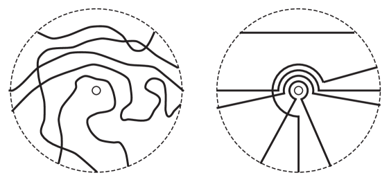
  Figure 9.4: Five paths pulled “almost taut.” Each pair of paths with a point of intersection on the right side must have an analogous point of intersection on the left side.

Now, by assumption, there exist $p_{1}^{\prime}$ and $p_{2}^{\prime}$ arbitrarily close to $(p_{1},p_{2})$ which have no crossing of type $r$. Given such $p_{1}^{\prime}$ and $p_{2}^{\prime}$, we claim that we can “almost pull taut” the portions of $p_{1}^{\prime}$ and $p_{2}^{\prime}$ inside of $D$ in such a way that no crossing occurs of type $r$ occurs. First let us deal with the case that $x$ is not a point in $\mathbb{Z}^{2}$; in this case, we simply pull $p_{1}^{\prime}$ and $p_{2}^{\prime}$ taut in $D$ to produce $q_{1}^{\prime}$ and $q_{2}^{\prime}$. Now observe that a pair of segments in $q_{1}^{\prime}$ and $q_{2}^{\prime}$ will intersect one another if and only if the positions at which the segments exit $D$ ordered in such a way that the endpoints of one segment divide the circle into two pieces, one containing each of the endpoints of the other segment (by adjusting $p_{1}^{\prime}$ and $p_{2}^{\prime}$ slightly if necessary, we may assume that their points of intersection with the boundary $\partial D$ occur at distinct locations).

The famous Jordan curve theorem states that any continuous simple closed curve in the plane separates the plane into two disjoint regions, the inside and the outside. A simple corollary is that if distinct points $a,b,c,d$ are in cyclic order around a disc, and $p$ is a continuous path in the disc from $a$ to $c$, and $q$ is a continuous path from $b$ to $d$, then $p$ and $q$ must intersect. It is not hard to see that if $q_{1}^{\prime}$ and $q_{2}^{\prime}$ have a crossing of type $r$, $p_{1}^{\prime}$ and $p_{2}^{\prime}$ will have a crossing of the same type. It follows by assumption that $q_{1}^{\prime}$ and $q_{2}^{\prime}$ have no crossing of type $r$. Finally, it is not hard to see (by choosing $p_{1}^{\prime}$ and $p_{2}^{\prime}$ close enough to $p_{1}$ and $p_{2}$) that we can arrange for $q_{1}^{\prime}$ and $q_{2}^{\prime}$ to be arbitrarily close, in the $\delta$ metric, to $q_{1}$ and $q_{2}$; hence, $q_{1}$ and $q_{2}$ have no essential crossing of type $r$.

The above argument shows that if $p_{1}$ and $p_{2}$ are minimal length paths with no essential $r$ crossing, then $p_{1}$ and $p_{2}$ must be taut in a neighborhood of any point $x\in\mathbb{R}^{2}\backslash\mathbb{Z}^{2}$. If $x\in\mathbb{Z}^{2}$, and either of $p_{1}$ or $p_{2}$ fails to be taut at $x$ (i.e., has an arc whose length is less than $\pi$) then we can apply a similar argument. In this case, to pull $p_{1}^{\prime}$ and $p_{2}^{\prime}$ “taut” we replace the segments of these paths passing through $D$ with the minimal length paths in the same homotopy class; a path of this type will either be a straight line segment connecting two points on $D$ or a straight line segment from the boundary of $D$ followed by an arc of length at least $\pi$ and another straight line segment out to the outer boundary of $D$.

Let $A$ be the set of all the arcs that occur in the paths of this form produced from the segments of $p_{i}^{\prime}$ and $q_{i}^{\prime}$. We can partially order these arcs via inclusion; it is well-known that every partial ordering has an extension to a total ordering, and hence, we can replace each infinitesimal arc with an arc with the same angle and small positive radius — and choose the radii in such a way that they are decreasing with respect to the total ordering. See Figure 9.4. Adjusting $p_{1}^{\prime}$ and $p_{2}^{\prime}$ slightly if necessary, we may assume that no two of these arcs share an endpoint.

It is clear that the paths defined in this way can be made to have arbitrarily small radius. Two such paths will cross one another if and only if the corresponding arcs $a_{1}$ and $a_{2}$ have the property that $a_{1}$ is neither a subset of $a_{2}$ nor a subset of its complement. Another corollary of the Jordan Curve Theorem is that if $\theta_{1}<\theta_{2}<\theta_{3}<\theta_{4}$ are angles and $D$ has radius $R$, and $p$ is a path in $D\backslash\{x\}$ from $(R,\theta_{1})$ to $(R,\theta_{3})$ (where the angles, elements of $\mathbb{R}$, may be viewed as determining points in the universal cover of the annulus—so that the amount of winding of $p$ is given by $\theta_{3}-\theta_{1}$) and $q$ is an analogously defined path from $(R,\theta_{2})$ to $(R,\theta_{4})$, then $p$ and $q$ must cross (and in fact, must have a crossing of the same type). As before, it is not hard to see that we can arrange for $q_{1}^{\prime}$ and $q_{2}^{\prime}$ to be arbitrarily close to $q_{1}$ and $q_{2}$; hence $q_{1}$ and $q_{2}$ have no essential crossing of type $r$.   

We say that a collection of piecewise linear paths $p_{1},\ldots,p_{k}$ separates $x$ from $y$ if there exists no path from $x$ to $y$ which does not cross at least one of the $p_{i}$. We say that $p_{1},\ldots,p_{k}$ essentially separate $x$ from $y$ if there exists no piecewise linear path from $x$ to $y$ which does not have an essential crossing with at least one of the $p_{i}$.

We say that $p_{1},\ldots,p_{k}$ (essentially) bound $x$ away from infinity if for all but finitely many $y$, $p_{1},\ldots,p_{k}$ (essentially) separates $x$ from $y$.

Lemma 9.4.3

If $\tilde{p}_{1},\tilde{p}_{2},\ldots,\tilde{p}_{k}$ essentially separate $x$ from infinity, then $p_{1},\ldots,p_{k}$ essentially separate $x$ from infinity. In particular, $p_{1},\ldots,p_{k}$ separate $x$ from infinity.

9.4.4 Completing proof of Theorem 9.3.1

Now, we return to the terminology of Section 9.4.1. We have already defined an extremely small constant, $\epsilon$. We will also need $\delta$ (a very small constant) and $\gamma$ (a quite small constant) and $\beta$ (a small constant). The exact values are unimportant. The following will comfortably suffice for our purposes:

$$\epsilon=10^{-10000}\mu(A_{\infty})^{10000}$$

$$\delta=10^{-1000}\mu(A_{\infty})^{1000}$$

$$\gamma=10^{-100}\mu(A_{\infty})^{100}$$

$$\beta=10^{-10}\mu(A_{\infty})^{10}$$

Recall that our aim is to prove that $\rho(B(0))\geq\epsilon$, thereby deriving a contradiction.

We call $w$ a $\delta$-preferred direction if the coordinates of $w$ are relatively prime to one another and $\rho(C_{p_{v}}(v,v+w))\geq\delta$ for all $v\in\mathbb{Z}^{2}$ where $p_{v}$ is a straight path connecting $v$ to $v+w$.

Lemma 9.4.4

If there exist two distinct $\delta$-preferred directions $w_{1}$ and $w_{2}$ (with $w_{1}\not=-w_{2}$), then $\rho(B(0))\geq\epsilon$.

• The FKG inequality implies that with probability at least $\delta^{8}$, the events $C_{p_{i}}(a_{i},a_{i+1})$ occur for each $1\leq i\leq 8$, where the values $a_{i}$ are given by $v,v+w,w,-v+w,-v,-v-w,-w,v-w,v$ (so $a_{9}=a_{1}$), successively, and each $p_{i}$ is the straight path from $a_{i}$ to $a_{i+1}$. In this case, there are eight paths—call them $q_{1},\ldots,q_{i}$ contained in $\Gamma\backslash\Delta$—with each $q_{i}$ connecting $\overline{\Delta}(a_{i})$ to $\overline{\Delta}(a_{i+1})$ in a way homotopically equivalent $p_{i}$.

  We claim that if each of these events occurs and $A(a_{i})$ occurs for each $i$, then $B(0)$ must also occur. To see this, first, say a vertex $b\overline{\Delta}(v)\cap\Gamma$ is exposed if there exists a path in $\Gamma\backslash\Delta$ connecting $b$ to some $b^{\prime}\in\overline{\Delta(w)}$, for some $w\not=v$. Then observe that if a given $A(v)$ occurs, then any two exposed points in $\overline{\Delta}(v)$ can be connected by a “short” path in $\overline{\Delta}(v)$—i.e., a path which contains only points that are closer to $\Delta(v)$ than to any other $\Delta(w)$. If $v\not=0$, then such a path is homotopically retractable in $\mathbb{R}^{2}\backslash\{(0,0)\}$ to a straight line (since $v\not=0$). By concatenating these short paths with the $q_{i}$’s, we produce a cycle in $\overline{\Delta}(a_{i+1})$ in $\Gamma\backslash\Delta$ which is homotopically equivalent in $\mathbb{R}^{2}\backslash\{(0,0)\}$ to the concatenation of the $p_{i}$’s (which surrounds $0$). It follows that $B(0)$ must occur.

  Given the events $C_{p_{i}}(a_{i},a_{i+1})$—which imply the event $A_{\infty}$—the $A(a_{i})$ fail to occur with $\rho$ probability at most $8\epsilon$. Thus, $\rho(B(0))\geq\delta^{8}-8\epsilon\geq\epsilon$.   

Lemma 9.4.5

There exists at least one $\gamma$-preferred direction.

• We will assume that there is no $\gamma$-preferred direction, and attempt to derive a contradiction. Now, let $u(v)$ be the angle of the direction of the first line segment in the taut path with the same homotopy class as the path $P_{\Gamma}$ assumes between $v$ and $v_{+}$ (this is well-defined given the event $A(v)$). Given two distinct angles $(\theta_{1},\theta_{2})$, let $C_{(\theta_{1},\theta_{2})}(v)$ be the event that $C_{p}(v,w)$ occurs for some path $p$ which, when pulled taut, leaves $v$ in a direction which lies strictly in the interval $(\theta_{1},\theta_{2})$ (on the counterclockwise side of $\theta_{1}$).

  Now suppose that with probability at least $\beta$, $u(0)$ lies in $(0,\pi/2)$ and with probability at least $\beta$ it lies in $(\pi/2,\pi)$; by shift-invariance of the law of $P_{\Gamma}$, this implies the same is true of $u(v)$ for any $v$. This also implies that for each $v$, the increasing events $C_{(0,\pi/2)}(v)$ and $C_{(\pi/2,\pi)}(v)$ occur with probability at least $\beta$. Hence their union occurs with probability at least $\beta^{2}$. Now, we claim that $C_{0,\pi/2}((0,0))$ and $C_{\pi/2,\pi}((1,0))$ together imply $C_{p_{0}}((0,0),(1,1))$where $p_{0}$ is the straight path from $(0,0)$ to $(1,0)$. To see this, first make the geometric observation that any taut path from $(0,0)$ with starting direction in $(0,\pi/2)$ and a taut path from $(1,0)$ with starting direction in $(\pi/2,\pi)$ must intersect; in fact, the first linear segments of these two paths must cross transversely at some point in the set $\{(x_{1},x_{2}):0<x_{1}<1\}$, forming an essential crossing of type $p_{0}$. Lemma 9.4.2 then implies that $C_{p_{0}}((0,0),(1,1))$ follows from $C_{0,\pi/2}((0,0))$ and $C_{\pi/2,\pi}((1,0))$. Thus, in this case, $(1,0)$ is a $\beta^{2}>\gamma$-preferred direction. Using similar arguments for $(0,1)$, we conclude that no two consecutive quadrants can each contain $u(0)$ with probability $\beta$.

  The same argument applies if we replace $(1,0)$ and $(0,1)$ with any pair of generators for the lattice $\mathbb{Z}$ (i.e., any pair of vectors $w_{1}$ and $w_{2}$, whose integer span is $\mathbb{Z}^{2}$, or equivalently, any $w_{1}$ and $w_{2}$, each of which contains a relatively prime pair of coordinates, for which the parallelogram with sides determined by $w_{1}$ and $w_{2}$ has unit area). In this case, we cannot have $u(0)$ contained in two consecutive quadrants of the form $(\arg(\pm v),\arg(\pm w))$ each with $\beta$ probability. This also implies that at least one pair of opposite quadrants has combined probability less than $2\beta$.

  Now, suppose that $u(0)$ is equal to $\pi/2$ with probability $\beta$. When this occurs, the taut version $\tilde{p}$ of the section of $P_{\Gamma}$ between $(0,0)$ and $(0,0)_{+}$ will start in the $(0,1)$ direction and pass the points $(0,1),(0,2),(0,3),\ldots$ (on either the left or right, with arcs of length $\pi$) up to some vertex at which it either turns to the left or right or ends. Assume without loss of generality that with probability at least $\beta/2$, $\tilde{p}$ does not pass the first vertex on the right with angle $\pi$. Conditioned on this event, let $i$ denote the first $(0,i)$ in the sequence that $\tilde{p}$ does not pass on the left (with angle $\pi$ or greater—see Figure 9.5). This $i$ is a random variable; let $i_{0}$ be its median value (conditioned on $u(0)$ and on $\tilde{p}$ not passing the first vertex on the right with angle $\pi$). Now, let $C_{i_{0}}^{+}(v)$ be the event that there is some path $p$ in $\Gamma\backslash\Delta$ between $\tilde{\Delta}(v)$ and some $\tilde{\Delta}(w)$, which, when pulled taut starts out by moving in the $(0,1)$ direction (as before, not passing first vertex on the right at angle $\pi$) and passes at least $i_{0}$ vertices on the left before it stops or turns; let $C_{i_{0}}^{-}(v)$ be defined analogous except that the taut path passes at most $i_{0}$ vertices on the left before it stops or turns. Each of these events has probability at least $\beta/4$. Now, we claim that $C_{i_{0}}^{+}((0,0))$ and $C_{i_{0}}^{-}(0,1)$ together imply $C_{p_{0}}((0,0),(0,1))$, where $p_{0}$ is the straight path from $(0,0)$ to $(0,1)$. To see this, as before, by Lemma 9.4.2, it is enough to let $p_{1}$ and $p_{2}$ be the paths whose existence is guaranteed by the events $C_{i_{0}}^{-}((0,0))$ and $C_{i_{0}}^{+}(0,1)$ and to show that $\tilde{p}_{1}$ and $\tilde{p}_{2}$ must have an essential crossing of type $p_{0}$. (We leave these details to the reader.) It follows that $(0,1)$ is a $(\beta/4)^{2}>\gamma$-preferred direction. We conclude that $u(0)$ cannot be equal to $(0,1)$ with probability $\beta$; a similar argument implies that $u(0)$ cannot be equal to any single vector $v$ with probability $\beta$.

  

  Figure 9.5: If the bottom vertex is the origin, then the first path shown passes two vertices (namely, $(0,1)$ and $(0,2)$ on the left). The other two paths each pass one vertex on the left.

Now, with probability $A_{\infty}$, $u(0)$ has some direction. Thus, for any pair of generators $(v,w)$, since each of $\pm v$ and $\pm w$ has probability less than $\beta$, and one pair of opposite quadrants has combined probability less than $2\beta$, the other pair of opposite quadrants must have combined probability equal to at least $A_{\infty}-6\beta$. Assume without loss of generality that $u(0)$ lies in the intervals $(\arg v,\arg w)$ and $(\arg(-v),\arg(-w))$ with probability at least $A_{\infty}-6\beta$. Equivalently, $u^{\prime}(0)\in(\arg v,\arg w)$ where $u^{\prime}(0)$ is $u(0)$ modulo $\pi$.

Now, we can replace $v,w$ with either the set of generators $(v,v+w)$ or $(v+w,w)$. Since $u$ is equal to $\pm(v+w)$ with probability at most $\beta$, we have that $u^{\prime}(0)$ will lie in one of the two intervals $(\arg v,\arg(v+w))$ and $(\arg(v+w),\arg w)$ with probability at least $(A_{\infty}-7\beta)/2$. Assume without loss of generality that this is the first interval. Then for the set of generators $(v,v+w)$, the quadrant between $v$ and $v+w$ and its opposite must be the highly probable ones; that is, we must have $u^{\prime}(0)\in(\arg v,\arg(v+w))$ with probability at least $A_{\infty}-6\beta$.

We can repeat this process, each time sending a generating pair $(v,w)$ to either $(v,v+w)$ or $(v+w,w)$. Now, assume (changing bases if necessary to make this the case) that the initial pair of vectors was $v=(1,0)$ and $w=(0,1)$. Then with each modification, the coordinates of $v$ and $w$ remain positive but the sum of the coordinates increases. It follows that the parallelograms defined by $v$ and $w$ has its opposite corner grow progressively longer (i.e., $v+w$ increases in norm) and skinnier (since the parallelograms always have area one) with each iteration, and at each step, the probability that $u(0)$ belongs to the narrow angle defined by the parallelogram is at least $A_{\infty}-6\beta$. However, this cannot be true for a nested sequence of arbitrarily small angles, because $u(v)$ has no sufficiently large point masses (i.e., it achieves no single value with probability more than $\beta$), so this is a contradiction.   

To complete the proof, suppose that there exists one $\gamma$-preferred direction $v$ and no other direction which is $\delta$-preferred. Assume for now that $v=(1,0)$. Now, replace $\Delta$ with $\Delta^{\prime}$ obtained by removing every second row from $\Delta$; that is, write $\Delta^{\prime}((x,y))=n(x,2y)+\Lambda_{k}$ and $\Delta^{\prime}=\cup_{v\in\mathbb{Z}^{2}}\Delta(v)$. Now, observe that, if we redefine preferred directions as before but using $\Delta^{\prime}$ instead of $\Delta$, then although $(0,1)$ may no longer be a $\gamma$-preferred direction, it is still a $\gamma^{2}-\epsilon$-preferred direction (in particular, it is a $\delta$-preferred direction). To see this, observe that if there are paths homotopic to the straight ones in $\Gamma\backslash\Delta$ from $\overline{\Delta}((0,0))$ to $\overline{\Delta}((1,0))$ and from $\overline{\Delta}((1,0))$ to $\overline{\Delta}((2,0))$, and $A((1,0))$ occurs, then there must be a path from $\overline{\Delta}((0,0))$ to $\overline{\Delta}((2,0))$ which is homotopic to the straight one. It is not hard to see that Lemma 9.4.4 and Lemma 9.4.5 still apply to the modified system produced by replacing $\Delta$ with $\Delta^{\prime}$.

Now, we repeat this process of switching $\Delta$ with $\Delta^{\prime}$; if at some point $(1,0)$ ceased to be a $\gamma$-preferred direction then, as we have observed, it would still be a $\delta$-preferred direction. By Lemma 9.4.5, there would have to be another direction which was $\gamma$-preferred, and by Lemma 9.4.4, this would imply $\rho(B(0))\geq\epsilon$.

On the other hand, it is not hard to see that if we repeat this process for $m$ steps (so that $\Delta^{\prime}$ contains every $2^{m}$th column of $\Delta$), then as $m$ gets large, the probably that $0_{+}$ lies on the vertical coordinate axis will tend to $A_{\infty}$. By the argument used in the proof of Lemma 9.4.5, this implies that for $m$ large enough, $(1,0)$ will be a $\delta$-preferred direction, and again, Lemma 9.4.4 will imply that $\rho(B(0))\geq\epsilon$. If $v$ is not equal to $(1,0)$, we can change the basis for the integer lattice indexing the boxes of $\Delta$ so that it is equal to $(1,0)$ and apply the same argument as the one above to show that $\rho(B(0))\geq\epsilon$.

This concludes our proof by contradiction of Theorem 9.3.1.

9.4.5 A corollary

The following easy corollary of Theorem 9.3.1 may be of independent interest:

Corollary 9.4.6

There exists no $\mathcal{L}$-invariant Gibbs measure $\rho$ on the space of subsets of $\mathbb{Z}^{2}$ which possesses the following properties:

1. $\rho$ satisfies the FKG inequality.

2. With $\rho$ probability one, $\Gamma$ and $\Gamma^{c}$ each have a single infinite connected component.

• Let $\Gamma^{\prime}$ be the union of $\Gamma$ and all of the finite components of the complement of $\Gamma$. If $\Gamma$ is a random variable whose law satisfies the conditions of Corollary 9.4.6, then $\Gamma^{\prime}$ is a random variable whose law satisfies the conditions of Theorem 9.3.1.   

9.5 Ergodic gradient Gibbs measures of slope $u\in\partial U_{\Phi}$

We have now described the $\mathcal{L}$-ergodic Gibbs measures with slopes in $U_{\Phi}$. The ergodic Gibbs measures with slopes in $\partial U_{\Phi}$ are much easier to describe. Let $X$ be a single closed edge of the polygon $\partial U_{\Phi}$.

We say $x$ and $y$ lie in the same frozen band of $\mathbb{Z}^{2}$ if for every $\mu\in U_{\Phi}$ with slope in $X$, the value $\phi(y)-\phi(x)$ is almost surely constant. By Lemma 4.3.6, there exists an infinite sequence of parallel “frozen bands” (call them $b_{i}$) which are subsets of $\mathbb{Z}^{2}$. We say a function $\phi$ is $X$-direction taut if the height differences of $\phi$ on every such $b_{i}$ are precisely these values.

Let $a_{i}$ be the first vertex on the horizontal coordinate axis of $\mathbb{Z}^{2}$ which intersects $b_{i}$. (If $a_{i}$ is not defined for every $i$—because the bands $b_{i}$ are actually parallel to the horizontal axis—then replace the horizonal coordinate axis with the vertical axis in this definition.) Let $\Delta_{i}$ be the set of possible differences $\phi(a_{i})-\phi(a_{i-1})$ for functions $\phi$ which have the defined differences on the frozen bands. (Note that $\Delta_{i}$ may be all of $\mathbb{Z}$.) Let $k_{X}$ be the smallest integer for which there exists a $v$ in $\mathcal{L}$ for which $\theta_{v}b_{0}=b_{k_{X}}$.

Let $\Gamma$ be the set of functions $f:\mathbb{Z}\mapsto\mathbb{Z}$ for which $f(i)\in\Delta_{i}$ for all $i\in\mathbb{Z}$. It is now easy to verify the following:

Theorem 9.5.1

The set of extremal Gibbs measures $\mu$ on $Z^{2}$ for which $\phi$ is $\mu$-almost surely $X$-direction taut is in one-to-one correspondence with elements of $\Gamma$. The set of $\mathcal{L}$-ergodic Gibbs measures $\mu$ on $Z^{2}$ with slope in $X$ is in one-to-one correspondence with measures on $\Gamma$ with finite expectations, and which are ergodic under translations by $k_{X}\mathbb{Z}$.

Chapter 10 Open Problems

10.1 Universality when $m=1$ and $d=2$

Several of the most intriguing questions about random surfaces arise in the case that $m=1$ and $d=2$ and $\Phi$ is a simply attractive potential.

10.1.1 Infinite differentiability of $\sigma$ away from roughening transition slopes

In the case of periodically weighted domino tilings, the surface tension $\sigma$ is infinitely differentiable away from the slopes in the dual of $\mathcal{L}$ [64]. We conjecture that this is the case for general discrete simply attractive potentials when $m=1$ and $d=2$. We further conjecture that the smooth phases with slopes in $U_{\Phi}$ occur at precisely those slopes at which $\sigma$ has a cusp (as in the dimer model case [64]).

10.1.2 Central limit theorems: convergence to Gaussian free field

Kenyon recently proved that with certain kinds of boundary conditions, random domino tiling height functions have a scaling limit (when the lattice spacing tends to zero) which is the “massless free field,” a conformally invariant Gaussian process whose coefficients in the eigenbasis of the Dirichlet Laplacian are independent Gaussians [63]. Naddaf and Spencer proved a similar result for Ginzburg-Landau $\nabla\phi$-interface models [73]. We conjecture that a similar result holds for general simply attractive models a in rough phase.

10.1.3 Level set scaling limits

If a height function $\phi$ defined on $\mathbb{Z}^{2}$ is interpolated to a function $\overline{\phi}$ which is continuous and piecewise linear on simplices, then the level sets $C_{a}$, given by $\overline{\phi}^{-1}(a)$, for $a\in\mathbb{R}$, are unions of disjoint cycles. What do the typical “large” cycles look like when $\Phi$ is simply attractive and $\phi$ is sampled from a rough gradient phase? The answer is given in [82] in the simplest case of quadratic nearest neighbor potentials—in this case, the “scaling limit” of the loops, as the mesh size gets finer, is well defined, and the limiting loops look locally like a variant of the Schramm Loewner evolution with parameter $\kappa=4$. We conjecture that this limit is universal—i.e., that the level sets have the same limiting law for all simply attractive potentials in a rough phase.

10.1.4 Strong uniqueness

We proved that when $m=1$ and $d=2$, $E=\mathbb{Z}^{d}$, and $\Phi$ is Lipschitz, simply attractive, and $\mathcal{L}$-ergodic, then the $\mathcal{L}$-ergodic gradient Gibbs measure of slope $u\in U_{\Phi}$ is unique. However, we did not address the existence of non-$\mathcal{L}$-ergodic gradient Gibbs measures of slope $u$.

To be precise, we say a non-$\mathcal{L}$-invariant gradient Gibbs measure $\mu\in\mathcal{P}(\Omega,\mathcal{F}^{\tau})$ has approximate slope $u$ if for any $\epsilon$, the probability that $[\phi(x)-\phi(0)]-(u,x)\geq\epsilon n$ for some $x\in\Lambda_{n}$ tends to zero as $n$ tends to $\infty$.

Conjecture 10.1.1

For each $u\in U_{\Phi}$, there exists only one gradient Gibbs measure with approximate slope $u$.

Such a result would be analogous to the two-dimensional Ising model result which says that there exist no non-translation-invariant Gibbs measures (see [44] for a new proof of this fact and a history of the problem); it is possible that techniques similar to those of [44] will be useful in this context as well.

10.2 Universality when $m=1$ and $d\geq 3$

10.2.1 Central limit theorems: convergence (after rescaling) to Gaussian free field

Using different scalings (which probably only make sense when the spin space is continuous), Naddaff and Spencer extended their central limit theorems to higher dimensions in the Ginzburg-Landau setting. In what situations do similar results hold for perturbed simply attractive potentials?

10.2.2 Existence of rough phases

We conjecture that there are no rough phases for simply attractive potentials when $d\geq 3$, $m=1$, and $E=\mathbb{R}$; this is known to be the case for Ginzburg-Landau models (see, e.g., [40] for more references) but it is not known in general. We also conjecture (although this may be riskier) that there are no rough phases for any simply attractive potentials when $d\geq 3$ and $E=\mathbb{Z}$.

10.3 Refinements of results proved here

10.3.1 Fully anisotropic potentials

The large deviations principle and variational principle results in Chapters 6 and 7 were proved for isotropic potentials and for Lipschitz potentials in the discrete setting. We suspect that the large deviations principle and variational principle theorems have analogs for perturbed anisotropic (i.e., not necessarily isotropic) simply attractive potentials. In particular:

Conjecture 10.3.1

The variational principle (Theorem 6.3.1) applies to all perturbed simply attractive potentials.

For the purposes of deriving the strongest possible anisotropic general large deviations principles, it may be useful to use the anisotropic analogs of the Orlicz-Sobolev space results we used in Chapter 5—several of these analogous results are proved in [17]. It would also be nice to have a proof of the variational principle that does not rely as heavily on analysis as the proof we presented here for the perturbed isotropic case.

10.3.2 Measures of infinite specific free energy

In our version of the variational principle, we showed that for every ergodic $\mathcal{L}$-invariant gradient Gibbs measure $\mu$ with slope $u\in U_{\Phi}$, $SFE(\mu)=\sigma(\mu)$ whenever $SFE(\mu)$ is finite. Say an $\mathcal{L}$-ergodic gradient Gibbs measure $\mu$ on $(\Omega,\mathcal{F}^{\tau})$ is non-trivial if $\mu$-almost surely, $Z_{\Lambda}(\phi)<\infty$ for all $\Lambda\subset\subset\mathbb{Z}^{d}$.

Conjecture 10.3.2

For every $u\in U_{\phi}$, for every perturbed simply attractive potential, there exists no non-trivial (in the sense described above) gradient Gibbs measure $\mu$ for which $S(\mu)=u$ and $SFE(\mu)=\infty$.

10.3.3 More general domains $D$

There is a range of weaker Orlicz-Sobolev theorems that apply when weaker regularity conditions are placed on $D$ (see, e.g., Remark 3.12 of [16]); indeed, much of the literature on Orlicz-Sobolev spaces (see, e.g., the reference text [71]) is focused on extending Orlicz-Sobolev bounds and embedding theorems to domains with strange boundaries. It is probably possible to use these more general results to prove weaker large deviations principles for random surfaces on appropriate mesh approximations of these more general domains.

10.4 Substantially different potentials

10.4.1 Strongly repulsive lattice particles

We proved large deviations principles for classes of perturbed simply attractive potentials $\Phi$. For what other kinds of nearest-neighbor potentials $\Phi$ do similar large deviations principles apply? Consider the case the $m=d=3$; in this case, we might think of $\phi$ as describing the spatial position of atoms in a three-dimensional solid lattice. To take into account repulsive forces between atoms, let $\Phi=\Phi^{1}+\Phi^{2}$ where $\Phi^{1}$ is simply attractive and $\Phi^{2}$ is “strongly repulsive” potential given by $\Phi^{2}_{x,y}(\eta)=V(\eta)$ for every pair $x,y\in\mathbb{Z}^{d}$, where $V:\mathbb{R}\mapsto\mathbb{R}$ is symmetric and satisfies $\lim_{|\eta|\rightarrow 0}V(\eta)=\infty$ and $\lim_{|\eta|\rightarrow\infty}|\eta|^{d}V(\eta)=0$. In this case, as before, we will define $\sigma(u)$ to be the minimal specific free energy among ergodic Gibbs measures $u$ of a given slope (here $u$ is a $3\times 3$ matrix). It is not hard to see that $\sigma$ is symmetric and $\sigma(u)=\infty$ if and only if $u=0$ and that $\sigma(u)$ tends to infinity as the determinant of $u$ tends to $0$; this latter fact is a frequently imposed condition in the study of continuous variational problems and partial differential equations. (See, for example, Section 9.2 of [77].)

Clearly, the surface tension will not be convex for models of this form. But are the gradient phases unique? If not, is it possible to classify them or to prove a large deviations principle similar to the one proved in this text? Under some conditions, we might expect the gradient phases to be random perturbations of periodic lattice packings, so this problem may be related to sphere packing problems.

10.4.2 Large deviations for more general tiling problems

Domino tilings are in one-to-one correspondence with the finite-energy height functions $\phi:\mathbb{Z}^{2}\mapsto\mathbb{Z}$ for an appropriate potential $\Phi$. Many other classes of tilings (e.g., ribbon tilings, tilings by $1\times a$ and $b\times 1$ blocks, etc.) are in one-to-one correspondence with the finite-energy height functions $\Phi:\mathbb{Z}^{2}\mapsto\mathbb{Z}^{m}$, where $m>1$ and $\Phi$ is an appropriately chosen convex nearest-neighbor gradient potential. (See [80] or [20].) However, none of the results in this text (variational principle, large deviations principle, Gibbs measure classification, etc.) is known for any non-trivial tiling problem in which the height function space has dimension $m>1$.

10.4.3 Non-nearest-neighbor interactions

As observed in Section 8.8, the gradient phase uniqueness arguments of Chapter 9 fail to hold if we consider convex pair potentials which are not nearest neighbor potentials. What, in fact, can be said about the gradient phases in the non-nearest neighbor case? When $d=2$ and $E=\mathbb{Z}$, is there a convex, finite range gradient potential for which the smooth gradient phases have arbitrarily many slopes (not merely slopes in the dual of $\mathcal{L}$)? Is there a convex, infinite range potential for which there is a smooth gradient phase of every rational slope?

10.4.4 General submodular potentials

It is natural to wonder whether the cluster-swapping arguments used in this text really only apply for pair potentials.

We say a potential $\Phi$ is submodular if for every $\Lambda\subset\subset Z^{d}$, $\Phi_{\Lambda}$ has the property that $\Phi_{\Lambda}(\phi_{1})+\Phi_{\Lambda}(\phi_{2})\geq\Phi_{\Lambda}(\min(\phi_{1},\phi_{2}))+\Phi_{\Lambda}(\max(\phi_{1},\phi_{2}))$.

When $\Phi$ is a gradient pair potential, the property of submodularity is equivalent to the convexity of the potential functions $V_{x,y}$. Is there some variant of the cluster swapping argument that applies to general finite-range, submodular potentials?

Appendix A $SFE$ and the lexicographic past

We present here an alternative proof of Theorem 3.3.4 which also leads to a representation of the specific free energy in terms of the entropy of $\mu$ on one period of $\mathcal{L}$, conditioned on the lexicographic past. This approach is analogous to the approach used in Chapter 15 of [43] for non-gradient measures. We restate the theorem here for convenience.

Theorem A.0.1

The function $\alpha:\Omega\mapsto\mathbb{R}$, defined by $\alpha(\phi)=SFE(\pi_{\mathcal{L}}^{\phi})$, is $\mathcal{T}\cap\mathcal{I}_{\mathcal{L}}$-measurable, is bounded below, and satisfies

$$SFE(\mu)=\mu(\alpha)=\mu(SFE(\pi_{\mathcal{L}}^{*}))$$

for all $\mu\in\mathcal{P}_{\mathcal{L}}(\Omega,\mathcal{F})$.

Corollary A.0.2

If $\mu$ can be written

$$\mu=\int_{\text{ex}\mathcal{P}_{\mathcal{L}}(\Omega,\mathcal{F})}\nu w_{\mu}(d\nu)$$

then

$$SFE(\mu)=\int_{\text{ex}\mathcal{P}_{\mathcal{L}}(\Omega,\mathcal{F}^{\tau})}SFE(\nu)w_{\mu}(d\nu)=w_{\mu}(SFE).$$

We would like to prove this by citing an analogous result proved for non-gradient measures. First, we need some notation. Whenever $\mu\in\mathcal{P}(\Omega,\mathcal{F})$ and $\Delta\subset Z^{d}$, write $\mu\lambda_{\Delta}\in\mathcal{P}(\Omega,\mathcal{F})$ to mean the independent product of $\mu_{\mathbb{Z}^{d}\backslash\Delta}$ (to determine $\phi(x)$ when $x\not\in\Delta$) and $\lambda^{|\Delta|}$ (to determine $\phi(x)$ for $x\in\Delta$). (This is a finite measure if $\lambda$ is a finite measure.) Sometimes we will replace $\lambda^{\Delta}$ with $f\lambda^{\Delta}$ where $f$ is an $\mathcal{F}_{\Delta}$-measurable function, but the definition is the same. Next, given $x,y\in\mathbb{Z}^{d}$, write $x\prec y$ if $x$ precedes $y$ in the lexicographic ordering of $\mathbb{Z}^{d}$ (i.e., $x_{j}<y_{j}$ where $j=\inf\{i|x_{i}\neq y_{i}\}$). For each $y\in\mathbb{Z}^{d}$, write $\Gamma(y)=\{y\}\cup\{x\in\mathbb{Z}^{d}|x\prec y\}$ and $\Gamma^{*}(y)=\{x\in\mathbb{Z}^{d}|x\prec y\}$. Now, Proposition 15.16 of [43] states the following. (Since we intend apply this result to an “alternate” measure space $(\overline{\Omega},\overline{\mathcal{F}})$, and not the space $(\Omega,\mathcal{F})$ we have been using throughout this text, we will use bars over these and other variables in the theorem statement to avoid confusion with our analogously defined “global” variables.)

Lemma A.0.3

Let $\overline{\mu}$ be a shift-invariant measure on $(\overline{\Omega},\overline{\mathcal{F}})$ where $\overline{\Omega}=\overline{E}^{\mathbb{Z}^{d}}$, $(\overline{E},\overline{\mathcal{E}})$ is a compact standard Borel space with a finite underlying measure $\overline{\lambda}$, and $\overline{\mathcal{F}},\overline{\mathcal{I}},\overline{\mathcal{T}}$ are the corresponding Borel product, shift-invariant, and tail $\sigma$-algebras. Define $h(\overline{\mu})=\lim_{n\rightarrow\infty}|\Lambda_{n}|^{-1}\mathcal{H}(\overline{\mu},\overline{\mu}\overline{\lambda}_{|\Lambda_{n}|})$. Then $h$ is well-defined and $\overline{\mathcal{T}}\cap\overline{\mathcal{I}}$-measurable. Moreover, for each $y\in\mathbb{Z}^{d}$,

$$h(\overline{\mu})=\mathcal{H}_{\mathcal{\overline{}}{F}_{\Gamma(y)}}(\overline{\mu},\overline{\mu}\overline{\lambda}_{\{y\}}).$$

In the setting of Lemma A.0.3, $h(\overline{\mu})$ is called the specific entropy of $\overline{\mu}$. In less formal terms, the lemma states that $h(\overline{\mu})$ is equal to the $\overline{\mu}$-expected conditional entropy of the random variable $\phi(y)$ (with respect to $\overline{\lambda}$) given the values $\phi(x)$ for $\{x|x\prec y\}$. The next lemma, Proposition 15.20 of [43], is analogous to Theorem 3.3.4.

Lemma A.0.4

If, in the setting of Lemma A.0.3, $\overline{\mu}$ has a representation

$$\overline{\mu}=\int_{\text{ex}\mathcal{P}_{\mathcal{L}}(\overline{\Omega},\overline{\mathcal{F}})}\overline{\nu}w_{\overline{\mu}}(d\overline{\nu})$$

where $\overline{\mathcal{F}}$ is the Borel $\sigma$-algebra of the product topology on $\overline{\Omega}$, then

$$h(\overline{\mu})=\overline{\mu}(h(\pi^{*}_{\mathcal{L}}))=\int_{\text{ex}\mathcal{P}_{\mathcal{L}}(\overline{\Omega},\overline{\mathcal{F}}^{\tau})}h(\overline{\nu})w_{\overline{\mu}}(d\overline{\nu})=w_{\overline{\mu}}(h).$$

We will now derive Theorem 3.3.4 from these lemmas. Our first step will be to use $\mu$ to construct a new measure space and a related measure $\overline{\mu}$ to which the above lemmas apply. Let $\Lambda$ be a fundamental domain of $\mathcal{L}$. Though our argument applies to any sublattice $\mathcal{L}$ of $\mathbb{Z}^{d}$, we will assume, for notational simplicity, that $\mathcal{L}=k\mathbb{Z}^{d}$ for some integer $k\geq 1$, so that $\Lambda=[0,k-1]^{d}$. Let $e_{1},\ldots,e_{d}$ be the standard basis vectors for $\mathbb{Z}^{d}$. Define $\overline{E}=E^{|\Lambda|}$. Given $\phi\in\Omega$, we define $\overline{\phi}\in\overline{\Omega}$ by writing

$$\overline{\phi}(x)=(\phi(kx+a_{1})-\phi(kx+a_{0}),\ldots,\phi(kx+a_{|\Lambda|})-\phi(kx+a_{0}))$$

where $\{a_{i}\}$ is an enumeration of the points in $\Lambda\cup\{-e_{d}\}$, with $a_{0}=-e_{d}$. Note that if $k=1$, then $\overline{\phi}$ is simply a discrete derivative of $\phi$ in the $e_{d}$ direction. We define a measure $\overline{\lambda}=\exp\left(H^{o}_{\Lambda\cup\{-e_{d}\}}\right)\lambda^{|\Lambda|}$. If $\Phi$ is a perturbed simply attractive model, then $\overline{\lambda}$ is easily seen to be a finite measure; we can add $\infty$ to $\overline{E}$ to make it a compact standard Borel space (by the definition of [43]) with finite underlying measure. For later use, for $1\leq j\leq d$, define $\overline{\lambda}^{j}$ analogously to $\overline{\lambda}$ by replacing $e_{d}$ with $e_{j}$. Finally, let $\overline{\mu}$ be the law on $(\overline{\Omega},\overline{\mathcal{F}})$ induced by $\mu$ and the map $\phi\mapsto\overline{\phi}$. Now $\overline{\mu}$ and $(\overline{\Omega},\overline{\mathcal{F}})$ satisfy the conditions in Lemma A.0.3 and Lemma 3.3.4. Throughout this section, if $\Delta_{1}\subset\mathbb{Z}^{d}$ and $\Delta_{2}\subset\mathbb{Z}^{d}$, we use the notation $\Delta_{1}+\Delta_{2}=\{x+y|x\in\Delta_{1},y\in\Delta_{2}\}$. We define a modified potential as follows:

$$\Phi^{\prime}_{\Delta}=\begin{cases}0&\text{$\Delta\subset\left(\Lambda\cup\{-e_{d}\}\right)+x$ for some $x\in\mathcal{L}$}\\ \Phi_{\Delta}&\text{ otherwise }\end{cases}$$

We now claim that

$$SFE(\mu)=h(\overline{\mu})+\mu(\Phi^{\prime}),$$

where $\mu(\Phi^{\prime})$ is the specific energy of $\mu$ with respect to $\Phi^{\prime}$, defined by

$$\mu(\Phi^{\prime})=\lim_{n\rightarrow\infty}|\Lambda_{n}|^{-1}\mu H^{\Phi^{\prime}}_{\Lambda_{n}}.$$

Note that since both $\mu$ and $\Phi^{\prime}$ are $\mathcal{L}$-invariant and $\Phi^{\prime}$ has finite range, it is also possible to write $\mu(\Phi^{\prime})$ as the $\mu$ expectation of a single positive cylinder function (see Chapter 15 of [43]). We claim that if we can show that $SFE(\mu)=h(\overline{\mu})+\mu(\Phi^{\prime})$, then this fact, along with Lemmas A.0.3 and 3.3.4, will imply Theorem 3.3.4. To see this, observe that by Lemma 3.2.5 and the definition of ergodic compositions at the beginning of this chapter, it follows that $\mu(F)=\mu(\pi_{\mathcal{L}}^{*}(F))=\int\nu(F)w_{\mu}(d\nu)$ whenever $F$ is the indicator function of a cylinder event; since a positive cylinder function can be written as a positive linear sum of countably many indicator functions of cylinder events, it easily follows that $\mu(\Phi^{\prime})=\mu(\pi_{\mathcal{L}}^{*}(\Phi^{\prime}))=\int\nu(\Phi^{\prime})w_{\mu}(d\nu)$.

It also follows trivially from definitions that $\mu=\int\nu w_{\mu}(d\nu)$ implies $\overline{\mu}=\int\overline{\nu}w_{\mu}(d\nu)$. Thus,

$$SFE(\mu)=h(\overline{\mu})+\mu(\Phi^{\prime})=\int h(\overline{\nu})w_{\mu}(d\nu)+\int\nu(\Phi^{\prime})w_{\mu}(d\nu)=$$

$$\int SFE(\nu)w_{\mu}(d\nu)=w_{\mu}(SFE).$$

By Lemma A.0.3, $h(\overline{\nu})$ is $\mathcal{T}\cap\mathcal{I}_{\mathcal{L}}$-measurable as a function of $\nu\in\mathcal{P}_{\mathcal{L}}(\Omega,\mathcal{F})$; in particular, it is $\mathcal{F}$-measurable, and the same is trivially true of $\nu(\Phi^{\prime})$. Thus by Lemma 3.2.5 and the definition of ergodic decompositions, we also have the rest of the theorem statement:

$$SFE(\mu)=\mu(SFE(\pi_{\mathcal{L}}^{*})).$$

It now remains only to prove that $SFE(\mu)=h(\overline{\mu})+\mu(\Phi^{\prime})$. We do this by checking two equalities, which we state separately as lemmas. First, define $\mu\overline{\lambda}_{y}^{j}\in\mathcal{P}(\Omega,\mathcal{F})$ as follows: sampling $\phi$ from that measure is equivalent to first sampling $\phi$ from $\mu$ and then re-sampling $\phi(x)$ for $x\in\Lambda+kj$ in such a way that the values $\{\phi(kj+a_{i})-\phi(kj-e_{j})|1\leq i\leq|\Lambda|\}$ obey the law of $\overline{\lambda}^{j}$ (where $\overline{\lambda}^{j}$ is as defined above).

Lemma A.0.5

For each $y\in\mathbb{Z}^{d}$, if $SFE(\mu)<\infty$, then

$$SFE(\mu)=\mathcal{H}_{\mathcal{F}^{\tau}_{k\Gamma(y)+\Lambda}}(\mu,\mu\overline{\lambda}^{d}_{y})+\mu(\Phi^{\prime}).$$

Moreover, if $SFE(\mu)=\infty$, then we still have

$$SFE(\mu)=\mathcal{H}_{\mathcal{F}^{\tau}_{k\Gamma(y)+\Lambda}}(\mu,\mu\overline{\lambda}^{j}_{y})+\mu(\Phi^{\prime})$$

for some $1\leq j\leq d$ (in which case we may relabel the coordinates axes so that $j=d$).

• Let $\Phi^{\prime\prime}=\Phi-\Phi^{\prime}$. Write $H^{o}_{\Delta}=H^{1}_{\Delta}+H^{2}_{\Delta}$ where the latter two terms are the components of $H^{o}_{\Delta}$ coming from $\Phi^{\prime}$ and $\Phi^{\prime\prime}$ respectively. If $\Delta\subset\mathbb{Z}^{d}$, write $\overline{\Delta}=k\Delta+\Lambda$. It follows from the definition of free energy that:

  $$|\overline{\Lambda}_{n}|^{-1}FE_{\overline{\Lambda}_{n}}(\mu)=|\overline{\Lambda}_{n}|^{-1}\mathcal{H}_{\mathcal{F}_{\overline{\Lambda}_{n}}^{\tau}}(\mu,\exp\left(-H^{o}_{\overline{\Lambda}_{n}}\right)\lambda^{|\overline{\Lambda}_{n}|-1})=$$

  $$|\overline{\Lambda}_{n}|^{-1}\mathcal{H}_{\mathcal{F}_{\overline{\Lambda}_{n}}^{\tau}}(\mu,\exp\left(-H^{2}_{\overline{\Lambda}_{n}}\right)\lambda^{|\overline{\Lambda}_{n}|-1})+|\overline{\Lambda}_{n}|^{-1}\mu(H^{1}_{\overline{\Lambda}_{n}}).$$

  As $n$ tends to infinity, the left hand side tends to $SFE(\mu)$ and the second term on the right hand side tends to $\mu(\Phi^{\prime})$. So it is enough to check that:

  $$\lim_{n\rightarrow\infty}|\overline{\Lambda}_{n}|^{-1}\mathcal{H}_{\mathcal{F}_{\overline{\Lambda}_{n}}^{\tau}}(\mu,\exp\left(-H^{2}_{\overline{\Lambda}_{n}}\right)\lambda^{|\overline{\Lambda}_{n}|-1})=\mathcal{H}_{\mathcal{F}^{\tau}_{\overline{\Gamma}(y)}}(\mu,\mu\overline{\lambda}^{d}_{y}).$$

  We now prove this fact using an argument similar to the one in the proof of A.0.3 in [43]. Write $\alpha_{j}=\mathcal{H}_{\mathcal{F}^{\tau}_{\Gamma(y)}}(\mu,\mu\overline{\lambda}^{j}_{y})$. By Lemma 2.1.3, $\alpha_{d}$ is the expected conditional entropy of $\overline{\phi}(y)$ (with respect to $\overline{\lambda}^{j}_{y}$) given the differences $\phi(x_{1})-\phi(x_{2})$ for all $x_{1},x_{2}\in\overline{\Gamma}(y)$. We will now express $\mathcal{H}_{\mathcal{F}_{\overline{\Lambda}_{n}}^{\tau}}(\mu,\exp\left(-H^{1}_{\overline{\Lambda}_{n}}\right)\lambda^{|\overline{\Lambda}_{n}|-1})$ as a sum of $|\Lambda_{n}|$ expected conditional entropies, all of which (except for a boundary set) are between zero and $\alpha_{d}$, and most of which are very close to $\alpha=\alpha_{d}$.

  Now, define $\alpha_{\Lambda_{n}}(y)=\mathcal{H}_{\mathcal{F}^{\tau}_{\overline{\Lambda}_{n}\cap\overline{\Gamma}(y)}}(\mu,\mu\overline{\lambda}_{y}^{j})$ where $j=j_{y}=\sup\{i|y-e_{i}\in\Lambda_{n}\}$. (Separately define $\alpha_{\Lambda_{n}}(0)=\mathcal{H}_{\mathcal{F}^{\tau}_{k\Gamma^{*}(0)}}(\mu,\mu\lambda^{|\Lambda|-1})$.) In words, we can think of each $\alpha_{\Lambda_{n}}(y)$ as an expected conditional entropy of an $n^{d}$-dimensional random variable $\psi(y)$ (given by the $\phi(ky+i)-\phi(ky-e_{j_{y}})$) with respect to $\lambda_{y}^{j}$ given the values of $\psi(x)$ for $x\prec y$ and $x\in\Lambda_{n}$. (Note that $\psi(0)$ is only an $n^{d}-1$ dimensional variable.) Let $\tilde{H}_{\overline{\Lambda}_{n}}$ be the sum of the energies that give the Radon-Nikodym derivatives for these measures $\overline{\lambda}_{y}^{j}$: that is, $H_{\overline{\Lambda}_{n}})=H_{\Lambda}+\sum_{y\in\Lambda_{n},y\not=0}H_{[y+\Lambda]\cup\{j_{y}\}}$. Now, repeated applications of Lemma 2.1.3 to this sequence of expected conditional entropies yields

  $$\mathcal{H}_{\mathcal{F}_{\Lambda}^{\tau}}(\mu,\exp\left(-\tilde{H}_{\overline{\Lambda}_{n}}\right)\lambda^{|\overline{\Lambda}_{n}|-1})=\sum_{y\in\Lambda_{n}}\alpha_{\Lambda_{n}}(y)$$

  Now, $\tilde{H}_{\overline{\Lambda}_{n}}$ and $H^{1}_{\overline{\Lambda}_{n}}$ differ only by the inclusion and exclusions of energy terms coming from the boundary of $\Lambda_{n}$. Unless one of these expected energy terms is infinite (in which case it is clear that $SFE(\mu)=\infty$ and $\alpha^{j}=\infty$ for some $j$), $\mathcal{L}$ -invariance implies that

  $$\mathcal{H}_{\mathcal{F}_{\Lambda}^{\tau}}(\mu,\exp\left(-H^{1}_{\overline{\Lambda}_{n}}\right)\lambda^{|\overline{\Lambda}_{n}|-1})=\sum_{y\in\Lambda_{n}}\alpha_{\Lambda_{n}}(y)+o(n^{d}).$$

  If $\alpha^{j}=\infty$ for some $j$, then we will assume that the coordinate axes were labelled in such a way that $j=d$, in which case the above expression still holds. (We will satisfy the lemma statement in this case by showing that $SFE(\mu)=\infty$.) By Lemma 2.1.1, we have $\alpha_{\Lambda_{n}}(y)\leq\alpha$ whenever both $y\in\Lambda$ and $y-e_{d}\in\Lambda$ (i.e., except for boundary terms). By Lemma 2.1.2, for any $\epsilon$, there exists a finite subset $\Delta\subset\Gamma^{*}(0)$ for which $\mathcal{H}_{\mathcal{F}^{\tau}_{k\Delta}}(\mu,\mu\overline{\lambda}_{y}^{d})\geq\alpha-\epsilon$. Then Lemma 2.1.1 implies that whenever $\alpha_{\Lambda_{n}}(y)\geq\alpha-\epsilon$ whenever $y+\Delta\subset\Lambda_{n}$. Letting $n$ tend to infinity, we conclude that

  $$\alpha-\epsilon\leq\lim_{n\rightarrow\infty}|\overline{\Lambda}_{n}|^{-1}\mathcal{H}_{\mathcal{F}_{\overline{\Lambda}_{n}}^{\tau}}(\mu,\exp\left(-H^{2}_{\overline{\Lambda}_{n}}\right)\lambda^{|\overline{\Lambda}_{n}|-1})\leq\alpha$$

  Since $\epsilon$ was arbitrary, the expression is equal to $\alpha$.   

Lemma A.0.6

$h(\overline{\mu})=\mathcal{H}_{\mathcal{F}^{\tau}_{\overline{\Gamma}(y)}}(\mu,\mu\overline{\lambda}_{y})$

• By our construction and Lemma A.0.3, $h(\overline{\mu})=\mathcal{H}_{\mathcal{A}_{y}}(\mu,\mu\overline{\lambda}_{y})$, where $\mathcal{A}_{y}$ is the $\sigma$-algebra on $\Omega$ formed by pulling back $\overline{\mathcal{F}}_{\Gamma(y)}$ via the map $\phi\mapsto\overline{\phi}$; in other words, $\mathcal{A}_{y}$ is the smallest $\sigma$-algebra in which $\phi(x_{1})-\phi(x_{2})$ is measurable for every pair $(x_{1},x_{2})$ contained in $\Lambda\cup\{-e_{d}\}\cup\Lambda+kj$ for some $y\prec 0$. Define $f_{\phi}(x_{1},x_{2})=\phi(x_{1})-\phi(x_{2})$ for all such pairs. So now, we need only show that $\mathcal{H}_{\mathcal{A}_{y}}(\mu,\mu\overline{\lambda}_{y})=\mathcal{H}_{\mathcal{F}^{\tau}_{\overline{\Gamma}(y)}}(\mu,\mu\overline{\lambda}_{y})$. The two $\sigma$-algebras are slightly different; in the former, functions of $\phi(x_{1})-\phi(x_{2})$ are measurable only when $x_{1},x_{2}\in\overline{\Gamma}(y)$ and $x_{1}$ and $x_{2}$ are in the same “row”—i.e., $x_{1}=y_{1}+z_{1}$ and $x_{2}=y_{2}+z_{2}$ where each $z_{i}$ is in $\Lambda$ and the $y_{i}\in k[\Gamma(y)]$ are vectors that agree on all but the $d$th coordinate. In particular, for each $y=(y_{1},\ldots,y_{d})\in\Gamma_{0}$, define an “average row distance” function that is measurable with respect to $\mathcal{F}^{\tau}_{\Gamma(y)}$ but not $\mathcal{A}_{y}$:

  $$g_{\phi}(y)=\lim_{j\rightarrow\infty}j^{-1}\sum_{i=1}^{j}\phi(y_{1},y_{2},\ldots,y_{d-1},i)-\phi(0,0,\ldots,0,i).$$

  Since we may assume that $\mu$ is shift invariant with finite slope (otherwise it is clear that $SFE(\mu)=\infty$ and $\mu(\Phi^{\prime})=\infty$, so we must have $SFE(\mu)=h(\overline{\mu})+\mu(\Phi^{\prime})$ in that case), it follows from the ergodic theorem that $g_{\phi}$ is well-defined $\mu$-almost surely. Now, the lemma is equivalent to the statement that the expected conditional entropy of $\overline{\phi}(0)$ given $f_{\phi}$ is the same as the expected conditional entropy given $f_{\phi}$ and $g_{\phi}$. It suffices to show that given $f_{\phi}$, the regular conditional probability distributions for the random variables $\overline{\phi}(0)$ and $g_{\phi}$ are almost surely independent.

  Suppose otherwise. Then there would be, with positive probability, some event $A$ depending only on $g_{\phi}$ and some $\epsilon>0$ such that $|\mu(A|f_{\phi},\overline{\phi}(0))-\mu(A|f_{\phi})|>\epsilon$ (where here $\mu(A|*)$ denotes the regular conditional distribution—given $*$—integrated over $A$). By the (one-dimensional) ergodic theorem, this statement would also have to be true with positive probability for a positive fraction of the shifted functions $\theta_{je_{d}}\phi$ with $j\in\mathbb{Z}$; but since the probability of $A$ with respect to an the increasing sequence (in $j$) of subalgebras $\mathcal{A}_{y+je_{d}}$ is a martingale, this contradicts the martingale convergence theorem.   

Appendix B Summary of notations

Vectors and lattices
$d$	dimension of the configuration lattice $\mathbb{Z}^{d}$
$E$	target space for random functions (usually $\mathbb{R}^{m}$ or $\mathbb{Z}^{m}$)
$m$	dimension of $E$
$e_{1},\ldots,e_{d}$	standard basis vectors in domain space $\mathbb{Z}^{d}$
$e^{1},\ldots,e^{m}$	standard basis vectors in range space $E$
$\mathcal{E}$	$\sigma$-algebra on $E$
$\lambda$	underlying measure (usually counting or Lebesgue) on $(E,\mathcal{E})$
$\Lambda,\Delta$	subsets of $\mathbb{Z}^{d}$
$\Lambda\subset\subset\mathbb{Z}^{d}$	$\Lambda\subset\mathbb{Z}^{d}$ and $|\Lambda|<\infty$
$\mathcal{L}$	rank-$d$ sublattice of $\mathbb{Z}^{d}$
$\Lambda_{n}$	$[0,kn-1]^{d}\subset\mathbb{Z}^{d}$ where $k$ is chosen so that $k\mathbb{Z}^{d}\subset\mathcal{L}$
$\Theta$	group of translations of $\mathbb{Z}^{d}$ by elements of $\mathcal{L}$
$\tau$	group of translations of $E$
$\overline{\mathcal{L}}$	dual lattice of $\mathcal{L}$
Configuration space and $\sigma$-algebras
$\Omega$	configuration space, set of functions from $\mathbb{Z}^{d}$ to $E$
$\phi,\psi$	elements of $\Omega$
$\theta_{x}(\phi)$	translation of $\phi\in\Omega$ by $x\in\mathbb{Z}^{d}$, i.e., $(\theta_{x}\phi)(y)=\phi(x+y)$
$\mathcal{F}_{\Lambda}$	smallest $\sigma$-algebra on $\Omega$ in which values on $\Lambda$ are $\mathcal{E}$-measurable
$\mathcal{F}$	$\sigma$-algebra generated by $\mathcal{F}_{\Lambda}$, $\Lambda\subset\subset\mathbb{Z}^{d}$
$\mathcal{T}_{\Lambda}$	$\mathcal{F}_{\mathbb{Z}^{d}\backslash\Lambda}$
$\mathcal{T}$	tail $\sigma$-algebra, defined as $\cap_{\Lambda\subset\subset\mathbb{Z}^{d}}\mathcal{T}_{\Lambda}$
$\mathcal{F}^{\tau}$	$\sigma$-algebra of $\tau$-invariant elements of $\mathcal{F}$
$\mathcal{F}_{\Lambda}^{\tau}$	$\mathcal{F}_{\Lambda}\cap\mathcal{F}^{\tau}$
$\mathcal{T}_{\Lambda}^{\tau}$	$\mathcal{T}_{\Lambda}\cap\mathcal{F}^{\tau}$
$\mathcal{T}^{\tau}$	$\mathcal{T}\cap\mathcal{F}^{\tau}$
Gibbs Potentials and Hamiltonians
$\Phi,\Psi$	Gibbs potentials; $\Phi=\{\Phi_{\Lambda}:\Lambda\subset\subset\mathbb{Z}^{d}\}$, where each $\Phi_{\Lambda}:\Omega\rightarrow\mathbb{R}\cup\{\infty\}$ is $\mathcal{F}_{\Lambda}$ measurable
$H^{\Phi}_{\Lambda}(\phi)$, $H_{\Lambda}(\phi)$	Hamiltonian in $\Lambda$, defined as $\sum_{\Delta\cap\Lambda\not=\emptyset}\Phi_{\Delta}(\phi)$
$H^{o}_{\Lambda}(\phi)$	interior Hamiltonian in $\Lambda$, defined as $\sum_{\Delta\subset\Lambda}\Phi_{\Delta}(\phi)$
$Z^{\Phi}_{\Lambda}(\phi)$, $Z_{\Lambda}(\phi)$	partition function on $\Lambda$ with boundary condition $\phi$ on $\mathbb{Z}^{d}\backslash\Lambda$, i.e., $\int\prod_{x\in\Lambda}d\phi(x)\exp\left(-H_{\Lambda}(\phi)\right)$
$\gamma^{\Phi}_{\Lambda}$, $\gamma_{\Lambda}$	transition kernel corresponding to a Gibbs rerandomization on $\Lambda$, i.e., $\gamma^{\Phi}_{\Lambda}(A,\phi)=Z_{\Lambda}(\phi)^{-1}\int\prod_{x\in\Lambda}d\phi(x)\exp\left(-H_{\Lambda}(\phi)\right)1_{A}(\phi).$
$Z^{o}_{\Lambda}$	free boundary partition function on $\Lambda$ with respect to $\Phi$, i.e., integral of $e^{-H^{o}_{\Lambda}}$ over entire space $E^{|\Lambda|-1}$ of functions (defined up to additive constant) on $\Lambda$
$W(\Lambda)$	$-\text{log}Z^{o}_{\Lambda}$
$\mathcal{D}_{\mathcal{L}}$	space of positive $\mathcal{L}\times\tau$-invariant potentials for which $W(e)$ is finite for every edge $e$
Nearest-neighbor Gibbs Potentials
$V$, $V_{x,y}$	nearest-neighbor difference potential
$\overline{V}$	wedge-normalization of $V$, defined as $V(\eta)-\log g(F(\eta))$ where $g(\eta)=2-4|\eta-\frac{1}{2}|$ and $F(\eta)=\frac{\int_{-\infty}^{\eta}e^{-V(\eta)}d\eta}{\int_{-\infty}^{\infty}e^{-V(\eta)}d\eta}$
$\eta$	nearest neighbor height difference (input to $V$)
SAP	simply attractive potential (a.k.a., convex nearest-neighbor, periodic difference potential)
ISAP	isotropic simply attractive potential
LSAP	Lipschitz simply attractive potential
$\Phi_{V}$	ISAP in which $V_{x,y}=V$ for all adjacent pairs $x,y\in\mathbb{Z}^{d}$
Spaces of probability measures on configuration space
$\mathcal{P}(\Omega,\mathcal{F})$	set of probability measures on $(\Omega,\mathcal{F})$
$\mathcal{G}(\Omega,\mathcal{F}),\mathcal{G}$	set of Gibbs measures on $(\Omega,\mathcal{F})$, i.e., measures $\mu$ such that for all $\Lambda\subset\subset Z^{d}$, $0<Z_{\Lambda}(\phi)<\infty$ $\mu$-a.s. and $\mu\gamma_{\Lambda}=\mu$
$\mathcal{P}(\Omega,\mathcal{F}^{\tau})$	set of probability measures on $(\Omega,\mathcal{F}^{\tau})$
$\mathcal{P}_{\mathcal{L}}(\Omega,\mathcal{F}^{\tau})$	set of $\mathcal{L}$-invariant probability measures on $(\Omega,\mathcal{F}^{\tau})$
$\mathcal{G}(\Omega,\mathcal{F}^{\tau}),\mathcal{G}^{\tau}$	set of gradient Gibbs measures on $(\Omega,\mathcal{F}^{\tau})$, i.e., measures $\mu$ such that for all $\Lambda\subset\subset Z^{d}$, $0<Z_{\Lambda}(\phi)<\infty$ $\mu$-a.s. and $\mu\gamma_{\Lambda}=\mu$
$\mathcal{P}(\Omega,\mathcal{F}^{\tau})$	set of probability measures on $(\Omega,\mathcal{F}^{\tau})$
$\mathcal{G}_{\mathcal{L}}(\Omega,\mathcal{F}^{\tau})$	set of $\mathcal{L}$-invariant gradient Gibbs measures on $(\Omega,\mathcal{F}^{\tau})$
$\text{ex}\mathcal{P}_{\mathcal{L}}(\Omega,\mathcal{F}^{\tau})$	set of $\mathcal{L}$-ergodic probability measures on $(\Omega,\mathcal{F}^{\tau})$
$\text{ex}\mathcal{G}(\Omega,\mathcal{F}^{\tau})$	set of extremal gradient Gibbs measures on $(\Omega,\mathcal{F}^{\tau})$
$\text{ex}\mathcal{G}_{\mathcal{L}}(\Omega,\mathcal{F}^{\tau})$	set of $\mathcal{L}$-ergodic gradient Gibbs measures on $(\Omega,\mathcal{F}^{\tau})$
$\mu,\nu$	measures, usually elements of $\mathcal{P}(\Omega,\mathcal{F}^{\tau})$
Relative entropy, free energy, and specific free energy
$\mathcal{H}(\mu,\nu)$	relative entropy of $\mu$ with respect to $\nu$
$\mathcal{H}_{\mathcal{A}}(\mu,\nu)$	relative entropy of $\mu$ with respect to $\nu$ on sub $\sigma$-algebra $\mathcal{A}$
$\mu_{\Lambda}$	restriction of $\mu\in\mathcal{P}_{\mathcal{L}}(\Omega,\mathcal{F}^{\tau})$ to $\mathcal{F}_{\Lambda}^{\tau}$
$FE_{\Lambda}(\mu)$	free energy of $\mu\in\mathcal{P}_{\mathcal{L}}(\Omega,\mathcal{F}^{\tau})$ in $\Lambda$, i.e., $\mathcal{H}(\mu_{\Lambda},e^{-H^{o}_{\Lambda}}\lambda^{|\Lambda|-1})$
$SFE_{\Lambda}(\mu)$	specific free energy of $\mu$ in $\Lambda$, i.e., $|\Lambda|^{-1}FE_{\Lambda}(\mu)$
$SFE(\mu)$	specific free energy of $\mu$, i.e., $\lim_{n\rightarrow\infty}SFE_{\Lambda_{n}}(\mu)$
Slopes and surface tension
$S(\mu)$	slope of $\mu$ (where $\mu\in\mathcal{P}_{\mathcal{L}}(\Omega,\mathcal{F}^{\tau})$)
$u$	slope variable (a linear function from $\mathbb{R}^{d}$ to $\mathbb{R}^{m}$)
$\sigma^{\Phi},\sigma$	surface tension, $\sigma(u)=\inf\{SFE^{\Phi}(\mu):\mu\in\mathcal{P}_{\mathcal{L}}(\Omega,\mathcal{F}^{\tau}),S(\mu)=u\}$
$P(\Phi)$	pressure of $\Phi$, $P(\Phi)=\inf\{SFE^{\Phi}(\mu):\mu\in\mathcal{P}_{\mathcal{L}}(\Omega,\mathcal{F}^{\tau})\}=\inf_{u\in\mathbb{R}^{m\times d}}\sigma(u)$
$U_{\Phi}$	interior of set of slopes $u$ with $\sigma(u)<\infty$
Extremal and ergodic decompositions
$e_{A}$	evaluation map $\mu\rightarrow\mu_{A}$
$e(\chi)$	smallest $\sigma$ algebra on a subset $\chi$ of $\mathcal{P}_{\mathcal{L}}(\Omega,\mathcal{F})$ or $\mathcal{P}_{\mathcal{L}}(\Omega,\mathcal{F}^{\tau})$ that makes $e_{A}$ measurable for each $A\in\mathcal{F}$
$w_{\mu}$	extremal decomposition of $\mu\in\mathcal{G}^{\tau}$, a measure on $(\text{ex}\mathcal{G}^{\tau},e(\text{ex}\mathcal{G}^{\tau}))$ or ergodic decomposition of $\mu\in\mathcal{P}_{\mathcal{L}}(\Omega,\mathcal{F}^{\tau})$, a measure on (exP_L (Ω, F^τ), e(exP_L (Ω, F^τ)))
$\pi^{\phi}$	limit of Gibbs rerandomizations $\gamma_{\Lambda_{n}}(\cdot|\phi)$ of $\phi$ on $\Lambda_{n}$
$\pi^{\phi}_{\mathcal{L}}$	shift-averaged limit of Gibbs rerandomizations of $\phi$
Topologies on probability spaces
$\mathcal{P}(X,\mathcal{X})$	space of probability measures on a measure space $(X,\mathcal{X})$
$\tau$-topology	smallest topology on $\mathcal{P}(X,\mathcal{X})$ in which $\nu\mapsto\nu(A)$ is continuous for every $A\in\mathcal{X}$
weak topology	smallest topology on $\mathcal{P}(X,\mathcal{X})$ in which $\nu\mapsto\nu(f)$ is continuous for every bounded continuous function $f$ on $X$
$\mathcal{A}$	topology of local convergence on $\mathcal{P}(\Omega,\mathcal{F}^{\tau})$, i.e., smallest topology in which the maps $\mu\mapsto\mu(f)$ are continuous for every bounded function $f:\Omega\rightarrow\mathbb{R}$ that is $\mathcal{F}_{\Lambda}^{\tau}$-measurable for some $\Lambda\subset\subset\mathbb{Z}^{d}$
$\mathcal{B}$	basis for $\mathcal{A}$ given by set of finite intersections of sets of the form $\{\mu:\mu(F)<\epsilon\}$, where $F:\Omega\rightarrow\mathbb{R}$ is bounded and $\mathcal{F}^{\tau}_{\Lambda}$-measurable for some $\Lambda\subset\subset\mathbb{Z}^{d}$.
Lattice approximations to continuous domains
$D_{n}$	subset of $\mathbb{Z}^{d}$ that approximates $nD$ (e.g., $nD\cap\mathbb{Z}^{d}$)
$\hat{D}_{n}$	simplex domain derived from $D_{n}$
$\tilde{D}_{n}$	$\frac{1}{n}\hat{D}_{n}$
$\phi_{n}$	a function from $D_{n}$ to $E$
$\hat{\phi}_{n}$	piecewise linear interpolation of $\phi_{n}$ to $\hat{D}_{n}$.
$\tilde{\phi}_{n}$	rescaling of $\hat{\phi}_{n}$ to $\tilde{D}_{n}$ given by $\tilde{\phi}(\eta)=\frac{1}{n}\hat{\phi}(n\eta)$
Young functions
$A$	Young function, i.e., a convex, even function $A:\mathbb{R}\mapsto\mathbb{R}^{+}\cup\{\infty\}$ for which $A(0)=0$, $A$ is finite on some open interval, and $A$ is not identically zero
$A_{d}$	Sobolev conjugate of $A$ in $d$ dimensions
$A^{*}$	sub-conjugate of $A$, i.e., any Young function increasing essentially more slowly near infinity than $A_{d}$
$A(v),v\in\mathbb{R}^{d}$	$\sum_{i=1}^{d}A(v_{i})$
Orlicz-Sobolev spaces
$D$	a domain in $\mathbb{R}^{d}$, usually a member of $\mathbb{G}(\frac{d-1}{d})$ (defined below)
$|D|$	Lebesgue measure of $D$
$\alpha$	a multi-index $\alpha=(\alpha_{1},\ldots,\alpha_{d})$ with $0\leq\alpha_{i}\in\mathbb{Z}^{d}$
$D^{\alpha}$	distributional $\alpha$ derivative
$||f||_{A,D}$, $||f||_{A}$	$\inf\{k|\int_{D}A(\frac{f(\eta)}{k})d\eta\leq 1\}$
$L^{A}(D)$, $L^{A}$	Orlicz space $\{f:||f||_{A,D}<\infty\}$
$W^{j,A}(D)$	Orlicz-Sobolev space $\{f\in L^{A}(D):D^{\alpha}f\in L^{A}(D)\text{ for }0\leq|\alpha|\leq j\}.$
$||\nabla f||_{A,D}$	$\inf\{k|\int_{D}A\left(\frac{\nabla f(\eta)}{k}\right)d\eta\leq 1\}.$
$P(E;D)$	perimeter of $E$ relative to $D$, i.e., total variation over $D$ of the gradient of the characteristic function of $E$
$\mathbb{G}(z)$	set of bounded domains $\{D\subset\mathbb{R}^{n}\}$ for which there exists a constant $C$ such that $[\min\{|E|,|D-E|\}]^{z}\leq CP(E;D)$ for all Lebesgue measurable subsets $E$ of $D$.
$L^{A}_{0}(D)$	$L^{A}(D)\cup_{n=1}^{\infty}L^{A}(\tilde{D}_{n})$
Empirical measures and large deviations
$L_{n}(\phi)$	$|\Lambda_{n}\cap\mathcal{L}|^{-1}\sum_{x\in\Lambda_{n}\cap\mathcal{L}}\delta_{\theta_{x}\phi}$, called the empirical measure of $\phi$ on $\Lambda_{n}$, a member of $\mathcal{P}(\Omega,\mathcal{F})$
$B_{n}$	$\{\phi:L_{n}(\phi)\in B\}$ where $B\in\mathcal{B}$
$C^{u}_{n}$	$\{\phi:|[\phi(x)-\phi(x_{0})]-[\phi_{u}(x)-\phi_{u}(x_{0})]|\leq\epsilon\text{ for all }x\in\partial\Lambda_{n}\backslash\{x_{0}\}$, where $\epsilon$ is fixed independently of $n$ and $\phi_{u}$ is plane of slope $u$
$PBL^{u}_{B}(\mu)$	$\limsup_{n\rightarrow\infty}-|\Lambda_{n}|^{-1}\log\left(\int 1_{C^{u}_{n}\cap B_{n}}e^{-H^{o}_{\Lambda}(\phi)}\prod_{x\in\Lambda_{n}\backslash\{x_{0}\}}d\phi(x)\right)$
$PBL^{u}(\mu)$	$\sup_{B\ni\mu,B\in\mathcal{B}}PBL^{u}_{B}(\mu)$
$PBL(\mu)$	$PBL^{S(\mu)}(\mu)$
$FBL_{B}(\mu)$	$\liminf_{n\rightarrow\infty}-|\Lambda_{n}|^{-1}\log\left(\int 1_{B_{n}}e^{-H^{o}_{\Lambda}(\phi)}\prod_{x\in\Lambda_{n}\backslash\{x_{0}\}}d\phi(x)\right)$
$FBL(\mu)$	$\sup_{B\ni\mu,B\in\mathcal{B}}FBL_{B}(\mu)$
$R_{\phi_{n},n}$	$\int_{D}\delta_{(x,\theta_{\lfloor nx\rfloor}\phi_{n})}dx$, called the empirical profile measure of $\phi_{n}$ and defined as an element of $\mathcal{P}(D\times\Omega)$, with $\sigma$-algebra understood to be Lebesgue measure times $\mathcal{F}^{\tau}$
$\mu_{n}$	Gibbs measure $\mu_{n}$ on $(\Omega,\mathcal{F}_{D_{n}}^{\tau})$ defined by Gibbs potential $H^{o}_{D_{n}}$
$\rho_{n}$	measure on $\mathcal{P}(D\times\Omega)\times L^{\overline{V}^{*}}_{0}$ induced by $\mu_{n}$ and the map $\phi_{n}\rightarrow(R_{\phi_{n},n},\tilde{\phi}_{n})$
$S(\mu(D^{\prime},\cdot))$	slope of the probability measure $\mu(D^{\prime},\cdot)/\mu(D^{\prime}\times\Omega)$, for $\mu\in\mathcal{P}(D\times\Omega)$
$I(\mu,f)$	rate function of large deviations principle satisfied by $\rho_{n}$, given by {SFE (μ(D, ⋅)) - P(Φ) $\mu(\cdot,\Omega)$ is Lebesgue measure on $D$ and$\mu(D^{\prime},\cdot)$ is $\mathcal{L}$-invariant when $|D^{\prime}|>0$ andS(μ(x,⋅)) = ∇f(x)∞otherwise
$\mathcal{X}$	the topology on $\mathcal{P}(D\times\Omega)\times L^{\overline{V}^{*}}_{0}(D)$ for the large deviations principle, given by the product of (on the first coordinate) the smallest topology in which $\mu\rightarrow\mu(D^{\prime}\times f)$ is measurable for all rectangular subsets $D^{\prime}$ of $D$ and bounded cylinder functions $f$ and (on the second coordinate) the $L^{\overline{V}^{*}}_{0}(D)$ topology
Cluster swapping and triplets
$\mathbb{E}^{d}$	set of edges of the lattice $\mathbb{Z}^{d}$
$\Sigma$	$[0,\infty)^{\mathbb{E}^{d}}$
$\overline{\Omega}$	$\Omega\times\Omega\times\Sigma$
$\overline{\mathcal{F}}^{\tau}$	$\sigma$-algebra generated by $\mathcal{F}^{\tau}\times\mathcal{F}^{\tau}$ times the product topology on $\Sigma$
$\Phi_{\Lambda}(\phi_{1},\phi_{2},r)$	$\Phi_{\Lambda}(\phi_{1})+\Phi_{\Lambda}(\phi_{2})+\sum_{e}r(e)$
$R(\phi_{1},\phi_{2},r)$	cluster swapping map defined on $\Omega\times\Omega\times\Sigma$
$h$	height offset variable for $\mu\in\mathcal{P}_{\mathcal{L}}(\Omega,\mathcal{F}^{\tau})$, i.e., a function tail-measurable, $\mu$-a.s. finite function $h:\Omega\mapsto\mathbb{R}\cup\{\infty\}$ such that $h(\phi+c)=h(\phi)+c$ for all $\phi\in\Omega,c\in E$ and $\mu$-a.s. $h(\phi)=h(\theta_{v}\phi)+(u,v)$ when $v\in\mathcal{L}$ and $u=S(\pi^{\phi}_{\mathcal{L}})$
$h(\mu)$	height offset spectrum of $\mu\in\mathcal{P}_{\mathcal{L}}(\Omega,\mathcal{F}^{\tau})$, i.e., the law of $h(\phi)$ modulo one, if $\phi$ is chosen from $\mu$, viewed as a measure on $[0,1)$
$\mathcal{S}_{c}$	set of all edges for which $(\phi_{1}+c,\phi_{2},r)$ is swappable
$T^{+}_{c}$	set of vertices $v$ in infinite clusters of $\mathcal{S}_{c}$ complement for which $\phi_{2}(v)>\phi_{1}(v)+c$ throughout the cluster
$T^{-}_{c}$	set of vertices $v$ in infinite clusters of $\mathcal{S}_{c}$ complement for which $\phi_{2}(v)<\phi_{1}(v)+c$ throughout the cluster
$B^{+}$	$\inf\{c:\text{ $T^{+}_{c}$ is empty}\}$
$B^{-}$	$\sup\{c:\text{ $T^{+}_{-}$ is empty}\}$
$\mu_{u}$	minimal gradient phase of slope $u$ (uniquely defined, under some conditions)
$\mu_{u,a}$	extremal Gibbs measures, such that $\mu_{u,a}$ a.s. $h(\phi)=a$ and $\mu_{u}$ is the weighted average of $\mu_{u,a}$ where $a$ is chosen from $h(\mu)$
Random subsets of $\mathbb{Z}^{2}$ (Chapter 9 only)
$\Omega_{\Gamma}$	set of all of subsets $\Gamma$ of $\mathbb{Z}^{2}$
$\mathcal{F}_{\Gamma}$	product $\sigma$-algebra on $\Omega_{\Gamma}$
$P_{\Gamma}$	a single infinite non-self-intersecting path forming the boundary of $\Gamma$ (when such a path exists)
$A_{\infty}$	the event that $\Gamma$ and $\mathbb{Z}^{2}\backslash\Gamma$ are infinite connected sets
$A_{\emptyset}$	the event that $\Gamma=\emptyset$
$A_{k}$	event that $A_{\infty}$ occurs and that both $\Gamma\cap\Lambda_{k}$ and $(\mathbb{Z}^{2}\backslash A_{k})\cap\Lambda_{k}$ are non-empty
$\Lambda_{k}$	assumed in this section to be shifted to be centered at the origin—i.e., $\Lambda_{k}=[\lfloor-k/2\rfloor,\lfloor k/2-1\rfloor]^{2}\subset\mathbb{Z}^{2}$
$B_{k}$	event that there exists a path—consisting entirely of elements in $\Gamma\backslash\Lambda_{k}$—which encircles the set $\Lambda_{k}$
$\Delta(v)$	“shifted box” $nv+\Lambda_{k}$
$\Delta$	$\cup_{v\in\mathbb{Z}^{2}}\Delta(v)$
$\overline{\Delta}(v)$	$nv+\Lambda_{k+1}$
$\tilde{\Delta}(v)$	outer band of square faces around $\Delta(v)$—i.e., the set of square faces of $\mathbb{Z}^{d}$ that are incident to at least one vertex of $\Delta(v)$ and at least one vertex of $\overline{\Delta}(v)\backslash\Delta(v)$
$\tilde{\Delta}$	$\prod_{v\in\mathbb{Z}^{d}}\tilde{\Delta}(v)$
$A(v)$	event that $P_{\Gamma}$ hits $\tilde{\Delta}_{v}$, and in between the first and last times $P_{\Gamma}$ hits $\tilde{\Delta}(v)$, $P_{\Gamma}$ hits no square which is fewer steps away from a $\tilde{\Delta}(w)$, with $w\not=v$, than it is from $\tilde{\Delta}(v)$
$v_{+},v_{-}$	given the event $A(v)$, vertices such that $\tilde{\Delta}(v_{-})$ is the last band that the path $P_{\Gamma}$ hits before the first time it hits $\tilde{\Delta}(v)$, and $\tilde{\Delta}(v_{+})$ is the first band that the path $P_{\Gamma}$ hits after the last time it hits $\tilde{\Delta}(v)$
$C(v,w)$	event that some vertex incident to $\overline{\Delta}(v)$ and some vertex incident to $\overline{\Delta}(w)$ are in the same connected component of $\Gamma\backslash\Delta$
$\overline{p}$	continuous interpolation of discrete path $p$
$C_{q}(v,w)$	event that there exists a path $p$ in $\Gamma\backslash\Delta$, connecting $\overline{\Delta}(v)$ and $\overline{\Delta}(w)$ for which $\overline{p}$ is homotopically equivalent to $q$
$C^{+}_{q}(v,w)$	event that $w=v_{+}$ and the path $P_{\Gamma}$ from $\overline{\Delta}(v)$ to $\overline{\Delta}(w)$ is homotopic to $q$
$C^{-}_{q}(v,w)$	defined analogously using $v_{+}$ instead of $v_{-}$
$B(v)$	event that there exists a cycle in $\Gamma\backslash\Delta$ which disconnects $\Delta(v)$ from infinity
$W$	closed countably punctured plane $\mathbb{R}^{2}\backslash\mathbb{Z}^{2}\cup\mathbb{Z}^{2}\times S^{1}$, a space homeomorphic to $\mathbb{R}^{2}\backslash[\mathbb{Z}^{2}+D$ where $D$ is any disc of radius less than $1/2$
$a=(a_{1},a_{2})$	fixed point in $\mathbb{R}^{2}\backslash\mathbb{Z}^{2}$ with irrational coordinates
$r_{x}$	closed line segment from $a$ to the point $x$ (including its limit point $x\times\arg(a-x)$)
$u_{x}$	portion of same ray (from $a$ through $x$ to infinity) which lies between $x$ and $\infty$, together with its limit point $x\times\arg(x-a)$
$\overline{x}$	homotopy class of a path which follows $r_{x}$ from $a$ towards $x$, then makes a counterclockwise loop around $x$, and then returns to $a$ along $r_{x}$
$P_{x,y}$	set of continuous paths from $x$ to $y$ in $W$
$r_{x}^{\prime}$	linear segment from the $a$ to $x\times\arg(a-x)$, followed by a counter-clockwise arc from $x\times\arg(a-x)$ to $x\times 0$
$p^{\prime}_{+}$, $p^{\prime}_{-}$	right, left derivative of $p$
$P_{p}\subset P_{x,y}$	homotopy class
$\tilde{p}$	taut version of path $p$
$\epsilon$	$10^{-10000}\mu(A_{\infty})^{10000}$
$\delta$	$10^{-1000}\mu(A_{\infty})^{1000}$
$\gamma$	$10^{-100}\mu(A_{\infty})^{100}$
$\beta$	$10^{-10}\mu(A_{\infty})^{10}$

Bibliography

- [1] R. A. Adams. Sobolev spaces. Academic Press [A subsidiary of Harcourt Brace Jovanovich, Publishers], New York-London, 1975. Pure and Applied Mathematics, Vol. 65.
- [2] R. K. Ahuja, T. L. Magnanti, and J. B. Orlin. Network flows. Prentice Hall Inc., Englewood Cliffs, NJ, 1993. Theory, algorithms, and applications.
- [3] T. Baker and L. Chayes. On the unicity of discontinuous transitions in the two-dimensional Potts and Ashkin-Teller models. J. Statist. Phys., 93(1-2):1–15, 1998.
- [4] R. J. Baxter. Exactly solved models in statistical mechanics. Academic Press Inc. [Harcourt Brace Jovanovich Publishers], London, 1982.
- [5] G. Ben Arous and J.-D. Deuschel. The construction of the -dimensional Gaussian droplet. Comm. Math. Phys., 179(2):467–488, 1996.
- [6] D. Bertacchi and G. Giacomin. Enhanced interface repulsion from quenched hard-wall randomness. Probab. Theory Related Fields, 124(4):487–516, 2002.
- [7] T. Bodineau, G. Giacomin, and Y. Velenik. On entropic reduction of fluctuations. J. Statist. Phys., 102(5-6):1439–1445, 2001.
- [8] E. Bolthausen. Random walk representations and entropic repulsion for gradient models. In Infinite dimensional stochastic analysis (Amsterdam, 1999), volume 52 of Verh. Afd. Natuurkd. 1. Reeks. K. Ned. Akad. Wet., pages 55–83. R. Neth. Acad. Arts Sci., Amsterdam, 2000.
- [9] E. Bolthausen, J.-D. Deuschel, and G. Giacomin. Entropic repulsion and the maximum of the two-dimensional harmonic crystal. Ann. Probab., 29(4):1670–1692, 2001.
- [10] J. Bricmont, A. El Mellouki, and J. Fröhlich. Random surfaces in statistical mechanics: roughening, rounding, wetting,. J. Statist. Phys., 42(5-6):743–798, 1986.
- [11] R. M. Burton and M. Keane. Density and uniqueness in percolation. Comm. Math. Phys., 121(3):501–505, 1989.
- [12] L. Chayes. Percolation and ferromagnetism on : the -state Potts cases. Stochastic Process. Appl., 65(2):209–216, 1996.
- [13] L. Chayes, D. McKellar, and B. Winn. Percolation and Gibbs states multiplicity for ferromagnetic Ashkin-Teller models on . J. Phys. A, 31(45):9055–9063, 1998.
- [14] A. Cianchi. Continuity properties of functions from Orlicz-Sobolev spaces and embedding theorems. Ann. Scuola Norm. Sup. Pisa Cl. Sci. (4), 23(3):575–608, 1996.
- [15] A. Cianchi. Boundedness of solutions to variational problems under general growth conditions. Comm. Partial Differential Equations, 22(9-10):1629–1646, 1997.
- [16] A. Cianchi. Some results in the theory of Orlicz spaces and applications to variational problems. In Nonlinear analysis, function spaces and applications, Vol. 6 (Prague, 1998), pages 50–92. Acad. Sci. Czech Repub., Prague, 1999.
- [17] A. Cianchi. A fully anisotropic Sobolev inequality. Pacific J. Math., 196(2):283–295, 2000.
- [18] H. Cohn, N. Elkies, and J. Propp. Local statistics for random domino tilings of the Aztec diamond. Duke Math. J., 85(1):117–166, 1996.
- [19] H. Cohn, R. Kenyon, and J. Propp. A variational principle for domino tilings. J. Amer. Math. Soc., 14(2):297–346 (electronic), 2001.
- [20] J. H. Conway and J. C. Lagarias. Tiling with polyominoes and combinatorial group theory. J. Combin. Theory Ser. A, 53(2):183–208, 1990.
- [21] A. J. de Souza. An extension operator for Orlicz-Sobolev spaces. An. Acad. Brasil. Ciênc., 53(1):9–12, 1981.
- [22] A. Dembo and O. Zeitouni. Large deviations techniques and applications, volume 38 of Applications of Mathematics (New York). Springer-Verlag, New York, second edition, 1998.
- [23] J.-D. Deuschel and G. Giacomin. Entropic repulsion for the free field: pathwise characterization in . Comm. Math. Phys., 206(2):447–462, 1999.
- [24] J.-D. Deuschel and G. Giacomin. Entropic repulsion for massless fields. Stochastic Process. Appl., 89(2):333–354, 2000.
- [25] J.-D. Deuschel, G. Giacomin, and D. Ioffe. Large deviations and concentration properties for interface models. Probab. Theory Related Fields, 117(1):49–111, 2000.
- [26] J.-D. Deuschel and D. W. Stroock. Large deviations, volume 137 of Pure and Applied Mathematics. Academic Press Inc., Boston, MA, 1989.
- [27] R. Dobrushin, R. Kotecký, and S. Shlosman. Wulff construction, volume 104 of Translations of Mathematical Monographs. American Mathematical Society, Providence, RI, 1992. A global shape from local interaction, Translated from the Russian by the authors.
- [28] M. D. Donsker and S. R. S. Varadhan. Large deviations from a hydrodynamic scaling limit. Comm. Pure Appl. Math., 42(3):243–270, 1989.
- [29] B. Durhuus, J. Fröhlich, and T. Jónsson. Self-avoiding and planar random surfaces on the lattice. Nuclear Phys. B, 225(2, FS 9):185–203, 1983.
- [30] R. G. Edwards and A. D. Sokal. Generalization of the Fortuin-Kasteleyn-Swendsen-Wang representation and Monte Carlo algorithm. Phys. Rev. D (3), 38(6):2009–2012, 1988.
- [31] C. M. Fortuin and P. W. Kasteleyn. On the random-cluster model. I. Introduction and relation to other models. Physica, 57:536–564, 1972.
- [32] C. M. Fortuin, P. W. Kasteleyn, and J. Ginibre. Correlation inequalities on some partially ordered sets. Comm. Math. Phys., 22:89–103, 1971.
- [33] M. I. Freidlin and A. D. Wentzell. Random perturbations of dynamical systems, volume 260 of Grundlehren der Mathematischen Wissenschaften [Fundamental Principles of Mathematical Sciences]. Springer-Verlag, New York, second edition, 1998. Translated from the 1979 Russian original by Joseph Szücs.
- [34] J. Fröhlich, C.-E. Pfister, and T. Spencer. On the statistical mechanics of surfaces. In Stochastic processes in quantum theory and statistical physics (Marseille, 1981), volume 173 of Lecture Notes in Phys., pages 169–199. Springer, Berlin, 1982.
- [35] J. Fröhlich and T. Spencer. The Berežinskiĭ-Kosterlitz-Thouless transition (energy-entropy arguments and renormalization in defect gases). In Scaling and self-similarity in physics (Bures-sur-Yvette, 1981/1982), volume 7 of Progr. Phys., pages 29–138. Birkhäuser Boston, Boston, MA, 1983.
- [36] J. Fröhlich and B. Zegarliński. The phase transition in the discrete Gaussian chain with interaction energy. J. Statist. Phys., 63(3-4):455–485, 1991.
- [37] T. Funaki. Recent results on the Ginzburg-Landau interface model. In Hydrodynamic limits and related topics (Toronto, ON, 1998), volume 27 of Fields Inst. Commun., pages 71–81. Amer. Math. Soc., Providence, RI, 2000.
- [38] T. Funaki and T. Nishikawa. Large deviations for the Ginzburg-Landau interface model. Probab. Theory Related Fields, 120(4):535–568, 2001.
- [39] T. Funaki and S. Olla. Fluctuations for interface model on a wall. Stochastic Process. Appl., 94(1):1–27, 2001.
- [40] T. Funaki and H. Spohn. Motion by mean curvature from the Ginzburg-Landau interface model. Comm. Math. Phys., 185(1):1–36, 1997.
- [41] A. Gandolfi, M. Keane, and L. Russo. On the uniqueness of the infinite occupied cluster in dependent two-dimensional site percolation. Ann. Probab., 16(3):1147–1157, 1988.
- [42] R. J. Gardner. The Brunn-Minkowski inequality. Bull. Amer. Math. Soc. (N.S.), 39(3):355–405 (electronic), 2002.
- [43] H.-O. Georgii. Gibbs measures and phase transitions, volume 9 of de Gruyter Studies in Mathematics. Walter de Gruyter & Co., Berlin, 1988.
- [44] H.-O. Georgii and Y. Higuchi. Percolation and number of phases in the two-dimensional Ising model. J. Math. Phys., 41(3):1153–1169, 2000. Probabilistic techniques in equilibrium and nonequilibrium statistical physics.
- [45] G. Giacomin. Anharmonic lattices, random walks and random interfaces. Recent research developments in statistical physics, I:97–118, 2000.
- [46] G. Giacomin. Aspects of statistical mechanics of random surfaces. Preliminary (and partial) notes of the lectures given at IHP, 2001.
- [47] G. Giacomin. Limit theorems for random interface models of Ginzburg-Landau type. In Stochastic partial differential equations and applications (Trento, 2002), volume 227 of Lecture Notes in Pure and Appl. Math., pages 235–253. Dekker, New York, 2002.
- [48] G. Giacomin. On stochastic domination in the Brascamp-Lieb framework. Math. Proc. Cambridge Philos. Soc., 134(3):507–514, 2003.
- [49] G. Giacomin, S. Olla, and H. Spohn. Equilibrium fluctuations for interface model. Ann. Probab., 29(3):1138–1172, 2001.
- [50] H. H. Goldstine. A history of the calculus of variations from the 17th through the 19th century, volume 5 of Studies in the History of Mathematics and Physical Sciences. Springer-Verlag, New York, 1980.
- [51] G. Grimmett. Percolation, volume 321 of Grundlehren der Mathematischen Wissenschaften [Fundamental Principles of Mathematical Sciences]. Springer-Verlag, Berlin, second edition, 1999.
- [52] M. Z. Guo, G. C. Papanicolaou, and S. R. S. Varadhan. Nonlinear diffusion limit for a system with nearest neighbor interactions. Comm. Math. Phys., 118(1):31–59, 1988.
- [53] B. Helffer and J. Sjöstrand. On the correlation for Kac-like models in the convex case. J. Statist. Phys., 74(1-2):349–409, 1994.
- [54] J. Hershberger and J. Snoeyink. Computing minimum length paths of a given homotopy class. Comput. Geom., 4(2):63–97, 1994.
- [55] M. Huber. A bounding chain for Swendsen-Wang. Random Structures Algorithms, 22(1):43–59, 2003.
- [56] D. Ioffe. Exact large deviation bounds up to for the Ising model in two dimensions. Probab. Theory Related Fields, 102(3):313–330, 1995.
- [57] P. Kastelyn. The statistics of dimers on a lattice, i. the number of dimer arrangements on a quadratic lattice. Physica, 27:1209–1225, 1965.
- [58] J. H. B. Kemperman. On the FKG-inequality for measures on a partially ordered space. Nederl. Akad. Wetensch. Proc. Ser. A 80=Indag. Math., 39(4):313–331, 1977.
- [59] R. Kenyon. Local statistics of lattice dimers. Ann. Inst. H. Poincaré Probab. Statist., 33(5):591–618, 1997.
- [60] R. Kenyon. Conformal invariance of domino tiling. Ann. Probab., 28(2):759–795, 2000.
- [61] R. Kenyon. Long-range properties of spanning trees. J. Math. Phys., 41(3):1338–1363, 2000. Probabilistic techniques in equilibrium and nonequilibrium statistical physics.
- [62] R. Kenyon. The planar dimer model with boundary: a survey. In Directions in mathematical quasicrystals, volume 13 of CRM Monogr. Ser., pages 307–328. Amer. Math. Soc., Providence, RI, 2000.
- [63] R. Kenyon. Dominos and the Gaussian free field. Ann. Probab., 29(3):1128–1137, 2001.
- [64] R. Kenyon, A. Okounkov, and S. Sheffield. Dimers and Amoebae.
- [65] R. W. Kenyon and D. B. Wilson. Critical resonance in the non-intersecting lattice path model. Probab. Theory Related Fields, 130(3):289–318, 2004.
- [66] J. L. Lebowitz and A. Martin-Löf. On the uniqueness of the equilibrium state for Ising spin systems. Comm. Math. Phys., 25:276–282, 1972.
- [67] J. L. Lebowitz and A. E. Mazel. On the uniqueness of Gibbs states in the Pirogov-Sinai theory. Comm. Math. Phys., 189(2):311–321, 1997.
- [68] M. Luby, D. Randall, and A. Sinclair. Markov chain algorithms for planar lattice structures. SIAM J. Comput., 31(1):167–192 (electronic), 2001.
- [69] W. S. Massey. A basic course in algebraic topology, volume 127 of Graduate Texts in Mathematics. Springer-Verlag, New York, 1991.
- [70] V. G. Maz’ja. Sobolev spaces. Springer Series in Soviet Mathematics. Springer-Verlag, Berlin, 1985. Translated from the Russian by T. O. Shaposhnikova.
- [71] V. G. Maz′ya and S. V. Poborchi. Differentiable functions on bad domains. World Scientific Publishing Co. Inc., River Edge, NJ, 1997.
- [72] A. Messager, S. Miracle-Solé, and J. Ruiz. Convexity properties of the surface tension and equilibrium crystals. J. Statist. Phys., 67(3-4):449–470, 1992.
- [73] A. Naddaf and T. Spencer. On homogenization and scaling limit of some gradient perturbations of a massless free field. Comm. Math. Phys., 183(1):55–84, 1997.
- [74] A. Pisztora. Surface order large deviations for Ising, Potts and percolation models. Probab. Theory Related Fields, 104(4):427–466, 1996.
- [75] J. Propp. Generating random elements of finite distributive lattices. Electron. J. Combin., 4(2):Research Paper 15, approx. 12 pp. (electronic), 1997. The Wilf Festschrift (Philadelphia, PA, 1996).
- [76] J. G. Propp and D. B. Wilson. Exact sampling with coupled Markov chains and applications to statistical mechanics. In Proceedings of the Seventh International Conference on Random Structures and Algorithms (Atlanta, GA, 1995), volume 9, pages 223–252, 1996.
- [77] M. Renardy and R. C. Rogers. An introduction to partial differential equations, volume 13 of Texts in Applied Mathematics. Springer-Verlag, New York, second edition, 2004.
- [78] J. Rougemont. Evaporation of droplets in the two-dimensional Ginzburg-Landau equation. Phys. D, 140(3-4):267–282, 2000.
- [79] W. Rudin. Real and complex analysis. McGraw-Hill Book Co., New York, third edition, 1987.
- [80] S. Sheffield. Ribbon tilings and multidimensional height functions. Trans. Amer. Math. Soc., 354(12):4789–4813 (electronic), 2002.
- [81] S. Sheffield. Gaussian free fields for mathematicians. arXiv:math.PR/0312099, 2004.
- [82] S. Sheffield and O. Schramm. Contour lines of the 2D Gaussian free field. In preparation, 2006.
- [83] H. Spohn. Interface motion in models with stochastic dynamics. J. Statist. Phys., 71(5-6):1081–1132, 1993.
- [84] R. H. Swendsen and J.-S. Wang. Nonuniversal critical dynamics in Monte Carlo simulations. Physical Review Letters, 58:86–88, 1987.
- [85] G. Wulff. Zur frage der geschwindigkeit des wachsthums und der auflösung der kristallflächen. Zeit. Krystall. Min., 34:449–530, 1901.