Abstract

We introduce multiple Wilson polynomials, which give a new example of multiple orthogonal polynomials (Hermite-Padé polynomials) of type II. These polynomials can be written as a Jacobi-Piñeiro transform, which is a generalization of the Jacobi transform for Wilson polynomials, found by T.H. Koornwinder. Here we need to introduce Jacobi and Jacobi-Piñeiro polynomials with complex parameters. Some explicit formulas are provided for both Jacobi-Piñeiro and multiple Wilson polynomials, one of them in terms of Kampé de Fériet series. Finally we look at some limiting relations and construct a part of a multiple AT-Askey table.

1 Introduction

Multiple orthogonal polynomials are a generalization of orthogonal polynomials in the sense that they satisfy orthogonality conditions with respect to $m\in\mathbb{N}$ measures $\mu_{1},\ldots,\mu_{m}$ [22, 3, 14]. In this paper $m$ will always represent the number of weights. Multiple orthogonal polynomials arise naturally in the theory of simultaneous rational approximation, in particular in Hermite-Padé approximation of a system of $m$ (Markov) functions [20, 7, 8].

There are two types of multiple orthogonal polynomials. In the present paper we only consider multiple orthogonal polynomials of type II. Let $\vec{n}=(n_{1},n_{2},\ldots,n_{m})$ be a vector of $m$ nonnegative integers, which is called a multi-index with length $|\vec{n}|:=n_{1}+n_{2}+\cdots+n_{m}$. Furthermore let $\Gamma_{1},\ldots,\Gamma_{m}$ be the supports of the $m$ measures. A multiple orthogonal polynomial $p_{\vec{n}}$ of type II with respect to the multi-index $\vec{n}$, is a (nontrivial) polynomial of degree $\leq|\vec{n}|$ which satisfies the orthogonality conditions

$$\int_{\Gamma_{j}}p_{\vec{n}}(t)\>t^{k}\>d\mu_{j}(t)=0,\qquad k=0,\ldots,n_{j}-1,\quad j=1,\ldots,m.$$ (1.1)

Notice that the measures in (1.1) are not necessarily supposed to be positive. In case of a complex orthogonality relation, one usually refers to $p_{\vec{n}}$ as a formal multiple orthogonal polynomial.

Equation (1.1) leads to a system of $|\vec{n}|$ homogeneous linear relations for the $|\vec{n}|+1$ unknown coefficients of $p_{\vec{n}}$. A basic requirement in the study of such multiple orthogonal polynomials is that there is (up to a scalar multiplicative constant) a unique solution of system (1.1). We call $\vec{n}$ a normal index for $\mu_{1},\ldots,\mu_{m}$ if any solution of (1.1) has exact degree $|\vec{n}|$ (which implies uniqueness). Let $m_{k}^{(j)}=\int_{\Gamma_{j}}t^{k}\>d\mu_{j}$ be the $k$th moment of the measure $\mu_{j}$. Further set

$$D_{\vec{n}} = \left(\begin{array}[]{c}D_{1}(n_{1})\\ \vdots\\ D_{r}(n_{r})\end{array}\right),$$ (1.5)

where

$$D_{j}(n_{j})=\left(\begin{array}[]{cccc}m_{0}^{(j)}&m_{1}^{(j)}&\ldots&m_{|\vec{n}|-1}^{(j)}\\ \vdots&\vdots&&\vdots\\ m_{n_{j}-1}^{(j)}&m_{n_{j}}^{(j)}&\ldots&m_{|\vec{n}|+n_{j}-2}^{(j)}\end{array}\right)$$

is an $n_{j}\times(|\vec{n}|)$ matrix of moments of the measure $\mu_{j}$. Then $D_{\vec{n}}$ is the matrix of the linear system (1.1) without the last column. It is known and easily verified that the multi-index $\vec{n}=(n_{1},\ldots,n_{r})$ is normal if and only if this matrix has rank $|\vec{n}|$. When every multi-index is normal we call the system of measures a perfect system. For perfect systems, the multiple orthogonal polynomials of type II satisfy a recurrence relation of order $m+1$. The proof is similar as in the case of orthogonal polynomials, see for instance [3]. Because of this recurrence relation, formal multiple orthogonal polynomials are a useful tool in the spectral theory of non-symmetric linear difference operators.

In the literature one can find some examples of multiple orthogonal polynomials with respect to positive measures on the real line which have the same flavor as the classical orthogonal polynomials. Two classes of measures have been analyzed in more detail and are known to form a perfect system, see for instance the monograph [22] or the survey given in [14]. The first class consists of Angelesco systems where the supports of the measures are disjoint intervals. In the second class of so-called AT systems, the supports of the $m$ measures coincide, and the functions $d\mu_{j}(x)/d\mu_{1}(x)$ for $j=1,\ldots,m$ form an algebraic Chebyshev system [22, Section IV.4] on the convex hull of the support. In the continuous case (where the measures can be written as $d\mu_{j}(x)=w_{j}(x)dx$, with $w_{j}$ the weight function of the measure $\mu_{j}$) there are multiple Hermite, multiple Laguerre I and II, Jacobi-Piñeiro, multiple Bessel, Jacobi-Angeleso, Jacobi-Laguerre and Laguerre-Hermite polynomials, see [22, 14, 4] and the references therein. Some classical discrete examples are multiple Charlier, multiple Kravchuk, multiple Meixner I and II and multiple Hahn [5]. For all these examples there exists a first-order raising operator, based on the differential operator $D$ or the difference operators $\Delta$ and $\nabla$, and a Rodrigues formula so that they can be called classical. Moreover, there exist differential or difference equations of order $m+1$ (with polynomial coefficients)[4]. The recurrence relations of order $m+1$ are known explicitly for these examples in the case $m\leq 2$. Finally we mention that there also exist some examples of multiple orthogonal polynomials associated with modified Bessel functions [12, 13, 26] which can be called classical.

In Subsection 3.1 we recall the definition of one of these examples, namely Jacobi-Piñeiro polynomials $P^{(\vec{\alpha},\beta)}_{\vec{n}}$, which are orthogonal with respect to the weights $w_{j}(x)=x^{\alpha_{j}}(1-x)^{\beta}$ on $[0,1]$, $\alpha_{j},\beta\geq-1$. These polynomials reduce to the classical Jacobi polynomials (shifted to the interval $[0,1]$) for $m=1$. We show in Subsection 2.1 that Jacobi polynomials remain formal orthogonal polynomials for complex parameters $\alpha_{1},\beta$, the corresponding complex orthogonality relation being obtained via an analytic extension of the Beta function in both variables. As we show in Subsection 3.1, also Jacobi-Piñeiro polynomials with complex parameters are formal multiple orthogonal polynomials of type II.

In Subsection 3.2 we then introduce the formal multiple Wilson polynomials $p_{\vec{n}}(\cdot;a,\vec{b},c,d)$, which give a new example of formal multiple orthogonal polynomials of type II. They are an extension of the formal Wilson polynomials $p_{n}(\cdot;a,b,c,d)$ [27, 28] for which we recall the definition in Subsection 2.2. We also mention that, with some conditions on the complex parameters $a,b,c,d$, we find the Wilson and Racah polynomials on the top of the Askey scheme which have real orthogonality conditions.

The formal multiple Wilson polynomials satisfy a complex orthogonality conditions with respect to $m$ Wilson weights

$$w(t;a,b_{j},c,d)=\frac{\Gamma(a+t)\Gamma(a-t)\Gamma(b_{j}+t)\Gamma(b_{j}-t)\Gamma(c+t)\Gamma(c-t)\Gamma(d+t)\Gamma(d-t)}{\Gamma(2t)\Gamma(-2t)},$$ (1.6)

$j=1,\ldots,m$, where we integrate over the imaginary axis deformed so as to separate the increasing sequences of poles of these weight functions from the decreasing ones. Note that there are some additional conditions on the complex parameters in order to have that these Wilson weights have only simple poles. We prove in Theorem 3.3 that the weight functions (1.6) form a perfect system if $b_{l}-b_{k}\notin\mathbb{Z}$ whenever $l\not=k$. In the same Theorem we show that, for $\Re(c+d)>0$ and $0<|\Re(t)|<\Re(a)$, the formal multiple Wilson polynomials can be written as the Jacobi-Piñeiro transform

$$p_{\vec{n}}(t^{2};a,\vec{b},c,d)=k_{\vec{n}}\int_{0}^{1}P^{(\vec{\alpha},\beta)}_{\vec{n}}(u)w^{(a-1,\beta)}(u)K(u,t;a,0,c,d)\>du,$$ (1.7)

where $\vec{\alpha}=(a+b_{1}-1,...,a+b_{m}-1)$ and $\beta=c+d-1$. Here $k_{\vec{n}}$ is a normalizing constant, $w^{(\alpha,\beta)}(u)=u^{\alpha}(1-u)^{\beta}$ the Jacobi weight and

$$K(u,t;a,b,c,d) = \frac{u^{-b-t}}{\Gamma(a-t)\Gamma(a+t)\Gamma(c+d)}\ \>{{}_{2}}F_{1}\left(\left.c-t,d-t\atop c+d\right|1-u\right)$$ (1.8)

some kernel function, independent of $n$. In the scalar case ($m=1$) this formula reduces to a Jacobi transform for the Wilson polynomials which was already found by T.H. Koornwinder [18, (3.3)]. We recall this Jacobi transform in Subsection 2.3 and give a short proof. Note that the parameters $a,b_{1},\ldots,b_{m},c,d$ can take complex values.

The Jacobi-Piñeiro transform (1.7) is the key formula of this paper. In Subsection 3.1 we obtain two new hypergeometric representations for the Jacobi-Piñeiro polynomials starting from the Rodrigues formula. Applying the Jacobi-Piñeiro transform (1.7) we then also find two explicit formulas for the formal multiple Wilson polynomials (see Subsection 3.2). One of them is in terms of Kampé de Fériet series [24].

In Section 4 we only consider the cases where we obtain real orthogonality conditions, namely multiple Wilson and multiple Racah. By some limit relations we then recover hypergeometric representations for the examples of multiple orthogonal polynomials of type II, mentioned above. We also introduce some new examples like multiple dual Hahn, multiple continuous dual Hahn, and multiple Meixner-Pollaczek. As a result, we finally construct a (still incomplete) multiple AT-Askey table similar to the well known Askey scheme for classical orthogonal polynomials.

2 Jacobi and Wilson polynomials

2.1 Formal (shifted) Jacobi polynomials

The (shifted) Jacobi polynomials $P_{n}^{(\alpha,\beta)}$ are a classical example of continuous orthogonal polynomials. Suppose $\alpha,\beta>-1$, then these polynomials are orthogonal with respect to the Jacobi weight function $w^{(\alpha,\beta)}(x)=x^{\alpha}(1-x)^{\beta}$ on the interval $[0,1]$. These polynomials have the explicit expressions [9]

$$P_{n}^{(\alpha,\beta)}(x) = \frac{(\alpha+1)_{n}}{n!}\>{{}_{2}}F_{1}\left(\left.-n,\alpha+\beta+n+1\atop\alpha+1\right|x\right),$$ (2.1)

$$= \frac{(\alpha+1)_{n}}{n!}\>(1-x)^{-\beta}\>{{}_{2}}F_{1}\left(\left.\alpha+1+n,-\beta-n\atop\alpha+1\right|x\right),$$ (2.2)

where the second expression is obtained by Euler’s formula [1, 15.3.3],[15]. We claim that the (shifted) Jacobi polynomials $P_{n}^{(\alpha,\beta)}$ are still formal orthogonal polynomials if we allow complex parameters $\alpha,\beta,\alpha+\beta+1\in\mathbb{C}\setminus\{-1,-2,\ldots\}$ in formula (2.1). This was already mentioned in [19, Theorem 2.1], but we give a different proof.

In order to prove this claim, we require an integral representation for the meromorphic continuation in both variables of the beta function. Recall, e.g., from [15, § 1.1] that $\Gamma$ is meromorphic in $\mathbb{C}$, with simple poles at $0,-1,-2,...$, and hence the beta function [15, § 1.5]

$$B(z,w)=\frac{\Gamma(z)\Gamma(w)}{\Gamma(z+w)}$$

is meromorphic both in $z$ and $w$, with simple poles at $z,w=0,-1,-2,...$. From [15, § 1.5] we have the integral representation

$$B(z,w)=\int_{0}^{1}t^{z-1}(1-t)^{w-1}dt,\qquad\Re(z)>0,\Re(w)>0.$$ (2.3)

In order to obtain a representation valid for general $z,w\in\mathbb{C}\setminus\mathbb{Z}$ (compare with the Pochhammer formula [15, 1.6.(7)]), we follow [16, § 3.4] and consider three sheets $S1$, $S2$ and $S3$ of the appropriate Riemann surface for the function $t^{z-1}(1-t)^{w-1}$ (in the variable $t$) so that

$$\left\{\begin{array}[]{lll}-\pi<\textrm{arg}(t)<\pi,\quad-\pi<\textrm{arg}(1-t)<\pi,&&\mbox{for\ }t\in S1\setminus\left\{(-\infty,0]\cup[1,+\infty)\right\},\\ \ \ 0<\textrm{arg}(t)<2\pi,\quad\ \pi<\textrm{arg}(1-t)<3\pi,&&\mbox{for\ }t\in S2\setminus\left\{[0,+\infty)\cup[1,+\infty)\right\},\\ \ \ \pi<\textrm{arg}(t)<3\pi,\quad\ 0<\textrm{arg}(1-t)<2\pi,&&\mbox{for\ }t\in S3\setminus\left\{(-\infty,0]\cup(-\infty,1]\right\}.\end{array}\right.$$

Furthermore we choose a closed contour $\Sigma$ as in Figure 1 where $\sigma_{1},\sigma_{2},\sigma_{3}$ are the transition points between the three sheets. Note that the function $t^{z-1}(1-t)^{w-1}$ is analytic on $\Sigma$. For the beta function we then have

$$B(z,w)=(1-e^{2\pi iz})^{-1}(1-e^{2\pi iw})^{-1}\int_{\Sigma}t^{z-1}(1-t)^{w-1}dt,\quad z,w\in\mathbb{C}\setminus\mathbb{Z}.$$ (2.4)

Indeed, if $\Re(z)>0,\Re(w)>0$ then the path of integration in (2.4) can be shrinked in order to approach the interval $[0,1]$, leading to formula (2.3). In particular, if $z$ and/or $w$ is a strictly positive integer, we can obtain $B(z,w)$ by taking limits in (2.4).

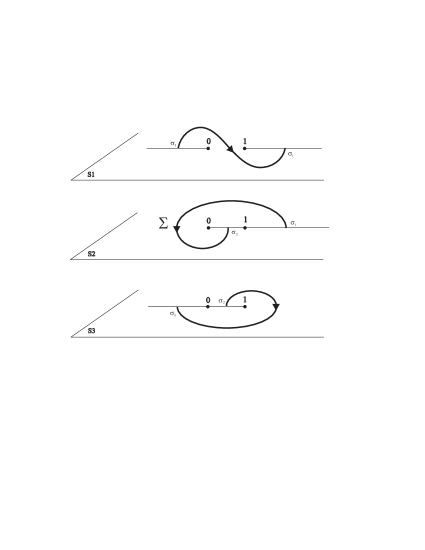
Figure 1: The contour $\Sigma$ on the appropriate Riemann surface for the function $t^{z-1}(1-t)^{w-1}$.

Now we prove our claim that (shifted) Jacobi polynomials with complex parameters are formal orthogonal polynomials.

Theorem 2.1

Let $\alpha,\beta,\alpha+\beta+1\in\mathbb{C}\setminus\{-1,-2,\ldots\}$, and consider the (complex) measure $\mu^{(\alpha,\beta)}$ defined by

$$\int h(x)\,d\mu^{(\alpha,\beta)}(x)=\lim_{z\to\alpha,w\to\beta}(1-e^{2\pi iz})^{-1}(1-e^{2\pi iw})^{-1}\int_{\Sigma}h(t)t^{z}(1-t)^{w}dt.$$

Then $\mu^{(\alpha,\beta)}$ forms a perfect system, with the corresponding $n$th formal orthogonal polynomial given by the (shifted) Jacobi polynomial $P_{n}^{(\alpha,\beta)}$.

• From (2.4) we obtain for the $k$th moment

  $$\int x^{k}\,d\mu^{(\alpha,\beta)}(x)=B(\alpha+1+k,\beta+1).$$

  The restrictions on the parameters $\alpha$ and $\beta$ guarantee that the determinant of the moment matrix,

  $$\det\Bigl{(}B(\alpha+r+s-1,\beta+1)\Bigr{)}_{1\leq r,s\leq n}=\prod_{i=1}^{n}\frac{\Gamma(\alpha+i)\Gamma(\beta+i)}{\Gamma(\alpha+\beta+n+i)}\prod_{1\leq r<s\leq n}(s-r),$$

  is different from zero. A proof for this formula uses Theorem 1 and 2 in [10, 11] (the moment matrix in the non-shifted case can be found in [25, 6.71.5]). Thus $\mu^{(\alpha,\beta)}$ forms a perfect system. Moreover, for $0\leq j\leq n-1$ we have according to (2.1) and (2.4)

  $$\int(1-x)^{j}P_{n}^{(\alpha,\beta)}(x)\,d\mu^{(\alpha,\beta)}(x)$$

  $$= \frac{(\alpha+1)_{n}}{n!}\sum_{k=0}^{n}\frac{(-n)_{k}(\alpha+\beta+n+1)_{k}}{(\alpha+1)_{k}k!}\ B(\alpha+k+1,\beta+j+1)$$

  $$= \frac{(-1)^{n}\Gamma(\alpha+n+1)\Gamma(\beta+j+1)}{\Gamma(\alpha+\beta+n+1)}\sum_{k=0}^{n}\frac{(-1)^{n-k}}{k!(n-k)!}\prod_{\ell=j+2}^{n}(\alpha+\beta+k+\ell).$$

  The sum on the right hand side is the divided difference $g_{j,n}[0,1,...,n]$ of the polynomial $g_{j,n}(x)=\prod_{l=j+2}^{n}(\alpha+\beta+x+l)$ of degree $n-j-1$. Since $n-j-1<n$, this is equal to $0$, which proves that the Jacobi polynomial is a formal orthogonal polynomial with respect to $\mu^{(\alpha,\beta)}$. $\Box$

2.2 Formal Wilson polynomials

In [27] J.A. Wilson introduced the (formal) Wilson polynomials

$$p_{n}(t^{2};a,b,c,d)=(a+b)_{n}(a+c)_{n}(a+d)_{n}\ \>{{}_{4}}F_{3}\left(\left.-n,a+b+c+d+n-1,a-t,a+t\atop a+b,a+c,a+d\right|1\right).$$ (2.5)

Due to Whipple’s identities [2, Theorem 3.3.3], one can show that these formal Wilson polynomials are symmetric in all four complex parameters $a,b,c,d$. Furthermore, with some conditions on these four parameters, the polynomials satisfy a complex orthogonality with respect to the Wilson weight function

$$w(t;a,b,c,d)=\frac{\Gamma(a+t)\Gamma(a-t)\Gamma(b+t)\Gamma(b-t)\Gamma(c+t)\Gamma(c-t)\Gamma(d+t)\Gamma(d-t)}{\Gamma(2t)\Gamma(-2t)}.$$

Suppose that

$$2a,a+b,a+c,a+d,2b,b+c,b+d,2c,c+d,2d\notin\{0,-1,-2,\ldots\},$$ (2.6)

so that the Wilson weight has only simple poles, and that

$$a+b+c+d\notin\{0,-1,-2,\ldots\}.$$ (2.7)

Furthermore denote by the contour ${\cal C}$ the imaginary axis deformed so as to separate the increasing sequences of poles ($\{a+k\}_{k=0}^{\infty},\{b+k\}_{k=0}^{\infty},\{c+k\}_{k=0}^{\infty},\{d+k\}_{k=0}^{\infty}$) from the decreasing ones ($\{-a-k\}_{k=0}^{\infty},\{-b-k\}_{k=0}^{\infty},\{-c-k\}_{k=0}^{\infty},\{-d-k\}_{k=0}^{\infty}$), and define the Wilson measure $\mu^{(a,b,c,d)}$ by

$$\int h(t)\,d\mu^{(a,b,c,d)}(t)=\int_{\mathcal{C}}h(t^{2})w(t;a,b,c,d)\,dt.$$ (2.8)

Wilson [27] shows the complex orthogonality relations

$$\int p_{m}(t;a,b,c,d)p_{n}(t;a,b,c,d)\,d\mu^{(a,b,c,d)}(t)=\delta_{mn}2iM_{n},$$

where

$$M_{n} = 2\pi n!\ (a+b+c+d+n-1)_{n}$$

$$\quad\times\frac{\Gamma(a+b+n)\Gamma(a+c+n)\Gamma(a+d+n)\Gamma(b+c+n)\Gamma(b+d+n)\Gamma(c+d+n)}{\Gamma(a+b+c+d+2n)}.$$

The perfectness of the singleton system $\mu^{(a,b,c,d)}$ follows from Lemma 3.4 below.

In some cases we obtain real orthogonality conditions with respect to positive measures on the real line [27]. If $\Re(a),\Re(b),\Re(c),\Re(d)>0$ and $a,b,c$ and $d$ are real except possibly for conjugate pairs, then $\cal C$ can be taken to be the imaginary axis and we obtain the real orthogonality

$$\int_{0}^{\infty}p_{m}(-x^{2};a,b,c,d)p_{n}(-x^{2};a,b,c,d)\left|\frac{\Gamma(a+ix)\Gamma(b+ix)\Gamma(c+ix)\Gamma(d+ix)}{\Gamma(2ix)}\right|^{2}dx=\delta_{mn}M_{n}.$$

Another case is when $a<0$ and $a+b,a+c,a+d$ are positive or a pair of complex conjugates occurs with positive real parts. We then get the same positive continuous weight function where some positive point masses are added. In these cases we obtain the Wilson polynomials $W_{n}(x^{2};a,b,c,d):=p_{n}(-x^{2};a,b,c,d)$ (see, e.g., [17]), which are real for real $x^{2}$.

Finally in the case that one of $a+b,a+c,a+d$ is equal to $-N+\epsilon$, with $N$ a nonnegative integer, we obtain a purely discrete orthogonality after dividing by $\Gamma(-N+\epsilon)$ and letting $\epsilon\to 0$. If we take the substitution $t\to x+a$ and the change of variables $\alpha=a+b-1,\beta=c+d-1,\gamma=a+d-1,\delta=a-d$ we then obtain the Racah polynomials

$$R_{n}(\lambda(x);\alpha,\beta,\gamma,\delta)=\>{{}_{4}}F_{3}\left(\left.-n,n+\alpha+\beta+1,-x,x+\gamma+\delta+1\atop\alpha+1,\beta+\delta+1,\gamma+1\right|1\right),$$

where $\lambda(x)=x(x+\gamma+\delta+1)$ and $\alpha+1=-N$ or $\beta+\delta+1=-N$ or $\gamma+1=-N$. They satisfy the discrete orthogonality

$$\sum_{x=0}^{N}\frac{(\alpha+1)_{x}(\gamma+1)_{x}(\beta+\delta+1)_{x}(\gamma+\delta+1)_{x}((\gamma+\delta+3)/2)_{x}}{(-\alpha+\gamma+\delta+1)_{x}(-\beta+\gamma+1)_{x}((\gamma+\delta+1)/2)_{x}(\delta+1)_{x}x!}\ R_{n}(\lambda(x);\alpha,\beta,\gamma,\delta)\>(\lambda(x))^{k}=0,$$

$k=0,\ldots,n-1$. Necessary and sufficient conditions for the positivity of the weights are quite messy. An example of sufficient conditions is given in [27, (3.5)].

The formal Wilson polynomials contain as limiting cases several families of orthogonal polynomials [27, Section 4][17, Chapter 2] like Hahn, dual Hahn, Meixner, Krawtchouk, Charlier, continuous Hahn, continuous dual Hahn, Meixner-Pollaczek, Jacobi, Laguerre and Hermite polynomials. Together they form the Askey scheme of hypergeometric orthogonal polynomials. Moreover, there exist $q$-analogues [17] for all these polynomials. The results of this paper should probably extend to this more general case.

2.3 Formal Wilson polynomials as a Jacobi transform

We now recall an integral relation between the Jacobi and the formal Wilson polynomials. We also give a short proof which will help us to find explicit expressions for the formal multiple Wilson polynomials in the next section.

Theorem 2.2 (T.H. Koornwinder)

Suppose that the conditions (2.6) and (2.7) hold, and that $\Re(c+d)>0$, $0<|\Re(t)|<\Re(a)$. Then we have

$$p_{n}(t^{2};a,b,c,d)=k_{n}\int_{0}^{1}P^{(\alpha,\beta)}_{n}(u)w^{(\alpha,\beta)}(u)K(u,t;a,b,c,d)\ du,$$ (2.9)

with $\alpha=a+b-1$ and $\beta=c+d-1$, the Jacobi weight function $w^{(\alpha,\beta)}(u)=u^{\alpha}(1-u)^{\beta}$, the constant $k_{n}=n!\ \Gamma(a+c+n)\Gamma(a+d+n)$ and the kernel (1.8).

Remark 2.3

T.H. Koornwinder already mentioned this Jacobi transform for the Wilson polynomials in [18, (3.3)]. In order to see that these formulas coincide, one has to make some parameter changes and substitute $1-\textrm{th}^{2}s\to u$. Notice also that (2.9) is a particular case of a formula due to Meijer [21, p.103].

• By comparing the explicit formulas (2.1) and (2.5) we see that it is sufficient to prove that, for $\ell\in\mathbb{N}$,

  $$\int_{0}^{1}u^{\ell}w^{(a-1,c+d-1)}(u)K(u,t;a,0,c,d)\>du=\frac{(a-t)_{\ell}(a+t)_{\ell}}{\Gamma(a+c+\ell)\Gamma(a+d+\ell)}.$$ (2.10)

  By definition of the kernel (1.8) we have

  $$K(u,t;a,0,c,d)=(a-t)_{\ell}(a+t)_{\ell}\ K(u,t;a+\ell,0,c,d),$$

  and $u^{\ell}w^{(a-1,c+d-1)}(u)=w^{(a+\ell-1,c+d-1)}(u)$. Furthermore, Euler’s formula gives the symmetry $K(u,-t;a+\ell,0,c,d)=K(u,t;a+\ell,0,c,d)$. By replacing $a+\ell$ by $a$ and possibly $t$ by $-t$, we see that it remains to prove that, for $0<\Re(t)<\Re(a)$ and $\Re(c+d)>0$,

  $$\int_{0}^{1}w^{(a-1,c+d-1)}(u)K(u,t;a,0,c,d)\>du=\frac{1}{\Gamma(a+c)\Gamma(a+d)}.$$ (2.11)

  Denoting the left hand side of (2.11) by $J$, we have by definition of the kernel

  $$J=\frac{1}{\Gamma(a-t)\Gamma(a+t)\Gamma(c+d)}\int_{0}^{1}w^{(a-t-1,c+d-1)}(u)\>{{}_{2}}F_{1}\left(\left.c-t,d-t\atop c+d\right|1-u\right)du.$$

  In order to exchange the order of summation and integration, we notice that, if $\Re(C-A-B)>0$,

  $$\lim_{y\to 1-}\ \max_{v\in[0,1]}\left|\>{{}_{2}}F_{1}\left(\left.A,B\atop C\right|yv\right)-\>{{}_{2}}F_{1}\left(\left.A,B\atop C\right|v\right)\right|=0,$$

  which follows by observing that $\frac{\Gamma(A+k)\Gamma(B+k)}{\Gamma(C+k)\Gamma(1+k)}=k^{A+B-C-1}(1+\mathcal{O}(k^{-1}))$, _k→∞, by Stirling’s formula. Consequently, using the assumptions $\Re(2t)>0$, $\Re(a-t)>0$, $\Re(c+d)>0$ together with (2.3) we obtain by uniform convergence

  $$J = \frac{1}{\Gamma(a-t)\Gamma(a+t)\Gamma(c+d)}\lim_{y\to 1-}\int_{0}^{1}w^{(a-t-1,c+d-1)}(u)\>{{}_{2}}F_{1}\left(\left.c-t,d-t\atop c+d\right|y(1-u)\right)du$$

  $$= \lim_{y\to 1-}\sum_{k=0}^{\infty}\frac{(c-t)_{k}(d-t)_{k}\ y^{k}}{\Gamma(a-t)\Gamma(a+t)\Gamma(c+d+k)k!}\int_{0}^{1}w^{(a-t-1,c+d+k-1)}(u)\>du$$

  $$= \lim_{y\to 1-}\frac{1}{\Gamma(a+t)\Gamma(a+c+d-t)}\>{{}_{2}}F_{1}\left(\left.c-t,d-t\atop a+c+d-t\right|y\right).$$

  By assumption on the parameters, $\Re(a+c+d-t-(c-t+d-t))>0$, and hence we get from the Gauss formula [2, Theorem 2.2.2],[1, 15.1.20]

  $$J=\frac{1}{\Gamma(a+t)\Gamma(a+c+d-t)}\>{{}_{2}}F_{1}\left(\left.c-t,d-t\atop a+c+d-t\right|1\right)=\frac{1}{\Gamma(a+d)\Gamma(a+c)},$$

  as claimed in (2.11). $\Box$

3 Multiple Wilson as a Jacobi-Piñeiro transform

3.1 Jacobi-Piñeiro with complex parameters

The Jacobi-Piñeiro polynomials are defined by a Rodrigues formula

$$P_{\vec{n}}^{(\vec{\alpha},\beta)}(t)=\frac{1}{\vec{n}!}(1-t)^{-\beta}\prod_{j=1}^{m}\left(t^{-\alpha_{j}}\frac{d^{n_{j}}}{dt^{n_{j}}}t^{n_{j}+\alpha_{j}}\right)(1-t)^{|\vec{n}|+\beta},$$ (3.1)

where $\vec{n}!=\prod_{j=1}^{m}n_{j}!$. It is well known [23] that, provided that $\alpha_{j}>-1,\beta>-1$ and $\alpha_{\ell}-\alpha_{k}\not\in\mathbb{Z}$ for $\ell\neq k$, the Jacobi-Piñeiro polynomials are orthogonal with respect to the (positive) Jacobi weights $w^{(\alpha_{j},\beta)}$, $j=1,\ldots,m$, on the interval $[0,1]$. Notice that these weights form an AT system, and hence we obtain a perfect system of measures. Similar to Theorem 2.1, we show below that for complex parameters we keep formal multiple orthogonal polynomials of type II. Here we use the measures $\mu^{(\alpha_{j},\beta)}$ of Theorem 2.1 which have as support the contour $\Sigma$, but can be reduced to complex Jacobi weights $w^{(\alpha_{j},\beta)}$ on the interval $[0,1]$ in the case $\Re(\alpha_{j})>-1,\Re(\beta)>-1$.

Theorem 3.1

Let $\alpha_{j},\beta,\alpha_{j}+\beta\in\mathbb{C}\setminus\{-1,-2,...\}$. Then the measures $\mu^{(\alpha_{j},\beta)}$, $j=1,...,m$, of Theorem 2.1 form a perfect system. The corresponding formal multiple orthogonal polynomial of type II with respect to the multi-index $\vec{n}$ is given by (3.1).

• From Theorem 1 and 2 in [10, 11] we obtain for the determinant of the matrix of moments (1.5) the expression

  $$D_{\vec{n}}^{\vec{\alpha},\beta} = \left(\prod_{i=1}^{|\vec{n}|}\Gamma(\beta+i)\right)\left(\prod_{j=1}^{m}\prod_{i=1}^{n_{j}}\frac{\Gamma(\alpha_{j}+i)}{\Gamma(\alpha_{j}+\beta+\vec{n}+i)}\right)$$

  $$\qquad\times\left(\prod_{j=1}^{m}\prod_{1\leq r<s\leq n_{j}}(s-r)\right)\left(\prod_{1\leq i<j\leq m}\prod_{s=1}^{n_{i}}\prod_{r=1}^{n_{j}}(\alpha_{j}-\alpha_{i}+r-s\right).$$

  For our choice of parameters, this expression is different from zero, and hence every multi-index is normal.

  Our claim on the (formal) orthogonality of Jacobi-Piñeiro polynomials will be shown by induction on $m$. For $m=1$, equation (3.1) reduces to (2.1), and the claim follows from Theorem 2.1. For $m>1$, we observe first that, by the Rodrigues formula (3.1),

  $$P_{\vec{n}}^{(\vec{\alpha},\beta)}(t)=\frac{t^{-\alpha_{1}}(1-t)^{-\beta}}{n_{1}!}\frac{d^{n_{1}}}{dt^{n_{1}}}\left(t^{\alpha_{1}+n_{1}}(1-t)^{\beta+n_{1}}P_{(n_{2},...,n_{m})}^{((\alpha_{2},...,\alpha_{m}),\beta+n_{1})}(t)\right).$$ (3.2)

  By induction hypothesis, $P_{(n_{2},...,n_{m})}^{((\alpha_{2},...,\alpha_{m}),\beta+n_{1})}$ is a polynomial of degree $|\vec{n}|-n_{1}$, and thus there exist scalars $c_{j}$ with

  $$P_{(n_{2},...,n_{m})}^{((\alpha_{2},...,\alpha_{m}),\beta+n_{1})}(t)=\sum_{j=0}^{|\vec{n}|-n_{1}}c_{j}P^{(\alpha_{1}+n_{1},\beta+n_{1})}_{j}(t).$$

  From the Rodrigues formula for $m=1$ and (3.2) we conclude that

  $$P_{\vec{n}}^{(\vec{\alpha},\beta)}(t)=\sum_{j=0}^{|\vec{n}|-n_{1}}c_{j}P^{(\alpha_{1},\beta)}_{j+n_{1}}(t),$$

  implying that $P_{\vec{n}}^{(\vec{\alpha},\beta)}$ is a polynomial of degree $|\vec{n}|$ with $\int t^{k}P_{\vec{n}}^{(\vec{\alpha},\beta)}(t)\,d\mu^{(\alpha_{1},\beta)}=0$ for $k=0,1,...,n_{1}-1$ by Theorem 2.1. The other orthogonality conditions are obtained by observing that (3.1) remains invariant if one changes the order in the product in (3.1). $\Box$

With help of the Leibniz rule applied to the Rodrigues formula, the authors in [14] derive for $m=2$ an explicit expression in terms of $m=2$ sums. We now give a generalization of this formula for $m\geq 2$, using the notation

$$\>\mathcal{M}_{q,\vec{n}}^{p;r}\left(\left.\vec{f};\vec{g}_{1}:\cdots:\vec{g}_{r}\atop\vec{\phi};\vec{\psi}_{1}:\cdots:\vec{\psi}_{r}\right|\vec{x}\right)$$

$$:= \underbrace{\sum_{k_{1}=0}^{n_{1}}\cdots\sum_{k_{m}=0}^{n_{m}}}_{\mbox{$m$ sums}}\frac{\prod\limits_{\ell=1}^{p}(f_{\ell})_{|\vec{k}|}}{\prod\limits_{\ell=1}^{q}(\phi_{\ell})_{|\vec{k}|}}\frac{\prod\limits_{i=1}^{r}(g_{i,1})_{|\vec{k}|-k_{1}}\cdots(g_{i,m-1})_{k_{m}}}{\prod\limits_{i=1}^{r}(\psi_{i,1})_{|\vec{k}|-k_{1}}\cdots(\psi_{i,m-1})_{k_{m}}}\prod_{j=1}^{m}(-n_{j})_{k_{j}}\frac{x_{j}^{k_{j}}}{k_{j}!},$$

where $\vec{k}=(k_{1},\ldots,k_{m})$, $\vec{n}\in\left(\mathbb{N}\cup\{0\}\right)^{m}$, $\vec{f}\in\mathbb{C}^{p}$, $\vec{\phi}\in\mathbb{C}^{q}$ and $\vec{g}_{1},\ldots,\vec{g}_{r},\vec{\psi}_{1},\ldots,\vec{\psi}_{r}\in\mathbb{C}^{m-1}$. We also give in (3.5) another new explicit expression for the formal Jacobi-Piñeiro polynomials which reduces to (2.2) if $m=1$.

Theorem 3.2

Let $\vec{e}=(1,\ldots,1)$ be a multi-index of length $m$ and $s(\vec{n})=(n_{1},n_{1}+n_{2},\ldots,|\vec{n}|)$. Denote by $\vec{v}^{(j)}$ the vector $\vec{v}$ without the $j$th component. For the Jacobi-Piñeiro polynomials we have the hypergeometric representations

$$P_{\vec{n}}^{(\vec{\alpha},\beta)}(t)=\frac{(\vec{\alpha}+\vec{e})_{\vec{n}}}{\vec{n}!}\>\mathcal{M}_{1,\vec{n}}^{1;2}\left(\left.(\alpha_{1}+\beta+n_{1}+1);(\vec{\alpha}+\vec{n}+\vec{e})^{(m)}:(\vec{\alpha}+s(\vec{n})+(\beta+1)\vec{e})^{(1)}\atop(\alpha_{1}+1);(\vec{\alpha}+\vec{e})^{(1)}:(\vec{\alpha}+s(\vec{n})+(\beta+1)\vec{e})^{(m)}\right|t\vec{e}\right)$$ (3.4)

and

$$P_{\vec{n}}^{(\vec{\alpha},\beta)}(t)=\frac{(\vec{\alpha}+\vec{e})_{\vec{n}}}{\vec{n}!}\ (1-t)^{-\beta}\>{{}_{m+1}}F_{m}\left(\left.\vec{\alpha}+\vec{n}+\vec{e},-\beta-|\vec{n}|\atop\vec{\alpha}+\vec{e}\right|t\right),$$ (3.5)

where $\vec{n}!=\prod_{j=1}^{m}n_{j}!$ and $(\vec{\alpha}+\vec{e})_{\vec{n}}=\prod_{j=1}^{m}(\alpha_{j}+1)_{n_{j}}$.

• We prove (3.4) and (3.5) by induction on $m$. For $m=1$, equations (3.4) and (3.5) reduce to (2.1) and (2.2), respectively.

  In case $m\geq 2$, we use formula (3.2), where the induction hypothesis enables us to express the right hand polynomial $P_{\vec{n}^{(1)}}^{(\vec{\alpha}^{(1)},\beta+n_{1})}$ as a hypergeometric sum. After exchanging the order of summation and differentiation (for $|t|<1$ in case of formula (3.5)), we apply the formulas

  $$t^{-\alpha_{1}}(1-t)^{-\beta}\frac{d^{n_{1}}}{dt^{n_{1}}}\left(t^{\alpha_{1}+n_{1}+|\vec{k}^{(1)}|}(1-t)^{\beta+n_{1}}\right)$$

  $$= (\alpha_{1}+1)_{n_{1}}\sum_{k_{1}=0}^{n_{1}}\frac{(\alpha_{1}+\beta+n_{1}+1)_{|\vec{k}|}}{(\alpha_{1}+1)_{|\vec{k}|}}\frac{(\alpha_{1}+n_{1}+1)_{|\vec{k}|-k_{1}}}{(\alpha_{1}+\beta+n_{1}+1)_{|\vec{k}|-k_{1}}}\frac{(-n_{1})_{k_{1}}t^{|\vec{k}|}}{k_{1}!}$$

  and

  $$t^{-\alpha_{1}}\frac{d^{n_{1}}}{dt^{n_{1}}}t^{\alpha_{1}+n_{1}+i}=\frac{(\alpha_{1}+1)_{n_{1}}(\alpha_{1}+n_{1}+1)_{i}}{(\alpha_{1}+1)_{i}}\ t^{i},$$ (3.7)

  and obtain the right-hand expressions of (3.4), and (3.5), respectively. It remains to prove the claims (Proof. ) and (3.7), the second one being obvious. We observe that the left-hand side of (Proof. ) can be transformed using the Rodrigues formula for $m=1$ and (2.1), leading to the expression

  $$t^{|\vec{k}^{(1)}|}(\alpha_{1}+|\vec{k}^{(1)}|+1)_{n_{1}}\>{{}_{2}}F_{1}\left(\left.-n_{1},\alpha_{1}+|\vec{k}^{(1)}|+\beta+n_{1}+1\atop\alpha_{1}+|\vec{k}^{(1)}|+1\right|t\right)$$

  $$= (\alpha_{1}+|\vec{k}^{(1)}|+1)_{n_{1}}\sum_{k_{1}=0}^{n_{1}}\frac{(-n_{1})_{k_{1}}(\alpha_{1}+|\vec{k}^{(1)}|+\beta+n_{1}+1)_{k_{1}}}{(\alpha_{1}+|\vec{k}^{(1)}|+1)_{k_{1}}}\frac{t^{|\vec{k}|}}{k_{1}!}$$

  $$= (\alpha_{1}+1)_{n_{1}}\sum_{k_{1}=0}^{n_{1}}\frac{(\alpha_{1}+\beta+n_{1}+1)_{|\vec{k}|}}{(\alpha_{1}+1)_{|\vec{k}|}}\frac{(\alpha_{1}+n_{1}+1)_{|\vec{k}|-k_{1}}}{(\alpha_{1}+\beta+n_{1}+1)_{|\vec{k}|-k_{1}}}\frac{(-n_{1})_{k_{1}}t^{|\vec{k}|}}{k_{1}!},$$

  as claimed in (Proof. ). $\Box$

In the above proof we have shown implicitly that the right hand side of (3.5) is a polynomial of degree $\leq|\vec{n}|$ in $t$.

With the explicit formula (3.4) it is possible to compute the recurrence coefficients by comparing the highest coefficients in the recurrence relation of order $m+1$, see [14] for $m=2$. The resulting formulas are quite complicated, and thus we omit further details.

3.2 Formal multiple Wilson polynomials

We now consider $m$ Wilson weights

$$w(\cdot;a,b_{j},c,d),\quad j=1,\ldots,m,\quad\mbox{$b_{\ell}-b_{k}\not\in\mathbb{Z}$,\quad$\ell\neq k$},$$ (3.8)

defined as in (1.6), that is, we change only one parameter (recall the symmetry of the Wilson weights in all four parameters). Similar as in the scalar case (Wilson polynomials) we suppose that for $j=1,\ldots,m$

$$2a,a+b_{j},a+c,a+d,2b_{j},b_{j}+c,b_{j}+d,2c,c+d,2d\notin\{0,-1,-2,\ldots\},$$ (3.9)

so that the $m$ Wilson weights have only simple poles, and that

$$a+b_{j}+c+d\notin\{0,-1,-2,\ldots\}.$$ (3.10)

As in the scalar case, we write $\mu^{(a,b_{j},c,d)}$ for the resulting measures, where it is possible to choose a joint contour ${\cal C}$ which is the imaginary axis deformed so as to separate the increasing sequences of poles ($\{a+k\}_{k=0}^{\infty},\{b_{1}+k\}_{k=0}^{\infty},\ldots,\{b_{m}+k\}_{k=0}^{\infty},\{c+k\}_{k=0}^{\infty},\{d+k\}_{k=0}^{\infty}$) from the decreasing ones ($\{-a-k\}_{k=0}^{\infty},\{-b_{1}-k\}_{k=0}^{\infty},\ldots,\{-b_{m}-k\}_{k=0}^{\infty},\{-c-k\}_{k=0}^{\infty},\{-d-k\}_{k=0}^{\infty}$).

Let us show that the (possibly complex) Wilson measures $\mu^{(a,b_{j},c,d)}$ form a perfect system. The corresponding multiple orthogonal polynomials will then be referred to as formal multiple Wilson polynomials. A basic observation in what follows is that, under some additional conditions, the formal multiple Wilson polynomials can be written as a Jacobi-Piñeiro transform, similar to (2.9).

Theorem 3.3

Suppose that (3.9) and (3.10) hold and that $b_{\ell}-b_{k}\not\in\mathbb{Z}$, $\ell\neq k$. Then the Wilson measures $\mu^{(a,b_{j},c,d)}$ for $j=1,\ldots,m$ form a perfect system.

If $\Re(a)>0$ and $\Re(c+d)>0$, the formal multiple Wilson polynomial with multi-index $\vec{n}$ can be written as

$$p_{\vec{n}}(t^{2};a,\vec{b},c,d)=k_{\vec{n}}\int_{0}^{1}P^{(\vec{\alpha},\beta)}_{\vec{n}}(u)w^{(a-1,\beta)}(u)K(u,t;a,0,c,d)\>du,$$ (3.11)

for $0<|\Re(t)|<\Re(a)$, where $\vec{\alpha}=(a+b_{1}-1,\ldots,a+b_{m}-1)=(a-1)\vec{e}+\vec{b}$ and $\beta=c+d-1$. The normalizing constant $k_{\vec{n}}=\vec{n}!\ \Gamma(a+c+|\vec{n}|)\Gamma(a+d+|\vec{n}|)$ is chosen so that it corresponds with (2.9) in the case $m=1$ and the kernel $K(u,t;a,b,c,d)$ is defined as in (1.8).

Before we prove this theorem we need some technical lemmas.

Lemma 3.4

The system of $m$ measures $\mu_{1},\ldots,\mu_{m}$ is perfect if and only if, for every multi-index $\vec{n}$, there exists a polynomial $p_{\vec{n}}$ of exactly degree $|\vec{n}|$ so that

$$\int p_{\vec{n}}(z)z^{k}\>d\mu_{j}(z)=0,\qquad k=0,\ldots,n_{j}-1,\quad j=1,\ldots,m,$$ (3.12)

and

$$\int p_{\vec{n}}(z)z^{n_{j}}\>d\mu_{j}(z)\not=0,\qquad j=1,\ldots,m.$$ (3.13)

In this case, $p_{\vec{n}}$ is the (up to normalization unique) multiple orthogonal polynomial of type II with respect to $\vec{n}$.

• Suppose first that $\mu_{1},...,\mu_{m}$ is perfect, and take as $p_{\vec{n}}$ the multiple orthogonal polynomial of type II with respect to $\vec{n}$. Then it only remains to verify (3.13). Suppose the contrary, that is, $\int p_{\vec{n}}(z)z^{n_{j}}\>d\mu_{j}(z)=0$ for some $j$. Then $p_{\vec{n}}$ is also a multiple orthogonal polynomial of type II with respect to $\vec{\nu}=(n_{1},...,n_{j-1},n_{j}+1,n_{j+1},...,n_{m})$, in contrast to the normality of the multi-index $\vec{\nu}$.

  We will prove the other implication of this lemma by showing by induction on the length $|\vec{n}|$ that $\vec{n}$ is normal. The multi-index $\vec{0}$ is always normal, suppose therefore that $\vec{n}$ is of length $\geq 1$, with its $j$th component strictly greater than $0$. Let $q_{\vec{n}}$ be a multiple orthogonal polynomial for $\vec{n}$. If $q_{\vec{n}}$ would have degree strictly less than $|\vec{n}|$, then it would be a multiple orthogonal polynomial for the multi-index $\vec{\nu}=(n_{1},...,n_{j-1},n_{j}-1,n_{j+1},...,n_{m})$ with length $|\vec{n}|-1$. By normality of $\vec{\nu}$ we then have that there exists a nonzero constant $c$ so that $q_{\vec{n}}=cp_{\vec{\nu}}$. Thus $\int q_{\vec{n}}(z)z^{n_{j}-1}\>d\mu_{j}(z)\not=0$ by (3.13), in contradiction to the orthogonality relation (3.12) for $q_{\vec{n}}$. As a consequence, $q_{\vec{n}}$ has the precise degree $|\vec{n}|$, and thus $\vec{n}$ is normal. $\Box$

Lemma 3.5

Suppose that the singleton systems $\mu_{j}$ form a perfect system for $j=1,...,m$, with corresponding orthogonal polynomials $\{p_{n}^{(j)}\}_{n}$. Then the system of $m$ measures $\mu_{1},\ldots,\mu_{m}$ is perfect if and only if, for every multi-index $\vec{n}$, there exists a polynomial $p_{\vec{n}}$ and scalars $c_{\vec{n},k}^{(j)}$ so that

$$p_{\vec{n}}(x)=\sum_{\ell=n_{j}}^{|\vec{n}|}c_{\vec{n},\ell}^{(j)}p_{\ell}^{(j)}(x),\qquad c_{\vec{n},n_{j}}^{(j)}\neq 0,\qquad c_{\vec{n},|\vec{n}|}^{(j)}\neq 0,\qquad j=1,\ldots,m.$$ (3.14)

In this case, $p_{\vec{n}}$ is the (up to normalization unique) multiple orthogonal polynomial of type II with respect to $\vec{n}$.

• If $\vec{n}$ is normal and $p_{\vec{n}}$ is the corresponding multiple orthogonal polynomial, then (3.14) follows by taking

  $$c_{\vec{n},\ell}^{(j)}=\frac{\int p_{\vec{n}}(x)p_{\ell}^{(j)}(x)d\mu_{j}(x)}{\int\left(p_{\ell}^{(j)}(x)\right)^{2}d\mu_{j}(x)},$$ (3.15)

  where we observe that the denominator is nontrivial according to (3.12),(3.13) for the singleton system $\mu_{j}$. In addition, $c_{\vec{n},\ell}^{(j)}=0$ for $\ell<n_{j}$ by (3.12), $c_{\vec{n},n_{j}}^{(j)}\neq 0$ by (3.13), and $c_{\vec{n},|\vec{n}|}^{(j)}\neq 0$.

  Conversely, (3.14) plus the perfectness of the singleton system $\mu_{j}$ implies (3.12),(3.13), and hence the system $\mu_{1},\ldots,\mu_{m}$ is perfect by Lemma 3.4. $\Box$

We now prove Theorem 3.3 by showing that (the analytic extension of) the integral expression (3.11) is a possible candidate for a formal multiple Wilson polynomial.

• According to the assumptions (3.9) and (3.10) of Theorem 3.3, we find that $\alpha_{j},\beta,\alpha_{j}+\beta+1\in\mathbb{C}\setminus\{-1,-2,\ldots\}$, $j=1,\ldots,m$, and $\alpha_{\ell}-\alpha_{k}\not\in\mathbb{Z}$ whenever $\ell\neq k$. It follows from Theorem 3.1 that the Jacobi-Piñeiro system $\mu^{(\alpha_{j},\beta)}$, $j=1,...,m$, is perfect. From Lemma 3.5 we may conclude that there exists scalars $c_{\vec{n},k}^{(j)}$ so that

  $$P^{(\vec{\alpha},\beta)}_{\vec{n}}(t)=\sum_{\ell=n_{j}}^{|\vec{n}|}c_{\vec{n},\ell}^{(j)}P^{(\alpha_{j},\beta)}_{\ell}(t),\qquad c_{\vec{n},n_{j}}^{(j)}\neq 0,\qquad c_{\vec{n},|\vec{n}|}^{(j)}\neq 0,j=1,\ldots,m.$$

  From, e.g., (3.4) we see that Jacobi-Piñeiro polynomials are rational functions in each of the parameters $\alpha_{j}$ or $\beta$. Taking into account (2.4) and (3.15), we may conclude that any of the coefficients $c_{\vec{n},\ell}^{(j)}$ is a meromorphic function in each of the parameters $\alpha_{j}$ or $\beta$. We now introduce

  $$q_{\vec{n}}(t^{2};a,\vec{b},c,d) = k_{\vec{n}}\int_{0}^{1}P^{(\vec{\alpha},\beta)}_{\vec{n}}(u)w^{(a-1,\beta)}(u)K(u,t;a,0,c,d)\>du.$$

  This function is well defined for $0<|\Re(t)|<\Re(a)$ if $\Re(a)>0$ and $\Re(c+d)>0$. However, using (2.9), we obtain for every $j=1,\ldots,m$ that

  $$q_{\vec{n}}(t^{2};a,\vec{b},c,d) = k_{\vec{n}}\sum_{\ell=n_{j}}^{|\vec{n}|}c_{\vec{n},\ell}^{(j)}\int_{0}^{1}P^{(\alpha_{j},\beta)}_{\ell}(x)w^{(\alpha_{j},\beta)}(u)K(u,t;a,b_{j},c,d)\>du,$$

  $$= \sum_{\ell=n_{j}}^{|\vec{n}|}\frac{\vec{n}!}{\ell!}\frac{\Gamma(a+c+|\vec{n}|)\Gamma(a+d+|\vec{n}|)}{\Gamma(a+c+\ell)\Gamma(a+d+\ell)}\ c_{\vec{n},\ell}^{(j)}\ p_{\ell}(t^{2};a,b_{j},c,d),$$

  and thus

  $$q_{\vec{n}}(t^{2};a,\vec{b},c,d) = \sum_{\ell=n_{j}}^{|\vec{n}|}\frac{\vec{n}!}{\ell!}(a+c+\ell)_{|\vec{n}|-\ell}\>(a+d+\ell)_{|\vec{n}|-\ell}\ c_{\vec{n},\ell}^{(j)}\ p_{\ell}(t^{2};a,b_{j},c,d)$$ (3.16)

  $$= \sum_{\ell=n_{j}}^{|\vec{n}|}d_{\vec{n},\ell}^{(j)}\ p_{\ell}(t^{2};a,b_{j},c,d).$$

  Observing that the expressions on the right-hand side of (3.16) are polynomials in $t$ and meromorphic in any of the parameters $a,\vec{b},c,d$, we see that the right hand expression of (3.16) is well defined and independent of $j$ for any choice of $t$ and of the parameters $a,\vec{b},c,d$, as long as (3.9) and (3.10) hold and $b_{\ell}-b_{k}\not\in\mathbb{Z}$, $\ell\neq k$. Moreover, the new coefficients $d_{\vec{n},n_{j}}^{(j)}$ and for $d_{\vec{n},|\vec{n}|}^{(j)}$ are different from zero.

  Thus, $q_{\vec{n}}(t^{2};a,\vec{b},c,d)$ defined by (3.16) is a suitable candidate for a formal multiple Wilson polynomial, and the system of Wilson measures is perfect by Lemma 3.5. $\Box$

We now want to deduce explicit expressions for the formal multiple Wilson polynomials based on the explicit expressions (3.4) and (3.5) for the Jacobi-Piñeiro polynomials. Here we use the Kampé de Fériet series [24]

$$\>F_{q:q_{1};q_{2}}^{p:p_{1};p_{2}}\left(\left.\vec{f}:\vec{g};\vec{h}\atop\vec{\phi}:\vec{\psi};\vec{\xi}\right|x,y\right):=\sum_{k=0}^{\infty}\frac{\prod\limits_{\ell=1}^{p}(f_{\ell})_{k}}{\prod\limits_{\ell=1}^{q}(\phi_{\ell})_{k}}\sum_{j=0}^{k}\frac{\prod\limits_{\ell=1}^{p_{1}}(g_{\ell})_{k-j}\prod\limits_{\ell=1}^{p_{2}}(h_{\ell})_{j}}{\prod\limits_{\ell=1}^{q_{1}}(\psi_{\ell})_{k-j}\prod\limits_{\ell=1}^{q_{2}}(\xi_{\ell})_{j}}\frac{x^{k-j}}{(k-j)!}\frac{y^{j}}{j!},$$ (3.17)

which are a generalization of the 4 Appell series in 2 variables. Notice that, for $p=q=0$, the Kampé de Fériet series is a product of two hypergeometric series. Also, in the case $m=2$, our functions $\mathcal{M}_{q,\vec{n}}^{p;r}$ defined in (3.1) are (finite) Kampé de Fériet series

$$\>\mathcal{M}_{q,(n_{1},n_{2})}^{p;r}\left(\left.\vec{f};g_{1}:\cdots:g_{r}\atop\vec{\phi};\psi_{1}:\cdots:\psi_{r}\right|(x_{1},x_{2})\right)=\>F_{q:0;r}^{p:1;r+1}\left(\left.\vec{f}:(-n_{1});(-n_{2},g_{1},...,g_{r})\atop\vec{\phi}:();(\psi_{1},...,\psi_{r})\right|x_{1},x_{2}\right).$$ (3.18)

In what follows the parameters in the Kampé de Fériet series will always be chosen so that the sum in (3.17) is finite, and hence we are not concerned with convergence problems.

Corollary 3.6

Let $\vec{e}=(1,\ldots,1)$ be a multi-index of length $m$, $s(\vec{n})=(n_{1},n_{1}+n_{2},\ldots,|\vec{n}|)$ and $\sigma_{j}=a+b_{j}+c+d-1$, $j=1,\ldots,m$. Denote by $\vec{v}^{(j)}$ the vector $\vec{v}$ without the $j$th component. For the multiple Wilson polynomials we have the hypergeometric representations

$$p_{\vec{n}}(t^{2};a,\vec{b},c,d)=(a\vec{e}+\vec{b})_{\vec{n}}(a+c)_{|\vec{n}|}(a+d)_{|\vec{n}|}$$ (3.19)

$$\qquad\qquad\times\>\mathcal{M}_{3,\vec{n}}^{3;2}\left(\left.(a-t,a+t,\sigma_{1}+n_{1});(a\vec{e}+\vec{b}+\vec{n})^{(m)}:(\vec{\sigma}+s(\vec{n}))^{(1)}\atop(a+c,a+d,a+b_{1});(a\vec{e}+\vec{b})^{(1)}:(\vec{\sigma}+s(\vec{n}))^{(m)}\right|\vec{e}\right)$$

and

$$p_{\vec{n}}(t^{2};a,\vec{b},c,d)=(a\vec{e}+\vec{b})_{\vec{n}}(a+c)_{|\vec{n}|}(a+d)_{|\vec{n}|}$$ (3.20)

$$\qquad\qquad\times\>F_{2:0;m}^{2:1;m+1}\left(\left.(a-t,a+t):(c+d-1);(a\vec{e}+\vec{b}+\vec{n},1-c-d-|\vec{n}|)\atop(a+c,a+d):();(a\vec{e}+\vec{b})\right|1,1\right)$$

where $(a\vec{e}+\vec{b})_{\vec{n}}=\prod_{j=1}^{m}(a+b_{j})_{n_{j}}$.

• First note that $(1-x)^{-\beta}=\sum_{\ell=0}^{\infty}(\beta)_{l}\frac{x^{\ell}}{\ell!}$, which converges in the unit disk, so that the expression (3.5) can then be written as

  $$P_{\vec{n}}^{(\vec{\alpha},\beta)}(t)=\frac{(\vec{\alpha}+\vec{e})_{\vec{n}}}{\vec{n}!}\>F_{0:0;m}^{0:1;m+1}\left(\left.-:(\beta);(\vec{\alpha}+\vec{n}+\vec{e},-\beta-|\vec{n}|)\atop-:-;(\vec{\alpha}+\vec{e})\right|t,t\right).$$ (3.21)

  Then start from the Jacobi-Piñeiro transform (3.11) and replace the Jacobi-Piñeiro polynomial $P_{\vec{n}}^{(\vec{\alpha},\beta)}$ by its explicit expressions (3.4) and (3.21), respectively. Since the sums are finite, we can interchange the integral with the sums. Applying (2.10) then completes the proof. $\Box$

For $m=2$, we may apply (3.18) to (3.19), leading to a representation as a Kampé de Fériet series of type $F_{3:0;2}^{3:1;3}$. It seems to be non-trivial to derive from this formula the representation (3.20) as a Kampé de Fériet series of type $F_{2:0;2}^{2:1;3}$.

4 Limit relations

In this section we consider some cases in which the orthogonality conditions of the formal multiple Wilson polynomials reduce to orthogonality conditions with respect to a positive measure on the real line. We then recover the multiple Wilson and multiple Racah polynomials. Next we use the limit relations between the orthogonal polynomials in the Askey table [17] to obtain some new examples of multiple orthogonal polynomials and some known examples. In particular we look at what happens with the explicit expressions (3.19) and (3.20) applying these limit relations. Most of these examples are known to be AT systems (which implies that every multi-index is normal).

4.1 Multiple Wilson

With some restrictions on the parameters the orthogonality conditions of the formal multiple Wilson polynomials reduce to real orthogonality conditions with respect to positive measures on the real line. Let $b_{j}>0$, $j=1,\ldots,m$, $b_{\ell}-b_{k}\not\in\mathbb{Z}$ whenever $\ell\neq k$, $\Re(a),\Re(c),\Re(d)>0$ and $a,c,d$ be real except for a conjugate pair. In that case the imaginary axis can be taken as the contour $\cal C$. The multiple Wilson polynomials

$$W_{\vec{n}}(x^{2};a,\vec{b},c,d):=p_{\vec{n}}(-x^{2};a,\vec{b},c,d)$$ (4.1)

then satisfy the real orthogonality relations

$$\int_{0}^{\infty}(x^{2})^{k}\>W_{\vec{n}}(x^{2};a,\vec{b},c,d)\left|\frac{\Gamma(a+ix)\Gamma(b_{j}+ix)\Gamma(c+ix)\Gamma(d+ix)}{\Gamma(2ix)}\right|^{2}dx=0,$$

$k=0,\ldots,n_{j}-1$, $j=1,\ldots,m$. If $a<0$, $a+b_{j}>0$, $j=1,\ldots,m$, and $a+c,a+d$ are positive or a pair of complex conjugates with positive real parts, then we obtain the same orthogonality conditions but with some extra positive point masses.

4.2 Multiple Racah

As in the scalar case it is also possible to obtain a purely discrete orthogonality. The multiple Racah polynomials $R_{\vec{n}}(\cdot;\vec{\alpha},\beta,\gamma,\delta)$ (where we only change the parameter $\alpha$ with $\alpha_{\ell}-\alpha_{k}\not\in\mathbb{Z}$ whenever $\ell\neq k$) satisfy the discrete orthogonality

$$\sum_{x=0}^{N}\frac{(\alpha_{j}+1)_{x}(\gamma+1)_{x}(\beta+\delta+1)_{x}(\gamma+\delta+1)_{x}((\gamma+\delta+3)/2)_{x}}{(-\alpha_{j}+\gamma+\delta+1)_{x}(-\beta+\gamma+1)_{x}((\gamma+\delta+1)/2)_{x}(\delta+1)_{x}x!}\ R_{\vec{n}}(\lambda(x);\vec{\alpha},\beta,\gamma,\delta)\>(\lambda(x))^{k}=0,$$

$k=0,\ldots,n-1$, $j=1,\ldots,m$, where

$$\lambda(x)=x(x+\gamma+\delta+1)\qquad\mbox{and}\qquad\beta+\delta+1=-N\mbox{\ \ or\ \ }\gamma+1=-N.$$

They can be found from the polynomials $p_{\vec{n}}(t^{2};a,\vec{b},c,d)/({(a\vec{e}+\vec{b})_{\vec{n}}(a+c)_{|\vec{n}|}(a+d)_{|\vec{n}|}})$ by the substitution $t\to x+a$ and the change of variables $\alpha_{j}=a+b_{j}-1,\beta=c+d-1,\gamma=a+d-1,\delta=a-d$. For the multiple Racah polynomials we then have the expressions

$$R_{\vec{n}}(\lambda(x);\vec{\alpha},\beta,\gamma,\delta)$$

$$=\>\mathcal{M}_{3,\vec{n}}^{3;2}\left(\left.(-x,x+\gamma+\delta+1,\alpha_{1}+\beta+n_{1}+1);(\vec{\alpha}+\vec{n}+\vec{e})^{(m)}:(\vec{\alpha}+s(\vec{n})+(\beta+1)\vec{e})^{(1)}\atop(\beta+\delta+1,\gamma+1,\alpha_{1}+1);(\vec{\alpha}+\vec{e})^{(1)}:(\vec{\alpha}+s(\vec{n})+(\beta+1)\vec{e})^{(m)}\right|\vec{e}\right)$$

$$=\>F_{2:0;m}^{2:1;m+1}\left(\left.(-x,x+\gamma+\delta+1):(\beta);(\vec{\alpha}+\vec{n}+\vec{e},-\beta-|\vec{n}|)\atop(\beta+\delta+1,\gamma+1):();(\vec{\alpha}+\vec{e})\right|1,1\right).$$

In this case, necessary and sufficient conditions on the parameters to have positive weights are quite messy.

Remark 4.1

Remember that the Wilson weight is symmetric in the four parameters so that we can switch these parameters in the change of variables. We then obtain multiple Racah polynomials (of type II) where we change other parameters. However, all these cases are related to each other. For example we have multiple Racah polynomials $R_{\vec{n}}(\cdot;\alpha,\vec{\beta},\gamma,\delta)$ where we only change the parameter $\beta$ in the weights ($\beta_{\ell}-\beta_{k}\not\in\mathbb{Z}$ whenever $\ell\neq k$). In that case we have that $\alpha+1=-N$ or $\gamma+1=-N$. As a second example it is possible to change the parameters $\beta,\gamma$ and $\delta$ in such a way that $\delta_{j}+\gamma_{j}$ and $\delta_{j}+\beta_{j}$ don’t change and $\gamma_{\ell}-\gamma_{k}\not\in\mathbb{Z}$ whenever $\ell\neq k$. Here we assume that $\alpha+1=-N$ or $\beta_{j}+\delta_{j}+1=-N$. We then denote these multiple Racah polynomials by $R_{n}(\cdot;\alpha,\vec{\beta},\vec{\gamma},\vec{\delta})$. However, we don’t find another family of polynomials because

$$R_{\vec{n}}(\lambda(x);\alpha,\vec{\beta},\gamma,\delta)=R_{\vec{n}}(\lambda(x);\vec{\beta}+\delta\vec{e},\alpha-\delta,\gamma,\delta)$$ (4.2)

and

$$R_{\vec{n}}(\lambda(x);\alpha,\vec{\beta},\vec{\gamma},\vec{\delta})=R_{\vec{n}}(\lambda(x);\vec{\gamma},\alpha+\beta_{j}-\gamma_{j},\alpha,\gamma_{j}+\delta_{j}-\alpha).$$ (4.3)

These relations will help us in some of the examples of the subsections below to find explicit expressions for the polynomials.

4.3 Some new examples

4.3.1 Multiple continuous dual Hahn

Let $b_{\ell}-b_{k}\not\in\mathbb{Z}$ whenever $\ell\neq k$. The multiple continuous dual Hahn polynomials satisfy the orthogonality conditions of the multiple Wilson polynomials where we let $d\to+\infty$ (after dividing by $\Gamma(d)^{2}$). Similarly we obtain real orthogonality conditions with respect to a positive measure if $b_{j}>0$ and $a,c$ are positive or a pair of complex conjugates with positive real parts. We then denote the $\vec{n}$th multiple continuous dual Hahn polynomial by $S_{\vec{n}}(\cdot;a,\vec{b},c)$. These polynomials satisfy the orthogonality conditions

$$\int_{0}^{\infty}(x^{2})^{k}\>S_{\vec{n}}(x^{2};a,\vec{b},c)\left|\frac{\Gamma(a+ix)\Gamma(b_{j}+ix)\Gamma(c+ix)}{\Gamma(2ix)}\right|^{2}dx=0,$$

$k=0,\ldots,n_{j}-1$, $j=1,\ldots,m$. It is clear that

$$S_{\vec{n}}(x^{2};a,\vec{b},c)=\lim_{d\to+\infty}\frac{W_{\vec{n}}(x^{2};a,\vec{b},c,d)}{(a+d)_{|\vec{n}|}}$$ (4.4)

so that the multiple continuous dual Hahn polynomials have the explicit expressions

$$p_{\vec{n}}(x^{2};a,\vec{b},c) = (a\vec{e}+\vec{b})_{\vec{n}}(a+c)_{|\vec{n}|}\>\mathcal{M}_{2,\vec{n}}^{2;1}\left(\left.(a-ix,a+ix);(a\vec{e}+\vec{b}+\vec{n})^{(m)}\atop(a+c,a+b_{1});(a\vec{e}+\vec{b})^{(1)}\right|\vec{e}\right),$$

$$= (a\vec{e}+\vec{b})_{\vec{n}}(a+c)_{|\vec{n}|}\>F_{1:0;m}^{2:0;m}\left(\left.(a-ix,a+ix):();(a\vec{e}+\vec{b}+\vec{n})\atop(a+c):();(a\vec{e}+\vec{b})\right|1,-1\right).$$

4.3.2 Multiple dual Hahn

Consider $\gamma_{j},\delta_{j}$, $j=1,\ldots,m$, so that $\gamma_{j},\delta_{j}>-1$ or $\gamma_{j},\delta_{j}<-N$ for each $j$ and that $\gamma_{j}+\delta_{j}$ is independent of $j$. Suppose also that $\gamma_{\ell}-\gamma_{k}\not\in\mathbb{Z}$ whenever $\ell\neq k$. The multiple dual Hahn polynomials, denoted by $R_{\vec{n}}(\cdot;\vec{\gamma},\vec{\delta},N)$, satisfy the system of discrete orthogonality conditions

$$\sum_{x=0}^{N}\frac{(2x+\gamma_{j}+\delta_{j}+1)(\gamma_{j}+1)_{x}(-N)_{x}N!}{(-1)^{x}(x+\gamma_{j}+\delta_{j}+1)_{N+1}(\delta_{j}+1)_{x}x!}\ R_{\vec{n}}(\lambda(x);\vec{\gamma},\vec{\delta},N)\>(\lambda(x))^{k}=0,$$

$k=0,\ldots,n-1$, $j=1,\ldots,m$, where $\lambda(x)=x(x+\gamma+\delta+1)$. The multiple dual Hahn polynomials are related to the multiple Racah polynomials like

$$R_{\vec{n}}(\lambda(x);\vec{\gamma},\vec{\delta},N) = \lim_{\alpha\to+\infty}R_{\vec{n}}(\lambda(x);\alpha,-\vec{\delta}-(N+1)\vec{e},\vec{\gamma},\vec{\delta})$$ (4.5)

$$= \lim_{\alpha\to+\infty}R_{\vec{n}}(\lambda(x);\vec{\gamma},\alpha-\gamma_{j}-\delta_{j}-N-1,\alpha,\gamma_{j}+\delta_{j}-\alpha),$$

where we use (4.3). They then have the explicit expressions

$$R_{\vec{n}}(\lambda(x);\vec{\gamma},\vec{\delta},N) = \>\mathcal{M}_{2,\vec{n}}^{2;1}\left(\left.(-x,x+\gamma_{j}+\delta_{j}+1);(\vec{\gamma}+\vec{n}+\vec{e})^{(m)}\atop(-N,\gamma_{1}+1);(\vec{\gamma}+\vec{e})^{(1)}\right|\vec{e}\right)$$

$$= \>F_{1:0;m}^{2:0;m}\left(\left.(-x,x+\gamma_{j}+\delta_{j}+1):();(\vec{\gamma}+\vec{n}+\vec{e})\atop(-N):();(\vec{\gamma}+\vec{e})\right|1,-1\right).$$

4.3.3 Multiple Meixner-Pollaczek

The multiple Meixner-Pollaczek polynomials $P_{\vec{n}}^{(\lambda)}(\cdot;\vec{\phi})$ are multiple orthogonal polynomials (of type II) associated with the system of weights $e^{(2\phi_{j}-\pi)x}|\Gamma(\lambda+ix)|^{2}$, $\lambda>0$, $0<\phi_{j}<\pi$, $j=1,\ldots,m$, where the $\phi_{1},\ldots,\phi_{m}$ are different. These weights form an AT system on the positive real axis [22, p.141]. The multiple Meixner-Pollaczek polynomials satisfy the conditions

$$\int_{0}^{\infty}x^{k}\>P_{\vec{n}}^{(\lambda)}(x;\vec{\phi})e^{(2\phi_{j}-\pi)x}|\Gamma(\lambda+ix)|^{2}\>dx=0,$$

$k=0,\ldots,n_{j}-1$, $j=1,\ldots,m$. Similar as [17, (2.3.1)] it is easy to check that

$$P_{\vec{n}}^{(\lambda)}(x;\vec{\phi})=\lim_{t\to+\infty}\frac{S_{\vec{n}}((x-t)^{2};\lambda+it,t\cot\vec{\phi},\lambda-it)}{(t\csc\vec{\phi})_{\vec{n}}\>\vec{n}!},$$ (4.6)

where $t\cot\vec{\phi}=(t\cot\phi_{1},\ldots,t\cot\phi_{m})$ and $t\csc\vec{\phi}=(t\csc\phi_{1},\ldots,t\csc\phi_{m})$. The multiple Meixner-Pollaczek polynomials then have the explicit expression

$$P_{\vec{n}}^{(\lambda)}(x;\vec{\phi})=\frac{(2\lambda)_{|\vec{n}|}\prod_{j=1}^{m}e^{in_{j}\phi_{j}}}{\vec{n}!}\>\mathcal{M}_{1,\vec{n}}^{1;0}\left(\left.(\lambda+ix);-\atop(2\lambda);-\right|\vec{e}-e^{-2i\vec{\phi}}\right),$$

where $e^{-2i\vec{\phi}}=(e^{-2i\phi_{1}},\ldots,e^{-2i\phi_{m}})$. Here we do not have a Kampé de Fériét representation such as in (3.20).

4.3.4 Formal multiple continuous Hahn

Similar as in [17, (2.1.2)] we can use the limit relation

$$P_{\vec{n}}(t;a,\vec{b},c,d)=\lim_{y\to\infty}\frac{p_{\vec{n}}((t+y)^{2};a-y,\vec{b}+y\vec{e},c-y,d+y)}{(a+c-2y)_{|\vec{n}|}\ \vec{n}!}$$ (4.7)

in order to find the formal continuous Hahn polynomials. They have the explicit expressions

$$P_{\vec{n}}(t;a,\vec{b},c,d) = (a\vec{e}+\vec{b})_{\vec{n}}(a+d)_{|\vec{n}|}\>\mathcal{M}_{2,\vec{n}}^{2;2}\left(\left.(a+t,\sigma_{1}+n_{1});(a\vec{e}+\vec{b}+\vec{n})^{(m)}:(\vec{\sigma}+s(\vec{n}))^{(1)}\atop(a+d,a+b_{1});(a\vec{e}+\vec{b})^{(1)}:(\vec{\sigma}+s(\vec{n}))^{(m)}\right|\vec{e}\right)$$

$$= (a\vec{e}+\vec{b})_{\vec{n}}(a+d)_{|\vec{n}|}$$

$$\qquad\quad\times\>F_{1:0;m}^{1:1;m+1}\left(\left.(a+t):(c+d-1);(a\vec{e}+\vec{b}+\vec{n},1-c-d-|\vec{n}|)\atop(a+d):();(a\vec{e}+\vec{b})\right|1,1\right),$$

where $\sigma_{j}=a+b_{j}+c+d-1$, $j=1,\ldots,m$. If the parameters satisfy (3.9) and (3.10) and $b_{\ell}-b_{k}\not\in\mathbb{Z}$ whenever $\ell\neq k$, then these polynomials satisfy the orthogonality conditions

$$\int_{\cal C}P_{\vec{n}}(t;a,\vec{b},c,d)\Gamma(a+t)\Gamma(b_{j}-t)\Gamma(c+t)\Gamma(d-t)t^{k}\>dt=0,$$ (4.8)

$k=0,1,\ldots,n_{j}-1$, $j=1,\ldots,m$, where ${\cal C}$ is a contour which is the imaginary axis deformed so as to separate the increasing sequences of poles ($\{b_{1}+k\}_{k=0}^{\infty},\ldots,\{b_{m}+k\}_{k=0}^{\infty},\{d+k\}_{k=0}^{\infty}$) from the decreasing ones ($\{-a-k\}_{k=0}^{\infty},\{-c-k\}_{k=0}^{\infty}$). In the scalar case ($m=1$) it is possible to obtain real orthogonality relations with respect to a positive measure if we suppose $\Re(a),\Re(b),\Re(c),\Re(d)>0$ and $a=\bar{b}$, $c=\bar{d}$. This is not possible in the multiple case. Therefore it would be nice if we could find another family of multiple Wilson polynomials in the sense that we change two parameters forming a pair of complex conjugates.

4.4 Some classical discrete multiple orthogonal polynomials

In this section we obtain hypergeometric formulas for the classical discrete examples of multiple orthogonal polynomials of type II, introduced in [5], which are all examples of AT systems. In particular we use the limit relations between these polynomials and the Racah polynomials [17]. Their $\mathcal{M}_{q,\vec{n}}^{p;r}$ representation is already known in the cases $m=1,2$. The explicit expression in terms of a Kampé de Fériét series is new (if it exists).

• Multiple Hahn: These multiple orthogonal polynomials (of type II) satisfy orthogonality conditions with respect to $m$ hypergeometric distributions

  $$\mu_{j}=\sum_{k=0}^{N}\frac{(\alpha_{j}+1)_{k}}{k!}\frac{(\beta+1)_{N-k}}{(N-k)!}\delta_{k},\quad\alpha_{j}>-1,\ \beta>-1,$$

  $\alpha_{l}-\alpha_{k}\notin\{0,1,\ldots,N-1\}$, $\ell\not=k$, on the integers $0,\ldots,N$. They can be found from the multiple Racah polynomials taking $\gamma+1=-N$ and $\delta\to+\infty$, so that

  $$Q_{\vec{n}}^{\vec{\alpha};\beta;N}(x) = \>\mathcal{M}_{2,\vec{n}}^{2;2}\left(\left.(-x,\alpha_{1}+\beta+n_{1}+1);(\vec{\alpha}+\vec{n}+\vec{e})^{(m)}:(\vec{\alpha}+s(\vec{n})+(\beta+1)\vec{e})^{(1)}\atop(-N,\alpha_{1}+1);(\vec{\alpha}+\vec{e})^{(1)}:(\vec{\alpha}+s(\vec{n})+(\beta+1)\vec{e})^{(m)}\right|\vec{e}\right)$$

  $$= \>F_{1:0;m}^{1:1;m+1}\left(\left.(-x):(\beta);(\vec{\alpha}+\vec{n}+\vec{e},-\beta-|\vec{n}|)\atop(-N):();(\vec{\alpha}+\vec{e})\right|1,1\right).$$

  Changing only the parameter $\beta$ does not give another family of polynomials because of $Q_{\vec{n}}^{\alpha;\vec{\beta};N}(x)=C\>Q_{\vec{n}}^{\vec{\beta};\alpha;N}(N-x)$ with $C$ some constant (depending on $\vec{n},\alpha$ and $\vec{\beta}$). However, we will need an explicit formula in powers of $x$ for these polynomials to reach multiple Meixner I and multiple Laguerre II. Using (4.2) and the limits we mentioned above, we find that

  $$Q_{\vec{n}}^{\alpha;\vec{\beta};N}(x) = \>\mathcal{M}_{2,\vec{n}}^{2;2}\left(\left.(-x,\alpha+\beta_{1}+n_{1}+1);(\vec{\beta}+s(\vec{n})+(\alpha+1)\vec{e})^{(1)}\atop(-N,\alpha+1);(\vec{\beta}+s(\vec{n})+(\alpha+1)\vec{e})^{(m)}\right|\vec{e}\right).$$

  Applying these limits to the Kampé de Fériét representation does not work.

• Multiple Meixner I: In this case we consider $m$ negative binomial distributions

  $$\mu_{j}=\sum_{k=0}^{\infty}\frac{(\beta)_{k}\>c_{j}^{k}}{k!}\delta_{k},\qquad 0<c_{j}<1,\ \beta>0,$$

  with all the $c_{j}$, $j=1\ldots,m$, different. We get these polynomials from the multiple Hahn polynomials $Q_{\vec{n}}^{\alpha;\vec{\beta};N}$ replacing $\alpha=\beta-1$, $\beta_{j}=N\frac{1-c_{j}}{c_{j}}$ and letting $N\to+\infty$. We then obtain

  $$M_{\vec{n}}^{\beta;\vec{c}}(x) = \>\mathcal{M}_{1,\vec{n}}^{1;0}\left(\left.(-x);()\atop(\beta);()\right|\frac{\vec{c}-\vec{e}}{\vec{c}}\right),$$

  where $\frac{\vec{c}-\vec{e}}{\vec{c}}=\left(\frac{c_{1}-1}{c_{1}},\ldots,\frac{c_{m}-1}{c_{m}}\right)$.

• Multiple Meixner II: In the case of multiple Meixner II polynomials we only change the parameter $\beta$ in the negative binomial distributions, so that

  $$\mu_{j}=\sum_{k=0}^{\infty}\frac{(\beta_{j})_{k}\>c^{k}}{k!}\delta_{k},\qquad 0<c<1,\ \beta_{j}>0,$$

  with $\beta_{\ell}-\beta_{k}\not\in\mathbb{Z}$ whenever $\ell\neq k$. Taking $\alpha_{j}=\beta_{j}-1$, $\beta=N\frac{1-c}{c}$ and letting $N\to+\infty$ in the explicit formulas for the multiple Hahn polynomials $Q_{\vec{n}}^{\vec{\alpha};\beta;N}$, we obtain

  $$M_{\vec{n}}^{\vec{\beta};c}(x) = \>\mathcal{M}_{1,\vec{n}}^{1;1}\left(\left.(-x);(\vec{\beta}+\vec{n})^{(m)}\atop(\beta_{1});(\vec{\beta})^{(1)}\right|\frac{c-1}{c}\vec{e}\right)$$

  $$= \>F_{0:0;m}^{1:0;m}\left(\left.(-x):();(\vec{\beta}+\vec{n})\atop():();(\vec{\beta})\right|\frac{c-1}{c},\frac{1-c}{c}\right).$$

• Multiple Kravchuk: These polynomials satisfy the orthogonality conditions (1.1) with the $m$ binomial distributions

  $$\mu_{j}=\sum_{k=0}^{N}{N\choose k}p_{j}^{k}(1-p_{j})^{N-k}\delta_{k},\qquad 0<p_{j}<1,$$

  where all the $p_{j}$, $j=1\ldots,m$, are different. These polynomials are related to the multiple Hahn polynomials $Q_{\vec{n}}^{\vec{\alpha};\beta;N}$ replacing $\beta=t$, $\alpha_{j}\to\frac{p_{j}}{1-p_{j}}t$ and letting $t\to+\infty$. We then get

  $$K_{\vec{n}}^{\vec{p};N}(x) = \>\mathcal{M}_{1,\vec{n}}^{1;0}\left(\left.(-x);()\atop(-N);()\right|\frac{1}{\vec{p}}\right),$$

  where $\frac{1}{\vec{p}}=\left(\frac{1}{p_{1}},\ldots,\frac{1}{p_{m}}\right)$.

• Multiple Charlier: In the case of multiple Charlier we consider $m$ Poisson distributions

  $$\mu_{j}=\sum_{k=0}^{\infty}\frac{a_{j}^{k}}{k!}\delta_{k},\qquad a_{j}>0,$$

  with all the $a_{j}$, $j=1\ldots,m$, different. The corresponding multiple orthogonal polynomials (of type II) can be found from the multiple Meixner I polynomials taking $c_{j}=\frac{a_{j}}{a_{j}+\beta}$ and letting $\beta\to+\infty$. The multiple Charlier polynomials then have the explicit expression

  $$C_{\vec{n}}^{\vec{a}}(x) = \>\mathcal{M}_{0,\vec{n}}^{1;0}\left(\left.(-x);()\atop();()\right|-\frac{1}{\vec{a}}\right),$$

  where $\frac{1}{\vec{a}}=\left(\frac{1}{a_{1}},\ldots,\frac{1}{a_{m}}\right)$.

4.5 Some classical continuous multiple orthogonal polynomials

In this section we recall some classical continuous examples of multiple orthogonal polynomials of type II where the measures (or weight functions) form an AT system and obtain hypergeometric formulas for these polynomials. Their $\mathcal{M}_{q,\vec{n}}^{p;r}$ representation is already known in the cases $m=1,2$. The explicit expression in terms of a Kampé de Fériét series is new (if it exists). For an overview of these polynomials and their properties we recommend [14, 4].

• Jacobi-Piñeiro: In Subsection 3.1 we recalled the Jacobi-Piñeiro polynomials $P_{\vec{n}}^{\vec{\alpha},\beta}$, which, in the case $\alpha_{j},\beta>-1$, are the multiple orthogonal polynomials (of type II) with respect to the Jacobi weights $w^{\alpha_{j},\beta}(x)=x^{\alpha_{j}}(1-x)^{\beta}$, $j=1,\ldots,m$, on the interval $[0,1]$. Here $\alpha_{\ell}-\alpha_{k}\not\in\mathbb{Z}$ whenever $\ell\neq k$. Similar as in the multiple Hahn case we have that $P_{\vec{n}}^{(\alpha,\vec{\beta})}(x)=(-1)^{|\vec{n}|}P_{\vec{n}}^{(\vec{\beta},\alpha)}(1-x)$. So, changing only the parameter $\beta$ does not give another family of polynomials. For these polynomials we have

  $$P_{\vec{n}}^{(\alpha,\vec{\beta})}(x) = \lim_{N\to+\infty}\frac{(\alpha+1)_{|\vec{n}|}}{\vec{n}!}Q_{\vec{n}}^{\alpha;\vec{\beta}:N}(Nx)$$

  $$= \frac{(\alpha+1)_{|\vec{n}|}}{\vec{n}!}\>\mathcal{M}_{1,\vec{n}}^{1;1}\left(\left.(\alpha+\beta_{1}+n_{1}+1);(\vec{\beta}+s(\vec{n})+(\alpha+1)\vec{e})^{(1)}\atop(\alpha+1);(\vec{\beta}+s(\vec{n})+(\alpha+1)\vec{e})^{(m)}\right|x\vec{e}\right).$$

• Multiple Laguerre I: The multiple Laguerre I polynomials $L_{\vec{n}}^{\vec{\alpha}}$ are orthogonal on $[0,\infty)$ with respect to the $m$ weights $w_{j}(x)=x^{\alpha}_{j}e^{-x}$, where $\alpha_{j}>-1$, $j=1,\ldots,m$, and $\alpha_{\ell}-\alpha_{k}\not\in\mathbb{Z}$ whenever $\ell\neq k$. They can be found from the Jacobi-Piñeiro polynomials $P_{\vec{n}}^{\vec{\alpha},\beta}$ substituting $x\to\frac{x}{\beta}$ and letting $\beta\to\infty$. We then obtain the hypergeometric expressions

  $$L_{\vec{n}}^{\vec{\alpha}}(x) = \frac{(\vec{\alpha}+\vec{e})_{\vec{n}}}{\vec{n}!}\>\mathcal{M}_{1,\vec{n}}^{0;1}\left(\left.();(\vec{\alpha}+\vec{n}+\vec{e})^{(m)}\atop(\alpha_{1}+1);(\vec{\alpha}+\vec{e})^{(1)}\right|x\vec{e}\right)$$

  $$= \frac{(\vec{\alpha}+\vec{e})_{\vec{n}}}{\vec{n}!}\ e^{x}\>{{}_{m}}F_{m}\left(\left.\vec{\alpha}+\vec{n}+\vec{e}\atop\vec{\alpha}+\vec{e}\right|-x\right).$$

• Multiple Laguerre II: In this case the polynomials $L_{\vec{n}}^{(\alpha,\vec{c})}$ have the orthogonality conditions (1.1) with respect to the weight functions $w_{j}(x)=x^{\alpha}e^{-c_{j}x}$, where $\alpha>-1$, $c_{j}>0$, $j=1,\ldots,m$, and all the $c_{j}$ different. They can be obtained from the Jacobi-Piñeiro polynomials $P_{\vec{n}}^{(\alpha,\vec{\beta})}$ by the substitutions $x\to\frac{x}{t}$, taking $\beta_{j}=c_{j}t$ and letting $t\to\infty$. We then get

  $$L_{\vec{n}}^{(\alpha,\vec{c})}(x) = \frac{(\alpha+1)_{|\vec{n}|}}{\vec{n}!}\>\mathcal{M}_{1,\vec{n}}^{0;0}\left(\left.();()\atop(\alpha+1);()\right|x\vec{c}\right).$$

• Multiple Hermite: In the multiple Hermite case we consider the multiple orthogonal polynomials (of type II) $H_{\vec{n}}^{\vec{c}}$ with respect to the weights $w_{j}(x)=e^{-x^{2}+c_{j}x}$, $j=1,\ldots,m$, on $(-\infty,+\infty)$. Here the $c_{j}$ are different real numbers. These polynomials can be found from the Jacobi-Piñeiro polynomials $P_{\vec{n}}^{\vec{\alpha},\beta}$ taking $\alpha_{j}=\beta+c_{j}\sqrt{\beta}$, the substitution $x\to\frac{x+\sqrt{\beta}}{2\sqrt{\beta}}$ and letting $\beta\to+\infty$ after multiplying with some constant depending on $\vec{n}$ and $\beta$. It seems that we can’t find explicit expressions for the multiple Hermite polynomials in terms of a $\mathcal{M}_{q,\vec{n}}^{p;r}$ series or a Kampé de Fériét series using such arguments.

5 Conclusion

In Figure 2 all these and some extra limit relations are combined. This scheme is a generalization of the Askey scheme in the scalar case. In each of the examples of this scheme the measures have the same support. Although for multiple Wilson, multiple Racah, multiple continuous dual Hahn and multiple dual Hahn it is still an open question, we believe that they are all examples of AT systems which is the reason we call it the multiple AT-Askey scheme.

This scheme doesn’t contain all the possible examples of multiple orthogonal polynomials which reduce to the orthogonal polynomials of the Askey scheme. In [14] the authors also mentioned some examples of Angelesco systems (with their hypergeometric expression). It is also possible to change more than one parameter in the Wilson weight (maybe with some correlation) in order to find other examples of multiple Wilson polynomials. Then it is for example possible to obtain multiple continuous Hahn polynomials (with positive measures on the real line) using some limit relations.

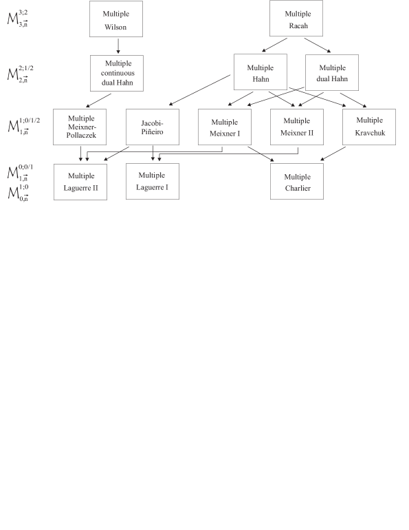
Figure 2: The (incomplete) multiple AT-Askey scheme

References

- [1] M. Abramowitz, I. A. Stegun, Handbook of Mathematical Functions, National Bureau of Standards, Washington, 1964; Dover, New York, 1972.
- [2] E. Andrews, R. Askey, R. Roy, Special Functions, Encyclopedia of Mathematics and its Applications 71, Cambridge University Press, Cambridge, 1999.
- [3] A. I. Aptekarev, Multiple orthogonal polynomials, J. Comput. Appl. Math. 99 (1998), 423-447.
- [4] A. I. Aptekarev, A. Branquinho, W. Van Assche, Multiple orthogonal polynomials for classical weights, Trans. Amer. Math. Soc. (to appear).
- [5] J. Arvesú, J. Coussement, W. Van Assche, Some discrete multiple orthogonal polynomials, to appear in J. Comput. Appl. Math. [on line: DOI 10.1016/S0377-0427(02)00597-6]
- [6] P. Borwein, T. Erdélyi, Polynomials and Polynomials Inequalities, Springer-Verlag, New York, Inc., 1995.
- [7] M. G. de Bruin, Simultaneous Padé approximation and orthogonality, in ’Polynomes Orthogonaux et Applications’ (C. Brezinski et al., eds.), Lecture Notes in Mathematics 1171, Springer-Verlag, Berlin, 1985, 74-83.
- [8] M. G. de Bruin, Some aspects of simultaneous rational approximation, in ’Numerical Analysis and Mathematical Modeling’, Banach Center Publications 24, PWN-Polish Scientific Publishers, Warsaw, 1990, 51-84.
- [9] T. S. Chihara, An Introduction to Orthogonal Polynomials, Gordon and Breach, New York, 1978.
- [10] J.G. van der Corput, Over eenige determinanten, Proc. Kon. Akad. Wetensch. Amsterdam 14 (1930), 1-44.
- [11] J.G. van der Corput, H.J. Duparc, Determinants and quadratic forms (first communication), Nederl. Akad. Wetensch. Proc. 49 (1946), 995-1002.
- [12] E. Coussement, W. Van Assche, Some properties of multiple orthogonal polynomails associated with Macdonald functions, J. Comput. Appl. Math. 133 (2001), no. 1-2, 253-261.
- [13] E. Coussement, W. Van Assche, Multiple orthogonal polynomials associated with the modified Bessel functions of the first kind, Constr. Approx. 19 (2003), 237-263.
- [14] E. Coussement, W. Van Assche, Some classical multiple orthogonal polynomials, J. Comput. Appl. Math. 127 (2001), 317-347.
- [15] A. Erdélyi, Higher Transcendental Functions I, II, McGraw-Hill, 1953.
- [16] H. Hochstadt, The Functions of Mathematical Physics, Dover Publications, Inc. 1986.
- [17] R. Koekoek, R. Swarttouw, The Askey-scheme of hypergeometric orthogonal polynomials and its -analogue, Reports of the faculty of Technical Mathematics and Informatics 98-17, 1998. (math.CA/9602214 at arXiv.org)
- [18] T. H. Koornwinder, Special orthogonal polynomial systems mapped onto each other by the Fourier-Jacobi transform, in ’Polynomes Orthogonaux et Applications’ (C. Brezinski et al., eds.), Lecture Notes in Mathematics 1171, Springer-Verlag, Berlin, 1985, 174-183.
- [19] A.B.J. Kuijlaars, A. Martinez-Finkelshtein, R. Orive, Orthogonality of Jacobi polynomials with general parameters, arXiv:math.CA/0301037v1, to appear in Electronic Transactions on Numerical Analysis.
- [20] K. Mahler, Perfect systems, Compositio Math. 19 (1968), 95-166.
- [21] C. S. Meijer, Zur Theorie der hypergeometrischen Funktionen, Indagationes Mathematicae, 1(1939) 100-114.
- [22] A.F. Nikishin, V.N. Sorokin, Rational Approximants and Orthogonality, Translations of Mathematical Monographs, 92, Amer. Math. Soc., Providence, RI (1991).
- [23] L. R. Piñeiro, On simultaneous Padé approximants for a collection of Markov functions, Vestnik Mosl. Univ., Ser. I (2) (1987), 67-70 (in Russian); translated in Moscow Univ. Math. Bull. 42 (2) (1987), 52-55.
- [24] H. M. Srivastava, Per W. Karlsson, Multiple Gaussian Hypergeometric Series, Ellis Horwood Series in Mathematics and its Applications, Horwood Chichester, New York, 1984.
- [25] G. Szegő, Orthogonal Polynomials, Amer. Math. Soc., Providence, RI, 1939, 4th edition 1975.
- [26] W. Van Assche, S.B. Yakubovich, Multiple orthogonal polynomials associated with Macdonald Functions, Integral Transform. Spec. Funct. 9 (2000), no. 3, 229-244.
- [27] J. A. Wilson, Some hypergeometric orthogonal polynomials, SIAM J. Math. Anal. 11 (1980), 690–701.
- [28] J. A. Wilson, Asymptotics for the polynomials, J. Approx. Theory 66 (1991), 58–71.