Abstract

We study the dynamics of $N$ point vortices on a rotating sphere. The Hamiltonian system becomes infinite dimensional due to the non-uniform background vorticity coming from the Coriolis force. We prove that a relative equilibrium formed of latitudinal rings of identical vortices for the non-rotating sphere persists to be a relative equilibrium when the sphere rotates. We study the nonlinear stability of a polygon of planar point vortices on a rotating plane in order to approximate the corresponding relative equilibrium on the rotating sphere when the ring is close to the pole. We then perform the same study for geostrophic vortices. To end, we compare our results to the observations on the southern hemisphere atmospheric circulation.

Keywords: point vortices, rotating sphere, relative equilibria, nonlinear stability, planar vortices, geostrophic vortices, Southern Hemisphere Circulation

AMS classification scheme number: 70E55, 70H14, 70H33

PACS classification scheme number: 45.20.Jj, 45.50.Jf, 47.20.Ky, 47.32.Cc

1 Introduction

The interest of studying point vortices on a rotating sphere is clearly geophysical. This may permit also to understand the motion of concentrated regions of vorticity on the surface of planets such as Jupiter [DL93]. The literature is now numerous on point vortices on a non-rotating sphere [B77, KN98, KN99, KN00, N00, PM98, LMR01, BC01, LP02] but only few papers consider a rotating sphere [F75, B77, B85, KR89, DP98]. In [F75], the interaction of three identical point vortices equally spaced on the same latitude is investigated via the $\beta$-plane approximation. It is shown — under some additional assumptions — that this configuration is an equilibrium, and that its linear stability depends on the strength of the vortices: linearly stable for a negative or a strongly positive strength, linearly unstable otherwise. In [B77], the equations of motion on a rotating sphere are given, while in [B85] the motion of a single point vortex is given. It appears that a single vortex moves westward and northward as a hurricane does. In [KR89], the approach is completely different from ours and [B77]; they proved the existence of relative equilibria formed of two or three vortices of possibly non-identical vorticities. In [DP98], they model the background vorticity coming from the rotation by latitudinal strips of constant vorticities and they study the motion of a vortex pair (point-vortex pair as well as patch-vortex pair). A vortex pair is a solution formed of two vortices with opposite sign vorticities rotating around the North pole. A vortex pair moving eastward or strongly westward is stable, unless the vortex sizes are too large. Different types of instabilities are described for weak westward pairs.

In this paper, we first recall some basics notions of geometric mechanics in Section 2. In particular, the notion of relative equilibrium is defined. In the cases of that paper, a relative equilibrium corresponds to a rigid rotation of $N$ point vortices about some axis. We then give the equations of motion for point vortices on a rotating sphere [B77] in Section 3. The Hamiltonian system is infinite dimensional due the background vorticity coming from the rotation of the sphere.

We prove that a relative equilibrium formed of latitudinal rings of the non-rotating system persists when the sphere rotates. From [LMR01] and [LP02], we know that the following arrangements of latitudinal rings are relative equilibria of the non-rotating system: $C_{Nv}(R,k_{p}p)$, $D_{Nh}(2R,k_{p}p)$, $D_{Nd}(R,R^{\prime},k_{p}p)$, and $D_{2Nh}(R_{e},k_{p}p)$ ($k_{p}$ is the number of polar vortices). See Figures 1, 2, and 3.

(a) $C_{4v}(R)$

(b) $C_{4v}(R,p)$

Figure 1: The $C_{nv}(R,k_{p}p)$ relative equilibria with $k_{p}=0,1$.

Figure 2: Relative equilibria $D_{4h}(2R)$ and $D_{4d}(R,R^{\prime})$.

Figure 3: Equatorial ($\pm$)ring $D_{2Nh}(R_{e})$.

In Section 4, we give the stability of relative equilibria $C_{Nv}(R)$ and $C_{Nv}(R,p)$ for three different approximations or limiting cases: point vortices on a rotating plane, geostrophic vortices, and point vortices on a non-rotating sphere. Indeed in that particular cases the system becomes finite dimensional and we can use the techniques of Section 2 to obtain both nonlinear and linear stability results. The stability is determined with a block diagonalization version of the Energy-momentum method [OR99, LP02] and the Lyapunov stability results are modulo $SO(2)$. In particular, we compute the (nonlinear) stability of a polygon formed of $N$ identical point vortices in the plane together with a central vortex of arbitrary vorticity in Appendix B. Our results differ from those of [CS99] but agree with the linear study of [MS71]. We also improve some stability results on geostrophic vortices of [MS71] proving that some linear stable configurations are actually Lyapunov stable.

The paper ends with a discussion on the Southern Hemisphere Circulation and its relationship with vortices.

2 Geometric mechanics

We recall thereafter some basics notions of geometric mechanics. We refer to [MR94, Or98] for further details.

Let $G$ be a connected Lie group acting smoothly on a symplectic manifold $(\mathcal{P},\varpi)$. Consider an Hamiltonian dynamical system $(\mathcal{P},\varpi,H)$ with momentum map $J:\mathcal{P}\to\mathfrak{g}^{*}$ such that the Hamiltonian vector field $X_{H}$ and the momentum map are $G$-equivariant. A point $x_{e}\in\mathcal{P}$ is called a relative equilibrium if for all $t$ there exists $g_{t}\in G$ such that $x_{e}(t)=g_{t}\cdot x_{e}$, where $x_{e}(t)$ is the dynamic orbit of $X_{H}$ with $x_{e}(0)=x_{e}$. In other words, the trajectory is contained in a single group orbit. A relative equilibrium $x_{e}\in\mathcal{P}$ is a critical point of the augmented Hamiltonian:

$$H_{\xi}(x)=H(x)-\left<J(x)-\mu,\xi\right>$$

for some $\xi\in\mathfrak{g}$. The vector $\xi$ is unique if the action of $G$ is locally free, and is called the angular velocity of $x_{e}$.

In the case of point vortices on a rotating sphere, we will have $G=SO(2)$. Hence relative equilibria are rigid rotations with angular velocity $\xi\in\mathfrak{so}(2)\simeq\mathbb{R}$ around the axis of rotation of the sphere.

The Hamiltonian is $G$-invariant, but may have additional symmetries. Denote by $\hat{G}$ the group of symmetries of the Hamiltonian. For example, in the case of $N$ identical point vortices on a non-rotating sphere, one has $G=SO(3)\times S_{N}$ and $\hat{G}=O(3)\times S_{N}$ [LMR01]. Let the fixed point set of a subgroup $K$ of $\hat{G}$ be:

$$\mathop{\rm Fix}(K,\mathcal{P})=\{x\in\mathcal{P}\mid g\cdot x=x,\forall g\in K\}.$$

The following theorem permits to determine relative equilibria, it is a corollary of the Principle of Symmetric Criticality of Palais [P79].

Theorem 2.1

Let $K$ be a subgroup of $\hat{G}$, $x\in\mathop{\rm Fix}(K,\mathcal{P})$ and $\mu=J(x)$. Assume that $\hat{G}$ is compact. If $x$ is an isolated point in $\mathop{\rm Fix}(K,\mathcal{P})\cap J^{-1}(\mu)$, then $x$ is a relative equilibrium.

Note that this result depends only on the symmetries, the phase space and the momentum map, and not depends on the form of the Hamiltonian. A relative equilibrium obtained with that result is said to be a large symmetry relative equilibrium since its isotropy subgroup must be large.

To compute the stability of relative equilibria, we use the Energy momentum method: let $x_{e}$ be a relative equilibrium, $\mu=J(x_{e})\in\mathfrak{g}^{*}$ and $\xi$ be its angular velocity. The method consists first to determine the symplectic slice

$$\mathcal{N}=T_{x_{e}}(G_{\mu}\cdot x_{e})^{\bot}\cap\mathop{\rm Ker}DJ(x_{e})$$

where

$$G_{\mu}=\{g\in G\mid\mathop{\rm Coad}\nolimits_{g}\cdot\mu=\mu\}.$$

The second step consists to examine the definitness of $d^{2}H_{\xi}|_{\mathcal{N}}(x_{e})$, and apply the following result [Pa92, OR99] which holds in particular if $G$ is compact:

If $d^{2}H_{\xi}|_{\mathcal{N}}(x_{e})$ is definite, then $x_{e}$ is Lyapunov stable modulo $G_{\mu}$.

In Section 4.1, we will consider vortices in the plane (point vortices and geostrophic vortices), the symmetry group $G$ is $SE(2)$ or $SO(2)$ depending on whether the plane is rotating. However we will forget translational symmetries since $SE(2)$ is not compact, hence we take $G=SO(2)$ and the previous result holds. Moreover we have $G_{\mu}=SO(2)$ for all $\mu\in\mathfrak{so}(2)^{*}\simeq\mathbb{R}$. In Section 4.2, the sphere is non-rotating, thus the symmetry group is $G=SO(3)$ [LP02, LMR]. We have $SO(3)_{\mu}=SO(2)$ for $\mu\neq 0$, and $SO(3)_{\mu=0}=SO(3)$. Since we will consider only relative equilibria with a non-zero momentum $\mu$ for that section, Lyapunov stable will mean Lyapunov stable modulo $SO(2)$ throughout that paper.

The linear stability is investigated calculating the eigenvalues of the linearization in the symplectic slice, that is of $L_{\mathcal{N}}=\Omega_{\mathcal{N}}^{\flat-1}d^{2}H_{\xi}|_{\mathcal{N}}(x_{e})$ where $\Omega_{\mathcal{N}}^{\flat}$ is the matrix of $\varpi|_{\mathcal{N}}$.

The symplectic slice $\mathcal{N}$ is a $G_{x_{e}}$-invariant subspace. Hence we can perform an $G_{x_{e}}$-isotypic decomposition of $\mathcal{N}$, this permits to block diagonalize the matrices $d^{2}H_{\xi}|_{\mathcal{N}}(x_{e})$ and $L_{\mathcal{N}}$, their eigenvalues are then easier to compute and we can conclude about both Lyapunov and linear stability. A basis of the symplectic slice in which these matrices block diagonalize is called a symmetry adapted basis. The symmetry adapted bases do not depend on the particular form of the system, they depend only on the symmetries of the system.

The different steps of the method are widely detailed in [LP02] which is a study on point vortices on a non-rotating sphere.

A relative equilibrium $x_{e}$ is said to be elliptic if it is spectrally stable with $d^{2}H_{\xi}|_{\mathcal{N}}(x_{e})$ not definite. An elliptic relative equilibrium may be Lyapunov stable, but this can not be proved via the Energy-momentum method (but KAM theory may work). Note also that an elliptic relative equilibrium becomes linearly unstable when some dissipation is added to the system [DR02].

3 Equations of motion and relative equilibria

In this section we consider $N$ point vortices on a unit sphere rotating with a constant angular velocity $\Omega$ around the axis $(Oz)$. Hence the $SO(3)$ symmetry of the non-rotating system breaks to $SO(2)$. The Coriolis force induces a continuous vorticity $\omega_{\Omega}$ on the sphere: $\omega=\omega_{0}+\omega_{\Omega}$ where $\omega_{0}=\sum_{i}\lambda_{i}\delta(x-x_{i})$, $\lambda_{i}$ is the vorticity of the vortex $x_{i}$, and $\omega_{\Omega}(t=0)=2\Omega\cos\theta$. The continuous vorticity is not uniform and thus interacts a priori with the singular vorticity i.e. the vortices. This interaction makes $\omega_{\Omega}$ a function of time. For example, without any vortices $\omega=\omega_{\Omega}=2\Omega\cos\theta$ is a steady solution.

The stream function $\psi$ satisfies $\Delta\psi=\omega$. Hence $\psi=G\ast\omega$ where $G$ is the Green function on the sphere $G(x,x^{\prime})=1/(4\pi)\ln(1-x\cdot x^{\prime})$, and we obtain the following expression for the stream function:

$$\psi=\frac{1}{4\pi}\sum_{i=1}^{N}\lambda_{i}\ln(1-x\cdot x_{i})+G\ast\omega_{\Omega}.$$

The equations governing the motion of the vortices are therefore [B77]:

$$\dot{\theta}_{i}=\sum_{j=1,j\neq i}^{N}\lambda_{j}\frac{\sin\theta_{j}\sin(\phi_{i}-\phi_{j})}{1-x_{i}\cdot x_{j}}+\frac{1}{\sin\theta_{i}}\frac{\partial G\ast\omega_{\Omega}}{\partial\phi_{i}}(\theta_{i},\phi_{i})$$

$$\sin\theta_{i}\ \dot{\phi}_{i}=-\sum_{j=1,j\neq i}^{N}\lambda_{j}\frac{\sin\theta_{i}\cos\theta_{j}-\sin\theta_{j}\cos\theta_{i}\cos(\phi_{i}-\phi_{j})}{1-x_{i}\cdot x_{j}}-\frac{\partial G\ast\omega_{\Omega}}{\partial\theta_{i}}(\theta_{i},\phi_{i})$$

for all $i=1,\dots,N$. Moreover, the vorticity satisfies $\partial_{t}\omega+(u\cdot\nabla)\omega=0$ (Euler), $u$ being the velocity, and this equation can be written equivalently with a Poisson bracket:

$$\dot{\omega}=\{\omega,\psi\}$$

where

$$\{f,g\}=\frac{\partial f}{\partial\cos\theta}\frac{\partial g}{\partial\phi}-\frac{\partial f}{\partial\phi}\frac{\partial g}{\partial\cos\theta}$$

for two smooth functions $f,g$ on the sphere. The full dynamical system is therefore:

$$\dot{\theta}_{i}=\sum_{j=1,j\neq i}^{N}\lambda_{j}\frac{\sin\theta_{j}\sin(\phi_{i}-\phi_{j})}{1-x_{i}\cdot x_{j}}+\frac{1}{\sin\theta_{i}}\frac{\partial G\ast\omega_{\Omega}}{\partial\phi_{i}}(\theta_{i},\phi_{i})$$

$$\sin\theta_{i}\ \dot{\phi}_{i}=-\sum_{j=1,j\neq i}^{N}\lambda_{j}\frac{\sin\theta_{i}\cos\theta_{j}-\sin\theta_{j}\cos\theta_{i}\cos(\phi_{i}-\phi_{j})}{1-x_{i}\cdot x_{j}}-\frac{\partial G\ast\omega_{\Omega}}{\partial\theta_{i}}(\theta_{i},\phi_{i})$$

$$\dot{\omega}_{\Omega}=\{\omega_{\Omega},\psi\}$$

since the strengths of the vortices are constant.

Remark. The vorticity must satisfy $\int\omega\;dS=0$ from Stoke’s theorem. It should be noted that when the sum $\Lambda=\sum\lambda_{i}$ is non-zero, then the stream function remains as before taking $\omega_{0}=-\Lambda/(4\pi)+\sum_{i}\lambda_{i}\delta(x-x_{i})$. Since $\omega_{0}$ satisfies $\int\omega_{0}\;dS=0$, it follows that $\int\omega\;dS=0$ when $\omega_{\Omega}=2\Omega\cos\theta$.

It is easy to verify that the following quantity (total kinetic energy) is conserved and serves as a Hamiltonian:

$$H = \frac{1}{2}\int_{S^{2}}\omega\cdot\psi\ dS=\frac{1}{2}\int_{S^{2}}\omega\cdot G\ast\omega\ dS$$

$$= \frac{1}{4\pi}\sum_{i<j}\lambda_{i}\lambda_{j}\ln(1-x_{i}\cdot x_{j})+\frac{1}{2}\sum_{k=1}^{N}\lambda_{k}G\ast\omega_{\Omega}(\theta_{k},\phi_{k})$$

$$+\frac{1}{2}\int_{S^{2}}\int_{S^{2}}\omega_{\Omega}(\theta,\phi)\omega_{\Omega}(\theta^{\prime},\phi^{\prime})G(\theta,\phi,\theta^{\prime},\phi^{\prime})dSdS^{\prime}.$$

Let $SO(2)$ be the group of rotations with as axis the axis of rotation of the sphere, and consider the diagonal action of $SO(2)$ on the product of $N$ spheres. Clearly the continuous vorticity satisfies

$$\omega_{\Omega}(g\cdot\theta,g\cdot\phi,g\cdot\theta_{1},g\cdot\phi_{1},\dots,g\cdot\theta_{N},g\cdot\phi_{N})=\omega_{\Omega}(\theta,\phi,\theta_{1},\phi_{1},\dots,\theta_{N},\phi_{N})$$

for all $g\in SO(2)$. It follows that $H$ is $SO(2)$-invariant and the dynamical system is $SO(2)$-equivariant.

Due to the continuous vorticity, the phase space $\mathcal{P}$ becomes infinite dimensional:

$$\mathcal{P}=\{(x_{1},\dots,x_{N})\in S^{2}\times\cdots\times S^{2}\mid x_{i}\neq x_{j}\ \mbox{if}\ i\neq j\}\times\mathcal{F}(S^{2})$$

where $\mathcal{F}(S^{2})$ is the set of smooth functions on the sphere.

The following vector (momentum vector) is conserved and thus provides three conserved quantities [B77]:

$$\vec{M} = \int_{S^{2}}\omega\cdot\vec{x}\ dS$$

$$= \sum_{j=1}^{N}\lambda_{j}\;x_{j}+\left(\begin{array}[]{l}\int_{S^{2}}\omega_{\Omega}(\theta,\phi)\sin\theta\cos\phi\ dS\\ \int_{S^{2}}\omega_{\Omega}(\theta,\phi)\sin\theta\sin\phi\ dS\\ \int_{S^{2}}\omega_{\Omega}(\theta,\phi)\cos\theta\ dS\end{array}\right).$$

The term $\sum\lambda_{j}x_{j}$ corresponds to the moment map for point vortices on a non-rotating sphere [LMR01]. Indeed in the case of the non-rotating sphere, the dynamical system is $SO(3)$-equivariant, and this leads to three conserved quantities since $SO(3)$ is of dimension three. In the case of the rotating sphere the system is only $SO(2)$-equivariant, hence the symmetries provide only one conserved quantity (which is the $z$-component of $\vec{M}$). Actually, the three conserved quantities come from a general property of $2D$ incompressible and inviscid fluid flows on compact and simply connected surfaces which states that the vector $\int\omega\cdot\vec{x}\;dS$ is conserved, no matter the symmetries of the surface we have [B]. That vector and the momentum map simply coincide in the case of a non-rotating sphere.

We would like to know if the relative equilibria found on the non-rotating sphere persist when the sphere rotates. We call an N-ring a latitudinal regular polygon formed of $N$ identical vortices. The following theorem show that relative equilibria formed of $N$-rings (together with possibly some polar vortices) persist.

Theorem 3.1

Let $x_{e}$ be a relative equilibrium of the non-rotating system, with angular velocity $\xi_{0}$, formed of $m$ $N_{m}$-rings ($N_{m}\geq 2$) together with possibly some polar vortices. Then $(x_{e},\omega_{\Omega}(t)=2\Omega\cos\theta)$ is a relative equilibrium of the rotating system with angular velocity $\xi=\xi_{0}+\Omega$.

Corollary 3.2

The relative equilibria

$$C_{Nv}(R,k_{p}p),\ D_{Nh}(2R,k_{p}p),\ D_{Nd}(R,R^{\prime},k_{p}p),\ D_{2Nh}(R_{e},k_{p}p)$$

persist when the sphere rotates.

Proof.  Let $(x_{e},\xi_{0})$ be a relative equilibrium of the non-rotating system formed of $k_{r}$ $N_{k}$-rings, a polar vortex being considered as a $1$-ring. Hence

$$\dot{\theta}_{i} = \frac{1}{\sin\theta_{i}}\frac{\partial G\ast\omega_{\Omega}}{\partial\phi_{i}}(\theta_{i},\phi_{i})$$

$$\dot{\phi}_{i} = \xi_{0}-\frac{1}{\sin\theta_{i}}\frac{\partial G\ast\omega_{\Omega}}{\partial\theta_{i}}(\theta_{i},\phi_{i})$$

for all $i=1,\dots,N$.

Let the continuous vorticity be $\omega_{\Omega}(t)=2\Omega\cos\theta$ for all time $t$. We have $\frac{\partial G\ast\omega_{\Omega}}{\partial\phi_{i}}=0$ since $\int G(\theta,,\phi,\theta_{i},\phi_{i})d\phi$ does not depend on $\phi_{i}$, and

$$\frac{\partial G\ast\omega_{\Omega}}{\partial\theta_{i}} = \frac{\Omega}{4\pi}\int_{\theta=0}^{\pi}\sin 2\theta\int_{\phi=0}^{2\pi}\frac{\cos\theta\sin\theta_{i}-\sin\theta\cos\theta_{i}\cos(\phi-\phi_{i})}{1-\cos\theta\cos\theta_{i}-\sin\theta\sin\theta_{i}\cos(\phi-\phi_{i})}d\phi d\theta$$

$$= \frac{\Omega}{2}\int_{\theta=0}^{\pi}\sin 2\theta\left[\frac{\cos\theta\sin\theta_{i}}{|\cos\theta-\cos\theta_{i}|}+\frac{\cos\theta_{i}}{\sin\theta_{i}}\left(1-\frac{1-\cos\theta\cos\theta_{i}}{|\cos\theta-\cos\theta_{i}|}\right)\right]d\theta.$$

And we obtain after some calculus that $\frac{\partial G\ast\omega_{\Omega}}{\partial\theta_{i}}=-\Omega\sin\theta_{i}$.

Thus we proved that $\dot{\theta}_{i}=0$ and $\dot{\phi}_{i}=\xi_{0}+\Omega$ for all $i=1,\dots,N$. It remains then to prove that $\dot{\omega}_{\Omega}=0$. One has $\dot{\omega}_{\Omega}=\{\omega_{\Omega},\psi\}=2\Omega\frac{\partial\psi}{\partial\phi}$. Since $\frac{\partial G\ast\omega_{\Omega}}{\partial\phi}=0$, it follows that

$$\frac{\partial\psi}{\partial\phi}=\sum_{k=1}^{k_{r}}\sum_{j=1}^{N_{k}}\lambda_{k}\frac{\sin\theta\sin\theta_{k}\sin(\phi-\phi_{j,k})}{1-\cos\theta\cos\theta_{k}-\sin\theta\sin\theta_{k}\cos(\phi-\phi_{j,k})}$$

where $\lambda_{k}$ and $\theta_{k}$ are respectively the vorticity and the co-latitude of the ring $k$, and $\phi_{j,k}=\epsilon_{k}+2\pi(j-1)/N$. It can be shown that this sum vanishes (see Appendix A), hence $\dot{\omega}_{\Omega}=0$ and $(x_{e},\omega_{\Omega}(t)=2\Omega\cos\theta)$ is a relative equilibrium of the rotating system with angular velocity $\xi=\xi_{0}+\Omega$. $\Box$

Remark. In order to prove existence of relative equilibria, we may think to use the Principle of Symmetric Criticality of Section 2. The Principle holds since $SO(2)$ is compact, however the fixed point sets $\mathop{\rm Fix}(C_{N},\mathcal{P})$ are infinite dimensional, it is therefore quite a task to find relative equilibria with that method.

4 Stability of relative equilibria on the rotating sphere

In this section, we unfortunately do not compute the stability of the relative equilibria determined in the previous section. Indeed the Hamiltonian system is here infinite dimensional and the method described in Section 2 work only for finite dimensional Hamiltonian systems. Hence we will give in this section the stability of different approximations or limiting cases of the “rotating sphere problem” which lead to a finite dimensional Hamiltonian system.

4.1 Vortices on a rotating plane

We consider point vortices on a rotating plane in order to approximate the $C_{Nv}(R)$ and $C_{Nv}(R,p)$ relative equilibria on a rotating sphere when the ring is close to the pole. This approximation can be done in two different manners: the “classical” point vortices on a rotating plane, and the “geostrophic” vortices [S43]. The equivalent of the $C_{Nv}(R,p)$ arrangement on the plane is the arrangement $C_{N}(R,p)$: a regular polygon formed of $N$ vortices of strength $1$ together with a central vortex of strength $\lambda$. When there is no central vortex, the configuration is denoted $C_{N}(R)$ and corresponds to the $C_{Nv}(R)$ arrangement on the sphere (see Figure 4). We assume that $N\geq 3$ since the cases $N=2$ are degenerate due the colinearity of the arrangements.

(a) $C_{4}(R)$

(b) $C_{4}(R,p)$

Figure 4: The $C_{N}(R,k_{p}p)$ planar relative equilibria.

Point vortices on a rotating plane.
Consider a system of point vortices on a plane rotating with a constant angular velocity $\Omega$ around its normal axis. Contrary to the rotating sphere, the continuous vorticity induced by the rotation is here uniform, thus the continuous vorticity does not interact with the point vortices. The dynamics of point vortices on the rotating plane is therefore similar to that for the non-rotating plane as the following proposition shows.

Denote a relative equilibrium $x_{e}=(z_{1},\dots,z_{N})\in\mathbb{C}^{N}$ with angular velocity $\xi$ by $(x_{e},\xi)$ and set the origin of the plane to be the centre of the rotation. Recall that $\Lambda$ is the sum of the vorticities, that is $\Lambda=\sum_{i}\lambda_{i}$.

Theorem 4.1

If $(x_{e},\xi)$ is a relative equilibrium of the non-rotating plane such that $\sum\lambda_{j}z_{j}=0$ and $\Lambda\neq 0$, then $(x_{e},\xi+\Omega)$ is a relative equilibrium of the rotating plane. Moreover $(x_{e},\xi+\Omega)$ satisfies the stability properties of $(x_{e},\xi)$ (as elements of $\mathcal{P}/SO(2)$).

Proof.  The continuous vorticity induced by the rotation of the plane is $\omega_{\Omega}(x,y)=2\Omega$, thus the distribution of vorticity for $N$ point vortices $z_{j}=\rho_{j}\exp(i\phi_{j})$, $j=1,\dots,N$ is given by $\omega=2\Omega+\sum_{j}\lambda_{j}\ \delta(z-z_{j})$. It follows that the Hamiltonian is

$$H=\frac{\Omega}{2}\sum_{j}\lambda_{j}\rho_{j}^{2}+H_{0},$$

where $H_{0}$ is the Hamiltonian for the non-rotating plane (see Appendix B).

Since $\lambda_{j}\dot{\rho}_{j}=-\frac{1}{\rho_{j}}\frac{\partial H}{\partial\phi_{j}}$ and $\lambda_{j}\dot{\phi}_{j}=\frac{1}{\rho_{j}}\frac{\partial H}{\partial\rho_{j}}$, the dynamical system is given by

$$\left(\begin{array}[]{c}\dot{\rho}_{j}\\ \dot{\phi}_{j}\end{array}\right)=\left(\begin{array}[]{c}0\\ \Omega\end{array}\right)+\left(\begin{array}[]{c}-\frac{1}{\lambda_{j}\rho_{j}}\frac{\partial H_{0}}{\partial\phi_{j}}\\ \frac{1}{\lambda_{j}\rho_{j}}\frac{\partial H_{0}}{\partial\rho_{j}}\end{array}\right).$$

Since $\sum\lambda_{j}z_{j}=0$ and $\Lambda\neq 0$, one can show that the relative equilibrium of the non-rotating plane $(x_{e},\xi)$ satisfies

$$\frac{\partial H_{0}}{\partial\phi_{j}}=0,\ \frac{1}{\lambda_{j}\rho_{j}}\frac{\partial H_{0}}{\partial\rho_{j}}=\xi$$

for all $j$ ($\Lambda\neq 0$ is required to insure the existence of the “barycentre” $\sum_{j}\lambda_{j}z_{j}/\Lambda$). Hence $(\tilde{x}_{e},\tilde{\xi})$ with $\tilde{x}_{e}=x_{e}$ and $\tilde{\xi}=\Omega+\xi$ is a relative equilibrium of the rotating plane.

If a vortex $z_{j}$ of the relative equilibrium $x_{e}$ is at the origin (a central vortex), this discussion is not valid due to the degeneracy of polar coordinates at the origin, we then use cartesian coordinates and find the same conclusions.

We are interested in stability in $\mathcal{P}/SO(2)$ (stability modulo $SO(2)$) where $SO(2)$ is the group of rotations around the origin. The “rotating” dynamical system is $SO(2)$-equivariant. The momentum map coming from the $SO(2)$ symmetry is $J=\sum_{j}\lambda_{j}\rho_{j}^{2}/2\in\mathbb{R}\simeq\mathfrak{so}(2)^{\star}$ (see Appendix B), thus $H=H_{0}+\Omega J$. Hence

$$d^{2}H_{\tilde{\xi}}(\tilde{x}_{e})=d^{2}H(x_{e})-(\Omega+\xi)d^{2}J(x_{e})=d^{2}H_{0}(x_{e})-\xi d^{2}J(x_{e})=d^{2}{H_{0}}_{\xi}(x_{e}).$$

Moreover, the symplectic slice is the same for both the rotating and the non-rotating cases, since the stability is investigated in $\mathcal{P}/SO(2)$ (and not in $\mathcal{P}/SE(2)$ as we could do for the non-rotating case). The stability statement follows. $\Box$

Remark. The previous result is actually due to the fact that the Hamiltonian $H_{0}$ is perturbed by a function $J^{\Omega}(x)=\left<J(x),\Omega\right>$ where $J$ is a momentum map of a symmetry group $G$ of $H_{0}$, and $\Omega\in\mathfrak{g}$. The Hamiltonian $J^{\Omega}$ is a collective Hamiltonian (that is a function of $J$), see [GS84] for a general study of collective Hamiltonians.

Consequently, all relative equilibria of the non-rotating plane formed of regular polygons persist to be relative equilibria when the plane rotates, provided that the polygons are cocentric with centre of the rotation. In particular, the $C_{N}(R)$ and $C_{N}(R,p)$ relative equilibria persist (the centre of the ring being the centre of the rotation). For relative equilibria formed of several regular polygons, we refer to [LR96] in which a stability study is also given for some particular configurations.

We can now give stability results for the $C_{N}(R)$ and $C_{N}(R,p)$ relative equilibria thanks to the stability study of $C_{N}(R)$ relative equilibria [CS99] on the non-rotating plane and a theorem proved in Appendix B.

Proposition 4.2

The $C_{N}(R)$ relative equilibria on a rotating plane are Lyapunov stable if $N\leq 7$ and linearly unstable otherwise.

Let $\varepsilon_{N}=+1$ if $N$ is even, and $\varepsilon_{N}=0$ if $N$ is odd.

Theorem 4.3

The $C_{N}(R,p)$ relative equilibria with $N\geq 4$ on a plane (rotating or not) are Lyapunov stable if $\max(0,(N^{2}-8N+7+\varepsilon_{N})/16)<\lambda<(N-1)^{2}/4$, elliptic if $(N^{2}-8N+7+\varepsilon_{N})/16<\lambda<0$, and linearly unstable if the previous conditions are not satisfied. The $C_{3}(R,p)$ relative equilibria are Lyapunov stable if $0<\lambda<1$, elliptic if $\lambda<0$, and linearly unstable if $\lambda>1$.

We have $(N^{2}-8N+7+\varepsilon_{N})/16<0$ if and only if $N\leq 6$, hence there exists some linearly stable configurations with a negative central vorticity only for $N\leq 6$.

Proof.  The stability results of $C_{N}(R,p)$ relative equilibria on a non-rotating plane are given in Appendix B since the proof is quite long. These results will hold for a rotating plane by Theorem 4.1. $\Box$

Remark. The Lyapunov stability of $C_{7}(R)$ (the Thomson heptagon) is not proved with an energetic method. Indeed the Hessian is not definite at this relative equilibrium, one needs to go to the fourth order to determine the Lyapunov stability [M78, CS99].

Geostrophic vortices.
In his paper [S43], Stewart considered a single layer of fluid of constant density on a rotating disc in order to model the atmosphere of the Earth. Let $\Omega$ be the constant angular velocity of the disc, $z$ be the complex coordinate on the rotating disc, $h_{0}$ be the uniform depth of the fluid at rest and $g$ be the acceleration due to gravity. By means of the geostrophic wind equations, he found that the stream function corresponding to a vortex at $z_{0}$ with vorticity $\lambda$ is

$$\Psi=\lambda K_{0}(\kappa|z-z_{0}|)$$

where $\kappa=2\Omega/\sqrt{gh_{0}}$ and $K_{0}$ is the Bessel function of the second kind. Such a vortex is called a geostrophic (or Bessel) vortex. The Hamiltonian for a system of $N$ geostrophic vortices $z_{1},\dots,z_{N}$ with vorticities $\lambda_{1},\dots,\lambda_{N}$ is

$$H=\sum_{i<j}\lambda_{i}\lambda_{j}K_{0}(\kappa|z_{i}-z_{j}|).$$

Note that a geostrophic vortex is almost a planar $\kappa^{-1}$-Euler vortex, the parameter $\kappa^{-1}$ is the horizontal length scale of the geostrophic vortex. In the case of the Earth $\kappa^{-1}$ is about $2000$ kms. If we rescale the radius of the Earth to be $1$ as the spheres previously considered, $\kappa$ is about $3$. Note also that the limiting case $\kappa=0$ corresponds to logarithmic vortices, that is to classical point vortices.

Since the Hamiltonian for the geostrophic vortices has the same symmetries as the Hamiltonian for the planar point vortices, we follow Section 2 to determine large symmetry relative equilibria and study their stability: it is easy to show that $C_{N}(R)$ and $C_{N}(R,p)$ configurations are large symmetry relative equilibria for the system of planar point vortices, and to find the symmetry adapted basis. The symmetry adapted basis for $C_{N}(R,p)$ is given in Appendix B, while the one for $C_{N}(R)$ is easily deduced from the former. These bases are similar to those for the $C_{Nv}(R)$ and $C_{Nv}(R,p)$ configurations of point vortices on a sphere [LMR].

We set the value of the vorticity of the ring to be $1$. The stability results are given in Proposition 4.4 for $C_{N}(R)$ geostrophic relative equilibria and in Figure 5 for $C_{N}(R,p)$ geostrophic relative equilibria. The linear stability results were already found by Morikawa and Swenson [MS71] by means of a numerical computation of the eigenvalues of the linearization. Here we compute numerically the eigenvalues of the diagonal blocks of the Hessian and the linearization, and thus conclude about both formal (hence Lyapunov) and linear stability. The results of this paper agree with their results except for the right stability frontiers where they differ slightly. This is probably due to a lack of accuracy. The advantage of the method described here is that we know that both the Hessian and the linearization block diagonalize, hence it is not necessary to compute the nil blocks (gain of time), and we know that the components in it are all zero and this contributes to improve the accuracy of the eigenvalues (indeed, if we compute numerically the components of the nil blocks, we find for example $10^{-13}$ instead of zero, and this leads finally to a lack of accuracy in the computations of the eigenvalues).

Proposition 4.4

The stability of the geostrophic $C_{N}(R)$ relative equilibria depends on $N$ and $\kappa$ as follows:

• $N\geq 7$: linearly unstable for all $\kappa>0$;

• $N=6$: Lyapunov stable for $\kappa\in[0,1.28]$, linearly unstable otherwise;

• $N=5$: Lyapunov stable for $\kappa\in[0,3.75]$, elliptic otherwise;

• $N=3,4$: Lyapunov stable for all $\kappa\geq 0$.

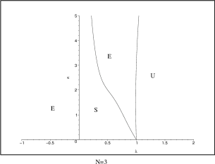
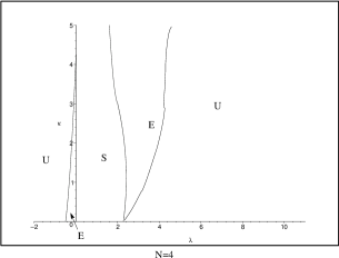
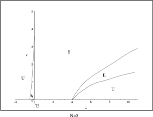
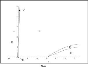
Figure 5: Stability results for geostrophic $C_{N}(R,p)$ relative equilibria. A relative equilibrium can be formally stable (S), linearly unstable (U), elliptic (E). The diagrams for $N\geq 8$ are similar to that for $N=11$.

Instability on the left part of the figures is due to the ring, while instability in right part is due to the central vortex. For $N=3$, the linear stability frontier of the central vortex (the right one) is almost a vertical line for $\kappa\in[0,5]$, that is $\kappa$ in that range has almost no influence on the linear stability of the central vortex. For $N=4,\dots,7$, the stability frontier of the ring (the left one) has the same property. On the other hand, the stability frontiers of the central vortex (the two on the right) for $N>4$ depend on $\kappa$. Note that the notion of “dependence” is linked to the scale of the figure for $N=5$, that is $(\kappa,\lambda)\in[0,5]\times[-2,10]$.

For $N\leq 7$, almost every relative equilibrium stable for $\kappa=0$ is stable for $\kappa\in[0,5]$ . Thus if a point vortices $C_{N}(R,p)$ relative equilibrium is stable, then so does the corresponding geostrophic relative equilibria. The point vortices system is therefore a good model to determine the stability (not instability) for $N\leq 7$. This becomes less and less true as $N$ increases. Indeed the greater is $N$, the more the stability depends on $\kappa$.

4.2 Stability results for $\Omega=0$

In this section, we give the stability results for the $C_{Nv}(R)$ and $C_{Nv}(R,p)$ relative equilibria on the non-rotating sphere.

The following theorem was proved first in term of linear stability in [PD93], and recently in term of Lyapunov stability in [LMR] and [BC01] by different ways.

Theorem 4.5

The stability of the ring of $N$ identical vortices depends on $N$ and the latitude as follows:

N=2

is Lyapunov stable at all latitudes;

N=3

is Lyapunov stable at all latitudes;

N=4

is Lyapunov stable if $\cos^{2}\theta_{0}>1/3$, and linearly unstable if the inequality is reversed;

N=5

is Lyapunov stable if $\cos^{2}\theta_{0}>1/2$, and linearly unstable if the inequality is reversed;

N=6

is Lyapunov stable if $\cos^{2}\theta_{0}>4/5$, and linearly unstable if the inequality is reversed;

N$>$6

is always linearly unstable,

where $\theta_{0}$ is the co-latitude of the ring.

The stability of $C_{Nv}(R,p)$ relative equilibria is given in the next theorem and illustrated by Figures 6 and 7. We assume that the polar vortex is at the North pole without loss of generality, and that the momentum of the relative equilibrium is non-zero. Let $\theta_{0}$ be the co-latitude of the ring.

Theorem 4.6 (Laurent-Polz, Montaldi, Roberts [LMR])

A $C_{2v}(R,p)$ relative equilibrium is Lyapunov stable if

$$(1+2\cos\theta_{0})[(1+\cos\theta_{0})^{2}\lambda+\cos\theta_{0}(2+3\cos\theta_{0})]<0.$$

and linearly unstable if the inequality is reversed.
A $C_{3v}(R,p)$ relative equilibrium is Lyapunov stable if $a\lambda(\lambda+n\cos\theta_{0})(\lambda-\lambda_{1})<0$, and spectrally unstable if and only if

$$8a\lambda>(n\sin^{2}\theta_{0}+4(n-1)\cos\theta_{0})^{2}.$$

A $C_{Nv}(R,p)$ relative equilibrium with $N\geq 4$

(i) is spectrally unstable if and only if

$$\lambda<\lambda_{0}\ \ \mbox{or}\ \ 8a\lambda>(N\sin^{2}\theta_{0}+4(N-1)\cos\theta_{0})^{2},$$

(ii) is Lyapunov stable if

$$\lambda>\lambda_{0}\ \ \mbox{and}\ \ a\lambda(\lambda+N\cos\theta_{0})(\lambda-\lambda_{1})<0,$$

where

$$\begin{array}[]{lll}a&=&(N\cos\theta_{0}-N+2)(1+\cos\theta_{0})^{2}\\ \lambda_{1}&=&(N-1)\cos\theta_{0}\;(N\sin^{2}\theta_{0}+2(N-1)\cos\theta_{0})/a\\ \lambda_{0}&=&(c_{N}-(N-1)(1+\cos^{2}\theta_{0}))/(1+\cos\theta_{0})^{2}\\ c_{N}&=&\cases{N^{2}/4&if $N$ is even,\cr(N^{2}-1)/4&if $N$ is odd.}\end{array}$$

Let $x_{e}$ be a $C_{Nv}(R)$ or $C_{Nv}(R,p)$ relative equilibrium on a sphere rotating with angular velocity $\Omega$. By the theory of perturbations, there exists a neighborhood $U$ of zero, $U\subset\mathbb{R}$, such that for all $\Omega\in U$, $x_{e}$ has the stability of the corresponding relative equilibrium on the non-rotating sphere. Hence the stability results of the two previous theorem persist in a neighborhood of zero for $\Omega$.

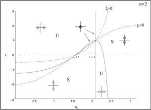
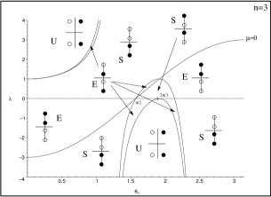
Figure 6: Bifurcation diagrams for $C_{2v}(R,p)$ and $C_{3v}(R,p)$ relative equilibria. The circles represent the eigenvalues of the mode $1$. A relative equilibrium can be Lyapunov stable (S), linearly unstable (U), elliptic (E).

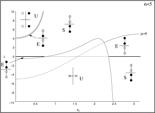
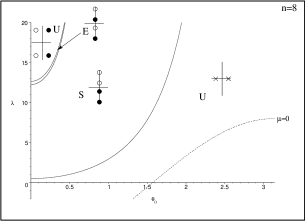
Figure 7: Bifurcation diagrams for $C_{Nv}(R,p)$ relative equilibria. The bifurcation diagrams for $N\geq 7$ are similar to that for $N=8$, while those for $N=4,6$ are similar to that for $N=5$. The circles represent the eigenvalues of the mode $1$, while the cross represent those of the mode $[N/2]$. A relative equilibrium can be Lyapunov stable (S), linearly unstable (U), elliptic (E).

4.3 Conclusions

From the results of that section, one can reasonably think that for a small angular velocity $\Omega$ the relative equilibrium $C_{Nv}(R)$ with a small co-latitude $\theta_{0}$ (that is the ring is close to the pole) is Lyapunov stable for $N\leq 5$, while it is linearly unstable for $N\geq 8$. The cases $N=6$ and $N=7$ are less clear since the stability for $N=6$ depends on the parameter $\kappa$ in Proposition 4.4, and the case $N=7$ is stable or unstable depending on whether we are on the plane or the sphere.

About the relative equilibrium $C_{Nv}(R,p)$ with a negative vorticity for the polar vortex and a small co-latitude $\theta_{0}$ (that is the ring and the polar vortex vorticities of have opposite signs), one can reasonably think from the previous results that for a small angular velocity $\Omega$ the relative equilibrium is:

• elliptic for $N=3$,

• elliptic for a weak polar vorticity and $N=4,5,6$,

• linearly unstable otherwise.

5 The Southern Hemisphere Circulation

It is well known from sailors that around Antarctica there are all year long strong winds coming from the West, the westerlies. The atmospheric circulation around Antarctica is indeed essentially zonal during all seasons of the year [RL53, S68], the global circulation is a steady rotation of low pressure systems around the North-South axis. This circulation is commonly called The Southern Hemisphere Circulation by meteorologists. With the words of this paper, we can say that the atmospheric circulation is close to the relative equilibrium $C_{Nv}(R)$ formed of $N$ low pressure systems. Since there exists a polar vortex (a high pressure system) at the South pole, the relevant relative equilibrium is merely $C_{Nv}(R,p)$. The southern hemisphere circulation varies with seasons [L65, L67] but also intraseasonally [RL53, MFG91]: the westerlies are stronger in summer, and their latitude may fluctuate within a season, while the zonal character is always maintained. Polar high pressure systems, which have their origin in or near Antarctica, at times attain sufficient strength to break through the zonal flow to reach and reinforce a sub-tropical high pressure system (the anticyclonic system of Saint-Helen for example).

Can point vortices explain the Southern Hemisphere Circulation? Indeed for sixty years some meteorologists or physicists study point vortices in order to understand motions of low/high pressure systems in the Earth’s atmosphere [S43, MS71, F75, DP98]. In [S43] the linear stability of the geostrophic $C_{3}(R)$ is proved and according to the author, that result explains the presence of the three sub-tropical major high pressure systems on each hemisphere. For example in the southern hemisphere, we have the anticyclonic systems of Saint-Helen, of the Indian Ocean, and of the South Pacific, which persist. In the northern hemisphere, the high pressure systems of the Acores is well known from europeans. In [F75], a linear stability study of $C_{3v}(R)$ in the $\beta$-plane approximation is used to conclude that a ring of major high pressure systems is stable at sub-tropical latitude, while for low pressure systems it does not. However, a ring of low pressure systems is stable near the poles. The problem of those two papers is that sub-tropical latitudes are partially occupied by continents, and they do not take in account the continent-atmosphere interaction.

In [DP98], the authors relate their work on vortices to atmospheric blocking events. The advantage of the Southern Hemisphere Circulation is that it occurs around Antarctica, which is a continent with a disc shape, thus the $SO(2)$ symmetry is not broken. Moreover, the change continent-ocean on the Antarctica coast must influence the atmospheric circulation, but — again — this does not break the $SO(2)$ symmetry. Note also that this region (40 -90 South) is the only one large region of the Earth which has an $SO(2)$ symmetry.

From the previous section, one can conjecture that a ring of $N$ low pressure systems is Lyapunov stable for $N=3,4,5$; and a ring of $N=3,4,5,6$ low pressure systems together with a weak polar high pressure system is elliptic, while the whole system becomes unstable if the polar high gets stronger. This agrees with the observations of the beginning of this section. But first, we did not take into account the sub-tropical highs comparing the southern hemisphere circulation to $C_{Nv}(R,p)$ relative equilibria. Indeed the sub-tropical highs may balance the influence of the polar high, and therefore reinforce the stability of the ring of low pressure systems. Second, we did not take into account the external heating by the Sun which adds dissipation to the system, and we know that dissipation generically induces instability for elliptic relative equilibria. However, this instability may be compensated by other phenomena such as the presence of sub-tropical highs. With the external heating by the Sun, the vorticity is no longer a conserved quantity, and one prefers the potential vorticity which is almost conserved (see [DL93]). The reader may have a look on the forecast for the southern atmospheric circulation on the web at the following address: http://www.ecmwf.int/products/forecasts/d/charts/deterministic/world/.

Acknowledgements

This work on point vortices on a rotating sphere was suggested by James Montaldi and Pascal Chossat. I would like to gratefully acknowledge and thank James Montaldi for very helpful comments and suggestions, and Guy Plaut for interesting discussions on meteorology.

Appendix A

Let $B_{k}$ be the sum

$$B_{k}=\sum_{j=1}^{N_{k}}\frac{\sin(\phi-\phi_{j,k})}{1-r\cos(\phi-\phi_{j,k})}$$

where $\phi_{j,k}=\epsilon_{k}+2\pi(j-1)/N$, $r=\sin\theta\sin\theta_{k}/(1-\cos\theta\cos\theta_{k})$ and $\phi$ is fixed. We have

$$B_{k}=\sum_{j=1}^{N_{k}}\sum_{m=0}^{\infty}r^{m}\sin(\phi-\phi_{j,k})\cos^{m}(\phi-\phi_{j,k})$$

for all $|r|<max\{1/|\cos(\phi-\phi_{j,k})|,j=1,\dots,N_{k}\}$. Since there exist $\alpha_{0},\dots,\alpha_{m}$ such that $\cos^{m}(\phi-\phi_{j,k})=\sum_{p=0}^{m}\alpha_{p}\cos(p(\phi-\phi_{j,k}))$, we have $B_{k}=\sum_{m=0}^{\infty}r^{m}C_{m}$ where

$$C_{m}=\sum_{p=0}^{m}\alpha_{p}\sum_{j=1}^{N_{k}}\sin(\phi-\phi_{j,k})\cos(p(\phi-\phi_{j,k})).$$

It follows from $\sum_{j=1}^{N_{k}}\sin(q(\phi-\phi_{j,k}))=0$ that $C_{m}=0$ for all $m$, hence $B_{k}=0$ for all $k$.

Appendix B

We give in this appendix the proof of the stability of the $C_{N}(R,p)$ relative equilibria on a non-rotating plane, that is the proof of the following theorem:
Let $\varepsilon_{N}=+1$ if $N$ is even, and $\varepsilon_{N}=0$ if $N$ is odd.
The $C_{N}(R,p)$ relative equilibria with $N\geq 4$ on a non-rotating plane are Lyapunov stable if $\max(0,(N^{2}-8N+7+\varepsilon_{N})/16)<\lambda<(N-1)^{2}/4$, elliptic if $(N^{2}-8N+7+\varepsilon_{N})/16<\lambda<0$, and linearly unstable if the previous conditions are not satisfied. The $C_{3}(R,p)$ relative equilibria are Lyapunov stable if $0<\lambda<1$, elliptic if $\lambda<0$, and linearly unstable if $\lambda>1$.
The proof is quite long though we omitted lots of details. We first recall some well-known facts about the dynamics of planar point vortices.

Let $x_{e}$ be a $C_{N}(R,p)$ relative equilibrium and $\lambda$ be the vorticity of the central vortex. The equations of motion $N+1$ planar point vortices are [Ar82]:

$$\dot{\overline{z_{j}}}=\frac{1}{2\pi i}\sum_{k=1,k\neq j}^{N+1}\frac{\lambda_{k}}{z_{j}-z_{k}}$$

where $z_{j}$ is a complex number representing the position of the $j$-vortex (we identified the plane with $\mathbb{C}$), and $\lambda_{j}$ is the vorticity of the $j$-vortex. The Hamiltonian for this system is

$$H=-\frac{1}{4\pi}\sum_{i<j}\lambda_{i}\lambda_{j}\ln|z_{i}-z_{j}|^{2}$$

and the symmetry group of the vector field $X_{H}$ is $SE(2)$ (which is not compact). In the particular case of $N$ identical vortices together with an additional vortex, the Hamiltonian is $E(2)\times S_{N}$-invariant. Let $z_{j}=\rho_{j}\exp(i\phi_{j}),j=1,\dots,N$ and $z_{N+1}=x+iy$, the dynamical system in $(\rho_{j},\phi_{j},x,y)$ variables is:

$$\begin{array}[]{lll}\lambda_{j}\dot{\rho}_{j}&=&-\frac{1}{\rho_{j}}\frac{\partial H}{\partial\phi_{j}}\\ \lambda_{j}\dot{\phi}_{j}&=&\frac{1}{\rho_{j}}\frac{\partial H}{\partial\rho_{j}}\end{array},\ \begin{array}[]{lll}\lambda\dot{x}&=&-\frac{\partial H}{\partial y}\\ \lambda\dot{y}&=&\frac{\partial H}{\partial x}.\end{array}$$

After identifying $SE(2)$ with $\mathbb{C}\rtimes S^{1}$ and so $\mathfrak{se}(2)^{*}$ with $\mathbb{C}\times\mathbb{R}$, the momentum map of the system is

$$J=\left(i\sum_{j=1}^{N+1}\lambda_{j}z_{j},\frac{1}{2}\sum_{j=1}^{N+1}\lambda_{j}|z_{j}|^{2}\right).$$

In a frame such that $z_{N+1}=0$, a $C_{N}(R,p)$ configuration has coordinates $\rho_{j}=R,\phi_{j}=2\pi j/N,j=1\dots N,x=0,y=0$, and is a relative equilibrium with angular velocity $\xi=(N-1+2\lambda)/4R^{2}$ (where $H$ was normalized by $4\pi$). It is straightforward to see that $R^{2}H_{\xi}$ does not depend on $R$, hence so does the stability, and we can set $R=1$.

The recent results of Patrick, Roberts and Wulff [PRW02] generalize the Energy-Momentum method to Hamiltonian systems with a non-compact symmetry group. However, we will apply here the classical Energy-Momentum method with the compact subgoup $SO(2)$, and thus forget the translational symmetries. The momentum map coming from the rotational symmetries is $J=\lambda(x^{2}+y^{2})/2+\sum_{j}\lambda_{j}\rho_{j}^{2}/2$. Since the coadgoint action of $SO(2)$ is trivial, one has $SO(2)_{\mu}=SO(2)$. The symplectic slice at a $C_{N}(R,p)$ relative equilibrium is therefore

$$\mathcal{N}=Span\left\{\sum_{i=1}^{N}\delta\rho_{i},\sum_{i=1}^{N}\delta\phi_{i}\right\}^{\bot}.$$

Let $G=O(2)\times S_{N}$. The linear map associated to $d^{2}H_{\xi}|_{\mathcal{N}}(x_{e})$ (see Introduction) is equivariant under both symplectic and anti-symplectic elements of $G_{x_{e}}$, while $L_{\mathcal{N}}$ is equivariant under only the symplectic ones (see [LP02] and [LMR] for a detailed account on the sphere). We then perform an isotypic decomposition and find that the symmetry adapted basis of $\mathcal{N}$ is

$$\left(\alpha^{(1)}_{\phi},\beta^{(1)}_{\theta},\widetilde{\delta y},\beta^{(1)}_{\phi},\alpha^{(1)}_{\theta},\widetilde{\delta x},\left\{\alpha^{(\ell)}_{\theta},\alpha^{(\ell)}_{\phi},\beta^{(\ell)}_{\theta},\beta^{(\ell)}_{\phi}\mid 2\leq\ell\leq[n/2]\right\}\right)$$

where

$$\begin{array}[]{rcl}\alpha^{(\ell)}_{\theta}+i\beta^{(\ell)}_{\theta}&=&\sum_{s=1}^{N}\exp(2i\pi\ell s/N)\delta\rho_{s}\\[4.0pt] \alpha^{(\ell)}_{\phi}+i\beta^{(\ell)}_{\phi}&=&\sum_{s=1}^{N}\exp(2i\pi\ell s/N)\delta\phi_{s}\\[4.0pt] \widetilde{\delta x}&=&-\frac{N}{\sqrt{2N}}\delta x\\ \widetilde{\delta y}&=&-\frac{N}{\sqrt{2N}}\delta y.\end{array}$$

In this basis, the matrix $d^{2}H_{\xi}|_{\mathcal{N}}(x_{e})$ (resp. $L_{\mathcal{N}}$) block diagonalizes in $2\times 2$ blocks with two $3\times 3$ blocks (resp. $4\times 4$ blocks with one $6\times 6$ block, plus a $2\times 2$ block if $N$ is even).

We first study the Lyapunov stability. Some simple calculations show that

$$\begin{array}[]{lll}d^{2}H_{\xi}(x_{e})\cdot(\beta^{(\ell)}_{\theta},\beta^{(\ell)}_{\theta})&=&d^{2}H_{\xi}(x_{e})\cdot(\alpha^{(\ell)}_{\theta},\alpha^{(\ell)}_{\theta})\\ d^{2}H_{\xi}(x_{e})\cdot(\beta^{(\ell)}_{\phi},\beta^{(\ell)}_{\phi})&=&d^{2}H_{\xi}(x_{e})\cdot(\alpha^{(\ell)}_{\phi},\alpha^{(\ell)}_{\phi})\\ d^{2}H_{\xi}(x_{e})\cdot(\beta^{(\ell)}_{\theta},\beta^{(\ell)}_{\phi})&=&d^{2}H_{\xi}(x_{e})\cdot(\alpha^{(\ell)}_{\theta},\alpha^{(\ell)}_{\phi})=0\\ d^{2}H_{\xi}(x_{e})\cdot(\alpha^{(1)}_{\phi},\widetilde{\delta y})&=&d^{2}H_{\xi}(x_{e})\cdot(\beta^{(1)}_{\theta},\widetilde{\delta y})\ =\ d^{2}H_{\xi}(x_{e})\cdot(\beta^{(1)}_{\phi},\widetilde{\delta x})\\ &=&d^{2}H_{\xi}(x_{e})\cdot(\alpha^{(1)}_{\theta},\widetilde{\delta x})=N\lambda\sqrt{N/2}\\ d^{2}H_{\xi}(x_{e})\cdot(\widetilde{\delta y},\widetilde{\delta y})&=&d^{2}H_{\xi}(x_{e})\cdot(\widetilde{\delta x},\widetilde{\delta x})=N\xi\lambda/2.\end{array}$$

Hence it follows from the block diagonalization that

$$d^{2}H_{\xi}|_{\mathcal{N}}(x_{e})=diag(A,A,D)$$

where $D=diag(\{\lambda^{(\ell)}_{\theta},\lambda^{(\ell)}_{\phi},\lambda^{(\ell)}_{\theta},\lambda^{(\ell)}_{\phi}\mid 2\leq\ell\leq[n/2]\})$,

$$A=\left(\begin{array}[]{ccc}\lambda^{(1)}_{\phi}&0&a_{N}\\ 0&\lambda^{(1)}_{\theta}&a_{N}\\ a_{N}&a_{N}&N\xi\lambda/2\end{array}\right)$$

and

$$\begin{array}[]{lll}\lambda^{(\ell)}_{\theta}&=&d^{2}H_{\xi}(x_{e})\cdot(\alpha^{(\ell)}_{\theta},\alpha^{(\ell)}_{\theta})\\ \lambda^{(\ell)}_{\phi}&=&d^{2}H_{\xi}(x_{e})\cdot(\alpha^{(\ell)}_{\phi},\alpha^{(\ell)}_{\phi})\\ a_{N}&=&N\lambda\sqrt{N/2}.\end{array}$$

Note that $D$ exists only if $N\geq 4$.

Thanks to the formula [H75]

$$\sum_{j=1}^{N-1}\frac{\cos(2\pi\ell j/N)}{\sin^{2}(\pi j/N)}=\frac{1}{3}(N^{2}-1)-2\ell(N-\ell)$$

we find after some lengthy computations that $\lambda^{(\ell)}_{\phi}=N\ell(N-\ell)/2$ and

$$\lambda^{(\ell)}_{\theta}=\frac{N}{2}[-(\ell-1)(N-\ell-1)+N-1+4\lambda].$$

The eigenvalues $\lambda^{(\ell)}_{\phi}$ are all positive, thus $D$ is definite if $-(\ell-1)(N-\ell-1)+N-1+4\lambda>0$ for all $\ell=2,\dots,[N/2]$, that is if $\lambda>(([N/2]-1)(N-[N/2]-1)-N+1)/4$ which corresponds to $\lambda>(N^{2}-8N+8)/16$ for $N$ even and to $\lambda>(N^{2}-8N+7)/16$ for $N$ odd.

The relative equilibrium is therefore Lyapunov stable if $A$ is positive definite, that is if the three following subdeterminants are positive:

$$\lambda^{(1)}_{\phi},\ \lambda^{(1)}_{\phi}\lambda^{(1)}_{\theta},\ \det A.$$

Since $\lambda^{(1)}_{\phi}=N(N-1)/2$, $\lambda^{(1)}_{\theta}=N(4\lambda+N-1)/2$ and

$$\det A=-N^{3}\lambda\left(\lambda-\frac{N-1}{2}\right)\left(\lambda-\frac{(N-1)^{2}}{4}\right),$$

it follows that $A$ is positive definite if and only if $0<\lambda<(N-1)^{2}/4$.

We proved therefore that $C_{N}(R,p)$ relative equilibria with $N\geq 4$ are Lyapunov stable modulo $SO(2)$ if $\max(0,(N^{2}-8N+7+\varepsilon_{N})/16)<\lambda<(N-1)^{2}/4$ where $\varepsilon_{N}=0$ (resp. $\varepsilon_{N}=1$) for $N$ odd (resp. even).

We then study the linear stability of the relative equilibrium. It follows from the block diagonalization of $L_{\mathcal{N}}$ that $L_{\mathcal{N}}=diag\left(A_{L},\left\{A_{\ell}\mid 2\leq\ell\leq[n/2]\right\}\right)$ where

$$A_{L}=\left(\begin{array}[]{cccccc}0&0&0&N\xi/2&a_{N}/\lambda&a_{N}/\lambda\\ 0&0&0&-a_{N}&0&-\lambda^{(\ell)}_{\theta}\\ 0&0&0&-a_{N}&-\lambda^{(\ell)}_{\phi}&0\\ -N\xi/2&-a_{N}/\lambda&-a_{N}/\lambda&0&0&0\\ a_{N}&0&\lambda^{(\ell)}_{\theta}&0&0&0\\ a_{N}&\lambda^{(\ell)}_{\phi}&0&0&0&0\end{array}\right)$$

and

$$A_{\ell}=\left(\begin{array}[]{cccc}0&0&0&-\lambda^{(\ell)}_{\phi}\\ 0&0&\lambda^{(\ell)}_{\theta}&0\\ 0&-\lambda^{(\ell)}_{\phi}&0&0\\ \lambda^{(\ell)}_{\theta}&0&0&0\end{array}\right)\ \mbox{while it is}$$

$$\left(\begin{array}[]{cc}0&-\lambda^{(\ell)}_{\phi}\\ \lambda^{(\ell)}_{\theta}&0\end{array}\right)\ \mbox{for}\ \ell=N/2\ (N\mbox{even})$$

(the blocks are given up to a factor).

After some calculations, we obtain that the eigenvalues of $L_{\mathcal{N}}$ are

$$\pm\frac{N}{2}\xi i,\pm\sqrt{\lambda-\frac{(N-1)^{2}}{4}},\left\{\pm i\sqrt{\lambda^{(\ell)}_{\theta}\lambda^{(\ell)}_{\phi}}\mid 2\leq\ell\leq[n/2]\right\}.$$

We have therefore some double eigenvalues, but the Jordan forms of the blocks are semi-simple. It follows from the discussion on Lyapunov stability that the eigenvalues $\pm i\sqrt{\lambda^{(\ell)}_{\theta}\lambda^{(\ell)}_{\phi}}$ are all purely imaginary if and only if $\lambda\geq(N^{2}-8N+7+\varepsilon_{N})/16$. The Theorem follows for $N\geq 4$.

For $N=3$, the Lyapunov (resp. linear) stability is governed only by $A$ (resp. $A_{L}$). Hence $C_{3}(R,p)$ is Lyapunov stable if $0<\lambda<(N-1)^{2}/4$ and linearly unstable if and only if $\lambda>(N-1)^{2}/4$.

References

• [Ar82] H. Aref, Point vortex motion with a center of symmetry. Phys. Fluids 25 (1982), 2183-2187.
• [B] G. Batchelor, An Introduction to Fluid Dynamics. Cambridge University Press (1967).
• [B77] V. Bogomolov, Dynamics of vorticity at a sphere. Fluid Dyn. 6 (1977), 863-870.
• [B85] V. Bogomolov, On the motion of a vortex on a rotating sphere. Izvestiya 21 (1985), 298-302.
• [BC01] S. Boatto and H. Cabral, Non-linear stability of relative equilibria of vortices on a non-rotating sphere. Preprint Bureau des Longitudes, Paris (2001).
• [CS99] H. Cabral and D. Schmidt, Stability of relative equilibria in the problem of $N+1$ vortices. SIAM J. Math. Anal. 31 (1999), 231-250.
• [DL93] D. Dritschel and B. Legras, Modeling oceanic and atmospheric vortices. Physics Today (March 1993), 44-51.
• [DP98] M. Dibattista and L. Polvani, Barotropic vortex pairs on a rotating sphere. J. Fluid Mech. 358 (1998), 107-133.
• [DR02] G. Derks and T. Ratiu, Unstable manifolds of relative equilibria in Hamiltonian systems with dissipation. Nonlinearity 15 (2002), 531-549.
• [F75] S. Friedlander, Interaction of vortices in a fluid on a surface of a rotating sphere. Tellus XXVII (1975), 1.
• [GS84] V. Guillemin and S. Sternberg, Symplectic Techniques in Physics. Cambridge University Press (1984).
• [H75] E. Hansen, A Table of Series and Products. Prentice-Hall (1975) p. 271.
• [KN98] R. Kidambi and P. Newton, Motion of three point vortices on a sphere. Physica D 116 (1998), 143-175.
• [KN99] R. Kidambi and P. Newton, Collapse of three vortices on a sphere. Il Nuovo Cimento 22 (1999), 779-791.
• [KN00] R. Kidambi and P. Newton, Point vortex motion on a sphere with solid boundaries, Phys. fluids 12 (2000), 581-588.
• [KR89] K. Klyatskin and G. Reznik, Point vortices on a rotating sphere, Oceanology 29 (1989), 12-16.
• [L65] H. Van Loon, A climatology study of the atmospheric circulation in the southern hemisphere during the IGY, Part I: 1 July 1957-31 March 1958, J. Appl. Meteo. 4 (1965), 479-491.
• [L67] H. Van Loon, A climatology study of the atmospheric circulation in the southern hemisphere during the IGY, Part II, J. Appl. Meteo. 6 (1967), 803-815.
• [LMR01] C. Lim, J. Montaldi, M. Roberts, Relative equilibria of point vortices on the sphere. Physica D 148 (2001), 97-135.
• [LMR] F. Laurent-Polz, J. Montaldi, M. Roberts, Stability of point vortices on the sphere. In preparation.
• [LP02] F. Laurent-Polz, Point vortices on the sphere: a case with opposite vorticities. Nonlinearity 15 (2002), 143-171.
• [LR96] D. Lewis and T. Ratiu, Rotating $n$-gon/$kn$-gon vortex configurations. J. Nonlinear Sci. 6 (1996), 385-414.
• [MPS99] J. Marsden, S. Pekarsky and S. Shkoller, Stability of relative equilibria of point vortices on a sphere and symplectic integrators. Nuovo Cimento 22 (1999).
• [M78] G. Mertz, Stability of body-centered polygonal configurations of ideal vortices. Phys. Fluids 21 (1978), 1092-1095.
• [Mi71] L. Michel, Points critiques des fonctions invariantes sur une $G$-variΓ©tΓ©. CR Acad. Sci. Paris 272 (1971), 433-436.
• [MFG91] C. Mechoso, J. Farrara, and M. Ghil. Intraseasonal variability of the winter circulation in the southern hemisphere atmosphere. J. Atmos. Sci. 48 (1991), 1387-1404.
• [MR94] J. Marsden and T. Ratiu, Introduction to Mechanics and Symmetry. TAM 17 Springer-Verlag (1994).
• [MS71] G. Morikawa and E. Swenson, Interacting motion of rectilinear geostrophic vortices. Phys. Fluids 14 (1971), 1058-1073.
• [N00] P. Newton, The $N$-vortex problem: analytical techniques. 145 Springer-Verlag (2000).
• [Or98] J-P. Ortega, Symmetry, Reduction, and Stability in Hamiltonian Systems. Ph.D. Thesis. University of California, Santa Cruz (1998).
• [OR99] J-P. Ortega, T. Ratiu, Stability of Hamiltonian relative equilibria. Nonlinearity 12 (1999), 693-720.
• [P79] R. Palais, Principle of symmetric criticality. Comm. Math. Phys. 69 (1979), 19-30.
• [Pa92] G. Patrick, Relative equilibria in Hamiltonian systems: the dynamic interpretation of nonlinear stability on a reduced phase space. J. Geom. Phys. 9 (1992), 111-119.
• [PM98] S. Pekarsky and J. Marsden, Point vortices on a sphere: Stability of relative equilibria. J. Math. Phys. 39 (1998), 5894-5907.
• [PD93] L. Polvani and D. Dritshel, Wave and vortex dynamics on the surface of a sphere. J. Fluid Mech. 255 (1993), 35-64
• [PRW02] G. Patrick, M. Roberts, and C. Wulff, Stability of Poisson equilibria and Hamiltonian relative equilibria by energy methods. Preprint arXiv: math.DS/0201239 (2002).
• [RL53] J. Rubin and H. Van Loon, Aspects of the circulation of the southern hemisphere. J. Meteo. 11 (1953), 68-76.
• [S43] H. Stewart, Periodic properties of the semi-permanent atmospheric pressure systems. Quart. Appl. Math. 1 (1943), 262-267.
• [S68] N. Streten, Some aspects of high latitude southern hemisphere summer circulation as viewed by ESSA 3. J. Appl. Meteo. 7 (1968), 324-332.