Spectral bounds on orbifold isotropy

Introduction

An underlying theme in differential geometry is to uncover information about the topology of a Riemannian manifold using its geometric structure. The present investigation carries this theme to the category of Riemannian orbifolds. In particular we ask: If a collection of isospectral orbifolds satisfies a uniform lower bound on Ricci curvature, do orbifolds in the collection have similar topological features? Can we say more if we require the collection to satisfy a uniform lower sectional curvature bound? We will assume throughout that all orbifolds are connected and closed.

Our inquiry begins with a review of the fundamentals of doing geometry on orbifolds in Sections 1 through 3. Riemannian orbifolds, first defined by Satake in [Sat56], are spaces that are locally modelled on quotients of Riemannian manifolds by finite groups of isometries. These sections examine topics including the behavior of geodesics on orbifolds, and integration on orbifolds.

In Section 4 we see how the geometry of orbifolds with lower curvature bounds can be studied by comparing them to manifolds with constant curvature. This section builds on the work in [Bor93].

The eigenvalue spectrum of the Laplace operator on an orbifold is introduced in Section 5. We confirm that several familiar spectral theory tools from the manifold setting carry over to orbifolds. An orbifold version of Weil’s asymptotic formula from [Far01] is stated, showing that the dimension and volume of an orbifold can be deduced from its spectrum.

The last two sections develop the proofs of two affirmative answers to our main questions. In both statements below we assume the orbifolds under consideration are compact and orientable.

Main Theorem 1: Let $\mathcal{S}$ be a collection of isospectral Riemannian orbifolds that share a uniform lower bound $\kappa(n-1)$ on Ricci curvature, where $\kappa\in\mathbf{R}$. Then there are only finitely many possible isotropy types, up to isomorphism, for points in an orbifold in $\mathcal{S}$.

Main Theorem 2: Let $isol\mathcal{S}$ be a collection of isospectral Riemannian orbifolds with only isolated singularities, that share a uniform lower bound $\kappa\in\mathbf{R}$ on sectional curvature. Then there is an upper bound on the number of singular points in any orbifold, $O$, in $isol\mathcal{S}$ depending only on $Spec(O)$ and $\kappa$.

Note that there exist examples of constant curvature one isospectral orbifolds which possess distinct isotropy. Thus Main Theorem 1 cannot be improved to uniqueness.

The proofs of these results break down into two steps. The first step is to convert spectral information into explicit bounds on geometry. As mentioned above, the dimension and the volume of an orbifold are determined by its spectrum. In Section 6 we obtain an upper bound on the diameter of an orbifold which depends only on the orbifold’s spectrum, and the presence of a lower bound on Ricci curvature. The technique used to derive this diameter bound parallels a similar one from the manifold setting given in [BPP92]. The main ingredient used is an orbifold version of Cheng’s Theorem.

The second step in proving these theorems is to examine families of $n$-orbifolds that satisfy an upper diameter bound, and lower bounds on curvature and volume. By the work in the first step, results that hold for these families also hold for families of isospectral orbifolds having a uniform lower bound on curvature. The first main theorem is shown using volume comparison techniques. The second main theorem relies both on tools from comparison geometry, and on a careful analysis of the orbifold distance function, generalizing results of Grove and Petersen [GP88] to the orbifold setting. This analysis is the focus of Section 7.

Acknowledgements. The author would like to thank her thesis advisor, Carolyn S. Gordon, for her guidance and patience during the course of this work.

1. Smooth Orbifolds

An orbifold is a generalized manifold arrived at by loosening the requirement that the space be locally modelled on $\mathbf{R}^{n}$, and instead requiring it to be locally modelled on $\mathbf{R}^{n}$ modulo the action of a finite group. This natural generalization allows orbifolds to possess ‘well-behaved’ singular points. In this section we make these ideas precise and set up some basic tools that will be used throughout this text.

We first recall the definition of smooth orbifolds given by Satake in [Sat56] and [Sat57]. In order to state the definition we need to specify what is meant by a chart on an orbifold, and what it means to have an injection between charts.

Definition 1.1.

Let $X$ be a Hausdorff space and $U$ be an open set in $X$. An orbifold coordinate chart over $U$, also known as a uniformizing system of $U$, is a triple $(U,\widetilde{U}/\Gamma,\pi)$ such that:

1. $\widetilde{U}$ is a connected open subset of $\mathbf{R}^{n}$,

2. $\Gamma$ is a finite group of diffeomorphisms acting on $\widetilde{U}$ with fixed point set of codimension $\geq$ 2, and

3. $\pi:\widetilde{U}\rightarrow U$ is a continuous map which induces a homeomorphism between $\widetilde{U}/\Gamma$ and $U$, for which $\pi\circ\gamma=\pi$ for all $\gamma\in\Gamma$.

Now suppose $X$ is a Hausdorff space containing open subsets $U$ and $U^{\prime}$ such that $U$ is contained in $U^{\prime}$. Let $(U,\widetilde{U}/\Gamma,\pi)$ and $(U^{\prime},\widetilde{U}^{\prime}/\Gamma^{\prime},\pi^{\prime})$ be charts over $U$ and $U^{\prime}$, respectively.

Definition 1.2.

An injection $\lambda:(U,\widetilde{U}/\Gamma,\pi)\hookrightarrow(U^{\prime},\widetilde{U}^{\prime}/\Gamma^{\prime},\pi^{\prime})$ consists of an open embedding $\lambda:\widetilde{U}\hookrightarrow\widetilde{U}^{\prime}$ such that $\pi=\pi^{\prime}\circ\lambda$, and for any $\gamma\in\Gamma$ there exists $\gamma^{\prime}\in\Gamma^{\prime}$ for which $\lambda\circ\gamma=\gamma^{\prime}\circ\lambda$.

Note that the correspondence $\gamma\mapsto\gamma^{\prime}$ given above defines an injective homomorphism of groups from $\Gamma$ into $\Gamma^{\prime}$.

Definition 1.3.

A smooth orbifold $(X,\mathcal{A})$ consists of a Hausdorff space $X$ together with an atlas of charts $\mathcal{A}$ satisfying the following conditions:

1. For any pair of charts $(U,\widetilde{U}/\Gamma,\pi)$ and $(U^{\prime},\widetilde{U}^{\prime}/\Gamma^{\prime},\pi^{\prime})$ in $\mathcal{A}$ with $U\subset U^{\prime}$ there exists an injection $\lambda:(U,\widetilde{U}/\Gamma,\pi)\hookrightarrow(U^{\prime},\widetilde{U}^{\prime}/\Gamma^{\prime},\pi^{\prime})$.

2. The open sets $U\subset X$ for which there exists a chart $(U,\widetilde{U}/\Gamma,\pi)$ in $\mathcal{A}$ form a basis of open sets in $X$.

Given an orbifold $(X,\mathcal{A})$, the space $X$ is referred to as the underlying space of the orbifold. Henceforth specific reference to an orbifold’s underlying space and atlas of charts will be dropped and an orbifold $(X,\mathcal{A})$ will be denoted simply by $O$.

Take a point $p$ in an orbifold $O$ and let $(U,\widetilde{U}/\Gamma,\pi)$ be a coordinate chart about $p$. Let $\tilde{p}$ be a point in $\widetilde{U}$ such that $\pi(\tilde{p})=p$ and let $\Gamma_{\tilde{p}}^{U}$ denote the isotropy group of $\tilde{p}$ under the action of $\Gamma$. It can be shown that the group $\Gamma_{\tilde{p}}^{U}$ is actually independent of both the choice of lift and the choice of chart (see [Bor93]), and so can sensibly be denoted by $\Gamma_{p}$. We call $\Gamma_{p}$ the isotropy group of $p$. Points in $O$ that have a non-trivial isotropy group are called singular points. We will let $\Sigma_{O}$ denote the set of all singular points in $O$.

Before describing more properties of orbifolds, we state a proposition which gives an important class of orbifolds. A proof can be found in [Thu78].

Proposition 1.4.

Suppose a group $\Gamma$ acts properly discontinuously on a manifold $M$ with fixed point set of codimension greater than or equal to two. Then the quotient space $M/\Gamma$ is an orbifold.

An orbifold is called good (global is also used) if it arises as the quotient of a manifold by a properly discontinuous group action. Otherwise the orbifold is called bad.

Suppose $O=M/\Gamma$ is a good orbifold. We can extend the action of $\Gamma$ on $M$ to an action on $TM$ by setting $\gamma.(\tilde{p},v)=(\gamma(\tilde{p}),\gamma_{*_{\tilde{p}}}v)$ for all $\gamma\in\Gamma$ and $(\tilde{p},v)\in TM$. The quotient of $TM$ by this new action is the tangent bundle, $TO$, of the orbifold $O$. For $\tilde{p}\in M$ let $p\in O$ be the image of $\tilde{p}$ under the quotient. By taking the differentials at $\tilde{p}$ of elements of the isotropy group of $p$, we form a new group that acts on $T_{\tilde{p}}M$. Because this group is independent of choice of lift, we can denote it by $\Gamma_{p*}$. The fiber in $TO$ over $p$ is $T_{\tilde{p}}M/\Gamma_{p*}$, and is denoted $T_{p}O$. Because $T_{p}O$ need not be a vector space, it is called the tangent cone to $O$ at $p$.

Locally all orbifolds are good, so the construction above gives a local way to work with tangent cones to orbifolds. A full construction of orbifold tangent bundles, as well as general bundles over orbifolds, is given in [Sat57].

2. Riemannian Metrics on Orbifolds

After giving the definition of smooth functions on orbifolds, we move on to more general tensor fields including the Riemannian metric. In this section, and all that follow, we will assume that each orbifold has a second countable underlying space. In addition to [Sat56] and [Sat57], useful references for this material include [Bor93] and [Chi93].

Definition 2.1.

A map $f:O\rightarrow\mathbf{R}$ is a smooth function on $O$ if on each chart $(U,\widetilde{U}/\Gamma,\pi)$ the lifted function $\tilde{f}=f\circ\pi$ is a smooth function on $\widetilde{U}$.

Definition 2.2.

Let $(U,\widetilde{U}/\Gamma,\pi)$ be an orbifold coordinate chart.

1. For any tensor field $\widetilde{\omega}$ on $\widetilde{U}$ precomposing by $\gamma\in\Gamma$ gives a new tensor field on $\widetilde{U}$, denoted $\widetilde{\omega}^{\gamma}$. By averaging in this manner we obtain a $\Gamma$-invariant tensor field, denoted $\widetilde{\omega}^{\Gamma}$, on $\widetilde{U}$:

   $$\widetilde{\omega}^{\Gamma}=\frac{1}{|\Gamma|}\sum_{\gamma\in\Gamma}\widetilde{\omega}^{\gamma}.$$

   Such a $\Gamma$-invariant tensor field on $\widetilde{U}$ gives a tensor field $\omega$ on $U$.

2. A smooth tensor field on an orbifold is one that lifts to smooth tensor fields of the same type in all local covers.

A Riemannian metric is obtained on a good orbifold, $O=M/\Gamma$, by specifying a Riemannian metric on $M$ that is invariant under the action of $\Gamma$. This also gives a local notion of Riemannian metric which leads to the definition of a Riemannian metric for general orbifolds. Let $O$ be a general orbifold and $(U,\widetilde{U}/\Gamma,\pi)$ be one of its coordinate charts. Specify a Riemannian metric $g^{\widetilde{U}}$ on $\widetilde{U}$. By averaging as above we can assume that this metric is invariant under the local group action, and so gives a Riemannian metric $g^{U}$ on $U$. Now do this for each chart of $O$. By patching the local metrics together using a partition of unity, we obtain a global Riemannian metric $g$ on $O$. A smooth orbifold together with a Riemannian metric is called a Riemannian orbifold.

In the construction above, the Riemannian metric $g^{\widetilde{U}}$ on $\widetilde{U}$ is invariant under the action of $\Gamma$. Another way to say this is that locally Riemannian orbifolds look like the quotient of a Riemannian manifold by a finite group of isometries. By a suitable choice of coordinate charts (see [Chi93], p. 318) it can be assumed that the local group actions are by finite subgroups of $O(n)$ for general Riemannian orbifolds, and finite subgroups of $SO(n)$ for orientable Riemannian orbifolds.

Objects familiar from the Riemannian geometry of manifolds are defined for orbifolds by using the Riemannian metrics on the local covers. For example, we say that a Riemannian orbifold $O$ has sectional curvature bounded below by $k$ if every point is locally covered by a manifold with sectional curvature greater than or equal to $k$. Ricci curvature bounds are defined similarly. We define angles in the following manner.

Definition 2.3.

Let $p$ be a point in a Riemannian orbifold that lies in a coordinate chart $(U,\widetilde{U}/\Gamma,\pi)$. Take $\tilde{p}$ to be a lift of $p$ in $\widetilde{U}$. For vectors $v$ and $w$ in $T_{p}O$ let $\tilde{v}_{1},\tilde{v}_{2},\dots,\tilde{v}_{r}$ denote the set of lifts of $v$, and $\tilde{w}_{1},\tilde{w}_{2},\dots,\tilde{w}_{s}$ denote the set of lifts of $w$, in $T_{\tilde{p}}\widetilde{U}$. The angle between $v$ and $w$ in $T_{p}O$ is defined to be,

$$\angle(v,w)=\min_{\begin{subarray}{c}i=1,2\dots,r\\ j=1,2\dots,s\end{subarray}}\{\angle(\tilde{v}_{i},\tilde{w}_{j})\}.$$

If $O=M/\Gamma$ is a good Riemannian orbifold, the quotient of the unit tangent bundle of $M$ by $\Gamma$ yields the unit tangent bundle of the orbifold, $SO$. The unit tangent cone to $O$ at $p$, denoted $S_{p}O$, is the fiber over $p$ in this bundle. Alternatively the unit tangent cone is the set of all unit vectors in $T_{p}O$.

A particularly useful type of chart about a point $p$ in a Riemannian orbifold is one for which the group action is by the isotropy group of $p$. This type of chart is called a fundamental coordinate chart about $p$. Every point in a Riemannian orbifold lies in a fundamental coordinate chart (see [Bor93], p. 40).

3. Geodesics and Segment Domains for Orbifolds

We now examine the structure of geodesics in orbifolds. In this discussion, length minimizing geodesics will be referred to as segments.

Let $p$ be a point in a Riemannian orbifold $O$, and let $(U,\widetilde{U}/\Gamma,\pi)$ be a coordinate chart about $p$. For every $v\in S_{p}O$ there is a segment $\gamma_{v}$ that emanates from $p$ in the direction of $v$. To see this, take $\tilde{p}$ to be a lift of $p$ in $\widetilde{U}$, and $\tilde{v}$ to be a lift of $v$ in $S_{\tilde{p}}\widetilde{U}$. For small $t$ we have the segment $\operatorname{exp}_{\tilde{p}}t\tilde{v}$ emanating from $\tilde{p}$ in $\widetilde{U}$. The image of this segment under $\pi$ is a segment in $O$ that leaves $p$ in the direction of $v$. Thus within a coordinate chart about $p$ we can define the exponential map, $\operatorname{exp}_{p}tv$, by projecting $\operatorname{exp}_{\tilde{p}}t\tilde{v}$ to $U$. Note that this definition is well-defined as it is independent of choice of lift.

To obtain the exponential map globally on an orbifold we extend these locally defined geodesics as far as possible. More precisely, for $v\in S_{p}O$ let $\gamma_{v}(t)$ denote the geodesic emanating from $p$ in the direction $v$. Then for all $t_{0}\in[0,+\infty)$ where $\gamma_{v}(t_{0})$ is defined, set $\operatorname{exp}_{p}t_{0}v=\gamma_{v}(t_{0})$.

In Proposition 15 of [Bor93] it is shown that if a segment is not entirely contained within the singular set, it can only intersect the singular set at its end points. So a segment that contains any manifold points must stop when it hits the singular set. Consequentially if an orbifold is to be geodesically complete, no obstruction by singular points can occur. Thus the singular set of a geodesically complete orbifold must be empty, implying the orbifold is actually a manifold. In what follows the word complete will be used to describe orbifolds that, together with their distance functions, are complete as metric spaces. An analogue of the Hopf-Rinow Theorem for length spaces (see [Gro99], p. 9) implies that if an orbifold is complete, then any two points in the orbifold can be joined by a segment.

Suppose $O$ is a complete orbifold and consider the manifold obtained by excising its singular set, $O-\Sigma_{O}$. The preceding observations imply that any two points in $O-\Sigma_{O}$ are connected by a segment that lies entirely within $O-\Sigma_{O}$. Thus we see that $O-\Sigma_{O}$ is a convex manifold. This fact will be used extensively in what follows.

We will now consider the segment domain of an orbifold.

Definition 3.1.

The segment domain of a point $p$ in an orbifold $O$ is denoted by $\operatorname{seg}(p)$ and is defined as follows:

$$\operatorname{seg}(p)=\{v\in T_{p}O:\operatorname{exp}_{p}tv:[0,1]\rightarrow O\text{ is a segment}\}.$$

The interior of the segment domain of $p$, $\operatorname{seg}^{0}(p)$, is defined by:

$$\operatorname{seg}^{0}(p)=\{vt:t\in[0,1),v\in\operatorname{seg}(p)\}.$$

For $p\in O$, the image of the boundary of $\operatorname{seg}(p)$ under the exponential map at $p$ is called the cut locus of $p$ in $O$. The cut locus of $p$ is denoted by $\text{cut}(p)$. This set consists of the points in $O$ beyond which geodesics from $p$ first fail to minimize distance.

The use of the segment domain in what follows relies on the following lemma. Its proof is analogous to that of the manifold case.

Lemma 3.2.

Let $O$ be a complete Riemannian orbifold and take $p\in O-\Sigma_{O}$. Then $\exp_{p}:\operatorname{seg}^{0}(p)\rightarrow O$ is a diffeomorphism onto its image.

We end this section by defining integration on orbifolds and by describing a useful integration technique. Suppose that $O$ is a compact orientable Riemannian orbifold. Let $\omega$ be an $n$-form on $O$ such that the support of $\omega$ is contained in the chart $(U,\widetilde{U}/\Gamma,\pi)$. We define the integral of $\omega$ over $O$ as follows,

$$\int_{O}\omega=\frac{1}{|\Gamma|}\int_{\widetilde{U}}\widetilde{\omega},$$

where $\widetilde{\omega}=\omega\circ\pi$. By using the injections provided by the orbifold structure, one can check that this definition does not depend on the choice of coordinate chart. The integral of a general $n$-form is defined using a partition of unity, as in the manifold case.

Sometimes it will be more convenient to compute integrals using the following technique. Let $p\in O-\Sigma_{O}$. Then $p$ has a manifold neighborhood in $O$ upon which we can consider the usual manifold polar coordinates. The volume density in these polar coordinates is $\sqrt{\text{det}(g_{\alpha\beta}(r,\theta))}$, which will be denoted by $\rho(r,\theta)$ for convenience.

Proposition 3.3.

Let $O$ be a complete Riemannian orbifold, with $p\in O-\Sigma_{O}$ and suppose $f\in C^{\infty}(O)$. Then,

$$\int_{O}f\ dV=\int_{\operatorname{seg}^{0}(p)}(f\circ\exp_{p})\rho(r,\theta)\ drd\theta.$$

4. Comparison Geometry Background

The geometry of hyperbolic space, Euclidean space and the sphere is very well developed, in contrast to that of manifolds with variable curvature. The idea behind comparison geometry is to study spaces with variable curvature by comparing them to the simply connected spaces with constant sectional curvature.

In this section we confirm that several familiar comparison results are valid in the orbifold setting. The following notation will be helpful. We will use $M^{n}_{\kappa}$ to denote the simply connected $n$-dimensional space form of constant curvature $\kappa$. The open $r$-ball in $M^{n}_{\kappa}$ will be denoted by $B^{n}_{\kappa}(r)$. As in Section 3, the volume density of a manifold will be written in polar coordinates as $\rho(r,\theta)$. We denote the volume density on $M^{n}_{\kappa}$ by $(\operatorname{sn_{\kappa}}(r))^{(n-1)}$, where $\operatorname{sn_{\kappa}}(r)$ is given by:

$$\operatorname{sn_{\kappa}}(r)=\begin{cases}\frac{\sin{\sqrt{\kappa}r}}{\sqrt{\kappa}}&\kappa>0\\ r&\kappa=0\\ \frac{\sinh{\sqrt{-\kappa}r}}{\sqrt{-\kappa}}&\kappa<0.\end{cases}$$

The Relative Volume Comparison Theorem is generalized to orbifolds in [Bor93].

Proposition 4.1.

(Orbifold Relative Volume Comparison Theorem) Let $O$ be a complete Riemannian orbifold with $\operatorname{Ric}(M)\geq(n-1)\kappa$. Take $p\in O$. Then the function,

$$r\mapsto\frac{\operatorname{Vol}B(p,r)}{\operatorname{Vol}B^{n}_{\kappa}(r)}$$

is non-increasing and has limit equal to $\frac{1}{|\Gamma_{p}|}$ as $r$ goes to zero.

Note that this theorem implies a volume comparison theorem for balls in orbifolds. To see this observe that if $0\leq r\leq R$ then by the theorem above,

$$\frac{\operatorname{Vol}B(p,r)}{\operatorname{Vol}B^{n}_{\kappa}(r)}\geq\frac{\operatorname{Vol}B(p,R)}{\operatorname{Vol}B^{n}_{\kappa}(R)}.$$

Taking the limit of this inequality as $r$ goes to zero shows that the volume of an $R$-ball in $O$ is less than or equal to the volume of an $R$-ball in $M^{n}_{\kappa}$.

We next specify what is meant by a cone in an orbifold.

Definition 4.2.

Let $p\in O$ and $\mathfrak{a}\subset S_{p}O$, the tangent sphere to $O$ at $p$. The $\mathfrak{a}$-cone at $p$ of radius $r$ is defined to be,

$$B^{\mathfrak{a}}(p,r)=\{\exp_{p}tv:(t,v)\in Domain(\operatorname{exp}_{p}),\ t<r,v\in\mathfrak{a}\}\subset O.$$

The associated cone in $T_{p}O$ is defined as follows,

$$B^{\mathfrak{a}}(0,r)=\{tv:(t,v)\in Domain(\operatorname{exp}_{p}),\ t<r,v\in\mathfrak{a}\}\subset T_{p}O.$$

We illustrate this definition in the case of surfaces. In Figure 1 a subset of the unit tangent circle at a point $p$ in a surface $M$ is specified.

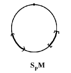
Figure 1. Subset of Unit Tangent Circle

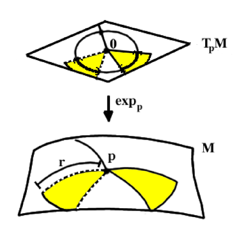
Figure 2. Illustration of Cones

The associated cones of radius $r$ in the tangent space and in the surface are illustrated in Figure 2.

In Chapter 9 of [Pet98] a volume comparison theorem for cones in manifolds is considered. We will need a version of this theorem that is valid for orbifolds. In order to state this theorem, we will use the following notation. We suppose $p$ is a point in an orbifold $O$ with fundamental coordinate chart $(U,\widetilde{U}/\Gamma,\pi)$. For $A\subset T_{p}O$, the set $\{\tilde{v}\in T_{\tilde{p}}\widetilde{U}:\pi_{*\tilde{p}}\tilde{v}\in A\}$ is denoted by $\widetilde{A}$.

Proposition 4.3.

(Volume comparison theorem for cones in orbifolds.) Let $O$ be a complete Riemannian orbifold with $\operatorname{Ric}(O)\geq(n-1)\kappa$, and take $p\in O$. If $\kappa>0$ suppose $r\leq\pi/\sqrt{\kappa}$, otherwise let $r$ be any non-negative real. Suppose $\mathfrak{a}$ is an open subset of $S_{p}O$ with boundary of measure zero, and $\overline{p}\in M^{n}_{\kappa}$. Let $I$ be an isometry from $S_{\tilde{p}}\widetilde{U}$ to $S_{\overline{p}}M^{n}_{\kappa}$, relative to the canonical metric on the unit sphere. Then,

$$\operatorname{Vol}B^{\mathfrak{a}}(p,r)\leq\frac{1}{|\Gamma_{p}|}\operatorname{Vol}B^{I(\tilde{\mathfrak{a}})}(\overline{p},r).$$

Proof.

First suppose that $p$ is a manifold point in $O$. Using the fact that $O-\Sigma_{O}$ is a convex manifold, and that $p$ has trivial isotropy, we conclude:

$$\operatorname{Vol}B^{\mathfrak{a}}(p,r)\leq\operatorname{Vol}B^{I(\mathfrak{a})}(\overline{p},r)=\frac{1}{|\Gamma_{p}|}\operatorname{Vol}B^{I(\tilde{\mathfrak{a}})}(\overline{p},r).$$

Now suppose $p$ is a singular point in $O$. Let $(U,\widetilde{U}/\Gamma,\pi)$ be a fundamental coordinate chart about $p$. Suppose $\tilde{p}\in\widetilde{U}$ projects to $p$, and lift $\mathfrak{a}$ to $\tilde{\mathfrak{a}}\subset S_{\tilde{p}}\widetilde{U}$.

Choose a vector $v\in\mathfrak{a}$ that points out of the singular set. Fix a lift $\tilde{v}$ of $v$ in $\tilde{\mathfrak{a}}$. Recall that the Dirichlet fundamental domain centered at $\tilde{v}$ of the action of $\Gamma_{*_{\tilde{p}}}$ on $S_{\tilde{p}}\widetilde{U}$ is the set $\{u\in S_{\tilde{p}}\widetilde{U}:d(u,\tilde{v})\leq d(u,\gamma_{*_{\tilde{p}}}\tilde{v})\ \text{for all}\ \gamma_{*_{\tilde{p}}}\in\Gamma_{*_{\tilde{p}}}\}$. Let $\tilde{\mathfrak{b}}$ denote the intersection of this Dirichlet fundamental domain with $\tilde{\mathfrak{a}}$. Let $\gamma_{\tilde{v}}:[0,\varepsilon)\rightarrow\widetilde{U}$ be a portion of the geodesic emanating from $\tilde{p}$ in the direction $\tilde{v}$. Let $\gamma_{v}$ be the image of $\gamma_{\tilde{v}}$ under $\pi$. Shrink $\varepsilon$ as needed to ensure that $\gamma_{v}([0,t])$ is minimizing for all $t\in[0,\varepsilon)$ and that $\varepsilon<r$.

The parallel transport map $P_{0,t}:T_{\tilde{p}}\widetilde{U}\rightarrow T_{\gamma_{\tilde{v}}(t)}\widetilde{U}$ is a vector space isometry. Let $\tilde{\mathfrak{b}}(t)$ be the subset $P_{0,t}(\tilde{\mathfrak{b}})\subset S_{\gamma_{\tilde{v}}(t)}\widetilde{U}$. Note here that $\tilde{\mathfrak{b}}(0)=P_{0,0}(\tilde{\mathfrak{b}})=\tilde{\mathfrak{b}}$. This process smoothly spreads $\tilde{\mathfrak{b}}$ along the spheres tangent to points on the geodesic $\gamma_{\tilde{v}}(t)$.

Using this, for $t\in(0,\varepsilon)$ we can specify a subset $\mathfrak{b}(t)$ of $S_{\gamma_{v(t)}}O$ by $\mathfrak{b}(t)=\pi_{*\gamma_{\tilde{v}}(t)}(\tilde{\mathfrak{b}}(t))$.

For $A\subset O$ let $\chi_{A}$ denote the characteristic function of $A$ given by:

$$\chi_{A}(x)=\begin{cases}1&x\in A\\ 0&x\in O-A\end{cases}.$$

We will show that as $t$ goes to zero in $[0,\varepsilon)$, the functions $\chi_{B^{\mathfrak{b}(t)}(\gamma_{v}(t),r-t)}\rightarrow\chi_{B^{\mathfrak{a}}(p,r)}$ pointwise a.e. To do this we need to check that points in the cone $B^{\mathfrak{a}}(p,r)$ also lie in nearby cones $B^{\mathfrak{b}(t)}(\gamma_{v}(t),r-t)$, and points outside of $B^{\mathfrak{a}}(p,r)$ also lie outside nearby cones $B^{\mathfrak{b}(t)}(\gamma_{v}(t),r-t)$. Because the property of being in a particular cone depends on distance and angle, we check each of these in the two cases.

Fix $x$ in the $r$-ball about $p$. Then, for this $x$, we can find a $\delta_{1}>0$ sufficiently small so that $x$ will be in the balls $B(\gamma_{v}(t),r-t)$ for all $t\in[0,\delta_{1})$.

Now consider the directions from points on $\gamma_{v}$ to $x$. Let $\sigma_{t}$ denote the geodesic from $\gamma_{v}(t)$ to $x$. The fact that $x$ lies in $B^{\mathfrak{a}}(p,r)$ implies that $\sigma_{0}^{\prime}(0)\in\mathfrak{a}$. Noting that $\mathfrak{a}=\mathfrak{b}$ is an open subset of $S_{p}O$, we can assume there is a small neighborhood $\mathfrak{c}$ about $\sigma_{0}^{\prime}(0)$ in $\mathfrak{b}$. By lifting and translating as above we have $\mathfrak{c}(t)\subset\mathfrak{b}(t)$ for $t\in(0,\varepsilon)$. By continuity, $\sigma_{t}^{\prime}(0)$ will remain in $\mathfrak{c}(t)$ for $t$ small, say for $t\in[0,\delta_{2})$. Thus $\sigma_{t}^{\prime}(0)$ will remain in $\mathfrak{b}(t)$ for $t\in[0,\delta_{2})$.

Set $\delta=\min\{\delta_{1},\delta_{2}\}$. The previous two paragraphs imply that $x$ lies in the cones $B^{\mathfrak{b}(t)}(\gamma_{v}(t),r-t)$ for $t\in[0,\delta)$.

Now suppose that $x$ lies outside of the cone $B^{\mathfrak{a}}(p,r)$. This means that either the distance between $p$ and $x$ is larger than $r$, or the direction from $p$ to $x$ lies outside of $\mathfrak{a}$. We need to confirm that in either of these cases, $x$ also lies outside of cones $B^{\mathfrak{b}(t)}(\gamma_{v}(t),r-t)$ for small $t$. Because the balls $B(\gamma_{v}(t),r-t)$ are contained in $B(p,r)$, it is clear that points lying outside of $B(p,r)$ are also outside of $B(\gamma_{v}(t),r-t)$ for $t\in[0,\varepsilon)$.

Suppose that $x$ fails to be in $B^{\mathfrak{a}}(p,r)$ because the direction from $p$ to $x$ is not in $\mathfrak{a}$. As before let $\sigma_{t}$ denote the geodesic from $\gamma_{v}(t)$ to $x$. That the direction from $p$ to $x$ lies outside of $\mathfrak{a}$ is written more precisely as $\sigma_{0}^{\prime}(0)\in S_{p}O-\mathfrak{a}$. Disregarding points on the boundary of $B^{\mathfrak{a}}(p,r)$, we can assume the slightly stronger statement that $\sigma_{0}^{\prime}(0)\in S_{p}O-\overline{\mathfrak{a}}$. Take a small neighborhood $\mathfrak{c}$ about $\sigma_{0}^{\prime}(0)$ in $S_{p}O-\overline{\mathfrak{a}}$. By continuity there is an $\eta>0$ such that $\sigma_{t}^{\prime}(0)$ lies outside of $\mathfrak{b}(t)$ for all $t\in[0,\eta)$. Thus $x$ lies outside of the cones $B^{\mathfrak{b}(t)}(\gamma_{v}(t),r-t)$ for $t\in[0,\eta)$ as desired.

We are now able to apply the Lebesgue Dominated Convergence Theorem to obtain,

$$\operatorname{Vol}B^{\mathfrak{b}(t)}(\gamma_{v}(t),r-t)=\int_{O-\Sigma_{O}}\chi_{B^{\mathfrak{b}(t)}(\gamma_{v}(t),r-t)}dV\stackrel{{\scriptstyle t\rightarrow 0}}{{\longrightarrow}}\int_{O-\Sigma_{O}}\chi_{B^{\mathfrak{a}}(p,r)}dV=\operatorname{Vol}B^{\mathfrak{a}}(p,r).$$

For $t\in(0,\varepsilon)$, each $\gamma_{v}(t)$ is a manifold point in $O$. Because the proposition holds for manifold points, we conclude that if $t\in(0,\varepsilon)$ then,

$$\operatorname{Vol}B^{\mathfrak{b}(t)}(\gamma_{v}(t),r)\leq\operatorname{Vol}B^{I(\mathfrak{b}(t))}(\overline{p},r).$$

Now on $(0,\varepsilon)$ we have $\mathfrak{b}(t)$ isometric to $\tilde{\mathfrak{b}}(t)$ via $\pi_{*\gamma_{\tilde{v}}(t)}$, and $\tilde{\mathfrak{b}}(t)$ is isometric to $\tilde{\mathfrak{b}}$ via $P_{0,t}$. Thus,

$$\operatorname{Vol}B^{\mathfrak{b}(t)}(\gamma_{v}(t),r)\leq\operatorname{Vol}B^{I(\tilde{\mathfrak{b}})}(\overline{p},r).$$

Taking the limit as $t\rightarrow 0$ in this inequality yields,

$$\operatorname{Vol}B^{\mathfrak{a}}(p,r)\leq\operatorname{Vol}B^{I(\tilde{\mathfrak{b}})}(\overline{p},r).$$

Finally because the translates of $\tilde{\mathfrak{b}}$ cover $\tilde{\mathfrak{a}}$ and overlap on a set of measure zero, we have,

$$\operatorname{Vol}B^{I(\tilde{\mathfrak{b}})}(\overline{p},r)=\frac{1}{|\Gamma_{p}|}\operatorname{Vol}B^{I(\tilde{\mathfrak{a}})}(\overline{p},r).$$

∎

We end this section with a version of Toponogov’s Theorem for orbifolds. In [Bor93] it is shown that orbifolds with sectional curvature bounded below by $\kappa\in\mathbf{R}$ have Toponogov curvature greater than or equal to $\kappa$ in the sense of length spaces. In particular, an orbifold with a lower bound $\kappa$ on sectional curvature is an Alexandrov space with curvature bounded below by $\kappa$.

The following proposition is proven in [Shi93].

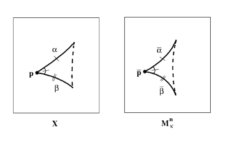
Figure 3. Hinges in Toponogov’s Theorem

Proposition 4.4.

Let $X$ be an Alexandrov space with curvature bounded below by $\kappa$. Let $\alpha:[0,a]\rightarrow X$ and $\beta:[0,b]\rightarrow X$ be geodesics with $\alpha(0)=\beta(0)=p$ (see Figure 3). Let $\overline{\alpha}$ and $\overline{\beta}$ be geodesics from point $\overline{p}$ in $M^{n}_{\kappa}$ with the same lengths as $\alpha$ and $\beta$, respectively, and with $\angle(\alpha^{\prime}(0),\beta^{\prime}(0))=\angle(\overline{\alpha}^{\prime}(0),\overline{\beta}^{\prime}(0))$. Then $d(\alpha(a),\beta(b))\leq d(\overline{\alpha}(a),\overline{\beta}(b))$.

We conclude that the hinge version of Toponogov’s Theorem is valid for orbifolds.

5. Spectral Geometry Background

To prove our two main theorems we will need to be able to convert spectral hypotheses into explicit bounds on geometry. This section provides background on the spectrum of the Laplacian for orbifolds, and establishes facts that will be needed to obtain a diameter bound in Section 6. Useful references for the material in this Section are [Cha84] and [Bér86].

In this section orbifolds are assumed to be compact and orientable. The inner product on $L^{2}(O)$ will be indicated with parentheses, $(\cdot,\cdot)$. For vector fields $X$ and $Y$ on an orbifold $O$, we will use $(X,Y)$ to denote the inner product $\int_{O}<X,Y>\ dV$.

Let $O$ be a Riemannian orbifold and let $f$ be a smooth function on $O$. The Laplacian $\Delta f$ of $f$ is given by the Laplacian of lifts of $f$ in the orbifold’s local coverings. More precisely, lift $f$ to $\tilde{f}=f\circ\pi$ via a coordinate chart $(U,\widetilde{U}/\Gamma,\pi)$. Let $g_{ij}$ denote the $\Gamma$-invariant metric on $\tilde{U}$ and $\rho$ = $\sqrt{\text{det}(g_{ij})}$ as in Section 3. On this local cover $\Delta\tilde{f}$ is given in the usual way,

$$\Delta\tilde{f}=\frac{1}{\rho}\sum_{i,j=1}^{n}\frac{\partial}{\partial\tilde{x}^{i}}(g^{ij}\frac{\partial f}{\partial\tilde{x}^{j}}\rho).$$

The study of the spectrum of the Laplacian begins with the problem of finding all of the Laplacian’s eigenvalues as it acts on $C^{\infty}(O)$. That is, we seek all numbers $\lambda$, with multiplicities, that solve $\Delta f=\lambda f$ for some nontrivial $f\in C^{\infty}(O)$.

The following theorem is proven in [Chi93].

Theorem 5.1.

Let $O$ be a Riemannian orbifold.

1. The set of eigenvalues $\lambda$ in $\Delta f=\lambda f$ consists of an infinite sequence $0\leq\overline{\lambda_{1}}<\overline{\lambda 2}<\overline{\lambda 3}<\dots\uparrow\infty$.

2. Each eigenvalue $\lambda_{i}$ has finite multiplicity. (Eigenvalues will henceforth be listed as $0\leq\lambda_{1}\leq\lambda_{2}\leq\lambda_{3}\dots\uparrow\infty$ with each eigenvalue repeated according to its multiplicity.)

3. There exists an orthonormal basis of $L^{2}(O)$ composed of smooth eigenfunctions $\varphi_{1},\varphi_{2},\varphi_{3}\dots$ where $\Delta\varphi_{i}=\lambda_{i}\varphi_{i}$.

The sequence $0\leq\lambda_{1}\leq\lambda_{2}\leq\lambda_{3}\dots\uparrow\infty$ in Theorem 5.1(2) is called the spectrum of the Laplacian on $O$. It will be denoted by $Spec(O)$.

The first Sobolev space of a Riemannian orbifold $O$ is obtained by completing $C^{\infty}(O)$ with respect to the norm associated to the following inner product,

$$(f,h)_{1}=(f,h)+(\nabla f,\nabla h).$$

We’ll denote the first Sobolev space by $\mathcal{H}(O)$, and the associated norm by $||\cdot||_{1}$. Note that,

$$C^{\infty}(O)\subset\mathcal{H}(O)\subset L^{2}(O).$$

Non-smooth elements $u$ of $\mathcal{H}(O)$ possess first derivatives in the distributional sense. In analogy with the gradient of a smooth function, these weak derivatives will be denoted by $\nabla u$. See [Far01] for information about general orbifold Sobolev spaces.

A useful tool in spectral geometry is the Rayleigh quotient. It is defined as follows.

Definition 5.2.

For $h\in\mathcal{H}(O)$ with $\int_{O}h^{2}dV\neq 0$ the Rayleigh quotient of $h$ is defined by,

$$R(h)=\frac{\int_{O}<\nabla h,\nabla h>dV}{\int_{O}h^{2}dV}.$$

The proof of Rayleigh’s Theorem for the closed eigenvalue problem extends from the manifold category to the orbifold category without difficulty.

Lemma 5.3.

(Rayleigh’s Theorem for Orbifolds) Let $O$ be a Riemannian orbifold with eigenvalue spectrum $0\leq\lambda_{1}\leq\lambda_{2}\leq\lambda_{3}\dots\uparrow\infty$.

1. Then for any $h\in\mathcal{H}(O)$, with $h\neq 0$, we have $R(h)\geq\lambda_{1}$ with equality if and only if $h$ is an eigenfunction of $\lambda_{1}$.

2. Suppose $\{\varphi_{1},\varphi_{2},\dots\}$ is a complete orthonormal basis of $L^{2}(O)$ with $\varphi_{i}$ an eigenfunction of $\lambda_{i}$, $i=1,2,3,\dots$. If $h\in\mathcal{H}(O)$ with $h\neq 0$ satisfies $(h,\varphi_{1})=(h,\varphi_{2})=\dots=(h,\varphi_{k-1})=0$, then $R(h)\geq\lambda_{k}$ with equality if and only if $h$ is an eigenfunction of $\lambda_{k}$.

In [Far01] it is shown that Weil’s asymptotic formula extends to the orbifold category as well.

Theorem 5.4.

(Weil’s asymptotic formula) Let $O$ be a Riemannian orbifold with eigenvalue spectrum $0\leq\lambda_{1}\leq\lambda_{2}\leq\lambda_{3}\dots\uparrow\infty$. Then for the function $N(\lambda)=\sum_{\lambda_{j}\leq\lambda}1$ we have

$$N(\lambda)\sim(\operatorname{Vol}B^{n}_{0}(1))(\operatorname{Vol}O)\frac{\lambda^{n/2}}{(2\pi)^{n}}$$

as $\lambda\uparrow+\infty$. Here $B^{n}_{0}(1)$ denotes the $n$-dimensional unit ball in Euclidean space.

Thus, as with the manifold case, the Laplace spectrum determines an orbifold’s dimension and volume.

6. Obtaining the Diameter Bound

By applying volume comparison tools in the spectral setting, we derive an upper diameter bound for an orbifold that relies on spectral information and the presence of a lower Ricci curvature bound. With the diameter bound established, an application of the Orbifold Relative Volume Comparison Theorem (Proposition 4.1) proves the first main theorem.

As in the preceding section, we assume that all orbifolds are compact and orientable. Also, we will let $R(\cdot)$ denote the Rayleigh quotient from Section 5, Definition 5.2.

For any open set $U$ in $O$, let $\mathcal{H}_{0}(U)$ denote the completion of $C^{\infty}_{0}(U)$ in $\mathcal{H}(U)$.

Definition 6.1.

Let $U$ be an arbitrary open set in a Riemannian orbifold $O$. The fundamental tone of $U$, denoted $\lambda^{*}(U)$ is defined by,

$$\lambda^{*}(U)=\inf\{R(f)\ :\;f\in\mathcal{H}_{0}(U),f\neq 0\}.$$

The following fact about the fundamental tone will be used in the proof of the orbifold version of Cheng’s Theorem. Its proof is identical to that of the manifold version.

Lemma 6.2.

Let $\{U_{\alpha}\}_{\alpha\in I}$ be a set of domains in a Riemannian orbifold $O$. Set $U=\bigcup_{\alpha}U_{\alpha}$. Then $\lambda^{*}(U)\leq\inf_{\alpha}\lambda^{*}(U_{\alpha})$.

In what follows let $M^{n}_{\kappa}$ denote the $n$-dimensional simply connected space form of constant curvature $\kappa$. Let $B^{n}_{\kappa}(r)$ denote the ball of radius $r$ in $M^{n}_{\kappa}$, and let $\lambda^{n}_{\kappa}(r)$ denote the lowest Dirichlet eigenvalue of $B^{n}_{\kappa}(r)$.

Proposition 6.3.

(Cheng’s Theorem for orbifolds.) Let $O$ be an $n$-dimensional Riemannian orbifold with Ricci curvature bounded below by $\kappa(n-1)$, $\kappa$ real. Then for any $r>0$ and $p\in O$ we have,

$$\lambda^{*}(B(p,r))\leq\lambda^{n}_{\kappa}(r).$$

Proof.

If $p$ is a manifold point in $O$, the manifold proof of Cheng’s Theorem carries over to orbifolds (see [Cha84]).

Now suppose $p$ is an arbitrary point in $O$, and take $\{p_{i}\}\subset(O-\Sigma_{O})$ such that $\{p_{i}\}\rightarrow p$. Consider the infinite collection of balls $\{B(p_{i},r-d(p_{i},p)\}_{i=1}^{\infty}$. Note in particular that $\bigcup_{i=1}^{\infty}B(p_{i},r-d(p,p_{i}))$ is equal to $B(p,r)$. By Lemma 6.2 we have

$$\lambda^{*}(B(p,r))\leq\inf_{i}\lambda^{*}(B(p_{i},r-d(p_{i},p))).$$

Since the $p_{i}$’s are manifold points we can invoke the previous case to obtain,

(1) $$\lambda^{*}(B(p,r))\leq\inf_{i}\lambda^{*}(B(p_{i},r-d(p_{i},p)))\leq\inf_{i}\lambda_{\kappa}^{n}(r-d(p_{i},p)).$$

Finally by domain monotonicity of eigenvalues we have,

(2) $$\inf_{i}\lambda^{n}_{\kappa}(r-d(p_{i},p))=\lambda^{n}_{\kappa}(r).$$

Combining lines 1 and 2 concludes the argument. ∎

We now adapt a method introduced in [BPP92] to the orbifold setting. This method uses spectral data about an orbifold, together with a lower Ricci curvature bound, to obtain an upper bound on the diameter of the orbifold. Recall that $\lambda^{n}_{\kappa}(r)$ denotes the lowest Dirichlet eigenvalue of $B^{n}_{\kappa}(r)$.

Proposition 6.4.

Let $O$ be a compact Riemannian orbifold with Ricci curvature bounded below by $\kappa(n-1)$, $\kappa$ real. Fix arbitrary constant $r$ greater than zero. Then the number of disjoint balls of radius $r$ that can be placed in $O$ is bounded above by a number that depends only on $\kappa$ and the number of eigenvalues of $O$ less than or equal to $\lambda_{\kappa}^{n}(r)$.

In particular the diameter of $O$ is bounded above by a number that depends only on $Spec(O)$, $\kappa$ and $r$.

Proof.

As before, write the eigenvalue spectrum of $O$ as $\lambda_{1}\leq\lambda_{2}\leq\lambda_{3}\leq\dots\uparrow\infty$. Choose $\varepsilon>0$ so that no eigenvalues of $O$ lie between $\lambda_{\kappa}^{n}(r)$ and $\lambda_{\kappa}^{n}(r)+\varepsilon$. Take a collection of $N(r)$ pairwise disjoint metric $r$-balls $B(p_{1},r)$, $B(p_{2},r)$, $\dots$, $B(p_{N(r)},r)$ in $O$. By Cheng’s Theorem (Proposition 6.3) we have for each $i$ a function $f^{i}\in\mathcal{H}_{0}(B(p_{i},r))$ such that $R(f^{i})\leq\lambda_{\kappa}^{n}(r)+\varepsilon$.

Because $\mathcal{H}_{0}(B(p_{i},r))$ is the closure of $C^{\infty}_{0}(B(p_{i},r))$ with respect to $||\cdot||_{1}$ we can find for each $i$ a sequence $\{h_{j}^{i}\}_{j=1}^{\infty}\subset C^{\infty}_{0}(B(p_{i},r))$ that converges to $f^{i}$. By the continuity of $R:\mathcal{H}(O)\rightarrow\mathbf{R}$ we know additionally that $R(h^{i}_{j})\rightarrow R(f^{i})$ as $j\rightarrow\infty$. In particular for $\varepsilon^{\prime}>0$ arbitrary we can choose integers $k(i)$ large enough that $|R(h^{i}_{k(i)})-R(f^{i})|<\varepsilon^{\prime}$ for each $i$.

Extend each $h^{i}_{k(i)}$ to all of $O$ by setting it equal to zero off of $B(p_{i},r)$. Now $(h^{i}_{k(i)},h^{j}_{k(j)})=0$ for $i\neq j$ as the supports of these functions are disjoint. To arrange that the collection $\{h^{i}_{k(i)}\}_{i=1}^{\infty}$ is orthonormal replace each $h^{i}_{k(i)}$ with $\overline{h}^{i}_{k(i)}=\frac{h^{i}_{k(i)}}{|h^{i}_{k(i)}|}$.

Pick $\varphi_{1},\varphi_{2},\dots,\varphi_{N(r)-1}\in L^{2}(O)$ which are orthonormal and which are eigenfunctions for $\lambda_{1},\lambda_{2},\dots,\lambda_{N(r)-1}$ respectively. There exist $\alpha_{1},\alpha_{2},\dots,\alpha_{N(r)}$, not all zero, such that,

$$\Sigma^{N(r)}_{l=1}\alpha_{l}(\overline{h}^{l}_{k(l)},\varphi_{m})=0,$$

for $m=1,2,\dots,N(r)-1$. Setting $\psi=\Sigma^{N(r)}_{l=1}\alpha_{l}\overline{h}_{k(l)}^{l}$, Rayleigh’s Theorem yields,

$$\lambda_{N(r)}|\psi|^{2} \leq(\nabla\psi,\nabla\psi)$$

$$=(\Sigma^{N(r)}_{l=1}\alpha_{l}\nabla\overline{h}_{k(l)}^{l},\Sigma^{N(r)}_{l=1}\alpha_{l}\nabla\overline{h}_{k(l)}^{l})$$

$$=\Sigma^{N(r)}_{l,s=1}\alpha_{l}\alpha_{s}(\nabla\overline{h}_{k(l)}^{l},\nabla\overline{h}_{k(s)}^{s})$$

$$=\Sigma^{N(r)}_{l=1}\alpha_{l}^{2}(\nabla\overline{h}_{k(l)}^{l},\nabla\overline{h}_{k(l)}^{l})$$

$$=\Sigma^{N(r)}_{l=1}\alpha_{l}^{2}\frac{(\nabla h_{k(l)}^{l},\nabla h_{k(l)}^{l})}{|h_{k(l)}^{l}|^{2}}$$

$$=\Sigma^{N(r)}_{l=1}\alpha_{l}^{2}R(h^{l}_{k(l)}).$$

Now observe that $|\psi|^{2}=\Sigma^{N(r)}_{l=1}\alpha_{l}^{2}$. The calculation above then implies,

$$\lambda_{N(r)}\Sigma^{N(r)}_{l=1}\alpha_{l}^{2}\leq\Sigma^{N(r)}_{l=1}\alpha_{l}^{2}R(h^{l}_{k(l)}).$$

By our choice of $k(l)$ we have,

$$\lambda_{N(r)}\Sigma^{N(r)}_{l=1}\alpha_{l}^{2}\leq\Sigma^{N(r)}_{l=1}\alpha_{l}^{2}(R(f^{l})+\varepsilon^{\prime}).$$

And our choice of $f^{l}$ gives,

$$\lambda_{N(r)}\Sigma^{N(r)}_{l=1}\alpha_{l}^{2}\leq\Sigma^{N(r)}_{l=1}\alpha_{l}^{2}(\lambda^{n}_{\kappa}(r)+\varepsilon+\varepsilon^{\prime}).$$

Since we know at least one $\alpha_{l}$ is nonzero, we can divide both sides by $\Sigma^{N(r)}_{l=1}\alpha_{l}^{2}$ to obtain $\lambda_{N(r)}\leq\lambda^{n}_{\kappa}(r)+\varepsilon+\varepsilon^{\prime}$. Letting $\varepsilon^{\prime}$ go to zero simplifies the right hand side further and we have,

$$\lambda_{N(r)}\leq\lambda^{n}_{\kappa}(r)+\varepsilon.$$

Because $\varepsilon$ was chosen so that no eigenvalues of $O$ appeared in $(\lambda^{n}_{\kappa}(r),\lambda^{n}_{\kappa}(r)+\varepsilon)$, we can conclude that $\lambda_{N(r)}\leq\lambda^{n}_{\kappa}(r)$.

We now obtain the diameter bound. Let $\rho$ be the largest number so that $\lambda_{\rho}(O)\leq\lambda^{n}_{\kappa}(r)$. Then $\lambda_{N(r)}\leq\lambda^{n}_{\kappa}(r)$ implies that $N(r)\leq\rho$. Thus the number of disjoint $r$-balls is bounded by the spectral invariant $\rho$. Now an orbifold of diameter $d$ contains at least $[d/2r]$ disjoint $r$-balls, where $[\cdot]$ denotes the greatest integer function. Thus $d$ must satisfy $[d/2r]\leq\rho$. This gives an upper bound on the diameter of $O$ which depends only on $r$, $\kappa$ and $Spec(O)$. ∎

We are now prepared to prove our first main result.

Main Theorem 1: Let $\mathcal{S}$ be a collection of isospectral Riemannian orbifolds that share a uniform lower bound $\kappa(n-1)$, $\kappa$ real, on Ricci curvature. Then there are only finitely many possible isotropy types, up to isomorphism, for points in an orbifold in $\mathcal{S}$.

Proof.

It is shown above that isospectral families of orbifolds which share a uniform lower Ricci curvature bound also share an upper diameter bound. Let $D>0$ be the upper bound for the diameter of orbifolds in $\mathcal{S}$. By Weil’s asymptotic formula, the isospectrality of the orbifolds in $\mathcal{S}$ implies that they all have the same dimension $n$ and the same volume $v>0$.

Let $O$ be an orbifold in $\mathcal{S}$ and take $p\in O$. As before let $B^{n}_{\kappa}(r)$ denote the $r$-ball in the simply connected, $n$-dimensional space form of constant curvature $\kappa$. For $R>r\geq 0$ we have by Proposition 4.1,

$$\frac{\operatorname{Vol}B(p,r)}{B^{n}_{\kappa}(r)}\geq\frac{\operatorname{Vol}B(p,R)}{B^{n}_{\kappa}(R)}.$$

Letting $R=D$ in this inequality gives,

$$\frac{\operatorname{Vol}B(p,r)}{B^{n}_{\kappa}(r)}\geq\frac{\operatorname{Vol}O}{B^{n}_{\kappa}(D)}=\frac{v}{B^{n}_{\kappa}(D)}.$$

Again applying Proposition 4.1 we take the limit as $r\rightarrow 0$ to obtain,

$$\frac{1}{|\Gamma_{p}|}=\lim_{r\rightarrow 0}\frac{\operatorname{Vol}B(p,r)}{B^{n}_{\kappa}(r)}\geq\frac{v}{B^{n}_{\kappa}(D)}.$$

We conclude for any point in any orbifold in $\mathcal{S}$, the isotropy group of that point has order less than or equal to the universal constant $B^{n}_{\kappa}(D)/v$. This implies that the isotropy group of the point can have one of only finitely many possible isomorphism types. ∎

Consider the collection of all closed, connected Riemannian $n$-orbifolds with a lower bound $\kappa(n-1)$, $\kappa$ real, on Ricci curvature, a lower bound $v>0$ on volume, and an upper bound $D>0$ on diameter. A similar argument to the one above shows that there are only finitely many possible isotropy types for points in an orbifold in this collection.

7. Spectral Bounds on Isolated Singular Points

This section begins by extending a technical result from [GP88] to the orbifold setting. Assume the orbifolds under consideration are compact and orientable. As in Section 4, we will use $B^{\mathfrak{a}}(p,r)$ to denote the cone of radius $r$ at point $p$ in an orbifold with directions given by $\mathfrak{a}\in S_{p}O$. Following [GP88] we will use the symbol $\mathcal{O}^{\cdot,D,\cdot}_{\kappa,\cdot,v}(n)$ to denote the collection of all closed, connected $n$-dimensional Riemannian orbifolds with volume bounded below by $v>0$, sectional curvature bounded below by $\kappa\in\mathbf{R}$, and with diameter bounded above by $D>0$. The subcollection of orbifolds in $\mathcal{O}^{\cdot,D,\cdot}_{\kappa,\cdot,v}(n)$ with only isolated singularities will be denoted by $isol\mathcal{O}^{\cdot,D,\cdot}_{\kappa,\cdot,v}(n)$.

Suppose $O$ is a complete orbifold and $K$ is a compact subset of $O$. Let $\mathfrak{d}_{\scriptscriptstyle{pK}}$ denote the set of unit tangent vectors at $p$ which are the velocity vectors of segments running from $p$ to $K$. The set $\mathfrak{d}_{\scriptscriptstyle{pK}}$ is called the set of directions from $p$ to $K$.

For subset $\mathfrak{a}$ of the unit $n$-sphere, $S^{n}$, we write,

$$\mathfrak{a}(\theta) =\{v\in S^{n}:\angle(\mathfrak{a},v)<\theta\}$$

$$\mathfrak{a}^{\prime}(\theta) =\{v\in S^{n}:\angle(\mathfrak{a},v)\geq\theta\}.$$

Lemma 7.1.

Suppose for some $\alpha\in[0,\frac{\pi}{2}]$, a finite subset $A$ of $S^{n}$ satisfies,

$$\overline{A\bigl{(}\frac{\pi}{2}+\alpha\bigr{)}}=S^{n}.$$

Let $\tilde{\mathfrak{a}}_{\alpha}\subset S^{n}$ consist of two vectors situated at an angle of $\pi-2\alpha$ from each other. Then, using the standard volume on $S^{n}$, we have:

$$\text{Vol }A(\theta)\geq\text{Vol }\tilde{\mathfrak{a}}_{\alpha}(\theta)$$

for all $\theta$ greater than or equal to zero.

Proof.

See the appendix in [GP88]. ∎

Lemma 7.2.

Let $O\in isol\mathcal{O}^{\cdot,D,\cdot}_{\kappa,\cdot,v}(n)$ and $p,q\in O$. There exist $\alpha\in(0,\frac{\pi}{2})$ and $r>0$ such that if,

$$\mathfrak{d}_{pq}(\frac{\pi}{2}+\alpha)=S_{p}O,\ \text{and}\ \mathfrak{d}_{qp}(\frac{\pi}{2}+\alpha)=S_{q}O,$$

then $d(p,q)\geq r$. The constants $\alpha$ and $r$ depend only on $\kappa$, $D$, $v$ and $n$.

A remark on the positive curvature case is necessary before proving this lemma. If $\kappa>0$ then the Bonnet-Myers Theorem implies that for $O\in\mathcal{O}^{\cdot,D,\cdot}_{\kappa,\cdot,v}(n)$, the manifold $O-\Sigma_{O}$ has diameter less than or equal to $\pi/\sqrt{\kappa}$. Thus $O$ itself satisfies this diameter bound. So in the positive curvature case we can assume $D\leq\pi/\sqrt{\kappa}$. In particular orbifolds in $\mathcal{O}^{\cdot,D,\cdot}_{\kappa,\cdot,v}(n)$ satisfy the hypotheses of the Volume Comparison Theorem for cones in orbifolds (Proposition 4.3), which will be used below.

Proof.

(Lemma 7.2) For a parameter $\alpha\in(0,\frac{\pi}{2})$ let $\tilde{\mathfrak{a}}$ be a subset of $S^{n-1}$ consisting of two vectors, $v$ and $w$, for which $\angle(v,w)=\pi-2\alpha$. Let $\bar{p}$ be an element of $M^{n}_{\kappa}$, the simply connected complete $n$-dimensional space form of constant curvature $\kappa$. We specify $\alpha$ by choosing it as an element of $(0,\frac{\pi}{2})$ such that:

$$\operatorname{Vol}B^{\tilde{\mathfrak{a}}^{\prime}(\frac{\pi}{2}-\alpha)}(\bar{p},D)<\frac{v}{6}.$$

Suppose we have points $p$ and $q$ in $O$ for which,

$$\mathfrak{d}_{pq}(\frac{\pi}{2}+\alpha)=S_{p}O,\ \text{and}\ \ \mathfrak{d}_{qp}(\frac{\pi}{2}+\alpha)=S_{q}O.$$

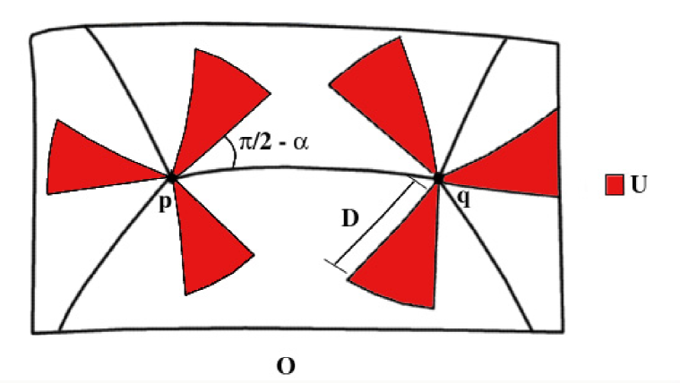
Figure 4. The Set $U$

Now, $S_{p}O$ and $S_{q}O$ are compact so we can take finite subsets $\mathfrak{d}_{p}$ and $\mathfrak{d}_{q}$ of ${\mathfrak{d}}_{pq}$ and ${\mathfrak{d}}_{qp}$, respectively, so that

$$\mathfrak{d}_{p}(\frac{\pi}{2}+\alpha)=S_{p}O,\ \text{and}\ \ \mathfrak{d}_{q}(\frac{\pi}{2}+\alpha)=S_{q}O$$

as well. Lifting these sets gives,

$$\tilde{\mathfrak{d}}_{p}(\frac{\pi}{2}+\alpha)=S_{\tilde{p}}\widetilde{U}_{p},\ \text{and}\ \ \tilde{\mathfrak{d}}_{q}(\frac{\pi}{2}+\alpha)=S_{\tilde{q}}\widetilde{U}_{q}.$$

Because of this we can use Lemma 7.1 to conclude that,

$$\operatorname{Vol}(\tilde{\mathfrak{d}}_{p}^{\prime}(\frac{\pi}{2}-\alpha))\leq\operatorname{Vol}(\tilde{\mathfrak{a}}^{\prime}(\frac{\pi}{2}-\alpha)),\ \text{and}\ \ \operatorname{Vol}(\tilde{\mathfrak{d}}_{q}^{\prime}(\frac{\pi}{2}-\alpha))\leq\operatorname{Vol}(\tilde{\mathfrak{a}}^{\prime}(\frac{\pi}{2}-\alpha)).$$

Let $U$ be the subset of $O$ given by,

$$U =B^{\operatorname{int}(\mathfrak{d}_{p}^{\prime}(\frac{\pi}{2}-\alpha))}(p,D)\cup B^{\operatorname{int}(\mathfrak{d}_{q}^{\prime}(\frac{\pi}{2}-\alpha))}(q,D),$$

where $\operatorname{int}(\mathfrak{d}_{p}^{\prime}(\frac{\pi}{2}-\alpha))$ denotes the interior of $\mathfrak{d}_{p}^{\prime}(\frac{\pi}{2}-\alpha)$, and $\operatorname{int}(\mathfrak{d}_{q}^{\prime}(\frac{\pi}{2}-\alpha))$ denotes the interior of $\mathfrak{d}_{q}^{\prime}(\frac{\pi}{2}-\alpha)$. A sketch of the set $U$ is given in Figure 4. The lines emanating from $p$ and $q$ indicate the segments between these points. The shaded regions are the cones that form $U$.

Let $I:S_{\tilde{p}}\widetilde{U}_{p}\rightarrow S_{\overline{p}}M^{n}_{\kappa}$ and $J:S_{\tilde{q}}\widetilde{U}_{q}\rightarrow S_{\overline{p}}M^{n}_{\kappa}$ be linear isometries. Then using Proposition 4.3 we have that $\operatorname{Vol}(U)<v/3$, as:

$$\operatorname{Vol}U \leq\operatorname{Vol}B^{\operatorname{int}(\mathfrak{d}_{p}^{\prime}(\frac{\pi}{2}-\alpha))}(p,D)+\operatorname{Vol}B^{\operatorname{int}(\mathfrak{d}_{q}^{\prime}(\frac{\pi}{2}-\alpha))}(q,D)$$

$$\leq\operatorname{Vol}B^{I(\operatorname{int}(\tilde{\mathfrak{d}}_{p}^{\prime}(\frac{\pi}{2}-\alpha)))}(\overline{p},D)+\operatorname{Vol}B^{J(\operatorname{int}(\tilde{\mathfrak{d}}_{q}^{\prime}(\frac{\pi}{2}-\alpha)))}(\overline{q},D)$$

$$=\operatorname{Vol}\operatorname{exp}_{\bar{p}}[0,D]I(\operatorname{int}(\tilde{\mathfrak{d}}_{p}^{\prime}(\frac{\pi}{2}-\alpha)))+\operatorname{Vol}\operatorname{exp}_{\bar{q}}[0,D]J(\operatorname{int}(\tilde{\mathfrak{d}}_{q}^{\prime}(\frac{\pi}{2}-\alpha)))$$

$$\leq\operatorname{Vol}\operatorname{exp}_{\bar{p}}[0,D]I(\tilde{\mathfrak{d}}_{p}^{\prime}(\frac{\pi}{2}-\alpha))+\operatorname{Vol}\operatorname{exp}_{\bar{q}}[0,D]J(\tilde{\mathfrak{d}}_{q}^{\prime}(\frac{\pi}{2}-\alpha))$$

$$\leq 2\operatorname{Vol}\operatorname{exp}_{\bar{p}}[0,D]\tilde{\mathfrak{a}}^{\prime}(\frac{\pi}{2}-\alpha)$$

$$<\frac{v}{3}.$$

We are ready to specify the constant $r$ required by the statement of the Lemma. First choose $l>0$ so that $\operatorname{Vol}B^{n}_{\kappa}(l)<v/3$ in $M^{n}_{k}$. Note that the Orbifold Relative Volume Comparison Theorem (Proposition 4.1) implies,

$$\operatorname{Vol}(B(p,l))<\frac{v}{3},\ \text{and}\ \ \operatorname{Vol}(B(q,l))<\frac{v}{3}.$$

Let $(c_{1};c_{2};c_{3})$ denote a geodesic triangle in $M^{n}_{\kappa}$ with sides $c_{1}$, $c_{2}$ and $c_{3}$. In triangle $(c_{1};c_{2};c_{3})$ the angle opposite side $c_{i}$ will be denoted by $\theta_{i}$. For the $\alpha\in(0,\frac{\pi}{2})$ and $l>0$ determined above, there exists an $r>0$ such that for all geodesic triangles $(c_{1};c_{2};c_{3})$ in $M^{n}_{\kappa}$ with $\theta_{1}\leq\frac{\pi}{2}-\alpha$, $L(c_{3})\geq l$ and $L(c_{2})<r<l$, we also have $L(c_{1})<L(c_{3})$.

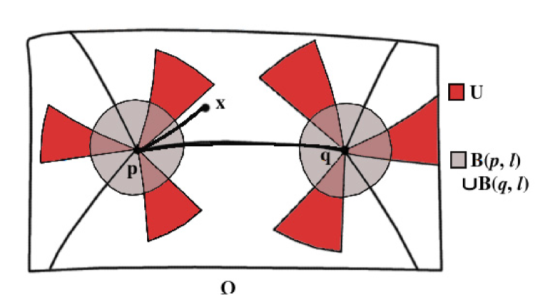
Figure 5. Hinge in $O$

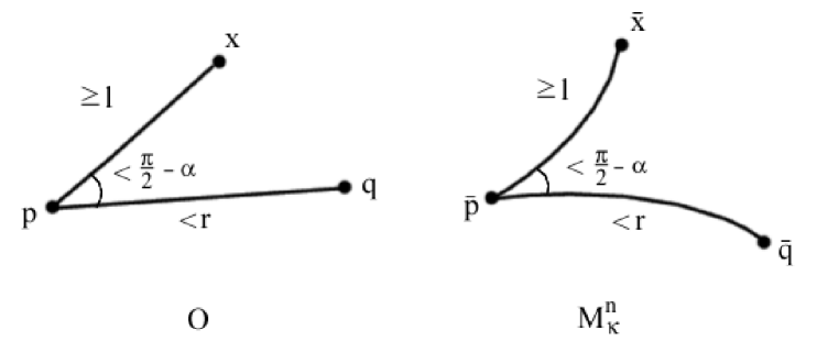
Figure 6. Hinge in $O$; Comparison Hinge in $M^{n}_{\kappa}$

We finish the proof by nested contradiction arguments. That is, we will show that if $p$ and $q$ satisfy the hypotheses of the Lemma, and $d(p,q)<r$, then the sets $U$, $B(p,l)$ and $B(q,l)$ cover $O$. However if these sets cover $O$ we have,

$$v\leq\operatorname{Vol}(O)\leq\operatorname{Vol}(U)+\operatorname{Vol}(B(p,l))+\operatorname{Vol}(B(q,l))<v.$$

Since this is a contradiction, once we show that $U$, $B(p,l)$, and $B(q,l)$ cover $O$ we can conclude that $d(p,q)\geq r$.

To show that $U$, $B(p,l)$, and $B(q,l)$ cover $O$ we argue again by contradiction. Suppose they fail to cover and we can find a point $x$ in $O-(U\cup B(p,l)\cup B(q,l))$. Set up a hinge with angle at $p$ terminating at $x$ and $q$ so that the leg of the hinge from $p$ to $q$ is a segment, and so that the hinge angle is less than $\frac{\pi}{2}-\alpha$. Figure 5 gives a sketch of this hinge in $O$. Using Toponogov’s Theorem for hinges in orbifolds, form a comparison hinge in $M^{n}_{\kappa}$ with angle at $\bar{p}$ terminating at $\bar{x}$ and $\bar{q}$. Figure 6 illustrates both the original hinge in $O$ and the comparison hinge in $M^{n}_{\kappa}$.

By Toponogov’s Theorem we know $d(x,q)\leq d(\bar{x},\bar{q})$. In addition our setup implies that $d(\bar{p},\bar{q})<r$, $d(\overline{p},\bar{x})\geq l$, and the angle formed by the comparison hinge is less than $\frac{\pi}{2}-\alpha$. So by our choice of $r$ we have $d(\bar{x},\bar{q})<d(\bar{x},\bar{p})$. Putting these observations together yields,

$$d(x,q)\leq d(\bar{x},\bar{q})<d(\bar{x},\bar{p})=d(x,p),$$

thus $d(x,q)<d(x,p)$. A similar argument based at $q$ yields the contradictory statement $d(x,p)<d(x,q)$, completing the proof. ∎

We now use Lemma 7.2 to bound the number of singular points that can appear in an orbifold in $isol\mathcal{O}^{\cdot,D,\cdot}_{\kappa,\cdot,v}(n)$. This in turn will lead to our second main theorem.

Fix $\varepsilon>0$. A minimal $\varepsilon$-net in a compact, connected metric space $X$ is an ordered set of points $p_{1},p_{2},\dots,p_{N}$ with the following two properties. First, the open balls $B(p_{i},\varepsilon)$, $i=1,2,\dots,N$, cover $X$. Second, the open balls $B(p_{i},\varepsilon/2)$, $i=1,2,\dots,N$ are disjoint. The fact that for any $\varepsilon>0$ we can find a minimal $\varepsilon$-net in $X$ is well known.

Proposition 7.3.

There is a positive integer $C(D,v,\kappa,n)$ for which no orbifold $O$ in the family $isol\mathcal{O}^{\cdot,D,\cdot}_{\kappa,\cdot,v}(n)$ has more than $C$ singular points.

Proof.

Suppose $O\in isol\mathcal{O}^{\cdot,D,\cdot}_{\kappa,\cdot,v}(n)$, and let $\alpha$ and $r$ be as in Lemma 7.2. Take $p\in\Sigma_{O}$ and let $(U,\widetilde{U}/\Gamma_{p},\pi)$ be a fundamental coordinate chart about $p$. Also, let $\tilde{p}$ denote the point in $\widetilde{U}$ which projects to $p$ under $\pi$. The set of lifts of a vector $v\in S_{p}O$ is the orbit $\Gamma_{p*}\tilde{v}$ of any vector $\tilde{v}\in S_{\tilde{p}}\widetilde{U}$ for which $\pi_{*_{\tilde{p}}}\tilde{v}=v$. We will first show that $\Gamma_{p*}\tilde{v}$ does not lie in any open hemisphere of $S_{\tilde{p}}\widetilde{U}$. With this established we can then appeal to Lemma 7.2 to conclude that the distance between two singular points in $O$ will always be greater than $r$. This in turn will be used to obtain the universal upper bound on the number of singular points in $O$.

Because $p$ is an isolated singularity, elements of $\Gamma_{p*}$ act on $S_{\tilde{p}}\widetilde{U}$ without fixed points. Thus the possible quotients $S_{\tilde{p}}\widetilde{U}/\Gamma_{p*}$ are actually all spherical space forms. Spherical space forms obtained as quotients of the sphere by finite groups of orthogonal transformations are well understood. See [Wol74] for example. In even dimensions the only non-trivial quotient is projective space, obtained as the quotient of $S^{2m}$ by the antipodal map. Since the orbits under the antipodal map consist of pairs of antipodal points, its clear that no orbit is contained in an open hemisphere.

Odd-dimensional spherical space forms, however, can arise in many ways. In this situation it will suffice to consider only those that are quotients of an odd dimensional sphere by the action of a cyclic group. This is because if we take an element $\gamma_{*_{\tilde{p}}}\in\Gamma_{p*}$ of order $l$, to show $\Gamma_{p*}\tilde{v}$ is not contained in an open hemisphere it suffices to show that $\{\tilde{v},\gamma_{*_{\tilde{p}}}\tilde{v},\gamma_{*_{\tilde{p}}}^{2}\tilde{v},\dots,\gamma_{*_{\tilde{p}}}^{l-1}\tilde{v}\}$ is not contained in any open hemisphere.

Suppose $\Gamma\leq O(2m)$ is cyclic and generated by $\gamma\in\Gamma$ of order $l$. Viewing $\mathbf{R}^{2m}$ as $\mathbf{C}^{m}$, element $\gamma$ can be expressed as:

$\begin{bmatrix}e^{2\pi i/l}&0&0&\dots&0\\ 0&e^{2\pi ia_{1}/l}&0&\dots&0\\ 0&0&e^{2\pi ia_{2}/l}&\dots&0\\ \vdots&\vdots&\vdots&\ddots&\vdots\\ 0&0&0&\dots&e^{2\pi ia_{m-1}/l}\\ \end{bmatrix}$

for $a_{1},a_{2},\dots,a_{m-1}\in\mathbf{R}$ each relatively prime to $l$. Thus the orbit of a vector $z=(z_{1},z_{2},\dots,z_{m})\in S^{2m-1}$ has the following form:

$$\{(e^{2\pi i/l}z_{1},e^{2\pi ia_{1}/l}z_{2},\dots,e^{2\pi ia_{m-1}/l}z_{m}), (e^{2\cdot 2\pi i/l}z_{1},e^{2\cdot 2\pi ia_{1}/l}z_{2},\dots,e^{2\cdot 2\pi ia_{m-1}/l}z_{m}),\dots,$$

$$(e^{2(l-1)\pi i/l}z_{1},e^{2(l-1)\pi ia_{1}/l}z_{2},\dots,e^{2(l-1)\pi ia_{m-1}/l}z_{m})\}.$$

If we sum together all of the orbits of $z$ under $\gamma$ we get the following vector in $\mathbf{R}^{2m}$:

(3) $$(\Sigma^{l-1}_{k=0}e^{2\pi ki/l}z_{1},\Sigma^{l-1}_{k=0}e^{2\pi ia_{1}k/l}z_{2},\dots,\Sigma^{l-1}_{k=0}e^{2\pi ia_{m-1}k/l}z_{m}).$$

By showing that this vector is actually the zero vector we will be able to conclude that $\{z,\gamma z,\gamma^{2}z,\dots,\gamma^{l-1}z\}$ does not lie in any open hemisphere.

To see that the vector in line 3 is the zero vector consider the $s^{th}$ entry,

$$\Sigma^{l-1}_{k=0}e^{2\pi ia_{s-1}k/l}z_{s}.$$

Since $a_{s-1}$ and $l$ are relatively prime, the set $\{e^{2\pi ia_{s-1}k/l}\}^{l-1}_{k=0}$ consists of $l^{\rm th}$ roots of unity. Because the sum of the $l^{\rm th}$ roots of unity is zero, we can conclude that this entry vanishes.

Now consider points $p$ and $q$ in the singular set of $O$. Because $O$ is complete we know that $p$ and $q$ are joined by at least one segment. Thus the set of directions from $p$ to $q$ contains at least one vector, namely the initial vector $v$ of the segment from $p$ to $q$. Moreover $\mathfrak{d}_{pq}(\frac{\pi}{2}+\alpha)=S_{p}O$. For if this were not the case we could find $w\in S_{p}O$ with $\angle(v,w)\geq\frac{\pi}{2}+\alpha$. However, this implies that if we let $\tilde{w}$ be a fixed lift of $w$ in the covering sphere $S_{\tilde{p}}\widetilde{U}$, then the orbit of a lift of $v$ is going to remain within the open hemisphere about $-\tilde{w}$. This contradicts our conclusions above. A similar argument shows that $\mathfrak{d}_{qp}(\frac{\pi}{2}+\alpha)=S_{q}O$. Thus by Lemma 7.2 we know that $d(p,q)\geq r$.

The proof concludes with a volume comparison argument. Let $\{x_{1},x_{2},\dots,x_{N}\}$ be a minimal $(r/2)$-net in $O$. Recall that for $p\in O$ and $S\geq s\geq 0$, Proposition 4.1 gives,

(4) $$\frac{\operatorname{Vol}B^{n}_{\kappa}(s)}{\operatorname{Vol}B^{n}_{\kappa}(S)}\leq\frac{\operatorname{Vol}B(p,s)}{\operatorname{Vol}B(p,S)}.$$

Without loss of generality suppose that $B(x_{1},r/4)$ is the minimal volume $(r/4)$-ball in our net. Then using the fact that the $(r/4)$-balls are disjoint we have,

$$N\operatorname{Vol}B(x_{1},r/4)\leq\Sigma_{i=1}^{N}\operatorname{Vol}B(x_{i},r/4)\leq\operatorname{Vol}O.$$

Thus $\operatorname{Vol}B(x_{1},r/4)\leq\operatorname{Vol}O/N$.

Now apply line 4 to balls about $x_{1}$ with $s=r/4$ and $S=D$. This yields,

(5) $$\frac{\operatorname{Vol}B^{n}_{\kappa}(r/4)}{\operatorname{Vol}B^{n}_{\kappa}(D)}\leq\frac{\operatorname{Vol}B(x_{1},r/4)}{\operatorname{Vol}B(x_{1},D)}.$$

Using $\operatorname{Vol}B(x_{1},D)=\operatorname{Vol}O$ and $\operatorname{Vol}B(x_{1},r/4)\leq\operatorname{Vol}O/N$ we find that line 5 becomes,

$$\frac{\operatorname{Vol}B^{n}_{\kappa}(r/4)}{\operatorname{Vol}B^{n}_{\kappa}(D)}\leq\frac{1}{N}.$$

Thus we see that the number of elements in our minimal $(r/2)$-net is bounded above by the universal constant $\operatorname{Vol}B^{n}_{\kappa}(D)/\operatorname{Vol}B^{n}_{\kappa}(r/4)$.

The singular points are all at least $r$-apart from each other, so there can be at most one singular point per $(r/2)$-ball in our net. Thus the bound on the number of elements in our net is also a bound on the number of singular points in $O$. ∎

Our second main result is a corollary to this proposition.

Main Theorem 2: Let $isol\mathcal{S}$ be a collection of isospectral Riemannian orbifolds with only isolated singularities that share a uniform lower bound $\kappa\in\mathbf{R}$ on sectional curvature. Then there is an upper bound on the number of singular points in any orbifold, $O$, in $isol\mathcal{S}$ depending only on $Spec(O)$ and $\kappa$.

Proof.

The argument begins in the same manner as that in the proof of Main theorem 1. Because these orbifolds are isospectral, and satisfy a lower bound on sectional curvature, we can conclude that they also share an upper diameter bound. By Weil’s asymptotic formula, we know that all orbifolds in $isol\mathcal{S}$ have the same volume and dimension. Therefore the family $isol\mathcal{S}$ satisfies the hypotheses of Proposition 7.3 and the theorem follows. ∎

References

- [Bér86] Pierre H. Bérard. Spectral geometry: direct and inverse problems. Springer-Verlag, Berlin, 1986. With appendixes by Gérard Besson, and by Bérard and Marcel Berger.
- [Bor93] Joseph E. Borzellino. Orbifolds of maximal diameter. Indiana Univ. Math. J., 42(1):37–53, 1993.
- [BPP92] Robert Brooks, Peter Perry, and Peter Petersen, V. Compactness and finiteness theorems for isospectral manifolds. J. Reine Angew. Math., 426:67–89, 1992.
- [Cha84] Isaac Chavel. Eigenvalues in Riemannian geometry. Academic Press Inc., Orlando, FL, 1984. Including a chapter by Burton Randol, With an appendix by Jozef Dodziuk.
- [Chi93] Yuan-Jen Chiang. Spectral geometry of -manifolds and its application to harmonic maps. In Differential geometry: partial differential equations on manifolds (Los Angeles, CA, 1990), pages 93–99. Amer. Math. Soc., Providence, RI, 1993.
- [Far01] Carla Farsi. Orbifold spectral theory. Rocky Mountain J. Math., 31(1):215–235, 2001.
- [GP88] Karsten Grove and Peter Petersen, V. Bounding homotopy types by geometry. Ann. of Math. (2), 128(1):195–206, 1988.
- [Gro99] Misha Gromov. Metric structures for Riemannian and non-Riemannian spaces. Birkhäuser Boston Inc., Boston, MA, 1999. Based on the 1981 French original [MR 85e:53051], With appendices by M. Katz, P. Pansu and S. Semmes, Translated from the French by Sean Michael Bates.
- [Pet98] Peter Petersen. Riemannian geometry. Springer-Verlag, New York, 1998.
- [Sat56] I. Satake. On a generalization of the notion of manifold. Proc. Nat. Acad. Sci. U.S.A., 42:359–363, 1956.
- [Sat57] Ichirô Satake. The Gauss-Bonnet theorem for -manifolds. J. Math. Soc. Japan, 9:464–492, 1957.
- [Shi93] Katsuhiro Shiohama. An introduction to the geometry of Alexandrov spaces. Seoul National University Research Institute of Mathematics Global Analysis Research Center, Seoul, 1993.
- [Thu78] William Thurston. The Geometry and Topology of 3-Manifolds. Lecture Notes, Princeton University Math. Dept., 1978.
- [Wol74] Joseph A. Wolf. Spaces of constant curvature. Publish or Perish Inc., Boston, Mass., third edition, 1974.