The Regge symmetry is a scissors congruencein hyperbolic space

Abstract

We give a constructive proof that the Regge symmetry is a scissors congruence in hyperbolic space. The main tool is Leibon’s construction for computing the volume of a general hyperbolic tetrahedron. The proof consists of identifying the key elements in Leibon’s construction and permuting them.

51M10 51M20

ATG Volume 3 (2003) 1–31Published: 24 January 2002

Abstract

AMS Classification;

Keywords

1 Introduction

The Regge symmetries are a family of involutive linear transformations on the six edges of a tetrahedron. They are defined as follows.

Definition 1.1.

Let $T(A,B,C,A^{\prime},B^{\prime},C^{\prime})$ denote a tetrahedron as shown in Figure 1. Define

$$R_{a}(T(A,B,C,A^{\prime},B^{\prime},C^{\prime}))=T(A,s_{a}-B,s_{a}-C,A^{\prime},s_{a}-B^{\prime},s_{a}-C^{\prime}),$$ (1)

where $s_{a}=(B+C+B^{\prime}+C^{\prime})/2$. Similarly, define

$$R_{b}(T(A,B,C,A^{\prime},B^{\prime},C^{\prime}))=T(s_{b}-A,B,s_{b}-C,s_{b}-A^{\prime},B^{\prime},s_{b}-C^{\prime}),$$ (2)

and

$$R_{c}(T(A,B,C,A^{\prime},B^{\prime},C^{\prime}))=T(s_{c}-A,s_{c}-B,C,s_{c}-A^{\prime},s_{c}-B^{\prime},C^{\prime}),$$ (3)

where $s_{b}=(A+C+A^{\prime}+C^{\prime})/2$ and $s_{c}=(A+B+A^{\prime}+B^{\prime})/2$. Then $R_{a}$, $R_{b}$, and $R_{c}$ generate the family of Regge symmetries of $T(A,B,C,A^{\prime},B^{\prime},C^{\prime})$.

Figure 1: Tetrahedron $T(A,B,C,A^{\prime},B^{\prime},C^{\prime})$ with its dihedral angles denoted by letters

Any two maps out of $R_{a}$, $R_{b}$, and $R_{c}$, together with the tetrahedral symmetries, form a group isomorphic to $S_{3}\times S_{4}$ [5].

The Regge symmetries first arose in conjunction with the $6j$-symbol, which is a real number that can be associated to a labeling of the six edges of a tetrahedron by irreducible representations of $SU(2)$. In the 1960’s, Tullio Regge discovered that the $6j$-symbols are invariant under the linear transformations generated by $R_{a}$, $R_{b}$, and $R_{c}$. Expanding on his work in [5], Justin Roberts explored the effect of the Regge symmetries on Euclidean tetrahedra associated with the $6j$-symbols. He found that the volumes of Euclidean tetrahedra as well as their Dehn invariants remain unchanged under the action of the Regge symmetries. Therefore, the Regge symmetries give rise to a family of scissors congruent Euclidean tetrahedra. In the hyperbolic case, it was unknown until now whether the Regge symmetries preserve equidecomposability, since the conjecture concerning the completeness of the volume and Dehn invariant as scissors congruence invariants is still open. In this paper, we show that the Regge symmetries do indeed generate a family of scissors congruent tetrahedra by an explicit construction. The construction is based on a volume formula for a hyperbolic tetrahedron first developed by Jun Murakami and Masakazu Yano in [4], and later geometrically interpreted and generalized by Gregory Leibon in [2].

1.1 Outline of the argument

Given a finite hyperbolic tetrahedron $T$, Leibon’s formulas give a geometric decomposition of $2T$ (2 copies of $T$) of the form $\coprod_{j=1}^{16}{\mathcal{L}}(\theta_{j})$, where ${\mathcal{L}}(\theta)$ is defined to be half of an isosceles (bilaterally symmetric) ideal tetrahedron with apex angle $2\theta$, as shown in Figure 2.

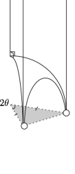
Figure 2: Bilaterally symmetric 3/4-ideal tetrahedron ${\mathcal{L}}(\theta)$ in the half-space model. The shaded isosceles triangle is the shadow cast by the tetrahedron onto the plane at infinity. The circles represent vertices at infinity.

Leibon’s construction is based on the idea of extending all the edges of the tetrahedron to infinity and dissecting the resulting polyhedron into 6 ideal tetrahedra and an ideal octahedron. The construction is identical for hyperideal tetrahedra, as shown in §2, and in this case the convex hull of the 12 ideal vertices is combinatorially equivalent to a truncated tetrahedron. Such a polyhedron can be triangulated by tetrahedra that do not intersect each other, and for this reason it is much easier to see the scissors congruence proof in the hyperideal case. It turns out that there is a “dual” dissection which results in an octahedron whose dihedral angles are supplementary to the angles of the original octahedron. Moreover, it will be shown in §3 that $2T$ can be constructed just from the original octahedron and its dual. In order to get to a decomposition of $T$, we use Dupont’s result in [1] that the group of hyperbolic polyhedra is uniquely 2-divisible. This allows us to literally halve Leibon’s construction by slicing through each of the ${\mathcal{L}}(\theta_{j})$ along its plane of symmetry. This gives the decomposition $T=\coprod_{j=1}^{16}{\mathcal{L}}_{h}(\theta_{j})$, where ${\mathcal{L}}_{h}(\theta_{j})$ is one of the bilaterally symmetric halves of ${\mathcal{L}}(\theta)$. In §4 we show how four of the ${\mathcal{L}}_{h}(\theta_{j})$ and be permuted so that the result is $R_{b}(T)$, the image of $T$ under one of the Regge symmetries.

In an effort to make this paper self-contained, we have summarized the results we will need from [2] in §2 and §3. The exposition of these results in [2] is more general, while the presentation here is geared specifically for what we will need to demonstrate the scissors congruence proof in §4.

I would like to thank Greg Leibon and Peter Doyle for generously sharing their ideas with me. Most of all, thanks to Justin Roberts for introducing us all to this subject.

2 Warm-up for the development Leibon’s set of formulas for the volume of a hyperbolic tetrahedron

In this section we develop the basic idea that is central to Leibon’s geometrization of Murakami and Yano’s formula. Let $T_{3}(A,B,C)$ denote a 3/4-ideal tetrahedron with dihedral angles $A$, $B$, and $C$ at its finite vertex. We now extend the three edges meeting at the non-ideal vertex to infinity obtaining the polyhedron $D$ shown in Figure 3. For simplicity, all the hyperbolic polyhedra from now on will be shown in the Klein model, unless specified otherwise.

Figure 3: Polyhedron $D$

Notice that $D$ is symmetric about the point $p$, so that its volume is twice that of $T_{3}(A,B,C)$. It will be convenient to view $D$ as a simplicial complex which can be triangulated by oriented simplices as follows.

$$D=\{a,b,c,c^{\prime}\}+\{a,a^{\prime},b^{\prime},c^{\prime}\}+\{a,b^{\prime},b,c^{\prime}\},$$ (4)

where $\{x_{1},x_{2},x_{2},x_{4}\}$ denotes the oriented hyperbolic tetrahedron with vertices $x_{1}$, $x_{2}$, $x_{3}$, and $x_{4}$.

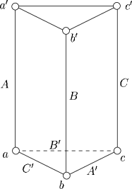
Figure 4: An ideal hyperbolic prism

Now consider the ideal hyperbolic prism, $P$, shown in Figure 4. Viewed as a simplicial complex, $P$ can be triangulated as

$$P=\{a,b,c,c^{\prime}\}+\{a,a^{\prime},b^{\prime},c^{\prime}\}+\{a,b^{\prime},b,c^{\prime}\}.$$ (5)

Equations (4) and (5) indicate that $P$ and $D$ are the same object from the point of view of homology. Clearly, $P$ and $D$ are embedded in space differently. In particular, $P$ is convex while $D$ is not. This is accounted for by the term $\{a,b^{\prime},b,c^{\prime}\}$ in equations (4) and (5). In the case of $D$, $\{a,b^{\prime},b,c^{\prime}\}$ represents a simplex with negative volume, while in the case of $P$, it represents a simplex with positive volume.

Just as $D$ and $P$ are the same object when viewed as simplicial complexes, they are also the same type of object from the point of view of hyperbolic geometry. Both $D$ and $P$ are completely determined by the dihedral angles $A$, $B$, and $C$. In the case of $D$, $A+B+C>\pi$, while in the case of $P$, $A+B+C<\pi$. $P$ can be obtained by a continuous deformation of $D$ which involves moving the point $p$ outside the sphere at infinity (this is easiest seen in the Klein or the hyperboloid model). In this process the angles $A$, $B$, and $C$ decrease. Since the volume of $D$ and $P$ depends only on these three angles, by analytic continuation $D$ and $P$ have the same volume formula. It is easier to see the triangulation of $P$ since the three tetrahedra involved do not intersect each other.

Using the fact that the opposite dihedral angles of an ideal hyperbolic tetrahedron are equal, we find that the tetrahedra in Figure 5 are

$$\{a,b,c,c^{\prime}\} = T(A^{\prime},B^{\prime},C)$$

$$\{a,a^{\prime},b^{\prime},c^{\prime}\} = T(A,B^{\prime},C^{\prime})$$ (6)

$$\{a,b,b^{\prime},c^{\prime}\} = T(C^{\prime}-C,B,\pi-B^{\prime}),$$

where $T(A,B,C)$ denotes an ideal hyperbolic tetrahedron with dihedral angles $A$, $B$, and $C$.

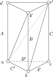
Figure 5: A triangulation of an ideal hyperbolic prism

Applying the condition that the sum of the dihedral angles at an ideal vertex is $\pi$, we obtain

$$A^{\prime}=\frac{\pi+A-B-C}{2}$$

$$B^{\prime}=\frac{\pi+B-A-C}{2}$$ (7)

$$C^{\prime}=\frac{\pi+C-A-B}{2}.$$

By (5), (2) and the famous formula from [3],

$$V(T(\alpha,\beta,\gamma))=\mbox{\cyr L}(\alpha)+\mbox{\cyr L}(\beta)+\mbox{\cyr L}(\gamma),$$ (8)

where $\mbox{\cyr L}(\theta):=-\int_{0}^{\theta}\log 2|\sin u|du$ is the Lobachevsky function, we have

$$2V(\{a,b,c,a^{\prime},b^{\prime},c^{\prime}\})=\mbox{\cyr L}(A)+\mbox{\cyr L}(A^{\prime})+\mbox{\cyr L}(B)+\mbox{\cyr L}(B^{\prime})+\mbox{\cyr L}(C)+\mbox{\cyr L}(C^{\prime})-\\ \mbox{\cyr L}(\frac{\pi+A+B+C}{2}),$$ (9)

where $\{a,b,c,a^{\prime},b^{\prime},c^{\prime}\}$ is either the non-convex prism of Figure 3 or the convex prism of Figure 4.

3 Leibon’s formulas for the volume of a hyperbolic tetrahedron

3.1 The basic setup

We now extend the ideas developed in §2 to a hyperbolic tetrahedron $T$ with finite vertices. We start by extending all the edges of $T$ to infinity. The resulting polyhedron, $C$, is shown in Figure 6, where $T=\{p_{1},p_{2},p_{3},p_{4}\}$. Clearly,

$$V(T)=V(C)-\\ [V(\{c_{1}^{\prime},a_{1},b_{1}^{\prime},p_{1}\})+V(\{a_{1}^{\prime},b_{2}^{\prime},c_{1},p_{2}\})+V(\{a_{2}^{\prime},b_{1},c_{2}^{\prime},p_{3}\})+V(\{a_{2},b_{2},c_{2},p_{4}\})]$$ (10)

Since the 4 tetrahedra on the right hand side of (10) are all 3/4-ideal, their volume is given by (9). Therefore, the main task at hand is to calculate the volume of $C$. In order to triangulate $C$, we first note that it is the same object as $U$ (see Figure 7) from the point of view of homology, following the method of §2. That is, $U$ can be obtained from $C$ by pulling the points $p_{1}$, $p_{2}$, $p_{3}$, and $p_{4}$ outside the sphere at infinity. Under this deformation the non-convex prisms $\{c_{1}^{\prime},a_{1},b_{1}^{\prime},c_{2}^{\prime},a_{2},b_{2}^{\prime}\}$, $\{a_{1}^{\prime},b_{2}^{\prime},c_{1},a_{2}^{\prime},b_{1}^{\prime},c_{2}\}$, $\{a_{2}^{\prime},b_{1},c_{2}^{\prime},a_{1}^{\prime},b_{2},c_{1}^{\prime}\}$, and $\{a_{2},b_{2},c_{2},a_{1},b_{1},c_{1}\}$ become convex, but their volume formula stays the same by analytic continuation. Thus

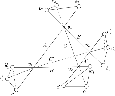
Figure 6: Polyhedron $C$

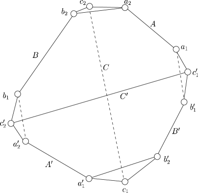
Figure 7: Polyhedron $U$

$$V(T)=V(U)-V(\{c_{1}^{\prime},a_{1},b_{1}^{\prime},c_{2}^{\prime},a_{2},b_{2}^{\prime}\})/2-V(\{a_{1}^{\prime},b_{2}^{\prime},c_{1},a_{2}^{\prime},b_{1}^{\prime},c_{2}\})/2\\ -V(\{a_{2}^{\prime},b_{1},c_{2}^{\prime},a_{1}^{\prime},b_{2},c_{1}^{\prime}\})/2-V(\{a_{2},b_{2},c_{2},a_{1},b_{1},c_{1}\})/2.$$ (11)

Since a triangulation of $C$ by oriented simplices is also a triangulation of $U$, we may as well work with $U$. This is easier than working with $C$ because the tetrahedra in the triangulation of $U$ do not intersect each other. Everything that follows applies equally well to finite as well as hyperideal tetrahedra.

In order to compute the volume of $U$ we triangulate it using only ideal tetrahedra and the compute the volume of each of these tetrahedra using (8). It turns out that no matter which way $U$ is triangulated, some of the tetrahedra comprising it will have dihedral angles that are affine functions of the dihedral angles of $T$, while others will not. Leibon has looked at a particular family of $2^{6}$ triangulations of $U$, each of which divides up $U$ into six tetrahedra and one octahedron. The number $2^{6}$ comes from the fact that the vertices of the octahedron can be chosen by selecting exactly one of the vertices in each pair $\{a_{1},a_{2}\}$, $\{b_{1},b_{2}\}$, $\{c_{1},c_{2}\}$, $\{a_{1}^{\prime},a_{2}^{\prime}\}$, $\{b_{1}^{\prime},b_{2}^{\prime}\}$, $\{c_{1}^{\prime},c_{2}^{\prime}\}$. If one chooses both or neither of the vertices in any pair, then it is impossible to form a non-degenerate octahedron with the remaining vertices.

We will illustrate the computation of the volume of $U$ using the partial triangulation shown in Figure 8. The prism and three tetrahedra resulting from this decomposition are shown in Figure 9, while the octahedron $O$ is shown in Figure 10. The prism in Figure 9 can be decomposed into three ideal tetrahedra, as demonstrated in §2. In Figure 9, the dihedral angles other than those belonging to the original tetrahedron $T$ were computed with the help of (2). For example, the dihedral angle at the edge $\{a_{1},c_{1}^{\prime}\}$ was computed by considering the prism $\{c_{1}^{\prime},a_{1},b_{1}^{\prime},c_{2}^{\prime},a_{2},b_{2}^{\prime}\}$. Since the dihedral angles at each pair of opposite edges of an ideal tetrahedron are equal, the labels in Figure 9 are enough to completely determine each tetrahedron. The dihedral angles of the octahedron $O$ then follow immediately.

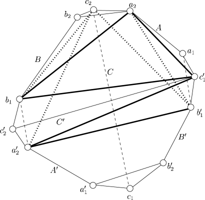
Figure 8: Decomposition of polyhedron $U$. The edges of $U$ are shown with thin and dashed lines, while the cuts of the decomposition are shown with thicker and dotted lines.

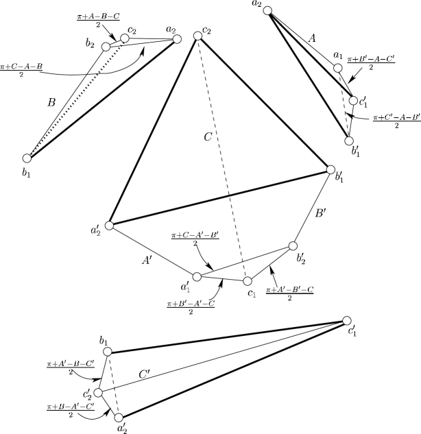
Figure 9: Decomposition of polyhedron $U$, Part I: the tetrahedra

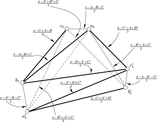
Figure 10: Decomposition of polyhedron $U$, Part II: the octahedron $O$

3.2 Triangulating the octahedron

The octahedron in Figure 10 can be triangulated by drawing an edge from one of its vertices to a non-adjacent vertex. There are three distinct ways to do this. No matter which way is chosen, the dihedral angles of the resulting four tetrahedra can be determined by a family of 7 linear equations and one quadratic equation.

The following terminology will be used to describe the triangulation of an octahedron.

Definition 3.1.

The firepole of an octahedron is a segment joining one of its vertices to a non-adjacent vertex.

In Figure 10 the firepole is the dashed line connecting vertices $a_{2}$ and $a_{2}^{\prime}$. At this point it is easier to view $O$ in the half-space model, with the vertex $a_{2}$ at the point at infinity. This is depicted in Figure 11. The segments $\{a_{2},c_{1}^{\prime}\}$, $\{a_{2},b_{1}^{\prime}\}$, $\{a_{2},c_{2}\}$, $\{a_{2},b_{1}\}$ become lines perpendicular to the plane at infinity in the half-space model, and their projection is seen in Figure 11 as vertices $v_{a}$, $v_{b}$, $v_{c}$, and $v_{d}$.

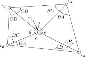
Figure 11: Octahedron $O$ in the half-space model

The angles of the quadrilateral at each of these vertices are $a$, $b$, $c$, and $d$, and they are equal to the angles dihedral angles of $O$ at edges $\{v_{0},v_{a}\}$, $\{v_{0},v_{b}\}$, $\{v_{0},v_{c}\}$, and $\{v_{0},v_{d}\}$, since the half-space model is conformal. As seen in Figure 10, these angles are

$$\begin{split}a=\frac{\pi-C^{\prime}+A+B^{\prime}}{2};\;\;b=\frac{\pi-B^{\prime}+A+C^{\prime}}{2}\\ c=\frac{\pi-A-B-C}{2};\;\;d=\frac{\pi-A+B+C}{2}.\end{split}$$ (12)

The edges with dihedral angles $e$, $f$, $g$, $h$ are opposite to edges $\{v_{a},v_{b}\}$, $\{v_{b},v_{c}\}$, $\{v_{c},v_{d}\}$, $\{v_{d},v_{a}\}$, respectively, and the angles at those edges have already been computed (see Figure 10). Using the fact that opposite edges of an ideal tetrahedron have equal dihedral angles, we have

$$\begin{split}e=\frac{\pi-A-B^{\prime}-C^{\prime}}{2};\;\;f=\frac{\pi-A^{\prime}+B^{\prime}+C}{2}\\ g=\frac{\pi-C+A+B}{2};\;\;h=\frac{\pi-B+A^{\prime}+C^{\prime}}{2}.\end{split}$$ (13)

The unknown angles have been denoted as $AB$, $BA$, $BC$, $CB$, $CD$, $DC$, $DA$, and $AD$. These angles are subject to the following linear constraints:

$$\begin{split}AB+AD=a;\;\;&AB+BA+e=\pi\\ BC+BA=b;\;\;&BC+CB+f=\pi\\ CD+CB=c;\;\;&CD+DC+g=\pi\\ DA+DC=d;\;\;&DA+AD+h=\pi.\end{split}$$ (14)

The matrix expressing conditions (14) has a one-dimensional null space, so one more condition is needed to determine the 8 unknown angles. Geometrically, this last condition insures that the four ideal tetrahedra fit together. In other words, one can always fit together four tetrahedra that satisfy (14) as shown in Figure 12, since the faces of all ideal tetrahedra are ideal triangles, and, therefore, isometric to one another.

Figure 12: Four tetrahedra that satisfy equations (14)

In order avoid the situation in Figure 12, we need to insure that once we fit the four tetrahedra together, the Euclidean length of the segment $\{v_{0},v_{a}\}$ does not change as we go around the quadrilateral $\{v_{a},v_{b},v_{c},v_{d}\}$. In particular, if we assume that the length of the segment $\{v_{0},v_{a}\}$ is equal to 1, then express it in terms of the other lengths of the quadrilateral and equate the two quantities, we will get a non-trivial condition that, together with equations (14), will determine the unknown angles in Figure 11.

The equation we need is

$$\frac{\sin(AB)}{\sin(BA)}\frac{\sin(BC)}{\sin(CB)}\frac{\sin(CD)}{\sin(DC)}\frac{\sin(DA)}{\sin(AD)}=1,$$ (15)

and Figure 13 suggests how it is obtained.

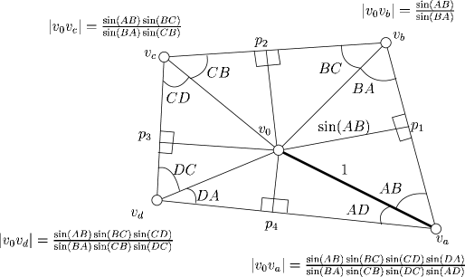
Figure 13: Non-linear condition for insuring that four tetrahedra fit together to make an octahedron

Since scaling is an isometry in hyperbolic space, we may assume without loss of generality that the Euclidean length of the segment $\{v_{0},v_{a}\}$ is 1. Then by going counter-clockwise around Figure 13 and using basic trigonometry we obtain

$$|v_{0}p_{1}| = \sin(AB)$$

$$|v_{0}v_{b}| = |v_{0}p_{1}|/\sin(BA)$$

$$= \sin(AB)/\sin(BA),$$

and so on, until finally we arrive at the two equivalent expressions for $|v_{0}v_{a}|$ in (15).

It is easier to solve the system of equations (14) and (15) if we first come up with a solution in the one-dimensional space that satisfies (14) and then use (15) to find the remaining unknown. Let $(\overline{AB},\overline{BA},\overline{BC},\overline{CB},\overline{CD},\overline{DC},\overline{DA},\overline{AD})$ be a solution to the system of equations (14). Then there must be a $Z$ such that

$$\begin{split}\overline{AB}+Z=AB;\;\;&\overline{BA}-Z=BA\\ \overline{BC}+Z=BC;\;\;&\overline{CB}-Z=CB\\ \overline{CD}+Z=CD;\;\;&\overline{DC}-Z=DC\\ \overline{DA}+Z=DA;\;\;&\overline{AD}-Z=AD.\end{split}$$ (16)

No matter what the value of $Z$ is, the quantities on the right hand side of equations (16) still satisfy equations (14), since the sums in those equations are unchanged when $Z$ is added to one summand and subtracted from the other one. After substituting (16) into (15), letting $z=\exp(iZ)$ and

$$\begin{split}\alpha_{1}=\exp(i\overline{AB});\;\;\beta_{1}=\exp(i\overline{BA})\\ \alpha_{2}=\exp(i\overline{BC});\;\;\beta_{2}=\exp(i\overline{CB})\\ \alpha_{3}=\exp(i\overline{CD});\;\;\beta_{3}=\exp(i\overline{DC})\\ \alpha_{4}=\exp(i\overline{DA});\;\;\beta_{4}=\exp(i\overline{AD}),\end{split}$$ (17)

we obtain

$$0=\frac{1}{\alpha_{1}\alpha_{2}\alpha_{3}\alpha_{4}}-\beta_{1}\beta_{2}\beta_{3}\beta_{4}+z^{2}(-\frac{\alpha_{1}}{\alpha_{2}\alpha_{3}\alpha_{4}}-\frac{\alpha_{2}}{\alpha_{1}\alpha_{3}\alpha_{4}}-\frac{\alpha_{3}}{\alpha_{1}\alpha_{2}\alpha_{4}}-\frac{\alpha_{4}}{\alpha_{1}\alpha_{2}\alpha_{3}}\\ +\frac{\beta_{1}\beta_{2}\beta_{3}}{\beta_{4}}+\frac{\beta_{1}\beta_{2}\beta_{4}}{\beta_{3}}+\frac{\beta_{1}\beta_{3}\beta_{4}}{\beta_{2}}+\frac{\beta_{2}\beta_{3}\beta_{4}}{\beta_{1}})\\ +z^{4}(\frac{\alpha_{1}\alpha_{2}}{\alpha_{3}\alpha_{4}}+\frac{\alpha_{1}\alpha_{3}}{\alpha_{2}\alpha_{4}}+\frac{\alpha_{2}\alpha_{3}}{\alpha_{1}\alpha_{4}}+\frac{\alpha_{1}\alpha_{4}}{\alpha_{2}\alpha_{3}}+\frac{\alpha_{2}\alpha_{4}}{\alpha_{1}\alpha_{3}}+\frac{\alpha_{3}\alpha_{4}}{\alpha_{1}\alpha_{2}}\\ -\frac{\beta_{1}\beta_{2}}{\beta_{3}\beta_{4}}-\frac{\beta_{1}\beta_{3}}{\beta_{2}\beta_{4}}-\frac{\beta_{2}\beta_{3}}{\beta_{1}\beta_{4}}-\frac{\beta_{1}\beta_{4}}{\beta_{2}\beta_{3}}-\frac{\beta_{2}\beta_{4}}{\beta_{1}\beta_{3}}-\frac{\beta_{3}\beta_{4}}{\beta_{1}\beta_{2}})\\ +z^{6}(\frac{\beta_{1}}{\beta_{2}\beta_{3}\beta_{4}}+\frac{\beta_{2}}{\beta_{1}\beta_{3}\beta_{4}}+\frac{\beta_{3}}{\beta_{1}\beta_{2}\beta_{4}}+\frac{\beta_{4}}{\beta_{1}\beta_{2}\beta_{3}}\\ -\frac{\alpha_{1}\alpha_{2}\alpha_{3}}{\alpha_{4}}-\frac{\alpha_{1}\alpha_{2}\alpha_{4}}{\alpha_{3}}-\frac{\alpha_{1}\alpha_{3}\alpha_{4}}{\alpha_{2}}-\frac{\alpha_{2}\alpha_{3}\alpha_{4}}{\alpha_{1}})+z^{8}(\alpha_{1}\alpha_{2}\alpha_{3}\alpha_{4}-\frac{1}{\beta_{1}\beta_{2}\beta_{3}\beta_{4}}).$$ (18)

By equations (14) and (16),

$$(\overline{AB}+\overline{BC}+\overline{CD}+\overline{DA})+(\overline{BA}+\overline{CB}+\overline{DC}+\overline{AD})=2\pi,$$

so that

$$\alpha_{1}\alpha_{2}\alpha_{3}\alpha_{4}=\frac{1}{\beta_{1}\beta_{2}\beta_{3}\beta_{4}}.$$

This reduces (18) to a quadratic equaton in $z^{2}$.

Let $z_{+}$ ($z_{-}$) denote the solution of (18) corresponding to adding (subtracting) the square root of the discriminant. Then $z_{-}$ gives the correct values of the angles of the octahedron $O$ in Figure 10, while $z_{+}$ is of great significance as well and will be discussed in §3.4.

3.3 Computation of the volume formula using the root $z_{-}$ of equation (18)

At this point we can write down the volume of the octahedron $O$ (see Figure 11) using formula (8) for the volume of an ideal hyperbolic tetrahedron:

$$V(O) = V(\{v_{a},v_{b},v_{0},\infty\})+V(\{v_{b},v_{c},v_{0},\infty\})+$$ (19)

$$V(\{v_{c},v_{d},v_{0},\infty\})+V(\{v_{d},v_{a},v_{0},\infty\})$$

$$= \mbox{\cyr L}(AB)+\mbox{\cyr L}(BA)+\mbox{\cyr L}(e)+\mbox{\cyr L}(BC)+\mbox{\cyr L}(CB)+\mbox{\cyr L}(f)$$

$$\mbox{\cyr L}(CD)+\mbox{\cyr L}(DC)+\mbox{\cyr L}(g)+\mbox{\cyr L}(DA)+\mbox{\cyr L}(AD)+\mbox{\cyr L}(h).$$

Substituting (16) and (13) into (19) and setting $Z=\arg z_{-}$, we have

$$V(O)=\mbox{\cyr L}(\overline{AB}+\arg z_{-})+\mbox{\cyr L}(\overline{BA}-\arg z_{-})+\mbox{\cyr L}(\overline{BC}+\arg z_{-})\\ +\mbox{\cyr L}(\overline{CB}-\arg z_{-})+\mbox{\cyr L}(\overline{CD}+\arg z_{-})+\mbox{\cyr L}(\overline{DC}-\arg z_{-})\\ +\mbox{\cyr L}(\overline{DA}+\arg z_{-})+\mbox{\cyr L}(\overline{AD}-\arg z_{-})+\mbox{\cyr L}(\frac{\pi-A-B^{\prime}-C^{\prime}}{2})\\ +\mbox{\cyr L}(\frac{\pi-A^{\prime}+B^{\prime}+C}{2})+\mbox{\cyr L}(\frac{\pi-C+A+B}{2})+\mbox{\cyr L}(\frac{\pi-B+A^{\prime}+C^{\prime}}{2}),$$ (20)

where $\overline{AB}$, etc. are chosen as

$$\begin{split}&\overline{AB}=\frac{A+A^{\prime}+2B^{\prime}}{4};\;\;\overline{BA}=\frac{2\pi+A-A^{\prime}+2C^{\prime}}{4}\\ &\overline{BC}=\frac{A+A^{\prime}-2B^{\prime}}{4};\;\;\overline{CB}=\frac{2\pi-A+A^{\prime}-2C}{4}\\ &\overline{CD}=\frac{-A-A^{\prime}-2B}{4};\;\;\overline{DC}=\frac{2\pi-A+A^{\prime}+2C}{4}\\ &\overline{DA}=\frac{-A-A^{\prime}+2B}{4};\;\;\overline{AD}=\frac{2\pi+A-A^{\prime}-2C^{\prime}}{4}.\end{split}$$ (21)

Using (20) along with the volumes of the three tetrahedra and prism in Figure 9 and the fact that L is odd and $\pi$-periodic gives

$$V(U) = \mbox{\cyr L}(\overline{AB}+\arg z_{-})+\mbox{\cyr L}(\overline{BA}-\arg z_{-})+$$ (22)

$$\mbox{\cyr L}(\overline{BC}+\arg z_{-})+\mbox{\cyr L}(\overline{CB}-\arg z_{-})+$$

$$\mbox{\cyr L}(\overline{CD}+\arg z_{-})+\mbox{\cyr L}(\overline{DC}-\arg z_{-})+$$

$$\mbox{\cyr L}(\overline{DA}+\arg z_{-})+\mbox{\cyr L}(\overline{AD}-\arg z_{-})+$$

$$+\mbox{\cyr L}(A)+\mbox{\cyr L}(A^{\prime})+\mbox{\cyr L}(B)+\mbox{\cyr L}(B^{\prime})+\mbox{\cyr L}(C)+\mbox{\cyr L}(C^{\prime})$$

$$+\mbox{\cyr L}(\frac{\pi-A-B^{\prime}-C^{\prime}}{2})+\mbox{\cyr L}(\frac{\pi+A^{\prime}-B-C^{\prime}}{2})$$

$$+\mbox{\cyr L}(\frac{\pi+B^{\prime}-A-C^{\prime}}{2})+\mbox{\cyr L}(\frac{\pi+C^{\prime}-A-B^{\prime}}{2})$$

$$+\mbox{\cyr L}(\frac{\pi+A-B-C}{2})+\mbox{\cyr L}(\frac{\pi+C-A^{\prime}-B^{\prime}}{2})$$

$$+\mbox{\cyr L}(\frac{\pi+B^{\prime}-A^{\prime}-C}{2})-\mbox{\cyr L}(\frac{\pi+A^{\prime}+B^{\prime}+C}{2}).$$

Finally, plugging (22) into (11) and using formula (9) for the volume of an ideal prism gives

$$V(T)=\mbox{\cyr L}(\overline{AB}+\arg z_{-})+\mbox{\cyr L}(\overline{BA}-\arg z_{-})+\mbox{\cyr L}(\overline{BC}+\arg z_{-})\\ +\mbox{\cyr L}(\overline{CB}-\arg z_{-})+\mbox{\cyr L}(\overline{CD}+\arg z_{-})+\mbox{\cyr L}(\overline{DC}-\arg z_{-})\\ +\mbox{\cyr L}(\overline{DA}+\arg z_{-})+\mbox{\cyr L}(\overline{AD}-\arg z_{-})+\frac{1}{2}[\mbox{\cyr L}(\frac{\pi+A-B-C}{2}\\ -\mbox{\cyr L}(\frac{\pi+B-A-C}{2})-\mbox{\cyr L}(\frac{\pi+C-A-B}{2})+\mbox{\cyr L}(\frac{\pi+B^{\prime}-A^{\prime}-C}{2})\\ +\mbox{\cyr L}(\frac{\pi+A+B+C}{2})+\mbox{\cyr L}(\frac{\pi+C-A^{\prime}-B^{\prime}}{2})+\mbox{\cyr L}(\frac{\pi-A^{\prime}+B^{\prime}+C}{2})\\ -\mbox{\cyr L}(\frac{\pi+A^{\prime}+B^{\prime}+C}{2})+\mbox{\cyr L}(\frac{\pi+A^{\prime}-B-C^{\prime}}{2}-\mbox{\cyr L}(\frac{\pi+A+B^{\prime}+C^{\prime}}{2})\\ -\mbox{\cyr L}(\frac{\pi+A-B^{\prime}-C^{\prime}}{2})+\mbox{\cyr L}(\frac{\pi+B^{\prime}-A-C^{\prime}}{2})-\mbox{\cyr L}(\frac{\pi-A^{\prime}-B+C^{\prime}}{2})\\ +\mbox{\cyr L}(\frac{\pi+A^{\prime}-B+C^{\prime}}{2})+\mbox{\cyr L}(\frac{\pi+A^{\prime}+B+C^{\prime}}{2})+\mbox{\cyr L}(\frac{\pi-A-B^{\prime}+C^{\prime}}{2})],$$ (23)

where the quantities with bars are given by (21), and $z_{-}$ is the solution of the quadratic equation (18) with the negative square root.

3.4 Computation of the volume formula using the root $z_{+}$ of equation (18)

When $z_{-}$ is replaced by $z_{+}$ in equation (23) one gets $-V(T)$ instead of $V(T)$. This surprising result has a very concrete geometrical explanation. The main idea is that the octahedron $O$ has a dual octahedron $O^{\prime}$ associated with it, and that $V(T)$ can be expressed in terms of either $O$ or $O^{\prime}$. It will be shown below that the solution $z_{+}$ of (18) solves the angles of a triangulation of the octahedron $O^{\prime}$.

Recall formula (11) in §3.1, which indicates that we can construct a tetrahedron $T$ by subtracting 4 half-prisms from the tetrahedron $U$ (see Figure 7). Let $H_{P}$ denote one of the symmetric halves of a triangular prism $P$. So, for example, if $P$ is the triangular prism $\{a,b,c,a^{\prime},b^{\prime},c^{\prime}\}$ in Figure 14, $H_{P}=\{a,b,c,m_{1},m_{2},m_{3}\}$.

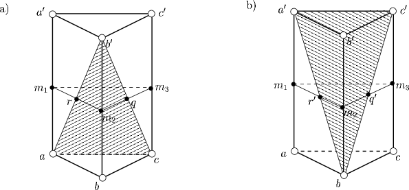
Figure 14: Subdivisions of a triangular prism

We will now show how to recast equation (11) as a decomposition. First, let us recall the construction of the octahedron $O$. As described earlier, $O$ (see Figure 10) was constructed by selecting one vertex from each edge of $U$ (see Figure 8). It follows that each of the four hexagonal faces of $U$ coincides with a face of $O$. There is a one-to-one correspondence between the other four faces of $O$ and the four prisms

$$P_{1} = \{c_{1}^{\prime},a_{1},b_{1}^{\prime},c_{2}^{\prime},a_{2},b_{2}^{\prime}\}$$

$$P_{2} = \{a_{1}^{\prime},b_{2}^{\prime},c_{1},a_{2}^{\prime},b_{1}^{\prime},c_{2}\}$$

$$P_{3} = \{a_{2}^{\prime},b_{1},c_{2}^{\prime},a_{1}^{\prime},b_{2},c_{1}^{\prime}\}$$

$$P_{4} = \{a_{2},b_{2},c_{2},a_{1},b_{1},c_{1}\}.$$

Formula (11) can then be expressed as follows:

$$T = U-H_{P_{1}}-H_{P_{2}}-H_{P_{3}}-H_{P_{4}}$$ (24)

$$= O+$$

$$\{c_{1}^{\prime},a_{1},b_{1}^{\prime},a_{2}\}+\{a_{1}^{\prime},b_{2}^{\prime},c_{1},a_{2}^{\prime},b_{1}^{\prime},c_{2}\}+\{a_{2}^{\prime},b_{1},c_{2}^{\prime},c_{1}^{\prime}\}+\{a_{2},b_{2},c_{2},b_{1}\}$$

$$-H_{P_{1}}-H_{P_{2}}-H_{P_{3}}-H_{P_{4}}.$$

We now introduce $O^{\prime}$, the octahedron dual to $O$. With Figure 8 in mind, one can visualize sliding the vertices of $O$, $\{a_{2},c_{2},b_{1},a_{2}^{\prime},b_{1}^{\prime},c_{1}^{\prime}\}$, along the respective edges labeled as $A$, $B$, $C$, $A^{\prime}$, $B^{\prime}$, $C^{\prime}$ until they hit the vertices at the end of these edges. We define the resulting octahedron as $O^{\prime}$. In other words $O^{\prime}$ is the convex hull of the vertices $\{a_{1},c_{1},b_{2},a_{1}^{\prime},b_{2}^{\prime},c_{2}^{\prime}\}$. We can now express $U$ as

$$U=O^{\prime}+\{c_{1}^{\prime},b_{1}^{\prime},b_{2}^{\prime},c_{2}^{\prime},a_{1}\}+\{\emptyset\}+\{a_{1}^{\prime},b_{2},b_{1},a_{2}^{\prime},c_{2}^{\prime}\}+\{a_{1},a_{2},c_{2},c_{1},b_{2}\},$$ (25)

so that

$$T=O^{\prime}+\{c_{1}^{\prime},b_{1}^{\prime},b_{2}^{\prime},c_{2}^{\prime},a_{1}\}+\{\emptyset\}+\{a_{1}^{\prime},b_{2},b_{1},a_{2}^{\prime},c_{2}^{\prime}\}+\{a_{1},a_{2},c_{2},c_{1},b_{2}\}\\ -H_{P_{1}}-H_{P_{2}}-H_{P_{3}}-H_{P_{4}}.$$ (26)

We claim that

$$2T=O+O^{\prime}.$$ (27)

To verify this claim, let us look back at Figure 8 and how the last 8 terms of (24) are situated with respect to one another inside the polyhedron $U$. It is clear that there are some partial cancellations between pairs of certain terms. For example, the polyhedra $\{c_{1}^{\prime},a_{1},b_{1}^{\prime},a_{2}\}$ and $H_{P_{1}}$ overlap. To see exactly what happens, it is helpful to compare $P_{1}=\{c_{1}^{\prime},a_{1},b_{1}^{\prime},c_{2}^{\prime},a_{2},b_{2}^{\prime}\}$ to the prism $\{a,b,c,a^{\prime},b^{\prime},c^{\prime}\}$ in Figure 14(a). $\{c_{1}^{\prime},a_{1},b_{1}^{\prime},a_{2}\}$ corresponds to $\{a,b,c,b^{\prime}\}$, and $H_{P_{1}}$ corresponds to $\{a,b,c,m_{1},m_{2},m_{3}\}$. It follows immediately from Figure 14(a) that

$$\{a,b,c,b^{\prime}\}=\{a,b,c,r,m_{2},q\}+\{r,m_{2},q,b^{\prime}\},$$ (28)

and

$$\{a,b,c,m_{1},m_{2},m_{3}\}=\{a,b,c,r,m_{2},q\}+\{a,c,m_{3},m_{1},q,r\}.$$ (29)

Subtracting (29) from (28) gives

$$\{a,b,c,b^{\prime}\}-\{a,b,c,m_{1},m_{2},m_{3}\}=\{r,m_{2},q,b^{\prime}\}-\{a,c,m_{3},m_{1},q,r\}.$$ (30)

Now, the decomposition of $T$ in terms of $O^{\prime}$ in (26) is obtained from the decomposition in (24) by sliding all the vertices of $O$ to the opposite ends of the edges. So, for example, the tetrahedron $\{c_{1}^{\prime},a_{1},b_{1}^{\prime},a_{2}\}$ in (24) gets replaced by the pyramid $\{c_{1}^{\prime},b_{1}^{\prime},b_{2}^{\prime},c_{2}^{\prime},a_{1}\}$ in (26). One can see this in Figure 14, where the tetrahedron $\{a,b,c,b^{\prime}\}$ corresponding to $\{c_{1}^{\prime},a_{1},b_{1}^{\prime},a_{2}\}$ is replaced by the pyramid $\{a,c,c^{\prime},a^{\prime},b\}$ corresponding to $\{c_{1}^{\prime},b_{1}^{\prime},b_{2}^{\prime},c_{2}^{\prime},a_{1}\}$ after the vertices $a$, $c$, and $b^{\prime}$ are slid to $a^{\prime}$, $c^{\prime}$, and $b$.

As before, we wish to write the expression $\{c_{1}^{\prime},b_{1}^{\prime},b_{2}^{\prime},c_{2}^{\prime},a_{1}\}-H_{P_{1}}$ in (26) as a sum of disjoint simplices. Figure 14(b) gives

$$\{a,c,c^{\prime},a^{\prime},b\}=\{a,b,c,m_{1},r^{\prime},m_{2},q^{\prime},m_{3}\}+\{a^{\prime},c^{\prime},m_{1},m_{3},q^{\prime},r^{\prime}\}$$

and

$$\{a,b,c,m_{1},m_{2},m_{3}\}=\{a,b,c,m_{1},r^{\prime},m_{2},q^{\prime},m_{3}\}+\{m_{2},r^{\prime},q^{\prime},b\}.$$

Thus

$$\{a,c,c^{\prime},a^{\prime},b\}-\{a,b,c,m_{1},m_{2},m_{3}\}=\{a^{\prime},c^{\prime},m_{1},m_{3},q^{\prime},r^{\prime}\}-\{m_{2},r^{\prime},q^{\prime},b\}.$$ (31)

Comparing the right hand sides of (30) and (31) we find that they are negatives of one another. This is because $\{r,m_{2},q,b^{\prime}\}$ and $\{a,c,m_{3},m_{1},q,r\}$ are isometric to $\{m_{2},r^{\prime},q^{\prime},b\}$ and $\{a^{\prime},c^{\prime},m_{1},m_{3},q^{\prime},r^{\prime}\}$, respectively, by the symmetry of the prism. It follows that the same relationship holds between the corresponding terms in (24) and (26):

$$\{c_{1}^{\prime},a_{1},b_{1}^{\prime},a_{2}\}-H_{P_{1}}=-[\{c_{1}^{\prime},b_{1}^{\prime},b_{2}^{\prime},c_{2}^{\prime},a_{1}\}-H_{P_{1}}].$$

It is easy to verify that the analagous relationship holds between the remaining pairs of terms in (24) and (26). Therefore,

$$-[\{c_{1}^{\prime},a_{1},b_{1}^{\prime},a_{2}\}+\{a_{1}^{\prime},b_{2}^{\prime},c_{1},a_{2}^{\prime},b_{1}^{\prime},c_{2}\}+\{a_{2}^{\prime},b_{1},c_{2}^{\prime},c_{1}^{\prime}\}+\{a_{2},b_{2},c_{2},b_{1}\}\\ -H_{P_{1}}-H_{P_{2}}-H_{P_{3}}-H_{P_{4}}]=\\ \{c_{1}^{\prime},b_{1}^{\prime},b_{2}^{\prime},c_{2}^{\prime},a_{1}\}+\{a_{1}^{\prime},b_{2},b_{1},a_{2}^{\prime},c_{2}^{\prime}\}+\{a_{1},a_{2},c_{2},c_{1},b_{2}\}-H_{P_{1}}-H_{P_{2}}-H_{P_{3}}-H_{P_{4}}.$$

Equation (27) then follows from adding (24) and (26).

Thus we have demonstrated that twice a hyperbolic tetrahedron is scissors congruent to two octahedra, $O$ and $O^{\prime}$. This fact will be used extensively in the next section to prove that the Regge symmetry is a scissors congruence.

All that remains to be shown is that by replacing $z_{-}$ with $z_{+}$ in (20) one is swapping $V(O)$ for $-V(O^{\prime})$. To see this, let us examine the quantitative relationship between $O$ and $O^{\prime}$. Recall Figure 14, where we saw that $\{a,b,c,b^{\prime}\}$ is isometric to $\{c^{\prime},b^{\prime},a^{\prime},b\}$. As stated earlier, we can visualize the process of getting from Figure 14(a) to Figure 14(b) as sliding the vertices $a$, $b^{\prime}$, $c$ along the edges $\{a,a^{\prime}\}$, $\{b,b^{\prime}\}$, $\{c,c^{\prime}\}$, respectively. If we measure the change in the angle $\theta$ between the oriented planes determined by $\{a,c,b^{\prime}\}$ and $\{a,b,b^{\prime}\}$ during this process, we find that $\theta$ changes to $\pi-\theta$ in Figure 14(b). Extending this process to $O$ and $O^{\prime}$, we see that dihedral angles of $O$ and $O^{\prime}$ are supplementary, as shown in the Klein model drawings in Figure 15.

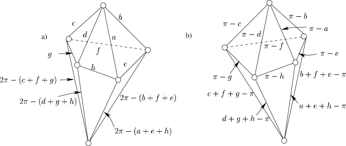
Figure 15: a) The original octahedron $O$ with its dihedral angles labeledb) The dual octahedron $O^{\prime}$

We can now apply the triangulation and computations described in §3.2 and §3.3 to $O^{\prime}$. This will yield a system of linear equations similar to (16) and a non-linear constraint like (15). Choosing

$$(-\overline{AB},-\overline{BC},-\overline{CD},-\overline{DA},\pi-\overline{BA},\pi-\overline{CB},\pi-\overline{DC},\pi-\overline{AD})$$

as a solution to the system of linear equations results in a quadratic equation which turns out to be the same as (18). It follows that the second root of (18) solves for the unknown angles of the triangulation of $O^{\prime}$. It is then easy to verify the following lemma.

Lemma 3.2.

Replacing $z_{-}$ with $z_{+}$ in (20) results in the negative of the volume of $O^{\prime}$.

It follows that the root $z_{+}$ yields $-V(T)$ when substituted for $z_{-}$ in (23). We can use this fact to derive the following expression for the volume of $T$:

$$2V(T)=\mbox{\cyr L}(\overline{AB}+\arg z_{-})+\mbox{\cyr L}(\overline{BA}-\arg z_{-})+\mbox{\cyr L}(\overline{BC}+\arg z_{-})\\ +\mbox{\cyr L}(\overline{CB}-\arg z_{-})+\mbox{\cyr L}(\overline{CD}+\arg z_{-})+\mbox{\cyr L}(\overline{DC}-\arg z_{-})\\ +\mbox{\cyr L}(\overline{DA}+\arg z_{-})+\mbox{\cyr L}(\overline{AD}-\arg z_{-})+\mbox{\cyr L}(-\overline{AB}+\arg z_{+})\\ -\mbox{\cyr L}(\overline{BA}+\arg z_{+})+\mbox{\cyr L}(-\overline{BC}+\arg z_{+})-\mbox{\cyr L}(\overline{CB}+\arg z_{+})\\ +\mbox{\cyr L}(-\overline{CD}+\arg z_{+})-\mbox{\cyr L}(\overline{DC}+\arg z_{+})+\mbox{\cyr L}(-\overline{DA}+\arg z_{+})\\ -\mbox{\cyr L}(\overline{AD}+\arg z_{+}).$$ (32)

4 Generating the Regge symmetries by scissors congruence

Based on formulas (27) and (32) we can now construct a simple proof that $2T$ is scissors congruent to $2R(T)$, where $R$ denotes any compositon of $R_{a}$, $R_{b}$, and $R_{c}$ as defined in (1), (2), and (3).

Recall Figure 11, which shows a triangulation of $O$ in the half-space model. In other words,

$$O=\{v_{a},v_{b},v_{0},\infty\}+\{v_{b},v_{c},v_{0},\infty\}+\{v_{c},v_{d},v_{0},\infty\}+\{v_{d},v_{a},v_{0},\infty\}.$$ (33)

We will now subdivide each of the tetrahedra $\{v_{a},v_{b},v_{0},\infty\}$, $\{v_{b},v_{c},v_{0},\infty\}$,
$\{v_{c},v_{d},v_{0},\infty\}$, and $\{v_{d},v_{a},v_{0},\infty\}$ into three tetrahedra just as Milnor did in his derivation of (8). This is illustrated in Figure 16, where the dotted vertical line is a perpendicular dropped from the vertex at the point of infinity, denoted by $\infty$, to the face opposite to it, $\{a,b,c\}$.

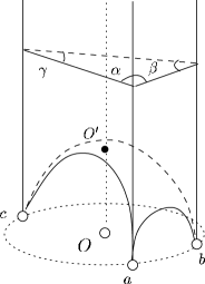
Figure 16: An ideal hyperbolic tetrahedron in the half-space model

This line must meet the plane at infinity at the center of the hemisphere that determines $\{a,b,c\}$. In other words, the projection of this configuration onto the plane at infinity looks like Figure 17, where the end of the perpendicular coincides with the circumcenter of the triangle determined by $a$, $b$, and $c$.

Figure 17: The projection of Figure 16 onto the plane at infinity

Thus we see from Figure 16 that $\{b,c,O^{\prime},\infty\}$, $\{c,a,O^{\prime},\infty\}$, and $\{a,b,O^{\prime},\infty\}$ are ${\mathcal{L}}(\alpha)$, ${\mathcal{L}}(\beta)$, and ${\mathcal{L}}(\gamma)$, respectively.

We now apply this construction to the 4 tetrahedra that triangulate the octahedron in Figures 10 and  11, ending up with 12 tetrahedra each of which has 3 ideal vertices and 1 non-ideal vertex. The projection of this construction onto the plane at infinity is shown in Figure 18. In that figure, the projections of the vertices $p_{e}$, $p_{f}$, $p_{g}$, and $p_{h}$ are the respective circumcenters of the triangles $v_{a}v_{b}v_{0}$, $v_{b}v_{c}v_{0}$, $v_{c}v_{d}v_{0}$, and $v_{d}v_{a}v_{0}$. The actual positions of the vertices $p_{e}$, $p_{f}$, $p_{g}$, and $p_{h}$ are on the planes determined by the respective triangles, as are the dashed lines that represent the edges of the new triangulation.

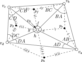
Figure 18: Octahedron $O$ in the half-space model, triangulated according to the construction in Figure 16

Remark.

As Figure 18 indicates, the vertex $p_{h}$ is outside of the triangle $v_{d}v_{a}v_{0}$. As one might expect, formula (8) still applies to the tetrahedron $\{v_{d},v_{a},v_{0},\infty\}$. Since the angle $h$ exceeds $\pi/2$, $\mbox{\cyr L}(h)<0$. So in the formula

$$V(\{v_{d},v_{a},v_{0},\infty\})=\mbox{\cyr L}(AD)+\mbox{\cyr L}(DA)+\mbox{\cyr L}(h),$$

the first two terms correspond to the volumes of the tetrahedra $\{v_{a},v_{0},p_{h},\infty\}$ and $\{v_{0},v_{d},p_{h},\infty\}$, while the last term corresponds to the negative volume of the tetrahedron $\{v_{a},p_{h},v_{d},\infty\}$. Thus one can see how formula (8) still makes geometric as well as analytic sense in the case of a tetrahedron such as $\{v_{d},v_{a},v_{0},\infty\}$.

Looking back at equations (19), (27), and Figure 15, we see that the terms $\mbox{\cyr L}(e)$, $\mbox{\cyr L}(f)$, $\mbox{\cyr L}(g)$, $\mbox{\cyr L}(h)$, which correspond to the tetrahedra $\{v_{a},v_{b},p_{e},\infty\}$, $\{v_{b},v_{c},p_{f},\infty\}$, $\{v_{c},v_{d},p_{g},\infty\}$, $\{v_{d},v_{a},p_{h},\infty\}$ in Figure 18, cancel in the formula for the volume of $T$. Therefore, in our scissors congruence proof we will only be concerned with the tetrahedra

$$\begin{array}[]{cccc}\{v_{0},v_{a},p_{e},\infty\}&\{v_{b},v_{0},p_{e},\infty\}&\{v_{0},v_{b},p_{f},\infty\}&\{v_{c},v_{0},p_{f},\infty\}\\ \{v_{0},v_{c},p_{g},\infty\}&\{v_{d},v_{0},p_{g},\infty\}&\{v_{0},v_{d},p_{h},\infty\}&\{v_{a},v_{0},p_{h},\infty\}\end{array}$$

and their conterparts in $O^{\prime}$. These 8 tetrahedra are shown in Figure 19. They correspond to the first 4 terms in formula (32).

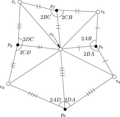
Figure 19: Tetrahedra in the triangulation of the octahedron $O$ that correspond to the first 8 terms in formula (32)

Triangulating $O^{\prime}$ in the same way as $O$ and applying the procedure described in §3.2 and §3.3 to find the unknown dihedral angles, we obtain the polyhedron shown in Figure 20. The tetrahedra shown in that figure correspond to the last 8 terms in formula (32). Thus, up to a multiple of $\pi$, $AB^{\prime}=-\overline{AB}+\arg z_{+}$, $BA^{\prime}=-\overline{BA}-\arg z_{+}$, etc., where $\overline{AB}$, $\overline{BA}$,… are given in (21) and $z_{+}$ is the positive square root solution of (18).

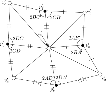
Figure 20: Tetrahedra in the triangulation of the octahedron $O^{\prime}$ that correspond to the last 8 terms in formula (32)

We have found that certain permutations of the tetrahedra in Figure 19 (and corresponding permutations of the tetrahedra in Figure 20) give us new polyhedra that correspond to $R_{b}(T)$ and $R_{c}(T)$. In other words, given that $2T$ is scissors congruent to $O+O^{\prime}$, we have found that $2R_{b}(T)$ is scissors congruent to $P(O)+P(O^{\prime})$, where $P(O)$ and $P(O^{\prime})$ are the octahedra obtained by permuting some of the tetrahedra in the triangulations of $O$ and $O^{\prime}$.

Before stating this fact and its proof formally, we address the fact that there are no permutations of the tetrahedra that give us $R_{a}(T)$. This can be traced back to the choice of the firepole (see Definition 3.1) in triangulating $O$. The firepole, as shown in Figure 10, connects the vertices $a_{2}$ and $a_{2}^{\prime}$. From the position of these vertices in Figure 7, we see that this choice of the firepole “favors” the pair of opposite edges labeled as $A$ and $A^{\prime}$. Similarly, the Regge symmetry $R_{a}$ is singles out the edge with dihedral angle $A$ and its opposite, as seen in Definition 1.1. The other two choices of the firepole for $O$ are the segments $\{b_{1},b_{1}^{\prime}\}$ and $\{c_{1}^{\prime},c_{2}\}$, whose preferred pairs of edges are labeled as $B$, $B^{\prime}$ and $C$, $C^{\prime}$. The first of these choices yields a triangulation of $O$ that admits permutations that correspond to $R_{a}(T)$ and $R_{c}(T)$, while the second allows permutations that give $R_{a}(T)$ and $R_{b}(T)$. In fact, no matter which of the $2^{6}$ possible decomposition one uses to cut down to octahedron, it is always true that for every choice of a firepole that prefers a certain pair of opposite edges one cannot obtain the octahedron corresponding to exactly one of the Regge symmetries $R_{a}$, $R_{b}$ or $R_{c}$ by simply permuting tetrahedra.

The formal statement of the results obtained is as follows.

Theorem 4.1.

Let $T=T(A,B,C,A^{\prime},B^{\prime},C^{\prime})$ be a hyperbolic tetrahedron, and let $R_{b}(T)=T(s_{b}-A,B,s_{b}-C,s_{b}-A^{\prime},B^{\prime},s_{b}-C^{\prime})$ denote the action on $T$ of one of the Regge symmetries, as defined in Definition 1.1. Then $2T$ is scissors congruent to $2R_{b}(T)$.

Proof.

Let $O_{T}$ denote the octahedron obtained from $T$ by the construction in §3, and let $O_{T}^{\prime}$ denote the corresponding dual tetrahedron. As shown in §3.4, $2T$ is scissors congruent to $O_{T}+O_{T}^{\prime}$. We apply the construction described in §3 to $R_{b}(T)$ by first extending its edges to infinity and obtaining the octahedron $U_{R_{b}(T)}$ shown in Figure 21. Then we triangulate $U_{R_{b}(T)}$ so that $O_{R_{b}(T)}$ has as its vertices the points $\{a_{1},b_{1}^{\prime},a_{2}^{\prime},c_{2}^{\prime},b_{2},c_{2}\}$, while $O_{R_{b}(T)}^{\prime}$ has vertices the points $\{a_{2},b_{2}^{\prime},a_{1}^{\prime},c_{1}^{\prime},b_{1},c_{1}\}$. $O_{R_{b}(T)}$ is depicted in Figure 22.

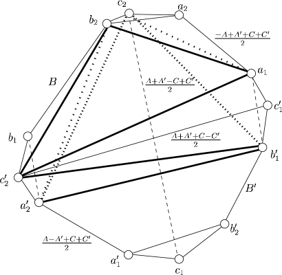
Figure 21: Polyhedron $U_{R_{b}(T)}$

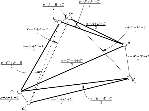
Figure 22: Octahedron $O_{R_{b}(T)}$

Just as in the case of $T$, $2R_{b}(T)$ is scissors congruent to $O_{R_{b}(T)}+O_{R_{b}(T)}^{\prime}$. What remains to be shown is that $O_{T}+O_{T}^{\prime}$ is scissors congruent to $O_{R_{b}(T)}+O_{R_{b}(T)}^{\prime}$. This is done as follows.

Let $O$ be triangulated as shown in Figure 18. We need not consider the tetrahedra $\{v_{a},v_{b},p_{e},\infty\}$, $\{v_{b},v_{c},p_{f},\infty\}$, $\{v_{c},v_{d},p_{g},\infty\}$, and $\{v_{d},v_{a},p_{h},\infty\}$ as they cancel when $O$ is added to $O^{\prime}$. Therefore, it is sufficient to consider the polyhedron shown in Figure 19. The scissors congruence move consists of interchanging the tetrahedra $\{v_{a},p_{e},v_{0},\infty\}$ and $\{v_{0},v_{c},p_{g},\infty\}$, while leaving all the other tetrahedra in place. The resulting polyhedron is shown in Figure 23, where the tetrahedra that were moved are shaded.

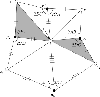
Figure 23: Polyhedron of Figure 19 with the interchanged tetrahedra shown shaded

The pieces in the resulting figure still fit together (i.e. the situation depicted in Figure 12 does not occur) because the new polyhedron satisfies equation (15). In fact, the permutation merely interchanges the terms $\sin(BA)$ and $\sin(DC)$ in (15). As a final step, we translate the 8 tetrahedra making up the polyhedron of Figure 23 to obtain the mirror image of that polyhedron. The result is shown in Figure 24.

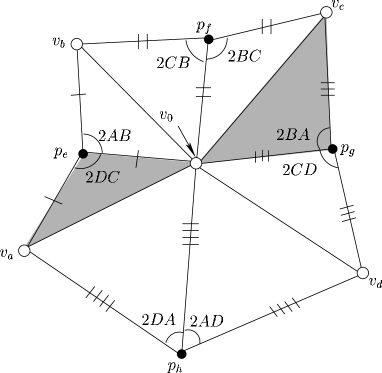
Figure 24: Mirror image of the polyhedron of Figure 23

After adding the tetrahedra $\{v_{b},v_{a},p_{e},\infty\}$, $\{v_{c},v_{b},p_{f},\infty\}$, $\{v_{d},v_{c},p_{g},\infty\}$, and $\{v_{a},v_{d},p_{h},\infty\}$ to the polyhedron in Figure 24 (these tetrahedra will subsequently cancel with their counterparts in $O^{\prime}$) we obtain the octahedron $P(O)$ shown in Figure 25. The dihedral angles in that figure were obtained by adding up the dihedral angles at the edges of the polyhedron in Figure 24, which were given in equations (16), (13) and (21). Clearly, $P(O)$ is isometric to the octahedron $O_{R_{b}(T)}$ in Figure 22.

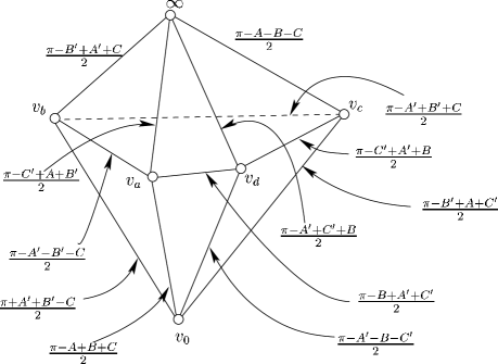
Figure 25: Octahedron $P(O)$ in the Klein model

The discussion above applies verbatim to the dual octahedra. Since their dihedral angles are dependent on the dihedral angles of the original tetrahedra, we need to perform the same permutation on the tetrahedra making up $O^{\prime}$ as we did on the tetrahedra making up $O$. In other words we interchange the tetrahedra $\{v_{a}^{\prime},p_{e}^{\prime},v_{0}^{\prime},\infty\}$ and $\{v_{0}^{\prime},v_{c}^{\prime},p_{g}^{\prime},\infty\}$ in Figure 20 and take the mirror image of the result. We end up with the polyhedron shown in Figure 26.

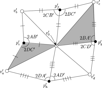
Figure 26: Mirror image of the polyhedron of Figure 20 taken after the shaded tetrahedra have been interchanged

Adding in the tetrahedra $\{v_{b}^{\prime},v_{a}^{\prime},p_{e}^{\prime},\infty\}$, $\{v_{c}^{\prime},v_{b}^{\prime},p_{f}^{\prime},\infty\}$, $\{v_{d}^{\prime},v_{c}^{\prime},p_{g}^{\prime},\infty\}$, and $\{v_{a}^{\prime},v_{d}^{\prime},p_{h}^{\prime},\infty\}$ gives the octahedron shown in Figure 27.

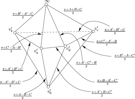
Figure 27: Octahedron $P(O^{\prime})$ in the Klein model

Comparing the octahedra in Figure 25 and Figure 27, we see that their dihedral angles add up to $\pi$. Therefore, the octahedron in Figure 27 is isometric to $O_{R_{b}(T)}^{\prime}$. Thus we have shown that $O+O^{\prime}$ is scissors congruent to $O_{R_{b}(T)}+O_{R_{b}(T)}^{\prime}$ by a permutation. This completes the proof. ∎

Corollary 4.2.

Let $T$ and $R_{b}(T)$ be hyperbolic tetrahedra as defined in Theorem 4.1. Then $T$ is scissors congruent to $R_{b}(T)$.

Proof.

The fact that we can “divide by 2” the construction that led to the proof of Theorem 4.1 follows from Dupont’s result of unique divisibility in [1]. Dupont shows how an ideal hyperbolic tetrahedron can be divided into two parts that are scissors congruent to one another. The fact that this 2-divisibility is unique means that it is well-defined with respect to the different ways to divide a tetrahedron into two scissors congruent sets of polyhedra. In other words, suppose we find that $T=A\coprod B$, where $A$ and $B$ are collections of polyhedra such that $A$ is scissors congruent to $B$. Now suppose that we can also express $T$ as $T=A^{\prime}\coprod B^{\prime}$, where $A^{\prime}$ and $B^{\prime}$ are also scissors congruent to one another. Then by unique 2-divisibility, $A$, $A^{\prime}$, $B$, and $B^{\prime}$ are all scissors congruent to one another.

We saw in the proof of Theorem 4.1 that $2T$ is scissors congruent to $\widetilde{O}+\widetilde{O}^{\prime}$, where $\widetilde{O}$ is the polyhedron in Figure 19 and $\widetilde{O}^{\prime}$ is the polyhedron in Figure 20. We now divide each of the 8 tetrahedra comprising $\widetilde{O}$ into two scissors congruent (in fact, congruent) halves as shown in Figure 28.

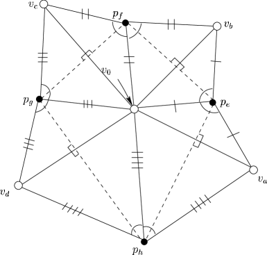
Figure 28: Dividing the polyhedron of Figure 19 into two scissors congruent parts

The result is the polyhedron $\widetilde{O}/2$ shown in Figure 29.

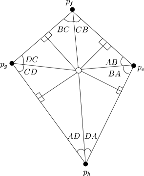
Figure 29: One of the two congruent halves comprising the polyhedron of Figure 19

We perform the same division by 2 procedure on $\widetilde{O}^{\prime}$.

By Dupont’s unique 2-divisibility result, $T$ is scissors congruent to $\widetilde{O}/2+\widetilde{O}^{\prime}/2$, that is to the sum of the polyhedron in Figure 29 and and its dual. Similarly, $R_{b}(T)$ is scissors congruent to $\widetilde{O}_{R_{b}(T)}/2+\widetilde{O}_{R_{b}(T)}^{\prime}/2$. Permuting the indicated tetrahedra in $\widetilde{O}/2$ results in $\widetilde{O}_{R_{b}(T)}/2$, shown in Figure 30. Permuting the corresponding tetrahedra of $\widetilde{O}^{\prime}/2$ results in $\widetilde{O}_{R_{b}(T)}^{\prime}/2$. Since $\widetilde{O}/2+\widetilde{O}^{\prime}/2$ is scissors congruent to $\widetilde{O}_{R_{b}(T)}/2+\widetilde{O}_{R_{b}(T)}^{\prime}/2$ by a permutation of tetrahedra, it follows that $T$ is scissors congruent to $R_{b}(T)$. ∎

Corollary 4.3.

All the tetrahedra in the family generated by the Regge symmetries are scissors congruent to one another.

Proof.

By Theorem 4.1, the tetrahedron $T$ is scissors congruent to $R_{b}(T)$. By applying the construction in the proof of that theorem to the rigid rotations of $T$ we can prove that $T$ is scissors congruent to $R_{a}(T)$ and $R_{c}(T)$. The corrollary then follows from the fact that any two maps out of $R_{a}(T)$, $R_{b}(T)$ and $R_{c}(T)$ generate the group of Regge symmetries, so we can obtain any member of the family of Regge symmetric tetrahedra by a sequence of procedures described in the proof of Theorem 4.1. ∎

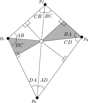
Figure 30: One of the two congruent halves comprising the polyhedron of Figure 24

5 Conclusion

It would be natural at this point to try to extend the result of this paper to spherical simplices. It is not even known with certainty that the Regge symmetry is a scissors congruence in $\mathbb{S}^{3}$, since the conjecture that the volume and Dehn invariant are sufficient invariants for scissors congruence in spherical space is still open. Given the similarities between spherical and hyperbolic spaces, it would certainly be reasonable to hope that the Regge symmetries generate a family of scissors congruent tetrahedra in $\mathbb{S}^{3}$.

Vinberg’s result regarding the analytic continuation of the volume function in [6], §3.1, tells us that Leibon’s volume formulas are valid for spherical tetrahedra up to multiplication by $\pm\sqrt{-1}$. However, the difficulty in applying the construction described above to spherical geometry lies in interpreting these formulas as geometric decompositions. In particular, terms like $\mbox{\cyr L}(\theta)$ can be viewed as halves of the volume of bilaterally symmetric ideal tetrahedra in hyperbolic space. But it is not clear what the analogue of an ideal tetrahedron is in spherical geometry, and so the geometric significance of terms like $\mbox{\cyr L}(\theta)$ is difficult to see.

In Euclidean space, Roberts has already shown in [5] that the Regge symmetry is a scissors congruence, but a constructive proof has not yet been found. Adapting the above described construction to Euclidean space would present a challenge that is in some sense more difficult than the spherical case, since the volume formulas for Euclidean tetrahedra are so different from those for hyperbolic tetrahedra. A successful adaptation of the construction to either spherical or Euclidean tetrahedra would certainly yield many insights into simplices in both of these geometries.

Received:8 October 2002  Revised:22 December 2002

References

- [1] Johan L Dupont, Scissors congruences, group homology and characteristic classes, World Scientific Publishing Company (2001)
- [2] Gregory Leibon, The symmetries of hyperbolic volume, Preprint (2002)
- [3] John Milnor, Hyperbolic geometry: the first 150 years, Bulletin of the American Mathematical Society 6 (1982) 9–24
- [4] Jun Murakami, Masakazu Yano, On the volume of a hyperbolic and spherical tetrahedron, Preprint (2002)
- [5] Justin Roberts, Classical -symbols and the tetrahedron, Geometry and Topology 3 (1999) 21–66
- [6] E B Vinberg, Volumes of non-Euclidean Polyhedra, Russian Mathematical Surveys 48 (1993) 15–45
Received:\qua8 October 2002 Revised:\qua22 December 2002