Modeling Elastic Shells Immersed in Fluid

Abstract.

We describe a numerical method to simulate an elastic shell immersed in a viscous incompressible fluid. The method is developed as an extension of the immersed boundary method using shell equations based on the Kirchhoff-Love and the planar stress hypotheses. A detailed derivation of the shell equations used in the numerical method is presented. This derivation as well as the numerical method, use techniques of differential geometry in an essential way. Our main motivation for the development of this method is its use in the construction of a comprehensive three-dimensional computational model of the cochlea (the inner ear). The central object of study within the cochlea is the “basilar membrane”, which is immersed in fluid and whose elastic properties rather resemble those of a shell. We apply the method to a specific example, which is a prototype of a piece of the basilar membrane and study the convergence of the method in this case. Some typical features of cochlear mechanics are already captured in this simple model. In particular, numerical experiments have shown a traveling wave propagating from the base to the apex of the model shell in response to external excitation in the fluid.

1. Introduction

This paper describes a general method of simulation of an elastic shell immersed in a viscous incompressible fluid. The method is developed as an extension of the immersed boundary method originally introduced by Peskin and McQueen to study the blood flow in the heart. The immersed boundary method has proved to be particularly useful for computer simulation of various biofluid dynamic systems. In this framework the elastic (and possibly active) biological tissue is treated as a collection of elastic fibers immersed in a viscous incompressible fluid. This formulation of the method together with references to many applications can be found in [13]. A partial list of the applications of the immersed boundary method includes in addition to the blood flow in the heart (see the extensive work of Peskin and McQueen, e. g. [14, 10]) also platelet aggregation during blood clotting [4], flow of suspensions [5, 15], aquatic animal locomotion [4], a two-dimensional model of cochlear fluid mechanics [1] and flow in collapsible tubes [3]. For a recent review of the immersed boundary method, see [12].

Many man-made materials can be modeled as elastic shells and elastic shells are also ubiquitous in nature, however our motivation for the development of the method comes from the study of the cochlea. The auditory signal processing in the cochlea depends crucially on the dynamics of the basilar membrane, which is immersed in a viscous incompressible fluid of the cochlea, and despite its name the basilar membrane is actually an elastic shell. The numerical method for elastic shell–fluid interaction presented here was subsequently used in the construction of a complete three-dimensional computational model of the macro-mechanics of the cochlea which incorporates the intricate curved cochlear anatomy. The results of this work will be reported in future publications.

The cochlea is the part of the inner ear where sound waves are transformed into electrical pulses which are carried by neurons to the brain. It is a small snail-shell-like cavity in the temporal bone, which has two openings, the oval window and the round window. The cavity is filled with fluid, which is sealed in by two elastic membranes covering these windows. The spiral canal of the cochlea is divided lengthwise by the long and narrow basilar membrane into two passages that connect with each other at the apex. External sounds set the ear drum in motion, which is conveyed to the inner ear by three small bones of the middle ear. These bones function as an impedance matching device, focusing the energy of the ear drum on the oval window of the cochlea. This piston-like motion against the oval window displaces the fluid of the cochlea generating traveling waves that propagate along the basilar membrane. The vibrations of the basilar membrane are detected by thousands of microscopic sensory receptors, called hair cells, located on the surface of the basilar membrane. The auditory signal processing in the cochlea is completed by the hair cells converting these mechanical stimuli into action potentials in the neurons attached to them, relaying this information to the brain.

Practically everything we know about the passive wave propagation in the cochlea was discovered in the 1940s by Georg von Békésy  who carried out experiments in cochleae extracted from human cadavers. Von Békésy observed that a pure tone input sound generates a traveling wave which reaches its peak at a speciffic location along the basilar membrane   exciting only a narrow band of hair cells. This characteristic location depends on the tone’s frequency. By pinching the basilar membrane with a tiny probe and observing the resulting displacement von Békésy discovered that the basilar membrane is, in fact, not a membrane, i. e. it is not under inner tension, but an elastic shell, whose compliance varies exponentially along the membrane. Von Békésyś extensive experimental work is summarized in his book ”Experiments in Hearing” [16]. For an excellent summary of more recent work on the cochlea, see [6].

Cochlear mechanics has been an active area of research ever since von Békésy’s fundamental contributions, yet many important questions are still open. Presently there is no complete understanding of the mechanisms responsible for the extreme sensitivity, sharp frequency selectivity and broad dynamic range of hearing. The most rigorous mathematical analysis of the cochlea was carried out by Leveque, Peskin and Lax in [9]. In their model the cochlea is represented by a two-dimensional plane (i.e. a strip of infinite length and infinite depth) and the basilar membrane, by a straight line of harmonic oscillators dividing the fluid plane into two halves. The linearized equations are reduced to a functional equation by applying the Fourier transform in the direction parallel to the basilar membrane and then solving the resulting ordinary differential equations in the normal direction. The functional equation derived in this way is solved analytically, and the solution is evaluated both numerically and also asymptotically (by the method of stationary phase). This analysis reveals that the waves in the cochlea resemble shallow water waves, i.e. ripples on the surface of a pond. A distinctive feature of this paper is the (then speculative) consideration of negative basilar membrane friction, i.e., of an amplification mechanism operating within the cochlea.

Like the cochlea, even the simplest three-dimensional fluid–shell systems appear to be too difficult to analyze, but using the methods presented here it is possible to construct computational models for such systems. The construction of computational models for fluid–shell configurations is however not easy, and the development of these methods required supercomputing resources. Nevertheless, with the rapid advances in computer technology, such computations will soon be feasible on a workstation. The cochlea example is important also because the fluid–shell system simulation in this case can be compared with the extensive body of theoretical and experimental research.

The theory of elastic plates and shells is a classical mathematical subject, which is also an active area of contemporary research (see for example [2, 11, 17]). For completeness, we derive in section 2 the elastic shell equations upon which the numerical method is based. Shell theory is very naturally described in the language of differential geometry and it is perhaps in this respect that the presentation in section 2 somewhat differs from other accounts of the subject. Imagine a material composed of very rigid straight line segments (fibers) coupled together and assume that these fibers are perpendicular to some imaginary surface $S$ in the middle of the material. In other words, the material has a structure of a normal vector bundle over the surface $S$. We shall assume that the base surface $S$ is free to undergo arbitrary small elastic deformations. The Kirchhoff-Love hypothesis, is the assumption that the deformation of the bundle is such that the fibers of the deformed bundle are perpendicular to the deformed middle surface, and that these fibers are not stretched during the deformation. In the language of differential geometry this means that the shell has the structure of a normal vector bundle which is preserved under elastic deformations. We shall call such a material an elastic bundle. The Kirchhoff-Love hypothesis implies that a deformation of the base surface completely determines the deformation of the whole bundle. To ensure that the fibers do not intersect each other we must assume that their length, i.e., the thickness of the bundle, is smaller than the radius of maximal curvature of the base surface.

Taking the three-dimensional linear theory of elasticity as our starting point, and using the Kirchhoff-Love hypothesis, it is possible to derive the equations which completely determine small deformations of elastic bundles. It turns out however that a realistic model has to satisfy the hypothesis of planar stress. Strictly speaking, in linear elasticity the planar stress hypothesis is not consistent with the Kirchhoff-Love assumption. We utilize a common approach to “reconciling” the two assumptions (e.g see [7]). The resulting equations constitute a system of three partial differential equations in three unknown functions. They express the elastic force exerted by the shell as a linear fourth order differential operator applied to the displacement vector field. This differential operator is intrinsic to the base surface of the bundle and its coefficients are tensorial quantities determined by the geometry and the elastic properties of the bundle. This intrinsic geometric formulation is essential in the formulation of the numerical method described in the following section.

Section 3 outlines the immersed boundary method for shells. This is a modification of the immersed boundary method as described in [13]. The main difference in the algorithm is in the computation of the force that the material applies to the fluid. Here it is computed by discretizing the shell equations described in section 2. We describe in detail the discrete differential operators defined on the shell surface which are used in the force computation.

In section 4 we describe a test model in which the shell resembles a piece of a basilar membrane immersed in fluid. We study the convergence of the algorithm in this case and describe the numerical experiments carried out with this model. These experiments have reproduced some of the typical features of cochlear mechanics, such as the traveling wave propagating along the basilar membrane in response to external excitation of the fluid.

This work is based on the author’s Ph.D. thesis completed at the Courant Institute (NYU) under the supervision of Professor Charles S. Peskin. I would like to thank Professor Peskin for his support, encouragement and patient guidance. I would also like to thank Professor David McQueen for many conversations in which I learnt a lot about scientific computing. I’d like to thank Professor Karl Grosh for helping me understand shell theory. ‘

2. Linear Elastic Deformations of Vector Bundles (Shell Theory)

Let $M\subset\bf R^{3}$ be a normal bundle over a surface $S$. We describe $S$ by a coordinate chart $\phi:\Omega\to\bf R^{3}$, where $\Omega$ is a domain in $\bf R^{2}$. Let $n:\Omega\to M$ be the unit normal vector field on $S$. The natural chart for $M$ is $\Phi:\Omega\times(-h_{0},h_{0})\to M$ given by

$$\Phi(q_{1},q_{2},t)=\phi(q_{1},q_{2})+tn(q_{1},q_{2}),$$

and we assume, for simplicity, that the thickness of the bundle $(=2h_{0})$ is constant. Let $\Phi_{\epsilon}:\Omega\times(-h_{0},h_{0})\to\bf R^{3}$ describe a 1-parameter family of deformations of $M$, such that $\Phi_{0}=\Phi$. Our basic assumption is that each $\Phi_{\epsilon}$ preserves the bundle structure of $M$. Clearly, such a deformation is completely determined by the deformation of the base space $S$. In the framework of linear elasticity we work with infinitesimal deformations, i.e., vector fields. We will assume that $S$ is free to undergo an arbitrary infinitesimal deformation $\psi=\frac{d}{d\epsilon}|_{\epsilon=0}\phi_{\epsilon}$ and we shall determine the corresponding infinitesimal deformation $V=\frac{d}{d\epsilon}|_{\epsilon=0}\Phi_{\epsilon}$ of $M$.

We begin with some preliminary remarks about the geometry of $M$. Throughout this chapter the indices are raised and lowered with respect to $h$, the metric of $S$. We adopt the convention that greek indices take the values $1,2$, while roman indices run through $1,2,3$. The standard metric on $\bf R^{3}$ will be denoted by $\delta$:

$$\delta(X,Y)=<X,Y>=X\cdot Y,$$

$\partial_{\alpha}=\frac{\partial}{\partial q_{\alpha}}$ is a partial derivative and $\overline{\nabla}$ is the standard flat connection of $\bf R^{3}$.

2.1. The Geometry of the Vector Bundle

Let $h=\phi^{\ast}\left(\delta|_{S}\right)$ denote the metric of $S$ in the chart $\phi$. The components of $h$ are

$$h_{\alpha\beta}=\partial_{\alpha}\phi\cdot\partial_{\beta}\phi.$$

Throughout this paper greek tensor indices are raised and lowered with respect to the metric $h$. Let $N_{p}$ denote the unit normal vector to $S$ at the point $p\in M$. Thus, $n(q_{1},q_{2})=N_{\phi(q_{1},q_{2})}$. We shall often abuse notation and identify $n$ with $N$. Similarly for other vector fields. The second fundamental form of $S$ is the symmetric bilinear form acting on vectors tangent to the surface $S$ defined by

$$b(X,Y)=<{\overline{\nabla}}_{X}N,Y>.$$

Its components in the chart $\phi$ are

$$b_{\alpha\beta}=\partial_{\alpha}n\cdot\partial_{\beta}\phi.$$

The central role in the following analysis is played by the map $\theta=\theta_{t}$, which we define to be the flow of $N$:

$$\theta_{t}(p)=p+t\,N_{p},\ \ \ \ \,p\in S.$$

The differential of $\theta$ is the map

$$\theta_{\ast}:T_{p}S\to T_{\theta(p)}S_{t},$$

where $S_{t}=\theta_{t}(S)$. Let $X\in T_{p}S$ and let $\sigma$ be a curve on $S$ such that $\sigma(0)=p$, $\sigma^{\prime}(0)=X$. Then

$$\theta_{\ast}X = \theta_{\ast}\sigma^{\prime}$$

$$= (\theta\circ\sigma)^{\prime}$$

$$= (\sigma+t\,N\circ\sigma)^{\prime}$$

$$= X+t\,{\overline{\nabla}}_{X}N$$

We shall regard $\theta_{\ast}$ as a symmetric tensor field on $S$. The components $\theta_{\alpha\beta}$ of $\theta_{\ast}$ can be expressed in the chart $\phi$ as follows:

(1) $$\theta_{\alpha\beta} = <\theta_{\ast}(\partial_{\alpha}\phi),\,\partial_{\beta}\phi>$$

$$= <\partial_{\alpha}\phi+t\,{\overline{\nabla}}_{\partial_{\alpha}\phi}N,\,\partial_{\beta}\phi>$$

$$= \partial_{\alpha}\phi\cdot\partial_{\beta}\phi+t\,\partial_{\alpha}n\cdot\partial_{\beta}\phi$$

$$= h_{\alpha\beta}+t\,b_{\alpha\beta}.$$

An important observation which will be useful later is:

(2) $${\overline{\nabla}}_{X}N={\overline{\nabla}}_{\theta_{\ast}X}N$$

for any tangent vector $X$. Indeed, let $\tilde{\sigma}=\theta\circ\sigma$. Then $\theta_{\ast}X=\tilde{\sigma}^{\prime}$ and

$${\overline{\nabla}}_{\theta_{\ast}X}N = {\overline{\nabla}}_{\tilde{\sigma}^{\prime}}N$$

$$= \lim_{\epsilon\to 0}\frac{N(\tilde{\sigma}(\epsilon))-N(\tilde{\sigma}(0))}{\epsilon}$$

$$= \lim_{\epsilon\to 0}\frac{N(\sigma(\epsilon))-N(\sigma(0))}{\epsilon}$$

$$= {\overline{\nabla}}_{X}N$$

We denote the metric of $M$ in the chart $\Phi$ by ${\rm g}$. Its components, $\mbox{${\rm g}$}_{ij}=\partial_{i}\Phi\cdot\partial_{j}\Phi$, are

$$\mbox{${\rm g}$}_{\alpha\beta} = \theta_{\alpha}{}^{\sigma}\theta_{\sigma\beta}$$

$$\mbox{${\rm g}$}_{3\alpha} = 0$$

$$\mbox{${\rm g}$}_{33} = 1$$

The collection of parallel surfaces $S_{t}$ forms a foliation of $M$. This foliation carries the induced connection $\nabla$ given by

$$\nabla_{X}Y={\overline{\nabla}}_{X}Y-<{\overline{\nabla}}_{X}Y,\,N>N$$

for any two vector fields $X$ and $Y$ which are tangent to the foliation. The second fundamental form of this foliation is the symmetric bilinear form acting on tangent vectors defined by

$$B(X,Y)=<{\overline{\nabla}}_{X}N,\,Y>.$$

Thus

$$\nabla_{X}Y={\overline{\nabla}}_{X}Y+B(X,Y)N.$$

The components of $B$ in the chart $\Phi$ are

(3) $$B_{\alpha\beta} = (\Phi^{\ast}B)(\partial_{\alpha},\partial_{\beta})$$

$$= B(\partial_{\alpha}\Phi,\partial_{\beta}\Phi)$$

$$= <{\overline{\nabla}}_{\partial_{\alpha}\Phi}N,\partial_{\beta}\Phi>$$

$$= <{\overline{\nabla}}_{\theta_{\ast}(\partial_{\alpha}\phi)}N,\partial_{\beta}\Phi>$$

$$= <{\overline{\nabla}}_{\partial_{\alpha}\phi}N,\partial_{\beta}\Phi>$$

$$= \partial_{\alpha}n\cdot(\theta_{\beta}{}^{\sigma}\partial_{\sigma}\phi)$$

$$= b_{\alpha\sigma}\theta_{\beta}{}^{\sigma}$$

$$= \theta_{\alpha}{}^{\sigma}b_{\sigma\beta}.$$

The map $\theta$ plays an important role because it allows us to extend any tensor $A$ on the base surface $S$ to a tensor $\theta_{\ast}A$ on the whole bundle $M$.

We conclude the description of the geometry of $M$ with its volume element $dv$. It can be decomposed as follows

$$dv=dA_{t}\,dt,$$

where $dA_{t}$ is the area element of $S_{t}$. Since $S_{t}=\theta(S)$, we have

$$dA_{t}=\det(\theta_{\ast})\,dA_{0}.$$

Notice than in $\bf R^{3}$

$$\det(\theta_{\ast}) = \det(h+tb)$$

$$= 1+({\rm tr}\,b)\,t+(\det\,b)\,t^{2}$$

$$= 1+H\,t+K\,t^{2},$$

where $H$ and $K$ denote the mean curvature and the Gaussian curvature of the surface $S$ respectively.

2.2. The Infinitesimal Deformation of an Elastic Bundle

We shall assume that the deformation field of the base surface $S$ is given by

$$\psi=\omega\,N+W,$$

where $W=W^{\sigma}\partial_{\sigma}\phi$ is an arbitrary vector field tangent to $S$ and $\omega$ is an arbitrary function on $S$. We extend $\omega$ to the whole bundle $M$ by the normal flow, but we’ll continue to write $\omega$ instead of $\theta_{\ast}\omega=\omega\circ\theta$. In this section we will show that the corresponding deformation vector field of the elastic bundle $M$ is given by

(4) $$V=\omega\,N+\theta_{\ast}W-t\,T^{\left(\omega\right)}\,,$$

where

$$T^{\left(\omega\right)}(q_{1},q_{2},t)=T^{\left(\omega\right)}(q_{1},q_{2})=h^{\mu\nu}\,\partial_{\mu}\omega\,\partial_{\nu}\phi.$$

From the assumption that the deformations should preserve the bundle structure it follows that $\Phi_{\epsilon}$ has the following form:

$$\Phi_{\epsilon}=\phi_{\epsilon}+t\,n_{\epsilon}\,,$$

where $\phi_{\epsilon}$ is a coordinate system for the deformed base space and $n_{\epsilon}$ is the normal to it. We have $\phi_{0}=\phi$, $n_{0}=n$ and

(5) $$V = \left.{\frac{d}{d\epsilon}}\right|_{\epsilon=0}\Phi_{\epsilon}$$

$$= \psi+t\,\left.{\frac{d}{d\epsilon}}\right|_{\epsilon=0}n_{\epsilon}\,.$$

On one hand

(6) $$\left(\left.{\frac{d}{d\epsilon}}\right|_{\epsilon=0}n_{\epsilon}\right)\cdot n=\frac{1}{2}\,\left.{\frac{d}{d\epsilon}}\right|_{\epsilon=0}(n_{\epsilon}\cdot n_{\epsilon})=0\,,$$

while on the other hand

(7) $$\left(\left.{\frac{d}{d\epsilon}}\right|_{\epsilon=0}n_{\epsilon}\right)\cdot\partial_{\alpha}\phi = \left.{\frac{d}{d\epsilon}}\right|_{\epsilon=0}(n_{\epsilon}\cdot\partial_{\alpha}\phi_{\epsilon})-n\cdot\left.{\frac{d}{d\epsilon}}\right|_{\epsilon=0}\partial_{\alpha}\phi_{\epsilon}$$

$$= -n\cdot\partial_{\alpha}\psi$$

$$= -\partial_{\alpha}(\psi\cdot n)+\psi\cdot\partial_{\alpha}n$$

$$= -\partial_{\alpha}\omega+\psi\cdot b_{\alpha}{}^{\sigma}\partial_{\sigma}\phi$$

$$= -\partial_{\alpha}\omega+b_{\alpha}{}^{\sigma}W_{\sigma}\,.$$

Using (6) and (7) in (5) we have

$$V = \omega\,N+W+t\,(-\partial_{\alpha}\omega+b_{\alpha}{}^{\sigma}\,W_{\sigma})\,h^{\alpha\tau}\,\partial_{\tau}\phi$$

$$= \omega\,N+(h_{\alpha}{}^{\sigma}+t\,b_{\alpha}{}^{\sigma})\,W_{\sigma}\,h^{\alpha\tau}\,\partial_{\tau}\phi-t\,\partial_{\alpha}\omega\,h^{\alpha\tau}\,\partial_{\tau}\phi$$

$$= \omega\,N+\theta_{\alpha}{}^{\sigma}\,W_{\sigma}\,h^{\alpha\tau}\,\partial_{\tau}\phi-t\,\partial_{\alpha}\omega\,h^{\alpha\tau}\,\partial_{\tau}\phi$$

$$= \omega\,N+\theta_{\ast}W-t\,T^{\left(\omega\right)}\,,$$

which is what was claimed in (4).

2.3. The Strain Tensor

Let $\overline{g}=\delta|_{M}$ be the metric of the bundle $M$. The strain tensor corresponding to the deformation vector field $V$ is the symmetric tensor $e$ defined by

$$e=\frac{1}{2}{\cal L}_{V}\overline{g},$$

the Lie derivative of $\overline{g}$ in the direction of $V$. We now show that for any tangent vector field $X$,

(8) $$e(X,N)=0.$$

Let $g_{\epsilon}=\Phi^{\ast}_{\epsilon}(\overline{g})$ be the metric of the deformed bundle in the chart $\Phi_{\epsilon}$. Its components are:

$$(g_{\epsilon})_{ij}=\partial_{i}\Phi_{\epsilon}\cdot\partial_{j}\Phi_{\epsilon}.$$

The components of the strain tensor in the chart $\Phi$ are

$$e_{ij}=\frac{1}{2}\left.{\frac{d}{d\epsilon}}\right|_{\epsilon=0}\left(\partial_{i}\Phi_{\epsilon}\cdot\partial_{j}\Phi_{\epsilon}\right)$$

We have

(9) $$e_{33} = \partial_{3}\Phi\cdot\left.{\frac{d}{d\epsilon}}\right|_{\epsilon=0}\partial_{3}\Phi_{\epsilon}$$

$$= n\cdot\left.{\frac{d}{d\epsilon}}\right|_{\epsilon=0}n_{\epsilon}$$

$$= 0$$

and

(10) $$e_{3\alpha} = \frac{1}{2}\left.{\frac{d}{d\epsilon}}\right|_{\epsilon=0}\left(n_{\epsilon}\cdot\partial_{\alpha}\phi_{\epsilon}+t\,n_{\epsilon}\cdot\partial_{\alpha}n_{\epsilon}\right)$$

$$= \frac{1}{2}\left(-(\partial_{\tau}\psi\cdot n)h^{\tau\sigma}\partial_{\sigma}\phi\cdot\partial_{\alpha}\phi+n\cdot\partial_{\alpha}\psi\right)$$

$$= 0,$$

which shows (8). We can now express the strain tensor in terms of the function $\omega$ and the vector field $W$:

$$e = \frac{1}{2}{\cal L}_{V}\,\overline{g}$$

$$= \frac{1}{2}{\cal L}_{\omega N+\theta_{\ast}W-t\,T^{\left(\omega\right)}}\,\overline{g}$$

$$= \frac{1}{2}{\cal L}_{\omega N}\,\overline{g}+\widehat{\nabla(\theta_{\ast}W)}-t\,\widehat{\nabla T^{\left(\omega\right)}}.$$

Here $\hat{A}$ stands for the symmetrization of A:

$$\hat{A}_{\mu\nu}=\frac{1}{2}(A_{\mu\nu}+A_{\nu\mu}).$$

For tangential fields $X$, $Y$ we have

$${\cal L}_{\omega N}\,\overline{g}(X,Y)=\omega\,N<X,Y>-<{\cal L}_{\omega N}X,Y>-<X,{\cal L}_{\omega N}Y>.$$

Since

$${\cal L}_{\omega N}X = \omega NX-X(\omega N)$$

$$= \omega{\cal L}_{N}X-(X\omega)N$$

we have

$$<{\cal L}_{\omega N}X,Y>=\omega<{\cal L}_{N}X,Y>$$

and

$${\cal L}_{\omega N}\overline{g}(X,Y)=\omega{\cal L}_{N}\overline{g}(X,Y).$$

Finally the strain tensor is given by

(11) $$e=\omega B+\widehat{\nabla(\theta_{\ast}W)}-t\,\widehat{\nabla T^{\left(\omega\right)}}.$$

For future reference we obtain the expressions for the components of the tensors $\nabla T^{\left(\omega\right)}$ and $\nabla(\theta_{\ast}W)$ in the chart $\Phi$:

(12) $$\nabla_{\alpha}T^{\left(\omega\right)}_{\beta} = \nabla T^{\left(\omega\right)}(\partial_{\alpha}\Phi,\,\partial_{\beta}\Phi)$$

$$= \theta_{\alpha}{}^{\sigma}\theta_{\beta}{}^{\tau}\nabla T^{\left(\omega\right)}(\partial_{\sigma}\phi,\,\partial_{\tau}\phi)$$

$$= \theta_{\alpha}{}^{\sigma}\theta_{\beta}{}^{\tau}<\nabla_{\partial_{\sigma}\phi}T^{\left(\omega\right)},\,\partial_{\tau}\phi>$$

$$= \theta_{\alpha}{}^{\sigma}\theta_{\beta}{}^{\tau}<{\overline{\nabla}}_{\partial_{\sigma}\phi}T^{\left(\omega\right)},\,\partial_{\tau}\phi>$$

$$= \theta_{\alpha}{}^{\sigma}\theta_{\beta}{}^{\tau}\partial_{\sigma}T^{\left(\omega\right)}\cdot\partial_{\tau}\phi$$

$$= \theta_{\alpha}{}^{\sigma}\theta_{\beta}{}^{\tau}\nabla_{\sigma}\nabla_{\tau}\omega,$$

where $\nabla_{\sigma}\nabla_{\tau}\omega$ are the components of the Hessian of $\omega$ on $S$ in the chart $\phi$, and

(13) $$\nabla(\theta_{\ast}W)_{\alpha\beta} = <\nabla_{\partial_{\alpha}\Phi}(\theta_{\ast}W),\,\partial_{\beta}\Phi>$$

$$= \theta_{\alpha}{}^{\sigma}\theta_{\beta}{}^{\tau}<\nabla_{\partial_{\sigma}\phi}(\theta_{\ast}W),\,\partial_{\tau}\phi>$$

$$= \theta_{\alpha}{}^{\sigma}\theta_{\beta}{}^{\tau}<\nabla_{\partial_{\sigma}\phi}(W^{\mu}\theta_{\mu}{}^{\nu}\partial_{\nu}\phi),\,\partial_{\tau}\phi>$$

$$= \theta_{\alpha}{}^{\sigma}\theta_{\beta}{}^{\tau}\nabla_{\sigma}(W^{\mu}\theta_{\mu\tau})$$

$$= \theta_{\alpha}{}^{\sigma}\theta_{\beta}{}^{\tau}\theta_{\tau\mu}(\nabla_{\sigma}W^{\mu})+\theta_{\alpha}{}^{\sigma}\theta_{\beta}{}^{\tau}(\nabla_{\sigma}\theta_{\mu\tau})W^{\mu}$$

Substituting (12) and (13) in (11) we obtain

(14) $$e_{\alpha\beta}=B_{\alpha\beta}\,\omega\,-\,t\,\theta_{\alpha}{}^{\sigma}\theta_{\beta}{}^{\tau}\,\nabla_{\sigma}\nabla_{\tau}\omega\,+\,\theta_{\alpha}{}^{\sigma}\mbox{${\rm g}$}_{\beta}{}^{\tau}\,(\nabla_{\sigma}W_{\tau})\,+\,\theta_{\alpha}{}^{\sigma}\theta_{\beta}{}^{\tau}(\nabla_{\sigma}\theta_{\tau}{}^{\mu})\,W_{\mu}\,.$$

2.4. The Plane Stress Assumption.

In linear elasticity the stress tensor $\sigma$ is related to the strain tensor $e$ by the generalized Hooke’s law:

$$\sigma^{ij}=C^{ijkl}e_{kl}$$

where

$$C_{ijkl}=C_{ijkl}(q_{1},q_{2},t)$$

denote the components of the elasticity 4-tensor $C$ in the chart $\Phi$. For a homogeneous and isotropic material the elasticity tensor is of the form

(15) $$C^{ijkl}=\lambda\,\mbox{${\rm g}$}^{ij}\mbox{${\rm g}$}^{kl}+\mu\,\mbox{${\rm g}$}^{ik}\mbox{${\rm g}$}^{jl}+\mu\,\mbox{${\rm g}$}^{il}\mbox{${\rm g}$}^{jk}\,.$$

In this case Hooke’s law of linear elasticity takes the form

(16) $$\sigma_{ij}=\lambda\,\mbox{${\rm g}$}^{mn}e_{mn}\,\mbox{${\rm g}$}_{ij}+2\mu\,e_{ij}=\lambda\,{\rm tr}(e)\,\mbox{${\rm g}$}_{ij}+2\mu\,e_{ij}\,.$$

The strain energy corresponding to the strain $e$ is defined by

$${\cal E}=\frac{1}{2}\int_{M}C(e,e)\,dv=\frac{1}{2}\int_{M}C^{ijkl}e_{ij}e_{kl}$$

It is now possible to derive a shell theory based solely on the Kirchhoff-Love hypothesis using the expression for the strain tensor (14). It turns out however that a more realistic shell model is obtained using the assumption of plane stress:

(17) $$\sigma_{33}=0.$$

In linear elasticity this assumption contradicts the Kirchhoff-Love hypothesis. We follow a standard approach in modifying the Kirchhoff-Love hypothesis (see [7]): we no longer assume that

$$e_{33}=0,$$

but we continue to assume that

$$e_{3\alpha}=0.$$

Let $\overline{e}$ denote the tangential part of the strain $e$. From (16) and (17) it follows that

$$0=\sigma_{33}=\lambda\mbox{${\rm g}$}^{mn}e_{mn}+2\mu e_{33}=\lambda\mbox{${\rm g}$}^{\mu\nu}e_{\mu\nu}+(\lambda+2\mu)e_{33}$$

and therefore

$$e_{33}=-\frac{\lambda}{\lambda+2\mu}\mbox{${\rm g}$}^{\mu\nu}e_{\mu\nu}=-\frac{\lambda}{\lambda+2\mu}tr\overline{e}\,.$$

We use the last equation to simplify the expression for the strain energy:

$$C(e,e)=\lambda\,(g^{mn}e_{mn})^{2}+2\mu\,g^{mn}g^{kj}\,e_{mj}e_{kn}=\lambda({\rm tr}e)^{2}+2\mu{\rm tr}(e^{2})\,.$$

Since

$${\rm tr}e={\rm tr}\overline{e}+e_{33}=(1-\frac{\lambda}{\lambda+2\mu})~{}{\rm tr}\overline{e}=\frac{2\mu}{\lambda+2\mu}~{}{\rm tr}\overline{e}$$

and

$${\rm tr}(e^{2})={\rm tr}(\overline{e}^{2})+e_{33}^{2}={\rm tr}(\overline{e}^{2})+\frac{\lambda^{2}}{(\lambda+2\mu)^{2}}({\rm tr}\overline{e})^{2}$$

we obtain

$$C(e,e) = 4\lambda\frac{\mu^{2}}{(\lambda+2\mu)^{2}}({\rm tr}\overline{e})^{2}+2\mu\frac{\lambda^{2}}{(\lambda+2\mu)^{2}}({\rm tr}\overline{e})^{2}+2\mu{\rm tr}(\overline{e}^{2})$$

$$= \frac{2\lambda\mu}{\lambda+2\mu}({\rm tr}\overline{e})^{2}+2\mu{\rm tr}(\overline{e}^{2})\,.$$

2.5. Variation of the Strain Energy

In order to obtain the equilibrium equations we proceed to calculate the variation of the strain energy. Let $\tilde{\omega}$ be an arbitrary function and $\tilde{W}$ an arbitrary vector field on $S$. The corresponding variation of the energy is

$$\delta{\cal E}=\lim_{\epsilon\to 0}\frac{{\cal E}(\omega+\epsilon\tilde{\omega},W+\epsilon\tilde{W})-{\cal E}(\omega,W)}{\epsilon}\,.$$

Let $\tilde{e}=\overline{e}(\tilde{V})$ be the strain corresponding to the deformation $\tilde{V}$. Since

$$\overline{e}(V+\tilde{V})=\overline{e}(V)+\overline{e}(\tilde{V})$$

the variation of the strain energy is

$$\delta{\cal E} = \frac{\lambda\mu}{\lambda+2\mu}\,\int_{M}{\rm tr}\overline{e}~{}{\rm tr}\tilde{e}\,dv+\mu\int_{M}{\rm tr}(\overline{e}\,\tilde{e})\,dv$$

$$= \int_{\Omega}\int_{-h_{0}}^{h_{0}}\left(\frac{\lambda\mu}{\lambda+2\mu}\,\mbox{${\rm g}$}^{\alpha\beta}\mbox{${\rm g}$}^{\gamma\delta}+\mu\,\mbox{${\rm g}$}^{\alpha\gamma}\mbox{${\rm g}$}^{\beta\delta}\right)e_{\alpha\beta}\tilde{e}_{\gamma\delta}\,\det(\theta_{\ast})\,dt\,dA_{0}$$

$$= \int_{\Omega}\int_{-h_{0}}^{h_{0}}\Lambda^{\alpha\beta\gamma\delta}e_{\alpha\beta}\tilde{e}_{\gamma\delta}\,dt\,dA_{0},$$

where we define

$$\Lambda^{\alpha\beta\gamma\delta}(q_{1},q_{2},t)=\left(\frac{\lambda\mu}{\lambda+2\mu}\,\mbox{${\rm g}$}^{\alpha\beta}\mbox{${\rm g}$}^{\gamma\delta}+\mu\,\mbox{${\rm g}$}^{\alpha\gamma}\mbox{${\rm g}$}^{\beta\delta}\right)\,\det(\theta_{\ast})\,.$$

For the calculations that follow it is useful to note the following symmetries of $\Lambda$:

$$\Lambda^{\alpha\beta\gamma\delta}=\Lambda^{\beta\alpha\gamma\delta}=\Lambda^{\alpha\beta\delta\gamma}=\Lambda^{\gamma\delta\alpha\beta}\,.$$

We use (14) and integrate by parts omitting the boundary terms to rewrite the energy variation as follows

$$\delta{\cal E} = \int_{\Omega}\int_{-h_{0}}^{h_{0}}\Lambda^{\alpha\beta\gamma\delta}e_{\alpha\beta}\left(B_{\gamma\delta}\tilde{\omega}-t\,\theta_{\gamma}{}^{\sigma}\theta_{\delta}{}^{\tau}\nabla_{\sigma}\nabla_{\tau}\tilde{\omega}+\theta_{\gamma}{}^{\sigma}\mbox{${\rm g}$}_{\delta}{}^{\tau}\nabla_{\sigma}\tilde{W}_{\tau}+\theta_{\gamma}{}^{\sigma}\theta_{\delta}{}^{\tau}\nabla_{\sigma}\theta_{\tau}{}^{\mu}\tilde{W}_{\mu}\right)\,dt\,dA_{0},$$

$$= \int_{\Omega}\int_{-h_{0}}^{h_{0}}\left(\Lambda^{\alpha\beta\gamma\delta}e_{\alpha\beta}B_{\gamma\delta}-t\,\nabla_{\tau}\nabla_{\sigma}\left(\Lambda^{\alpha\beta\gamma\delta}e_{\alpha\beta}\theta_{\gamma}{}^{\sigma}\theta_{\delta}{}^{\tau}\right)\right)\,\tilde{\omega}\,dt\,dA_{0},$$

$$\mbox{}+\int_{\Omega}\int_{-h_{0}}^{h_{0}}\left(\Lambda^{\alpha\beta\gamma\delta}e_{\alpha\beta}\theta_{\gamma}{}^{\sigma}\theta_{\delta}{}^{\tau}\nabla_{\sigma}\theta_{\tau}{}^{\mu}-\nabla_{\sigma}\left(\Lambda^{\alpha\beta\gamma\delta}e_{\alpha\beta}\theta_{\gamma}{}^{\sigma}\mbox{${\rm g}$}_{\delta}{}^{\mu}\right)\right)\tilde{W}_{\mu}\,dt\,dA_{0},$$

Collecting the terms we obtain the equations for the normal and the tangential components of the force

$$f^{3} = \int_{-h_{0}}^{h_{0}}\left(\Lambda^{\alpha\beta\gamma\delta}e_{\alpha\beta}B_{\gamma\delta}-t\,\nabla_{\tau}\nabla_{\sigma}\left(\Lambda^{\alpha\beta\gamma\delta}e_{\alpha\beta}\theta_{\gamma}{}^{\sigma}\theta_{\delta}{}^{\tau}\right)\right)\,dt$$

$$f^{\mu} = \int_{-h_{0}}^{h_{0}}\left(\Lambda^{\alpha\beta\gamma\delta}e_{\alpha\beta}\theta_{\gamma}{}^{\sigma}\theta_{\delta}{}^{\tau}\nabla_{\sigma}\theta_{\tau}{}^{\mu}-\nabla_{\sigma}\left(\Lambda^{\alpha\beta\gamma\delta}e_{\alpha\beta}\theta_{\gamma}{}^{\sigma}\mbox{${\rm g}$}_{\delta}{}^{\mu}\right)\right)\,dt$$

Using (14) again we can finally bring these equations into the following form

$$f^{3} = A\,\omega+\nabla_{\sigma}\nabla_{\tau}(\overline{A}^{\sigma\tau\mu\nu}\nabla_{\mu}\nabla_{\nu}\omega)-\nabla_{\sigma}\nabla_{\tau}(\overline{\overline{A}}^{\sigma\tau}\omega)-\overline{\overline{A}}^{\sigma\tau}\nabla_{\sigma}\nabla_{\tau}\omega$$

$$\mbox{}+\Phi^{\nu}W_{\nu}+\overline{\Phi}^{\mu\nu}\nabla_{\mu}W_{\nu}-\nabla_{\sigma}\nabla_{\tau}(\Psi^{\mu\sigma\tau}W_{\mu})-\nabla_{\mu}\nabla_{\nu}(\overline{\Psi}^{\sigma\tau\mu\nu}\nabla_{\sigma}W_{\tau})$$

$$f^{\mu} = \Omega^{\mu\nu}\,W_{\nu}+\overline{\Omega}^{\sigma\tau\mu}\,\nabla_{\sigma}W_{\tau}-\nabla_{\sigma}(\overline{\Omega}^{\sigma\mu\tau}W_{\tau})-\nabla_{\nu}(\overline{\overline{\Omega}}^{\sigma\tau\nu\mu}\nabla_{\sigma}W_{\tau})$$

$$\mbox{}+\Phi^{\mu}\,\omega-\nabla_{\nu}(\overline{\Phi}^{\nu\mu}\,\omega)-\Psi^{\mu\sigma\tau}\nabla_{\sigma}\nabla_{\tau}\omega+\nabla_{\nu}(\overline{\Psi}^{\nu\mu\sigma\tau}\nabla_{\sigma}\nabla_{\tau}\omega)$$

where the coefficients are defined as follows:

(20) $$A = \int\Lambda^{\alpha\beta\gamma\delta}B_{\alpha\beta}B_{\gamma\delta}\,dt$$

(21) $$\overline{A}^{\sigma\tau\mu\nu} = \int\Lambda^{\alpha\beta\gamma\delta}\theta_{\alpha}{}^{\sigma}\theta_{\beta}{}^{\tau}\theta_{\gamma}{}^{\mu}\theta_{\delta}{}^{\nu}\,t^{2}\,dt$$

(22) $$\overline{\overline{A}}^{\mu\nu} = \int\Lambda^{\alpha\beta\gamma\delta}B_{\alpha\beta}\theta_{\gamma}{}^{\mu}\theta_{\delta}{}^{\nu}\,t\,dt$$

$$\Phi^{\mu} = \int\Lambda^{\alpha\beta\gamma\delta}B_{\alpha\beta}\theta_{\gamma}{}^{\tau}\theta_{\delta}{}^{\rho}(\nabla_{\tau}\theta_{\rho}{}^{\mu})\,dt$$

$$= \overline{\overline{A}}^{\tau\rho}\nabla_{\tau}b_{\rho}{}^{\mu}$$

(24) $$\overline{\Phi}^{\mu\nu} = \int\Lambda^{\alpha\beta\gamma\delta}B_{\alpha\beta}\theta_{\gamma}{}^{\mu}\theta_{\delta}{}^{\tau}\theta_{\tau}{}^{\nu}\,dt$$

$$\Psi^{\rho\mu\nu} = \int\Lambda^{\alpha\beta\gamma\delta}\theta_{\alpha}{}^{\sigma}\theta_{\beta}{}^{\tau}(\nabla_{\sigma}\theta_{\tau}{}^{\rho})\theta_{\gamma}{}^{\mu}\theta_{\delta}{}^{\nu}\,t\,dt$$

$$= \overline{A}^{\sigma\tau\mu\nu}\nabla_{\sigma}b_{\tau}{}^{\rho}$$

(26) $$\overline{\Psi}^{\sigma\tau\mu\nu} = \int\Lambda^{\alpha\beta\gamma\delta}\theta_{\alpha}{}^{\sigma}\mbox{${\rm g}$}_{\beta}{}^{\tau}\theta_{\gamma}{}^{\mu}\theta_{\delta}{}^{\nu}\,t\,dt$$

$$\Omega^{\mu\nu} = \int\Lambda^{\alpha\beta\gamma\delta}\theta_{\alpha}{}^{\sigma}\theta_{\beta}{}^{\tau}(\nabla_{\sigma}\theta_{\tau}{}^{\mu})\theta_{\gamma}{}^{\lambda}\theta_{\delta}{}^{\rho}(\nabla_{\lambda}\theta_{\rho}{}^{\nu})\,dt$$

$$= \overline{A}^{\sigma\tau\lambda\rho}\nabla_{\sigma}b_{\tau}{}^{\mu}\nabla_{\lambda}b_{\rho}{}^{\nu}$$

$$\overline{\Omega}^{\mu\nu\rho} = \int\Lambda^{\alpha\beta\gamma\delta}\theta_{\alpha}{}^{\mu}\mbox{${\rm g}$}_{\beta}{}^{\nu}\theta_{\gamma}{}^{\tau}\theta_{\delta}{}^{\lambda}(\nabla_{\tau}\theta_{\lambda}{}^{\rho})\,dt$$

$$= \overline{\Psi}^{\sigma\tau\mu\nu}\nabla_{\nu}b_{\mu}{}^{\rho}$$

(29) $$\overline{\overline{\Omega}}^{\sigma\tau\mu\nu} = \int\Lambda^{\alpha\beta\gamma\delta}\theta_{\alpha}{}^{\sigma}\mbox{${\rm g}$}_{\beta}{}^{\tau}\theta_{\gamma}{}^{\mu}\mbox{${\rm g}$}_{\delta}{}^{\nu}\,dt$$

2.6. The Plate Equation

For a flat shell surface $S$ the only non-zero coefficients are $\overline{A}$ and $\overline{\overline{\Omega}}$ ($\overline{\Psi}$ is zero because it is an integral of an odd function on a symmetric interval), and

$$\Lambda^{\sigma\tau\mu\nu} = \frac{\lambda\mu}{\lambda+2\mu}h^{\sigma\tau}h^{\mu\nu}+\mu h^{\sigma\mu}h^{\tau\nu}$$

$$\overline{A}^{\sigma\tau\mu\nu} = \frac{2}{3}h_{0}^{3}\,\Lambda^{\sigma\tau\mu\nu}$$

$$\overline{\overline{\Omega}}^{\sigma\tau\mu\nu} = 2h_{0}\,\Lambda^{\sigma\tau\mu\nu}$$

The equations (2.5) – (2.5) reduce to

$$f_{normal} = \frac{2}{3}h_{0}^{3}D\,\Delta^{2}\omega$$

$$f_{tangential} = 2h_{0}D\,\nabla\div W$$

where

$$D=2\mu\frac{\lambda+\mu}{\lambda+2\mu}\,.$$

The first equation is the classical equation of an elastic plate (see [8]). The second equation does not appear in classical plate analysis where it is assumed that the plate undergoes only vertical motion and the shearing forces are negligible.

3. The Immersed Boundary Method

The immersed boundary method of Peskin and McQueen is a general numerical method for modeling an elastic material immersed in a viscous incompressible fluid. Typically the immersed material has been modeled as a collection of fibers. For details and references to many applications see [13] and [12]. This section outlines the immersed boundary method with the elastic material being modeled as a shell.

3.1. The Equations of the Model

For the description of the fluid we adopt a standard cartesian coordinate system on $\bf R^{3}$. The immersed material is described in a different curvilinear coordinate system. The equations can be partitioned into three groups: the Navier Stokes equations of a viscous incompressible fluid, the equations describing the elastic material and the interaction equations. Accordingly there are two distinct computational grids: one for the fluid and the other for the immersed material. The purpose of the interaction equations is to communicate between these two grids.

We first turn to the Navier-Stokes equations. Let $\rho$ and $\mu$ denote the density and the viscosity of the fluid, and let ${{\bf u}}({{\bf x}},t)$ and $p({{\bf x}},t)$ denote its velocity and pressure, respectively. Then

(30) $$\rho\left(\frac{\partial{\bf u}}{\partial t}+{\bf u}\cdot\nabla{\bf u}\right) = \mbox{}-\nabla p+\mu\nabla^{2}{\bf u}+{\bf F}$$

(31) $$\nabla\cdot{\bf u} = 0$$

where ${\bf F}$ denotes the density of the body force acting on the fluid. For example, if the immersed material is modeled as a thin shell, then ${\bf F}$ is a singular vector field, which is zero everywhere, except possibly on the surface representing the shell.

Let ${\bf X}({\bf q},t)$ denote the position of the immersed material in $\bf R^{3}$. For a shell, ${\bf q}$ takes values in a domain $\Omega\subset\bf R^{2}$, and ${\bf X}({\bf q},t)$ is a 1-parameter family of surfaces indexed by $t$, i.e., ${\bf X}({\bf q},t)$ is the middle surface of the shell at time $t$. Let ${\bf f}({\bf q},t)$ denote the force density that the immersed material applies on the fluid. Then

(32) $${\bf F}({\bf x},t)=\int{\bf f}({\bf q},t)\delta({\bf x}-{\bf X}({\bf q},t))\,d{\bf q},$$

where $\delta$ is the Dirac delta function on $\bf R^{3}$. This equation merely says that the fluid feels the force that the material exerts on it, but it is important in the numerical method where it is one of the interaction equations mentioned above. The other interaction equation is the no slip condition for a viscous fluid:

(33) $$\frac{\partial{\bf X}}{\partial t} = {\bf u}({\bf X}({\bf q},t),t)$$

$$= \int{\bf u}({\bf x},t)\delta({\bf x}-{\bf X}({\bf q},t))\,d{\bf x}$$

We will now complete the description of the system by writing down the third group of equations, the equations describing the shell. Let ${\bf X}_{0}({\bf q})$ denote the initial position, which we take as our equilibrium reference configuration, of the middle surface of the shell, and let ${\bf T}_{\mu}={\bf T}_{\mu}({\bf q})=\frac{\partial}{\partial q_{\mu}}$ ($\mu=1,2$) be its tangent coordinate vector fields. The displacement from the stationary configuration can be described in terms of the function $\omega({\bf q},t)$ and the vector field ${\bf W}({\bf q},t)$ defined by the following equation:

$${\bf X}({\bf q},t)-{\bf X}_{0}({\bf q})=\omega({\bf q},t){\bf N}({\bf q})+{\bf W}({\bf q},t),$$

where ${\bf N}={\bf N}({\bf q})$ denotes the normal to the surface ${\bf X}_{0}({\bf q})$ and ${\bf W}=W^{\mu}{\bf T}_{\mu}$ is tangent to ${\bf X}_{0}$. We decompose the force ${\bf f}$ into its normal and tangential components as well:

$${\bf f}=f^{3}{\bf N}+f^{\mu}{\bf T}_{\mu}$$

The components $f^{i}$ are related to $\omega$ and $W^{\mu}$ by the shell equations (2.5) – (2.5). This completes the description of the fluid-shell system.

3.2. The Numerical Method

Let ${\Delta t}$ denote the duration of a time step. It will be convenient to denote the time step by the superscript. For example ${\bf u}^{n}({\bf x})={\bf u}({\bf x},n{\Delta t}).$ At the beginning of the $n$-th time step ${\bf X}^{n}$ and ${\bf u}^{n}$ are known. Each time step proceeds as follows.

1. Compute the force ${\bf f}^{n}$ that the shell applies to the fluid.

2. Use (32) to compute the external force on the fluid ${\bf F}^{n}$.

3. Compute the new fluid velocity ${\bf u}^{n+1}$ from the Navier Stokes equations.

4. Use (33) to compute the new position ${\bf X}^{n+1}$ of the immersed material.

The computation of the force in step 1 is explained in detail in the next section. We shall now describe in detail the computations in steps 2 — 4, beginning with the Navier-Stokes equations.

The fluid equations are discretized on a rectangular lattice of mesh width $h$. We will make use of the following difference operators which act on functions defined on this lattice:

(34) $${D^{+}_{i}}\phi({\bf x}) = \frac{\phi({\bf x}+h{\bf e}_{i})-\phi({\bf x})}{h}$$

(35) $${D^{-}_{i}}\phi({\bf x}) = \frac{\phi({\bf x})-\phi({\bf x}-h{\bf e}_{i})}{h}$$

(36) $${D^{0}_{i}}\phi({\bf x}) = \frac{\phi({\bf x}+h{\bf e}_{i})-\phi({\bf x}-h{\bf e}_{i})}{2h}$$

(37) $${\bf D^{0}} = (D^{0}_{1},D^{0}_{2},D^{0}_{3})$$

where $i=1,2,3$, and ${\bf e}_{1}$, ${\bf e}_{2}$, ${\bf e}_{3}$ form an orthonormal basis of $\bf R^{3}$.

In step 3 we use the already known ${\bf u}^{n}$ and ${\bf F}^{n}$ to compute ${\bf u}^{n+1}$ and $p^{n+1}$ by solving the following linear system of equations:

(38) $$\rho\left(\frac{{\bf u}^{n+1}-{\bf u}^{n}}{\Delta t}+\sum_{k=1}^{3}u_{k}^{n}D_{k}^{\pm}{\bf u}^{n}\right) = \mbox{}-{\bf D}^{0}p^{n+1}+\mu\sum_{k=1}^{3}D^{+}_{k}D^{-}_{k}{\bf u}^{n+1}+{\bf F}^{n}$$

(39) $${\bf D}^{0}\cdot{\bf u}^{n+1} = 0$$

Here $u_{k}^{n}D_{k}^{\pm}$ stands for upwind differencing:

$$u_{k}^{n}D_{k}^{\pm}=\left\{\begin{array}[]{ll}u_{k}^{n}D_{k}^{-}&u_{k}^{n}>0\\ u_{k}^{n}D_{k}^{+}&u_{k}^{n}<0\end{array}\right.$$

Equations (38) – (39) are linear constant coefficient difference equations and, therefore, can be solved efficiently with the use of the Fast Fourier Transform algorithm.

We now turn to the discretization of equations (32), (33). Let us assume, for simplicity, that $\Omega\subset\bf R^{2}$ is a rectangular domain over which all of the quantities related to the shell are defined. We will assume that this domain is discretized with mesh widths $\Delta q_{1}$, $\Delta q_{2}$ and the computational lattice for $\Omega$ is the set

$${\bf Q}=\left\{(i_{1}\Delta q_{1},i_{2}\Delta q_{2})\ |\ i_{1}=1\ldots n_{1},\ \ i_{2}=1\ldots n_{2}\right\}.$$

In step 2 the force ${\bf F}^{n}$ is computed using the following equation.

(40) $${\bf F}^{n}({\bf x})=\sum_{{\bf q}\in{\bf Q}}{\bf f}^{n}({\bf q})\delta_{h}({\bf x}-{\bf X}^{n}({\bf q}))\Delta{\bf q}$$

where $\Delta{\bf q}=\Delta q_{1}\Delta q_{2}$ and $\delta_{h}$ is a smoothed approximation to the Dirac delta function on $\bf R^{3}$ described below.

Similarly, in step 4 updating the position of the immersed material ${\bf X}^{n+1}$ is done using the equation

(41) $${\bf X}^{n+1}({\bf q})={\bf X}^{n}({\bf q})+\Delta t\sum_{\bf x}{\bf u}^{n+1}({\bf x})\delta_{h}({\bf x}-{\bf X}^{n}({\bf q}))h^{3}\,,$$

where the summation is over the lattice ${\bf x}=(hi,hj,hk)$, where $i$, $j$ and $k$ are integers.

The function $\delta_{h}$ which is used in (40) and (41), is defined as follows:

$$\delta_{h}({\bf x})=h^{-3}\phi(\frac{x_{1}}{h})\phi(\frac{x_{2}}{h})\phi(\frac{x_{3}}{h})\,,$$

where

$$\phi(r)=\left\{\begin{array}[]{cl}\frac{1}{8}(3-2|r|+\sqrt{1+4|r|-4r^{2}})&|r|\leq 1\\ \frac{1}{2}-\phi(2-|r|)&1\leq|r|\leq 2\\ 0&2\leq|r|\end{array}\right.$$

For an explanation of the construction of $\delta_{h}$ see [13].

3.3. Computation of the Elastic Force

The force ${\bf f}^{n}$, that the shell applies to the fluid is computed by discretizing equations (2.5) – (2.5). We shall now describe how to discretize these equations and how to compute various geometric quantities, such as the Christoffel symbols, the second fundamental form, etc. These basic geometric quantities, as well as the coefficients (20) – (29) that depend on them, can be computed once in the initialization step of the algorithm and stored for subsequent use.

A covariant derivative of a $(p,q)$-tensor $A$ is defined by

(42) $$\nabla_{\alpha}A_{\mu_{1}\ldots\mu_{p}}^{\nu_{1}\ldots\nu_{q}}=\partial_{\alpha}A_{\mu_{1}\ldots\mu_{p}}^{\nu_{1}\ldots\nu_{q}}+\sum_{k=1}^{q}\Gamma_{\alpha\sigma}^{\nu_{k}}A_{\mu_{1}\ldots\mu_{p}}^{\nu_{1}\ldots\sigma\ldots\nu_{q}}-\sum_{m=1}^{p}\Gamma_{\alpha\mu_{m}}^{\sigma}A_{\mu_{1}\ldots\sigma\ldots\mu_{p}}^{\nu_{1}\ldots\nu_{q}}\,,$$

where

$$\Gamma^{\lambda}_{\mu\nu}=\frac{1}{2}g^{\lambda\sigma}\left(g_{\mu\sigma,\nu}+g_{\sigma\nu,\mu}-g_{\mu\nu,\sigma}\right)$$

are the Christoffel symbols, $g_{\mu\nu}={\bf T}_{\mu}\cdot{\bf T}_{\nu}$ is the metric of the surface ${\bf X}_{0}$, $g^{\mu\nu}$ is the inverse of $g_{\mu\nu}$, and comma denotes partial differentiation (i.e., $\phi_{,\alpha}=\partial_{\alpha}\phi$). To simplify the discretization of the force equations we introduce a single difference operator $D_{\alpha}$ which uses center differencing in the interior of the domain and either forward or backward differencing on the boundary:

$$D_{\alpha}\phi({\bf q})=\left\{\begin{array}[]{ll}D^{+}_{\alpha}\phi({\bf q})&q_{\alpha}=\Delta q_{\alpha}\\ D^{0}_{\alpha}\phi({\bf q})&2\Delta q_{\alpha}\leq q_{\alpha}\leq(n_{\alpha}-1)\Delta q_{\alpha}\\ D^{-}_{\alpha}\phi({\bf q})&q_{\alpha}=n_{\alpha}\Delta q_{\alpha}\end{array}\right.$$

Here the operators $D^{+}_{\alpha}$, $D^{0}_{\alpha}$ and $D^{-}_{\alpha}$ are defined on the lattice ${\bf Q}$ analogously to the definitions (34) – (37). We define the discrete covariant derivative of a $(p,q)$-tensor $A$ by

(43) $$\tilde{D}_{\alpha}A_{\mu_{1}\ldots\mu_{p}}^{\nu_{1}\ldots\nu_{q}}=D_{\alpha}A_{\mu_{1}\ldots\mu_{p}}^{\nu_{1}\ldots\nu_{q}}+\sum_{k=1}^{q}\Gamma_{\alpha\sigma}^{\nu_{k}}A_{\mu_{1}\ldots\mu_{p}}^{\nu_{1}\ldots\sigma\ldots\nu_{q}}-\sum_{m=1}^{p}\Gamma_{\alpha\mu_{m}}^{\sigma}A_{\mu_{1}\ldots\sigma\ldots\mu_{p}}^{\nu_{1}\ldots\nu_{q}}\,.$$

The following computations are carried out in the initialization stage of the algorithm:

1. Compute the tangent vector fields ${\bf T}_{\alpha}=D_{\alpha}{\bf X}_{0}$.

2. Compute the unit normal vector field ${\bf N}=\frac{{\bf T}_{1}\times{\bf T}_{2}}{\left|{\bf T}_{1}\times{\bf T}_{2}\right|}\,.$

3. Compute the metric $g_{\mu\nu}={\bf T}_{\mu}\cdot{\bf T}_{\nu}$ and its inverse $g^{\mu\nu}$.

4. Compute the second fundamental form: $b_{\mu\nu}=D_{\mu}{\bf N}\cdot{\bf T}_{\nu}$ .

5. Compute the Christoffel symbols:

   $$\Gamma^{\lambda}_{\mu\nu}=\frac{1}{2}g^{\sigma\lambda}(D_{\nu}g_{\mu\sigma}+D_{\mu}g_{\sigma\nu}-D_{\sigma}g_{\mu\nu})\,.$$

6. Compute the derivative of the second fundamental form:

   $$\tilde{D}_{\alpha}b_{\beta}{}^{\gamma}=D_{\alpha}b_{\beta}{}^{\gamma}+\Gamma_{\alpha\sigma}^{\gamma}b_{\beta}{}^{\sigma}-\Gamma_{\alpha\beta}^{\sigma}b_{\sigma}{}^{\gamma}\,.$$

7. Compute the coefficients (20) – (29). In practice instead of evaluating the integrals in these expressions it is easier to assume that the shell is sufficiently thin and to drop the terms involving high powers of the thickness.

The computation of the force during each time step proceeds as follows:

1. Decompose the displacement into its tangential and normal components:

   $$\omega=({\bf X}^{n}-{\bf X}_{0})\cdot{\bf N}$$

   $$W_{\alpha}=({\bf X}^{n}-{\bf X}_{0})\cdot{\bf T}_{\alpha}$$

2. Compute $D_{\mu}\omega$, the components of $d\omega$, the 1-form dual to the gradient of $\omega$.

3. Compute $\tilde{D}_{\mu}D_{\nu}\omega$, the components of the hessian of $\omega$.

4. Compute the components $\tilde{D}_{\mu}W_{\nu}$.

5. Compute the normal and the tangential components of the force using the following discretization of the equations (2.5) - (2.5):

   (44) $$f^{3} = A\,\omega+\tilde{D}_{\sigma}\tilde{D}_{\tau}(\overline{A}^{\sigma\tau\mu\nu}\tilde{D}_{\mu}D_{\nu}\omega)-\tilde{D}_{\sigma}\tilde{D}_{\tau}(\overline{\overline{A}}^{\sigma\tau}\omega)-\overline{\overline{A}}^{\sigma\tau}\tilde{D}_{\sigma}D_{\tau}\omega$$

   $$\mbox{}+\Phi^{\nu}W_{\nu}+\overline{\Phi}^{\mu\nu}\tilde{D}_{\mu}W_{\nu}-\tilde{D}_{\sigma}\tilde{D}_{\tau}(\Psi^{\mu\sigma\tau}W_{\mu})-\tilde{D}_{\mu}\tilde{D}_{\nu}(\overline{\Psi}^{\sigma\tau\mu\nu}\tilde{D}_{\sigma}W_{\tau})$$

   (45) $$f^{\mu} = \Omega^{\mu\nu}\,W_{\nu}+\overline{\Omega}^{\sigma\tau\mu}\,\tilde{D}_{\sigma}W_{\tau}-\tilde{D}_{\sigma}(\overline{\Omega}^{\sigma\mu\tau}W_{\tau})-\tilde{D}_{\nu}(\overline{\overline{\Omega}}^{\sigma\tau\nu\mu}\tilde{D}_{\sigma}W_{\tau})$$

   $$\mbox{}+\Phi^{\mu}\,\omega-\tilde{D}_{\nu}(\overline{\Phi}^{\nu\mu}\,\omega)-\Psi^{\mu\sigma\tau}\tilde{D}_{\sigma}D_{\tau}\omega+\tilde{D}_{\nu}(\overline{\Psi}^{\nu\mu\sigma\tau}\tilde{D}_{\sigma}D_{\tau}\omega)$$

To complete the computation, we express the force in cartesian coordinates using

$${\bf f}=f^{3}{\bf N}+f^{\mu}{\bf T}_{\mu}.$$

4. An Application: Modeling a Shell Immersed in Fluid

In this chapter we present a model shell which is a prototype of a piece of the basilar membrane of the cochlea. The immersed boundary method for shells was implemented using the C programming language and numerical experiments were carried out with this shell. We describe the model that was used, examine the convergence of the algorithm in this case and discuss the results.

4.1. The Model Shell

We construct a shell similar to a piece of the basilar membrane. Our shell will be approximately one seventh of the length of the basilar membrane in the human cochlea and it will have more curvature. Introducing more curvature allows us to pack a longer shell into a cube of fluid of a given size. Choosing a small fluid cube enables us to achieve a better numerical resolution of the fluid.

The surface is a narrow helicoidal strip defined as follows. Consider the curve

$$\gamma(t)=(R\cos(\alpha t),R\sin(\alpha t),H\alpha t)$$

where $R$, $\alpha$ and $H$ are constants. They are specified, along with the other parameters that we use below, in Table 1.

Table 1. Parameters of the numerical test model

$a=0.1$ cm	length of the side of the fluid cube
$N=32,64,128$	size of the fluid grid is $N^{3}$
$h=\frac{a}{N}$	fluid mesh width
$\rho=1.034$ cm g-3	fluid density
$\nu=0.0197$ g cm-1 sec-1	fluid viscosity
$L_{BM}=3.5$ cm	length of the basilar membrane
$L=0.5$ cm	length of the model shell
$w_{0}=0.015$ cm	width of the basilar membrane at the base
$w_{1}=0.056$ cm	width of the basilar membrane at the apex
$w(q_{1})=w_{0}+\frac{q_{1}}{L_{BM}}(w_{1}-w_{0})$	width of the model shell
$h(q_{1})\approx 0.001(1.0+5.0~{}q_{1})$ cm	thickness of the model shell
$\alpha=1.8\pi/L$
$R=\frac{1}{30}$ cm
$H=0.01$ cm
$n_{1}=1280\frac{N}{128}$	first dimension of the surface grid
$n_{2}=48\frac{N}{128}$	second dimension of the surface grid
$\Delta q_{1}=\frac{L}{n_{1}-1}$	surface mesh width
$\Delta q_{2}(q_{1})=\frac{w(q_{1})}{n_{2}-1}$	surface mesh width
$\lambda=26197503.0$ g cm-1 sec-2	first Lamé coefficient
$\mu=523950.0$ g cm-1 sec-2	second Lamé coefficient
$\Delta t=0.5,~{}1.0,~{}2.0,~{}4.0\times 10^{-8}$ sec	time step
$T_{0}=2.0\times 10^{-6}$ sec	total simulation time

The vector field

$$N(t)=(-\cos(\alpha t),-\sin(\alpha t),0)$$

is a unit normal field along the curve $\gamma$. We define the surface of the shell by the following equation:

$${\bf X}(q_{1},q_{2}) = \gamma(q_{1})+\left(q_{2}-\frac{w(q_{1})}{2}\right)N(q_{1}),$$

$$0\leq q_{1}\leq L,\qquad\frac{-w(q_{1})}{2}\leq q_{2}\leq\frac{w(q_{1})}{2}$$

The width $w$ is chosen to grow linearly, similar to the width of the basilar membrane (see Table 1). This surface is discretized on a grid of size $n_{1}\times n_{2}$ as follows:

$${\bf X}_{k_{1},k_{2}} = \gamma(k_{1}\Delta q_{1})+\left(k_{2}\,\Delta q_{2}(k_{1}\Delta q_{1})-\frac{w(k_{1}\Delta q_{1})}{2}\right)N(k_{1}\Delta q_{1})$$

$$\qquad k_{1}=1,...,n_{1},\qquad k_{2}=1,...,n_{2}.$$

The compliance of an elastic shell is defined as the amount of volume displaced per unit pressure difference across the shell. Von Bekesy found that the compliance per unit length of the basilar membrane varies exponentially along the basilar membrane as $e^{cq_{1}}$, where $c^{-1}=0.7$ cm (see [16]). To achieve this compliance in the model shell we use the shell equations to estimate the required thickness. (Notice that nothing changes in the derivation of the shell equations when the thickness $h_{0}$ is assumed to be a function on the middle surface, rather than being a constant. The thickness enters the equations only in the definition of the coefficients (20) – (29)). We obtain an estimated thickness

$$h(q_{1})=0.001~{}\left(1+\frac{2}{3}q_{1}\right)^{\frac{5}{3}}10^{-\frac{2}{9}q_{1}}\textrm{ cm,}$$

which on the interval $0\leq q_{1}\leq 0.5$ is very close to a straight line (Figure 1).

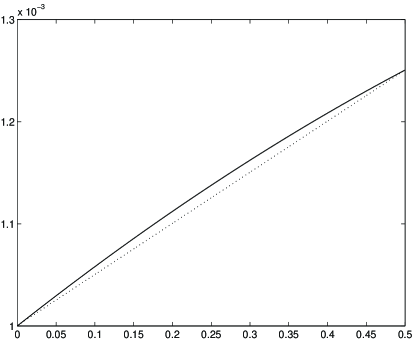
Figure 1. The thickness of the model shell.

The above choices of the width, the thickness and the Láme coefficients (see Table 1) yield an estimated compliance similar to the one measured by von Bekesy for the basilar membrane.

4.2. The Numerical Experiments

The immersed boundary method for shells was implemented using the C programming language. The program ran on the Cray C-90 at the Pittsburgh Supercomputing Center as well as on Silicon Graphics workstations.

The numerical experiments are set up as follows. The shell ${\bf X}$ is placed in a periodic cube of fluid, i.e., a three-dimensional torus. The length of this cube’s side is $a=0.1$ cm, so it is much smaller than the cochlea, whose volume is approximately 1 cm³. The fluid density $\rho$, and the fluid viscosity $\nu$, are chosen equal to the corresponding parameters of the cochlear fluid. The fluid equations are discretized on a cubic grid of $N^{3}$ points and the grid size for the shell is chosen correspondingly such that its mesh widths, $\Delta q_{1}$ and $\Delta q_{2}$, are approximately equal to half of the fluid mesh width $h$ (Table 1). This choice is necessary to prevent the fluid from leaking through the shell. The edges of the shell’s boundary are clamped to a fixed location in space with two rows of springs along each edge.

At time 0 the system is perturbed with a force impulse in the fluid and the simulation is run for a fixed period of time $T_{0}=2.0\times 10^{-6}$ sec. The force impulse acting at time 0 is represented by a constant singular vector field in the vertical direction defined on the horizontal plane $z=0.1~{}\mbox{cm}$ (where $z$ is the vertical coordinate) with the force density of $4\times 10^{-7}~{}\mbox{g cm}^{-1}\mbox{sec}^{-2}$. Since the force source is broadly distributed through a horizontal plane within the fluid, wave propagation within the basilar membrane can only arise as a consequence of its material properties and cannot be the result of the location of the force source.

Immersed boundary computations typically require large scale computing resources. Because of time and storage limitations, it is not possible to conduct an extensive empirical study of the algorithm’s convergence. At present it is not practical to implement the method with a fluid grid of more than $128^{3}$ points. The experiment has been repeated with $N=32,64\textrm{ and }128$ and time steps $\Delta t=0.5,~{}1.0,~{}2.0\textrm{ and }4.0\times 10^{-8}$ sec. Numerical stability condition forces a choice of such small time steps. On the other hand, reducing the time step further may result in a significant machine precision error.

4.3. Convergence of the Algorithm

Let ${\bf X}_{1}(t)$ and ${\bf X}_{2}(t)$ denote the position of the shell at time $t$ obtained in two different numerical experiments. To measure the relative difference at time $t$ we calculate

(46) $$E(t)=\frac{|{\bf X}_{1}(t)-{\bf X}_{2}(t)|_{p}}{|{\bf X}_{1}(t)-{\bf X}_{1}(0)|_{p}}$$

where the norms are $L^{p}$-norms with $p=1,2\textrm{ and }\infty$.

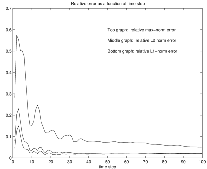
Figure 2. The relative difference between ${\bf X}_{1,128}$ and ${\bf X}_{2,128}$.

For any two experiments the function $E$ has been found to decrease initially very sharply, stabilizing in the second half of the time interval. Two typical graphs are shown in Figure 2 and Figure 3. Therefore, we will measure the difference between two computed solutions on the time interval $[\frac{T_{0}}{2},~{}T_{0}]$ using the following space-time norms:

$$\|{\bf X}_{1}-{\bf X}_{2}\|_{p}=\sum_{t\in[0.5~{}T_{0},~{}T_{0}]}|{\bf X}_{1}(t)-{\bf X}_{2}(t)|_{p}$$

where the summation is taken over the set of 25 time values common to all of the tests performed and the $L^{p}$-norms are computed on the “common” grid of $257\times 12$ points.

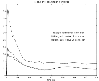
Figure 3. The relative difference between ${\bf X}_{0.5,128}$ and ${\bf X}_{0.5,64}$.

The computations were performed with double precision floating point on a Silicon Graphics computer. The results of the measurements are summarized in Table 2 and Table 3. These results indicate that the algorithm converges when the time step $\Delta t$ is linearly proportional to the mesh width $h$ and both tend to zero.

Table 2. Norm comparison between different numerical tests.

Tests compared			$L^{1}$-norm	$L^{2}$-norm	$L^{\infty}$-norm
1.0/128	–	2.0/64	$9.6290\times 10^{-08}$	$1.8547\times 10^{-09}$	$9.7749\times 10^{-11}$
2.0/64	–	4.0/32	$2.3984\times 10^{-07}$	$4.6353\times 10^{-09}$	$1.8326\times 10^{-10}$
0.5/128	–	1.0/64	$9.2989\times 10^{-08}$	$1.8086\times 10^{-09}$	$9.5158\times 10^{-11}$
1.0/64	–	2.0/32	$2.4082\times 10^{-07}$	$4.7011\times 10^{-09}$	$1.9287\times 10^{-10}$

Let ${\bf X}_{\delta,\overline{N}}$ denote the position of the shell computed with $\Delta t=\delta\times 10^{-8}$ and $N=\overline{N}$. Using the data in Table 2 we have two estimates of the order of convergence of the algorithm:

$$r_{1}=\log_{2}\left(\frac{\|{\bf X}_{1,128}-{\bf X}_{2,64}\|_{p}}{\|{\bf X}_{2,64}-{\bf X}_{4,32}\|_{p}}\right)$$

and

$$r_{2}=\log_{2}\left(\frac{\|{\bf X}_{0.5,128}-{\bf X}_{1,64}\|_{p}}{\|{\bf X}_{1,64}-{\bf X}_{2,32}\|_{p}}\right)$$

The values of $r_{1}$ and $r_{2}$ are given in Table 3. As the time step becomes smaller, the machine precision error becomes more significant leading to a slower rate of convergence. This is apparently the reason that we have $r_{2}<r_{1}$.

Table 3. Convergence rate estimates.

	$L^{1}$-norm	$L^{2}$-norm	$L^{\infty}$-norm
$r_{1}$	1.3729	1.3781	1.0192
$r_{2}$	1.3166	1.3215	0.9068

4.4. The Traveling Wave

The test model described above was run with $N=128$ and time step $\Delta t=1.0\times 10^{-8}$ seconds for a total of more than 2400 time steps. Although this model is still far from a realistic model of the cochlea, several qualitative features, characteristic of the cochlear wave mechanics, were already observed in this experiment.

In the experiment a traveling wave is produced in response to the force impulse in the fluid. The wave propagates in the direction of increasing compliance within the elastic shell. This agrees with von Békésy’s observation that the traveling wave in the cochlea always propagates from the base to the apex (see [16]). Snapshots of this wave are shown in Figure 4. The ten snapshots were taken every 200 time steps beginning with time step 600. The first five appear in the first column, the rest in the second. Since the displacements of the shell are too small to be seen with the naked eye, they are represented in the pictures on a gray scale. Black color indicates the maximal possible displacement down, and white, the maximal displacement up (the scale is symmetric with respect to zero). The initial force impulse has pushed the fluid down and, as can be seen from the first snapshot, after 600 time steps the shell is displaced downwards. In the following snapshots we can see that the stiffer part of the shell near the base is bouncing back and a wave starts propagating towards the apex.

$\begin{array}[]{c@{\hspace{0.1in}}c}\vspace{-3cm}\epsfbox{s6.ps}\hfil\hskip 7.22743pt&\epsfbox{s16.ps}\\ \vspace{-3cm}\epsfbox{s8.ps}\hfil\hskip 7.22743pt&\epsfbox{s18.ps}\\ \vspace{-3cm}\epsfbox{s10.ps}\hfil\hskip 7.22743pt&\epsfbox{s20.ps}\\ \vspace{-3cm}\epsfbox{s12.ps}\hfil\hskip 7.22743pt&\epsfbox{s22.ps}\\ \vspace{-3cm}\epsfbox{s14.ps}\hfil\hskip 7.22743pt&\epsfbox{s24.ps}\\ \end{array}$

Figure 4. The traveling wave in the test shell.

Conclusion and Further Research

This paper describes an extension of the immersed boundary method to elastic shells in a viscous incompressible fluid. The method was developed as a part of a project to construct a three-dimensional computational model of the cochlea. It is based on shell equations derived using techniques of differential geometry. The resulting method is a practical method which has been implemented and tested on a prototype of a piece of the basilar membrane. We have examined the convergence of the algorithm in this case. Numerical experiments indicate that the algorithm has the first order convergence rate when the time step is chosen to be linearly proportional to the fluid mesh width.

The numerical experiments have shown a traveling wave propagating in the test model shell in the direction of increasing material compliance in response to external impulsive excitation of the fluid. This reproduces the so-called “travelling wave paradox” observed in the cochlea: the traveling wave always travels from the base to the apex of the cochlea independently of the location of the impulse source.

The numerical method described here was subsequently used in a construction of a complete three-dimensional computational model of the macro-mechanics of the cochlea. Additional difficulties in the construction of this model are caused by the large scale of the immersed boundary computations required, and by the presence in the fluid of several different elastic materials in addition to the basilar membrane. The size of a human cochlea is on the order of 1 cm $\times$ 1 cm $\times$ 1 cm, while the basilar membrane is about 3.6 cm long and is very narrow (150—560 $\mu$m). Therefore, larger fluid grid is necessary in the full cochlea simulation in order to resolve the 100 $\mu$m scale corresponding to the width of the basilar membrane. Immersed boundary computations require large scale computing resources: a fluid grid of $256\times 256\times 128$ points needed for the full cochlea model requires a significant amount of computer memory. The CFL condition and the stability conditions imposed by the stiffness forces of the immersed boundaries force a choice of a very small time step (approximately 50 nano-seconds) when the fluid mesh width is small. The convergence study carried out in this paper indicates that decreasing the fluid mesh width by a factor of two necessitates a corresponding decrease in the time step by approximately a factor of two. This has indeed been further verified in the construction of the complete cochlea model.

The construction of the cochlea model has been achieved in collaboration with Julian Bunn on Hewlett-Packard computers at the Center for Advanced Computational Research at Caltech. The results of this work will be described in future publications.

References

- [1] R. P. Beyer. A computational model of the cochlea using the immersed boundary method. J. Comp. Phys., 98:145–162, 1992.
- [2] P. G. Ciarlet. Introduction to Linear Shell Theory. Gauthier-Villars, Paris, 1998.
- [3] Rosar M. E. and Peskin C. S. Fluid flow in collapsible elastic tubes: a three-dimensional numerical model. New York J. Math., 7:281–302, 2001.
- [4] L. J. Fauci and A. L. Fogelson. Truncated newton method and modeling of complex immersed elastic structures. Comm. Pure Appld. Math., 46:787–818, 1993.
- [5] A. L. Fogelson and C. S. Peskin. A fast numerical method for solving the three-dimensional stokes’ equations in the presence of suspended particles. J. Comp. Phys., 79:50–69, 1988.
- [6] C. D. Geisler. From Sound to Synapse. Oxford University Press, New York, 1998.
- [7] T. J. R. Hughes. The Finite Element Method–Linear Static and Dynamic Finite Element Analysis. Dover Publishers, 2000.
- [8] A. Leissa. Vibration of Plates. Acoustical Society of America, 1993.
- [9] R. J. Leveque, C. S. Peskin, and P. D. Lax. Solution of a two-dimensional cochlea model with fluid viscosity. SIAM J. Appl. Math., 48:191–213, 1988.
- [10] D. M. McQueen and C. S. Peskin. Heart simulation by an immersed boundary method with formal second-order accuracy and reduced numerical viscosity. In H. Aref and J.W. Phillips, editors, Proceedings of the International Conference on Theoretical and Applied Mechanics (ICTAM) 2000. Kluwer Academic Publishers, 2001.
- [11] F. I. Niordson. Shell theory. North Holland, 1985.
- [12] C. S. Peskin. The immersed boundary method. Acta Numerica, 11:479–517, 2002.
- [13] C. S. Peskin and D. M. McQueen. A general method for the computer simulation of biological systems interacting with fluids. In Proc. of SEB Symposium on Biological Fluid Dynamics, Leeds, England,, July 1994.
- [14] C. S. Peskin and D. M. McQueen. Fluid dynamics of the heart and its valves. In Hans G. Othmer, Fred R. Adler, Mark A. Lewis, and John C. Dallon, editors, Case Studies in Mathematical Modeling – Ecology, Physiology and Cell Biology, pages 309–338. Prentice-Hall, Upper Saddle River, NJ, 1997.
- [15] D. Sulsky and J. U. Brackbill. A numerical method for suspension flow. J. Comp. Phys., 96:339–368, 1991.
- [16] G. von Békésy. Experiments in Hearing. Mc-Graw Hill, New York, 1960.
- [17] I. I. Vorovich. Nonlinear Theory of Shallow Shells. Springer-Verlag, New York, 1999.