A route to computational chaos revisited: noninvertibility and the breakup of an invariant circle

Abstract

In a one-parameter study of a noninvertible family of maps of the plane arising in the context of a numerical integration scheme, Lorenz studied a sequence of transitions from an attracting fixed point to “computational chaos.” As part of the transition sequence, he proposed the following as a possible scenario for the breakup of an invariant circle: the invariant circle develops regions of increasingly sharper curvature until at a critical parameter value it develops cusps; beyond this parameter value, the invariant circle fails to persist, and the system exhibits chaotic behavior on an invariant set with loops [16]. We investigate this problem in more detail and show that the invariant circle is actually destroyed in a global bifurcation before it has a chance to develop cusps. Instead, the global unstable manifolds of saddle-type periodic points are the objects which develop cusps and subsequently “loops” or “antennae.” The one-parameter study is better understood when embedded in the full two-parameter space and viewed in the context of the two-parameter Arnold horn structure. Certain elements of the interplay of noninvertibility with this structure, the associated invariant circles, periodic points and global bifurcations are examined.

Keywords: Noninvertible maps, bifurcation, chaos, integration, invariant circles.

1 Introduction

In an insightful 1989 paper entitled “Computational Chaos: a prelude to computational instability” E. N. Lorenz [16] reported on a one-parameter computational study of the dynamics of the noninvertible map

$$L_{(a,\tau)}:R^{2}\rightarrow R^{2}=\left\{\begin{array}[]{l}x_{n+1}=(1+a\tau)x_{n}-\tau x_{n}y_{n}\\ y_{n+1}=(1-\tau)y_{n}+\tau x_{n}^{2},\end{array}\right.$$ (3)

which arises from a simple forward Euler integration scheme ($\tau$ being the time step of the integration) of the two coupled nonlinear ODEs

$$dx/dt = ax-xy$$

$$dy/dt = -y+x^{2}.$$ (4)

These ODEs are obtained by starting with the familiar Lorenz system [15]: $\dot{x}=-\sigma(x-y),\dot{y}=-xz+\rho x-y,\dot{z}=xy-\beta z$, letting $\sigma\rightarrow\infty$, and rescaling the variables and the remaining parameters. Lorenz fixed the value of $a$ at $0.36$, and varied the time step $\tau$. Although the corresponding differential equations (eq. (4)) exhibit an attracting equilibrium point, computer simulations indicated that the discrete approximation (eq. (3)) progressed from exhibiting an attracting fixed point, to an attracting invariant circle (IC), to a chaotic attractor (termed computational chaos) as the time step $\tau$ was gradually increased. Sequences of bifurcations similar to those described by Lorenz have been observed for other noninvertible maps of the plane [24, 31], suggesting that this might be a universal “noninvertible route to chaos.” Some of the bifurcations along the route — local changes of stability, homoclinic and heteroclinic tangencies, crises caused by an attractor interacting with its basin boundary — are also observed in families of invertible maps. New bifurcations, however, unique to noninvertible families, as well as “invertible bifurcations with noninvertible complications,” are also observed along the route.

In this paper we perform a more detailed numerical study of Lorenz’s family, but focus primarily on a narrow range of parameters which includes the breakup of the invariant circle and the identification of $\tau_{CD}$ (the greatest lower bound on the values of the parameter $\tau$ for which the corresponding maps have “chaotic dynamics”), and $\tau_{chaos}$, the greatest lower bound on the values of the parameter $\tau$ for which the corresponding maps exhibit a “chaotic attractor.” Lorenz was interested in $\tau_{chaos}$ (labelled $\tau_{b}$ in [16]) as an indication of how poorly the Euler map $L_{(0.36,\tau)}$ approximated the original differential equation. He observed that, in the transition from smooth IC to chaotic attractor, the process began with the circle developing features with increasingly high curvature. There appeared to be a critical $\tau$ value at which the “IC developed cusps.” After this value, the “chaotic attractor” suggested by computer simulations appeared to have loops and a Cantor-like structure. It certainly was no longer a topological circle. He claimed (correctly) that if this scenario did in fact occur, then this critical $\tau$ value had to be an upper bound on $\tau_{chaos}$.

Our numerical investigations suggest that a smooth IC does not persist all the way to a “cusp” parameter. Instead, the IC is destroyed in a heteroclinic tangency initiating the crossing of a branch of the stable manifold and a branch of the unstable manifold of a periodic (here period-$37$) saddle point. (As for invertible maps, chaotic dynamics are apparently present during this crossing, so this tangency is an upper bound on $\tau_{CD}$.) It is the unstable manifold that subsequently develops cusps at a critical parameter value we label $\tau_{cusp}$, and loops beyond that value. A second manifold crossing results in the apparent appearance of the chaotic attractor, with loops inherited from the unstable manifold. We conclude that $\tau_{cusp}$ is not a single isolated bifurcation value separating smooth IC attractors from chaotic attractors.

Rather, $\tau_{cusp}$ is strictly above $\tau_{CD}$ and strictly below $\tau_{chaos}$. All three parameter values are part of the transition from a smooth IC attractor to a chaotic attractor. Because a cusp on an IC with an irrational rotation number would necessarily force a dense set of cusp points on the IC, it would make the existence of the IC itself unlikely. We therefore expect the existence of an entire transition interval of parameters, as opposed to a single bifurcation parameter, to be the generic scenario for the transition between smooth IC and chaotic attractor in the presence of noninvertibility.

Mechanisms for the breakup of ICs are relatively well established for invertible maps of the plane (see for example [4, 6, 26]). In the invertible scenario which appears to us to most closely match the noninvertible scenario of this paper, an IC is born in a Hopf (also called Neimark-Sacker) bifurcation, grows in size, coexists with a periodic orbit (after a saddle-node birth of the periodic orbit off the IC), is destroyed in a first global manifold crossing (also referred to in the literature as a crisis [25] where the IC collides with its basin boundary), and is reconstituted after a second global manifold crossing. The periodic orbit which persists through the destruction and reconstitution of the IC typically switches from outside (inside) the IC before it is destroyed to inside (outside) the IC after it is reconstituted. Chaotic invariant sets necessarily exist only during the manifold crossings. In contrast, the breakup of the IC in the noninvertible scenario is part of a transition to a chaotic attractor. In particular, the “chaotic attractor with loops,” which appears in this noninvertible case, is not a feature which appears in invertible maps. In fact, cusps and loops on iterates of smoothly embedded curves are not possible for smooth invertible maps, but are common features on (invariant) curves of noninvertible maps [11]. Further, bifurcations such as the manifold crossings (crises) can have additional complications due to the presence of noninvertibility. For example, the unstable “manifolds” involved in the global crossings may have self intersections and cusps. Or stable and unstable “manifolds” may cross transversely at one homoclinic point, but fail to preserve transversality at other points along the homoclinic orbit.

In any case, the transition mechanism for the maps in eq. (3) is different from the invertible transitions, and the noninvertible nature of the map plays an important role: the IC — for parameter values for which it exists — interacts with (actually crosses) the locus on which the Jacobian of the linearized map becomes singular. This locus (and its images and preimages) is crucial in organizing the dynamics of noninvertible maps; it is termed “critical curve” in the pertinent literature [14, 18, 24, 1] and constitutes the generalization (in two dimensions) of the critical point in unimodal maps of the interval [8, 7]. In particular, as explained in [11], the angle of intersection between a saddle unstable manifold and the critical curve underpins the transition of the local image of the manifold from being smooth and injective to nonsmooth and injective (with a cusp) to smooth but not injective (with loops).

As for invertible Hopf bifurcations (even in the noninvertible setting the dynamics near a Hopf bifurcation are necessarily locally invertible), an understanding of Lorenz’s $a=0.36$ one-parameter family is possible only by viewing it in the two-parameter Arnold horn context [3, 6, 4, 27, 28]. We do this with $L_{(a,\tau)}$, using the second parameter ($a$) already provided in eq. (3). This leads to an examination of the internal Arnold resonance horn structure, to be compared to and contrasted with the invertible case. The interiors of the resonance horns have features which vary significantly from those in the horns of invertible maps (see preliminary results in [13, 12]). Although our understanding of this internal structure is far from complete, examination of the partial picture still provides insight into the bifurcations observed in the Lorenz one-parameter cut. Developing computational tools to further investigate the internal structure is part of our ongoing research.

In this paper the observations of the transition in [16] are briefly summarized in Sec. 2, and then revisited in detail in Sec. 3. In Sec. 4, we place our one-parameter cut in context by examining the “resonance horns” in the larger two-parameter space. We discuss related noninvertible issues, including computational challenges, in Sec. 5, and state final conclusions in Sec. 6.

2 Observations

Figure 1 briefly summarizes the relevant observations in [16]. For $a$ fixed at $0.36$, the differential equation (eq. (4)) has an attracting equilibrium point at $(x,y)=(0.6,0.36)$. Its basin of attraction is the right half plane. There is a symmetric attracting equilibrium for the left half plane at $(-0.6,0.36)$. We will deal only with the right half plane attractors in this paper. The corresponding maps $L_{(0.36,\tau)}$ all have a fixed point at $(x,y)=(0.6,0.36)$. In a one-parameter cut with respect to $\tau$, the fixed point is stable for small $\tau$, but loses its stability via Hopf bifurcation at $\tau=1.38889$.

Figure 1: Phase portraits of the map $L$ for $a=0.36$ and (a) $\tau=1.55$, smooth IC (b) $\tau=1.775$, regions of sharp curvature appear on the IC (c) $\tau=1.785$, self-intersections appear (d) $\tau=1.91$, “fully chaotic” attractor

The resulting attractor is initially a smooth IC (fig. 1a, $\tau=1.55$) but then develops progressively sharper features (fig. 1b, $\tau=1.775$, where the circle is still smooth even though it appears to have cusps), then self-intersects, suggesting chaos (fig. 1c, $\tau=1.785$), and eventually exhibits clear signs of chaotic behavior (fig. 1d, $\tau=1.91$). Lorenz supports his claim of chaos with the computation of a positive Lyapunov exponent for $\tau=1.91$ [16]. The last two figures are unusual in that the attractor apparently shows self-intersections, a clear sign of noninvertibility. All four figures were created by following a single orbit, after dropping an initial transient, from an initial condition near the fixed point. We use the term attractor loosely to denote the object generated by the computer via such a simulation. More formal definitions appear in the next section.

Lorenz proposed the following scenario as the simplest possible transition of the attractor from a smooth IC to a chaotic attractor. As a parameter is increased ($\tau$ in this example) and the IC crosses successively farther over the critical curve (called “$J_{0}$” below), causing it to develop successively sharper features. Simultaneously, its rotation number changes (increasing with $\tau$ in this case). By restricting to $\tau$ values for which the IC is quasiperiodic (and avoiding periodic lockings, defined below in Sec. 3.1), one obtains a sequence of $\tau$ values, each corresponding to a map with a smooth quasiperiodic IC, and limiting to $\tau_{chaos}$, the lower limit on chaotic behavior. At $\tau_{chaos}$, the attractor, which may or may not still be a topological circle, would develop cusps. Beyond $\tau_{chaos}$, the attractor would be chaotic, or at least have parameter values accumulating to $\tau_{chaos}$ from above for which the corresponding maps would exhibit chaos. We will now examine the implications of such a scenario.

3 Observations Revisited

By performing a more detailed numerical study, we show below that, while Lorenz’s scenario is the correct basic description of the transition, the IC actually breaks apart before the “cusp parameter” value is reached. The transition from smooth IC to chaotic attractor thus occurs over a range of parameter values, rather than at a single critical parameter value. We emphasize that Lorenz did not claim that his scenario did happen, only that there could be no simpler scenario. Our study shows that the proposed “simple” scenario does not happen in this particular family, nor should it be expected in the general transition from smooth invariant circle to chaotic attractor in the presence of noninvertibility.

Before beginning the description of our numerical investigation, we recall some terminology and preliminary results.

3.1 Noninvertible preliminaries

Let $f:\Re^{2}\to\Re^{2}$ be a smooth ($C^{\infty}$) map. Let $x$ be a period-$q$ point for $f$. As for invertible maps, we define the stable manifold of $x$ to be $W^{s}(x)=\{y\in\Re^{2}:f^{kq}(y)\to x{\rm\ as\ }k\to\infty\}$. Since the inverse map is not necessarily uniquely defined, we define the unstable manifold of $x$ as $W^{u}(x)=\{y\in\Re^{2}:{\rm\ there\ exists\ a\ biinfinite\ orbit\ }\{y_{j}\}\ {\rm\ with\ }y_{i+1}=f(y_{i}),y_{0}=y{\rm\ and\ }y_{-kq}\to x{\rm\ as\ }k\to\infty\}$. The use of the term “manifold” is an abuse of terminology for noninvertible maps since, while the local stable and unstable manifolds are guaranteed to be true manifolds, the global manifolds are not [20, 30, 11]. (Some authors address this problem by using “set” instead of “manifold” [11, 17, 19, 21, 32].) By iteration of the local smooth unstable manifold, the global unstable manifold can be computed as for invertible maps. If the manifold (or any curve) ever crosses the critical set ($J_{0}$, defined below) tangent to the zero eigenvector of the map at the crossing point, its image can have a cusp [11, 33]. More degenerate cases are also possible, but not considered here. The global unstable manifold can also have self intersections. Thus, it is globally a smoothly immersed submanifold, with smoothness violated only at forward images of these special crossing points. This is discussed further below. The global stable manifold, due to multiple preimages, can be disconnected, fail to be smooth, and even increase in dimension [33, 11]. The multiple preimages lead to interesting basins of attraction (see Section 5 and [2, 23]).

A set $S\subset\Re^{2}$ is invariant if $f(S)=S$. When $S$ is invariant and a topological circle we call it an invariant circle (IC). An invariant circle on which there exists a periodic orbit is called a frequency locked circle or circle in resonance. (The terminology is borrowed from return maps of periodically forced systems.) Typically we see a single attracting and a single repelling periodic orbit on a frequency locked circle, but multiple orbits are certainly possible. A periodic orbit is also called a periodic locking or a locked solution, although we usually reserve the use of periodic locking to refer to a periodic orbit on an invariant circle.

We have already indicated above that we are using the term attractor informally to indicate whatever is suggested via computer simulations. More formally, we define a compact set $K$ to be an attractor block if $f(K)\subset K^{\circ}$ (the interior of $K$). Then we define $\Lambda$, the attracting set associated with attractor block $K$ by $\Lambda=\bigcap_{n=1}^{\infty}f^{n}(K)$ [4, 30]. In the cases we consider, including for $\tau$ in the range depicted in fig. 1, we take the attractor block $K$ to be an annulus containing the “attractor” in each picture: inner radius a small circle around the repelling fixed point $O$, and outer radius a (topological) circle which is big enough to contain the attractor, but still in the right half plane. The attracting set will always be taken to be associated with this annulus.

Any invariant circles or periodic points in the attractor block will also be contained in the attracting set $\Lambda$. So will the unstable manifolds of the periodic points. The attractors displayed by computer simulation are generally (an approximation of) some subset of $\Lambda$. If $\Lambda$ exhibits at least some approximate recurrence property, such as a dense orbit (for example, a quasiperiodic IC), or a numerical orbit which appears dense (for example, a locked circle with a high period locking), then the attractor might be a good approximation of all of $\Lambda$. In other cases, such as a locked circle with a low period locking, simulation would only display the sinks. Computation of the unstable manifolds of the saddles (crucial to our numerical investigation) often gives a better picture of $\Lambda$ than does a simulation. Note that a locked circle is still an invariant circle, even though the whole circle is not the attractor. The circle is smooth by the unstable manifold theorem [20] through the saddles, but as with invertible maps, its smoothness where two branches of the unstable manifold meet at the sinks depends on the eigenvalues [4]. Unlike invertible maps, as indicated above, the smoothness of an IC can also be violated by the development of cusps.

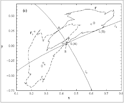
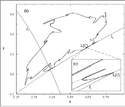
Figure 2: (a) Invariant circle, $\Gamma$, one of its preimages, $\Gamma_{2}^{-1}$, and the critical curves $J_{0}$ and $J_{1}$ ($\tau=1.775$). The image of a “curve” crossing $J_{0}$ (at $A$ and $B$) is tangent to $J_{1}$ (at $L(A)$ and $L(B)$, respectively). (b) “weak chaotic ring” possessing loops ($\tau=1.785$); (c) enlargement showing the loop on the attractor at $L(C)$.

We now define the critical curve $J_{0}$ (termed “curve C” in [16] and often $LC_{-1}$ for Ligne Critique in the recent noninvertible literature [11, 24]) as the locus in phase space where the linearization of the map becomes singular. We call its image $J_{1}$ (“curve D” and $LC$, respectively). The two sets $J_{0}$ and $J_{1}$, as well as additional images and preimages, are known to be a key to understanding the dynamics of a noninvertible map. Consider, for example, Fig. 2a showing an enlargement of the IC, $\Gamma$ for $\tau=1.775$, with three important additions: $J_{0}$, $J_{1}$, and $\Gamma_{2}^{-1}$, one additional first-rank preimage of the invariant circle $\Gamma$. The map $L_{(0.36,1.775)}$ (abbreviated as $L$) has either one or three inverses depending on the phase-plane point in consideration (the term “$Z_{1}-Z_{3}$ map” has been proposed for such maps, [23]). The invariant circle $\Gamma$ has three first-rank preimages: itself, the curve $\Gamma_{2}^{-1}$ shown in the figure, and a third preimage $\Gamma_{3}^{-1}$, further away in phase space (not shown). The geometry of the map can be visualized by first folding the left side of the phase plane along $J_{0}$ and onto the right side. $\Gamma$ and $\Gamma_{2}^{-1}$ should now coincide. Next rotate roughly $90^{\circ}$ so that $J_{0}$ maps to $J_{1}$. The image of $\Gamma$ lands exactly on itself (before the folding), sending $A$ to $L(A)$ and $B$ to $L(B)$ in the process. Note that $L$ maps points that are in the intersection of the two regions bounded by $\Gamma$ and $\Gamma_{2}^{-1}$ to the region bounded by the pieces of $\Gamma$ and $J_{1}$ which connect at $L(A)$ and $L(B)$. That is, some points inside $\Gamma$ are mapped outside $\Gamma$. Similarly, points inside $\Gamma_{2}^{-1}$, but not $\Gamma$ are mapped from outside $\Gamma$ to inside $\Gamma$. Contrast this with the property that interiors of invariant circles for (orientation preserving) invertible maps are invariant.

Note also that $\Gamma$ is tangent to $J_{1}$ at $L(A)$ and $L(B)$. The “folding” along $J_{0}$, typically creates a quadratic tangency along $J_{1}$ at images of curves crossing $J_{0}$, unless the curve crossing $J_{0}$ does so at an angle tangent to the zero eigenvector at that point. This phenomenon has been extensively discussed in [11]. Our explanation here is based on the understanding reached in that paper. As a parameter (in this case $\tau$) is varied, the map $L_{(0.36,\tau)}$ (again abbreviated as $L$), the entire attracting set $\Lambda$, the curves $J_{0}$ and $J_{1}$ as well as the intersection points of $\Lambda$ with $J_{0}$ (e.g. $A$) and with $J_{1}$ (e.g. $L(A)$) vary. In our case, between $\tau$ values for figs. 2a and b, the invariant curve develops a “fjord’ which pushes across $J_{0}$, creating two new intersection points of $\Lambda$ with $J_{0}$, and two new tangencies with $J_{1}$ at the two image points. We call the lower intersection point of the fjord $C$ (see fig. 2b). The points $C$ and $L(C)$ vary with $\tau$ as well. When the tangent of the “curve” in $\Lambda$ at the intersection point $C$ becomes coincident with the null vector of the Jacobian of the map at $C$, the image of $\Lambda$ ($\Lambda$ itself) acquires a cusp touching $J_{1}$ at $L(C)$ [11]. As the parameter value $\tau$ is further varied, the cusp becomes again a quadratic tangency, but $\Lambda$ acquires a loop (figs. 2b and c). Iteration of this “loop” gives rise to an infinity of such loops (called “antennae” in [16]) on $\Lambda$, suggesting chaotic behavior.

Further, Lorenz gives a heuristic justification of a simple criterion for an attractor (not formally defined, but assumed by us to be a compact invariant set with some sort of recurrence) to be a chaotic attractor (an attractor exhibiting sensitivity to initial conditions): the existence of two distinct points on the attracator which map to the same image point (also on the attractor) [16]. In this context, the tracing out of an object with a single orbit suggests recurrence, and existence of a loop implies the existence of two points which map to the same image point. Thus, if this criterion is correct, attractors with loops would necessarily be chaotic attractors.

3.2 Numerical investigation

We set out to examine the transition from smooth IC to chaotic attractor in finer detail in figures 3 to 11. Before we embark on a detailed description, we should state that the real picture is yet more complex, involving similar phenomena on an even finer scale. For example, the same phenomena which cause the destruction of the “large” IC could also destroy the “small” IC’s which we refer to below. Nevertheless, this sequence of figures includes the essential features of the transition: coexistence of a periodic orbit with a nearby IC, destruction of the IC through a global bifurcation, appearance of loops on an unstable manifold, and the reappearance of an attractor, this time chaotic with loops. It might be useful to look ahead to the two-parameter bifurcation diagram in fig. 12 to put the one-parameter cut described in the current section in context.

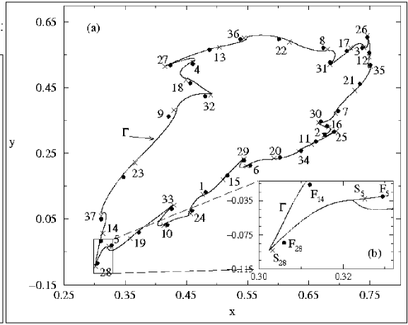
Figure 3: Coexisting attractors for $\tau=1.7765$: the attracting period-$37$ foci ($\bullet$), and the IC. The period-$37$ saddles ($\times$) are also shown, along with both branches of the unstable manifold $S_{5}$. One branch approaches the focus $F_{5}$, while the other branch approaches the IC.

We start from the smooth IC at $\tau=1.775$ (fig. 2a). At $\tau\approx 1.776243$ a period-$37$ saddle and node pair appears in a saddle-node (turning point) bifurcation. The bifurcation occurs off of the IC, and results in the coexistence of two attractors: the stable invariant circle, $\Gamma$, and an attracting period-$37$ sink. Although the sinks have real eigenvalues at the saddle-node bifurcation, the eigenvalues very quickly become complex and they have been labelled in fig. 3b for $\tau=1.7765$ by $F_{i}$ for “focus.” The separatrix between these two coexisting attractors consists of the stable manifolds of the period-$37$ saddles. Global unstable manifolds have been systematically constructed as (37th) forward iterates of local unstable manifolds as for invertible maps. In this case, we have plotted only the two branches emanating from saddle $S_{5}$. The right branch of the global unstable manifold directly approaches $F_{5}$. This is clear in the blowup of fig. 3b. The left branch very quickly approaches the IC $\Gamma$. Successive 37th iterates travel slowly in a clockwise direction around the IC, eventually showing a good approximation to the whole IC. The approach to the IC is somewhat clearer in fig. 3b, where the branch appears to “join” the IC just to the left of $S_{5}$. The unstable manifold then continues almost “on” the IC: past $F_{28}$, $S_{28}$, and $F_{14}$, evolving around the IC, reentering from the right, just below $F_{5}$, before completing the (approximation to the) IC just to the left of $S_{5}$.

Notice also that 18 of the period-$37$ saddle-node pairs are “inside” (those marked by numbers inside $\Gamma$) and the rest “outside” the invariant circle; this is another feature of noninvertible maps [11]). We discuss this again in Sec. 5.

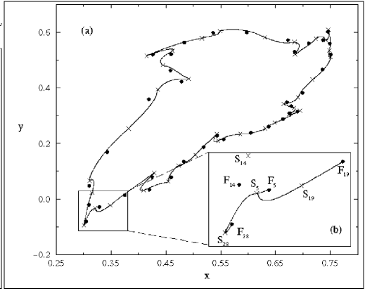
Figure 4: During the “first” manifold crossing ($\tau=1.77688$). a) the period-$37$ saddle and sink solutions have been plotted with one branch of the global unstable manifold (the branch involved in the crossing) which emanates from each of the 37 saddles. b) Both branches of the unstable manifold emanating from the saddle labelled $S_{19}$ have been plotted (but not the branches emanating from $S_{5}$, or any other saddle).

As $\tau$ increases further, the consequences of global bifurcations are observed; these bifurcations involve interactions between the stable and unstable manifolds of the saddle period-$37$ points. The first such global bifurcation is evident in the sequence of figures 3 through 5: the left branch of the unstable manifold of $S_{19}$ misses $S_{5}$ to the left in fig. 3 and approaches the IC (the curve coming into the inset from the right and below $F_{5}$ is practically coincident with this unstable manifold branch); it makes the “saddle connection” with $S_{5}$ in fig. 4; it misses $S_{5}$ to the right in fig. 5 and approaches $F_{5}$.

The global crossing actually “starts” with a heteroclinic tangency (between a branch of a stable manifold of a period-$37$ saddle and and branch of an unstable manifold of another saddle on the same orbit) which destroys the IC at $\tau\approx 1.776878$. This tangency is also called a crisis [25], since as $\tau$ increases toward the tangency parameter value, the IC (approached by the unstable manifold) and its basin boundary (the stable manifold) approach each other, colliding at the tangency parameter value. The attracting set during the crossing appears — as for invertible maps — to be a complicated topological object which at least includes the closure of the unstable manifolds of the period-$37$ saddles. Numerically, most orbits appear to approach the period-$37$ sink (fig. 4). Thirty-seventh iterates of each of the $37$ branches of the unstable manifold plotted in fig. 4a evolve clockwise toward the “next” saddle, suggesting that we are at least close to a heteroclinic crossing of stable and unstable manifolds. Although the stable manifolds of the saddles cannot be realistically computed because of the exponential explosion (“arborescence”) of the number of period-$37$ preimages, the crossing of the stable manifold is evident in the inset (fig. 4b). The left branch of the unstable manifold of $S_{19}$ heads toward saddle $S_{5}$, and although it is not clear from the figure, it begins to alternate back and forth, with folds on the right approaching $F_{5}$, and folds on the left approaching $S_{28}$. The portion approaching $S_{28}$ folds again, with one side heading toward $F_{28}$ (visible) and the other side heading toward $S_{14}$ (only the start is visible). Further iterates (not shown) would result in this one branch of the unstable manifold of $S_{19}$ eventually evolving all the way around the attracting set suggested in fig. 4a, repeatedly visiting every saddle and every node. As with invertible maps, this allows for long chaotic transients, if one could appropriately choose initial conditions on the unstable manifold. Most orbits, however, eventually are attracted to the period-$37$ sink.

We note that a transverse crossing of stable and unstable manifolds in the noninvertible setting does not imply transverse crossings along the rest of the orbit. For this reason, homoclinic or heteroclinic crossings do not necessarily imply the existence of a “horseshoe” or the chaotic transients referred to above. However, Sander [33] shows that the failure of a transverse crossing to provide a horseshoe is a codimension-two phenomenon, so we assume that our transverse crossings in our one-parameter study avoid such a problematic point, and behave as in the invertible case. Thus we expect the parameter value at the tangency initiating this heteroclinic crossing to be an upper bound on $\tau_{CD}$, marking the first appearance of chaotic dynamics. The invariant set with the chaotic dynamics does not appear to be an attractor, however, so the chaos is numerically evident only as transient behavior.

Figure 5: After the first manifold crossing ($\tau=1.778$): the invariant circle as an attractor has disappeared, but a new invariant frequency locked circle has formed as an attracting set. Both branches of the unstable manifold of the two adjacent period-$37$ saddles ($S_{5}$ and $S_{19}$) are plotted. The right branch of the unstable manifold of $S_{5}$ and the left branch of the unstable manifold of $S_{19}$ meet at the attracting focus $F_{5}$.

After the crossing, which ends in a heteroclinic tangency at $\tau\approx 1.776881$, both branches of the unstable manifolds of the period-$37$ saddles approach the period-$37$ sink. The only attractor that remains is the stable period-$37$ sink, shown along with the period-$37$ saddles in fig. 5 for $\tau=1.1778$. The attracting set, however, is a “new” invariant circle, with a period-$37$ locking, formed by connecting the saddles and nodes with the unstable manifolds of the saddles. This invariant circle is seen in the blowup of fig. 5b. It is smooth except at the sinks, where two different branches connnect and the smoothness depends on the eigenvalues [4]. Here the IC is only $C^{0}$ since the sinks are foci, with complex eigenvalues. There are apparently no cusps on the unstable manifolds at this parameter value.

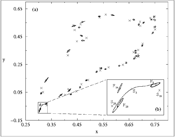
Figure 6: After a secondary Hopf bifurcation of the period-$37$ foci: period-$37$ invariant circles surround unstable foci ($\circ$) at $\tau=1.78$. Both sides of the unstable manifold of the period-$37$ saddles — shown here only for $S_{5}$ — asymptote to the stable period-$37$ invariant circles.

As $\tau$ is increased, a secondary Hopf bifurcation of the period-$37$ foci at $\tau=1.779444$ renders them unstable. This can be seen in fig. 6 for $\tau=1.78$, where the unstable foci, are surrounded by stable period-$37$ invariant circles. It is important (and barely visible in the figure) that the unstable manifold intersects the small invariant circles (and itself!) repeatedly. This is a reminder of the noninvertibility of the map, and our acknowledged abuse of the term “manifold.” See [11] for a discussion of this type of unstable manifold self-intersection.

Figure 7: Locking on the small IC ($\tau=1.7835$). Both branches of the unstable manifold of $S_{5}$ are plotted. Self-intersections are apparent on the right branch. Also shown are period-$37$ saddles ($\times$), period-$37$ repelling foci ($\circ$), and, in (b), period-$259$ sinks ($\bullet$), but not the period-$259$ saddles.

A number of high-period lockings on the period-$37$ invariant circles appear for very narrow ranges of the parameter. For example, at $\tau=1.7835$, a period-$259$ saddle-node pair (formed after a period-7 locking of the period-$37$ invariant circles) is visible (fig. 7); assuming the period-$7$ locking is on the small ICs, these small ICs are now frequency locked circles, composed of the chain of the unstable manifolds of the period-$259$ saddles (not shown). The period-$37$ unstable manifolds asymptotically approach the small ICs. The right branch clearly intersects itself and the IC it approaches (fig. 7b). Most individual orbits eventually approach the attracting period-$259$ sinks.

A second heteroclinic manifold crossing involving the “other” side of the global unstable manifold of the period-$37$ saddle “starts” at $\tau\approx 1.78373$. The bifurcation is apparent in figures 7 through 9: the right branch of the unstable manifold of $S_{5}$ swings around $F_{5}$, and misses $S_{19}$ to the left in fig. 7, approaching the small IC around $F_{5}$; it makes the “saddle connection” with $S_{19}$ in fig. 8; it misses $S_{19}$ to the right in fig. 9, with successive iterates following essentially “on” the attractor with loops.

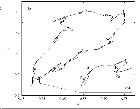
Figure 8: During the “second” manifold crossing ($\tau=1.784$). (a) Unstable manifolds of all $37$ saddles are plotted. (b) Only the two branches of the unstable manifold of $S_{5}$ are plotted; the right branch is the heteroclinic branch. For clarity, neither the period-$296$ saddles nor foci locked on the small ICs are plotted.

As for the earlier manifold crossing, understanding the saddle connection at $\tau=1.784$ requires some explanation. At this parameter value (fig. 8), a period-$8$ resonance on the small invariant circles results in the period-$296$ points apparently being the only attractors. The left branch of the unstable manifold of $S_{5}$ very quickly approaches the small IC surrounding $F_{28}$ and continues counterclockwise around it; it is not a homoclinic loop, although it appears close to being one. The right branch heads for $S_{19}$ after looping clockwise about $3/4$ of the way around $F_{5}$ (including the two high curvature “corners”); the global crossing is apparent since part of the manifold iterates to the left of $S_{19}$ around the IC (we iterated only half way around the IC), and part of the manifold iterates to the right of $S_{19}$ toward the right edge of the inset; this part to the right of $S_{19}$ continues the “long transient” behavior. It is important to notice that although both branches of the unstable manifold of $S_{19}$ are being followed by parts of the right branch of the unstable manifold of $S_{5}$, neither branch of the unstable manifold of $S_{19}$ has been directly plotted in this figure.

Figure 9: (a) Coexistence of period-$407$ attracting orbit with a “weakly chaotic ring” ($\tau=1.785$). Plotted are the period-$37$ saddles ($\times$), period-$37$ repelling foci ($\circ$), period-$407$ attracting nodes ($\bullet$), and the unstable manifolds of the period-$37$ saddles. (b) enlargement with only the two branches of the unstable manifold of $S_{5}$ plotted. (c) Further enlargement of a portion of the saddle global unstable manifold in (b) at $\tau=1.785$ (solid line) with loops; the analogous unstable manifold for the approximate “cusp parameter”: $\tau=1.78428$ (dashed line). Not shown are the period-$245$ saddles and nodes which exist on the small ICs at this cusp parameter value.

The slope of the unstable manifold at the point of intersection with $J_{0}$ continues to change as $\tau$ is increased. At $\tau=\tau_{cusp}\approx 1.78428$ the slope becomes equal to the slope of the eigenvector corresponding to the zero eigenvalue, and cusp points appear on the “manifold” (fig. 9c). Beyond this “cusp parameter” value, the unstable manifold contains loops. Since $\tau_{cusp}$ occurs while the unstable manifold is still intersecting the stable manifold, the picture for $\tau$ just beyond $\tau_{cusp}$, but not beyond the heteroclinic tangency which marks the end of the stable/unstable manifold crossing, is more complicated than might be expected in other families. In our case, the newly developed loops are damped out as they eventually approach the small period-$37$ ICs (possibly with locked solutions on the small ICs). Of course, the loops could follow a long transient before being attracted to the ICs. We do not have a figure corresponding to such a parameter value.

With further increase of $\tau$, we pass the “other end” of the manifold crossing (beyond the final heteroclinic tangency) and an apparently chaotic attractor appears. Thus, this final heteroclinic tangency parameter value appears to be an upper bound on $\tau_{chaos}$, marking the first appearance of a chaotic attractor. At $\tau=1.785$ the resulting attractor is seen in fig. 9 to coexist with a stable period-$407$ (born at a period-$11$ locking on the period-$37$ small invariant circles): the left branch of the unstable manifold of $S_{5}$ approaches the nearby small IC with the period-$407$ locking; the right branch approaches the large amplitude “messy” attractor that self-intersects and exhibits the loops it has inherited from the global unstable manifold. Such an attractor has been called a “weakly chaotic ring” ([11, 24]). Note that Lorenz plotted this weakly chaotic ring attractor by iterating a single orbit starting near the fixed point (fig. 1c); we plotted the same attractor by following a branch of the unstable manifold of the period-$37$ saddle orbit (fig. 9). Tracking the periodic saddles and their manifolds also allowed us to see the coexisting small IC with the period-$407$ attractor which was not apparent in fig. 1c.

The small amplitude invariant circles now begin to shrink, disappearing at $\tau\approx 1.78626168$ in a second secondary Hopf bifurcation; the period-$37$ foci from return from sources to sinks; these continue to coexist with the large attractor that has become very “messy” with many more points of self-intersection (fig. 10b for $\tau=1.7866$). The stable period-$37$ foci approach the period-$37$ saddles in anticipation of the following period-$37$ saddle-node bifurcation, which happens at $\tau\approx 1.7866262$.

Figure 10: Coexistence of period-$37$ attracting orbit with a “weakly chaotic ring” ($\tau=1.7866$). (a) Plotted are the period-$37$ saddles ($\times$), period-$37$ attracting nodes ($\bullet$), and the unstable manifolds of the period-$37$ saddles. (b) Enlargement with only the two branches of the unstable manifold of $S_{5}$ plotted. The left branch immediately approaches the period-$37$ stable orbit ($F_{28}$); the right branch approaches the “big” attractor: it iterates off the figure to the right, follows counterclockwise around the attractor seen in (a), and returns in the bottom of (b), coming in just to the right of $F_{28}$ and $S_{5}$; its loops are larger than in fig. 9b.

Figure 11: Only the chaotic attractor remains ($\tau=1.788$). It was approximated by computing a single orbit. The period-$37$ fixed points have disappeared in a saddle-node bifurcation.

Finally, at $\tau=1.788$ the saddle-node bifurcation of the period-$37$ solutions has occurred, and the pair has disappeared. Note that (as with invertible maps) the pairings have switched. For example, $S_{5}$ disappears with $F_{28}$, while $F_{5}$ disappears with $S_{19}$. Only the large chaotic attractor is left, seen in fig. 11.

Recap. The transition from smooth IC attractor ($\tau=1.75$, figs. 1b, 2a) to noninvertible “messy” chaotic attractor ($\tau=1.788$, fig. 11) is not a result of a smooth change of a smooth, large amplitude invariant circle which develops cusps at a critical parameter value. Instead, the transition occurs via a sequence of bifurcations, notably involving the interaction of the IC with nearby periodic orbits and the unstable manifolds of the saddles. Specifically, the IC as an attractor is destroyed in a global manifold crossing that leaves an attracting periodic orbit as the only attractor. The global unstable manifolds of the saddle period-$37$ points are the invariant objects that first develop cusps (at $\tau_{cusp}\approx 1.78428$, fig. 9c) and later loops (beyond $\tau_{cusp}$). When the cusps and loops first appear, they “damp out” as they approach the attracting periodic orbit (or small IC). When the large amplitude attractor reappears at after the second global manifold crossing, it is approached by the branch of the unstable manifold which now has loops. These loops are inherited by the large amplitude attractor which is now apparently chaotic.

4 The larger picture.

Figure 12: (a) The start of a two-parameter bifurcation diagram for the map $L_{(a,\tau)}$, containing the fixed-point Hopf bifurcation curve HB₁, and three pairs of saddle-node curves emanating from HB₁ corresponding to period-$5$, period-$6$, and period-$37$ resonance horns. The $\times$’s are labelled by the phase portraits in fig. 1. (b) An enlargement of the period-$37$ resonance horn where it is traversed in our one-parameter cut. The two period-$37$ saddle-node curves (SN₃₇) mark the upper and lower boundaries of the resonance horn. Two equal eigenvalue curves and a secondary Hopf curve (HB₃₇) subdivide the horn. The parameter values marked with $\times$’s are labelled by our corresponding figure number(s).

While a rich dynamical picture occurs along our one-parameter family with respect to $\tau$, it is clear that it only constitutes a part of a larger, actually two-parameter scenario. This is consistent with existing two-parameter descriptions of Hopf bifurcations for invertible maps [3, 4, 6, 26, 27, 28]. The primary features in the invertible case are resonance horns — inside which the corresponding maps have a periodic orbit of a certain period — emanating from the primary Hopf bifurcation curve. Since the fixed point at a Hopf bifurcation has eigenvalues on the unit circle, the IC close to its birth lies far away in phase space from $J_{0}$, where the map has a zero eigenvalue. Thus, we expect the two-parameter bifurcation diagram for the noninvertible Hopf bifurcation to strongly resemble the analogous bifurcation diagram for the invertible case — at least near the Hopf bifurcation curve.

We have embedded our one-parameter family ($a=0.36$ in eq. (3)) in the two-parameter family $L_{(a,\tau)}$. Fig. 12a shows part of the “big picture” in the $\tau$-$a$ plane: the period-one Hopf bifurcation curve together with period-$37$, period-$5$, and period-$6$ resonance horns emanating from it. The bifurcation points we encountered along the one-parameter cut “continue” to bifurcation curves in the two-parameter setting. The curves displayed in this figure are only a tiny sampling of the dozens of bifurcation curves we have computed, which are, in turn, only a tiny sampling of the bifurcation curves that can be computed for this family. (In particular, there are saddle-node curves in addition to those emanating from the primary Hopf bifurcation curve. See [22, 29] for descriptions of such intraresonance horn features for invertible maps.)

As we move higher up in the horns — above the “IC tangent to $J_{0}$” curve in fig. 12a — the circle grows and starts to interact with $J_{0}$ and thus becomes “truly” noninvertible. It is above this curve where the corresponding maps can exhibit noninvertible behavior, such as mapping some of the interior of an IC to its exterior and vice versa (recall fig. 2a). More “interesting” behavior, such as coexisting attractors or the breakup of the IC, is suggested when the resonance horns start to overlap. In our one-parameter cut this overlap happens at least by the first period-$37$ sadde-node bifurcation at $\tau\approx 1.776243$, although the three horns we have displayed do not overlap until higher $\tau$ values.

The enlargement in fig. 12b shows three of the multitude of bifurcation curves which subdivide the period-$37$ horn into “inequivalent” regions: two “equal eigenvalue” curves (just inside the horn), marking the transition between real and complex eigenvalues for a period-$37$ orbit, and a secondary Hopf curve (HB₃₇), marking the birth of the “period-$37$ small ICs.” Somewhat unsatisfying in fig. 12b is the fact that none of the displayed bifurcation curves is unique to noninvertible maps. We remark that we did compute an “eigenvalue zero” curve (for the existence of a period-$37$ point with an eigenvalue of zero), but we did not display it in fig. 12b because it had no direct bearing on the bifurcation sequence we described (but see such a curve in a period-$6$ horn in fig. 13). However, this curve certainly has an indirect bearing on the bifurcations, because it is related to the crossing of $J_{0}$ by the attracting set (which includes any ICs, periodic orbits, and their unstable manifolds). If the attracting set never interacted with $J_{0}$, the bifurcations could be produced with invertible maps.

Other bifurcation curves, which our current computational tools did not handle easily, would separate the other $\times$’s in fig. 12b from each other. For example, the $\times$ labelled 4 is in a thin heteroclinic region; heteroclinic tangency curves separate it from 3 below and 5 above. Similarly, the $\times$’s labelled 8 and 9c are in a thin heteroclinic region, separating them from 7 below and 9 above. A “cusp curve” (unique to noninvertible resonance horns) runs through 9c. The $\times$ labelled 7 is in a thin “period-$259$ secondary resonance horn,” which emanates from the secondary Hopf curve HB₃₇ and corresponds to a locking on the small period-$37$ ICs.

A more complete knowledge of the internal structure of the “noninvertible” resonance horns in the two-parameter setting is clearly the key to extending our current understanding of the transition from a smooth invariant circle to a chaotic attractor.

5 Discussion

5.1 Typical one-parameter cuts

A natural question which arises following the detailed numerical investigation of Sec. 3 is how “typical” are the features of that specific one-parameter family. We take the liberty in the next few paragraphs of using the intuition we have gained via our numerical explorations, including the partial two-parameter bifurcation diagram of the previous section, to provide at least a partial answer to this question. Even though somewhat speculative, we feel that these observations are useful for placing the one-parameter cut in a broader context.

A key observation accompanying our understanding of the IC breakup is that an IC with a cusp and an irrational rotation number would have the cusp iterate forward to a dense set of image points, which would also be cusps. Even if such an object is topologically possible, it appears to us to be highly unlikely. Because of this, we expect the invariant circle to break up before it reaches a parameter value where it develops a cusp. Thus, the IC must interact with some other object in the attracting set. In our experience, the other object in this “pre-cusp” breakup is a nearby periodic orbit and its accompanying stable and unstable manifolds. The related manifold crossings appear to be the “natural” way to first destroy an existing IC and to later reconstitute “itself” as a chaotic attractor.

This observation is consistent with the sequence of transitions we described in Sec. 3. Extending this one-parameter transition interval to the two-parameter setting, we imagine a transition band, roughly parallel to the ‘IC tangent to $J_{0}$’ curve, and passing between parameter values labelled ‘1b’ and ‘1d’ in fig.12a. Below the lower boundary of the transition band a smooth invariant circle exists (possibly locked, possibly coexisting with periodic orbit(s)). Above the upper boundary of the transition band, the corresponding maps are chaotic. Loosely, the transition band is a “thick version” of the “cusp curve” suggested by Lorenz.

Further supporting this transition band scenario is the prominent “opening” of the resonance horns in fig. 12a. This would be even more prominent if more resonance horns were plotted: most of the resonance horns appear to open up and overlap near the top of the upper boundary of the transition band. This is suggestive of, or at least consistent with, chaos.

The existence of the transition band also suggests why the period-$37$ orbit might have been the specific orbit that was involved in our one-parameter scenario: that was the horn which was passed through as the transition to chaos band was crossed. Vertical parameter cuts for values of $a$ other than $a=0.36$ could pass through a different periodic horn during this narrow transitional parameter interval. We note that Lorenz specifically chose $a=0.36$ because it appeared to “avoid periodic windows.” In the two-parameter context, this can be interpreted as avoiding low-period resonance horns. Thus, we might expect a “typical” one-parameter cut to often interact with a periodic orbit of a period less than $37$.

Alternative viable bifurcation sequences are suggested by the blowup of the period-$37$ horn in fig. 12b. For example, moving the cut to the left of $a=0.3599$ could avoid the secondary Hopf bifurcation curve HB₃₇, and thus avoid the small invariant circles that appeared in the $a=0.36$ cut. Other differences in varying $a$ would be more obvious if we were able to compute the region(s) of the period-$37$ horn corresponding to the global bifurcations, and curves corresponding to the development of cusps. (We expect to be able to do this in the future.) We know the $\times$ labelled ‘$9c$’ in fig. 12b is both on a cusp curve (in the parameter space) and in a heteroclinic region. Moving the vertical cut either left or right would probably prevent these two from coinciding. That is, the fact that the cusp parameter value occured during the manifold crossing in the $a=0.36$ cut is probably not typical of most one-parameter cuts. If the cusp parameter value occured first (with respect to $\tau$), then the phase portrait for the first appearance of loops would be simpler: the loops would simply approach the small attracting ICs. (If we encountered the cusp parameter outside the secondary Hopf curve, it would be still simpler: the loops would damp out at the attracting period-$37$ nodes. See fig. 15 for comparison.) On the other hand, if the cusp parameter value occured after the heteroclinic region had been crossed, we claim (with no proof) that there must be another periodic orbit interacting with the IC as well. Perhaps its unstable manifold will be the one to develop a cusp and later undergo a global manifold crossing to reconstitute the chaotic attractor with loops.

5.2 Related noninvertible features

The relatively high period of the locking encountered along the one-parameter cut above makes the elucidation of the phase and parameter space structures cumbersome. To illustrate some of these phenomena more succinctly we perform computations in the neighborhood of a simpler (period-$6$) resonance horn.

Figure 13: Period-$6$ resonance horn and related bifurcation curves.

Fig. 13 is a blow-up of this period-$6$ resonance horn, with two additional types of bifurcation curves plotted inside: (a) two global bifurcation curves (approximating a thin heteroclinic manifold crossing region associated with the stable and unstable manifolds of the period-$6$ saddle points) and (b) the curve on which the periodic points acquire an eigenvalue zero (i.e. one periodic point lies on $J_{0}$ and one on $J_{1}$) [13, 12]. This latter curve provides an indication of the interaction of the dynamics with noninvertibility. An additional curve (‘IC tangent to $J_{0}$’), extending beyond the resonance horn, is plotted. This is the locus, in parameter space, where the invariant circle starts interacting with noninvertibility, by first touching the critical curve $J_{0}$. Note that the ‘eigenvalue zero’ curve is tangent to the ‘IC tangent to $J_{0}$’ curve.

Figure 14: Inside the horn: Period-$6$ saddle-node pairs inside and outside the invariant circle ($a=0.465$, $\tau=1.472$); the hatched region inside $\Gamma$ is mapped to the grey region outside.

In fig. 14, we show a phase portrait for a parameter value inside the period-$6$ horn and above the ‘IC tangent to $J_{0}$’ curve ( $(a,\tau)=(0.465,1.472)$ ). The invariant circle crosses $J_{0}$ transversely at two points $A$ and $B$; it is easy to see that it will then become quadratically tangent to $J_{1}$ at the image points $L(A)$ and $L(B)$ (see [11, 24]). Also illustrated in the figure is the relative location of the attracting invariant circle and one more of its three first-rank preimages. Clearly, one of the period-$6$ saddle-node pairs is located inside the attracting invariant circle while the remaining five are located outside. (Note that iterates of points to the left of $J_{0}$ switch sides of the IC; thus, there must be an even number of periodic points to the left of $J_{0}$.) We have also illustrated the portion of the interior of the invariant circle that is mapped “outside” after one iteration of the map, as well as the portion of phase space outside the invariant circle that gets mapped inside.

Our next observation is for another parameter value inside the period-$6$ horn: $(a,\tau)=(0.4838,1.409)$. In fig. 15 we have an example of an unstable manifold of a period-$6$ saddle with a cusp which damps out at the period-$6$ attracting orbit. Recall that in our one-parameter cut, the cusp on the period-$37$ unstable manifold developed in the middle of a heteroclinic crossing. Iterates of the cusp could therefore follow a long transient before eventually being damped out as it approached a period-$37$ sink. Fig. 15 is a simpler version of the damping out of cusps on an unstable manifold in the approach to a sink.

Figure 15: Simple damping out of a cusp at an attracting period-$6$ node ($(a,\tau)=(0.4838,1.409)$ ). (b) The upper right cusp maps (under $L^{6}_{(0.4838,1.409)}$) to what looks like the end of a line segment emanating from $N_{1}$. The whole unstable “manifold” has effectively collapsed onto this line. Successive (sixth) iterates of the cusp approach $N_{1}$ along the line.

Finally, we have made an attempt to illustrate the complexity of the basins of attraction of the coexisting attractors: the stable period-$6$ points and the stable invariant circle. While for the purposes of this paper we will not dwell on the details of this complicated structure (for a discussion of the basic building blocks of such a picture see again [11] as well as [2, 9, 10, 13, 12, 5]), we emphasize a few key elements:

• the basins of attraction are not simply connected;

• the stable “manifolds” consist of a large number (possibly, even an infinity) of branches (resulting from the multiple backward in time trajectories). Only the computed “immediate” local manifold of the period-$6$ saddles is shown in fig. 16; the images and preimages of them form the boundaries of the grey disconnected “islands” that belong to the basin of attraction of the period-$6$ foci.

• notice that the stable set intersects $J_{0}$. The images and preimages of the intersection points have been called “points of alternance” [18] on parts of the stable manifolds: these are points (on $J_{0}$ and its preimages) where two preimages of a branch of the stable set come together; the “direction of relative movement” of nearby points switches at such points of alternance.

Figure 16: Basin of attraction of the period-$6$ foci marked by filled circles (grey region) and of the coexisting invariant circle (the white complement) at $(a,\tau)=(0.45,1.563)$. The computed “immediate” stable manifolds of the period-$6$ saddles (marked by crosses) are also plotted.

5.3 Computational issues

As a final comment on the current state of our work on noninvertible systems, we note that computational tools for the accurate approximation and visualization of objects such as stable and unstable manifolds are crucial in both understanding what is possible and in analyzing specific examples. The possibility of multiple inverses can cause an exponential explosion in the number of distinct segments of an invariant curve or of stable manifolds of periodic points. The same is true for the critical set: all the images and preimages of the critical curve $J_{0}$. In three dimensions the computational issues are even further complicated: the $J_{0}$ curve becomes a surface, and its iterates and preiterates must be constructed. Standard one-dimensional continuation tools have to be extended (to simplicial continuation, or through software like PISCES [34]) to effectively compute, triangulate and visualize these surfaces and their intersections. Constructing scientific computing, database management and visualization tools for these objects in two and three dimensions is an important task, and to our knowledge, an open area of research. Development of these tools would facilitate the analysis of many physical systems that are inherently noninvertible: discrete-time adaptation, control and decision problems, ranging from Model Reference Adaptive Control systems to signal processing applications -in addition to more traditional noninvertible models arising in population dynamics and economics. These tools will also be applicable in the case of multiple forward trajectory systems (such as those arising in implicit integrators, or in model predictive control), as well as, more generally, in relations [17].

6 Conclusions

The breakup of invariant circles in invertible maps of the plane possess a relatively well-studied dynamic phenomenology; homoclinic tangles of the invariant manifolds of nearby periodic saddle points, which arise from lockings on or off the invariant circle, play an important role in the two-parameter picture. Invariant circles for noninvertible maps of the plane possess, in some sense, an even “richer” phenomenology. Initially, close to the Hopf bifurcation giving rise to them, they are locally invertible, and the Arnold horn scenario holds. Large amplitude noninvertible invariant circles, however, may interact with the critical curves of the map. This can (and does) lead to new transitions and bifurcations. We demonstrated that the one-parameter transition discovered in [16] actually constitutes a part of the interior structure of the Arnold horns in the noninvertible two-parameter setting; we placed it in the appropriate context by pointing out the role of nearby periodic points and their stable and unstable manifolds. The picture we have presented here is far from complete, however we hope that our work is a step toward a more complete understanding of the transition from smooth invariant circle to chaotic attractor in the presence of noninvertibility.

Acknowledgments. Besides being motivated by the original work of Professor E. Lorenz, we acknowledge extensive discussions with him when this paper was first being developed in the early and mid 1990’s. He declined, however, being a co-author of the paper, something that we believe he deserved, and we note this here. We also acknowledge discussions with Prof. R. Rico-Martinez of the Instituto Tecnologico de Celaya (Mexico) and Prof. C. Mira of the Complexe Scientifique de Rangueil, Toulouse, France. We also acknowledge the support of the National Science Foundation (IGK and BBP: Grant No. DMS-9973926), and the Swiss Office of Energy (CEF). Any opinions, findings, and conclusions or recommendations expressed in this paper are those of the authors and do not necessarily reflect the views of the funding agencies.

References

- [1] Abraham R H, Gardini L and Mira C, “Chaos in Discrete Dynamical Systems,” Springer-Verlag (TELOS) New York (1997).
- [2] Adomaitis R A and Kevrekidis I G, “Noninvertibility and the structure of basins of attraction in a model adaptive control system,” J. Non Linear Sci., 1, 95-105, (1991).
- [3] Arnold V I, Geometric Methods in the Theory of Ordinary Differential Equations, Springer-Verlag, New York, (1983).
- [4] Aronson D G, Chory M A, Hall G R, and McGehee R P, “Bifurcations from an invariant circle for two-parameter families of maps of the plane: A computer assisted study,” Commun. Math. Phys., 83, 303-354, (1982).
- [5] Billings L and Curry J H, “On noninvertible maps of the plane: Eruptions,” Chaos 6 108, (1996).
- [6] Chenciner A, “Bifurcation de points fixes elliptiques. II. Orbites périodiques et ensembles de Cantor invariants,” Inventiones Mathematicae, 80, 81-106, (1985).
- [7] Collet P, and Eckmann J-P , “Iterated maps of the interval as dynamical systems,” Birkhäuser, (1980).
- [8] Feigenbaum M, “Quantitative universality for a class of nonlinear transformations,” J. Stat. Phys., 19(1), 25-52, (1978).
- [9] Frouzakis C E, Adomaitis R A, and Kevrekidis I G, “On the dynamics and global stability characteristics of an adaptive control system,” Comp. Chem. Eng. 20 Suppl. B pp.1029-1034, (1996).
- [10] Frouzakis C E, Adomaitis R A, Kevrekidis I G, Golden M P, Ydstie B E, “The structure of basin boundaries in a simple adaptive control system,” in Chaotic Dynamics: Theory and Practice, T. Bountis, ed., 195-210, Plenum Press, NY, (1992).
- [11] Frouzakis C E, Gardini L, Kevrekidis I G, Millerioux G and Mira C, “On some properties of invariant sets of two-dimensional noninvertible maps,” Int. J. Bif. Chaos, 7(6), (1997).
- [12] Gicquel N, Anderson J S, Kevrekidis I G, “Noninvertibility and resonance in discrete-time neural networks for time-series processing,” Phys. Lett. A 238(1) (1998).
- [13] Gicquel N, Frouzakis C E, Kevrekidis I G, “Invariant circles of plane endomorphisms: a computer-assisted study,” CESA’96, Computational Engineering in Systems Applications, Lille, July 9-12, (1996).
- [14] Gumowski I and Mira C, “Recurrences and discrete dynamic systems,” Springer Verlag, Singapore, (1980).
- [15] Lorenz E N, “Deterministic nonperiodic flow,” J. Atmos. Sci., 20,130, (1963).
- [16] Lorenz E N, “Computational Chaos - A prelude to computational instability,” Phys. D, 35, 299-317, (1989).
- [17] McGehee R P, “Attractors for closed relations on compact Hausdorff spaces,” Indiana U. Math. J., 41(4), 1165-1209, (1992).
- [18] Mira C, “Chaotic dynamics,” World Scientific, Singapore, (1987).
- [19] McGehee R P and Nien C-H, “The images of the singular sets for two-dimensional quadratic maps,” preprint.
- [20] McGehee R P and Sander E, “A new proof of the stable manifold theorem,” Z angew Math Phys 47, 497-513, (1996).
- [21] Nien C-H “Analyticity of the center-unstable manifold,” preprint, U. of Minnesota, (1996).
- [22] McGehee R P and Peckham B B, “Arnold flames and resonance surface folds,” Geometry Center Research Report GCG84 and International Journal of Bifurcations and Chaos 6, No. 2 (1996) 315-336.
- [23] Mira C, Fournier-Prunaret D, Gardini L, Kawakami H, Cathala J-C, “Basin bifurcations of two-dimensional nonvinvertible maps. Fractalization of basins,” Int. J. of Bif. and Chaos, 4(2), 343-381, (1994).
- [24] Mira C, Gardini L, Barugola A, and Cathala J-C , “Chaotic Dynamics in Two-Dimensional Noninvertible Maps,” World Scientific, Singapore, (1996).
- [25] Ott E, “Chaos in Dynamical Systems,” Cambridge University Press, New York, 1993.
- [26] Peckham B B, “The closing of resonance horns for periodically forced oscillators,” Thesis, University of Minnesota, 1988.
- [27] Peckham, B B,“The Necessity of the Hopf Bifurcation for Periodically Forced oscillators with closed resonance regions,” Nonlinearity 3 261-280, 1990.
- [28] Peckham B B, Frouzakis C, and Kevrekidis I G, “Bananas and Banana Splits: A parametric degeneracy in the Hopf bifurcation for maps,” SIAM J. Math. Anal. 26, No. 1, 190-217, 1995.
- [29] Peckham B B and Kevrekidis I G, “Lighting Arnold flames: resonance in doubly forced periodic oscillators,” Nonlinearity 15, 405-428, 2002.
- [30] Robinson C, “Dynamical Systems: Stability, Symbolic Dynamics, and Chaos,” CRC Press Inc., Boca Raton, Florida, 1995.
- [31] Rico-Martinez R, Adomaitis R A, and Kevrekidis I G, “Noninvertibility in neural networks, ” Computers and Chemical Engineering 24, 2417-2433(2000).
- [32] Sander E, “Hyperbolic sets for noninvertible maps and relations,” Disc. Cont. Dyn. Systems, 5(2):339-358, (1999).
- [33] Sander E, “Homoclinic tangles for noninvertible maps,” Nonlinear Analysis 41 259-276 (2000).
- [34] Wicklin F J, “PISCES: a platform for implicit surfaces and curves and the exploration of singularities,” manual available on-line at the URL http://www.geom.umn.edu/locate/pisces, (1995).