Hexagonal circle patterns with constant intersection angles and discrete Painlevé and Riccati equations

Abstract

Hexagonal circle patterns with constant intersection angles mimicking holomorphic maps $z^{c}$ and ${\rm log}(z)$ are studied. It is shown that the corresponding circle patterns are immersed and described by special separatrix solutions of discrete Painlevé and Riccati equations. The general solution of the Riccati equation is expressed in terms of the hypergeometric function. Global properties of these solutions, as well as of the discrete $z^{c}$ and ${\rm log}(z)$, are established.

1 Introduction. Hexagonal circle patterns and $z^{c}$

The theory of circle patterns is a rich fascinating area having its origin in the classical theory of circle packings. Its fast development in recent years is caused by the mutual influence and interplay of ideas and concepts from discrete geometry, complex analysis and the theory of integrable systems.

The progress in this area was initiated by Thurston’s idea [24],[17] of approximating the Riemann mapping by circle packings. Classical circle packings consisting of disjoint open disks were later generalized to circle patterns where the disks may overlap (see for example [15]). Different underlying combinatorics were considered. Circle patterns with the combinatorics of the square grid were introduced in [22]; hexagonal circle patterns were studied in [8] and [9].

The striking analogy between circle patterns and the classical analytic function theory is underlined by such facts as the uniformization theorem concerning circle packing realizations of cell complexes with prescribed combinatorics [6], a discrete maximum principle and Schwarz’s lemma [20], rigidity properties [17],[15] and a discrete Dirichlet principle [22].

The convergence of discrete conformal maps represented by circle packings was proven in [21]. For prescribed regular combinatorics this result was refined. $C^{\infty}$-convergence for hexagonal packings is shown in [14]. The uniform convergence for circle patterns with the combinatorics of the square grid and orthogonal neighbouring circles was established in [22].

The approximation issue naturally leads to the question about analogs to standard holomorphic functions. Computer experiments give evidence for their existence [13],[16], however not very much is known. For circle packings with hexagonal combinatorics the only explicitly described examples are Doyle spirals [12],[5], which are discrete analogs of exponential maps, and conformally symmetric packings, which are analogs of a quotient of Airy functions [7]. For patterns with overlapping circles more explicit examples are known: discrete versions of ${\rm exp}(z)$, ${\rm erf}(z)$ [22], $z^{c}$, ${\rm log}(z)$ [2] are constructed for patterns with underlying combinatorics of the square grid; $z^{c}$, ${\rm log}(z)$ are also described for hexagonal patterns [8], [9].

It turned out that an effective approach to the description of circle patterns is given by the theory of integrable systems (see [10],[8],[9]). For example, Schramm’s circle patterns are governed by a difference equation which is the stationary Hirota equation (see [22]). This approach proved to be especially useful for the construction of discrete $z^{c}$ and ${\rm log}(z)$ in [2],[8],[9],[10] with the aid of some isomonodromy problem. Another connection with the theory of discrete integrable equations was revealed in [2],[3],[4]: embedded circle patterns are described by special solutions of discrete Painlevé II and discrete Riccati equations.

In this paper we carry the results of [2] for square grid combinatorics over to hexagonal circle patterns with constant intersection angles introduced in [9].

Hexagonal combinatorics are obtained on a sub-lattice of ${\mathbb{Z}}^{3}$ as follows: consider the subset

$$H=\{(k,l,m)\in{\mathbb{Z}}^{3}:\ |k+l+m|\leq 1\}$$

and join by edges those vertices of $H$ whose $(k,l,m)$-labels differ by 1 only in one component. The obtained quadrilateral lattice $QL$ has two types of vertices: for $k+l+m=0$ the corresponding vertices have 6 adjacent edges, while the vertices with $k+l+m=\pm 1$ have only 3. Suppose that the vertices with 6 neighbors correspond to centers of circles in the complex plane $\mathbb{C}$ and the vertices with 3 neighbors correspond to intersection points of circles with the centers in neighboring vertices. Thus we obtain a circle pattern with hexagonal combinatorics.

Circle patterns where the intersection angles are constant for each of 3 types of (quadrilateral) faces (see Fig.1) were introduced in [9]. A special case of such circle patterns mimicking holomorphic map $z^{c}$ and ${\rm log}(z)$ is given by the restriction to an $H$-sublattice of a special isomonodromic solution of some integrable system on the lattice ${\mathbb{Z}}^{3}$. Equations for the field variable $z:{{\mathbb{Z}}^{3}}\to{\mathbb{C}}$ of this system are:

$$q(z_{k,l,m},z_{k,l+1,m},z_{k-1,l+1,m},z_{k-1,l,m})=e^{-2i\alpha_{1}},$$

$$q(z_{k,l,m},z_{k,l,m-1},z_{k,l+1,m-1},z_{k,l+1,m})=e^{-2i\alpha_{2}},$$ (1)

$$q(z_{k,l,m},z_{k+1,l,m},z_{k+1,l,m-1},z_{k,l,m-1})=e^{-2i\alpha_{3}},$$

where $\alpha_{i}>0$ satisfy $\alpha_{1}+\alpha_{2}+\alpha_{3}=\pi$ and

$$q(z_{1},z_{2},z_{3},z_{4})=\frac{(z_{1}-z_{2})(z_{3}-z_{4})}{(z_{2}-z_{3})(z_{4}-z_{1})}$$

is the cross-ratio of elementary quadrilaterals of the image of ${{\mathbb{Z}}^{3}}$. Equations (1) mean that the cross-ratios of images of faces of elementary cubes are constant for each type of faces, while the restriction $\alpha_{1}+\alpha_{2}+\alpha_{3}=\pi$ ensures their compatibility.

The isomonodromic problem for this system (see section 2 for the details, where we present the necessary results from [9] ) specifies the non-autonomous constraint

$$cz_{k,l,m}=2k\frac{(z_{k+1,l,m}-z_{k,l,m})(z_{k,l,m}-z_{k-1,l,m})}{z_{k+1,l,m}-z_{k-1,l,m}}+$$

$$\qquad\qquad 2l\frac{(z_{k,l+1,m}-z_{k,l,m})(z_{k,l,m}-z_{k,l-1,m})}{z_{k,l+1,m}-z_{k,l-1,m}}+$$ (2)

$$\qquad\qquad 2m\frac{(z_{k,l,m+1}-z_{k,l,m})(z_{k,l,m}-z_{k,l,m-1})}{z_{k,l,m+1}-z_{k,l,m-1}},$$

which is compatible with (1) (this constraint in the two-dimensional case with $c=1$ first appeared in [18]). In particular, a solution to (1),(2) in the subset

$$Q=\{(k,l,m)\in{{\mathbb{Z}}^{3}}|\ k\geq 0,\ l\geq 0,\ m\leq 0\}$$ (3)

is uniquely determined by its values

$$z_{1,0,0},\ z_{0,1,0},\ z_{0,0,-1}.$$

Indeed, the constraint (2) gives $z_{0,0,0}=0$ and defines $z$ along the coordinate axis $(n,0,0)$, $(0,n,0)$, $(0,0,-n)$. Then all other $z_{k,l,m}$ with $(k,l,m)\in Q$ are calculated through the cross-ratios (1).

Proposition 1

[9] The solution $z:Q\to{\mathbb{C}}$ of the system (1),(2) with the initial data

$$z_{1,0,0}=1,\ z_{0,1,0}=e^{i\phi},\ z_{0,0,-1}=e^{i\psi}$$ (4)

determines a circle pattern. For all $(k,l,m)\in Q$ with even $k+l+m$ the points $z_{k\pm 1,l,m}$, $z_{k,l\pm 1,m}$, $z_{k,l,m\pm 1}$ lie on a circle with the center $z_{k,l,m}$, i.e. all elementary quadrilaterals of the $Q$-image are of kite form.

Moreover, equations (1) (see lemma 1 in section 3) ensure that for the points $z_{k,l,m}$ with $k+l+m=\pm 1$ where 3 circles meet intersection angles are $\alpha_{i}$ or $\pi-\alpha_{i}$, $i=1,2,3$ (see Fig.1 where the isotropic case $\alpha_{i}=\pi/3$ of regular and $Z^{3/2}$-pattern are shown).

According to proposition 1, the discrete map $z_{k,l,m}$, restricted on $H$, defines a circle pattern with circle centers $z_{k,l,m}$ for $k+l+m=0$, each circle intersecting 6 neighboring circles. At each intersection points three circles meet.

However, for most initial data $\phi,\psi\in{\mathbb{R}}$, the behavior of the obtained circle pattern is quite irregular: inner parts of different elementary quadrilaterals intersect and circles overlap. Define $Q_{H}=Q\cap H$.

Definition 1

[9] The hexagonal circle pattern $Z^{c}$, $0<c<2$ with intersection angles $\alpha_{1},\alpha_{2},\alpha_{3}$, $\alpha_{i}>0$, $\alpha_{1}+\alpha_{2}+\alpha_{3}=\pi$ is the solution $z:Q\to{\mathbb{C}}$ of (1) subject to (2) and with the initial data

$$z_{1,0,0}=1,\ z_{0,1,0}=e^{ic(\alpha_{2}+\alpha_{3})},\ z_{0,0,-1}=e^{ic\alpha_{3}}$$ (5)

restricted to $Q_{H}$.

Figure 1: Hexagonal circle patterns as a discrete conformal map.

Definition 2

A discrete map $z:Q_{H}\to{\bf C}$ is called an immersion, if inner parts of adjacent elementary quadrilaterals are disjoint.

The main result of this paper is the following theorem.

Theorem 1

The hexagonal $Z^{c}$ with constant positive intersection angles and $0<c<2$ is an immersion.

The proof of this property follows from an analysis of the geometrical properties of the corresponding circle patterns and analytical properties of the corresponding discrete Painlevé and Riccati equations.

The crucial step is to consider equations for the radii of the studied circle patterns in the whole $Q$-sublattice with even $k+l+m$. In section 3, these equations are derived and the geometrical property of immersedness is reformulated as the positivity of the solution to these equations. Using discrete Painlevé and Riccati equations in section 4 we present the proof of the existence of a positive solution and thus complete the proof of immersedness. In section 6, we discuss possible generalizations and corollaries of the obtained results. In particular, circle patterns $Z^{2}$ and $\rm Log$ with both square grid and hexagonal combinatorics are considered. It is also proved that they are immersions.

2 Discrete $Z^{c}$ via a monodromy problem

Equations (1) have the Lax representation [9]:

$$\Phi_{k+1,l,m}(\mu)=L^{(1)}(e,\mu)\Phi_{k,l,m}(\mu),$$

$$\Phi_{k,l+1,m}(\mu)=L^{(2)}(e,\mu)\Phi_{k,l,m}(\mu),$$ (6)

$$\Phi_{k,l,m+1}(\mu)=L^{(3)}(e,\mu)\Phi_{k,l,m}(\mu),$$

where $\mu$ is the spectral parameter and $\Phi(\mu):{{\mathbb{Z}}^{3}}\to{\rm GL}(2,{\mathbb{C}})$ is the wave function. The matrices $L^{(n)}$ are defined on the edges $e=(p_{out},p_{in})$ of ${{\mathbb{Z}}^{3}}$ connecting two neighboring vertices and oriented in the direction of increasing $k+l+m$:

$$L^{(n)}(e,\mu)=\left(\begin{array}[]{cc}1&z_{in}-z_{out}\\ \mu\frac{\Delta_{n}}{z_{in}-z_{out}}&1\end{array}\right),$$ (7)

with parameters $\Delta_{n}$ fixed for each type of edges. The zero-curvature condition on the faces of elementary cubes of ${{\mathbb{Z}}^{3}}$ is equivalent to equations (1) with $\Delta_{n}=e^{i\delta_{n}}$ for properly chosen $\delta_{n}$. Indeed, each elementary quadrilateral of ${{\mathbb{Z}}^{3}}$ has two consecutive positively oriented pairs of edges $e_{1},e_{2}$ and $e_{3},e_{4}$. Then the compatibility condition

$$L^{(n_{1})}(e_{2})L^{(n_{2})}(e_{1})=L^{(n_{2})}(e_{4})L^{(n_{1})}(e_{3})$$

is exactly one of the equations (1). This Lax representation is a generalization of the one found in [18] for the square lattice.

A solution $z:{{\mathbb{Z}}^{3}}\to{\mathbb{C}}$ of equations (1) ia called isomonodromic if there exists a wave function $\Phi(\mu):{\rm\bf Z^{3}}\to{\rm GL}(2,{\bf C})$ satisfying (6) and the following linear differential equation in $\mu$:

$$\frac{d}{d\mu}\Phi_{k,l,m}(\mu)=A_{k,l,m}(\mu)\Phi_{k,l,m}(\mu),$$ (8)

where $A_{k,l,m}(\mu)$ are some $2\times 2$ matrices meromorphic in $\mu$, with the order and position of their poles being independent of $k,l,m$.

The simplest non-trivial isomonodromic solutions satisfy the constraint:

$$bz^{2}_{k,l,m}+cz_{k,l,m}+d=2(k-a_{1})\frac{(z_{k+1,l,m}-z_{k,l,m})(z_{k,l,m}-z_{k-1,l,m})}{z_{k+1,l,m}-z_{k-1,l,m}}+$$

$$\qquad\qquad 2(l-a_{2})\frac{(z_{k,l+1,m}-z_{k,l,m})(z_{k,l,m}-z_{k,l-1,m})}{z_{k,l+1,m}-z_{k,l-1,m}}+$$ (9)

$$\qquad\qquad 2(m-a_{3})\frac{(z_{k,l,m+1}-z_{k,l,m})(z_{k,l,m}-z_{k,l,m-1})}{z_{k,l,m+1}-z_{k,l,m-1}}.$$

Theorem 2

[9] Let $z:{\bf Z^{3}}\to{\bf C}$ be an isomonodromic solution to (1) with the matrix $A_{k,l,m}$ in (8) of the form

$$A_{k,l,m}(\mu)=\frac{C_{k,l,m}}{\mu}+\sum_{n=1}^{3}\frac{B^{(n)}_{k,l,m}}{\mu-\frac{1}{\Delta_{n}}}$$ (10)

with $\mu$-independent matrices $C_{k,l,m}$, $B^{(n)}_{k,l,m}$ and normalized by ${\rm tr}\ A_{0,0,0}(\mu)=0$. Then these matrices have the following form:

$$C_{k,l,m}=\frac{1}{2}\left(\begin{array}[]{cc}-bz_{k,l,m}-c/2&bz^{2}_{k,l,m}+cz_{k,l,m}+d\\ b&bz_{k,l,m}+c/2\end{array}\right)$$

$$B^{(1)}_{k,l,m}=\frac{k-a_{1}}{z_{k+1,l,m}-z_{k-1,l,m}}\left(\begin{array}[]{cc}z_{k+1,l,m}-z_{k,l,m}&(z_{k+1,l,m}-z_{k,l,m})(z_{k,l,m}-z_{k-1,l,m})\\ 1&z_{k,l,m}-z_{k-1,l,m}\end{array}\right)+\frac{a_{1}}{2}I$$

$$B^{(2)}_{k,l,m}=\frac{l-a_{2}}{z_{k,l+1,m}-z_{k,l-1,m}}\left(\begin{array}[]{cc}z_{k,l+1,m}-z_{k,l,m}&(z_{k,l+1,m}-z_{k,l,m})(z_{k,l,m}-z_{k,l-1,m})\\ 1&z_{k,l,m}-z_{k,l-1,m}\end{array}\right)+\frac{a_{2}}{2}I$$

$$B^{(3)}_{k,l,m}=\frac{m-a_{3}}{z_{k,l,m+1}-z_{k,l,m-1}}\left(\begin{array}[]{cc}z_{k,l,m+1}-z_{k,l,m}&(z_{k,l,m+1}-z_{k,l,m})(z_{k,l,m}-z_{k,l,m-1})\\ 1&z_{k,l,m}-z_{k,l,m-1}\end{array}\right)+\frac{a_{3}}{2}I$$

and $z_{k,l,m}$ satisfies (9).

Conversely, any solution $z:{{\mathbb{Z}}^{3}}\to{\mathbb{C}}$ to the system (1),(9) is isomonodromic with $A_{k,l,m}(\mu)$ given by the formulas above.

The special case $b=a_{1}=a_{2}=a_{3}=0$ with shift $z\to z-d/c$ implies (2).

3 Euclidean description of hexagonal circle patterns

In this section we describe the circle pattern $z^{c}$ in terms of the radii of the circles. Such characterization proved to be quite useful for the circle patterns with combinatorics of the square grid [2],[3]. In what follows, we say that the triangle $(z_{1},z_{2},z_{3})$ has positive (negative) orientation if

$$\frac{z_{3}-z_{1}}{z_{2}-z_{1}}=\left|\frac{z_{3}-z_{1}}{z_{2}-z_{1}}\right|e^{i\phi}\ \ {\rm with}\ 0\leq\phi\leq\pi\ \ \ (-\pi<\phi<0).$$

Lemma 1

Let $q(z_{1},z_{2},z_{3},z_{4})=e^{-2i\alpha}$, $0<\alpha<\pi$.

• If $|z_{1}-z_{2}|=|z_{1}-z_{4}|$ and the triangle $(z_{1},z_{2},z_{4})$ has positive orientation then $|z_{3}-z_{2}|=|z_{3}-z_{4}|$ and the angle between $[z_{1},z_{2}]$ and $[z_{2},z_{3}]$ is $(\pi-\alpha)$.

• If $|z_{1}-z_{2}|=|z_{1}-z_{4}|$ and the triangle $(z_{1},z_{2},z_{4})$ has negative orientation then $|z_{3}-z_{2}|=|z_{3}-z_{4}|$ and the angle between $[z_{1},z_{2}]$ and $[z_{2},z_{3}]$ is $\alpha$.

• If the angle between $[z_{1},z_{2}]$ and $[z_{1},z_{4}]$ is $\alpha$ and the triangle $(z_{1},z_{2},z_{4})$ has positive orientation then $|z_{3}-z_{2}|=|z_{1}-z_{2}|$ and $|z_{3}-z_{4}|=|z_{4}-z_{1}|$.

• If the angle between $[z_{1},z_{2}]$ and $[z_{1},z_{4}]$ is $(\pi-\alpha)$ and the triangle $(z_{1},z_{2},z_{4})$ has negative orientation then $|z_{3}-z_{2}|=|z_{1}-z_{2}|$ and $|z_{3}-z_{4}|=|z_{4}-z_{1}|$.

Lemma 1 and Proposition 1 imply that each elementary quadrilateral of the studied circle pattern has one of the forms enumerated in the lemma.

Proposition 1 allows us to introduce the radius function

$$r({\scriptscriptstyle K,L,M})=|z_{k,l,m}-z_{k\pm 1,l,m}|=|z_{k,l\pm 1,m}-z_{k,l,m}|=|z_{k,l,m}-z_{k,l,m\pm 1}|,$$ (11)

where $(k,l,m)$ belongs to the sublattice of $Q$ with even $k+l+m$ and $(K,L,M)$ label this sublattice:

$$K=k-\frac{k+l+m}{2},\ \ L=l-\frac{k+l+m}{2},\ \ M=m-\frac{k+l+m}{2}.$$ (12)

The function $r$ is defined on the sublattice

$$\tilde{Q}=\{(K,L,M)\in{\bf Z^{3}}|L+M\leq 0,\ \ M+K\leq 0,\ \ K+L\geq 0)\}$$

corresponding to $Q$. Consider this function on

$$\tilde{Q}_{H}=\{(K,L,M)\in{\bf Z^{3}}|K\geq 0,\ \ L\geq 0,\ \ M\leq 0,\ \ K+L+M=0,+1\}.$$

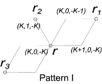
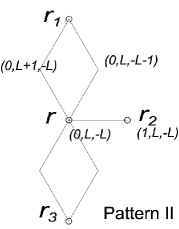
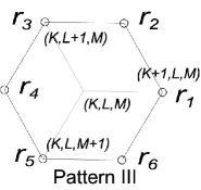
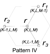
Figure 2: Equation patterns.

Theorem 3

Let the solution $z:Q_{H}\to{\mathbb{C}}$ of the system (1),(2) with initial data (4) be an immersion. Then function $r({\scriptscriptstyle K,L,M}):\tilde{Q}_{H}\to{{\mathbb{R}}_{+}}$, defined by (11), satisfies the following equations:

$$(r_{1}+r_{2})(r^{2}-r_{2}r_{3}+r(r_{3}-r_{2})\cos\alpha_{i})+(r_{3}+r_{2})(r^{2}-r_{2}r_{1}+r(r_{1}-r_{2})\cos\alpha_{i})=0$$ (13)

on the patterns of type I and II as in Fig.2, with $i=3$ and $i=2$ respectively,

$${\scriptstyle(L+M+1)}\frac{r_{4}-r_{1}}{r_{4}+r_{1}}+{\scriptstyle(M+K+1)}\frac{r_{6}-r_{3}}{r_{6}+r_{3}}+{\scriptstyle(K+L+1)}\frac{r_{2}-r_{5}}{r_{2}+r_{5}}=c-1$$ (14)

on the patterns of type III and

$$r(r_{1}\sin\alpha_{3}+r_{2}\sin\alpha_{1}+r_{3}\sin\alpha_{2})=r_{1}r_{2}\sin\alpha_{2}+r_{2}r_{3}\sin\alpha_{3}+r_{3}r_{1}\sin\alpha_{1}$$ (15)

on the patterns of type IV. Conversely, $r({\scriptscriptstyle K,L,M}):\tilde{Q}_{H}\to{{\mathbb{R}}_{+}}$ satisfying equations (13),(14),(15) is the radius function an immersed hexagonal circle pattern with constant intersection angles (i.e. corresponding to some immersed solution $z:Q_{H}\to{\mathbb{C}}$ of (1),(2)), which is determined by $r$ uniquely.

Proof: The map $z_{k,l,m}$ is an immersion if and only if all triangles $(z_{k,l,m},z_{k+1,l,m},z_{k,l,m-1})$,
$(z_{k,l,m},z_{k,l,m-1},z_{k,l+1,m})$ and $(z_{k,l,m},z_{k+1,l,m},z_{k,l+1,m})$ of elementary quadrilaterals of the map $z_{k,l,m}$ have the same orientation (for brevity we call it the orientation of the quadrilaterals).

Necessity: To get equation (14), consider the configuration of two star-like figures with centers at $z_{k,l,m}$ with $k+l+m=1\ ({\rm mod}\ 2)$ and at $z_{k+1,l,m}$, connected by five edges in the $k$-direction as shown on the left part of Fig.3.

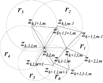
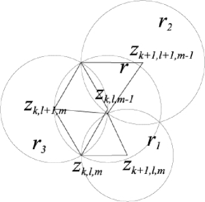
Figure 3: Circles.

Let $r_{i},\ i=1,...,6$ be the radii of the circles with the centers at the vertices neighboring $z_{k,l,m}$ as in Fig.3. As follows from Lemma 1, the vertices $z_{k,l,m}$, $z_{k+1,l,m}$ and $z_{k-1,l,m}$ are collinear. For immersed $z^{c}$, the vertex $z_{k,l,m}$ lies between $z_{k+1,l,m}$ and $z_{k-1,l,m}$. Similar facts are true also for the $l$- and $m$-directions. Moreover, the orientations of elementary quadrilaterals with the vertex $z_{k,l,m}$ coincides with one of the standard lattice. Lemma 1 defines all angles at $z_{k,l,m}$ of these quadrilaterals. Equation (2) at $(k,l,m)$ gives $z_{k,l,m}$:

$$z_{k,l,m}=\frac{2e^{is}}{c}\left(k\frac{r_{1}r_{4}}{r_{1}+r_{4}}+l\frac{r_{3}r_{6}}{r_{3}+r_{6}}e^{i(\alpha_{2}+\alpha_{3})}+m\frac{r_{2}r_{5}}{r_{2}+r_{5}}e^{i(\alpha_{1}+\alpha_{2}+2\alpha_{3})}\right),$$

where $e^{is}=(z_{k+1,l,m}-z_{k,l,m})/r_{1}$. Lemma 1 allows one to compute $z_{k+1,l,m-1}$, $z_{k+1,l+1,m}$, $z_{k+1,l,m+1}$ and $z_{k+1,l-1,m}$ using the form of quadrilaterals (they are shown in Fig. 3). Now equation (2) at $(k+1,l,m)$ defines $z_{k+2,l,m}$. Condition $|z_{k+2,l,m}-z_{k+1,l,m}|=r_{1}$ with the labels (12) yields equation (14).

For $l=0$ values $z_{k+1,0,m}$, $z_{k+2,0,m}$, $z_{k+1,0,m-1}$ and the equation for the cross-ratio with $\alpha_{3}$ give the radius $R$ with the center at $z_{k+2,0,m-1}$. Note that for $l=0$ the term with $r_{6}$ and $r_{5}$ drops out of equation (14). Using this equation and the permutation $R\to r_{1}$, $r_{1}\to r$, $r_{2}\to r_{2}$, $r_{5}\to r_{3}$, one gets equation (13) with $i=3$. The equation for pattern II is derived similarly.

To derive (15), consider the figure on the right part of Fig.3 where $k+l+m=1\ ({\rm mod}\ 2)$ and $r_{1}$, $r_{2}$, $r_{3}$ and $r$ are the radii of the circles with the centers at $z_{k+1,l,m}$, $z_{k+1,l+1,m-1}$, $z_{k,l+1,m}$ and $z_{k,l,m-1}$, respectively. Elementary geometrical considerations and Lemma 1 applied to the forms of the shown quadrilaterals give equation (15).

Remark. Equation (15) is derived for $r=r({\scriptscriptstyle K,L,M})$, $r_{1}=r({\scriptscriptstyle K,L,M-1})$, $r_{2}=r({\scriptscriptstyle K-1,L,M})$, $r_{3}=r({\scriptscriptstyle K,L-1,M+1})$. However it holds true also for $r_{1}=r({\scriptscriptstyle K,L,M+1})$, $r_{2}=r({\scriptscriptstyle K+1,L,M})$, $r_{3}=r({\scriptscriptstyle K,L+1,M+1})$ since it gives the radius of the circle through the three intersection points of the circles with radii $r_{1}$, $r_{2}$, $r_{3}$ intersecting at prescribed angles as shown in the right part of Fig.3. Later, we refer to this equation also for this pattern.

Sufficiency: Now let $r({\scriptscriptstyle K,L,M}):\tilde{Q}_{H}\to{\bf R_{+}}$ be some positive solution to (13),(14),(15). We can re-scale it so that $r({0,0,0})=1$. Starting with $r(1,0,-1)$ and $r(0,1,-1)$ one can compute $r$ everywhere in $\tilde{Q}_{H}$: $r$ in a ”black” vertex (see Fig.4) is computed from (14).

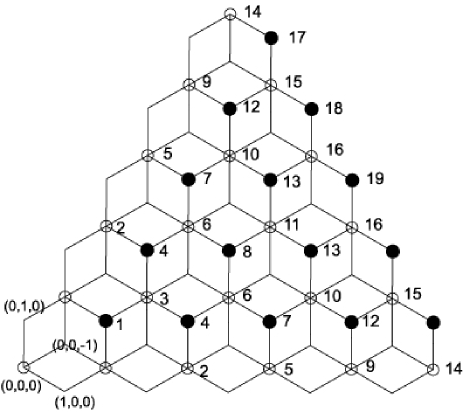
Figure 4: Computing $r$ in $\tilde{Q}_{H}$.

(Note that only $r$ at ”circled” vertices is used: so to compute $r_{1,1,-1}$ one needs only $r(1,0,-1)$ and $r(0,1,-1)$.) The function $r$ in ”white” vertices on the border $\partial\tilde{Q}_{H}=\{(K,0,-K)|K\in{\bf N}\}\cup\{(0,L,-L)|L\in{\bf N}\}$ is given by (13). Finally, $r$ in ”white” vertices in $Q^{int}_{H}=Q_{H}\setminus\partial\tilde{Q}_{H}$ is computed from (15). In Fig.4 labels show the order of computing $r$.

Lemma 2

Any solution $r({\scriptscriptstyle K,L,M}):\tilde{Q}_{H}\to{\bf R}$ to (13),(14),(15) with $0\leq c\leq 2$, which is positive for inner vertices of $\tilde{Q}_{H}$ defines some $z_{k,l,m}$ satisfying (1) in $Q$. Moreover, all the triangles $(z_{k,l,m},z_{k+1,l,m},z_{k,l,m-1})$, $(z_{k,l,m},z_{k,l,m-1},z_{k,l+1,m})$ and $(z_{k,l,m},z_{k+1,l,m},z_{k,l+1,m})$ have positive orientation.

Proof of the lemma: One can place the circles with radii $r({\scriptscriptstyle K,L,M})$ into the complex plane $\mathbb{C}$ in the way prescribed by the hexagonal combinatorics and the intersection angles. Taking the circle centers and the intersection points of neighboring circles, one recovers $z_{k,l,m}$ for $k+l+m=0,\pm 1$ up to a translation and rotation. Reversing the arguments used in the derivation of (13),(14),(15), one observes from the forms of the quadrilaterals that equations (1) are satisfied. Now using (1), one recovers $z$ in the whole $Q$. Equation (15) ensures that the radii $r$ remain positive, which implies the positive orientations of the triangles $(z_{k,l,m},z_{k+1,l,m},z_{k,l,m-1})$, $(z_{k,l,m},z_{k,l,m-1},z_{k,l+1,m})$ and $(z_{k,l,m},z_{k+1,l,m},z_{k,l+1,m})$.

Consider a solution $z:Q\to{\mathbb{C}}$ of the system (1),(2) with initial data (4), where $\phi$ and $\psi$ are chosen so that the triangles $(z_{0,0,0)},z_{1,0,0},z_{0,0,-1})$ and $(z_{0,0,0)},z_{0,0,-1},z_{0,1,0})$ have positive orientations and satisfy conditions $r(1,0,-1)=|z_{1,0,-1}-z_{1,0,0}|$ and $r(0,1,-1)=|z_{0,1,-1}-z_{0,0,-1}|$. The map $z_{k,l,m}$ defines circle pattern due to Proposition 1 and coincides with the map defined by Lemma 2 due to the uniqueness of the solution uniqueness. Q.E.D.

Since the cross-ratio equations and the constraint are compatible, the equations for the radii are also compatible. Starting with $r(0,0,0)$, $r(1,0,-1)$ and $r(0,1,-1)$, one can compute $r({\scriptscriptstyle K,L,M})$ everywhere in $\tilde{Q}$.

Lemma 3

Let a solution $r({\scriptscriptstyle K,L,M}):\tilde{Q}\to{\mathbb{R}}$ of (13),(14),(15) be positive in the planes given by equations $K+M=0$ and $L+M=0$ then it is positive everywhere in $\tilde{Q}$.

Proof: As follows from equation (15), $r$ is positive for positive $r_{i}$, $i=1,2,3.$ As $r$ at $(K,K,-K)$, $(K+1,K,-K-1)$ and $(K,K+1,-K-1)$ is positive, $r$ at $(K,K,K-1)$ is also positive. Now starting from $r$ at $(K,K,-K-1)$ and having $r>0$ at $(N,K+1,-K-1)$ and $(N,K,-K)$, one obtains positive $r$ at $(N,K,-K-1)$ for $0\leq N<K$ by the same reason. Similarly, $r$ at $(K,N,-K-1)$ is positive. Thus from positive $r$ at the planes $K+M=0$ and $L+M=0$, we get positive $r$ at the planes $K+M=-1$ and $L+M=-1$. Induction completes the proof.

Lemma 4

Let a solution $r({\scriptscriptstyle K,L,M}):\tilde{Q}\to{\mathbb{R}}$ of (13),(14),(15) be positive in the lines parameterized by $n$ as $(n,0,-n)$ and $(0,n,-n)$. Then it is positive in the border planes of $\tilde{Q}$ specified by $K+M=0$ and $L+M=0$.

Proof: We prove this lemma for $K+M=0$. For the other border plane it is proved similarly. Equation (14) for $(K,L,-K-1)$ gives

$$r_{2}=r_{5}\frac{(2L+c)r_{1}+(2K+c)r_{4}}{(2K+2-c)r_{1}+(2L+2-c)r_{4}}$$ (16)

therefore $r_{2}$ is positive provided $r_{1}$, $r_{5}$ and $r_{4}$ are positive. For $K=L$ it reads as

$$r_{2}=r_{5}\frac{(2K+c)}{(2K+2-c)}.$$ (17)

It allows us to compute recursively $r$ at $(K,K,-K)$ starting with $r$ at $(0,0,0)$. Obviously, $r>0$ for $(K,K,-K)$ if $r>0$ at $(0,0,0)$. This property together with the condition $r>0$ at $(n,0,-n)$ imply the conclusion of the lemma since equation (16) gives $r$ everywhere in the border plane of $\tilde{Q}$ specified by $K+M=0$.

Lemmas 3 and 4 imply that the circle pattern $z^{c}$ is an immersion if $r>0$ at $(N,0,-N)$ and $(0,N,-N)$.

4 Proof of the main theorem. Discrete Painlevé and Riccati equations

In this section, we prove that all $r(n,0,-n),\ \forall n\in{\mathbb{N}}$ are positive only for the initial data $z_{1,0,0}=1$, $z_{0,0,-1}=e^{c\alpha_{3}}$. For the line $r(0,n,-n)$ the proof is the same. Our strategy is as follows: first, we prove the existence of an initial value $z_{0,0,-1}$ such that $r(n,0,-n)>0,\ \forall n\in{\mathbb{N}}$, finally we will show that this value is unique and is $z_{0,0,-1}=e^{c\alpha_{3}}$.

Proposition 2

Suppose the equation

$$(n+1)(x_{n}^{2}-1)\left(\frac{x_{n+1}+{x_{n}}/{\varepsilon}}{\varepsilon+x_{n}x_{n+1}}\right)-n(1-{x_{n}^{2}}/{\varepsilon^{2}})\left(\frac{x_{n-1}+\varepsilon x_{n}}{\varepsilon+x_{n-1}x_{n}}\right)=cx_{n}\frac{\varepsilon^{2}-1}{2\varepsilon^{2}},$$ (18)

where $\varepsilon=e^{i\alpha_{3}}$, has a unitary solution $x_{n}=e^{i\beta_{n}}$ in the sector $0<\beta_{n}<\alpha_{3}$. Then $r(n,0,-n)$, $n\geq 0$ is positive.

Proof: For $z_{1,0,0}=1$ and unitary $z_{1,0,-1}$, the equation for the cross-ratio with $\alpha_{3}$ and (2) reduce to (18) with unitary $x_{n}^{2}=(z_{n,0,-n-1}-z_{n,0,n})/(z_{n+1,0,-n}-z_{n,0,n})$. Note that for $n=0$ the term with $x_{-1}$ drops out of (18); therefore the solution for $n>0$ is determined by $x_{0}$ only. The condition $0<\beta_{n}<\alpha_{3}$ means that all triangles $(z_{n,0,-n},z_{n+1,0,n},z_{n,0,-n-1})$ have positive orientation. Hence $r(n,0,-n)$ are all positive. Q.E.D.

Remark. Equation (18) is a special discrete Painlevé equation. For a more general reduction of cross-ratio equation see [19]. The case $\varepsilon=i$, corresponding to the orthogonally intersecting circles, was studied in detail in [2]. Here we generalize these results to the case of arbitrary unitary $\varepsilon$. Below we omit the index of $\alpha$ so that $\varepsilon=e^{i\alpha}$.

Theorem 4

There exists a unitary solution $x_{n}=e^{i\beta_{n}}$ to (18) in the sector $0<\beta_{n}<\alpha$.

Proof: Equation (18) allows us to represent $x_{n+1}$ as a function of $n,x_{n-1}$ and $x_{n}$: $x_{n+1}=\Phi(n,x_{n-1},x_{n})$. $\Phi(n,u,v)$ maps the torus $T^{2}=S^{1}\times S^{1}=\{(u,v)\in{\mathbb{C}}:\ |u|=|v|=1\}$ into $S^{1}$ and has the following properties:

• For all $n\in{\mathbb{N}}$ it is a continuous map on $A_{I}\times\bar{A}_{I}$ where $A_{I}=\{e^{i\beta}:\beta\in(0,\alpha)\}$ and $\bar{A}_{I}$ is the closure of $A_{I}$ . Values of $\Phi$ on the border of $A_{I}\times\bar{A}_{I}$ are defined by continuity: $\Phi(n,u,\varepsilon)=-1$, $\Phi(n,u,1)=-\varepsilon$.

• For $(u,v)\in A_{I}\times A_{I}$ one has $\Phi(n,u,v)\in A_{I}\cup A_{II}\cup A_{IV}$, where $A_{II}=\{e^{i\beta}:\beta\in(\alpha,\pi]\}$ and $A_{IV}=\{e^{i\beta}:\beta\in[\alpha-\pi,0)\}$. I.e., $x$ cannot jump in one step from $A_{I}$ into $A_{III}=\{e^{i\beta}:\beta\in(-\pi,\alpha-\pi)\}$.

Let $x_{0}=e^{i\beta_{0}}$. Then $x_{n}=x_{n}(\beta_{0})$. Define $S_{n}=\{\beta_{0}:\ x_{k}(\beta_{0})\in\bar{A}_{I}\ \forall\ 0\leq k\leq n\}$. Then $S_{n}$ is a closed set since $\Phi$ is continuous on $A_{I}\times\bar{A}_{I}$. As a closed subset of a segment it is a collection of disjoint segments $S_{n}^{l}$.

Lemma 5

There exists sequence $\{S_{n}^{l(n)}\}$ such that:

• $S_{n}^{l(n)}$ is mapped by $x_{n}(\beta_{0})$ onto $\bar{A}_{I}$,

• $S_{n+1}^{l(n+1)}\subset S_{n}^{l(n)}$.

The lemma is proved by induction. For $n=0$ it is trivial. Suppose it holds for $n$. As $S_{n}^{l(n)}$ is mapped by $x_{n}(\beta_{0})$ onto $\bar{A}_{I}$, continuity considerations and $\Phi(n,u,\varepsilon)=-1$, $\Phi(n,u,1)=-\varepsilon$ imply: $x_{n+1}(\beta_{0})$ maps $S_{n}^{l(n)}$ onto $A_{I}\cup A_{II}\cup A_{IV}$ and at least one of the segments $S_{n+1}^{l}\subset S_{n}^{l(n)}$ is mapped into $\bar{A}_{I}$. This proves the lemma.

Since the segments of $\{S_{n}^{l(n)}\}$ constructed in lemma 5 are nonempty, there exists $\bar{\beta}_{0}\in S_{n}$ for all $n\geq 0$. For this $\bar{\beta}_{0}$, the value $x_{n}(\bar{\beta}_{0})$ is not on the border of $\bar{A}_{0}$ since then $x_{n+1}(\beta_{0})$ would jump out of $\bar{A}_{I}$. Q.E.D..

Let $r_{n}$ and $R_{n}$ be the radii of the circles of the circle patterns defined by $z_{k,l,m}$ with the centers at $z_{2n,0,0}$ and $z_{2n+1,0,-1}$ respectively. Constraint (2) gives

$$r_{n+1}=\frac{2n+c}{2(n+1)-c}r_{n}$$

which is exactly formula (17). From elementary geometric considerations (see Fig. 5)

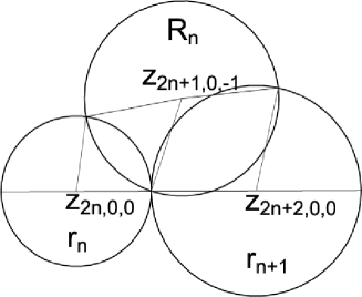
Figure 5: Circles on the border.

one gets

$$R_{n+1}=\frac{r_{n+1}-R_{n}\cos\alpha}{R_{n}-r_{n+1}\cos\alpha}r_{n+1}$$

(recall that $\alpha=\alpha_{3}$). Define

$$p_{n}=\frac{R_{n}}{r_{n}},\ \ \ g_{n}(c)=\frac{2n+c}{2(n+1)-c}$$

and denote $t=\cos\alpha$. Now, the equation for the radii $R,\ r$ takes the form:

$$p_{n+1}=\frac{g_{n}(c)-tp_{n}}{p_{n}-tg_{n}(c)}.$$ (19)

Remark. Equation (19) can be seen as a discrete version of a Riccati equation. This is motivated by the following properties:

• the cross-ratio of each four-tuple of its solutions is constant as $p_{n+1}$ is a Möbius transform of $p_{n}$,

• the general solution is expressed in terms of solutions of some linear equation: the standard Ansatz

  $$p_{n}=\frac{y_{n+1}}{y_{n}}+tg_{n}(c)$$ (20)

  transforms (19) into

  $$y_{n+2}+t(g_{n+1}(c)+1)y_{n+1}+(t^{2}-1)g_{n}(c)y_{n}=0.$$ (21)

As follows from Theorem 4, Proposition 2 and Lemma 4, equation (19) has a positive solution. One may conjecture that there is only one initial value $p_{0}$ such that $p_{n}>0,\ \forall n\in{\mathbb{N}}$ from the consideration of the asymptotics. Indeed, $g_{n}(c)\to 1$ as $n\to\infty$, and the general solution of equation (21) with limit values of coefficients is $y_{n}=c_{1}(-1)^{n}(1+t)^{n}+c_{2}(1-t)^{n}$. Thus $p_{n}=\frac{y_{n+1}}{y_{n}}+tg_{n}(c)\to-1$ for $c_{1}\neq 0$. However $c_{1},c_{2}$ define only the asymptotics of a solution. To relate it to the initial value $p_{0}$ is a more difficult problem. Fortunately, it is possible to find the general solution to (21).

Proposition 3

The general solution to (21) is

$$y_{n}=\frac{\Gamma(n+\frac{1}{2})}{\Gamma(n+1-\frac{c}{2})}(c_{1}\lambda_{1}^{n+1-c/2}F(\frac{3-c}{2},\frac{c-1}{2},\frac{1}{2}-n,z_{1})+$$ (22)

$$+c_{2}\lambda_{2}^{n+1-c/2}F(\frac{3-c}{2},\frac{c-1}{2},\frac{1}{2}-n,z_{2})$$

where $\lambda_{1}=-t-1,\ \lambda_{2}=1-t,\ z_{1}=(t-1)/2,\ z_{2}=-(1+t)/2$ and $F$ is the hypergeometric function.

Proof: The solution was found by a slightly modified symbolic method (see [11] for the method description and [4] for the detail). Here, $F(a,b,c,z)$ denotes the standard hypergeometric function which is a solution of the hypergeometric equation

$$z(1-z)F_{zz}+[c-(a+b+1)z]F_{z}-abF=0$$ (23)

holomorphic at $z=0$. Due to linearity, the general solution of (21) is given by a superposition of any two linearly independent solutions. Direct computation with the series representation of the hypergeometric function

$$F(1-\frac{\gamma-1}{2},\frac{\gamma-1}{2},1-\left(x+\frac{\gamma-1}{2}\right),z)=1+z\frac{(1-\frac{\gamma-1}{2})(\frac{\gamma-1}{2})}{(1-(x+\frac{\gamma-1}{2}))}+\ldots+$$ (24)

$$z^{k}\frac{\left[(1-\frac{\gamma-1}{2})(2-\frac{\gamma-1}{2})\ldots(k-\frac{\gamma-1}{2})\right]\left[(\frac{\gamma-1}{2})(1+\frac{\gamma-1}{2})\ldots(k-1\frac{\gamma-1}{2})\right]}{(1-(x\frac{\gamma-1}{2}))\ldots(k-(x+\frac{\gamma-1}{2}))}+\ldots$$

shows that each summand in (22) satisfies equation (21). To finish the proof of Proposition 3, one has to show that the particular solutions with $c_{1}=0,\ c_{2}\neq 0$ and $c_{1}\neq 0,\ c_{2}=0$ are linearly independent. This fact follows from

Lemma 6

As $n\to\infty$, function (22) has the asymtotics

$$y_{n}\simeq(n+1-\gamma/2)^{\frac{\gamma-1}{2}}(c_{1}\lambda_{1}^{n+1-\gamma/2}+c_{2}\lambda_{2}^{n+1-\gamma/2}).$$ (25)

For $n\to\infty$ the series representation (24) implies $F(\frac{3-\gamma}{2},\frac{\gamma-1}{2},\frac{1}{2}-n,z_{1})\simeq 1$. Stirling’s formula

$$\Gamma(x)\simeq\sqrt{2\pi}e^{-x}x^{x-\frac{1}{2}}$$ (26)

yields the asymptotics of the factor $\frac{\Gamma(n+\frac{1}{2})}{\Gamma(n+1-\frac{\gamma}{2})}$. This completes the proof of the lemma and of Proposition (3).

Proposition 4

A solution of the discrete Riccati equation (19) with $\alpha\neq\pi/2$ is positive for all $n\geq 0$ if and only if

$$p_{0}=\frac{\sin\frac{c\alpha}{2}}{\sin\frac{(2-c)\alpha}{2}}.$$ (27)

Proof: For positive $p_{n}$, it is necessary that $c_{1}=0$: this follows from asymptotics (25) substituted into (20). Let us define

$$s(z)=1+z\frac{(1-\frac{\gamma-1}{2})(\frac{\gamma-1}{2})}{\frac{1}{2}}+\ldots+z^{k}\frac{(k-\frac{\gamma-1}{2})\ldots(1-\frac{\gamma-1}{2})(\frac{\gamma-1}{2})(k-1+\frac{\gamma-1}{2})}{k!(k-\frac{1}{2})\ldots\frac{1}{2}}\ldots$$ (28)

This is the hypergeometric function $F(\frac{3-\gamma}{2},\frac{\gamma-1}{2},\frac{1}{2}-n,z)$ with $n=0$. A straightforward computation with series shows that

$$p_{0}=1+\frac{2(\gamma-1)}{2-\gamma}z+\frac{4z(z-1)}{2-\gamma}\frac{s^{\prime}(z)}{s(z)}$$ (29)

where $z=\frac{1+t}{2}$. Note that $p_{0}$ as a function of $z$ satisfies an ordinary differential equation of first order since $\frac{s^{\prime}(z)}{s(z)}$ satisfies the Riccati equation obtained by a reduction of (23). A computation shows that $\frac{\sin\frac{\gamma\alpha}{2}}{\sin\frac{(2-\gamma)\alpha}{2}}$ satisfies the same ordinary differential eqiation. Since both expression (29) and (27) are equal to 1 for $z=0$, they coincide everywhere. Q.E.D.

Proof of Theorem 1: Proposition (4) implies that the initial $x_{0}$ for which (18) gives positive $r$ is unique and implies the initial values (5) for $z^{c}$ if $\alpha_{i}\neq\pi/2$. For the case $\alpha=\pi/2$, any solution for (19) with $p_{0}>0$ is positive. Nevertheless, as was proved in [2], $x_{0}$ is in this case also unique and is specified by (27). Thus for all $n\in{\mathbb{N}}$ we have $r(n,0,-n)>0$, $r(0,n,-n)>0$ for the circle pattern $z^{c}$. Lemmas 4 and 3 complete the proof.

5 Hexagonal circle patterns $z^{2}$ and $\rm Log$

For $c=2$, formula (17) gives infinite $r(1,1,-1)$. The way around this difficulty is renormalization $z\to(2-c)z/c$ and a limit procedure $c\to 2-0$, which leads to the re-normalization of initial data (see [9]). As follows from (27), this renormalization implies:

$$r(0,0,0)=0,\ r(1,0,-1)=\frac{\sin\alpha_{3}}{\alpha_{3}},\ r(0,1,-1)=\frac{\sin\alpha_{2}}{\alpha_{2}},\ r(1,1,-1)=1.$$ (30)

Proposition 5

The solution to (13),(14),(15) with $c=2$ and initial data (30) is positive.

Proof: This follows from Lemmas 3 and 4 since Theorem 4 is true also for the case $c=2$. Indeed, solution $x_{n}$ is a continuous function of $c$. Therefore it has a limit value as $c\to 2-0$ and it lies in the sector $A_{I}$.

Lemma 2 implies that there exists a hexagonal circle pattern with radius function $r$.

Definition 3

The hexagonal circle pattern $Z^{2}$ has a radius function specified by Proposition 5.

Equations (13),(14),(15) have the symmetry

$$r\to\frac{1}{r},\ c\to 2-c,$$ (31)

which is the duality transformation (see [10]). The smooth analog $f\to f^{*}$ for holomorphic functions $f(w),f^{*}(w)$ is:

$$\frac{df(w)}{dw}\frac{df^{*}(w)}{dw}=1.$$

Note that ${\rm log}^{*}(w)=w^{2}/2$. The hexagonal circle pattern $\rm Log$ is defined [9] as a circle pattern dual to $Z^{2}$. Discrete $z^{2}$ and $\rm Log$ are the first two images in Fig. 6.

Theorem 5

The hexagonal circle patterns $Z^{2}$ and $\rm Log$ are immersions.

Proof: For $z^{2}$ this follows from Proposition 5. Hence the values of $1/r$, where $r$ is radius function for $z^{2}$, are positive except for $r(0,0,0)=\infty$. Lemma 2 completes the proof.

6 Concluding remarks

In this section we discuss corollaries of the obtained results and possible generalizations.

6.1 Square grid circle patterns $z^{c}$ and $\rm Log$

Equations (1) extend $z_{k,l,m}$ corresponding to the hexagonal $z^{2}$ and $\rm Log$ from $Q_{H}$ into the three-dimensional lattice $Q$. The $r$-function of this extension satisfies equation (15). Consider $z_{k,l,m}$ for the hexagonal $z^{c}$ and $\rm Log$ restricted to one of the coordinate planes, e.g. $l=0$. Then Proposition 1 states that $z_{k,0,m}$ defines some circle pattern with combinatorics of the square grid: each circle has four neighboring circles intersecting it at angles $\alpha_{3}$ and $\pi-\alpha_{3}$. It is natural to call it square grid $z^{c}$ (see the third image in Fig. 6). Such circle patterns are natural generalization of those with orthogonal neighboring and tangent half-neighboring circles introduced and studied in [22].

Theorem 6

Square grid $z^{c}$, $0<c\leq 2$ and $\rm Log$ are immersions.

Proof easily follows from lemma 2.

Figure 6: Hexagonal $z^{2}$, $\rm Log$ and square grid $z^{3/2}$.

It is interesting to note that the square grid circle pattern $z^{c}$ can be obtained from hexagonal one by limit procedure $\alpha_{3}\to+0$ and by $\alpha_{1}\to\pi-\alpha_{2}$. These limit circle patterns still can be defined by (1), (2) by imposing the self-similarity condition $z_{k,l,m}=f_{l,k-m}$.

6.2 Square grid circle patterns $\rm Erf$

For square grid combinatorics and $\alpha=\pi/2$, Schramm [22] constructed circle patterns mimicking holomorphic function ${\rm erf}(z)=(2/\pi)\int e^{-z^{2}}dz$ by giving the radius function explicitly. Namely, let $n,m$ label the circle centers so that the pairs of circles $c(n,m)$, $c(n+1,m)$ and $c(n,m)$, $c(n,m+1)$ are orthogonal and the pairs $c(n,m)$, $c(n+1,m+1)$ and $c(n,m+1)$, $c(n+1,m)$ are tangent. Then

$$r(n,m)=e^{nm}$$ (32)

satisfies the equation for a radius function:

$$R^{2}(r_{1}+r_{2}+r_{3}+r_{4})-(r_{2}r_{3}r_{4}+r_{1}r_{3}r_{4}+r_{1}r_{2}r_{4}+r_{1}r_{2}r_{3})=0,$$ (33)

where $R=r(n,m)$, $r_{1}=r(n+1,m)$, $r_{2}=r(n,m+1)$, $r_{3}=r(n-1,m)$, $r_{4}=r(n,m-1)$. For square grid circle patterns with intersection angles $\alpha$ for $c(n,m)$, $c(n+1,m)$ and $\pi-\alpha$ for $c(n,m)$, $c(n,m+1)$ the governing equation (33) becomes

$$R^{2}(r_{1}+r_{2}+r_{3}+r_{4})-(r_{2}r_{3}r_{4}+r_{1}r_{3}r_{4}+r_{1}r_{2}r_{4}+r_{1}r_{2}r_{3})+2R\cos\alpha(r_{1}r_{3}-r_{2}r_{4})=0.$$ (34)

It is easy to see that (34) has the same solution (32) and it therefore defines a square grid circle pattern, which is a discrete $\rm Erf$. A hexagonal analog of $\rm Erf$ is not known.

6.3 Circle patterns with quasi-regular combinatorics.

One can deregularize the prescribed combinatorics by a projection of ${\mathbb{Z}}^{n}$ into a plane as follows (see [23]). Consider ${{\mathbb{Z}}^{n}_{+}}\subset{\mathbb{R}}^{n}$. For each coordinate vector ${\bf e}_{i}=(e^{1}_{i},...,e^{n}_{i})$, where $e^{j}_{i}=\delta^{j}_{i}$ define a unit vector ${\bf\xi}_{i}$ in ${\mathbb{C}}={\mathbb{R}}^{2}$ so that for any pair of indices $i,j$, vectors ${\bf\xi}_{i},{\bf\xi}_{j}$ form a basis in ${\mathbb{R}}^{2}$. Let $\Omega\in{\mathbb{R}}^{n}$ be some 2-dimensional simply connected cell complex with vertices in ${\mathbb{Z}}^{n}_{+}$. Choose some ${x_{0}}\in\Omega$. Define the map $P:\Omega\to{\mathbb{C}}$ by the following conditions:

• $P(x_{0})=P_{0}$,

• if $x,y$ are vertices of $\Omega$ and $y=x+{\bf e}_{i}$ then $P(y)=P(x)+{\bf\xi}_{i}$.

It is easy to see that $P$ is correctly defined and unique.
We call $\Omega$ a projectable cell complex if its image $\omega=P(\Omega)$ is embedded, i.e. intersections of images of different cells of $\Omega$ do not have inner parts. Using projectable cell complexes one can obtain combinatorics of Penrose tilings.

It is natural to define “discrete conformal map on $\omega$” as a discrete complex immersion function $z$ on vertices of $\omega$ preserving the cross-ratios of the $\omega$-cells. The argument of $z$ can be labeled by the vertices $x$ of $\Omega$. Hence for any cell of $\Omega$, constructed on ${\bf e}_{k},{\bf e}_{j}$, the function $z$ satisfies the following equation for the cross-ratios:

$$q(z_{x},z_{x+{\bf e_{k}}},z_{x+{\bf e_{k}}+{\bf e_{j}}},z_{x+{\bf e_{j}}})=e^{-2i\alpha_{k,j}},$$ (35)

where $\alpha_{k,j}$ is the angle between ${\bf\xi}_{k}$ and ${\bf\xi}_{j}$, taken positively if $({\bf\xi}_{k},{\bf\xi}_{j})$ has positive orientation and taken negatively otherwise. Now suppose that $z$ is a solution to (35) defined on the whole ${\mathbb{Z}}^{n}_{+}$. We can define a discrete $z^{c}:\omega\to{\mathbb{C}}$ for projectable $\Omega$ as a solution to (35),(36) restricted to $\Omega$. Initial conditions for this solution are of the form (5) so that the restrictions of $z$ to each two-dimensional coordinate lattice is an immersion defining a circle pattern with prescribed intersection angles. This definition naturally generalizes the definition of discrete hexagonal and square grid $z^{c}$ considered above.

We finish this section with the natural conjecture formulated in [4].

Conjecture. The discrete $z^{c}:\omega\to{\mathbb{C}}$ is an immersion.

First step in proving this claim is to show that equation (35) is compatible with the constraint

$$cf_{x}=\sum_{s=1}^{n}2x_{s}\frac{(f_{x+{\bf e}_{s}}-f_{x})(f_{x}-f_{x-{\bf e}_{s}})}{f_{x+{\bf e}_{s}}-f_{x-{\bf e}_{s}}}$$ (36)

For $n=3$ this fact is proven in [9].

7 Acknowledgements

This research was supported by the DFG Research Center ”Mathematics for key technologies” (FZT 86) in Berlin and the EPSRC grant No Gr/N30941.

References

- [1]
- [2] S.I.Agafonov, A.I.Bobenko, Discrete and Painlevé equations, Internat. Math. Res. Notices, 4 (2000), 165-193
- [3] S.I.Agafonov, Embedded circle patterns with the combinatorics of the square grid and discrete Painlevé equations, Discrete Comput. Geom., 29:2 (2003), 305-319
- [4] S.I.Agafonov, Discrete Riccati equation, hypergeometric functions and circle patterns of Schramm type, Preprint arXiv:math.CV/0211414
- [5] A.F.Beardon, T.Dubejko, K.Stephenson, Spiral hexagonal circle packings in the plane, Geom. Dedicata, 49 (1994), 39-70
- [6] A.F.Beardon, K.Stephenson The uniformization theorem for circle packings, Indiana Univ. Math. J., 39:4 (1990), 1383-1425
- [7] A.I.Bobenko, T.Hoffmann, Conformally symmetric circle packings. A generalization of Doyle spirals, Experimental Math., 10:1 (2001), 141-150
- [8] A.I.Bobenko, T.Hoffmann, Yu.B.Suris, Hexagonal circle patterns and integrable systems: Patterns with the multi-ratio property and Lax equations on the regular triangular lattice, Internat. Math. Res. Notices, 3 (2002), 111-164.
- [9] A.I.Bobenko, T.Hoffmann, Hexagonal circle patterns and integrable systems. Patterns with constant angles, to appear in Duke Math. J., Preprint arXiv:math.CV/0109018
- [10] A. Bobenko, U. Pinkall, Discretization of surfaces and integrable systems, In: Discrete Integrable Geometry and Physics; Eds. A.I.Bobenko and R.Seiler, pp. 3-58, Oxford University Press, 1999.
- [11] G. Boole, Calculus of finite differences, Chelsea Publishing Company, NY 1872.
- [12] K. Callahan, B. Rodin, Circle packing immersions form regularly exhaustible surfaces, Complex Variables, 21 (1993), 171-177.
- [13] T.Dubejko, K.Stephenson, Circle packings: Experiments in discrete analytic function theory, Experimental Math. 4:4, (1995), 307-348
- [14] Z.-X. He, O. Schramm, The convergence of hexagonal disc packings to Riemann map, Acta. Math. 180 (1998), 219-245.
- [15] Z.-X. He, Rigidity of infinite disk patterns, Annals of Mathematics 149 (1999), 1-33.
- [16] T. Hoffmann, Discrete CMC surfaces and discrete holomorphic maps, In: Discrete Integrable Geometry and Physics, Eds.: A.I.Bobenko and R.Seiler, pp. 97-112, Oxford University Press, 1999.
- [17] A.Marden, B.Rodin, On Thurston’s formulation and proof of Andreev’s theorem, pp. 103-115, Lecture Notes in Math., Vol. 1435, 1990.
- [18] F. Nijhoff, H. Capel, The discrete Korteveg de Vries Equation, Acta Appl. Math. 39 (1995), 133-158.
- [19] F.W. Nijhoff, Discrete Painlevé equations and symmetry reduction on the lattice. In: Discrete Integrable Geometry and Physics; Eds. A.I.Bobenko and R.Seiler, pp. 209-234, Oxford University Press, 1999.
- [20] B. Rodin, Schwarz’s lemma for circle packings, Invent. Math., 89 (1987), 271-289.
- [21] B. Rodin, D. Sullivan, The convergence of circle packings to Riemann mapping, J. Diff. Geometry 26 (1987), 349-360.
- [22] O. Schramm, Circle patterns with the combinatorics of the square grid, Duke Math. J. 86 (1997), 347-389.
- [23] M. Senechal, Quasicrystals and geometry. Cambridge University Press, Cambridge, 1995.
- [24] W.P. Thurston, The finite Riemann mapping theorem, Invited talk, International Symposium on the occasion of the proof of the Bieberbach Conjecture, Purdue University (1985).