The Honeycomb Problem on the Sphere

Abstract.

The honeycomb problem on the sphere asks for the partition of the sphere into $N$ equal areas that minimizes the perimeter. This article solves the problem when $N=12$. The unique minimizer is a tiling of $12$ regular pentagons in the dodecahedral arrangement.

1. Introduction

The classical honeycomb problem asks for the perimeter-minimizing partition of the plane into regions of equal area. The optimal solution is the regular hexagonal honeycomb tiling. This article adapts the planar proof to partitions on the unit sphere. The honeycomb problem on the sphere asks for the perimeter-minimizing partition of the sphere into $N$ equal areas. This article solves the problem when $N=12$. The unique minimizer is a tiling of $12$ regular pentagons in the dodecahedral arrangements. This problem was solved by L. Fejes Tóth, under an assumption of convexity in [4].

2. The hexagonal isoperimetric inequality

The honeycomb theorem in the plane follows by showing that the regular hexagon is the unique minimizer of a particular functional on the set of closed curves with finitely many marked points. This section gives a review of this result. It is the result that will be generalized in this article.

Let $\Gamma$ be a closed piecewise simple rectifiable curve in the plane. We use the parameterization of the curve to give it a direction, and use the direction to assign a signed area to the bounded components of the plane determined by the curve. For example, if $\Gamma$ is a piecewise smooth curve, the signed area is given by Green’s formula

$$\int_{\Gamma}xdy.$$

Generally, we view $\Gamma$ as an integral current [11, p.44]. We let $P$ be an integral current with boundary $\Gamma$. Expressed differently, we give a signed area by assigning an multiplicity $m(U)\in\mathbb{Z}$ to each bounded component $U$ of $\mathbb{R}^{2}\setminus\Gamma$. (An illustration appears in Figure 1.) The area is $\sum m(U){\operatorname{area}}(U)$. $P$ is represented by the formal sum $P=\sum m(U)U$.

Let $v_{1},\ldots,v_{t}$, $t\geq 2$, be a finite list of points on $\Gamma$. We do not assume that the points are distinct. Index the points $v_{1},v_{2},\ldots,v_{t}$, in the order provided by the parameterization of $\Gamma_{i}$. Join $v_{i}$ to $v_{i+1}$ by a directed line segment $f_{i}$ (take $v_{t+1}=v_{1}$). The chords $f_{i}$ form a generalized polygon, and from the direction assigned to the edges, it has a signed area $A_{P}\in\mathbb{R}$.

Figure 1. Signed areas in the plane.

Let $e_{i}$ be the segment of $\Gamma$ between $v_{i}$ to $v_{i+1}$. Let $f^{{\operatorname{op}}}$ be the chord $f$ with the orientation reversed. Let $x(e_{i})\in\mathbb{R}$ be the signed area of the integral current bounded by $(e_{i},f_{i}^{{\operatorname{op}}})$. Let $E(P)=\{e_{i}\}$ denote the set of edges of $P$. Accounting for multiplicities and orientations, we have

$${\operatorname{area}}(P)=A_{P}+\sum_{e\in E(P)}x(e).$$

Let $\alpha(P)=\min(1,{\operatorname{area}}(P))$.

Define a truncation function $\tau:\mathbb{R}\to\mathbb{R}$ by

$$\tau(x)=\begin{cases}1/2,&x\geq 1/2,\\ x,&|x|\leq 1/2,\\ -1/2,&x\leq-1/2.\end{cases}$$

Set $T(P)=\sum_{E(P)}\tau(x(e))$. Recall that the perimeter of a regular hexagon of unit area is $2{\root 4 \of{1}2}$. Let $L(P)$ be the length of $\Gamma$. Let $N(P)$ be the number of points $v_{i}$ on $\Gamma$, counted with multiplicities. Let $a(N)=\min(2\pi\sqrt{3}/(3N^{2}),1)$. The following is proved in [9].

Theorem 1.

(hexagonal isoperimetric inequality) Define $P$, $L(P)$, $N(P)$, and $a(N)$ as above. Assume that the signed area of $P$ is at least $a(N(P))$. Then

$$L(P)\geq-T(P){\root 4 \of{1}2}-(N(P)-6)0.0505+2\alpha(P){\root 4 \of{1}2}.$$

Equality is attained if and only if $P$ is a regular hexagon of area 1.

3. The pentagonal isoperimetric inequality

We adapt the inequality of Theorem 1 to pentagons on the unit sphere.

The first important difference as we move from the plane to the sphere is that a simple closed curve bounds two simply connected regions. A parameterized simple closed curved can be viewed as giving a positive orientation to one of the regions and a negative orientation to the other. It is not generally clear which area is to be preferred. This ambiguity disappears if we take all areas on the sphere to be defined modulo multiples of $4\pi$. Thus, we define the area bounded by a closed curve as taking values in $\mathbb{R}/(4\pi\mathbb{Z})$. If a parameterized curve bounds an area $A\in\mathbb{R}/(4\pi\mathbb{Z})$, then the oppositely parameterized curve bounds an area $-A$. A representative in $\mathbb{R}$ for a constant in $\mathbb{R}/(4\pi\mathbb{Z})$ will be called a real representative. We define ${\operatorname{mrr}}:\mathbb{R}/(4\pi\mathbb{Z})\to\mathbb{Z}$ (the minimal real representative) to be the function taking each $x$ to the real representative in $[-2\pi,2\pi)$.

We will also make use of the unsigned area of regions, which is the usual Lebesgue measure of a region taking values in the set of non-negative real numbers. Write ${\operatorname{unsigned}}(R)$ for the unsigned area of a region $R$.

Let $\Gamma$ be a closed piecewise simple rectifiable curve on the unit sphere.

As before, let $v_{1},\ldots,v_{t}$, $t\geq 2$, be a finite list of points on $\Gamma$. We do not assume that the points are distinct. Index the points $v_{1},v_{2},\ldots,v_{t}$, in the order provided by the parameterization of $\Gamma$. Join $v_{i}$ to $v_{i+1}$ by an arc $f_{i}$ of a great circle. (The choice of arc will be fixed in a moment.) Take $v_{t+1}=v_{1}$. Let $P$ be an integral current with boundary $\Gamma$. The chords $f_{i}$ form a generalized polygon, and from the direction assigned to the edges, it has a signed area $A_{P}\in\mathbb{R}/(4\pi\mathbb{Z})$.

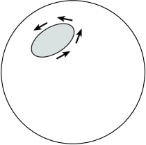
Figure 2. Signed areas on the unit sphere. The two regions have signed areas $\epsilon$ and $-4\pi+\epsilon$

Let $e_{i}$ be segment of $\Gamma$ between $v_{i}$ to $v_{i+1}$. Let $f^{{\operatorname{op}}}$ be the chord $f$ with the orientation reversed. Let $x(e_{i})\in\mathbb{R}/(4\pi\mathbb{Z})$ be the signed area of the integral current bounded by $(e_{i},f_{i}^{{\operatorname{op}}})$.

If $v_{i}$ and $v_{i+1}$ are antipodal, there are infinitely many geodesic arcs $f_{i}$ joining $v_{i}$ and $v_{i+1}$. In this case, choose $f_{i}$ in such a way that $x(e_{i})=0$. If $v_{i}$ and $v_{i+1}$ are not antipodal, then these two points break the great circle through them into two circular arcs $f^{\prime}$ and $f^{\prime\prime}$. There is a difference of $2\pi$ between the signed area of the integral current bounded by $(e_{i},f^{\prime{\operatorname{op}}})$ and that bounded by $(e_{i},f^{\prime\prime{\operatorname{op}}})$. We choose $f_{i}=f^{\prime}$ or $f^{\prime\prime}$ in a way to make $x(e_{i})$ have its minimal real representative in $[-\pi,\pi)$.

Let $E(P)=\{e_{i}\}$ denote the set of edges of $P$. Accounting for multiplicities and orientations, we have

$${\operatorname{area}}(P)=A_{P}+\sum_{e\in E(P)}x(e)\in\mathbb{R}/(4\pi\mathbb{Z}).$$

We emphasize that this identity does not hold in general between the minimal real representatives of the terms.

Define a truncation function $\tau:\mathbb{R}/(4\pi\mathbb{Z})\to\mathbb{R}$ by

$$\tau(x)=\begin{cases}0.32,&{\operatorname{mrr}}(x)\geq 0.32,\\ {\operatorname{mrr}}(x),&|{\operatorname{mrr}}(x)|\leq 0.32,\\ -0.32,&{\operatorname{mrr}}(x)\leq-0.32\end{cases}$$

Set $\tau_{0}=0.32$. Set $T(P)=\sum_{E(P)}\tau(x(e))$.

Let ${\operatorname{reg-perim}}:\mathbb{R}/(4\pi\mathbb{Z})\times\mathbb{N}\to\mathbb{R}$ be the function that gives the perimeter of a regular spherical $n$-gon of area $x$. It satisfies

$${\operatorname{reg-perim}}(-x,n)={\operatorname{reg-perim}}(x,n).$$

The perimeter of a regular spherical pentagon in the tiling by $12$ pentagons is

$${\operatorname{reg-perim}}(\pi/3,5)\approx 3.64864.$$

Let $p_{5}$ equal this constant.

The function ${\operatorname{reg-perim}}$ is given explicitly by the following Mathematica module.

regPerim[area_, n_] := Module[{cosgamma, alpha},
    alpha = Pi - (2Pi - area)/n;
    cosgamma = (Cos[2Pi/n] + Cos[alpha/2]^2)/Sin[alpha/2]^2;
    n ArcCos[cosgamma]
    ]

The derivation is a simple calculation based on spherical trigonometry (the spherical law of cosines) and Figure 3. From this explicit formula, we see that ${\operatorname{reg-perim}}(\pi/3,n)$ extends to an analytic function of $n>0$. Let $p^{\prime}_{5}$ be the partial derivative $\partial_{2}{\operatorname{reg-perim}}(\pi/3,5)$.

Figure 3. The triangulation used to compute ${\operatorname{reg-perim}}$.

Let ${\operatorname{circ-perim}}:[0,2\pi)\times\mathbb{R}/(4\pi\mathbb{Z})\to\mathbb{R}$ be defined as follows. Let $\ell\in[0,2\pi)$ be the length of an arc of a great circle on the unit sphere. Draw a circle on the unit sphere passing through the two endpoints of the arc with the property that one of the two areas bounded by the arc and the circle has signed area $x$. Let ${\operatorname{circ-perim}}(\ell,x)$ be the length of the part of the circle between the two endpoints that (together with the arc) bounds the region of area $x$. For example,

$${\operatorname{circ-perim}}(0,x)$$

is the perimeter of a circle of area $x$. Explicitly,

(1) $${\operatorname{circ-perim}}(0,x)=\sqrt{4\pi x-x^{2}}.$$

(Compare [13, Eqn 10.1].) To give another example,

$${\operatorname{circ-perim}}(\pi,x)=\pi,$$

because in this case, the two endpoints of the arc are antipodal and the circle must be a great circle through the antipodal points.

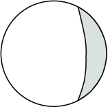
Figure 4. The arc of the circle bounding the shaded region has length ${\operatorname{circ-perim}}$.

Let

$${\operatorname{pent}}(x)={\operatorname{circ-perim}}({\operatorname{reg-perim}}(\pi/3-x,5)/5,|x|/5)5$$

It equals the perimeter of a regular pentagon of area $\pi/3$ in which the geodesic edges have been replaced by arcs of a circle. When $x>0$ the edges bulge outward and when $x<0$, the edges bulge inward. See Figure 5. Because of the absolute value in the formula, it is not obvious that this is differentiable at $x=0$. Nevertheless, it turns out to be, and we set

$$B^{\prime}={\operatorname{pent}}^{\prime}(0).$$

A calculation shows in fact that

$$B^{\prime}=-\partial_{1}{\operatorname{reg-perim}}_{1}(\pi/3,5)\approx-1.51.$$

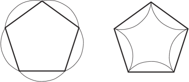
Figure 5. ${\operatorname{pent}}(x)$ is the perimeter of bulging pentagon. The heavy set geodesic pentagon has area $\pi/3-x$ and each of the five two-sided regions has area $|x|/5$.

Let $L(P)$ be the length of $\Gamma$. Let $N(P)$ be the number of points $v_{i}$ on $\Gamma$, counted with multiplicities. Let

$$a(N)=\min(3.75/n^{2},0.1).$$

Let

$$\rho(P)=\begin{cases}3\,|{\operatorname{mrr}}({\operatorname{mrr}}(P))|/\pi&\text{if }0\leq|{\operatorname{mrr}}({\operatorname{area}}(P))|\leq\pi/3,\\ 1&\text{otherwise.}\end{cases}$$

Theorem 2.

(Isoperimetric inequality for spherical pentagons) Define $P$, $L(P)$, $N(P)$, $a(N)$, $\rho(N)$, $p_{5}$, $p_{5}^{\prime}$, and $B^{\prime}$ as above. Assume that

$${\operatorname{mrr}}({\operatorname{area}}(P))\in(a(N(P)),2\pi).$$

Then

$$L(P)\geq T(P)B^{\prime}-(5-N(P))p_{5}^{\prime}+\rho(P)p_{5}.$$

Equality is attained if and only if $P$ is a regular spherical pentagon of unsigned area $\pi/3$, so that $L(P)=p_{5}$, $T(P)=0$, $N(P)=5$, and $\rho(P)=1$.

4. The proof of the main result

This section assumes Theorem 2 and derives the main result from it. The following section will give a proof of the isoperimetric inequality.

Theorem 3.

($12$ honeycombs on a sphere) Let $R_{1},\ldots,R_{12}$ be a partition of the unit sphere into $12$ measurable sets of equal area $(\pi/3)$. Let $h={\mathcal{H}}^{1}(\cup\{R_{1},\ldots,R_{12}\})$ be the $1$-dimensional Hausdorff measure of the current boundary. Then

$$h\geq 6\,{\operatorname{reg-perim}}(\pi/3,5).$$

If equality is attained, then up to a set of $1$-dimensional Hausdorff measure zero, the current boundary is equal to the perimeter of the tiling by $12$ congruent regular spherical pentagons.

In preparation for the proof, we let $R_{1},\ldots,R_{12}$ be a minimizer of the $1$-dimensional Hausdorff boundary subject to the constraints that each area is $\pi/3$. A minimizer exists by [10]. The theorem is stated for planar soap bubbles; but the proof carries through without difficulty to a sphere.

By the results of [10], we may assume various regularity results. Each $R_{i}$ is an open region bounded by finitely many analytic arcs. The collection of arcs meet one another only at their endpoints. The number of arcs meeting at each endpoint is two or three. Call this the degree of the endpoint. Each $R_{i}$ consists of finitely many connected components and each connected component is connected and simply connected. Each connected component $P$ has a finite number of marked points $N(P)$, determined by the endpoints of arcs of degree three. Each connected component has at least one marked point.

Orient each region by the outward normal on the sphere, so that each signed area ${\operatorname{area}}(P)$ is positive and equal to the Lebesgue measure of $R_{i}$.

Since the dodecahedral tiling has perimeter $6\,{\operatorname{reg-perim}}(\pi/3,5)$, the minimizer has a perimeter no greater than this constant.

Lemma 4.

In an optimal configuration, the total unsigned area of the connected components of unsigned area at most $0.1$ is less than $4.0$.

Proof.

Each connected component of unsigned area $x\in(0,0.1]$ gives a perimeter at least ${\operatorname{circ-perim}}(0,x)$. The function has negative second derivative so that the perimeter is at least

$$x\,{\operatorname{circ-perim}}(0,0.1)/0.1.$$

Each segment of perimeter is shared by at most two such regions. Thus, if the total area is at least $4.0$, the total perimeter is at least

$$4.0\,{\operatorname{circ-perim}}(0,0.1)/0.2>6\,{\operatorname{reg-perim}}(\pi/3,5),$$

contrary to the supposed optimality of the perimeter. ∎

Assume for a contradiction that we have found a strict contradiction to the theorem, that is, a partition into equal areas with perimeter strictly less than $6\,{\operatorname{reg-perim}}(\pi/3,5)$. Write this in the form

(2) $$\sum_{i}({\operatorname{perim}}(R^{\prime}_{i})-\rho_{i}p_{5})<0,$$

where the sum extends over connected components $R^{\prime}_{i}$, and the area fractions $\rho_{i}$ are at most $1$ and sum to $12$.

We repeatedly modify the set of connected components by picking a connected component of unsigned area at most $a(N)$, and deleting the edge segments shared with another region. This decreases the number of connected components by one. We continue until all regions satisfy the lower bound $a(N)$. The regions before this process had areas at most $\pi/3$. After the process, because of the lemma, each region $R_{i}^{\prime\prime}$ has area less than $\pi/3+4.0<2\pi$.

In the previous paragraph we always delete the edge segments with the region that causes the perimeter to decrease the most. Some edge segment has length at least $1/N$ times the perimeter, where $N$ is the number of junctures of degree $3$. The perimeter, by the isoperimetric inequality for spheres [13], is at most ${\operatorname{circ-perim}}(0,x)$ (that is, the perimeter of a circle of area $x$). Thus, the perimeter decreases by at least ${\operatorname{circ-perim}}(0,x)/N$, where $x=\rho_{i}\pi/3\leq a(N)$.

The sum $\sum_{i}\rho_{i}$ is unaffected by merging the two regions (say with indices $1$ and $2$) if $\rho_{1}+\rho_{2}\leq 1$; that is, $\rho^{\prime}_{1}=\rho_{1}+\rho_{2}$, $\rho_{2}^{\prime}=0$. But the sum can decrease if $\rho_{1}+\rho_{2}>1$; that is, $\rho^{\prime}_{1}=1$, $\rho_{2}^{\prime}=0$, and $\rho_{1}+\rho_{2}\neq\rho_{1}^{\prime}+\rho_{2}^{\prime}$. Overall, the left-hand side of Inequality 2 is at most what is was originally plus the term

$$-2{\operatorname{circ-perim}}(0,\rho_{i}\pi/3)/N+\rho_{i}p_{5}\leq-2{\operatorname{circ-perim}}(0,|x|)/N+3|x|p_{5}/\pi.$$

This term is always non-positive by the inequality $|x|\leq a(N)$ and the explicit formula (1). It is zero iff $x=0$. Hence, a counterexample remains a counterexample even after the edge deletion process. We drop the primes in notation, and consider Inequality 2 as applying to a partition of the sphere that has no areas less than $a(N)$.

It is shown in [9] that configuration can be modified so that it is still a counterexample, but so that every region is connected and simply connected, and so that the degree at every marked point is $3$. We make this modification here too.

Inequality 2 can be rewritten as

$$\sum_{P}\left[(L(P)-T(P)B^{\prime}+(5-N(P))p_{5}^{\prime}-\rho(P)p_{5}\right]<0.$$

This uses the Euler relation

$$\sum_{P}(N(P)-5)=0$$

and the skew symmetry of $\tau$:

$$\sum_{P}T(P)=0.$$

In this form, it is clear that the inequality contradicts the isoperimetric inequality for pentagons. This proves that there is no perimeter strictly less than $6\,{\operatorname{reg-perim}}(\pi/3,5)$.

Assume that we have a perimeter equal to $6\,{\operatorname{reg-perim}}(\pi/3,5)$. As before, we may assume that the boundaries of the regions are analytic arcs. No edges are deleted in the edge-deletion process, because such would lead to a strict inequality. Thus, all areas area at least $a(N)$ and we can apply the pentagonal isoperimetric inequalities to conclude that each region is a regular pentagon of area $\pi/3$. This concludes the proof.

5. Proof of the isoperimetric inequality

This section gives a proof of the isoperimetric inequality stated in Section 3. The proof is similar to the proof of the hexagonal isoperimetric inequality in [9].

Estimate 5.

If a region has unsigned area $x\leq 2\pi$, the perimeter is at least ${\operatorname{circ-perim}}(0,x)$.

Proof.

This is the isoperimetric inequality on a sphere, which can be deduced from the methods of [13]. ∎

Estimate 6.

If an $n$-gon has unsigned area $x$ at most $2\pi$, the perimeter is at least ${\operatorname{reg-perim}}(x,n)$.

Proof.

This is [8, Lemma 6.1]. ∎

We also use Dido’s theorem for a unit sphere.

Theorem 7.

(Dido) Let $R$ be a region of area $x$ at most $\pi$ on the unit sphere bounded by a great circle and some other curve $C$. The length of $C$ is at least that of a semicircle meeting the great circle at right angles and enclosing an area $x$.

That is, the length is at least ${\operatorname{circ-perim}}(0,2x)/2$.

Proof.

This follows easily from the isoperimetric inequality. ∎

Lemma 8.

If $0\leq x\leq y<4\pi$, then

$$y\,{\operatorname{circ-perim}}(0,x)\geq x\,{\operatorname{circ-perim}}(0,y).$$

Proof.

This is an elementary consequence of the explicit Formula (1). ∎

Lemma 9.

If $x\in[0.03,2.33]$ and $n\in[3,4,5,6,7]$, then

$$\partial_{1}^{2}{\operatorname{reg-perim}}(x,n)<0.$$

Proof.

This is an interval arithmetic calculation based on the explicit formula for ${\operatorname{reg-perim}}$. If $f$ is a function, the Mathematica procedure to check that its second derivative is negative on $[a,a+nw]$ is three lines of code (listed below). The result is thus readily checked (with $w=1/1000$). ∎

maxSecond[f_,a_,n_,w_]:= Module[{i,der2},
    der2 = D[f[x],{x,2}];
    Table[der2/.{x->Interval[{a+i w,a+(i+1)w}]},{i,0,n-1}]//Max
    ];

Let

$$I(\ell,n,t,\rho)=\ell-tB^{\prime}+(5-n)p_{5}^{\prime}-\rho p_{5}.$$

To prove the pentagonal isoperimetric inequality, we wish to show that $I(L(P),N(P),T(P),\rho(P))$ is non-negative. Let $x_{i}=x(e_{i})$ and $t_{i}=\tau(x_{i})$, and $T_{{\operatorname{abs}}}=\sum|t_{i}|$. Let $\ell_{i}=L(e_{i})$. Recall that $|t_{i}|\leq\tau_{0}$.

We consider several cases. In each successive case, we may assume that at least one of the defining conditions of the previous cases fail. A common technique will be to reflect one arc of the perimeter $\Gamma$ in such a way that the area increases (but not beyond $2\pi$) and the perimeter remains the same length. Using the negativity of the second derivative of ${\operatorname{circ-perim}}$ and ${\operatorname{reg-perim}}$, most of the cases reduce to checking that the inequality is satisfied at the endpoints of its domain.

5.1. Case $n\geq 5$ and $T_{{\operatorname{abs}}}\geq 1.301$.

Recall that we have chosen $x_{i}$ so that $|x_{i}|\leq\pi$, so that Dido’s theorem applies. In this case, the inequality follows because the lemma gives

$$\ell_{i}\geq|t_{i}|{\operatorname{circ-perim}}(0,2\tau_{0})/(2\tau_{0})$$

so that

$$I\geq I(5,1.301\,{\operatorname{circ-perim}}(0,2\tau_{0})/(2\tau_{0}),-1.301,1)>0.$$

We now assume that $T_{{\operatorname{abs}}}<1.301$.

5.2. Case $n\geq 5$ and ${\operatorname{area(P)}}\geq 3.474$

By the previous case, $|T(P)|\leq T_{{\operatorname{abs}}}<1.301$. Then

$$I\geq I(5,{\operatorname{circ-perim}}(0,3.474),-1.301,1)>0.$$

From now on, we assume that if $n\geq 5$, then we have ${\operatorname{area(P)}}<3.474$.

5.3. Case $n\geq 5$ and some $x_{i}>\tau_{0}$

If some $x_{i}>\tau_{0}$ and some $x_{j}<-\tau_{0}$, we may shrink both bounding curves to decrease $|x_{i}|$, $|x_{j}|$, and $L(P)$, while fixing $T(P)$ and ${\operatorname{area}}(P)$. This decreases $I$ and transforms any counterexample to a counterexample. If some $x_{j}<-\tau_{0}$ we may shrink the bounding curve $L(P)$ to increase $x_{j}$ and ${\operatorname{area}}(P)$, while maintaining $T(P)$. This again transforms counterexamples to counterexamples. If ${\operatorname{area}}(P)$ ever increases to $3.474$, we are done by the earlier case. Thus, we may assume that all $x_{j}\geq-\tau_{0}$.

Assume some $x_{i}>\tau_{0}$. Let $t_{neg}=\sum_{i}\min(0,t_{i})$. We have $T(P)\geq\tau_{0}+t_{neg}$. Since $x_{i}\geq-\tau_{i}$, we have $\sum_{i}\min(0,x_{i})=t_{neg}$. If we reflect each negative area $x_{i}$ about the segment $f_{i}$ then $P$ is transformed into a region $P^{\prime}$ of area ${\operatorname{area}}(P)+2|t_{neg}|\geq\rho(P)\pi/3+2|t_{neg}|$. The area of $P^{\prime}$ is at most $3.474+2(1.301)<2\pi$, so that it falls within the monotonic range of ${\operatorname{circ-perim}}$. We have

$$I\geq I(5,{\operatorname{circ-perim}}(0,\rho\pi/3+2|t_{neg}|),\tau_{0}-|t_{neg}|,\rho).$$

The function on the right is positive for all $\rho\in[0,1]$ and all $|t_{neg}|\in[0,1.301]$, as the explicit formula 1 readily shows.

From now on, we assume that if $n\geq 5$, then we have $x_{i}\leq\tau_{0}$ for all $i$. Thus, $x_{i}=t_{i}$. If some $t_{i}<0$ and another $t_{j}>0$, we may shrink the bounding curve while maintaining $t_{i}+t_{j}$ and area. This transformation takes counterexamples to counterexamples. Thus, we may assume that all $t_{i}$ have the same sign.

5.4. Case $n=5$, $\rho\geq 0.9957$, $T(P)\in[-0.0711,0.117]$, and some edge $f_{i}$ has arc-length at least $1$.

Lemma 10.

Let $P$ be a spherical pentagon of area $x<2\pi$ on the unit sphere. Assume that it has an edge of arclength at least $1$. If the regular pentagon of area x has edges of arclength at least $1$, then that pentagon is perimeter minimizing. Otherwise the perimeter minimizer is that with edges $1$, $u,u,u,u$ inscribed in a circle. (See Figure 6.)

Figure 6. Perimeter Minimizer with a long edge. Four edges have length $u$ and the top edge has length $1$. The angles at the origin are $\alpha$, $\beta$, $\beta$, $\beta$, $\beta$. The arclength of the radius is $x$. Also, the angle $\gamma$ is that along the isosceles triangle with base $1$ and $\delta$ is that along the isosceles triangle with base $u$.

Proof.

The case of $5$ equal edge lengths has already been considered. Let us assume that the edge constraint rules out the regular pentagon. The proof of [8, Lemma 6.1] shows that the optimal solution will have edge $1$, $u$, $u$, $u$, $u$, for some $u$.

The argument that the optimal figure will have a circumscribing circle is classical, at least in the analogous case of the plane. In [7], it is shown that the optimal polygon among equilateral polygons is the regular polygon. Their argument actually shows that for any three consecutive equilateral sides, the two interior angles along the middle segment are equal. This implies that the pentagon will have equal angles at vertices at the end of two edges of length $u$. For a pentagon, this is sufficient to give a circumscribing circle. ∎

By simple spherical trig (the law of cosines), the perimeter and area of this pentagon are described parametrically in terms of the arclength $x$ of the radius of the circle. This gives the following parametric equations for perimeter and area.

perimArea[x_]:= Module[{beta,alpha,u,gamma,delta,perim,area},
    alpha = ArcCos[(Cos[1] - Cos[x]^2)/(Sin[x]^2)];
    beta = (2 Pi - alpha)/4;
    u = ArcCos[Sin[x]^2 Cos[beta] + Cos[x]^2];
    gamma = ArcCos[(Cos[x]-Cos[x] Cos[1])/(Sin[x] Sin[1])];
    delta = ArcCos[(Cos[x]-Cos[x] Cos[u])/(Sin[x] Sin[u])];
    perim = 1 + 4 u;
    area = (alpha + 2 gamma - Pi) + 4 (beta+ 2delta - Pi);
    {perim,area}
    ];

The signed area bounded by the generalized polygon with segments $f_{i}$ is at least $\rho\pi/3-T(P)$, so that $T(P)\geq\rho\pi/3-{\operatorname{area}}_{x}$. This gives

(3) $$I\geq I(5,{\operatorname{perim}}_{x},\rho\pi/3-{\operatorname{area}}_{x},\rho)\geq I(5,{\operatorname{perim}}_{x},\pi/3-{\operatorname{area}}_{x},1)$$

The perimeter is increasing in $x$, for $x\leq\pi/2$. Clearly $x\geq 0.5$. If $x>0.7$, then ${\operatorname{perim}}_{x}>3.8$ and

$$I\geq I(5,3.8,-0.0711,1)>0.$$

The area is increasing in $x$, for $x\leq 0.7$. If $x<0.6$, then

$$0.92<0.9957\pi/3-0.117\leq\rho\pi/3-T(P)\leq{\operatorname{area}}_{x}<0.82.$$

This contradiction shows that we may assume $x\in[0.6,0.7]$. For $x\in[0.6,0.7]$, the right-hand side of Inequality 3 is positive, as an easy calculation shows.

5.5. Case $n=5$, $\rho\geq 0.9957$, $T(P)\in[-0.0711,0.117]$

This subsection follows the proof of the hexagonal honeycomb conjecture closely. See [9, Sec. 8]. By the isoperimetric inequality, we may assume that all edges $e_{i}$ are arcs of circles. We may assume that each arc has the same curvature by [10, Thm 2.3, step 3]. Following [9, Prop. 6.1], the perimeter is at least

$$\begin{array}[]{lll}&{\operatorname{circ-perim}}(1,|t|/{\operatorname{reg-perim}}(\rho\pi/3-t,5)){\operatorname{reg-perim}}(\rho\pi/3-t,5)\\ &\qquad\qquad\leq{\operatorname{circ-perim}}(1,|t|/3.65){\operatorname{reg-perim}}(\rho\pi/3-t,5).\end{array}$$

Let $C(\rho,t)$ be the right-hand side of this inequality. We have

$$I\geq I(5,C(\rho,t),t,\rho).$$

The right-hand side is non-negative. We first use interval arithmetic to prove positivity outside the set

$$\{(\rho,t):\rho\in[0.999,1]\quad t\in[-0.04,0.043]\}.$$

Then the $\rho$-derivative is shown to be negative by another interval arithmetic calculation, and this reduces the problem to $\rho=1$. Yet another interval calculation reduces the problem to the interval

$$t\in[-0.005,0.005].$$

Finally an interval calculation shows that the second derivative with respect to $t$ is strictly positive for $t\in[-0.005,0.005]$. All of these calculations were made with Mathematica’s interval function and a few lines of code. Exact arithmetic shows that the function is zero and has zero derivative at $t=0$. Thus, $t=0$ is the unique minimizer. Equality is achieved iff $\rho=1$ and $t=0$. In this case, we have a regular pentagon of area $\pi/3$.

From here on, we assume that if $n=5$, we have $\rho\leq 0.9957$ or $T(P)\not\in[-0.0711,0.117]$.

5.6. Case $n\geq 5$, $T(P)\geq 0$

Define $\rho_{1}$ by

$$\rho_{1}(n)=\begin{cases}0.913&n=5\\ 0.952&n=6\\ 0.99&n=7\\ 1.0&n\geq 8.\end{cases}$$

Define $T_{1}$ by

$$T_{1}(n)=\begin{cases}0.117&n=5\\ 0.065&n=6\\ 0.0134&n=7\end{cases}$$

For $\rho\leq\rho_{1}(n)$, we find that

$$I\geq I(n,{\operatorname{circ-perim}}(0,\rho\pi/3),0,\rho)>0$$

by the explicit formula for ${\operatorname{circ-perim}}$.

Assume $\rho>\rho_{1}(n)$. For $T(P)\geq T_{1}(N(P))$ we have

$$I\geq I(n,{\operatorname{circ-perim}}(0,\rho\pi/3),t,\rho)>0,$$

as we can readily check by looking at the endpoints of functions with negative second derivatives.

Assume $\rho\geq\rho_{1}(n)$ and $T(P)\in[0,T_{1}(N(P))]$. We have reduced to the case $N(P)\in[5,6,7]$. If $N(P)=5$, we assume that $\rho\leq 0.9957$. We have

$$I\geq I(n,{\operatorname{reg-perim}}(\rho\pi/3-t,n),t,\rho)>0$$

by checking endpoints and using a second derivative test.

5.7. Case $n\geq 5$, $T(P)\leq 0$

Define $T_{0}$ by

$$T_{0}(n)=\begin{cases}-0.1382&n=5\\ -0.0711&n=6\\ -0.01362&n=7\\ 0&n\geq 8.\end{cases}$$

Assume that $T(P)\in[-1.301,T_{0}(n)]$. We have

$$I\geq I(n,{\operatorname{circ-perim}}(0,\rho\pi/3-2t),t,\rho)>0$$

by a second-derivative test.

Assume that $T(P)\in[T_{0}(n),0]$. We may also assume $n<8$. Define $\rho_{2}$ by

$$\rho_{2}(n)=\begin{cases}0.913&n=5\\ 0.952&n=6\\ 0.99&n=7.\end{cases}$$

If we also assume $\rho\in[0,\rho_{2}(N(P))]$, we find that

$$I\geq I(n,{\operatorname{circ-perim}}(0,\rho\pi/3-2t),t,\rho)>0.$$

Assuming that $\rho\in[\rho_{2}(n),0.9957]$ when $n=5$, and $\rho\in[\rho_{2}(n),1]$ otherwise, we have

$$I\geq I(n,{\operatorname{reg-perim}}(\rho\pi/3-t,n),t,\rho)>0$$

for all $T\in[T_{0}(n),0]$ by a second derivative test.

We have now completed the proof of the pentagonal isoperimetric inequality for $n\geq 5$.

5.8. Case $n=4$

This case is similar to the case $n\geq 5$. We simply list the differences. Note that $T(P)=\sum^{4}t_{i}\geq-4\tau_{0}$. If $T(P)>0.168$, use

$$I\geq I(4,{\operatorname{circ-perim}}(0,\rho\pi/3),0.168,\rho)>0.$$

If some area $|x_{i}|$, $|A_{P}|$, or $|{\operatorname{area}}(P)|$ has minimal real representative between $3.56$ and $4\pi-3.56$, then

(4) $$I\geq I(4,{\operatorname{circ-perim}}(0,3.56),-4\tau_{0},1)>0.$$

If some $x_{i}>\tau_{0}$, we contract the boundary as before to assume that $x_{j}\geq-\tau_{0}$ for all $i$. Reflecting the region corresponding to each $t_{j}<0$, we add $2|t_{j}|$ to the area. The area increases by at most $2\tau_{0}$ to at most $3.56+2\tau_{0}$. If this is greater than $3.56$, it is less than $2\pi$, and the area estimate (4) applies. Thus, we may assume after each reflection that the new area is less than $3.56$. We obtain

$$I\geq I(4,{\operatorname{circ-perim}}(0,\rho\pi/3+2|t_{neg}|,\tau_{0}-|t_{neg}|,\rho).$$

The right-hand-side is positive for $\rho\in[0,1]$ and $|t_{neg}|\in[0,3\tau_{0}]$.

As above, we may assume that $x_{i}\in[-\tau_{0},\tau_{0}]$. Recall that $a(4)=0.1$. We finish the case $n=4$ with several estimates.

$$I\geq I(4,{\operatorname{circ-perim}}(\rho\pi/3),t,\rho)>0,$$

if $\rho\in[0.1,0.85]$ and $t\in[0,0.168]$.

$$I\geq I(4,{\operatorname{reg-perim}}(\rho\pi/3-t,4),t,\rho)>0,$$

if $\rho\in[0.85,1]$ and $t\in[0,0.168]$.

$$I\geq I(4,{\operatorname{circ-perim}}(\rho\pi/3-2t),t,\rho)>0$$

if $\rho\in[0.1,0.85]$ and $t\in[-4\tau_{0},0]$, or if $\rho\in[0.1,1]$ and $t\in[-4\tau_{0},-0.25]$.

$$I\geq I(4,{\operatorname{reg-perim}}(\rho\pi/3-t,4),t,\rho)>0$$

if $\rho\in[0.85,1]$ and $t\in[-0.25,0]$.

5.9. Case $n=3$

This case is similar to $n=4$. If $T(P)>0.22$, we use an estimate like that of Section 5.8. The proof is the same if we modify the constants in the proof as follows:

$$\begin{array}[]{lll}-0.25\mapsto-0.35,&3.56\mapsto 2.84,&0.168\mapsto 0.22,\\ 4\mapsto 3,&3\mapsto 2,&0.85\mapsto 0.8.\end{array}$$

5.10. Case $n=2$, Great Circle

There are two types of digons. We call them great circle digons or simple arc digons. Recall that we choose $x_{i}$ so that its minimal real representative lies in the interval $[-\pi,\pi)$. A choice of arc $f_{i}$ of a great circle was chosen for each edge $e_{i}$ to make the minimal real representatives lie in the given interval. In the case of a digon the two arcs $f_{1}$ and $f_{2}$ have the same endpoints. If the endpoints are the two parts of a great circle then we have a great circle digon. If the arcs trace the same path with opposite orientations then we have a simple arc digon. These two types are shown in Figure 7.

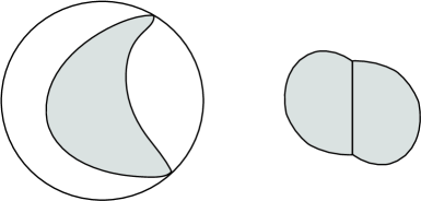
Figure 7. Two types of digons.

Assume we have a great circle digon. We have $|A_{P}|=2\pi$, $x_{1},x_{2}\in[-\pi,0]$, and $|x_{1}|+|x_{2}|+|{\operatorname{area}}(P)|=2\pi$.

If the area of the digon is at least $2.29$, we have

(5) $$I\geq I(2,{\operatorname{circ-perim}}(0,2.29),-2\tau_{0},1)>0.$$

We claim that if the unsigned area $|{\operatorname{area}}(P)|$ of the digon is in $[\pi/3,2.29]$, then the area increases to a value in $[2.29,4\pi-2.29]$, upon reflection of the region represented by $x_{1}$ (Figure 8). This implies that $I>0$ by Inequality 5. In fact, after reflection, the area is at most

$$|{\operatorname{area(P)}}|+2|x_{1}|\leq 2.29+2\pi<4\pi-2.29.$$

Recall that

$$|x_{1}|=2\pi-|{\operatorname{area}}(P)|-|x_{2}|\geq 2\pi-2.29-\pi=\pi-2.29.$$

Hence, the area is at least

$$|{\operatorname{area}}(P)|+2|x_{1}|\geq\pi/3+2(\pi-2.29)>2.29.$$

Figure 8. Reflection on a digon region.

Finally, suppose that the unsigned area of the digon is at most $\pi/3$. In this case, we again reflect the areas represented by $x_{1}$. We have

$$|x_{1}|=2\pi-|{\operatorname{area}}(P)|-|x_{2}|\geq 2\pi-\pi/3-\pi=2\pi/3.$$

So the reflected area $R_{A}$ satisfies

$$2.29<2|x_{1}|\leq R_{A}\leq\pi/3+2\pi<4\pi-2.29.$$

Hence, we may again apply Inequality 5. This completes the case of great circle digons.

5.11. Case $n=2$, Simple Arc

In this case, $A_{P}=0$ and the signed area is simply $x_{1}+x_{2}$.

If $T(P)\geq 0.271$, then the result follows from

$$I\geq I(2,{\operatorname{circ-perim}}(0,\rho\pi/3),0.271,\rho)>0.$$

Assume that $T(P)\leq 0.271$.

If the area is between $2.29$ and $2\pi$, we may apply Inequality 5 to prove that $I>0$. Assume that the area is less than $2.29$.

If some $x_{i}<-\tau_{0}$ contract the perimeter increasing $x_{i}$ and the area $x_{1}+x_{2}$ until either the area becomes $2.29$ or $x_{i}\geq-\tau_{0}$. Assume now that $x_{i}\geq-\tau_{0}$.

If some $x_{i}>\tau_{0}$ contract the perimeter while decreasing $x_{1}+x_{2}$ until either $x_{i}=\tau_{0}$ or $x_{1}+x_{2}\leq\pi/3$. Assume $x_{1}+x_{2}\leq\pi/3$. We have

$$T(P)=\tau_{0}+t_{\min}\leq 0.271$$

and

$$x_{\min}\leq t_{\min}\leq 0.271-\tau_{0}=-0.049.$$

Reflecting $x_{\min}$, we have

$$I\geq I(2,{\operatorname{circ-perim}}(0,\rho\pi/3+2|t_{\min}|),\tau_{0}-|t_{\min}|,\rho)>0,$$

for $|t_{\min}|\in[0.049,\tau_{0}]$ and $\rho\in[0,1]$.

If $x_{1},x_{2}\in[-\tau_{0},\tau_{0}]$ and they have opposite signs, we may contract the perimeter while maintaining $x_{1}+x_{2}=t_{1}+t_{2}$, until they have the same sign.

Finally, assume that $x_{1},x_{2}\in[-\tau_{0},\tau_{0}]$ and that they have the same sign.

$$0.271\geq T(P)=t_{1}+t_{2}=x_{1}+x_{2}=|{\operatorname{area}}(P)|\geq 0,$$

so the sign is positive. Assume that $\rho\geq a(2)=0.1$ (as allowed by the hypothesis of the pentagonal isoperimetric inequality). We have

$$I\geq I(2,{\operatorname{circ-perim}}(0,\rho\pi/3),\rho\pi/3,\rho)>0,$$

for $\rho\in[0.1,1]$.

6. Concluding Remarks

The method of the honeycomb conjecture is seen to extend to the spherical case. As a further test of the generality of the method, it would be interesting to see whether the method can be used to prove the corresponding results for $N=3$, $4$, and $6$ regions of equal area. A further test of the method would be to extend it to the honeycomb problem in the hyperbolic plane. I am not aware of any obstructions to doing so.

My motivation for pursuing the case of a sphere is that for

$$N\neq 1,2,3,4,6,12,$$

the optimal solution will not consist of congruent regular polygons. The study of these irregular cases can lead us to valuable insights into problems such as the Kelvin problem, where the best known solution contains two types of cells. As a preliminary step, it is necessary to develop the spherical theory at a level comparable to what has been done for the plane. That is the purpose of these calculations.

References

- [1] F. J. Almgren, Jr. Existence and regularity of almost everywhere of solutions to elliptic variational problems with constraints, Mem. AMS, 165 (1976).
- [2] C. Cox, L. Harrison, M. Hutchings, S. Kim, J. Light, A. Mauer, M. Tilton, The shortest enclosure of three connected areas in , Real Analysis Exchange, Vol. 20(1), 1994/95, 313–335.
- [3] H. Federer, Geometric Measure Theory, Springer-Verlag, 1969.
- [4] L. Fejes Tóth, Über das kürzeste Kurvennetz das eine Kugeloberfläche in flächengleiche konvexe Teil zerlegt, Mat. Term.-tud. Értesitö 62 (1943), 349–354.
- [5] L. Fejes Tóth, Regular Figures, MacMillan Company, 1964.
- [6] L. Fejes Tóth, What the bees know and what they do not know, Bulletin AMS, Vol 70, 1964.
- [7] W. Habicht and B. L. van der Waerden, Lagerung von Punkten auf der Kugel, Math. Ann. 123 (1951) 223-234.
- [8] T. C. Hales, The sphere packing problem, J. Comp. and Appl. Math. 44 (1992) 41–76.
- [9] T. C. Hales, The honeycomb conjecture, Discr. Comput. Geom. 25:1-22 (2001).
- [10] F. Morgan, Soap bubbles in and in surfaces, Pacific J. Math, 165 (1994), no. 2, 347–361.
- [11] F. Morgan, Geometric Measure Theory, A Beginner’s Guide, Second Edition, Academic Press, 1995.
- [12] F. Morgan, The hexagonal honeycomb conjecture, Trans. AMS, Vol 351, Number 5, pages 1753–1763, 1999.
- [13] F. Morgan, The Isoperimetric Problem on Surfaces, Amer. Math. Monthly, vol 106, 5, May 1999, 430–439.
- [14] J. Taylor, The structure of singularities in soap-bubble-like and soap-film-like minimal surfaces, Annals of Math., 103 (1976), 489-539.