Combining Kernel Estimators in
the Uniform Deconvolution Problem

Abstract

We construct a density estimator and an estimator of the distribution function in the uniform deconvolution model. The estimators are based on inversion formulas and kernel estimators of the density of the observations and its derivative. Initially the inversions yield two different estimators of the density and two estimators of the distribution function. We construct asymptotically optimal convex combinations of these two estimators. We also derive pointwise asymptotic normality of the resulting estimators, the pointwise asymptotic biases and an expansion of the mean integrated squared error of the density estimator. It turns out that the pointwise limit distribution of the density estimator is the same as the pointwise limit distribution of the density estimator introduced by Groeneboom and Jongbloed (2003), a kernel smoothed nonparametric maximum likelihood estimator of the distribution function.
AMS classification: primary 62G05; secondary 62E20, 62G07, 62G20
Keywords: uniform deconvolution, kernel estimation, asymptotic normality

1 Introduction

Consider the general deconvolution model. Let $X_{1},\ldots,X_{n}$ be i.i.d. observations, where $X_{i}=Y_{i}+Z_{i}$ and $Y_{i}$ and $Z_{i}$ are independent. Assume that the unobservable $Y_{i}$ have distribution function $F$ and density $f$. Also assume that the unobservable random variables $Z_{i}$ have a known density $k$. Note that the density $g$ of $X_{i}$ is equal to the convolution of $f$ and $k$, so $g=k*f$ where $*$ denotes convolution. So we have

$$g(x)=\int_{-\infty}^{\infty}k(x-u)f(u)du.$$ (1)

The deconvolution problem is the problem of estimating $f$ or $F$ from the observations $X_{i}$. Later on we will restrict ourselves to uniform deconvolution where we require the distribution of the $Z_{i}$ to be uniform.

Several generally applicable methods have been proposed for this deconvolution model but let us review direct kernel density estimation first. Consider estimation of the density function $g$ from the observations $X_{1},\cdots,X_{n}$. The kernel density estimator with kernel function $w$ and bandwidth $h>0$, is defined by

$$g_{nh}(x)=\frac{1}{n}\,\sum_{j=1}^{n}\frac{1}{h}\,w\Big{(}\frac{x-X_{j}}{h}\Big{)}.$$ (2)

For smooth $g$, essentially twice continuously differentiable, and symmetric $w$ with integral one, we have

$${\rm E\,}g_{nh}(x)=\int_{-\infty}^{\infty}\frac{1}{h}\,w\Big{(}\frac{x-u}{h}\Big{)}g(u)du$$

$$\quad=g(x)+\frac{1}{2}\,h^{2}g^{\prime\prime}(x)\int u^{2}w(u)du+o(h^{2}),$$

$$\mathop{\rm Var}\nolimits g_{nh}(x)=\frac{1}{nh}\,g(x)\int w^{2}(u)du+o\Big{(}\frac{1}{nh}\Big{)},$$

as $n\to\infty,h\to 0$ and $nh\to\infty$. For more on direct kernel density estimators see for instance Prakasa Rao (1983), Silverman (1986) and Wand and Jones (1995).

The standard Fourier type kernel density estimator for deconvolution problems is based on the Fourier transform. For an introduction see for instance Wand and Jones (1995). Let $w$ denote a kernel function and $h>0$ a bandwidth. The estimator $f_{nh}(x)$ of the density $f$ at the point $x$ is defined as

$$f_{nh}(x)=\frac{1}{2\pi}\int_{-\infty}^{\infty}e^{-itx}\frac{\phi_{w}(ht)\phi_{emp}(t)}{\phi_{k}(t)}\,dt={1\over nh}\sum_{j=1}^{n}v_{h}\Big{(}{{x-X_{j}}\over h}\Big{)},$$

with

$$v_{h}(u)={1\over 2\pi}\int_{-\infty}^{\infty}{{\phi_{w}(s)}\over\phi_{k}(s/h)}\ e^{-isu}ds,$$

where

$$\phi_{emp}(t)={1\over n}\sum_{j=1}^{n}e^{itX_{j}},$$

and $\phi_{w}$ and $\phi_{k}$ denote the characteristic functions of $w$ and $k$ respectively.

An important condition for these estimators to be properly defined is that the characteristic function $\phi_{k}$ of the density $k$ has no zeroes, which renders it useless for instance for uniform deconvolution. At the same time this shows that uniform deconvolution is a non standard deconvolution problem. In fact, Hu and Ridder (2004) argue that in economic applications the assumption of no zeros for $\phi_{k}$ is not reasonable. If the error distribution has bounded support and is symmetric then its characteristic function will have zeros. They propose an approximation of the Fourier transform estimator in such cases. For other modifications of the Fourier inversion method, applicable to uniform deconvolution, see Hall and Meister (2007) and Feuerverger, Kim and Sun (2008).

A second general approach is nonparametric maximum likelihood. The likelihood of $F$ is equal to

$$\prod_{j=1}^{n}g(X_{j})=\prod_{j=1}^{n}\int_{-\infty}^{\infty}k(X_{j}-t)dF(t).$$

One can try to explicitly determine a distribution function $F$ that maximizes this likelihood. This works for exponential deconvolution where a unique explicit maximizing $F$ can be derived, see Jongbloed (1998). For a special case of uniform deconvolution (if the distribution induced by $F$ concentrated on [0,1]) an explicit expression for a maximizing $F$ can also be derived. However, from formula (3) below it follows that the likelihood is determined by the values $F(X_{j})-F(X_{j}-1),i=j,\ldots,n$. Hence any $F$ assigning the same probability to the intervals $(X_{j}-1,X_{j}]$ will have the same likelihood. So here the maximizer is not unique. In other cases a numerical maximization procedure is required. For recent results see the thesis of S. Donauer.

A third general approach is provided by inversion. A selected group of deconvolution problems allows explicit inversion formulas of (1), expressing the density of interest $f$ in terms of the density $g$ of the data. In these cases we can estimate $f$ by substituting for instance a direct density estimate of $g$, for instance the kernel estimate (2), in the inversion formula. In Van Es and Kok (1998) this strategy has been pursued for deconvolution problems where $k$ equals the exponential density, the Laplace density, and their repeated convolutions.

In the uniform deconvolution problem the error $Z$ is Uniform$[0,1)$ distributed. So in this particular deconvolution problem we assume to have i.i.d. observations from the density

$$g(x)=\int_{-\infty}^{\infty}I_{[0,1)}(x-u)f(u)du=\int_{x-1}^{x}f(u)du=F(x)-F(x-1).$$ (3)

Groeneboom and Jongbloed (2003) consider density estimation in this problem. They propose a kernel density estimator based on the nonparametric maximum likelihood estimator (NPMLE) of the distribution function $F$ and derive its asymptotic properties. Under the restriction that $f$ is concentrated on the interval [0,1], and that $f$ is bounded away from zero, its better performance compared to a more standard kernel estimator, discussed below, is noted. Our aim is to show that a kernel type estimator of $f$ can be constructed which, for all $f$, not necessarily concentrated on [0,1], under some smoothness assumptions has the same asymptotic bias and variance as the density estimator of Groeneboom and Jongbloed (2003), cf. Theorem 2.3 and Remark 2.4 below.

In this construction an inversion approach is employed. The inversion is based on (3). In fact this will lead to two inversion formulas, yielding two possible estimators. We will then combine these estimators into an estimator with asymptotically minimal variance. We also construct an estimator for the distribution function $F$. The construction is very similar to that of the density estimator. For other estimators of the distribution function in uniform deconvolution we refer to Van Es (1991), Groeneboom and Wellner (1992) and Van Es and Van Zuijlen (1996).

2 Uniform deconvolution

2.1 Inversion formulas

Inversion of the relation (3) is relatively simple. Surprisingly we get two different expressions which of course coincide for density functions $g$ of the form (3). The formulas (4) and (6) have already previously been used in Van Es (1991) and Groeneboom and Jongbloed (2003).

Lemma 2.1

If $g$ is of the form (3) then we have

$$F(x)=\sum_{j=0}^{\infty}g(x-j),$$ (4)

$$F(x)=1-\sum_{j=1}^{\infty}g(x+j).$$ (5)

Furthermore, assuming that $f$ vanishes at plus and minus infinity, and that $g$ is continuously differentiable, we have

$$f(x)=\sum_{j=0}^{\infty}g^{\prime}(x-j),$$ (6)

$$f(x)=-\sum_{j=1}^{\infty}g^{\prime}(x+j).$$ (7)

Proof

Note that formula (3) can be rewritten as $F(x)=g(x)+F(x-1)$ and, replacing $x$ by $x+1$, as $F(x)=-g(x+1)+F(x+1)$. Iterating these formulas gives the first two inversion formulas for the distribution function $F$. Differentiating these formulas yields the two formulas for the density $f$. $\Box$

2.2 Estimation of the density function

We construct our estimator using the two inversion formulas of Lemma 2.1. The fact that the two expressions for $f$ and $F$ in (2.1) are equal, if $g$ is of the form (3), also follows from the fact that

$$\sum_{j=-\infty}^{\infty}g(x+j)=\sum_{j=-\infty}^{\infty}\{F(x+j)-F(x+j-1)\}=1.$$

For an arbitrary density $g$, which is not of the form (3), the inversions will in general not yield distribution functions or densities, nor will they coincide. In particular, if we substitute a kernel density estimator like (2) for $g$ then we get different estimators of $f$ from (6) and (7). We get

$$f^{-}_{nh}(x)=\sum_{j=0}^{\infty}g^{\prime}_{nh}(x-j)\quad\mbox{and}\quad f^{+}_{nh}(x)=-\sum_{j=1}^{\infty}g^{\prime}_{nh}(x+j).$$ (8)

The first of these estimators has also been discussed by Groeneboom and Jongbloed (2003).

We impose the following condition on the kernel function.

Condition $W_{1}$

The function $w$ is a continuously differentiable symmetric probability density function with support [-1,1].

Because of the bounded support of the kernel estimator $g_{nh}$ the sums in (8) are in fact finite sums. Moreover, $f^{-}_{nh}$ will be periodic with period one for $x$ large enough and $f^{+}_{nh}$ for $x$ small enough. For instance, $f^{-}_{nh}$ is equal to the sum of $g_{nh}^{\prime}(y)$ over the values $y=x,x-1,x-2,\ldots$. Once $y$ is on the right hand side of the support of $g_{nh}^{\prime}$ this sum does not change anymore if we replace $x$ by $x+1$. Also note that $f^{-}_{nh}$ vanishes for $x$ smaller than the left endpoint of the support of $g_{nh}^{\prime}$. Similarly $f^{+}_{nh}$ vanishes for $x$ larger than right endpoint of the support of $g_{nh}^{\prime}$.

Let us derive the kernel estimator. Groeneboom and Jongbloed (2003) show that $f^{-}_{nh}(x)$ is asymptotically normally distributed. More precisely, as $n\to\infty,h\to 0$ and $nh\to\infty$, they show

$$\sqrt{nh^{3}}(f^{-}_{nh}(x)-{\rm E\,}f^{-}_{nh}(x))\stackrel{{\scriptstyle\cal D}}{{\rightarrow}}N(0,\sigma_{1}^{2}),$$

with

$$\sigma_{1}^{2}=F(x)\int w^{\prime}(u)^{2}du.$$

However, by a similar proof it follows that

$$\sqrt{nh^{3}}(f^{+}_{nh}(x)-{\rm E\,}f^{+}_{nh}(x))\stackrel{{\scriptstyle\cal D}}{{\rightarrow}}N(0,\sigma_{2}^{2}),$$

with

$$\sigma_{2}^{2}=(1-F(x))\int w^{\prime}(u)^{2}du.$$

Apparently the first estimator has a small variance for small values of $x$ and the second estimator for large values of $x$. Hence it makes sense to combine the two. Consider

$$f^{(t)}_{nh}(x)=tf^{-}_{nh}(x)+(1-t)f^{+}_{nh}(x),$$

for some fixed $0\leq t\leq 1$. The following theorem establishes asymptotic normality and the asymptotic bias of this estimator. It also contains the results for the two estimators (8) above as special cases, taking $t$ equal to zero and one.

Theorem 2.2

Assume that Condition $W_{1}$ is satisfied and that $f$ is bounded on a neighborhood of $x$. Then, as $n\to\infty,h\to 0,nh\to\infty$,

$$\sqrt{nh^{3}}(f^{(t)}_{nh}(x)-{\rm E\,}f^{(t)}_{nh}(x))\stackrel{{\scriptstyle\cal D}}{{\rightarrow}}N(0,\sigma_{t}^{2})$$

with

$$\sigma_{t}^{2}=\Big{(}t^{2}F(x)+(1-t)^{2}(1-F(x))\Big{)}\int w^{\prime}(u)^{2}du.$$

Furthermore, if $f$ is twice continuously differentiable on a neighborhood of $x$ then

$${\rm E\,}f_{nh}(x)=f(x)+\frac{1}{2}h^{2}f^{\prime\prime}(x)\int v^{2}w(v)dv+o(h^{2}).$$

Up to now $t$ has been an arbitrary constant. It turns out that the expectation of the estimator does not depend on $t$. See (24) in the proof Theorem (2.2). However, we can minimize the asymptotic variance by choosing a specific value for $t$. This variance is minimal if $t$ equals $1-F(x)$. The minimal value is $F(x)(1-F(x))\int w^{\prime}(u)^{2}du$. Furthermore it turns out that if we substitute an estimator $\hat{F}_{n}(x)$ of $F$, which we call the initial estimator, in $1-F(x)$ for $t$, that is consistent in mean squared error, then we will achieve the minimal variance. So we introduce

$$f_{nh}(x)=(1-\hat{F}_{n}(x))f^{-}_{nh}(x)+\hat{F}_{n}(x)f^{+}_{nh}(x).$$ (9)

The following theorem establishes asymptotic normality and the asymptotic bias of this estimator. A suitable estimator $\hat{F}_{n}(x)$ will be constructed in the next section.

Theorem 2.3

Assume that Condition $W_{1}$ is satisfied, that $f$ is bounded on a neighborhood of $x$, and that $\hat{F}_{n}(x)$ is an estimator of $F(x)$ with

$${\rm E\,}(\hat{F}_{n}(x)-F(x))^{2}\to 0.$$ (10)

Then, as $n\to\infty,h\to 0,nh\to\infty$, we have

$$\sqrt{nh^{3}}(f_{nh}(x)-{\rm E\,}f_{nh}(x))\stackrel{{\scriptstyle\cal D}}{{\rightarrow}}N(0,\sigma^{2}),$$

with

$$\sigma^{2}=F(x)(1-F(x))\int w^{\prime}(u)^{2}du.$$ (11)

Furthermore, if $f$ is twice continuously differentiable on a neighborhood of $x$ and

$${\rm E\,}(\hat{F}_{n}(x)-F(x))^{2}=o(nh^{7})$$ (12)

then we have

$${\rm E\,}f_{nh}(x)=f(x)+\frac{1}{2}h^{2}f^{\prime\prime}(x)\int v^{2}w(v)dv+o(h^{2}).$$

Remark 2.4

The theorem shows that the kernel density estimator $f_{nh}(x)$ has the same asymptotic properties as the density estimator of Groeneboom and Jongbloed (2003) under the restriction that $f$ is concentrated on the interval [0,1], and that $f$ is bounded away from zero. However, in Section 5 we show that the limit variance of the kernel smoothed NPMLE is in fact equal to (11), even if the restriction of the support of $f$ to [0,1] does not hold. This means that the limit distibutions of the kernel smoothed NPMLE and our estimator coincide. For the estimators of Hall and Meister (2007) and Feuerverger et al. (2008) the limit distributions are not known.

Remark 2.5

Admittedly, the estimator (9) lacks the desirable properties that the estimates are nonnegative and that their integral is equal to one, which are guaranteed for the kernel smoothed NPMLE.

2.3 Estimation of the distribution function

To combine the two density estimators in the previous section optimally we need an estimator $\hat{F}_{n}(x)$ of $F(x)$. The construction of such an estimator is similar to the construction of the density estimator.

The inversion formulas (6) and (7) can again be used to construct estimators

$$F_{nh}^{-}(x)=\sum_{j=0}^{\infty}g_{nh}(x-j)\quad\mbox{and}\quad F_{nh}^{+}(x)=1-\sum_{j=1}^{\infty}g_{nh}(x+j).$$ (13)

By similar techniques as in the proof of Theorem 2.3 one can show

$$\sqrt{nh}(F^{-}_{nh}(x)-{\rm E\,}F^{-}_{nh}(x))\stackrel{{\scriptstyle\cal D}}{{\rightarrow}}N(0,\tau_{1}^{2}),$$

with

$$\tau_{1}^{2}=F(x)\int w(u)^{2}du.$$

and

$$\sqrt{nh}(F^{+}_{nh}(x)-{\rm E\,}F^{+}_{nh}(x))\stackrel{{\scriptstyle\cal D}}{{\rightarrow}}N(0,\tau_{2}^{2}),$$

with

$$\tau_{2}^{2}=(1-F(x))\int w(u)^{2}du.$$

Now define the estimator $F_{nh}^{(t)}(x)$ by

$$F_{nh}^{(t)}(x)=tF^{-}_{nh}(x)+(1-t)F^{+}_{nh}(x).$$

The following theorem establishes asymptotic normality and the asymptotic bias of this estimator.

Theorem 2.6

Assume that Condition $W_{1}$ is satisfied. Then, as $n\to\infty,h\to 0,nh\to\infty$,

$$\sqrt{nh}(F^{(t)}_{nh}(x)-{\rm E\,}F^{(t)}_{nh}(x))\stackrel{{\scriptstyle\cal D}}{{\rightarrow}}N(0,\tau_{t}^{2}),$$

with

$$\tau_{t}^{2}=\Big{(}t^{2}F(x)+(1-t)^{2}(1-F(x))\Big{)}\int w(u)^{2}du.$$

Furthermore, if $f$ is continuously differentiable on a neighborhood of $x$ then

$${\rm E\,}F_{nh}(x)=F(x)+\frac{1}{2}h^{2}f^{\prime}(x)\int v^{2}w(v)dv+o(h^{2}).$$

The same steps, i.e. optimizing over $t$, that resulted in the density estimator (9) can be repeated to construct an improved estimator of $F$. Define $F_{nh}(x)$ by

$$F_{nh}(x)=(1-\hat{F}_{n}(x))F^{-}_{nh}(x)+\hat{F}_{n}(x)F^{+}_{nh}(x).$$ (14)

We get the following analogue of Theorem 2.3. Note that the rate of convergence is faster than in the density estimation case.

Theorem 2.7

Assume that Condition $W_{1}$ is satisfied and that $\hat{F}_{n}(x)$ is an estimator of $F(x)$ with

$${\rm E\,}(\hat{F}_{n}(x)-F(x))^{2}\to 0.$$

Then, as $n\to\infty,h\to 0,nh\to\infty$, we have

$$\sqrt{nh}(F_{nh}(x)-{\rm E\,}F_{nh}(x))\stackrel{{\scriptstyle\cal D}}{{\rightarrow}}N(0,\tau^{2}),$$

with

$$\tau^{2}=F(x)(1-F(x))\int w(u)^{2}du.$$

Furthermore, if $f$ is continuously differentiable on a neighborhood of $x$ and

$${\rm E\,}(\hat{F}_{n}(x)-F(x))^{2}=o(nh^{5})$$ (15)

then we have

$${\rm E\,}F_{nh}(x)=F(x)+\frac{1}{2}h^{2}f^{\prime}(x)\int v^{2}w(v)dv+o(h^{2}).$$

Proof

The fact that we can replace $t=1-F(x)$ by a consistent estimator $1-\hat{F}_{n}(x)$ and the bias expansion also follow as in the corresponding parts of the proof of Theorem 2.3. $\Box$

As we will see in Section 3 the full subtlety of this result is not needed to combine the two density estimators in the way of the previous section. It turns out that the plain average $\frac{1}{2}\,(F^{-}_{nh}(x)+F^{+}_{nh}(x))$ suffices for that purpose if we consider pointwise estimation. For global properties derived in Section 2.4 we will see that $t$ will have to depend on $x$.

2.4 Mean integrated squared error of the density estimator

Up to now we have considered pointwise, i.e. for a fixed $x$, properties of the estimators. Assuming that $f$ is square integrable, an important measure of the global performance of a density estimator is the mean integrated squared error, given by

$${\rm MISE_{n}}(h)={\rm E\,}\int(f_{nh}(x)-f(x))^{2}dx.$$ (16)

If we want to consider this global distance then we have to make sure that our estimator $f_{nh}$ is square integrable. If we use a fixed weight $t$, independent of $x$, for combining $f^{-}_{nh}(x)$ an $f^{+}_{nh}(x)$, then this is certainly not true because of the periodicity at plus or minus infinity of $f^{-}_{nh}(x)$ and $f^{+}_{nh}(x)$. We can repair this as follows. If we use the optimal true weight $t=1-F(x)$ the ”estimator” is square integrable once $F$ and $1-F$ are square integrable in the left and right tail respectively. This holds because the estimator $f_{nh}^{-}$ has a finite (random) left end point of its support. Similarly $f^{+}_{nh}(x)$ has a finite right end point of its support. However, we still have to estimate this weight. As an estimator of the optimal weights we will use an estimator $F_{nh}^{(t)}$ with $t$ dependent on $x$. In particular we will choose $t=1-H(x)$ where $H$ is a distribution function with square integrable tails. So we will use

$$F_{nh}^{(H(x))}(x)=(1-H(x))F^{-}_{nh}(x)+H(x)F^{+}_{nh}(x).$$ (17)

By the same reasoning as above $F_{nh}^{(H(x))}$ has square integrable tails, and thus so has the density estimator that uses this initial estimate of $F$ for the weight. Of course there is no need to use the same bandwidth for the density estimators $f^{-}_{nh}(x)$ and $f^{+}_{nh}(x)$ as for estimating the weights.

The next theorem gives an expansion of (16) which allows us to establish rate optimality of our estimator.

Theorem 2.8

Assume that Condition $W_{1}$ is satisfied, that $\int F(x)(1-F(x))dx<\infty$, that $f$ is square integrable and twice continuously differentiable with bounded and square integrable second derivative. Furthermore, assume that $\hat{F}_{n}(x)$ is an estimator of $F(x)$ with, as $n\to\infty$,

$$\int({\rm E\,}(\hat{F}_{n}(x)-F(x))^{4})^{1/2}dx=o(nh^{7}).$$ (18)

Then, as $n\to\infty,h\to 0$ and $nh\to\infty$ we have

$${\rm MISE_{n}}(h) =\frac{1}{4}h^{4}\int f^{\prime\prime}(x)^{2}dx\Big{(}\int v^{2}w(v)dv\Big{)}^{2}+\frac{1}{nh^{3}}\int F(x)(1-F(x))dx\int w^{\prime}(v)^{2}dv$$

$$+o(h^{4})+O\Big{(}\frac{1}{nh^{2}}\Big{)}.$$

The next lemma ensures that we can use (17) as pivotal estimator.

Lemma 2.9

Assume that $f$ is differentiable, that $f^{\prime}$ is bounded and continuous and that $\int\{F(x)(1-F(x))\}^{1/2}dx<\infty$. Also assume that $\int f^{\prime}(x)^{2}dx<\infty$ and that $\int H(x)^{2}(1-H(x))^{2}dx<\infty$, i.e. $H$ and $1-H$ are square integrable in the left and right tail. Then, if $n\to\infty,h\to 0$ and $nh\to\infty$, we have, with $F_{nh}^{(H(x))}$ equal to the initial estimator (17),

$$\int({\rm E\,}(F_{nh}^{(H(x))}(x)-F(x))^{4})^{1/2}dx=O(h^{4})+O\Big{(}\frac{1}{nh}\Big{)}.$$ (19)

The lemma shows that if we use a bandwidth of the form $h=c_{1}n^{-1/5}$ for the initial estimator (17) then (19) is of order $n^{-4/5}$. Condition (18) now requires the bandwidth $h$ of the two density estimators to satisfy $n^{-4/5}=o(nh^{7})$. This is achieved by choosing $h\gg n^{-9/35}$, thus allowing the rate optimal bandwidth $h=c_{2}n^{-1/7}$.

Remark 2.10

The lower bounds for the integrated squared error in deconvolution problems, as derived by Fan (1993), Theorem 2, also hold for uniform deconvolution. Feuerverger et al. (2009) use this observation to show that their density estimator is rate optimal over Sobolev classes of densities. If we compare our mean integrated squared error expansion with an optimal bandwidth of the form $h=cn^{-1/7}$ to the lower bound for a Sobolev class corresponding to twice differentiable densities then we see that our estimator, for fixed $f$, also achieves the optimal rate $n^{-4/7}$.

3 A simulated example

We use the average of $F^{-}_{nh}(x)$ and $F^{+}_{nh}(x)$ as initial estimator in (9) and (14). Define

$$\hat{F}_{n}(x)=F_{nh}^{(1/2)}=\frac{1}{2}\,(F^{-}_{nh}(x)+F^{+}_{nh}(x)).$$ (20)

The asymptotic variance of $\hat{F}_{n}(x)$ is equal to $\frac{1}{4}\int w(u)^{2}du/nh$. Since the mean squared error equals the sum of the squared bias and the variance we have

$${\rm E\,}(\hat{F}_{n}(x)-F(x))^{2}=O(h^{4})+O\Big{(}\frac{1}{nh}\Big{)},$$

which asymptotically vanishes as long as $h\to 0$ and $nh\to\infty$. If we choose a bandwidth of the form $h=c_{1}n^{-1/5}$ then the order of this mean squared error is minimized. The minimal order is $n^{-4/5}$. For the density estimators we choose a second bandwidth. We then have to ensure that (12) holds, i.e. we should ensure $n^{-4/5}\ll nh^{7}$. This means that the bandwidth $h$ of $f_{nh}(x)$ should satisfy $h\gg n^{-9/35}$. This is not an essential restriction since the asymptotically optimal bandwidth that follows from Theorem 2.3 is of order $n^{-1/7}$ and is thus allowed.

As an illustration we have simulated a sample of size $n=500$ from the convolution of the standard normal density ($f$) and the uniform density. The kernel function used is the biweight kernel

$$w(x)=\frac{15}{16}\,(1-x^{2})^{2}I_{[-1,1]}(x).$$

The resulting estimates are given in Figures 1 and 2. For $f_{nh}^{-}$ and $f_{nh}^{+}$ we have used the bandwidth $h=1$ and for $F_{n}$ we have chosen $h=0.7$. Indeed, we see that the original estimates are relatively accurate in one tail and almost periodic in the other tail. The combined estimate is accurate in both tails.

   

Figure 1: The estimates $f^{-}_{nh}$ and $f^{+}_{nh}$ and the true density $f$, $h=1$.

Figure 2: The estimate $F_{n}$, with $h=0.7$, and the final estimate $f_{nh}$.

Next let us consider the estimator of the distribution function. If we use the specific estimator $\hat{F}_{n}(x)$ given by (20) then condition (15) requires $n^{-4/5}\ll nh^{5}$, which means $h\gg n^{-9/25}$. Again this is not an essential restriction since the asymptotically optimal bandwidth that follows from Theorem 2.7 is of order $n^{-1/5}$.

   

Figure 3: The estimates $F^{-}_{nh}$ and $F^{+}_{nh}$ and the true distribution function $F$.

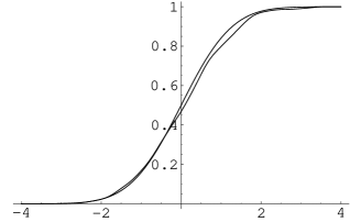
Figure 4: The final estimate $F_{nh}$ of $F$.

Figures 3 and 4 give the estimates $F^{-}_{nh}$, $F^{+}_{nh}$ and $F_{nh}$, based on the same sample of $n=500$ observations as above. Here the bandwidth use is $h=0.7$. Again, the original estimates are relatively accurate in one tail and almost periodic in the other tail. The combined estimate is accurate in both tails. Note the reduced variance in the tails of $F_{nh}$ compared to that of $F_{n}$ in Figure 2.

4 Proofs

4.1 Proof of Theorem 2.2

Note that

$$f^{-}_{nh}(x)=\sum_{j=0}^{\infty}g^{\prime}_{nh}(x-j)=\frac{1}{nh^{2}}\sum_{i=1}^{n}\sum_{j=0}^{\infty}w^{\prime}\Big{(}\frac{x-j-X_{i}}{h}\Big{)}$$

and

$$f^{{+}}_{nh}(x)=-\sum_{j=1}^{\infty}g^{\prime}_{nh}(x+j)=-\frac{1}{nh^{2}}\sum_{i=1}^{n}\sum_{j=1}^{\infty}w^{\prime}\Big{(}\frac{x+j-X_{i}}{h}\Big{)}.$$

Write

$$f^{(t)}_{nh}(x)=\sum_{i=1}^{n}\frac{1}{nh^{2}}\Big{(}t\sum_{j=0}^{\infty}w^{\prime}\Big{(}\frac{x-j-X_{i}}{h}\Big{)}-(1-t)\sum_{j=1}^{\infty}w^{\prime}\Big{(}\frac{x+j-X_{i}}{h}\Big{)}\Big{)}=\frac{1}{n}\sum_{i=1}^{n}U_{ih}(x)$$

where

$$U_{ih}(x)=\frac{1}{h^{2}}\Big{(}t\sum_{j=0}^{\infty}w^{\prime}\Big{(}\frac{x-j-X_{i}}{h}\Big{)}-(1-t)\sum_{j=1}^{\infty}w^{\prime}\Big{(}\frac{x+j-X_{i}}{h}\Big{)}\Big{)}.$$ (21)

First we compute the expectations of the estimators. By (6) we have

$${\rm E\,}f^{-}_{nh} (x)=\frac{1}{h^{2}}\sum_{j=0}^{\infty}{\rm E\,}w^{\prime}\Big{(}\frac{x-j-X_{1}}{h}\Big{)}=\frac{1}{h^{2}}\sum_{j=0}^{\infty}\int w^{\prime}\Big{(}\frac{x-j-u}{h}\Big{)}g(u)du$$

$$=\frac{1}{h}\sum_{j=0}^{\infty}\int w\Big{(}\frac{x-j-u}{h}\Big{)}g^{\prime}(u)du=\sum_{j=0}^{\infty}\frac{1}{h}\int w\Big{(}\frac{x-u}{h}\Big{)}g^{\prime}(u-j)du$$ (22)

$$=\frac{1}{h}\int w\Big{(}\frac{x-v}{h}\Big{)}f(v)dv$$

and similarly

$${\rm E\,}f^{+}_{nh}(x)=\frac{1}{h}\int w\Big{(}\frac{x-u}{h}\Big{)}f(u)du.$$ (23)

So the expectation of both $f^{-}_{nh}(x)$ and $f^{+}_{nh}(x)$ is equal to the expectation of an ordinary kernel estimator based on direct observations from $f$. From (22) and (23) we see that

$${\rm E\,}f^{(t)}_{nh}(x)=t{\rm E\,}f^{-}_{nh}(x)+(1-t){\rm E\,}f^{+}_{nh}(x)=\frac{1}{h}\int w\Big{(}\frac{x-u}{h}\Big{)}f(u)du.$$ (24)

The bias expansion in the theorem now follows by standard arguments.

Similar to (22) one can show ${\rm E\,}U_{1h}(x)=O(1)$ if $f$ is bounded on a neighborhood of $x$. The next lemma gives the even moments of $U_{ih}(x)$.

Lemma 4.1

For $m$ even we have for $h\to 0$

$${\rm E\,}U_{ih}(x)^{m}=\frac{1}{h^{2m-1}}(t^{m}F(x)+(-1)^{m}(1-t)^{m}(1-F(x))\int w^{\prime}(v)^{m}dv+O\Big{(}\frac{1}{h^{2m-2}}\Big{)}.$$ (25)

Proof

Note that

$$w^{\prime}\Big{(}\frac{x-j_{1}-X_{i}}{h}\Big{)}w^{\prime}\Big{(}\frac{x-j_{2}-X_{i}}{h}\Big{)}=0$$

if $j_{1}\not=j_{2},j_{1}\in\mathbb{Z},j_{2}\in\mathbb{Z}$ and $h<1/2$. Similarly it is readily seen that the products of terms $w^{\prime}\Big{(}\frac{x-j_{l}-X_{i}}{h}\Big{)}$ vanish if $h<1/2$ and if the $j_{l}$ are not all equal.

Now write

$${\rm E\,} U_{ih}(x)^{m}=\frac{1}{h^{2m}}{\rm E\,}\Big{(}t\sum_{j=0}^{\infty}w^{\prime}\Big{(}\frac{x-j-X_{i}}{h}\Big{)}-(1-t)\sum_{j=1}^{\infty}w^{\prime}\Big{(}\frac{x+j-X_{i}}{h}\Big{)}\Big{)}^{m}$$

$$=\frac{1}{h^{2m}}\Big{(}t^{m}\sum_{j=0}^{\infty}{\rm E\,}w^{\prime}\Big{(}\frac{x-j-X_{i}}{h}\Big{)}^{m}+(-1)^{m}(1-t)^{m}\sum_{j=1}^{\infty}{\rm E\,}w^{\prime}\Big{(}\frac{x+j-X_{i}}{h}\Big{)}^{m}\Big{)}$$

$$=\frac{1}{h^{2m-1}}\Big{(}t^{m}\sum_{j=0}^{\infty}\int w^{\prime}(v)^{m}g(x-j-hv)dv$$

$$\quad\quad+(-1)^{m}(1-t)^{m}\sum_{j=1}^{\infty}\int w^{\prime}(v)^{m}g(x+j-hv)dv\Big{)}$$

$$=\frac{1}{h^{2m-1}}\Big{(}t^{m}\int w^{\prime}(v)^{m}F(x-hv)dv$$

$$\quad\quad+(-1)^{m}(1-t)^{m}\int w^{\prime}(v)^{m}(1-F(x-hv))dv\Big{)}$$

$$=\frac{1}{h^{2m-1}}\,(t^{m}F(x)+(-1)^{m}(1-t)^{m}(1-F(x))\int w^{\prime}(v)^{m}dv+O\Big{(}\frac{1}{h^{2m-2}}\Big{)}.$$

$\Box$

For the variance of $f^{(t)}_{nh}(x)$ we get by Lemma 4.1

$$\mathop{\rm Var}\nolimits f^{(t)}_{nh} (x)=\frac{1}{n}\mathop{\rm Var}\nolimits(U_{1h}(x))=\frac{1}{n}\Big{(}{\rm E\,}U_{1h}(x)^{2}-({\rm E\,}U_{1h}(x))^{2}\Big{)}$$

$$\sim\frac{1}{nh^{3}}(t^{2}F(x)+(1-t)^{2}(1-F(x))\int w^{\prime}(v)^{2}dv.$$

We will now check the Lyapunov condition for $\frac{1}{n}\sum_{i=1}^{n}(U_{ih}(x)-{\rm E\,}U_{ih}(x))$ to be asymptotically normal, i.e. for some $\delta>0$ we have to check

$$\frac{{\rm E\,}|U_{1h}(x)-{\rm E\,}U_{1h}(x)|^{2+\delta}}{n^{\delta/2}(\mathop{\rm Var}\nolimits(U_{1h}(x)))^{1+\delta/2}}\to 0.$$

Using $(a+b)^{4}\leq 2^{3}(a^{4}+b^{4})$ we get, for suitable constants $c_{1}$ and $c_{2}$ to be obtained from Lemma 4.1,

$$\frac{{\rm E\,}(U_{1h}(x)-{\rm E\,}U_{1h}(x))^{4}}{n(\mathop{\rm Var}\nolimits(U_{1h}(x)))^{2}}\leq\frac{2^{3}({\rm E\,}U_{1h}(x)^{4}+({\rm E\,}U_{1h}(x))^{4})}{n(\mathop{\rm Var}\nolimits(U_{1h}(x)))^{2}}\sim\frac{8c_{1}}{nhc_{2}^{2}}\to 0.$$

This proves asymptotic normality of $(f^{(t)}_{nh}(x)-{\rm E\,}f^{(t)}_{nh}(x))/\sqrt{\mathop{\rm Var}\nolimits f^{(t)}_{nh}(x)}$ for fixed $t$. $\Box$

4.2 Proof of Theorem 2.3

We must show that we can replace $t=1-F(x)$ by a consistent estimator. Write

$$f_{nh}(x)=(1-\hat{F}_{n}(x))f^{-}_{nh}(x)+\hat{F}_{n}(x)f^{+}_{nh}(x)=f_{nh}^{(1-F(x))}(x)+R_{nh}(x),$$ (26)

where

$$R_{nh}(x)=(\hat{F}_{n}(x)-F(x))S_{nh}(x)\quad\mbox{and}\quad S_{nh}(x)=f^{+}_{nh}(x)-f^{-}_{nh}(x).$$ (27)

Now write

$$S_{nh}(x)=\frac{1}{n}\sum_{i=1}^{n}W_{ih}(x),$$

where

$$W_{ih}(x)=\frac{1}{h^{2}}\sum_{j=-\infty}^{\infty}w^{\prime}\Big{(}\frac{x-j-X_{i}}{h}\Big{)}.$$

The next lemma establishes some properties of $S_{nh}(x)$.

Lemma 4.2

We have ${\rm E\,}S_{nh}(x)=0$, ${\rm E\,}W_{ih}(x)^{m}=\frac{1}{h^{2m-1}}\int w^{\prime}(u)^{m}du$ and

$$\sqrt{nh^{3}}S_{nh}(x)\stackrel{{\scriptstyle\cal D}}{{\rightarrow}}N\Big{(}0,\int w^{\prime}(u)^{2}du\Big{)}.$$

The distributions of the random variables $W_{ih}(x)$ and $S_{nh}(x)$ are independent of $x$.

Proof

The first statement follows from (22) and (23). The second statement follows from a computation similar to the one in the proof of Lemma 4.1. Asymptotic normality can be proved as in the proof of Theorem 2.2.

The fact that the distribution does not depend on $x$ can be seen by writing

$$\sum_{j=-\infty}^{\infty}w^{\prime}\Big{(}\frac{x-j-X_{i}}{h}\Big{)}=\sum_{j=-\infty}^{\infty}w^{\prime}\Big{(}\frac{x-j-Y_{i}-Z_{i}}{h}\Big{)}.$$

Given $x$ and $Y_{i}$ this sum equals a periodic function with period one evaluated at $Z_{i}$. Since $Z_{i}$ is Uniform$[0,1)$ distributed its distribution does not depend on $x$ and $Y_{1}$.

$\Box$

By (10) we have $\hat{F}_{n}(x)-F(x)\stackrel{{\scriptstyle P}}{{\rightarrow}}0$ and hence by Slutsky’s theorem $\sqrt{nh^{3}}R_{nh}(x)\stackrel{{\scriptstyle P}}{{\rightarrow}}0.$ Furthermore by the Cauchy-Schwarz inequality

$${\rm E\,}\sqrt{nh^{3}}|R_{nh}(x)|\leq\sqrt{nh^{3}}({\rm E\,}(\hat{F}_{n}(x)-F(x))^{2})^{1/2}({\rm E\,}(S_{nh}(x))^{2})^{1/2}\to 0.$$

This shows that $\sqrt{nh^{3}}(f_{nh}(x)-{\rm E\,}f_{nh}(x))$ has the same asymptotic normal distribution as $\sqrt{nh^{3}}(f_{nh}^{(1-F(x))}(x)-{\rm E\,}f_{nh}^{(1-F(x))}(x))$, which proves the first statement of the theorem.

To prove the second statement note that by (24) and a standard argument in kernel estimation we have

$${\rm E\,}f_{nh}^{(1-F(x))}(x)=\frac{1}{h}\int w\Big{(}\frac{x-u}{h}\Big{)}f(u)du=f(x)+\frac{1}{2}h^{2}f^{\prime\prime}(x)\int v^{2}w(v)dv+o(h^{2}).$$ (28)

Furthermore

$${\rm E\,}|R_{nh}(x)| \leq({\rm E\,}(\hat{F}_{n}(x)-F(x))^{2})^{1/2}({\rm E\,}(S_{nh}(x))^{2})^{1/2}$$

$$=o\Big{(}\sqrt{nh^{7}}\Big{)}O\Big{(}\frac{1}{\sqrt{nh^{3}}}\Big{)}=o(h^{2}).$$ (29)

Together (28) and (29) prove the second statement of the theorem. $\Box$

4.3 Proof of Theorem 2.6

We copy the proof of Theorem 2.3. Note that

$$F^{-}_{nh}(x)=\sum_{j=0}^{\infty}g_{nh}(x-j)=\frac{1}{nh}\sum_{i=1}^{n}\sum_{j=0}^{\infty}w\Big{(}\frac{x-j-X_{i}}{h}\Big{)}$$

and

$$F^{+}_{nh}(x)=1-\sum_{j=1}^{\infty}g_{nh}(x+j)=1-\frac{1}{nh}\sum_{i=1}^{n}\sum_{j=1}^{\infty}w\Big{(}\frac{x+j-X_{i}}{h}\Big{)}.$$

Write

$$F^{(t)}_{nh} (x)=tF^{-}_{nh}(x)+(1-t)F^{+}_{nh}(x)$$

$$=\sum_{i=1}^{n}\frac{1}{nh}\Big{(}t\sum_{j=0}^{\infty}w\Big{(}\frac{x-j-X_{i}}{h}\Big{)}-(1-t)\sum_{j=1}^{\infty}w\Big{(}\frac{x+j-X_{i}}{h}\Big{)}\Big{)}+1-t$$

$$=\frac{1}{n}\sum_{i=1}^{n}V_{ih}(x)+1-t$$

where

$$V_{ih}(x)=\frac{1}{h}\Big{(}t\sum_{j=0}^{\infty}w\Big{(}\frac{x-j-X_{i}}{h}\Big{)}-(1-t)\sum_{j=1}^{\infty}w\Big{(}\frac{x+j-X_{i}}{h}\Big{)}\Big{)}.$$

First we compute the expectations of the estimators. By (6) we have

$${\rm E\,}F^{-}_{nh} (x)=\frac{1}{h}\sum_{j=0}^{\infty}{\rm E\,}w\Big{(}\frac{x-j-X_{1}}{h}\Big{)}=\frac{1}{h}\sum_{j=0}^{\infty}\int w\Big{(}\frac{x-j-u}{h}\Big{)}g(u)du$$

$$=\sum_{j=0}^{\infty}\frac{1}{h}\int w\Big{(}\frac{x-u}{h}\Big{)}g(u-j)du$$ (30)

$$=\frac{1}{h}\int w\Big{(}\frac{x-u}{h}\Big{)}F(u)du$$

and similarly

$${\rm E\,}F^{+}_{nh}(x)=\frac{1}{h}\int w\Big{(}\frac{x-u}{h}\Big{)}F(u)du.$$ (31)

Since it is a convex combination of $F^{-}_{nh}(x)$ and $F^{+}_{nh}(x)$ the expectation of $F^{(t)}_{nh}(x)$ is also equal to (30) and (31).

The equivalent to Lemma 4.1 for $V_{ih}(x)$ is

$${\rm E\,}V_{ih}(x)^{m}=\frac{1}{h^{m-1}}(t^{m}F(x)+(-1)^{m}(1-t)^{m}(1-F(x))\int w(v)^{m}dv+o\Big{(}\frac{1}{h^{m-1}}\Big{)}$$ (32)

which follows by replacing $w^{\prime}$ by $w$ and replacing $1/h^{2}$ by $1/h$ in the proof.

For the variance of $F^{(t)}_{nh}(x)$ we then get

$$\mathop{\rm Var}\nolimits F^{(t)}_{nh} (x)=\frac{1}{n}\mathop{\rm Var}\nolimits(V_{1h}(x))=\frac{1}{n}\Big{(}{\rm E\,}V_{1h}(x)^{2}-({\rm E\,}V_{1h}(x))^{2}\Big{)}$$

$$\sim\frac{1}{nh}(t^{2}F(x)+(1-t)^{2}(1-F(x))\int w(v)^{2}dv.$$

The Lyapunov condition for $\frac{1}{n}\sum_{i=1}^{n}(V_{ih}(x)-{\rm E\,}V_{ih}(x))$ to be asymptotically normal can be checked as in the proof of Theorem 2.3. This proves asymptotic normality of $(F^{(t)}_{nh}(x)-{\rm E\,}F^{(t)}_{nh}(x))/\sqrt{\mathop{\rm Var}\nolimits F^{(t)}_{nh}(x)}$ for fixed $t$. $\Box$

4.4 Proof of Theorem 2.8

Recall that by (26) we have

$$f_{nh}(x)=f_{nh}^{(1-F(x))}(x)+R_{nh}(x),$$

where

$$R_{nh}(x)=(\hat{F}_{n}(x)-F(x))S_{nh}(x)\quad\mbox{and}\quad S_{nh}(x)=f^{+}_{nh}(x)-f^{-}_{nh}(x).$$

We decompose the mean integrated squared error as follows

$${\rm MISE_{n}} (h)=\int{\rm E\,}\Big{(}f_{nh}^{(1-F(x))}(x)-f(x)+R_{nh}(x)\Big{)}^{2}dx$$

$$=\int{\rm E\,}\Big{(}f_{nh}^{(1-F(x))}(x)-f(x)\Big{)}^{2}dx+\int{\rm E\,}R_{nh}(x)^{2}dx$$ (33)

$$\quad\quad+2\int{\rm E\,}\Big{(}(f_{nh}^{(1-F(x))}(x)-f(x)\Big{)}R_{nh}(x))dx.$$ (34)

The mean integrated squared error of $f_{nh}^{(1-F(x))}$ can be written as integrated squared bias plus integrated squared variance. We have

$$\int{\rm E\,}(f_{nh}^{(1-F(x))}(x)-f(x))^{2}dx=\int({\rm E\,}f_{nh}^{(1-F(x))}(x)-f(x))^{2}dx+\int\mathop{\rm Var}\nolimits f_{nh}^{(1-F(x))}(x)dx.$$

We have already noted in (24) that the expectation of $f_{nh}^{(1-F(x))}(x)$ is equal to the expectation of a standard kernel estimator. By Theorem 2.1.7 of Prakasa Rao (1983), or the original proof of Nadaraya, we have the standard expansion for integrated squared bias of $f_{nh}^{(1-F(x))}(x)$, i.e.

$$\int({\rm E\,}f_{nh}^{(1-F(x))}(x)-f(x))^{2}dx=\frac{1}{4}h^{4}\int f^{\prime\prime}(x)^{2}dx\Big{(}\int v^{2}w(v)dv\Big{)}^{2}+o(h^{4}).$$

Next consider the integrated variance. We have, with $U_{ih}(x)$ as in (21),

$$\mathop{\rm Var}\nolimits f_{nh}^{(1-F(x))}(x)=\frac{1}{n}\mathop{\rm Var}\nolimits(U_{1h}(x))=\frac{1}{n}\Big{(}{\rm E\,}U_{1h}(x)^{2}-({\rm E\,}U_{1h}(x))^{2}\Big{)},$$ (35)

where by the proof of Lemma 4.1, with $t=1-F(x)$,

$${\rm E\,}U_{1h}(x)^{m}=\frac{1}{h^{2m-1}}\Big{(}(1-F(x))^{m}\int w^{\prime}(v)^{m}F(x-hv)dv+(-1)^{m}F(x)^{m}\int w^{\prime}(v)^{m}(1-F(x-hv))dv\Big{)}$$

Now use

$$F(x-hv)=F(x)-hv\int_{0}^{1}f(x-thv)dt$$

to get

$${\rm E\,}U_{1h}(x)^{2}= \frac{1}{h^{3}}F(x)(1-F(x))\int w^{\prime}(v)^{2}dv$$

$$-\frac{1}{h^{2}} ((1-F(x))^{2}+F(x)^{2})\int_{-1}^{1}\int_{0}^{1}vw^{\prime}(v)^{2}f(x-thv)dvdt.$$

The integral with respect to $x$ of the first term is finite by the condition ${\rm E\,}Y<\infty$. The integral with respect to $x$ of the second term is finite by the fact that $|(1-F(x))^{2}+F(x)^{2}|$ is bounded by two and Fubini’s theorem. Similarly, for the term ${\rm E\,}U_{1h}(x)$ in (35) we get by the Cauchy Schwartz inequality and Fubini’s theorem

$$\int({\rm E\,}U_{1h}(x))^{2} dx=\int\Big{(}\int_{-1}^{1}\int_{0}^{1}vw^{\prime}(v)f(x-thv)dvdt\Big{)}^{2}dx$$

$$\leq\int\Big{(}\int_{-1}^{1}\int_{0}^{1}v^{2}w^{\prime}(v)^{2}dvdt\int_{-1}^{1}\int_{0}^{1}f(x-thv)^{2}dvdt\Big{)}dx$$

$$=\int_{-1}^{1}\int_{0}^{1}v^{2}w^{\prime}(v)^{2}dvdt\int\int_{-1}^{1}\int_{0}^{1}f(x-thv)^{2}dxdvdt$$

$$=2\int_{-1}^{1}v^{2}w^{\prime}(v)^{2}dv\int f(x)^{2}dx.$$

Finally this gives

$$\int\mathop{\rm Var}\nolimits f_{nh}^{(1-F(x))}(x)dx=\frac{1}{nh^{3}}F(x)(1-F(x))\int w^{\prime}(v)^{2}dv+O\Big{(}\frac{1}{nh^{2}}\Big{)}.$$

For the integrated expected squared remainder term in (33) we have

$$\int{\rm E\,}R_{nh} (x)^{2}dx=\int{\rm E\,}(\hat{F}_{n}(x)-F(x))^{2}S_{nh}(x)^{2}dx$$

$$\leq\int({\rm E\,}(\hat{F}_{n}(x)-F(x))^{4})^{1/2}({\rm E\,}S_{nh}(x)^{4})^{1/2}dx$$

$$=o(nh^{7})O\Big{(}\frac{1}{nh^{3}}\Big{)}=o(h^{4}),$$

since by Lemma 4.2

$$({\rm E\,}S_{nh}(x)^{4} )^{1/2}=\Big{\{}\frac{1}{n^{4}}\Big{[}n{\rm E\,}W_{1h}(x)^{4}+3n(n-1)({\rm E\,}W_{1h}(x))^{2}\Big{]}\Big{\}}^{1/2}$$

$$=\Big{\{}\frac{1}{n^{4}}\Big{[}n\Big{(}\frac{1}{h^{7}}\int w^{\prime}(v)^{4}dv\Big{)}+3n(n-1)\Big{(}\frac{1}{h^{3}}\int w^{\prime}(v)^{2}dv\Big{)}^{2}\Big{]}\Big{\}}^{1/2}=O\Big{(}\frac{1}{nh^{3}}\Big{)}.$$

The proof of the theorem is completed by noting that the cross product term (34) is negligible with respect to the first term (33) by the Cauchy Schwartz inequality. $\Box$

4.5 Proof of Lemma 2.9

Write

$$F_{nh}^{(H(x))}(x)-F(x)=F_{nh}^{(H(x))}(x)-{\rm E\,}F_{nh}^{(H(x))}(x)+{\rm E\,}F_{nh}^{(H(x))}(x)-F(x)$$

By the triangle inequality we have

$$\Big{(}{\rm E\,}(F_{nh}^{(H(x))}(x)-F(x))^{4}\Big{)}^{1/4}\leq\Big{(}{\rm E\,}(F_{nh}^{(H(x))}(x)-{\rm E\,}F_{nh}^{(H(x))}(x))^{4}\Big{)}^{1/4}+\Big{(}{\rm E\,}F_{nh}^{(H(x))}(x)-F(x)\Big{)}.$$

So by $(a+b)^{2}\leq 2(a^{2}+b^{2}),a,b\geq 0$, we also have

$$\Big{(}{\rm E\,}(F_{nh}^{(H(x))}(x)-F(x))^{4}\Big{)}^{1/2}\leq 2\Big{(}{\rm E\,}(F_{nh}^{(H(x))}(x)-{\rm E\,}F_{nh}^{(H(x))}(x))^{4}\Big{)}^{1/2}+2\Big{(}{\rm E\,}F_{nh}^{(H(x))}(x)-F(x))\Big{)}^{2}.$$

Hence it suffices to prove the bound of the lemma for the fourth power of the error and the usual square of the bias separately.

In the proof of Theorem 2.6 we have seen that $F_{nh}^{(H(x))}(x)$ can be written as

$$F^{(H(x))}_{nh}(x)=\frac{1}{n}\sum_{i=1}^{n}V_{ih}(x)+H(x)$$

where

$$V_{ih}(x)=\frac{1}{h}\Big{(}(1-H(x))\sum_{j=0}^{\infty}w\Big{(}\frac{x-j-X_{i}}{h}\Big{)}-H(x)\sum_{j=1}^{\infty}w\Big{(}\frac{x+j-X_{i}}{h}\Big{)}\Big{)}.$$

and that we have

$${\rm E\,}F^{(H(x))}_{nh}(x)=\frac{1}{h}\int w\Big{(}\frac{x-u}{h}\Big{)}F(u)du.$$

Following the same arguments as in the proof of Theorem 2.1.7, the MISE expansion for kernel estimators, of Prakasa Rao (1983) we have

$$\int_{-\infty}^{\infty}({\rm E\,}F_{nh}^{(H(x))}(x)-F(x))^{2}dx=\frac{1}{4}h^{4}\Big{(}\int_{-\infty}^{\infty}f^{\prime}(x)^{2}dx\Big{)}\Big{(}\int_{-\infty}^{\infty}v^{2}w(v)dv\Big{)}^{2}+o(h^{4}).$$ (36)

In order to deal with the error part we wite

$$F^{(H(x))}_{nh}(x)-{\rm E\,}F^{(H(x))}_{nh}(x)=\frac{1}{n}\sum_{i=1}^{n}\tilde{V}_{ih}(x),$$

where $\tilde{V}_{ih}(x)=V_{ih}(x)-{\rm E\,}V_{ih}(x)$. Since ${\rm E\,}\tilde{V}_{ih}(x)$ equals zero we have

$${\rm E\,}\Big{(}\frac{1}{n}\sum_{i=1}^{n}\tilde{V}_{ih}(x)\Big{)}^{4}=\frac{1}{n^{3}}{\rm E\,}\Big{(}\tilde{V}_{1h}(x)^{4}\Big{)}+3\,\frac{n-1}{n^{3}}\Big{(}{\rm E\,}\Big{(}\tilde{V}_{1h}(x)^{2}\Big{)}\Big{)}^{2}.$$

From (32) we get

$$\frac{1}{n^{3}}{\rm E\,}\Big{(}\tilde{V}_{1h}(x)^{4}\Big{)}\sim\frac{1}{n^{3}}{\rm E\,}\Big{(}V_{1h}(x)^{4}\Big{)}\sim\frac{c_{1}}{n^{3}h^{3}}\,\Big{(}(1-H(x))^{4}F(x)+H(x)^{4}(1-F(x))\Big{)}$$

and

$$3\,\frac{n-1}{n^{3}}\Big{(}{\rm E\,}\Big{(}\tilde{V}_{1h}(x)^{2}\Big{)}\Big{)}^{2}=3\,\frac{n-1}{n^{3}}\big{(}\mathop{\rm Var}\nolimits(V_{1h}(x))^{2}\Big{)}\sim\frac{c_{2}}{n^{2}h^{2}}\,\Big{(}(1-H(x))^{2}F(x)+H(x)^{2}(1-F(x))\Big{)}^{2},$$

for certain constants $c_{1}$ and $c_{2}$. Since the square roots of the functions on the right hand side are integrable we now have

$$\int_{\infty}^{\infty}\Big{(}{\rm E\,}(F^{(H(x))}_{nh}(x)-{\rm E\,}F^{(H(x))}_{nh}(x))^{4}\Big{)}^{1/2}dx=O\Big{(}\frac{1}{nh}\Big{)}$$

Summarizing we get

$$\int_{\infty}^{\infty}\Big{(}{\rm E\,}(F_{nh}^{(H(x))}(x)-F(x))^{4}\Big{)}^{1/2}dx=O(h^{4})+O\Big{(}\frac{1}{nh}\Big{)},$$

which completes the proof. $\Box$

5 The limit variance of the smoothed NPMLE

In this section we will show that the limit variance of the smoothed NPMLE is equal to the limit variance of our optimally combined kernel estimator.

Let the distribution induced by $F$ have support $[0,M)$ for some $M>0$ and let $m$ denote the largest integer strictly smaller than $M+1$. The asymptotic variance of the smoothed NPMLE in Theorem 2 in Groeneboom and Jongbloed (2003) is, in their notation where $t$ stands for our $x$ in Theorem 2.3, defined as

$$\sigma^{2}=\lim_{h\downarrow 0}\int\theta^{2}_{h,t,F}dG,$$ (37)

with the function $\theta_{h,t,F}$, for $0\leq t<M$, defined by

$$\theta_{h,t,F}(x+k)=\left\{\begin{array}[]{ll}\sum_{i=0}^{m}(1-F(x+i))w_{h}^{\prime}(t-(x+i))&,\ \mbox{if}\ x\in[0,1],\ k=0,\\ -\sum_{i=0}^{k-1}w_{h}^{\prime}(t-(x+i))+\theta_{h,t,F}(x)&,\ \mbox{if}\ x\in[0,1],\ k=1,\ldots,m,\end{array}\right.$$ (38)

where $w_{h}(\cdot)=w(\cdot/h)/h$.

Lemma 5.1

The asymptotic variance (37) is equal to $F(t)(1-F(t))\int w^{\prime}(u)^{2}du.$

Proof We write the integral in (37) as

$$\int \theta^{2}_{h,t,F}dG=\sum_{k=0}^{m}\int_{0}^{1}\theta^{2}_{h,t,F}(x+k)g(x+k)dx$$

$$=\int_{0}^{1}(F(x)-F(x-1))\Big{[}(1-F(x))w_{h}^{\prime}(t-x)+(1-F(x+1))w_{h}^{\prime}(t-x-1)$$

$$\quad\quad+(1-F(x+2))w_{h}^{\prime}(t-x-2)+\ldots+(1-F(x+m))w_{h}^{\prime}(t-x-m)\big{]}^{2}dx$$

$$+\int_{0}^{1}(F(x+1)-F(x))\Big{[}-F(x)w_{h}^{\prime}(t-x)+(1-F(x+1))w_{h}^{\prime}(t-x-1)$$

$$\quad\quad+(1-F(x+2))w_{h}^{\prime}(t-x-2)+\ldots+(1-F(x+m))w_{h}^{\prime}(t-x-m)\big{]}^{2}dx$$

$$+\int_{0}^{1}(F(x+2)-F(x+1))\Big{[}-F(x)w_{h}^{\prime}(t-x)-F(x+1)w_{h}^{\prime}(t-x-1)$$

$$\quad\quad+(1-F(x+2))w_{h}^{\prime}(t-x-2)+\ldots+(1-F(x+m))w_{h}^{\prime}(t-x-m)\big{]}^{2}dx$$

$$+\ldots$$

$$+\int_{0}^{1}(F(x+m)-F(x+m-1))\Big{[}-F(x)w_{h}^{\prime}(t-x)-F(x+1)w_{h}^{\prime}(t-x-1)$$

$$\quad\quad-F(x+2)w_{h}^{\prime}(t-x-2)+\ldots-F(x+m)w_{h}^{\prime}(t-x-m)\Big{]}^{2}dx.$$

The next step is to write out the squares, which we leave to the reader. Let $l\leq t<l+1$ for some integer $l$, then, since $0\leq t-l<1$ and $x\in[0,1]$, only the terms containing $w_{h}^{\prime}(t-x-l)^{2}$ will yield a non zero contribution for $h$ small enough. This contribution is, for $h$ to zero, equal to

$$\int_{0}^{1}\sum_{j=0}^{l}(F(x+j)-F(x+j-1))(1-F(x+l))^{2}w_{h}^{\prime}(t-x-l)^{2}dx$$

$$\quad\quad+\int_{0}^{1}\sum_{j=l+1}^{m}(F(x+j)-F(x+j-1))F(x+l)^{2}w_{h}^{\prime}(t-x-l)^{2}dx$$

$$=\int_{0}^{1}F(x+l)(1-F(x+l))^{2}w_{h}^{\prime}(t-x-l)^{2}dx$$

$$\quad\quad+\int_{0}^{1}(1-F(x+l))F(x+l)^{2}w_{h}^{\prime}(t-x-l)^{2}dx$$

$$\sim\frac{1}{h^{3}}\,\Big{(}F(t)(1-F(t))^{2}+(1-F(t))F(t)^{2}\Big{)}\int w^{\prime}(u)^{2}du$$

$$=\frac{1}{h^{3}}\,F(t)(1-F(t))\int w^{\prime}(u)^{2}du.$$

Here we have used an expansion of the integral which is standard in kernel estimation theory.

Taking the limit for $h$ to zero as in (37) now yields the result. $\Box$

References

- [1] S. Donauer. Asymptotics in Deconvolution Models - Approximating Perfect Knowledge. PhD. thesis Delft University of Technology, 2009.
- [2] A.J. van Es. Uniform deconvolution: Nonparametric maximum likelihood and inverse estimation. In: Nonparametric Functional Estimation and Related Topics, (G. Roussas ed.). Kluwer Academic Publishers, Dordrecht, 191–198, 1991.
- [3] A.J. van Es and A.R. Kok. Simple kernel estimators for certain nonparametric deconvolution problems. Statist. Probab. Lett., 39:151–160, 1998.
- [4] A.J. van Es and M.C.A. van Zuijlen. Convex minorant estimators in nonparametric deconvolution problems. Scand. J. Statist. 23: 85–104, 1996.
- [5] J. Fan. Adaptively local one-dimensional subproblems with application to a deconvolution problem. Ann. Statist. 21: 600–610, 1993.
- [6] A. Feuerverger, P.T. Kim and J. Sun. On optimal uniform deconvolution. J. Stat. Theory Pract. 3: 433–451, 2008.
- [7] P. Groeneboom and G. Jongbloed. Density estimation in the uniform deconvolution model. Statist. Neerlandica 57: 136–157, 2003.
- [8] P. Groeneboom and J.A. Wellner. Information Bounds and Nonparametric Maximum Likelihood. Birkhäuser, Basel, 1992.
- [9] P. Hall and A. Meister. A ridge-parameter approach to deconvolution. Ann. Statist., 35: 1535–1558, 2007.
- [10] Y. Hu and G. Ridder. Estimation of nonlinear models with measurement error using marginal information. Econometric Society North American Summer Meetings 21, Econometric Society. available at http://ideas.repec.org/p/ecm/nasm04/21.html, 2004.
- [11] G. Jongbloed. Exponential deconvolution: two asymptotically equivalent estimators. Statist. Neerlandica 52: 6–17, 1998.
- [12] B.L.S. Prakasa Rao. Nonparametric Functional Estimation. Academic Press, New York, 1983.
- [13] B.W. Silverman. Density Estimation for Statistics and Data Analysis. Chapman and Hall, London, 1986.
- [14] M.P. Wand and M.C. Jones. Kernel Smoothing. Chapman and Hall, London, 1995.