The degree distribution in bipartite planar maps: applications to the Ising model

Abstract

We characterize the generating function of bipartite planar maps counted according to the degree distribution of their black and white vertices. This result is applied to the solution of the hard particle and Ising models on random planar lattices. We thus recover and extend some results previously obtained by means of matrix integrals.

Proofs are purely combinatorial and rely on the idea that planar maps are conjugacy classes of trees. In particular, these trees explain why the solutions of the Ising and hard particle models on maps of bounded degree are always algebraic.

1 Introduction

The enumeration of planar maps (i.e., connected graphs drawn on the sphere with non-intersecting edges) has received a lot of attention since the 60’s. Four decades of exploration have resulted into three main enumeration techniques, and two types of results: first, a few remarkable families of maps are counted by very nice and simple numbers; second, and more generally, many families of maps share the characteristic of having an algebraic generating function. Meanwhile, many exciting connections have been established between maps and various branches of mathematics, like Grothendieck’s theory of "dessins d’enfants" or knot theory, and, most importantly for this paper, between maps and certain branches of physics.

This paper presents a combinatorial approach for solving two types of physics models on maps: the Ising and hard particle models. In these models, the vertices of the maps carry spins or particles; their solution is equivalent to a weighted enumeration of maps. The weight is in general a specialization of the Tutte polynomial of the map.

The idea of putting such a model on maps originates in physics, and more precisely in two-dimensional quantum gravity: in this theory, maps arise as discrete models of geometries, or random planar lattices, and a lattice not carrying any spin or particle is only moderately interesting. As can be observed in numerous occasions, physicists are not only good at doing physics: in this case, Br zin et al., in the steps of t’Hooft [24], developed a new approach for counting maps, completely different from what had been done previously in combinatorics. This approach, suggested by quantum field theory, is based on the evaluation of matrix integrals with well chosen potentials [3, 8]. An introduction to these techniques, intended for mathematicians, is presented in [29], and a far reaching account can be found in [12].

This approach is extremely powerful: it allows to produce quickly expressions for generating functions without requiring much invention at the combinatorial level. In particular, the Ising model on tri- and on tetravalent maps (maps with vertices of degree 3 or 4) was solved via this approach in the late 80’s, yielding intriguing algebraic generating functions [4, 17, 19]; the same kind of technique was applied much more recently to the hard particle model on a larger variety of maps [6]. However, the evaluation of the matrix integrals as presented in most papers is not satisfying from the mathematical point of view: justifications of the calculations are often omitted, whereas they involve non-trivial complex analysis and resummation issues. Moreover, this approach gives little insight on the combinatorial structure of maps and does not explain the algebraic nature of the generating functions thus obtained.

The material presented in this paper provides an alternative approach to the Ising and hard particle models, and has none of the above mentioned drawbacks. It is essentially of a bijective nature, and only involves elementary combinatorial arguments. We show that certain families of plane trees are at the heart of both models, and this justifies the algebraicity of their solutions. We do not study the singularities of the series we obtain, even though they are very significant from the physics point of view: this has already been done in [4, 6, 17], and is anyway routine for algebraic series.

The central objects of our paper are actually the bipartite maps, which we enumerate according to the degree distribution of their black and white vertices. We thus extend the results of [5] on the so-called constellations, and also the results of [7] on the degree distribution of (unicolored) planar maps (the latter being in one-to-one correspondence with bipartite maps in which all black vertices have degree two). Then, we show that the solutions of the Ising and hard particle models are closely related to the enumeration of bipartite maps.

Our approach provides a new illustration of the principle according to which planar maps are, in essence, conjugacy classes of trees. This idea was introduced by the second author of this paper in order to explain bijectively certain nice formulae for the number of maps [22, 23]. Then, it led to a common generalization of formulae of Tutte and Hurwitz [5], before being adapted to maps satisfying 2- and 3-connectivity constraints [20, 21]. A few months ago, Bouttier et al. cleverly built on the same idea to give a bijective derivation of Bender and Canfield’s solution of the very general problem of counting maps by the degree distribution of their vertices [2, 7].

Let us mention that the seminal work of Tutte on the enumeration of maps was not based on bijections, but on recursive decompositions of maps, which led to functional equations for their generating functions. This type of approach is usually fairly systematic; combined with the so-called quadratic method and its generalizations, it has provided many algebraicity results, including recent ones [2, 9, 14, 25, 26]. It yields short self-contained proofs, relying only on elementary decompositions and algebraic calculus in the realm of formal power series. However, as far as we know, there has been very few successful attempts to apply this method to the enumeration of maps carrying an additional structure, like an Ising model. Roughly speaking, the standard decompositions of maps still provide certain functional equations, but these are much harder to solve that in the previous cases. This is perfectly illustrated by the tour de force achieved by Tutte, who spent 10 years solving the equation he had established for the chromatic polynomial of triangulations [27].

For the sake of completeness, let us mention a few additional results and techniques. The first bijective proofs in map enumeration are due to Cori [10] and later to Arqu s [1]. Some models involving self-avoiding walks on maps can essentially be solved without matrix integrals [13], by using enumeration results due to Tutte. Then, a cluster expansion method has been developed very recently for a general model of spins with neighbor interactions on maps [18]. However, this provides only partial qualitative results and does not allow to recover the critical exponents of the hard particle and Ising models (whereas they can be derived from the generating functions obtained either with our approach or with matrix integrals). Finally, the enumerative theory of ramified coverings of the sphere has led a number of authors to consider a very refined enumeration of maps on higher genus surfaces, in which the degrees of vertices and faces are taken into account. The relevant methods rely on the encoding of maps by permutations [11] and lead to expressions involving characters of the symmetric group [15, 16]. However, to the best of our knowledge, none of the simple generating functions of planar maps have ever been rederived from these expressions.

2 A glimpse at the results

To begin with, let us recall a few definitions and conventions. A planar map is a 2-cell decomposition of the oriented sphere into vertices (0-cells), edges (1-cells) and faces (2-cells). In more vernacular terms, it is a connected graph drawn on a sphere with non-intersecting edges. Loops and multiple edges are allowed. Two maps are isomorphic if there exists an orientation preserving homeomorphism of the sphere that sends one onto the other. A map is rooted if one of its edges is distinguished and oriented. In this case, the map is drawn on the plane in such a way the infinite face lies to the right of the root edge. All the maps considered in this paper are planar, rooted, and considered up to isomorphisms. An example is provided in Figure 1.1; this map is tetravalent, meaning that all vertices have degree $4$. In the physics literature, authors often consider unrooted maps; but they count them with a symmetry factor which makes the problem equivalent to counting rooted maps, up to a differentiation of the (unrooted) generating function.

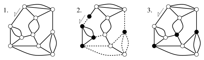
Figure 1: 1. A tetravalent map – 2. An Ising configuration on a quasi-tetravalent map with 8 frustrated edges (dashed edges) – 3. A hard particle configuration with 3 particles on a tetravalent map.

In combinatorial terms, the solution of the Ising model on planar maps (in a magnetic field) is equivalent to counting maps having vertices of two types (white and black): one has to count them, not only by their number of edges and vertices of each color, but also by the number of frustrated edges, that is, edges that are adjacent to a white vertex and to a black one.

The tools developed in this paper allow us to solve the Ising model on any class of maps subject to degree conditions. The associated generating functions are algebraic as soon as the degrees of the vertices are bounded. Here is, for instance, the result we obtain for “quasi-tetravalent” maps: maps having only vertices of degree $4$, except for the root vertex which has degree $2$ (Figure 1.2).

Proposition 1 (Ising on quasi-tetravalent maps)

Let $I(X,Y,u)$ be the generating function for bicolored quasi-tetravalent maps, rooted at a black vertex, where the variable $X$ (resp. $Y$) counts the number of white (resp. black) vertices of degree $4$, and $u$ counts the number of frustrated edges. Let $P(x,y,v)\equiv P$ be the power series defined by the following algebraic equation:

$$P=1+3xyP^{3}+v^{2}\ \frac{P(1+3xP)(1+3yP)}{(1-9xyP^{2})^{2}}.$$

Then the Ising generating function $I(X,Y,u)$ can be expressed in terms of $P(x,y,v)$, with $x=X(u-\bar{u})^{2},y=Y(u-\bar{u})^{2}$, and $v=\bar{u}=1/u$. One possible expression is:

$$\frac{I(X,Y,u)}{1-\bar{u}^{2}}=xP^{3}+\frac{P(1+3xP-2xP^{2}-6xyP^{3})}{1-9xyP^{2}}-\frac{yv^{2}P^{3}(1+3xP)^{3}}{(1-9xyP^{2})^{3}}.$$

As $P$ itself, the series $I(X,Y,u)$ is algebraic of degree $7$.

Remarks
1. Replacing $X$ by $tX$ and $Y$ by $tY$ gives a generating function in which tetravalent vertices are counted by $t$. The expansion of the Ising generating function then begins as follows:

$$I(tX,tY,u)=1+t(2Xu^{2}+2Y)+t^{2}\left(9X^{2}u^{2}+9Y^{2}+XY(12u^{2}+6u^{4})\right)+O(t^{3}).$$

These terms correspond to maps having at most two tetravalent vertices; they are shown on Figure 2.
2. It is easy to check that the parametrization by $P$ is equivalent to the one given by Boulatov and Kazakov for the free energy of the Ising model on tetravalent maps [4, Eq. (17)].

Proposition 1 will only be proved in Section 7. At the heart of the proof is the fact that the series $P$ is the generating function of certain trees, as suggested by the equation defining $P$. We shall also prove that the Ising generating function for truly tetravalent maps belongs to the same algebraic extension of $\mathbb{Q}[X,Y,u]$ as $P$. But its expression in terms of $P$ is messier (Proposition 22).

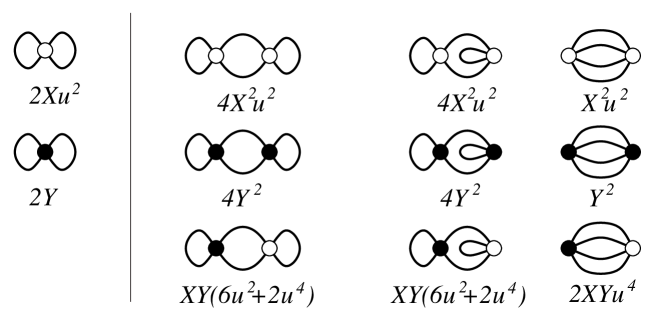
Figure 2: The (unrooted) tetravalent maps having a most two vertices. The polynomials in $X,Y$ and $u$ describe the number of ways of adding a black root vertex of degree $2$ and the Ising weight of the resulting quasi-tetravalent maps.

Observe that the series $I(X,Y,u)$ contains all the information we need to count also the number of uniform (non-frustrated) edges. In particular, the series $uI(X,Yu^{2},1/\sqrt{u})$ counts bicolored quasi-tetravalent maps by their white and black vertices (variables $X$ and $Y$), and by the number of uniform black edges (variable $u$). By setting $u$ to zero in this series, we forbid such edges. In particular, both neighbours of the black root vertex are white. Let us erase the root vertex: the root edge is now uniformly white. Let $H(X,Y)$ denote the limiting series of $uI(X,Yu^{2},1/\sqrt{u})$ as $u$ goes to zero: it counts bicolored planar maps, rooted at a uniformly white edge, in which two adjacent vertices cannot be both black. Say that a white (resp. black) vertex is vacant (resp. occupied by a particle): we have just solved the so-called hard particle model on tetravalent maps. A hard particle configuration is shown on Figure 1.3.

Corollary 2 (Hard particles on tetravalent maps)

The hard particle generating function for tetravalent maps rooted at an edge whose ends are vacant is algebraic of degree $7$ and can be expressed as:

$$H(x,y)=xP^{3}+\frac{xP^{2}(3-2P)}{1-9xyP^{2}}-\frac{27x^{3}yP^{6}}{(1-9xyP^{2})^{3}}$$

where $P\equiv P(x,y)$ is the power series defined by

$$P=1+3xyP^{3}+\frac{3xP^{2}}{(1-9xyP^{2})^{2}}.$$

More generally, our techniques will allow us to solve the hard particle model on any class of maps defined by degree conditions. This includes the case of tri- and tetravalent maps solved in [6] via matrix integrals, but not the case of tri- and tetravalent bipartite maps (all cycles have an even length) also solved in [6]. These bipartite models seem to mimic more faithfully the phase transitions observed on the square and honeycomb lattices (which are of course bipartite).

Our method for solving the Ising and hard particle models uses a detour via the enumeration of fully frustrated maps, better known as bipartite maps. Their enumeration will be based on a correspondence between these maps and certain trees, called blossom trees. These trees have an algebraic generating function as soon as the degrees of their vertices are bounded. In particular, the series $P$ of Proposition 1 and Corollary 2 will be shown to count certain blossom trees.

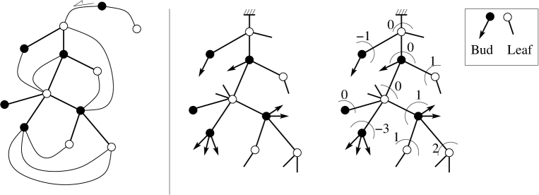
Figure 3: A bipartite map; a blossom tree rooted at a leaf, and the charge at each subtree.

Let us give a brief description of these blossom trees that are at the heart of bipartite maps. An example is provided by Figure 3. As one can expect, these trees are themselves bicolored: all the neighbours of a black vertex are white, and vice-versa. In addition to the standard vertices and edges, blossom trees carry half-edges, which are called leaves when they hang from a white vertex, and buds otherwise. Leaves are represented in our figures by short segments, while buds are represented by black outgoing arrows. The trees are rooted at a leaf or a bud, and the vertex attached to this half-edge is called the root vertex. Finally, we define the charge of a tree to be the difference between the number of leaves and the number of buds it contains; the root half-edge does not count. The charge at a vertex is the charge of the subtree rooted at this vertex. We impose the following charge conditions on the vertices of blossom trees (except at the root vertex): all white vertices have a nonnegative charge, while all black vertices have a charge at most one. The notion of charge was introduced by Bouttier et al. in [7] for the enumeration of usual planar maps, and turns out to be also useful in the bipartite case.

Given the neat recursive structure of trees, it is not difficult to write functional equations that govern a very detailed generating function for blossom trees. Let $\mbox{\boldmath$x$}=(x_{1},x_{2},\ldots)$ and $\mbox{\boldmath$y$}=(y_{1},y_{2},\ldots)$. For $i\in\mathbb{Z}$, let $W_{i}(\mbox{\boldmath$x$},\mbox{\boldmath$y$})$ be the generating function for blossom trees rooted at a leaf such that the charge at the (white) root vertex is $i$. In this series, the variable $x_{k}$ (resp. $y_{k}$) counts white (resp. black) vertices of degree $k$. Similarly, let $B_{i}(\mbox{\boldmath$x$},\mbox{\boldmath$y$})$ be the generating function for blossom trees rooted at a bud such that the charge at the (black) root vertex is $i$. Let us form the following generating functions:

$$W(\mbox{\boldmath$x$},\mbox{\boldmath$y$};z)\equiv W(z)=\sum_{i\geq 0}W_{i}(\mbox{\boldmath$x$},\mbox{\boldmath$y$})\,z^{i}\quad\hbox{ and }\quad\quad B(\mbox{\boldmath$x$},\mbox{\boldmath$y$};z)\equiv B(z)=\sum_{i\leq 1}B_{i}(\mbox{\boldmath$x$},\mbox{\boldmath$y$})\,z^{i}.$$ (1)

Then

$$W(z)=[z^{\geq 0}]\sum_{k\geq 0}x_{k+1}\Big{(}z+B(z)\Big{)}^{k},$$ (2)

and

$$B(z)=[z^{\leq 1}]\sum_{k\geq 0}y_{k+1}\left(\frac{1}{z}+W(z)\right)^{k}.$$ (3)

We have used the following notation: for any power series $S$ in $x$ and $y$ having coefficients in $\mathbb{Z}[z,1/z]$, the series $[z^{\geq 0}]S(\mbox{\boldmath$x$},\mbox{\boldmath$y$};z)$ is obtained by selecting from $S$ the terms with a nonnegative power of $z$. The notation $[z^{\leq 1}]$ naturally corresponds to the extraction of terms in which the exponent of $z$ is at most one. More generally, for any $i\in\mathbb{Z}$,

$$B_{i}(\mbox{\boldmath$x$},\mbox{\boldmath$y$})=[z^{i}]\sum_{k\geq 0}y_{k+1}\left(\frac{1}{z}+W(z)\right)^{k}.$$ (4)

Our central theorem gives an expression for the degree generating function of bipartite planar maps. This series, denoted by $B(\mbox{\boldmath$x$},\mbox{\boldmath$y$})$, enumerates maps by their number of white and black vertices having a given degree $k$ (variables $x_{k}$ and $y_{k}$). The theorem below thus solves a combinatorial problem that has an interest of its own. Moreover, we shall see that the solutions of the Ising and hard particle models on planar maps have close connections to it.

Theorem 3

The degree generating function of bipartite planar maps rooted at a black vertex of degree $2$ is related to the generating functions of blossom trees as follows:

$$M(\mbox{\boldmath$x$},\mbox{\boldmath$y$})=y_{2}((W_{0}-B_{2})^{2}+W_{1}-B_{3}-B_{2}^{2})$$

where $W_{i}\equiv W_{i}(\mbox{\boldmath$x$},\mbox{\boldmath$y$})$ and $B_{i}\equiv B_{i}(\mbox{\boldmath$x$},\mbox{\boldmath$y$})$ are defined by (1–4).

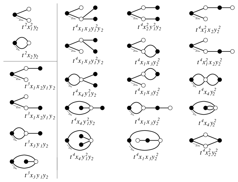
Figure 4: The bipartite maps rooted on a black vertex of degre two and having at most $4$ edges, together with their degree distribution.

Remarks
1. One can naturally write $M(\mbox{\boldmath$x$},\mbox{\boldmath$y$})=y_{2}(W_{0}^{2}+W_{1}-B_{3}-2W_{0}B_{2})$, and this expression is better suited to the applications. However, the expression of Theorem 3 will be shown to reflect more faithfully the combinatorics of maps.
2. Replacing $x_{k}$ by $t^{k}x_{k}$ gives a generating function in which edges are counted by $t$. The first few terms of $M$ then read:

$$t^{2}y_{2}(x_{1}^{2}+x_{2})+2t^{3}y_{2}y_{1}(x_{1}x_{2}+x_{3})+t^{4}y_{1}^{2}y_{2}(2x_{1}x_{3}+3x_{4}+x_{2}^{2})+t^{4}y_{2}^{2}(4x_{1}x_{3}+2x_{1}^{2}x_{2}+2x_{4}+x_{2}^{2})+O(t^{5}).$$

The corresponding bipartite maps are shown in Figure 4. Theorem 3 will be proved in Section 5.
3. Let us rephrase the above result in terms of permutations. A bipartite planar map with $n$ labelled edges can be encoded by a pair of permutations $(\sigma,\tau)$ of $\mathcal{S}_{n}$ satisfying the following conditions: the group generated by $\sigma$ and $\rho$ acts transitively on $\{1,\ldots,n\}$, and the three permutations $\sigma$, $\rho$ and $\sigma\rho$ have a total of $n+2$ cycles [11]. The enumeration of such minimal transitive factorizations is the subject of a vast litterature; see [5, 15] and references therein. For $\lambda$ and $\mu$ two partitions of $n$, let $m(\lambda,\mu)$ be the number of pairs of permutations $(\sigma,\rho)$ of respective cyclic type $\lambda$ and $\mu$, satisfying the two conditions indicated above. Theorem 3 gives an expression for the generating function $M(\mbox{\boldmath$x$},\mbox{\boldmath$y$})=\sum_{n\geq 1}\sum_{\lambda,\mu}m(\lambda,\mu)\cdot 2m_{2}\cdot\mbox{\boldmath$x$}^{\lambda}\mbox{\boldmath$y$}^{\mu}/n!$, where the inner summation is on all partitions $\lambda=1^{\ell_{1}}\ldots n^{\ell_{n}}$ and $\mu=1^{m_{1}}\ldots n^{m_{n}}$ of $n$, and the weights $\mbox{\boldmath$x$}^{\lambda}\mbox{\boldmath$y$}^{\mu}$ are defined by $\mbox{\boldmath$x$}^{\lambda}=x_{1}^{\ell_{1}}\cdots x_{n}^{\ell_{n}}$, and $\mbox{\boldmath$y$}^{\mu}=y_{1}^{m_{1}}\cdots y_{n}^{m_{n}}$.

The paper is organized as follows: in Section 3, we describe a general connection between maps and trees: one transforms a map into a tree by cutting certain of its edges into two half-edges. Conversely, merging half-edges of a tree gives a planar map. In Section 4, we show that these transformations, restricted to certain classes of maps and trees (called balanced trees) are one-to-one. Balanced trees are then enumerated in Section 5: this proves our central Theorem 3 above. Finally, Sections 6 and 7 are respectively devoted to applications of this theorem to the solution of the hard particle and Ising models.

3 Maps and trees

Take a bipartite planar map $M$ rooted at a black vertex $v$ of degree $2$. These maps are exactly those we wish to count (Theorem 3). Let us consider that each of the edges that start from $v$ is made of two half-edges. Delete $v$ and the two half-edges attached to it. Two cases occur (Figure 5):

• either we get an ordered pair of maps, each of them carrying a half-edge (or leg), on which it is rooted,

• or we get a single map with two half-edges, and root the map at the half-edge belonging to the root edge of $M$.

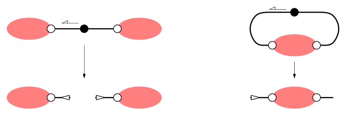
Figure 5: The deletion of a black root vertex of degree $2$.

The degree generating function of bipartite maps rooted at a black vertex of degree $2$ can thus be written as

$$M(\mbox{\boldmath$x$},\mbox{\boldmath$y$})=y_{2}(L_{1}(\mbox{\boldmath$x$},\mbox{\boldmath$y$})^{2}+L_{2}(\mbox{\boldmath$x$},\mbox{\boldmath$y$})),$$ (5)

where the series $L_{1}$ and $L_{2}$ respectively count by their degree distribution maps with one or two legs, rooted at a leg. The reason why we keep the legs is that we do not want to modify the degrees of the vertices. Compare Equation (5) to Theorem 3: the next three sections are devoted to proving that $L_{1}=W_{0}-B_{2}$ and $L_{2}=W_{1}-B_{3}-B_{2}^{2}$.

The above decomposition explains why, as in [7], we shall be interested in generalized bipartite maps, that do not only consist of the traditional edges and vertices, but also contain a number of half-edges in their infinite face (when drawn on the plane), and are rooted at one of these half-edges. Let us insist on the distinction between a half-edge, which is incident to only one vertex, and a dangling edge, which is incident to two vertices, one of which has degree one. From now on, in this section and the next two, all maps are bipartite and rooted at a half-edge. This requires, unfortunately, to introduce a bit of terminology. In passing, we shall reformulate slightly the definition of blossom trees given in Section 2.

The vertex adjacent to the root half-edge is called the root vertex of the map. Half-edges that hang from black vertices are called buds and are represented in our figures by black outgoing arrows. Half-edges that hang from white vertices are called leaves and are represented by short segments. The degree distribution of a map is the pair of partitions $(\lambda,\mu)$ such that $\lambda$ gives the degree distribution of white vertices and $\mu$ gives the degree distribution of black vertices. Half-edges are included in the degree of the vertex they are attached to. A map with $b$ buds and $\ell$ leaves obviously satisfies $b+|\lambda|=\ell+|\mu|$ where $|\lambda|$ denotes the sum of the parts of $\lambda$. The $1$-leg map of Figure 6 has degree distribution $\lambda=2^{2}345$, $\mu=24^{2}5$.

Let us now define two important subclasses of maps. A $k$-leg map is a map with exactly $k$ leaves and no bud; hence a $k$-leg map is rooted at one of its leaves. A tree is a map with only one face (and an arbitrary number of buds and leaves). The total charge of a tree is the difference between its number of leaves and its number of buds; the root half-edge is counted. The charge of a tree is the same difference, but the root half-edge is not counted. Hence the charge and total charge always differ by $\pm 1$.

Take a tree $T$ and an edge $e$ of this tree. Cut $e$ into two half-edges: this leaves two subtrees, rooted at these half-edges. The subtree that does not contain the root of $T$ is called the lower subtree of $T$ at $e$. Let $T^{\bullet}_{e}$ denote the subtree containing the black endpoint of $e$ and $T^{\circ}_{e}$ the other one. The charges $c_{\circ}$ of $T_{e}^{\circ}$ and $c_{\bullet}$ of $T_{e}^{\bullet}$ satisfy $c_{\circ}+c_{\bullet}=c$, where $c$ is the total charge of $T$. The black charge rule is satisfied at $e$ if the subtree $T_{e}^{\bullet}$ has charge at most one. The white charge rule is satisfied at $e$ if the subtree $T_{e}^{\circ}$ has a nonnegative charge.

A tree is called a blossom tree if all its lower subtrees satisfy the charge rule corresponding to their color. An example is displayed on Figure 3. The series $W_{i}$ and $B_{i}$ defined by (1–4) respectively count blossom trees of charge $i$ rooted at a leaf and a bud. The following lemma, immediate in the case $m=1$, will prove useful later on.

Lemma 4

Let $T$ be a tree of total charge one, and let $e$ be an edge of $T$. Then the black charge rule is satisfied at $e$ if and only if the white charge rule is satisfied at $e$.

If, in addition, $T$ is a blossom tree, then both charge rules are satisfied at every edge; re-rooting $T$ at another half-edge yields again a blossom tree.

3.1 Balanced trees and their closure

In this section we define the closure as a mapping $\phi$ from certain blossom trees with total charge $k\geq 1$ to $k$-leg maps. This closure is the same as in earlier texts using the idea of conjugacy classes of trees [5, 7, 20, 21, 22, 23].

Let $T$ be a tree with total charge $k\geq 1$. Its half-edges form a cyclic sequence around the tree in counterclockwise direction. Buds and leaves can be matched in this cyclic sequence as if they were respectively opening and closing brackets. More precisely, first match the pairs made of a bud and a leaf that are immediately consecutive in the cyclic sequence. Then, forget matched buds and leaves, and repeat until there is no more possible matching. In view of the number of buds and leaves in the original cyclic sequence, $k$ leaves remain unmatched. These leaves are called the single leaves of $T$.

A tree rooted at a leaf is said to be balanced if its root is single. The closure of a balanced tree $T$ is obtained as follows: match buds and leaves into pairs as previously explained and fuse each pair into an edge (in counterclockwise direction around the tree). The root remains unchanged. We thus have:

Proposition 5

Let $T$ be a balanced tree having total charge $k$ and degree distribution $(\lambda,\mu)$. Then $\phi(T)$ is a $k$-leg map with degree distribution $(\lambda,\mu)$.

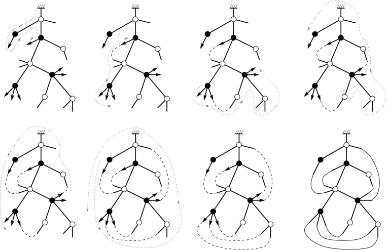
Figure 6: The closure of a balanced tree.

There is an alternative description of the closure as an iterative process, illustrated by Figure 6: start from a balanced tree $T$ and walk around the infinite face in counterclockwise order; each time a bud is immediately followed by a leaf in the cyclic sequence of half-edges, fuse them into an edge in counterclockwise direction (this creates a new finite face that encloses no unmatched half-edges); stop the course when all buds have been matched. Observe that this process may in general require to turn several times around the tree. A more efficient method is to use a stack (that is, a first-in-last-out waiting line): store buds in the stack as they are met and match leaves as they are met with the first bud available in the stack. While this is algorithmically more effective, we shall content ourselves with the previous simpler description.

3.2 The opening of a $k$-leg map

In this section we define the opening $\psi$ as a mapping from $k$-leg maps to trees with total charge $k$.

The opening of a map is the result of an iterative procedure: start from a $k$-leg map $M$ and walk around the infinite face in counterclockwise order, starting from the root; each time a non-separating edge has just been visited from its black endpoint to its white endpoint, cut this edge into two half-edges: a bud at the black endpoint and a leaf at the white endpoint; proceed until all edges are separating edges. An example is shown on Figure 7. The opening process cannot get stuck: as long as there are non-separating edges, a positive even number of them are incident to the infinite face; half of them are oriented from black to white in the counterclockwise direction. The final result is then a tree rooted at a leaf.

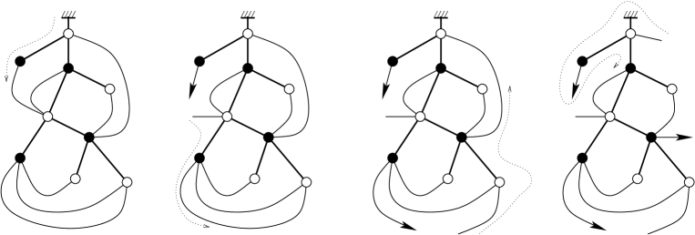
Figure 7: The first few steps of the opening of a 1-leg map. The final tree will be the one of Figure 6.

In view of the number of buds and leaves created, the image $T=\psi(M)$ of a $k$-leg map is a tree with total charge $k$. Moreover, the pairs of buds and leaves created by the opening are in correspondence in the matching procedure of the tree, so that the tree is balanced. Hence the proposition:

Proposition 6

The closure is inverse to the opening: for any $k$-leg map $M$, $\phi(\psi(M))=M$.

We shall prove below that the tree $\psi(M)$ created by the opening of a map is not only balanced, but is also a blossom tree; that is, all its lower subtrees satisfy the charge rules.

4 Bijections between maps and balanced blossom trees

4.1 The fundamental case of one-leg maps

Theorem 7

Closure and opening are inverse bijections between balanced blossom trees of total charge $1$ and $1$-leg maps. Moreover they preserve the degree distribution $(\lambda,\mu)$.

In order to prove Theorem 7, we first exhibit a bijective decomposition of $1$-leg maps into one or two smaller $1$-leg maps. Then, we present a related decomposition of balanced blossom trees of total charge $1$. We observe that the two decompositions are isomorphic, so that they induce a recursive bijection between $1$-leg maps and balanced blossom trees of total charge $1$. This bijection preserves the degree distribution. Once the existence of a bijection has thus been established, we want to identify it as the opening of maps. We observe that the opening transforms the decomposition rules of maps into the decomposition rules of trees. In view of Propositions 5 and 6, this proves that closure and opening realize this recursive bijection.

4.1.1 Decomposition of one-leg maps

We partition the set $\cal M$ of one-leg maps into four disjoint subsets and define a bijective decomposition for each of these subsets, as illustrated by Figure 9. We associate two parameters with each map $M$: its degree distribution $(\lambda,\mu)$, and the reduced degree of its infinite face, denoted by $d(M)$ (reduced means that the root leaf is not counted, so that $d(M)$ is even). These parameters will be used to check that the recursive decomposition of one-leg maps is isomorphic to that of balanced blossom trees given further.

The four subsets are defined by considering the first and second edge $e_{1}$ and $e_{2}$ that are met when walking around the infinite face in counterclockwise direction, starting from the root. We denote by $M_{0}$ the map reduced to a single vertex with one leg. We denote by ${\cal M}^{+}$ the set ${\cal M}\setminus\{M_{0}\}$.

• $M=M_{0}$. This is the base case, where the recursive decomposition stops. The infinite face of $M_{0}$ has reduced degree zero.

• $M\in\mathcal{M}_{1}$: $e_{1}$ is a dangling edge. Let $r_{1}(M)$ be the map obtained from $M$ by removing $e_{1}$ and its black endpoint.

  The mapping $r_{1}$ is a bijection from $\mathcal{M}_{1}$ to $\mathcal{M}$. Moreover $d(M)=d(r_{1}(M))+2$.

• $M\in\mathcal{M}_{2}$: $e_{1}$ is not dangling and $e_{2}$ is a separating edge. Detach $e_{2}$ from its black endpoint and turn it into a leaf $e^{\prime}_{2}$; two components remain: a one-leg map $M_{1}$ rooted at the root leaf of $M$, and a one-leg map $M_{2}$ rooted at the new leaf $e^{\prime}_{2}$. Let $r_{2}(M)=(M_{1},M_{2})$.

  The mapping $r_{2}$ is a bijection from $\mathcal{M}_{2}$ to $\mathcal{M}^{+}\times\mathcal{M}$. Moreover, $d(M)=d(M_{1})+d(M_{2})+2$.

• $M\in\mathcal{M}_{3}$: $e_{1}$ is not dangling and $e_{2}$ is not a separating edge. Let $M^{\prime}$ be obtained as follows: delete the root leaf of $M$, detach $e_{2}$ from its black endpoint, turn it into a leaf $e^{\prime}_{2}$, and re-root the map on this new leaf $e^{\prime}_{2}$. Let $r_{3}(M)=(d(M),M^{\prime})$. Observe that $d(M^{\prime})\geq d(M)$.

  The mapping $r_{3}$ is a bijection from $\mathcal{M}_{3}$ onto the set $\{(d,M^{\prime})\mid M^{\prime}\in\mathcal{M}^{+},\ d\ \hbox{even},\ 2\leq d\leq d(M^{\prime})\}$. This mapping is reversible, since the value of $d$ tells us where to create the new root.

 

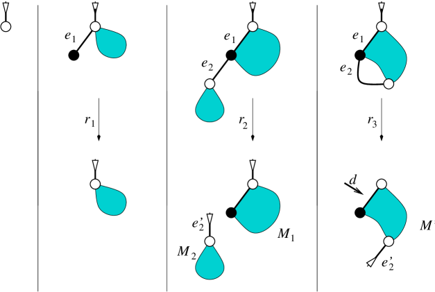
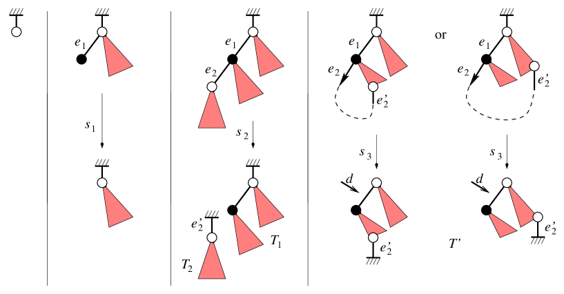
Figure 8: The decomposition of one-leg maps.

Figure 9: The decomposition of balanced blossom trees of total charge 1.

4.1.2 Decomposition of balanced blossom trees with total charge one

We partition the set $\cal T$ of balanced blossom trees of total charge one into four disjoint subsets and define a bijective decomposition for each of these subsets, as illustrated by Figure 9. The two parameters we retain for a tree $T$ are again its degree distribution $(\lambda,\mu)$, and the reduced degree of the closure of $T$, that is, $\delta(T):=d(\phi(T))$.

The four subsets of trees are defined by examining the first and second edges or half-edges $e_{1}$ and $e_{2}$ that are met when walking around the infinite face in counterclockwise direction, starting from the root. We denote by $T_{0}$ the tree reduced to a vertex with a root leaf, and by $\mathcal{T}^{+}$ the set $\mathcal{T}\setminus\{T_{0}\}$.

• $T=T_{0}$. This is the base case, where the recursive decomposition stops. The infinite face of $\phi(T)$ has reduced degree zero.

• $T\in\mathcal{T}_{1}$: $e_{1}$ is a dangling edge. Let $s_{1}(T)$ be the tree obtained from $T$ by removing $e_{1}$ and its black endpoint.

  The mapping $s_{1}$ is a bijection from $\mathcal{T}_{1}$ to $\mathcal{T}$. Moreover $\delta(T)=\delta(s_{1}(T))+2$.

• Observe that $e_{1}$ cannot be a leaf, since $T$ is balanced and has only one single leaf.

• $T\in\mathcal{T}_{2}$: $e_{1}$ is not dangling and $e_{2}$ is not a bud. Detach $e_{2}$ from its black endpoint and turn it into a leaf $e^{\prime}_{2}$; two components remain, a tree $T_{1}$ rooted at the root leaf of $T$, and a second tree $T_{2}$ rooted at the new leaf $e^{\prime}_{2}$ (with the notations used at the beginning of this section, $T_{2}=T^{\circ}_{e_{2}}$). Let $s_{2}(T)=(T_{1},T_{2})$.

  We wish to prove that $T_{1}$ and $T_{2}$ are balanced blossom trees of total charge one. Recall that $T$ is balanced, and examine the closure of $T$. Since the subtree $T_{2}$ immediately follows the root in the infinite face of $T$, no bud of $T_{1}$ can be matched to a leaf of $T_{2}$. Moreover, none of the leaves of $T_{2}$ is single in $T$ (since $T$ has a unique single leaf, which is its root). Therefore, all leaves of $T_{2}$ are matched to buds of $T_{2}$ in the closure of $T$. Since $T$ is a blossom tree, the charge of $T_{2}$ is nonnegative, so that no bud of $T_{2}$ can match a leaf of $T_{1}$. In other words, the closure takes place independently in $T_{1}$ and $T_{2}$. This proves that $T_{1}$ and $T_{2}$ are balanced, and have total charge $1$ (and hence charge $0$). In particular, the lower charge at $e_{1}$ is not modified in the transformation, and $T_{1}$ and $T_{2}$ are blossom trees.

  Hence, the mapping $s_{2}$ is a bijection from $\mathcal{T}_{2}$ to $\mathcal{T}^{+}\times\mathcal{T}$. Moreover, $\delta(T)=\delta(T_{1})+\delta(T_{2})+2$.

• $T\in\mathcal{T}_{3}$: $e_{1}$ is not dangling and $e_{2}$ is a bud. Let $e^{\prime}_{2}$ be the leaf to which $e_{2}$ is matched in the closure $\phi(T)$. Let $s_{3}(T)=(\delta(T),T^{\prime})$ where $T^{\prime}$ is obtained from $T$ by deleting the root leaf and the bud $e_{2}$, and re-rooting the tree on the leaf $e^{\prime}_{2}$.

  The tree $T^{\prime}$ is clearly balanced, and has total charge $1$. We wish to check that it satisfies the charge rules of blossom trees. According to Lemma 4, the tree obtained by re-rooting $T$ at $e^{\prime}_{2}$ satisfies both charge rules at every edge, so that it is sufficient to consider the effect of deleting the bud $e_{2}$ and the root leaf of $T$. Since these two deleted half-edges are incident to $e_{1}$, this edge is the only one where the charges are modified. Let $i\geq 0$ be the charge of $T^{\circ}_{e_{1}}$. Then $T^{\bullet}_{e_{1}}$ has charge $1-i$, and the charges of $T^{\prime\circ}_{e_{1}}$ and $T^{\prime\bullet}_{e_{1}}$ are respectively $i-1$ and $2-i$. It is thus sufficient to prove that $i\geq 1$. If $i$ was equal to $0$, a bud of $T_{1}$ would match the root leaf of $T$, which would not be balanced.

  Observe that $\delta(T^{\prime})\geq\delta(T)$. The mapping $s_{3}$ is a bijection from $\mathcal{T}_{3}$ onto the set $\{(d,T^{\prime})\mid T^{\prime}\in{\cal T}^{+},\ d\ \hbox{even},2\leq d\leq\delta(T^{\prime})\}$. The value of $d$ indicates the position of the edge $e_{1}$ in the infinite face of the closure $\phi(T^{\prime})$.

Comparing Figures 6 and 7 shows that the degree distribution $(\lambda,\mu)$ is altered in the same way by both decompositions: this proves the existence of a recursive bijection between $1$-leg maps and balanced blossom trees of total charge $1$, preserving the degree distribution. It is then an easy task to check that the opening procedure transforms the decomposition rules of maps into the decomposition rules of trees, and this completes the proof of Theorem 7.

4.2 $2$-leg maps and other extensions

Theorem 7 extends to balanced blossom trees of total charge $2$ and $2$-leg maps.

Theorem 8

There is a bijection between balanced blossom trees of total charge $2$ and $2$-leg maps. Moreover this bijection preserves the degree distribution $(\lambda,\mu)$.

Proof. Take a balanced blossom tree $T$ of total charge $2$. Observe that, apart from its root $r$, another leaf $e_{1}$ is single and ends up in the infinite face of the map $\phi(T)$ when closing the edges of $T$. Replace $r$ by an edge ending with a marked black vertex of degree $1$, and re-root the resulting tree $T^{\prime}$ at $e_{1}$. The tree $T^{\prime}$ has total charge $1$ and is still a blossom tree according to Lemma 4. Moreover the pairs of buds and leaves that are matched by closure are the same in $T^{\prime}$ as in $T$ (the closure does not depend on the root). In particular $r$ and $e_{1}$ are left untouched in the infinite face. Closure followed by re-rooting is thus a bijection between balanced blossom trees of total charge $2$, and balanced blossom trees of total charge $1$ with a marked black vertex of degree $1$ which ends up in the infinite face of $\phi(T^{\prime})$ when the edges of $T^{\prime}$ are closed. Theorem 8 is therefore a mere consequence of Theorem 7.

 

The extension to maps with more than two legs is harder but the following result will be sufficient for our purpose.

Theorem 9

Let $m\geq 3$ be an integer. Closure and opening are inverse bijections between balanced blossom trees of total charge $m$ in which the degrees of vertices are all multiples of $m$, and $m$-leg maps satisfying the same condition. Moreover the degree distribution $(\lambda,\mu)$ is preserved.

The proof of this theorem is based on a simple lemma.

Lemma 10

Let $T$ be a blossom tree in which the degrees of all vertices are multiples of $m$. Let $T^{\prime}$ be obtained from $T$ by replacing up to $m-1$ non-root leaves of $T$ by edges ending with a black vertex. Then $T^{\prime}$ is still a blossom tree.

Proof. Let $T$ be a tree in which the degrees of all vertices are multiples of $m$. Let $(\lambda,\mu)$ denote the vertex distribution of $T$, and observe that $m$ divides $|\lambda|$ and $|\mu|$. Then $m$ also divides the total charge of $T$, because the latter is the difference between the number $n_{\ell}$ of leaves and $n_{b}$ of buds, which satisfy $n_{b}+|\lambda|=n_{\ell}+|\mu|$.

Assume moreover that $T$ is a blossom tree. Then any lower subtree $T^{\circ}_{e}$ of $T$ has by definition a charge $c_{\circ}\geq 0$. According to the previous discussion the total charge $c_{\circ}+1$ of $T^{\circ}_{e}$ is divisible by $m$ so that in fact $c_{\circ}\geq m-1$. Since replacing a leaf by an edge ending with a black vertex decreases the charge by one, up to $m-1$ leaves can be replaced without any risk to violate a white charge rule.

 

Proof of Theorem 9. Let $T$ be a balanced blossom tree of total charge $m$ in which the degrees of vertices are multiples of $m$. Observe that its $m$ single leaves (among which the root) end up in the infinite face of the map $\phi(T)$ when closing the edges of $T$. Replace each of the single leaves of $T$ (except the root) by an edge ending with a black vertex of degree $1$. This gives, according to the previous lemma, a balanced blossom tree $T^{\prime}$ of total charge $1$, having $m-1$ marked black vertices of degree $1$ which end up in the infinite face of $\phi(T^{\prime})$ when we close the edges of $T^{\prime}$. This transformation is again a bijection, so that Theorem 9 now follows from Theorem 7.

 

The following interesting variation was observed, in the non-bipartite case, by P. Zinn-Justin [28] and by Bouttier et al. [7]. It describes a class of maps that are in bijection with trees not subject to any balance conditions – and hence, much easier to count.

Theorem 11

There is a one-to-one correspondence between (not necessarily balanced) blossom trees of charge $1$ rooted at a leaf and $1$-leg maps having a marked black vertex of degree $1$.

Similarly, there is a one-to-one correspondence between blossom trees of charge $1$ rooted at a bud and $1$-leg maps having a marked white vertex of degree $1$.

Proof. Consider a blossom tree of total charge $2$. Replace the root leaf by a marked black vertex of degree $1$ and re-root the resulting tree of charge one on its unique single leaf. The closure then yields bijectively a $1$-leg map with a marked black vertex of degree $1$. A similar argument proves the second statement.

 

5 Counting balanced trees

In view of Eq. (5) and Theorems 7 and 8, our objective is now to count balanced blossom trees of total charge $1$ or $2$. In this section, we establish bijections that allow us to express their generating functions in terms of the generating functions $W_{i}$ and $B_{i}$ of (not necessarily balanced) blossom trees. These bijections are adaptations to the bipartite case of the bijections presented in [7].

For $i\in\mathbb{Z}$, let $\mathcal{W}_{i}$ be the set of blossom trees of charge $i$ rooted at a leaf (so that the total charge is $i+1$). Similarly, let $\mathcal{B}_{i}$ be the set of blossom trees of charge $i$ rooted at a bud (their total charge is $i-1$). These trees are respectively counted by the series $W_{i}$ and $B_{i}$ of Eqs. (1–4). Finally, for $i\geq 1$, let $\mathcal{W}_{i}^{*}$ be the subset of $\mathcal{W}_{i}$ formed of balanced trees. We are especially interested in the enumeration of the trees of $\mathcal{W}_{0}^{*}$ and $\mathcal{W}_{1}^{*}$. The theorem below implies our Theorem 3 on the enumeration of bipartite maps.

Theorem 12

There exists a simple degree-preserving bijection between the sets $\mathcal{W}_{0}$ and $\mathcal{W}^{*}_{0}\cup\mathcal{B}_{2}.$ There also exists a degree-preserving bijection between the sets $\mathcal{W}_{1}$ and $\mathcal{W}^{*}_{1}\cup\mathcal{B}_{3}\cup(\mathcal{B}_{2})^{2}.$

Before proving this theorem, let us state a similar result which will allow us to count certain $m$-leg maps, with $m\geq 3$. It generalizes the results obtained in [5] for some bipartite maps called constellations.

Theorem 13

Let $m\geq 1$, and let $\widehat{\mathcal{W}}_{i}$, $\widehat{\mathcal{W}}^{*}_{i}$ and $\widehat{\mathcal{B}}_{i}$ be the restriction of the sets $\mathcal{W}_{i}$, $\mathcal{W}^{*}_{i}$ and $\mathcal{B}_{i}$ to trees in which the degrees of all vertices are multiples of $m$. There exists a simple degree-preserving bijection between $\widehat{\mathcal{W}}_{m-1}$ and $\widehat{\mathcal{W}}^{*}_{m-1}\cup\widehat{\mathcal{B}}_{m+1}.$

Proof of Theorems 12 and 13. The first bijection is extremely simple to describe: a tree $T$ belonging to $\mathcal{W}_{0}$ is either balanced (that is, belongs to $\mathcal{W}_{0}^{*}$) or its root leaf is matched to a bud. In this case, $T$ can be re-rooted at this bud; the resulting tree $T^{\prime}$ has still total charge $1$ and Lemma 4 proves that it is a blossom tree, hence an element of $\mathcal{B}_{2}$. Conversely, if we take a tree $T^{\prime}$ in $\mathcal{B}_{2}$ and re-root it at the leaf matched to the root bud, we obtain a tree of $\mathcal{W}_{0}$ that is not balanced.

We would like to have a similar argument for balanced blossom trees of total charge $2$, and, why not, of total charge $k$. What prevents us from doing so? Let us take a tree $T$ in $\mathcal{W}_{1}$: either it is balanced (that is, belongs to $\mathcal{W}_{1}^{*}$), or its root leaf is matched to a bud. In this case, let us re-root $T$ at this bud to obtain another tree $T^{\prime}$: then $T^{\prime}$ has still total charge $2$. Does $T^{\prime}$ satisfies the charge conditions? Well, not always… The following lemma describes in detail what might happen.

Lemma 14

Let $T$ be a blossom tree with total charge $k\geq 2$ and let $e$ be an edge of $T$. Denote by $c_{\bullet}$ the charge of $T^{\bullet}_{e}$ and by $c_{\circ}$ the charge of $T^{\circ}_{e}$, so that $c_{\bullet}+c_{\circ}=k$.

• If the root of $T$ belongs to $T^{\circ}_{e}$ then the black charge rule is satisfied at $e$ (that is, $c_{\bullet}\leq 1$) and the charge of $T^{\circ}_{e}$ is at least $k-1$: $c_{\circ}\geq k-1$. Hence the white charge rule is satisfied at $e$.

• If the root of $T$ belongs to $T^{\bullet}_{e}$ then the white charge rule is satisfied at $e$ (that is, $c_{\circ}\geq 0$) and the charge of $T^{\bullet}_{e}$ is at most $k$: $c_{\bullet}\leq k$. Hence the black charge rule might not be satisfied at $e$.

If $c_{\bullet}\geq 2$ the edge $e$ is called weak.

This lemma implies that if we re-root a blossom tree "on the wrong side" of a weak edge, the result will not be a blossom tree. In other words:

Lemma 15

Let $T$ be a blossom tree, and let $T^{\prime}$ be obtained by re-rooting $T$ at a half-edge $e$. Then $T^{\prime}$ is a blossom tree if and only if there is no weak edge on the path from the root of $T$ to $e$.

This leads to the notion of core, introduced in [7]: let $T$ be a blossom tree and let $S$ be the set of weak edges of $T$; the core of $T$ is the connected component of $T\setminus S$ containing the root. The above lemma can be reformulated by saying that re-rooting a blossom tree gives a blossom tree if and only if the new root as been chosen in the core. In this case, the core of the new tree coincides with that of the original tree. For trees of total charge $2$, the core can be defined without refering to the root: consider a tree $T$ with total charge $2$ that satisfies the white charge rule at every edge; let $S$ be the set of its weak edges (those having charge $2$ at their black endpoint); the core of $T$ is the unique component of $T\setminus S$ with total charge $2$. This description of the core will be useful in the sequel.

The above discussion shows that it is difficult to characterize the trees obtained by re-rooting an unbalanced blossom tree $T$ (of total charge $k\geq 2$) at the bud that matches its root: if $T$ has a non-trivial core, we might obtain a tree that is not a blossom tree.

As already exemplified by the proof of Lemma 10, the assumptions of Theorem 13 make it more difficult to violate the charge rule. Let us now prove that, under these assumptions, a blossom tree $T$ with total charge $m$ has an empty core, so that the argument used in the case $k=1$ applies again, and $\widehat{\mathcal{W}}_{m-1}$ is indeed in bijection with $\widehat{\mathcal{W}}^{*}_{m-1}\cup\widehat{\mathcal{B}}_{m+1}$. Assume that $T$ contains a weak edge $e$, that is to say, $T^{\circ}_{e}$ has a (nonnegative) charge $c_{\circ}=m-c_{\bullet}\leq m-2$ (see Lemma 14). Equivalently, $T^{\circ}_{e}$ is a blossom tree with total charge $c=c_{\circ}+1$ in the interval $[1,m-1]$. Let $n_{b}$ be the number of buds of $T^{\circ}_{e}$, $n_{\ell}=n_{b}+c$ its number of leaves and $(\lambda,\mu)$ its degree distribution. Then $n_{b}+|\lambda|=n_{b}+c+|\mu|$. But $c$ belongs to $[1,m-1]$, and this contradicts the assumption that $m$ divides both $|\lambda|$ and $|\mu|$. This concludes the proof of Theorem 13.

We are thus left with the tricky second statement of Theorem 12. It admits (at least) two proofs, or maybe two variants of the same proof. First, one can adapt the not-so-easy arguments of [7, Section 3.4 and Appendix B]. We choose instead to present an explicit bijection, that can be summarized as follows. Let us take a blossom tree $T$ in $\mathcal{W}_{1}$ having the misfortune of being unbalanced. We want to associate with it an element $\rho(T)$ belonging to $\mathcal{B}_{3}\cup(\mathcal{B}_{2})^{2}$. As before the tree $T$ is rooted on a leaf and we want to re-root it on a bud of the core. Problems arise when the bud matched to the root by the closure is not in the core. The idea is then to go across the subtrees that dangle from the core to look further away for our dream bud. This idea is schematized by Figure 10 which will be explained in greater detail below. Most of the time, we shall reach a bud of the core, and obtain a tree of $\mathcal{B}_{3}$. Sometimes we will fail to return to the core, and this will yield the term $(\mathcal{B}_{2})^{2}$.

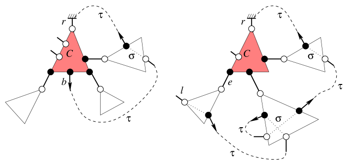
Figure 10: Chains in the graphs of $\sigma$ and $\tau$. In the first tree the root is sent to a bud of the core. In the second one the root is sent to a single leaf which is not in the core.

In order to make the construction more precise, some notations are useful. They are illustrated by Figure 10. For every tree $T_{0}$ with charge zero, let us choose a bijection $\sigma_{T_{0}}$ from its buds to its leaves, ignoring the root half-edge. This bijection may be chosen arbitrarily. Now take a tree $T$ with total charge $2$, and assume it satisfies the white charge rule at every edge (this is the case for instance if $T$ is a blossom tree). Let $C$ be the core of $T$ (defined, as above, without any reference to the root), and let $E$ be the set of weak edges incident to $C$. Each edge $e$ of $E$ defines a subtree $T_{e}^{\circ}$ of charge zero. Any vertex of $T$ is either in the core or in one of the trees $T_{e}^{\circ}$, for $e\in E$. The bijections $\sigma_{T_{e}^{\circ}}$, for $e\in E$, induce a bijection $\sigma$ between the buds and leaves that are not in the core. The closure of $T$ induces another bijection $\tau$ from its non-single leaves to its buds. Observe that $\sigma$ and $\tau$ do not depend on which half-edge is the root of $T$. The graph of the bijection $\sigma$ (resp. $\tau$) is made of oriented edges going from buds to leaves (resp. from leaves to buds). Hence the union of these two graphs is made of oriented cycles and chains on buds and leaves of $T$.

Assume now that $T$ is a blossom tree from $\mathcal{W}_{1}\setminus\mathcal{W}_{1}^{*}$. The root of $T$ is a leaf $r$ which is not in the image of $\sigma$ (it is in the core) but is in the domain of $\tau$. It is thus the origin of a chain. What is the endpoint of this chain ? There are two cases. Either the endpoint is in the image of $\tau$ but not in the domain of $\sigma$; that is, it is a bud $b$ of the core (Figure 10, left). Or the endpoint is in the image of $\sigma$ but not in the domain of $\tau$; that is, it is a single leaf $\ell$ of $T$ which is not in the core (Figure 10, right). We shall define $\rho(T)$ separately in these two cases. Let $\mathcal{W}_{b}$ be the subset of $\mathcal{W}_{1}\setminus\mathcal{W}^{*}_{1}$ of trees such that the chain starting at the root ends at a bud, and let $\mathcal{W}_{\ell}$ be the complementary subset.

First case: assume that $T$ belongs to $\mathcal{W}_{b}$. Re-rooting the tree $T$ on the endpoint $b$ yields a tree $T^{\prime}$. Since $b$ is a bud of the core, $T^{\prime}$ belongs to $\mathcal{B}_{3}$. Set $\rho(T)=T^{\prime}$. Conversely, take a tree $T^{\prime}$ of $\mathcal{B}_{3}$. Define the bijections $\sigma$ and $\tau$ as above. The union of their graphs defines cycles and chains. The root of $T^{\prime}$ is a bud of the core, hence the endpoint of a chain. The origin of this chain is a leaf $r$ of the core: indeed, these leaves are the only half-edges to be in the domain of one bijection and not in the image of the other. Re-rooting the tree $T^{\prime}$ on $r$ yields a tree $T$ of $\mathcal{W}_{b}$. Since the definitions of $\sigma$ and $\tau$ do not depend on the root, $T$ is the only tree such that $\rho(T)=T^{\prime}$. Hence $\rho$ is one-to-one between $\mathcal{W}_{b}$ and $\mathcal{B}_{3}$.

Second case: assume that $T$ belongs to $\mathcal{W}_{\ell}$, and let $\ell$ be the single leaf ending the chain that starts at the root of $T$. An example is given in Figure 11. The endpoint $\ell$ is not in the core. Therefore there is a (unique) edge $e$ of $E$ such that $\ell$ belongs to $T_{e}^{\circ}$. Let $T_{1}:=T_{e}^{\bullet}$. Then $T_{1}$ belongs to $\mathcal{B}_{2}$, by definition of $E$ and Lemma 15. Consider now $T_{e}^{\circ}$. It has charge $0$; let us prove that is it not balanced. The chain that starts from the root of $T$ and ends at the leaf $\ell$ enters $T_{e}^{\circ}$ for the first time at a bud. This bud is matched in $T$ to a leaf of $T_{e}^{\bullet}$, and this prevents $T_{e}^{\circ}$ from being balanced. Hence, re-rooting $T_{e}^{\circ}$ on the bud matched to its root yields a tree of $\mathcal{B}_{2}$, which we denote by $T_{2}$.

Let us consider the closure of $T$ (Figure 11). Let us denote by $j_{1}-1$ the number of buds of $T_{e}^{\bullet}$ that are matched to a leaf of $T_{e}^{\circ}$. Observe that, in the closure of $T_{e}^{\bullet}$, the root vertex of $T_{e}^{\bullet}$ lies at depth $j_{1}$. Let $j_{1,2}$ be the number of buds of $T_{e}^{\circ}$ that are matched to a leaf of $T_{e}^{\bullet}$. Let $j_{2,2}$ be the number of buds of $T_{e}^{\circ}$ that are matched to a leaf of $T_{e}^{\circ}$, in such a way the matching edge goes around the root of $T$ before ending at a leaf of $T_{e}^{\circ}$. Finally, let $j_{2}=j_{1,2}+j_{2,2}$. In the closure of $T_{e}^{\circ}$, the root vertex of $T_{e}^{\circ}$ lies at depth $j_{2}$. Observe that, if the second single leaf of $T$ is in $T_{e}^{\bullet}$, then $j_{2,2}=0.$ Since $T_{e}^{\circ}$ has charge $0$, counting leaves and buds gives $j_{2}=j_{1}-1+j_{2,2}+s$, where $s\in\{1,2\}$ is the number of single leaves of $T$ that lie in $T_{e}^{\circ}$. Consequently, $j_{1}\leq j_{2}$, and the equality holds if and only if the second single leaf of $T$ is in $T_{e}^{\bullet}$.

If $\ell^{\prime},\ell$ and $e$ appear in this order in counterclockwise direction around $T_{e}^{\circ}$, set $\rho(T)=(T_{2},T_{1})$. In all other cases (and in particular if $\ell^{\prime}$ is in $T_{e}^{\bullet}$), set $\rho(T)=(T_{1},T_{2})$. Either ways, $\rho(T)$ belongs to $(\mathcal{B}_{2})^{2}$.

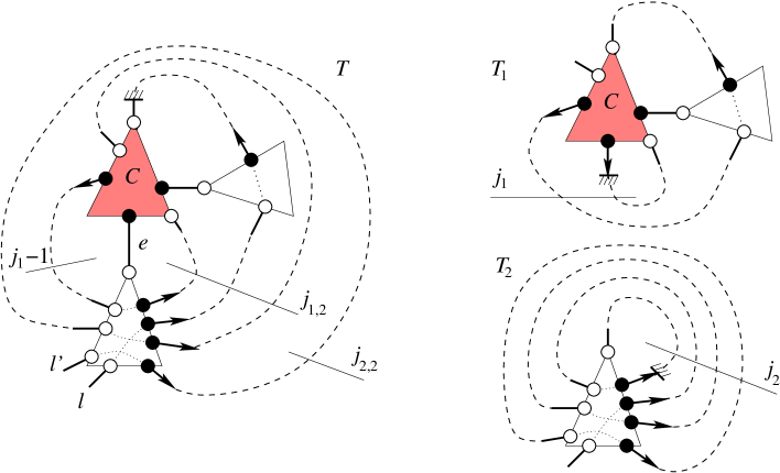
Figure 11: The decomposition of a tree $T$ of $\mathcal{W}_{\ell}$. The triple $(\ell^{\prime},\ell,e)$ appears in counterclockwise order around $T_{e}^{\circ}$, so that $\rho(T)=(T_{2},T_{1})$.

Conversely, take a pair $(T_{a},T_{b})$ of $(\mathcal{B}_{2})^{2}$. Let $j_{a}$ and $j_{b}$ be the depths of the roots of $T_{a}$ and $T_{b}$ respectively. Rename the pair $(T_{1},T_{2})$ if $j_{a}\leq j_{b}$; $(T_{2},T_{1})$ otherwise. The respective depths of the roots of $T_{1}$ and $T_{2}$ then satisfy $j_{1}\leq j_{2}$. Merge the root of $T_{1}$ with the leaf matched to the root of $T_{2}$. This creates an edge $e$ and an unrooted tree $T^{\prime}$. By construction, the tree $T^{\prime}$ satisfies the white charge rule at every edge and has total charge $2$. Let $C$ be its core and define $\sigma$ and $\tau$ as above. Consider the single leaves of $T^{\prime}$. If $j_{1}=j_{2}$ then $T_{2}$ contains exactly one of them, which we call $\ell$. Otherwise, the relation $j_{1}<j_{2}$ implies that $T_{2}$ contains both single leaves of $T$. Name them $\ell$ and $\ell^{\prime}$ so that the triple $(\ell,\ell^{\prime},e)$ appears in counterclowise direction around $T_{2}$ if the original pair $(T_{a},T_{b})$ was $(T_{1},T_{2})$; in clockwise direction otherwise. The leaf $\ell$ belongs to a chain of the union of the graphs of $\sigma$ and $\tau$, and the origin of this chain is a leaf of the core. Re-rooting on this leaf yields a tree $T$ of $\mathcal{W}_{\ell}$. Since $\sigma$ and $\tau$ are defined independently of the root, $T$ is the unique tree such that $\rho(T)=(T_{a},T_{b})$. Finally this proves that $\rho$ is one-to-one between $\mathcal{W}_{\ell}$ and $(\mathcal{B}_{2})^{2}$, and concludes the proof of Theorem 12.

 

6 Hard particle models on planar maps

In this section, we consider rooted planar maps in which some vertices are occupied by a particle, in such a way two adjacent vertices are not both occupied. The vacant (resp. occupied) vertices are represented by white (resp. black) cells. Moreover, we require the two ends of the root edge to be vacant. We shall say, for short, that the map is rooted at a vacant edge. Let $H(\mbox{\boldmath$X$},\mbox{\boldmath$Y$})$ denote the generating function for these maps, in which $X_{k}$ (resp. $Y_{k}$) counts white (resp. black) vertices of degree $k$. As above, $X$ stands for $(X_{1},X_{2},\ldots)$ and $Y$ for $(Y_{1},Y_{2},\ldots)$.

Theorem 16

The hard particle generating function for planar maps rooted at a vacant edge can be expressed in terms of the generating function for blossom trees as follows:

$$H(\mbox{\boldmath$X$},\mbox{\boldmath$Y$})=(W_{0}-B_{2})^{2}+W_{1}-B_{3}-B_{2}^{2},$$

where the series $W_{i}\equiv W_{i}(\mbox{\boldmath$x$},\mbox{\boldmath$y$})$ and $B_{i}\equiv B_{i}(\mbox{\boldmath$x$},\mbox{\boldmath$y$})$ are evaluated at $x_{k}=X_{k}$ for $k\geq 1$, $y_{2}=1+Y_{2}$ and $y_{k}=Y_{k}$ for $k\not=2$.

Proof. Take a map with hard particles. On every edge having both ends vacant, add a black vertex of degree 2, of a special shape: say, a square black vertex (Figure 12). One thus obtains a bipartite map satisfying the following conditions:

– the black vertices of degree 2 can be discs or squares,

– all other vertices are discs,

– the root vertex is a black square of degree 2.

We conclude using Theorem 3.

 

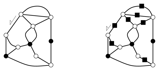
Figure 12: From a hard particle configuration to a bipartite map.

6.1 Hard particles on tetravalent maps

We apply here Theorem 16 to tetravalent maps. That is, all the variables $X_{k}$ and $Y_{k}$ are zero, except for $k=4$.

As a preliminary result, we need to enumerate blossom trees having white vertices of degree 4 and black vertices of degree 2 and 4. We are actually going to solve a slightly more general enumeration problem, by counting blossom trees having black and white vertices of degree $2$ and $4$: first because this problem is nicely symmetric, then (and most importantly) because we shall need this result to solve the Ising model on tetravalent maps.

The corresponding series $W_{i}$ and $B_{i}$ depend on the four variables $x_{2}$, $y_{2}$, $x_{4}$ and $y_{4}$, which we denote below by $v$, $w$, $x$ and $y$ for the sake of simplicity. Observe that the charge at the root of such blossom trees is always odd: hence the series $W_{2i}$ and $B_{2i}$ are all zero. Equations (2) and (3) specialize to

$$\left\{\begin{array}[]{lll}W_{1}&=&v(1+B_{1})+3xB_{-1}(1+B_{1})^{2},\\ W_{3}&=&x(1+B_{1})^{3},\end{array}\right.\hskip 28.45274pt\left\{\begin{array}[]{lll}B_{-1}&=&w+3yW_{1},\\ B_{1}&=&wW_{1}+3y(W_{3}+W_{1}^{2}),\end{array}\right.$$

and $W_{5}=0$, while Equation (4) gives:

$$B_{3}=wW_{3}+yW_{1}(6W_{3}+W_{1}^{2}).$$ (6)

After a few reductions, we express all the series $W_{i}$ and $B_{i}$ in terms of the series $P=1+B_{1}$, which satisfies:

$$P=1+3xyP^{3}+\frac{P(v+3xwP)(w+3yvP)}{(1-9xyP^{2})^{2}}.$$ (7)

In particular,

$$W_{1}=\frac{P(v+3xwP)}{1-9xyP^{2}}\quad\hbox{and}\quad W_{3}=xP^{3}.$$ (8)

By Theorem 16, the hard particle generating function on tetravalent maps can be expressed in terms of the above series $W_{1}$ and $B_{3}$ with $v=0$ and $w=1$. We thus obtain the following result.

Proposition 17 (Hard particles on tetravalent maps)

The hard particle generating function for tetravalent maps rooted at a vacant edge is algebraic of degree $7$ and can be expressed as:

$$H(x,y)=xP^{3}+\frac{xP^{2}(3-2P)}{1-9xyP^{2}}-\frac{27x^{3}yP^{6}}{(1-9xyP^{2})^{3}}$$

where $P\equiv P(x,y)$ is the power series defined by

$$P=1+3xyP^{3}+\frac{3xP^{2}}{(1-9xyP^{2})^{2}}.$$

Remarks
1. This proposition is exactly Corollary 2; we have proved it without refereeing to the (more general) Ising model.
2. The parametrization by $P$ is equivalent the one given in [6] for the free energy of this hard particle model: more precisely, upon setting $x=g,y=zg$ and $P=V/g$, the equation defining the parameter $P$ becomes Eq. (2.14) of the above reference.

6.2 Hard particles on trivalent maps

We apply here Theorem 16 to trivalent (or cubic) maps. That is, all the variables $X_{k}$ and $Y_{k}$ are zero, except for $k=3$.

We first need to enumerate blossom trees having white vertices of degree 3 and black vertices of degree 2 and 3. Again, we shall solve a more symmetric problem by counting blossom trees having black and white vertices of degree $2$ and $3$. The corresponding series $W_{i}$ and $B_{i}$ depend on $x_{2}$, $y_{2}$, $x_{3}$ and $y_{3}$, which are denoted below by $v,w,x$ and $y$. This model is a bit more complex than the previous one, since now a blossom tree may have an even charge. However, Equations (2) and (3) specialize to

$$\left\{\begin{array}[]{lll}W_{0}&=&vB_{0}+x(2B_{-1}+2B_{-1}B_{1}+B_{0}^{2}),\\ W_{1}&=&v(1+B_{1})+2xB_{0}(1+B_{1}),\\ W_{2}&=&x(1+B_{1})^{2},\end{array}\right.\hskip 14.22636pt\left\{\begin{array}[]{lll}B_{-1}&=&w+2yW_{0},\\ B_{0}&=&wW_{0}+y(2W_{1}+W_{0}^{2}),\\ B_{1}&=&wW_{1}+2y(W_{2}+W_{0}W_{1}).\end{array}\right.$$

Equation (4) then gives

$$B_{2}=wW_{2}+y(2W_{0}W_{2}+W_{1}^{2})\quad\hbox{and}\quad B_{3}=2yW_{1}W_{2}.$$ (9)

Let $P=1+B_{1},Q=W_{0}$ and $R=B_{0}$. Then

$$\left\{\begin{array}[]{l}\displaystyle P=1+2xyP^{2}+P(w+2yQ)(v+2xR),\\ \\ \displaystyle(1-4xyP)Q=2xwP+R(v+xR),\\ \\ \displaystyle(1-4xyP)R=2yvP+Q(w+yQ),\end{array}\right.$$ (10)

and all the series $W_{i}$ and $B_{i}$ have simple rational expressions in terms of $P,Q,R$. In particular,

$$W_{0}=Q,\quad B_{-1}=w+2yQ,\quad W_{1}=P(v+2xR)\quad\hbox{and}\quad W_{2}=xP^{2}.$$ (11)

By Theorem 16, the hard particle generating function on trivalent maps can be expressed in terms of the above series $W_{i}$ and $B_{i}$ evaluated at $v=0$ and $w=1$. We thus obtain the following result:

Proposition 18 (Hard particles on trivalent maps)

The hard particle generating function for trivalent maps rooted at a vacant edge is algebraic of degree $11$ and can be expressed as follows:

$$H(x,y)=Q^{2}+2xPR-4x^{2}yP^{3}R-2xP^{2}Q-4xyP^{2}Q^{2}-8x^{2}yP^{2}QR^{2},$$

where $P,Q$ and $R$ are the power series defined by Eqs. (10) above, with $v=0$ and $w=1$.

Remark. Set $v=0$ and $w=1$ in (10), and eliminate $R$. This gives

$$\left\{\begin{array}[]{lll}P&=&\displaystyle 1+2xyP^{2}+\frac{2xPQ(1+yQ)(1+2yQ)}{1-4xyP},\\ \\ Q&=&\displaystyle\frac{2xP}{1-4xyP}+\frac{xQ^{2}(1+yQ)^{2}}{(1-4xyP)^{3}}.\end{array}\right.$$

This algebraic parametrization is easily ckecked to be the same as the one given in [6] for the free energy of the hard particle model on trivalent maps: more precisely, upon setting $x=g,y=gz,P=V/(zg^{2})$ and $Q=R/(zg)$, one recovers Eqs. (C.7) and (C.8) of the above reference.

7 The Ising model on planar maps

In this section, we consider maps with white and black vertices, and enumerate them according to their degree distribution (variables $X_{k}$ and $Y_{k}$) and according to the number of frustrated edges (variable $u$). Let us recall that an edge is frustrated if it has a black end and a white one.

7.1 General result

Theorem 19

The Ising generating function $I(\mbox{\boldmath$X$},\mbox{\boldmath$Y$},u)$ for planar maps whose root vertex is black and has degree $2$ can be expressed in terms of the generating functions for blossom trees:

$$I(\mbox{\boldmath$X$},\mbox{\boldmath$Y$},u)=Y_{2}(u-\bar{u})\left((W_{0}-B_{2})^{2}+W_{1}-B_{3}-B_{2}^{2}\right),$$

where the series $W_{i}\equiv W_{i}(\mbox{\boldmath$x$},\mbox{\boldmath$y$})$ and $B_{i}\equiv B_{i}(\mbox{\boldmath$x$},\mbox{\boldmath$y$})$ are evaluated at

$$\left\{\begin{array}[]{lllllll}x_{2}&=&\bar{u}+X_{2}(u-\bar{u}),\\ x_{k}&=&X_{k}(u-\bar{u})^{k/2},&\end{array}\right.\left\{\begin{array}[]{lllllll}y_{2}&=&\bar{u}+Y_{2}(u-\bar{u}),\\ y_{k}&=&Y_{k}(u-\bar{u})^{k/2},&\hbox{for }k\not=2\end{array}\right.$$

with $\bar{u}=1/u$.

Proof. Take a bicolored map rooted at a black vertex of degree 2. On each edge, add a (possibly empty) sequence of square vertices of degree 2, in such a way the resulting map is bipartite. An example is shown on Figure 13. Note that every frustrated edge receives an even number of square vertices, while every uniform edge receives an odd number of these squares. The resulting map remains rooted at its black vertex of degree 2, which is not a square.

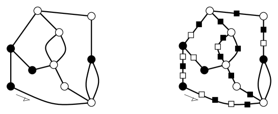
Figure 13: An Ising configuration with a black root of degree two and one of the associated bipartite maps.

Let $\tilde{M}(\mbox{\boldmath$x$},\mbox{\boldmath$y$},v)$ denote the degree generating function for the maps one obtains in that way: in this series, the square vertices are counted by $v$, while the other vertices are, as usually, counted by the variables $x_{k}$ and $y_{k}$. The above construction gives

$$\tilde{M}(\mbox{\boldmath$x$},\mbox{\boldmath$y$},v)=I(\mbox{\boldmath$X$},\mbox{\boldmath$Y$},u)$$ (12)

where

$$X_{k}=\frac{x_{k}}{(\bar{v}-v)^{k/2}},\quad Y_{k}=\frac{y_{k}}{(\bar{v}-v)^{k/2}}\quad\hbox{and}\quad u=1/v=\bar{v}.$$

By Theorem 3, we also have

$$\tilde{M}(\mbox{\boldmath$x$},\mbox{\boldmath$y$},v)=y_{2}((W_{0}-B_{2})^{2}+W_{1}-B_{3}-B_{2}^{2})$$ (13)

where the series $W_{i}$ and $B_{i}$ are evaluated at $x_{1},x_{2}+v,x_{3},\ldots,y_{1},y_{2}+v,y_{3},\ldots$ The result follows by comparison of (12) and (13).

 

7.2 The Ising model on quasi-regular maps

The general result above applies in particular to quasi-regular maps, that is, maps in which all vertices have degree $m\geq 3$, except for the root which has degree $2$. Let us make Theorem 19 explicit for the case $m=4$ (this is Proposition 1) and $m=3$ (Proposition 20 below).

For quasi-tetravalent maps, we first form the Ising generating function for planar maps, rooted at a black vertex of degree $2$, having only vertices of degree $2$ and $4$. This series is given by Theorem 19, with $X_{k}=Y_{k}=0$ for $k\not=2,4$. The blossom trees occurring in this theorem are the ones that have been counted in Section 6.1. Their enumeration has resulted in Eqs. (6–8). Theorem 19 yields:

$$I(\mbox{\boldmath$X$},\mbox{\boldmath$Y$},u)=Y_{2}(u-\bar{u})(W_{1}-B_{3}),$$

where $W_{1}$ and $W_{3}$ are evaluated at $v=\bar{u}+X_{2}(u-\bar{u})$, $w=\bar{u}+Y_{2}(u-\bar{u})$, $x=X_{4}(u-\bar{u})^{2}$, $y=Y_{4}(u-\bar{u})^{2}$. The Ising generating function for quasi-tetravalent maps is obtained by setting $X_{2}=0$ in the series $I(\mbox{\boldmath$X$},\mbox{\boldmath$Y$},u)$, and then by extracting the coefficient of $Y_{2}$: in other words, by setting $v=w=\bar{u}$ in the series $W_{1}$ and $W_{3}$. Proposition 1 follows.

The same argument gives the Ising generating function of quasi-cubic maps as

$$I(X,Y,u)=(u-\bar{u})((W_{0}-B_{2})^{2}+W_{1}-B_{3}-B_{2}^{2}),$$

where the series $W_{i}$ and $B_{i}$ are given by Eqs. (9–11) and are evaluated at $v=w=\bar{u}$, $x=X(u-\bar{u})^{3/2}$, $y=Y(u-\bar{u})^{3/2}$. We thus obtain:

Proposition 20 (Ising on quasi-cubic maps)

Let $I(X,Y,u)$ be the Ising generating function of quasi-cubic maps rooted at a black vertex. The variables $X$ and $Y$ account for the number of (cubic) white and black vertices, while $u$ counts the frustrated edges. Then

$$\frac{I(X,Y,u)}{u-\bar{u}}=Q^{2}+P(v+2xR)-2xyP^{3}(v+2xR)-2xvP^{2}Q-4xyP^{2}Q^{2}-2yP^{2}Q(v+2xR)^{2},$$

where $P,Q,R$ are the series defined by (10), evaluated at $x=X(u-\bar{u})^{3/2}$, $y=Y(u-\bar{u})^{3/2}$ and $v=w=1/u=\bar{u}$. All these series are algebraic of degree $11$.

Remarks
1. Set $w=v$ in (10), and denote $\bar{Q}=v+2yQ$, $\bar{R}=v+2xR$. Then

$$\left\{\begin{array}[]{l}\displaystyle P=1+2xyP^{2}+P\bar{Q}\bar{R},\\ \\ \displaystyle(1-4xyP)\bar{Q}=v+\frac{y}{2x}\left(\bar{R}^{2}-v^{2}\right),\\ \\ \displaystyle(1-4xyP)\bar{R}=v+\frac{x}{2y}\left(\bar{Q}^{2}-v^{2}\right).\end{array}\right.$$

The above system of equations is equivalent to the parametrization given in [4] for the free energy of the Ising model on trivalent maps. More precisely, upon setting

$$x=\frac{ge^{H}}{c^{3/2}},\quad y=\frac{ge^{-H}}{c^{3/2}},\quad v=1/c,\quad P=\frac{c^{2}z}{g^{2}},\quad\bar{Q}=-\frac{\kappa}{c},\quad\bar{R}=-\frac{\rho}{c},$$

the parametrization in $P,\bar{Q},\bar{R}$ becomes Eqs. (40–41) of Ref. [4], with $g^{2}$ replaced by $-g^{2}$.
2. Erasing the root vertex of a quasi-regular map gives an authentic regular map. Thanks to this remark, the above generating functions can also be written as

$$I(X,Y,u)=u^{2}I_{0,0}(X,Y,u)+I_{0,1}(X,Y,u)+I_{1,0}(X,Y,u)+I_{1,1}(X,Y,u),$$

where $I_{0,0}$ is the Ising generating function for $m$-regular maps rooted at a uniformly white edge, $I_{0,1}$ is the Ising generating function for $m$-regular maps rooted at a frustrated edge (oriented from its white endpoint to its black one) and so on.

7.3 The Ising model on regular maps

The general result of Theorem 19 is obviously not very convenient for solving the Ising model on truly regular $m$-valent maps, for $m\geq 3$. A re-rooting procedure circumvents this difficulty, to the cost of an expression of the Ising generating function in terms of an integral. In the tetravalent case at least, this integral can be evaluated as an algebraic function.

Suppose we are interested in the Ising enumeration of $m$-valent maps, rooted at a white vertex. We still denote by $I(X,Y,u)$ the associated generating function, where $X$ (resp. $Y$) counts white (resp. black) vertices, and $u$ counts the frustrated edges. As in Section 7.1, let us add a sequence of vertices of degree $2$ on every edge, in such a way the resulting map is bipartite, and still rooted at a white vertex of degree $m$ (Figure 14). Let $\tilde{M}(x,y,v)$ be the generating function for the maps thus obtained, where the vertices of degree 2 are counted by $v$, and the other ones by $x$ and $y$. Then

$$\tilde{M}(x,y,v)=I\left(\frac{x}{(\bar{v}-v)^{m/2}},\frac{y}{(\bar{v}-v)^{m/2}},\bar{v}\right).$$ (14)

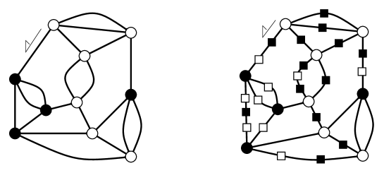
Figure 14: An Ising configuration on a tetravalent map and one of the associated bipartite maps.

Now, let $\bar{M}(x,y,v)$ be the generating function $M(\mbox{\boldmath$x$},\mbox{\boldmath$y$})$ of bipartite maps rooted at a black vertex of degree 2 (given by Theorem 3), evaluated at $x_{2}=y_{2}=v,x_{m}=x,y_{m}=y$, all the other variables $x_{k}$ and $y_{k}$ being zero. Then $\bar{M}(x,y,v)+\bar{M}(y,x,v)$ counts maps rooted at a vertex of degree 2, either black or white. In these maps, let us orient another edge, starting now from a white vertex of degree $m$: we get a doubly rooted map, which can be obtained in an alternative may, namely by orienting an edge that starts from a vertex of degree 2 in a map counted by $\tilde{M}(x,y,v)$. In algebraic terms,

$$mx\frac{\partial}{\partial x}\left(\bar{M}(x,y,v)+\bar{M}(y,x,v)\right)=2v\frac{\partial\tilde{M}}{\partial v}(x,y,v).$$

Integrating this equation provides the generating function of bipartite maps rooted at a white vertex of degree $m$ that contain at least one vertex of degree $2$:

$$\tilde{M}(x,y,v)-\tilde{M}(x,y,0)=\frac{mx}{2}\int_{0}^{v}\frac{\partial}{\partial x}\left(\bar{M}(x,y,z)+\bar{M}(y,x,z)\right)\frac{dz}{z}.$$ (15)

There remains to evaluate the generating function $\tilde{M}(x,y,0)$ for $m$-valent bipartite maps rooted at a white vertex. By deleting the black end of the root edge, together with the $m$ half-edges that are attached to it, we obtain an $m$-leg map. By Theorem 9, these maps are in bijection with $m$-regular balanced blossom trees of total charge $m$. For $m$-regular blossom trees, Eqs. (2) and (3) simply give:

$$W_{m-1}=x(1+B_{1})^{m-1}\quad\hbox{and}\quad B_{1}=(m-1)yW_{m-1},$$ (16)

while Eq. (4) gives

$$B_{m+1}=y{{m-1}\choose 2}W_{m-1}^{2}.$$

Hence Theorem 13 gives the generating function for $m$-valent bipartite maps rooted at a white vertex in the form

$$\tilde{M}(x,y,0)=yW_{m-1}^{*}=A-{{m-1}\choose 2}A^{2},$$ (17)

where $A=yW_{m-1}$ satisfies

$$A=xy(1+(m-1)A)^{m-1}.$$ (18)

By combining (14), (15) and (17), we obtain an integral expression of the Ising generating function of $m$-valent maps.

Theorem 21

The Ising generating function $I(X,Y,u)$ of $m$-valent maps rooted at a white vertex can be expressed as follows:

$$I(X,Y,u)=A-{{m-1}\choose 2}A^{2}+\frac{mx}{2}\int_{0}^{v}\frac{\partial}{\partial x}\left(\bar{M}(x,y,z)+\bar{M}(y,x,z)\right)\frac{dz}{z},$$

where the series $A\equiv A(x,y)$ is given by (18) and $\bar{M}(x,y,z)$ counts bipartite maps having only vertices of degree $2$ and $m$, rooted at a black vertex of degree $2$. Both series are evaluated at $x=X(u-\bar{u})^{m/2}$, $y=Y(u-\bar{u})^{m/2}$ and $v=1/u=\bar{u}$.

As an application of this general result, we shall now solve the Ising model on truly tetravalent maps. We shall see that, in this case, the series $I(X,Y,u)$ is itself algebraic, and belongs to the same extension of $\mathbb{Q}[X,Y,u]$ as $\bar{M}(x,y,v)$. We expect this to be always true: the nature of a map generating function should not depend on details of the choice of the root.

Proposition 22 (Ising on tetravalent maps)

Let $I(X,Y,u)$ be the Ising generating function for bicolored tetravalent maps rooted at a white vertex. Let $P(x,y,v)$ be the power series defined by the following algebraic equation:

$$P=1+3xyP^{3}+v^{2}\frac{P(1+3xP)(1+3yP)}{(1-9xyP^{2})^{2}}.$$

Then $I(X,Y,u)$ can be expressed in terms of $P(x,y,v)$, with $x=X(u-\bar{u})^{2},y=Y(u-\bar{u})^{2}$ and $v=\bar{u}=1/u$. One possible expression is:

$$I(X,Y,u)=\frac{1}{9}\Big{(}135x^{2}y^{2}P^{6}+72xy^{2}P^{5}-3y(15x+8y-3v^{2}y+36xy)P^{4}\hskip 142.26378pt$$

$$\hskip 85.35826pt-y(32+3v^{2}-36x-36y)P^{3}-(3+2v^{2}-72y)P^{2}+12(1-3y)P-9\Big{)}$$

$$\hskip 227.62204pt+\frac{(1-P-yP^{2})(1+3yP)(12-8P+3v^{2}P)}{9(1+3xP)}.$$

As $P$ itself, the series $I(X,Y,u)$ is algebraic of degree $7$.

Proof. To begin with, we have to count blossom trees having only vertices of degree $2$ and $4$. This has been done in Section 6.1, and has resulted in Eqs. (6–8). We only need the case $w=v$, which gives the above parametrization for $P$.

We shall now merely sketch the rest of the computation, for which it is useful to use a computer algebra software, like Maple. From Theorem 3, we obtain an expression of the generating function $\bar{M}(x,y,v)$ that counts bipartite maps rooted at a black vertex of degree $2$ in terms of the above parameter $P$. We then compute the derivatives of $P$ with respect to $x$ and $v$. Both derivatives are rational functions of $x,y,v$ and $P$. Observe that, from the equation defining $P$, we can express any even function of $v$ in terms of $x,y$ and $P$.

However, the integrand occurring in Theorem 21 is an odd function of $v$ (or $z$…). But so is the derivative of $P$ with respect to $v$. The combination of these two remarks allow us to write the integrand in the form

$$\frac{N(x,y,P)}{D(x,y,P)}\ \frac{\partial P}{\partial z}(x,y,z),$$

where $N$ and $D$ are polynomials in $x,y$ and $P$, not involving $z$. Hence the integral becomes

$$\int_{P(x,y,0)}^{P(x,y,v)}\frac{N(x,y,p)}{D(x,y,p)}dp.$$

The integrand is now an explicit rational function, and its primitive turns out to be rational too. Hence the integral of Theorem 21 is a rational function of $x,y,P(x,y,v)$ and $P(x,y,0)$. But the series $P(x,y,0)$ is closely related to the series $A$: indeed, $P(x,y,0)-1\equiv B_{1}(x,y,0)$ counts blossom trees with regular $4$-valent vertices, so that $P(x,y,0)=1+3A$ (see (16)). The terms involving $A$ miraculously vanish in the expression of $I(X,Y,u)$, and we end up with the not-so-simple, but algebraic, formula of Proposition 22.

 

Remarks
1. The above equation defining $P(x,y,v)$ is equivalent to the parametrization given in [4] for the free energy of the Ising model on tetravalent maps. More precisely, upon setting

$$x=\frac{-ge^{H}}{c^{2}},\quad y=\frac{-ge^{-H}}{c^{2}},\quad v=1/c\quad\hbox{and}\quad P=-{c^{2}z}/(3g),$$

the above parametrization in $P$ becomes Eq. (17) of Ref. [4].

2. Set $X=tX$ and $Y=tY$, so that $t$ counts the number of vertices. Then

$$I(tX,tY,u)=t(2X)+t^{2}(9X^{2}+XY(8u^{2}+u^{4}))+O(t^{3}).$$

The corresponding Ising configurations are shown on Figure 15.

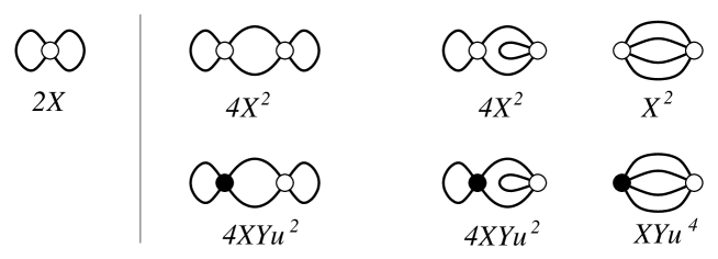
Figure 15: The (unrooted) tetravalent maps at least one white vertex (and a most two vertices). The multiplicities give the number of ways to root at a white vertex, and each rooted map is then weighted as in $I(X,Y,u)$.

References

- [1] D. Arquès. Les hypercartes planaires sont des arbres très bien étiquetés. Discrete Math., 58(1):11–24, 1986.
- [2] E. A. Bender and E. R. Canfield. The number of degree-restricted rooted maps on the sphere. SIAM J. Discrete Math., 7(1):9–15, 1994.
- [3] D. Bessis, C. Itzykson, and J. B. Zuber. Quantum field theory techniques in graphical enumeration. Adv. in Appl. Math., 1(2):109–157, 1980.
- [4] D. V. Boulatov and V. A. Kazakov. The Ising model on a random planar lattice: the structure of the phase transition and the exact critical exponents. Phys. Lett. B, 186(3-4):379–384, 1987.
- [5] M. Bousquet-Mélou and G. Schaeffer. Enumeration of planar constellations. Adv. in Appl. Math., 24(4):337–368, 2000.
- [6] J. Bouttier, P. Di Francesco, and E. Guitter. Critical and tricritical hard objects on bicolourable random lattices: exact solutions. J. Phys. A, 35(17):3821–3854, 2002.
- [7] J. Bouttier, P. Di Francesco, and E. Guitter. Census of Planar Maps: From the One-Matrix Model Solution to a Combinatorial Proof. SPhT/02-093. arXiv:cond-mat/0207682.
- [8] E. Brézin, C. Itzykson, G. Parisi, and J. B. Zuber. Planar diagrams. Comm. Math. Phys., 59(1):35–51, 1978.
- [9] W. G. Brown and W. T. Tutte. On the enumeration of rooted non-separable planar maps. Canad. J. Math., 16:572–577, 1964.
- [10] R. Cori. Un code pour les graphes planaires et ses applications. Société Mathématique de France, Paris, 1975. With an English abstract, Astérisque, No. 27.
- [11] R. Cori and A. Machì. Maps, hypermaps and their automorphisms: a survey. I, II, III. Exposition. Math., 10(5):403–427, 429–447, 449–467, 1992.
- [12] P. Di Francesco, P. Ginsparg, and J. Zinn-Justin. D gravity and random matrices. Phys. Rep., 254(1-2), 1995. 133 pp.
- [13] B. Duplantier and I. Kostov. Geometrical critical phenomena on a random surface of arbitrary genus. Nuclear Phys. B, 340(2–3):491–541, 1990.
- [14] Z. J. Gao, I. M. Wanless, and N. C. Wormald. Counting 5-connected planar triangulations. J. Graph Theory, 38(1):18–35, 2001.
- [15] I. P. Goulden and D. M. Jackson. Connexion coefficients for the symmetric group, free products in operator algebras and random matrices. In Free probability theory (Waterloo, ON, 1995), volume 12 of Fields Inst. Commun., pages 105–125. Amer. Math. Soc., Providence, RI, 1997.
- [16] D. M. Jackson and T. I. Visentin. Character theory and rooted maps in an orientable surface of given genus: face-colored maps. Trans. Amer. Math. Soc., 322(1):365–376, 1990.
- [17] V. A. Kazakov. Ising model on a dynamical planar random lattice: exact solution. Phys. Lett. A, 119(3):140–144, 1986.
- [18] V. A. Malyshev. Dynamical triangulation models with matter: high temperature region. Comm. Math. Phys., 226(1):163–181, 2002.
- [19] M. L. Mehta. A method of integration over matrix variables. Comm. Math. Phys., 79(3):327–340, 1981.
- [20] D. Poulalhon. Factorisations et triangulations. PhD thesis, École Polytechnique, Palaiseau, France, 2002.
- [21] D. Poulalhon and G. Schaeffer. Loopless triangulations of a polygon with interior points. Theoret. Comput. Sci., 2002. To appear.
- [22] G. Schaeffer. Bijective census and random generation of Eulerian planar maps with prescribed vertex degrees. Electron. J. Combin., 4(1):Research Paper 20, 14 pp. (electronic), 1997.
- [23] G. Schaeffer. Conjugaison d’arbres et cartes combinatoires aléatoires. PhD thesis, Université Bordeaux 1, France, 1998.
- [24] G. ’t Hooft. A planar diagram theory for strong interactions. Nucl. Phys. B, 72:461–473, 1974.
- [25] W. T. Tutte. A census of planar maps. Canad. J. Math., 15:249–271, 1963.
- [26] W. T. Tutte. On the enumeration of planar maps. Bull. Amer. Math. Soc., 74:64–74, 1968.
- [27] W. T. Tutte. Chromatic sums revisited. Aequationes Math., 50(1–2):95–134, 1995.
- [28] P. Zinn-Justin. Personnal communication. 2002.
- [29] A. Zvonkin. Matrix integrals and map enumeration: an accessible introduction. Math. Comput. Modelling, 26(8-10):281–304, 1997. Combinatorics and physics (Marseilles, 1995).