Quantization, Classical and Quantum Field Theory and Theta-Functions.

To Igor Rostislavovich Shafarevich on his 80th birthday

Introduction

Arnaud Beauville’s survey ”Vector bundles on Curves and Generalized Theta functions: Recent Results and Open Problems” [Be] appeared 10 years ago. This elegant survey is short (16 pages) but provides a complete introduction to a specific part of algebraic geometry. To repeat his succes now we need more pages, even though we assume that the reader is already acquainted with the material presented there. Moreover, in Beauville’s survey the relation between generalized theta functions and conformal field theories (classical and quantum) was presented already.

Following Beauville’s strategy we do not provide any proof or motivation. But we would like to propose all constructions of this large domain of mathematics in such a way that the proofs can be guessed from the geometric picture. Thus this text is not a mathematical monograph yet, but rather a digest of a field of mathematical investigations.

In the abelian case ( the subject of several beautiful classical books ([B], [C], [Wi], [F1] and many others ) fixing some combinatorial structure (a so called theta structure of level $k$) one obtains special basis in the space of sections of powers of the canonical polarization powers on jacobians. These sections can be presented as holomorphic functions on the ”abelian Schottky” space $(\mathbb{C}^{*})^{g}$. This fact provides various applications of these concrete analytic formulas to integrable systems, classical mechanics and PDE’s (see the references in [DKN] ).

Our practical goal is to do the same in the non-abelian case, that is, to give the answer to the final question of the Beauville’s survey (Question 9 in [Be]).

It has been observed many time that the construction of theta functions with characteristics is intricately related to the paradigm of the quantization procedure (which is a quantum field theory in dimension 1). New features came from Conformal Field Theory (which is a field theory in dimension 2 = 1+1). This new stream brings the standard physical paradigm of ”symmetries, fields, equations etc … and gluing properties corresponding to local Lagrangians”. New CFT methods provided powerful computational tools while ”algebraic geometers would have never dreamed of being able to perform such computations” (A. Beauville).

In future we hope to extend this digest to a mathematical monograph with the title ”VBAC”.

Acknowledgments. These notes were written for a series of lectures given at the Centre de Recherches Mathematiques at the Universite de Montreal in September 2002. I am grateful to J. McKay, J. Hurtubise, J. Harnad, D. Korotkin and A. Kokotov who made my stay in Montreal very agreeable and productive. I would like to express my gratitude to my collaborators C. Florentino, J. Mourao, J.P. Nunes and participants of Quantum Gravity seminar in IST (Lisboa, 2000). I would like to thank Jean Le Tourneux and Andre Montpetit for their assistance in the preparation of these notes. Special thanks go to my daughter, Yulia Tiourina, for catching numerous mistakes and misprints in this huge text.

Contents

1. 1 Quantization procedure
   1. 1.1 The Framework
   2. 1.2 The real polarization.(Symplectic Geometry)
   3. 1.3 Kahler quantization. (Algebraic Geometry)
   4. 1.4 Extended Kodaira-Spencer theory
   5. 1.5 Faithful functors
   6. 1.6 Perfect quantization
2. 2 Algebraic curves = Riemann surfaces
   1. 2.1 Direct approach
   2. 2.2 Jacobians
   3. 2.3 Algebro geometrical theory of theta functions
   4. 2.4 Symplectic-combinatorial theory of theta functions
   5. 2.5 Abelian holomorphic flat connections
   6. 2.6 Perfect quantization
3. 3 Non-abelian theta functions
   1. 3.1 Algebraic geometry of moduli spaces of vector bundles
   2. 3.2 Holomorphic flat connections
   3. 3.3 Moduli of stable pairs and the desingularization of moduli spaces
   4. 3.4 Holomorpic symplectic geometry of Higgs fields.
   5. 3.5 Gauge theory on Riemann surface. Higgs fields.
   6. 3.6 Complex polarization of $CLRep(\pi_{1}(\Sigma),\operatorname{SU}(2))$
   7. 3.7 Computations of ranks
   8. 3.8 Hitchin’s connections
4. 4 Symplectic geometry of moduli spaces of vector bundles
   1. 4.1 Goldman $U(1)$-action
   2. 4.2 Real polarization
   3. 4.3 Bohr-Sommerfeld fibers
   4. 4.4 Delzant model
5. 5 Two versions of CQFT
   1. 5.1 WZW-version
   2. 5.2 WZW-connection
   3. 5.3 Monodromy representations
6. 6 3-valent graphs
   1. 6.1 Spin networks
   2. 6.2 3-dimensional topology
   3. 6.3 Geometry of graphs
   4. 6.4 Circle complex and Graph complex
   5. 6.5 Gauge theory on graphs.
   6. 6.6 Abelian gauge theory and $U(1)$-spin networks
   7. 6.7 Harmonic analysis of $\operatorname{SU}(2)$-spin networks
   8. 6.8 RCFT and Kohno representation
7. 7 Analytical aspect of the theory of non abelian theta functions
   1. 7.1 The unitary Schottky space
   2. 7.2 $g$-extended Hall’s construction of CST for $\operatorname{SU}(2)$
8. 8 BPU-map
   1. 8.1 Geometry of Lagrangian cycles
   2. 8.2 Legendrian distributions
   3. 8.3 Geodesic lifting
9. 9 The main weapon
   1. 9.1 Large limit curves
   2. 9.2 Canonical classes and canonical maps
   3. 9.3 Special 1-parameter deformation of large limit curves
   4. 9.4 Special 2-parameter deformations of large limit curves
   5. 9.5 Modular configuration
   6. 9.6 $Pic_{0}(P_{\Gamma})$ and moduli spaces $M_{vb}^{ss}(P_{\Gamma})$ of ll-curves
   7. 9.7 Compactifications and AG-theory of theta functions for ll-curves

1 Quantization procedure

1.1 The Framework

The first question: what we want to quantize? The framework of geometric quantization is usually described as follows ( see, for example [GS1]). Let $(M,\omega)$ be a symplectic manifold which represents a classical mechanical system with finite number of degrees of freedom or the bialgebra $C^{\infty}(M)$ with the usual commutative multiplication $f_{1}\cdot f_{2}$ and Poisson structure given by well known construction: every $f\in C^{\infty}(M)$ defines a Hamiltonian vector field

$$H_{f}=\omega^{-1}(df)$$ (1.1)

and a pair $(f_{1},f_{2})$ defines the function

$$\{f_{1},f_{2}\}=\omega(H_{f_{1}},H_{f_{2}})$$ (1.2)

-Poisson brackets, such that

$$d\omega=0\implies\text{ Jacobi equality}.$$ (1.3)

If $M$ is compact, then even abelian multiplication is enough to reconstruct $M$ and then the Lie algebra structure reconstructs $\omega$.

So in this case the pair $(M,\omega)$ and the (observables) algebra $C^{\infty}(M)$ are equivalent objects.

(Pre BRST)-quantization rules is a map $Q$ sending classical objects to corresponding quantum objects:

1. $Q(M)=\mathcal{H}$ is a Hilbert space (of wave functions);

2. $Q(f)\in Op(\mathcal{H})$ where $Op(\mathcal{H})$ is the space of self adjoint operators

3. which should satisfy the correspondence principle

   $$[Q(f_{1}),Q(f_{2})]=i\cdot h\cdot Q(\{f_{1},f_{2}\})$$ (1.4)

   (Dirac correspondence) and the representation of our Poisson Lie-algebra be irreducuble.

Unfortunately, such construction couldn’t exist at all due to van Hove theorem. Nevertheless one usually uses two basic examples: Souriau - Kostant quantization doesn’t satisfy the irreducibility condition while Berezin quantization doesn’t satisfy the correspondence principle.

But in both approaches we extend classical mechanical date by a prequantization date $(L,\nabla)$, where $L$ is a complex line bundle (with a Hermitian structure $h$) and $\nabla$ is a unitary connection on $L$ with the curvature form

$$F_{\nabla}=2\pi\cdot i\cdot\omega.$$ (1.5)

This equality implies very strong constraint to the symplectic structure:

$$[\omega]\in H^{2}(M,\mathbb{Z})$$ (1.6)

that is the cohomology class of the symplectic form has to be integer. Such quadruple

$$(M,\omega,L,\nabla)$$ (1.7)

is ready to be quantized. First of all the space of wave functions is the space of sections

$$\mathcal{H}=\Gamma^{\infty}(L)$$ (1.8)

with the inner product given by the formula

$$<s,s^{\prime}>=1/n!\int_{M}(s,s^{\prime})_{h}\omega^{1/2dimM},$$ (1.9)

(usually one extends this space to $L^{2}$ - sections). For every function (a classical observable) we use the operator

$$Q(f)=\nabla_{H_{f}}+2\pi i\cdot f,$$ (1.10)

that is

$$Q(f)(s)=\nabla_{H_{f}}s+2\pi i\cdot f\cdot s.$$

Two simple exercises:

1. Dirac equality holds (2.4);

2. the representation of our Poisson Lie-algebra is very far from being irreducible (even for the simplest case $M=\mathbb{R}^{2}=T^{*}\mathbb{R})$

Well known remedy is a choice of a polarization. A polarization is a distribution that is a sub bundle of the complexified tangent space

$$F\subset T^{\mathbb{C}}M,\quad rkF=1/2dimM;$$ (1.11)

Fixing such polarization the wave function space can be obtained as

$$Q(M)=\mathcal{H}^{F}=\{s\in\Gamma^{\infty}(L)|\nabla_{F}s=0\}.$$ (1.12)

There are two natural choices:

1. $\overline{F}=F$ is a real polarization;

2. $\overline{F}=F^{\perp}$ is a complex polarization, that is, a choice of an almost complex structure $I$ such that $(F=T^{0,1})$.

Of course for the general choice of a polarization we don’t know so much but there is a couple of good choices:

in the real case: choose $F$ integrable and moreover completely integrable that is defined by a Lagrangian fibration:

$$\pi\colon M\to B,\quad\pi^{-1}(b_{gen})=T^{n}$$ (1.13)

that is, the generic fiber here is a Lagrangian torus of dimension $n=1/2dimM$ (see Fig.1);

and in the complex case: choose an almost complex structure which is integrable and compatible with $\omega$ such that the pair $(\omega,I)$ gives a Kahler metric with condition (1.6) that is a Hodge metric.

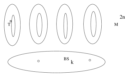
Figure 1: Completely integrable system

There is a couple of equivalent conditions for both of these cases: for a real polarization, for any two vector fields

$$\partial_{1},\partial_{2}\in F\subset T^{\mathbb{C}}M$$ (1.14)

the commutator

$$[\partial_{1},\partial_{2}]\in F\subset T^{\mathbb{C}}M$$ (1.15)

i.e. vector fields from our real distribution form a Lie subalgebra. (Otherwise their commutators form a quadratic form on $F$ with coefficients in $T^{\mathbb{C}}M/F$ just like the second quadratic form in the standard differential geometry of a surface in $\mathbb{R}^{3}$ ).

For the complex case we have to add the equality of the same nature

$$[I\partial_{1},I\partial_{2}]=[\partial_{1},\partial_{2}]+I[I\partial_{1},\partial_{2}]+I[\partial_{1},I\partial_{2}]$$ (1.16)

where we consider $I$ as a section of $EndTM$ with

$$I^{2}=-1$$ (1.17)

$$\omega(\partial_{1},I\partial_{2})=-\omega(I\partial_{1},\partial_{2})$$

$$\omega(\partial_{1},I\partial_{2})>0.$$

These cases are lying in different domains of mathematics: the real polarizations are contained in Symplectic Geometry and the complex polarization belongs to Algebraic Geometry. A quantization is perfect if it admits both of these polarizations. So the perfect quantization belongs to the union of Algebraic and Symplectic Geometries.

1.2 The real polarization.(Symplectic Geometry)

Recall that a subcycle $T\subset M$ is Lagrangian if it is a middle dimensional subcycle such that

$$\omega|_{T}=0.$$ (1.18)

Thus the restriction of the pair $(L,\nabla)|_{T}$ is the trivial line bundle with a flat connection

$$F_{\nabla}|_{T}=2\pi i\omega|_{T}=0.$$ (1.19)

Recall that a gauge class of a flat connection is given by a character of the fundamental group of $T$

$$\chi\colon\pi_{1}(T)\to U(1).$$ (1.20)

Definition 1

A Lagrangian cycle $T$ is Bohr-Sommerfeld if $\chi=1$, that is, if there exists a covariant constant section of $(L,\nabla)|_{T}$.

To kill a character, we need $rkH_{1}(T,\mathbb{Z})$ conditions so we may expect that in a family of Lagrangian cycles the subfamily of Bohr-Sommerfeld cycles has this codimension. Moreover, it was shown that in any small Darboux-Weinstein neighborhood of a smooth Bohr-Sommerfeld cycle $T$ every other Bohr-Sommerfeld cycle $T^{\prime}$ intersects $T$.

For example, our real polarization (1.13) defines a family of Lagrangian cycles parameterized by a space $B$ of dimension $n=1/2\dim M$. But a general fiber of any real polarization fibration $\pi$ (1.13) is a n-dimensional torus, that is

$$rkH_{1}(T^{n})=n=dimB.$$

Thus the set of Bohr-Sommerfeld fibers is discrete and if $B$ is compact it forms a finite set $BS\subset B$ of Bohr-Sommerfeld fibers of $\pi$.

Then the Hilbert space of wave functions is given as the direct sum of lines

$$Q_{F}(M)=\mathcal{H}_{\pi}=\oplus_{b\in BS\subset B}\mathbb{C}\cdot s_{b}$$ (1.21)

where $s_{b}$ is a covariant constant section of $(L,\nabla)|_{\pi^{-1}(b)}$).

Recall that every covariant constant section is defined up to $U(1)$-scaling, so we can define naturally an Hermitian scalar product on this space.

We can extend the notion of Bohr-Sommerfeld Lagrangian cycles:

Definition 2

A Lagrangian cycle $T$ is Bohr-Sommerfeld of level $k$ (or $BS_{k}$ - cycle) if $\chi^{k}=1$, that is, if there exists a covariant constant section of $(L^{k},\nabla_{k})|_{T}$, where $\nabla_{k}$ is the connection generated by $\nabla$ on the tensor power $L^{k}$ of the line bundle $L$.

Reasoning the same way as before, we can prove that the subset $BS_{k}\subset B$ is finite and that the Hilbert space of wave functions of level $k$ is given by the direct sum of lines

$$Q_{F}^{k}(M)=\mathcal{H}_{\pi}^{k}=\oplus_{b\in BS_{k}\subset B}\mathbb{C}\cdot s_{b}$$ (1.22)

where $s_{b}$ is a covariant constant section of $(L^{k},\nabla_{k})|_{\pi^{-1}(b)}$).

But we are quantizing a classical dynamical system $(M,\omega)$! So the result does not have to depend on additional data like $(L,\nabla,\pi,I)$ and so on.

In our construction the wave space $\mathcal{H}_{\pi}$ depends on a gauge class of a connection $\nabla$ only and this class is given by the curvature form if $M$ is simply connected (see [AB]). (Recall that in non-simple connected case we have to fix additionally a point of the ”jacobian” $H^{1}(M,\mathbb{R})/H^{1}(M,\mathbb{Z})$ of $M$ (see below).

In any case our wave function spaces depend up to a shift of characters on the curvature tensor which is $\omega$ and on a choice of a real polarization $\pi$.

Figure 2: twice integrable system

But the most important thing is that the projectivization of the wave functions space doesn’t depend on a real polarization $\pi$ too. For any other Lagrangian fibration $\pi^{\prime}\colon M\to B^{\prime}$, Kostant defined the canonical (up to constant ) pairing between $\mathcal{H}_{\pi}$ and $\mathcal{H}_{\pi^{\prime}}$ (see for example [JW2]). So we get the identification

$$\mathbb{P}\mathcal{H}_{\pi}=\mathbb{P}\mathcal{H}_{\pi^{\prime}}$$ (1.23)

of projective spaces.

Thus $\mathcal{H}_{\pi}$ is the wave space of a quantization of $(M,\omega)$ and of nothing else.

1.3 Kahler quantization. (Algebraic Geometry)

In this case we have a quadruple $(M,\omega,\nabla,I)$ where a complex structure $I$ is compatible with $\omega$. Thus the pair $(\omega,I)$ defines a Kahler metric with the Kahler form $\omega$. Moreover, $\omega$ is of Hodge type (1,1). Thus the connection $\nabla$ on $L$ has the curvature form of type (1,1) and defines a holomorphic structure on $L$ (see for, example, [GH]). As Kodaira (1958) proved, a Kahler metric with integer cohomology class $[\omega]\in H^{2}(M,\mathbb{Z})$ of the Kahler form is a Hodge metric, hence $M_{I}$ is a projective algebraic variety and $L=\mathcal{O}_{M}(1)$ is the class of hyperplane section of $M_{I}$.

So, the complex polarizations bring us to Algebraic Geometry!

Naturally, the wave function space

$$Q_{F}(M)=\mathcal{H}_{I}=H^{0}(M_{I},L)$$ (1.24)

is the space of holomorphic sections of the polarization $L$ and the projectivization $\mathbb{P}H^{0}(M_{I},L)$ is the classical complete linear system on $M_{I}$.

The Hermitian structure on $L$ gives an Hermitian structure on $H^{0}(M_{I},L)$ and provides the identification

$$\mathcal{H}_{I}=H^{0}(M_{I},L)=H^{0}(M_{I},L)^{*}$$ (1.25)

with changing of the complex structure to the complex conjugate.

The standard construction of the Algebraic Geometry gives the following map

$$\phi\colon M_{I}\to\mathbb{P}H^{0}(M_{I},L)^{*},$$ (1.26)

that is, under the previous identification

$$\overline{\phi}\colon M_{I}\to\mathbb{P}H^{0}(M_{I},L).$$ (1.27)

Images of points of $M_{I}$ are called coherent states. A priori such image is defined up to a transformation from $PGL(\mathbb{P}H^{0}(M_{I},L))$. But its every stable orbit contains unique unitary orbit preserving our form $\omega$. If our form $\omega$ is the restriction of the Fubini-Study form from $\mathbb{P}H^{0}(M_{I},L)$, then we can switch on to Geometric Invariant Theory and reduce the theory of coherent states to it. So in algebraic geometrical set up we can assume that our form is a restriction of the Fubini-Study form. In the general case we have to be more careful and to add so called J.Rawnsley $\varepsilon$-function of (see [R]).

Of course we lose the Dirac correspondence and have to use the Berezin-Toeplitz quantization rules (see for example [R]). Thus we introduce the level parameter $k\in\mathbb{Z}^{+}$. The space of wave function of level $k$ is the space of holomorphic sections

$$\mathcal{H}_{I}^{k}=H^{0}(M_{I},L^{k}).$$ (1.28)

The Dirac correspondence can be restored in the quasi classical limit $k\to\infty$ or $1/k\to 0$. So, our complex polarization becomes a polarization in algebraic geometrical sence. Recall that if $k$ is large enough, then $\overline{\phi}$ (1.27) is an embedding and the dimension of the corresponding projective space is given by the Riemann-Roch formula as a pure topological invariant.

So, every underlying symplectic manifold $(M,\omega)$ of a polarized algebraic variety $M_{I},\mathcal{O}(1)$ with a natural complex polarization $\mathcal{O}(1)$ gives the collection of wave functions spaces $H^{0}(M_{I},L^{k})=H^{0}(M_{I},\mathcal{O}(k))$

But the quantization set up disturbs the Algebraic Geometry Peace. The main question is:

do these spaces appear as a result of a successful quantization procedure of a classical system given by the underlying symplectic manifold $(M,\omega)$?

That is,

is the projectivization of this space independent on the complex structure $I$ ?

(In physical symbols, $\frac{\partial\mathbb{P}H^{0}(M_{I},L)}{\partial I}=0$ .)

Mathematically correct question is the following: let $\mathcal{M}$ be the moduli space of such complex structures, that is, the moduli space of polarized (in the algebraic geometryical sense) varieties and

$$p\colon V_{k}\to\mathcal{M},\quad p^{-1}(M_{I})=H^{0}(M_{I},L^{k})$$ (1.29)

- a vector bundle of holomorphic sections of polarization line bundles. Note that by the Kodaira vanishing theorem it is a vector bundle indeed! Then there exists a holomorphic projective flat connection on $V$.

Existence of such connection constraints the topology type of the vector bundle: if a vector bundle $V$ admits a projective flat connection, then

$$c_{t}(V)=(1-c\cdot t)^{rkV}.$$ (1.30)

In particular,

$$c_{1}(V)=rkV\cdot c,\quad c\in H^{2}(\mathcal{M},\mathbb{Z}).$$ (1.31)

This is very strong topological constraint!

Thus problems of new type are given inside of Algebraic Geometry:

When a pair $M_{I},\mathcal{O}(1)$ of an algebraic variety with a polarization is a result of a quantization procedure for the underlying symplectic manifold ?

Before considering the simplest example when $\dim M=2$ we give some general remarks:

1. of course our vector bundles $V_{k}$ (1.29) are holomorphic but the required projective flat connection could be non holomorphic;

2. so, it is quite reasonable to construct may be not holomorphic projective Hermitian connection;

3. in all classical examples holomorphic projective flat connections are Hermitian by the construction;

4. but in the last non-abelian case (which is of the main interest here) this fact isn’t known up to now;

5. if such new connection exists automatically we get a Higgs field on every vector bundle (1.29) on moduli spaces of complex structures.

6. In the physical set up it may be that we do not obtain vector bundles (1.29) but have the collection of projective bundles which aren’t projectivizations of vector bundles;

7. even in the infinite dimensional case (when Hilbert vector bundles are always trivial) the projective bundles can be non trivial and are given by a cohomology class from $H^{3}(\mathcal{M},\mathbb{Z})$. This Brauer group gives us non trivial analog of Atiyah’s K-functor.

In the conformal field theory context this connection always has to be holomorphic but we do not have space and time to discuss it here.

Because of the time-space problem this very interesting subject is out of our considerations here.

1.4 Extended Kodaira-Spencer theory

The theory of deformations of complex structures was developed by Kodaira and Spencer many years ago. Trying ”theoretically” to solve the problem of successful Kahler quantization we have to lift this theory to the problem of holomorphic deformations of a triple $(I,L_{I},(s)_{0})$, where $I$ is an integrable complex structure, $L_{I}$ is our holomorphic line bundle and $s\in H^{0}(L_{I})$ is zero divisor of a holomorphic section of this line bundle. The best reference for such lifting is Welters paper [W]. Recall that the holomorphic structure of $L_{I}$ codes the connection $\nabla$ from the quadruple $(1.7)$ by the decomposition

$$\nabla=\nabla^{1,0}+\nabla^{0,1}$$ (1.32)

where

$$\nabla^{1,0}=1/2\cdot(1-iI)\nabla,\quad\nabla^{0,1}=1/2\cdot(1+iI)\nabla.$$ (1.33)

Our history starts with an infinitesimal deformation of the complex structure $\dot{I}$. Since it is an anti involution $I^{2}=-1$ we have the equality

$$\dot{I}I+I\dot{I}=0$$ (1.34)

and one can consider $\dot{I}$ as a projection of $-i$ eigenspace of $I$ to the $+i$-eigenspace. That is

$$\dot{I}\in\Omega^{0,1}(M_{I},T^{1,0})$$ (1.35)

(just as usual Beltrami differential).

Linearization of the integrability condition (1.16) gives us

$$(\overline{\partial}\dot{I})^{2,0}=0,$$ (1.36)

that is, the (0, 2)-component of this tensor is trivial.

Suppose that we have the following list of properties.

1. Our polarization $L$ is a rational part of the canonical class $K$ of $M_{I}$. That is

   $$-[K]=n[c_{1}(L)].$$ (1.37)

2. Further on we suppose that the Levi-Civita connection of the Kahler metric $\omega(\quad,I\quad)$ (1.17) on $K$ is proportional to the unitary connection on $L$.

3. We consider a sufficiently large level $k$ such that

   $$i>o\implies H^{i}(M_{I},\mathcal{O}(k\cdot c_{1}(L)+1/2K))=0.$$ (1.38)

   (For example, $M_{I}$ is a Fano-variety of index $n$ and $L=\mathcal{O}(k)$).

4. Then we have the symplectic Kahler form

   $$(k+n/2)\omega.$$ (1.39)

From this it is easy to see (for example, by local representation of our tensor) that there exists a section

$$W_{0}\in\Gamma^{\infty}(S^{2}T^{1,0}M_{I})\in(S^{2})^{2,0}$$ (1.40)

where $S^{2}$ is the second symmetrical power of the holomorphic tangent bundle such that the convolution of this tensor with our symplectic form gives us $\dot{I}$:

$$W_{0}*(k+n/2)\omega=\dot{I}.$$ (1.41)

(Recall that $\omega$ is of a type $(1.1)$ with respect to the complex structure $I$.)

To see this very important tensor we have to represent tensors as homomorphisms of tensors vector bundles! By this notation we emphasize that this construction is due to Welters [W]. So our symplectic form

$$(k+n/2)\omega\colon T^{1,0}\oplus T^{0,1}\to\Omega^{1,0}\oplus\Omega^{0,1}$$ (1.42)

is of the Hodge type $(1,1)$ and it means that

$$\omega(T^{1,0})\in\Omega^{0,1}\text{ and }\omega(T^{0,1})\in\Omega^{1,0}.$$ (1.43)

On the other hand,

$$\dot{I}\colon T^{0,1}\to T^{1,0}.$$ (1.44)

Thus the composition of these homomorphisms

$$\dot{I}\circ\frac{1}{k+n/2}\omega^{-1}=W\colon\Omega^{1,0}\to T^{1,0}$$ (1.45)

is the very one symmetric tensor.

Now consider the cup product map

$$H^{0}(M_{I},T^{1,0})\otimes H^{1}(M_{I},\Omega^{0,1})\to H^{1}(M_{I},\mathcal{O})$$ (1.46)

and the restriction of it to $H^{0}(M_{I},T^{1,0})\otimes[(k+n/2)\omega]$:

$$[(k+n/2)\omega]\colon H^{0}(M_{I},T^{1,0})\to H^{1}(M_{I},\mathcal{O}).$$ (1.47)

Suppose that this in an isomorphism. For example

$$H^{0}(M_{I},T^{1,0})=H^{1}(M_{I},\mathcal{O})=0$$ (1.48)

or $M_{I}$ is a polarized abelian variety.

In this case our holomorphic line bundle $L_{I}$ can’t be deformed continuously under deformation of the complex structure. So we have to investigat deformations of holomorphic sections only.

Having such symmetric form and following Nigel Hitchin let us infinitesimally deform a section $s\in H^{0}(M_{I},L_{I})$ to a $\dot{I}$-holomorphic section. Differentiating along a ”time” $t$ the condition $(1+iI_{t})\nabla s_{t}=0$ we get the equality

$$i\dot{I}\nabla^{1,0}s=\nabla^{0,1}a$$ (1.49)

where $-a$ is a section of $L$. Such section depends linearly on $s$ and $\dot{I}$ and defines a connection on the bundle $V$ (1.29). The main observation of the extended Kodaira-Spencer theory is the fact that this equation admits a cohomological interpretation. Namely LHS and RHS of (1.49) are results of applying first order differential operators on $L$. So now we have to consider the vector bundle $D^{1}(L_{I})$ of holomorphic differential operators on $L_{I}$ applied to a holomorphic section in LHS and to the potential of a connection.

Let the exact sequence

$$0\to\Omega^{1,0}\otimes L\to J^{1}(L)\to L\to 0$$ (1.50)

be the extension defining 1-jet bundle of our line bundle $L$. By the Atiyah (see [A2]) theorem, the cocycle of this extension is

$$[c_{1}(L)]=[\omega]\in H^{1}(M_{I},\Omega^{1,0}).$$ (1.51)

Now

$$D^{1}(L)=Hom(J^{1}(L),L)$$ (1.52)

is the bundle of the sheaf of germs of differential operators on $L$ of order $\leq 1$. So this sheaf is the extension

$$0\to\mathcal{O}\to D^{1}(L)\to T^{1,0}\to 0$$ (1.53)

(given by the class $-[\omega]$).

The long exact cohomology sequence of this exact triple decays in two parts

$$0\to H^{0}(M_{I},\mathcal{O})\to H^{0}(M_{I},D^{1}(L))\to 0$$ (1.54)

and

$$0\to H^{1}(M_{I},D^{1}(L))\to H^{1}(M_{I},T^{1,0})\to H^{2}(M_{I},\mathcal{O})\dots$$ (1.55)

because they are divided by the homomorphism (1.44). The first exact sequence states that an every globally defined first order holomorphic operator on $L$ is a multiplication by a constant and the second states that the symbol map $H^{1}(M_{I},D^{1}(L))\to H^{1}(M_{I},T^{1,0})$ is a monomorphism.

Now for a holomorphic section $s\in H^{0}(M_{I},L_{I})$ the valuation morphism

$$d_{s}\colon D^{1}(L)\to L,\quad d_{s}(D)=Ds,$$ (1.56)

gives the complex

$$0\to D^{1}(L)\to L\to 0$$ (1.57)

which hypercohomology $H_{h}^{1}(d_{s})$ defines linear infinitesimal deformations of a triple $(\dot{I},L_{I},s)$.

Each class of such hypercohomology can be done as a pair

$$(\{\dot{s}_{i}\},\{\alpha_{i,j}\})\in C^{0}(\mathcal{U},L)\oplus C^{1}(\mathcal{U},D^{1}(L))$$ (1.58)

where $\mathcal{U}$ is a Cech covering. Indeed it is a 1-cocycle of the total complex, associated with the double complex

$$\pm d_{s}\colon C^{i}(\mathcal{U},D^{1}(L))\to C^{i}(\mathcal{U},L).$$ (1.59)

The spectral sequence of hypercohomology (of a double complex) yields the exact sequence

$$H^{0}(M_{I},D^{1}(L))=\mathbb{C}\to H^{0}(L_{I})\to H_{h}^{1}(d_{s})\to H^{1}(D^{1}(L))\to H^{1}(L_{I})$$ (1.60)

corresponding to the pairs (1.56).

On the other hand, $d_{s}$-complex (1.57) defines the exact quadruple

$$0\to ker_{s}\to D^{1}(L)\to L\to coker_{s}\to 0$$ (1.61)

and the second spectral sequence gives

$$0\to H^{1}(ker)\to H_{h}^{1}(d_{s})\to H^{0}(coker)\to H^{2}(ker).$$ (1.62)

It is easy to see (this observation due to Welters [W]) that the support of the sheaf $coker_{s}$ can be very small:

$$SuppF=Sing(s)_{0}$$ (1.63)

-the singularity locus of the zero-divisor of a section $s$. In particular, if a zero divisor is smooth (this is a general case) then $F=0$ and the exact quadruple (1.60) is in fact a triple.

Now let us return to our main equation (1.49). The RHS admits a solution if the

$$(\overline{\partial}LHS)^{0,2}=0$$ (1.64)

(by the Dolbeault lemma). So we have to compute this RHS Hodge type. But by ( 1.41 ) it is easy to see that

$$(\overline{\partial}(i\dot{I}\nabla^{1,0}))^{0,2}=0.$$ (1.65)

Here we are using

$$i\dot{I}\nabla^{1,0}\in\Omega^{0,1}(M_{I},D^{1}(L))$$ (1.66)

and the infinitesimal integrability condition (1.34). Now we have the interpretations of $i\dot{I}\nabla^{1,0}$ and $-a$ from (1.49) as (0, 1) - forms with coefficients in $D^{1}(L)$ and we have the complex

$$C^{i}=\Omega^{0,i}(M_{I},D^{1}(L))\oplus\Omega^{0,i-1}(M_{I},L_{I})$$ (1.67)

with the differential

$$d(s)(D,a)=(\overline{\partial}D,\overline{\partial}a+(-1)^{i-1}Ds)$$ (1.68)

Now

$$\overline{\partial}s=0\implies d(s)^{2}=0$$ (1.69)

and our pair

$$(i\dot{I}\nabla^{1,0},-a)\in C^{1}.$$ (1.70)

Moreover, equations (1.65) and (1.49) give

$$d(s)(i\dot{I}\nabla^{1,0},-a)=0.$$ (1.71)

Thus, every solution to (1.49) defines a hypercohomology class in $H_{h}^{1}(d_{s})$!

Now suppose we can lift every pair

$$(\dot{I},s)\in\Omega^{0,1}(M_{I},T^{1,0})\oplus H^{0}(M_{I},L_{I})$$ (1.72)

to a cocycle from $H_{h}^{1}(d_{s})$ such that the natural ”symbol” map

$$\sigma\colon H_{h}^{1}(d_{s})\to H^{1}(M_{I},T^{1,0})$$ (1.73)

sends our pair to the cohomology class $[\dot{I}]\in H^{1}(M_{I},T^{1,0})$. That is there exists a map

$$A\colon\Omega^{0,1}(M_{I},T^{1,0})\oplus H^{0}(M_{I},L_{I})\to H_{h}^{1}(d_{s})$$ (1.74)

such that the composition $\sigma A$ is the map to the cohomology class. Then such map defines a projective connection on the vector bundle of holomorphic sections (1.29).

Indeed, we can presents a hypercohomology class as a pair (1.58)

$$(D,s^{\prime})\in\Omega^{0,1}(M_{I},D^{1}(L))\oplus\Omega^{0,0}(M_{I},L_{I}).$$ (1.75)

But now the symbols of operators $-i\sigma(D)$ and $i\dot{I}\nabla^{1,0}$ are cohomological and, therefore the corresponding operators are cohomological in $\Omega^{0,1}(M_{I},D^{1}(L))$ because map to symbols is a monomorphism (1.55). Thus there exists a global operator $\mathcal{D}\Omega^{0}(M_{I},D^{1}(L))$ such that

$$D-i\dot{I}\nabla^{1,0}=\overline{\partial}\mathcal{D}.$$ (1.76)

Since $(D,s^{\prime})$ is a cocycle ($d(s)(D,s^{\prime})=0$, (see (1.71)) one gets

$$Ds+\overline{\partial}s^{\prime}=i\dot{I}\nabla^{1,0}s+\overline{\partial}(\mathcal{D}s+s^{\prime}).$$ (1.77)

Thus

$$-a=\mathcal{D}s+s^{\prime}$$ (1.78)

is a solution for (1.49).

Now for two such solutions hypercocycles $(i\dot{I}\nabla^{1,0},a_{1})$ and $(i\dot{I}\nabla^{1,0},a_{2})$ are cohomological and the hypercocycle

$$(0,a_{1}-a_{2})=d(s)\mathcal{D}^{\prime}.$$ (1.79)

But from the definition of the complex (1.59) we have

$$\overline{\partial}\mathcal{D}^{\prime}=0\implies a_{1}-a_{2}=\lambda s$$ (1.80)

since every first order holomorphic operator is the multiplication by a constant. Geometrically this means that we get a holomorphic connection on the projectivization of our vector bundle.

Thus our last task is to construct the lifting $A$ (1.74). But there is a canonical way to associate such lifting with a holomorphic symmetrical tensor $W$ (1.40).

Consider the sheaf $D^{2}(L)$ of second order holomorphic operators given by the standart extension

$$0\to D^{1}(L)\to D^{2}(L)\to S^{2}(T^{1,0})\to 0.$$ (1.81)

Evaluating differential operators on a given section $s\in H^{0}(M_{I},L_{I})$ we get two homomorphisms

$$d_{s}\colon D^{1}(L)\to L$$ (1.82)

$$d^{\prime}_{s}\colon D^{2}(L)\to L$$

giving two complexes: our complex (1.57) and its analog

$$0\to D^{2}(L)\to L\to 0.$$ (1.83)

Considering the ”trivial” third complex

$$0\to S^{2}(T^{1,0})\to 0\to 0$$ (1.84)

we get the homomorphism of the vertical triples to the triple

$$0\to L\to L\to 0\to 0$$

and the exact triple of these complexes. The corresponding exact sequence of hypercohomology has the form

$$0\to H_{h}^{0}(d_{s})\to H_{h}^{0}(d^{\prime}_{s})\to$$ (1.85)

$$\to H^{0}(M_{I},S^{2}(T^{1,0}))\to H_{h}^{1}(d_{s})\to H_{h}^{1}(d^{\prime}_{s})\to\dots$$

and every holomorphic quadratic form on the tangent bundle defines a 1-hypercohomology class (which may be zero). Of course our required map depends on a choice of a section $s$, so we denote this map by the symbol

$$\phi_{s}\colon H^{0}(M_{I},S^{2}(T^{1,0}))\to H_{h}^{1}(d_{s}).$$ (1.86)

The composition of this map with the forgetful homomorphism $\sigma$ (1.73) gives the homomorphism

$$\mu_{L}\colon H^{0}(M_{I},S^{2}(T^{1,0}))\to H^{1}(M_{I},T^{1,0})$$ (1.87)

which doesn’t depend on the choice of $s$. More precisely

$$\mu_{L}(W_{0})=-W*[c_{1}(L)]+\mu_{\mathcal{O}}$$ (1.88)

It is quite natural to call it the ”cohomological heat equation”. For example for polarized abelian varieties the map $\mu_{\mathcal{O}}=0$. Moreover, all extensions $D^{n}(\mathcal{O})$ are trivial hence all coboundary homomorphisms are trivial.

In particular, from this equality and (1.41) we can see that

$$\mu_{\mathcal{O}}(W_{0})=-W_{0}*1/2K$$ (1.89)

because we can say more about sheaves of differential operators on the trivial line bundle. Namely the extension class for all jet-bundles is equal to

$$1/2[K_{M_{I}}]\in\Omega^{1,1}.$$ (1.90)

From this it is easy to see that

$$\mu_{L}(W_{0})=-W_{0}*([c_{1}(L)]+1/2[K_{M_{I}}])$$ (1.91)

where $K_{M_{I}}$ is the canonical class of $M_{I}$ and the cohomology class $[K_{M_{I}}]$ depends on $\omega$ only (and not on the choice of an admissible complex structure).

Of course we can get more precise formula using representatives of classes by forms and using the Levi-Civita connections for tensor bundles (see [H1])

So the extended Kodaira-Spencer theory gives us (canonically) a holomorphic projective connection on the vector bundles (1.29) but of course to compute a curvature of one we have to present it as a Dolbeault or Cech class.

An existence of Welters tensor $W_{0}$ (1.40) gives strong geometrical constraints. In particular $M_{I}$ can’t be a variety of general type. More precisely the canonical class $K$ of $M_{I}$ can’t be positive.

1.5 Faithful functors

Suppose our $M_{I}$ which we consider as a point $I$ of the moduli space $\mathcal{M}$ of all its deformation defines a new polarized algebraic variety $M^{\prime}_{I^{\prime}}$ which also we consider as a point $I^{\prime}$ of the moduli space $\mathcal{M}^{\prime}$ such a way, that we can reconstruct $M_{I}$ (from the geometry of $M^{\prime}_{I^{\prime}}$). Geometrically, mapping $M_{I}$ to $M^{\prime}_{I^{\prime}}$ defines a holomorphic embedding of moduli spaces

$$J\colon\mathcal{M}\to\mathcal{M}^{\prime},$$ (1.92)

and $J(I)=I^{\prime}$. If a morphism of polarized varities from $\mathcal{M}$ induces a morphism of corresponding varieties from $\mathcal{M}^{\prime}$ then the map $M_{I}\to M^{\prime}_{I^{\prime}}$ is called a faithful functor. From geometrical point of view these geometrical images are undistinguishable in spite of the fact that these varieties can have different dimensions and so on. An algebraic geometer is skillful enough if he can recognize such geometrically undistinguishable varieties of different dimensions and different shapes.

For example, a smooth intersection

$$X=Q_{1}\cap Q_{2}\subset\mathbb{P}^{5}$$ (1.93)

of two quadrics in five dimensional projective space is geometrically equivalent to an algebraic curve $\Sigma_{I}$ of genus 2. To reconstruct $\Sigma_{I}$ from $X$ it is enough to remark that

1. By the Lefshetz theorem $X$ is simply connected;

2. $\mathcal{O}_{X}(-2)=K_{X}$ - the canonical class of $X$. Hence the embedding of $X$ into $\mathbb{P}^{5}$ is canonical.

3. The space of all quadrics in $\mathbb{P}^{5}$ through $X$ is a pencil

   $$|2H-X|=\mathbb{P}^{1}$$ (1.94)

   that is parameterized by the projective line.

4. The subset of singular quadrics in this pencil is six different points

   $$W=p_{1}\cup...\cup p_{6}\subset\mathbb{P}^{1}.$$ (1.95)

5. The double cover

   $$\phi\colon\Sigma_{I}\to\mathbb{P}^{1}$$ (1.96)

   with ramification in these six points $W$ is the required curve $\Sigma_{I}$ of genus 2.

Note that the previous double cover is given by the canonical linear system of $\Sigma_{I}$. Now a simple exercise in linear algebra shows that there exists just one pencil of quadrics in $\mathbb{P}^{5}$ up to a linear transformation with the subset of singular quadrics which is equal to the ramification locus of the double cover.

If $M_{I}\to M^{\prime}_{I^{\prime}}$ is a faithful functor and geometries of both varietes are undistinguishable it is quite reasonable to consider a quantization of $\mathcal{M}^{\prime}$ as a quantization of $\mathcal{M}$, that is, to say

$$Q(M_{I})=Q(M^{\prime}_{I^{\prime}})$$ (1.97)

and so on … We will say that such quantization is successful if the quantization of $\mathcal{M}$ is successful, that is, corresponding vector bundles (1.29) on $\mathcal{M}^{\prime}$ admit projective flat holomorphic connections.

1.6 Perfect quantization

Suppose our algebraic variety $(M_{I},\mathcal{O}(1))$ with a Hodge form $\omega$ admits as a symplectic manifold a real polarization that is a Lagrangian fibration:

$$\pi\colon M\to B,\quad\pi^{-1}(b_{gen})=T^{n}$$ (1.98)

that is the generic fiber is a Lagrangian torus of dimension $n=1/2dimM$;

Again we may suppose that the subset $BS_{k}\subset B$ is finite and the Hilbert space of wave functions of level $k$ is given by the direct sum of lines

$$Q_{F}^{k}(M)=\mathcal{H}_{\pi}^{k}=\oplus_{b\in BS_{k}\subset B}\mathbb{C}\cdot s_{b}$$ (1.99)

where $s_{b}$ is a covariant constant section of $(L^{k},\nabla_{k})|_{\pi^{-1}(b)}$).

Suppose we can construct a natural isomorphism

$$\mathbb{P}Q_{F}^{k}(M)=\mathbb{P}H^{0}(M_{I},\mathcal{O}(k)).$$ (1.100)

Then we have a perfect quantization providing a lot of beautiful and very important properties.

1. First of all, both kinds of quantization are successful : indeed, the LHS of the equality (1.100) doesn’t depend on a complex polarization at all. On the other hand, RHS doesn’t depend on a real polarization.

2. LHS of the equality is decomposed into a sum of lines so the RHS as a space of sections admits a special basis (may be after fixing some additional structure like so called theta - structure for abelian varieties [Mum]).

3. A basis of such type is called the Bohr-Sommerfeld basis.

4. Such situation can be called perfect quantization.

Moreover, the first example of a perfect quantization is given by the classical theory of theta-functions.

Obviously it is not the simplest example. The simplest example is the following: consider the standard two sphere $S^{2}$ realized as the complex Riemann sphere with the standard $U(1)=S^{1}$-action (rotations around North and South Poles). Now $U(1)$-invariant symplectic form $\omega$ of volume 1 gives the phase space of the classical mechanical system $S^{2},\omega$. To quantize this one we have to fix a complex structure, but it is unique and the real polarization

$$\pi\colon S^{2}\to[-1,1]$$ (1.101)

is given by the projection to the rotation axis.

As a prequantization date we get the line bundle $\mathcal{O}(1)$ of degree 1 with the standard $U(1)$-invariant unitary connection $\nabla$. Then the wave function spaces

$$\mathcal{H}^{k}_{I}=H^{0}(\mathcal{O}(k))$$ (1.102)

and $U(1)$- action on this space defines the special eigenbasis of Fourier polynomials. Fourier monomials are in 1-1 correspondence with Bohr-Sommerfeld fibers of the projection (1.101) in angle coordinates. Thus in this case we have the perfect quantization.

It is easy to see that in this case all ”good” theoretical conditions as (1.48) are disturbed but the result of quantization is successful.

If we put out the word ”natural” from the statement (1.100) we get the statement about ranks of both wave functions spaces. In this case we say that the quantization is numerically perfect. The geometry behind this numerical coincidence will be described in (2.25) - (2.30) and [T3]. Such rank’s equalities were proved for K3 surfaces cases and many others. But historically first case was the Gelfand-Cetlin system (see [GS2]).

2 Algebraic curves = Riemann surfaces

2.1 Direct approach

Let $\Sigma$ be a compact smooth oriented Riemann surface and $\Sigma_{I}$ be a complex structure on it, thus, one has an algebraic curve of genus $g>1$. Such curves admit the canonical polarization by the cotangent bundle $T^{*}\Sigma_{I}=\mathcal{O}(K)$ where $K$ is the canonical class of $\Sigma_{I}$ (see for example [DSS]). Moreover, if we fix a metric on $\Sigma$ with the conformal class given by the complex structure $I$ then the Levi-Civita connection on the cotangent bundle gives the prequantization data $(T^{*}\Sigma,\nabla_{LC})$. This pair is equivalent to the holomorphic pair $(\Sigma_{I},\mathcal{O}(K))$.

The union of all spaces $H^{0}(\mathcal{O}(kK))$ of holomorphic sections gives the collection of vector bundles

$$p_{k}\colon V_{k}\to\mathcal{M}_{g},\quad p^{-1}(M_{I})=H^{0}(M_{I},\mathcal{O}(kK))$$ (2.1)

on the moduli space $\mathcal{M}_{g}$ of curves of genus $g$. (Recall that $\dim\mathcal{M}_{g}=3g-3$).

In particular, for $k=2$ the vector bundle $V_{2}=T^{*}\mathcal{M}_{g}$ is the cotangent bundle of the moduli space, that is, $V_{2}$ is the bundle with spaces of quadratic differentials as fibers. In particular the canonical class $K_{\mathcal{M}_{g}}$ is the first Chern class of the vector bundle $V_{2}$:

$$c_{1}(V_{2})=K_{\mathcal{M}_{g}}.$$ (2.2)

Now according to Mumford this canonical class has the decomposition

$$K_{\mathcal{M}_{g}}=13\Theta+\text{boundary divisors $\dots$}$$ (2.3)

where $\Theta$ is the diviser of zero theta constants.

If the vector bundle $V_{2}$ admits a holomorphic projective flat connection then by (1.31) the number 13 has to be divided by $3g-3$. This isn’t the case thus $V_{2}$ doesn’t admit any flat connection and an algebraic curve as a polarized algebraic variety isn’t a result of a successful quantization procedure of the classical dynamical system $(\Sigma,\omega)$ where $\omega$ is the restriction of the Fubini-Study form.

But the history isn’t finished! We can find a ”faithful functor”.

2.2 Jacobians

May be the first faithful functor for algebraic curve is mapping of the curve to the polarized jacobian $(J(\Sigma_{I}),\Theta)$. There exists a lot of constructions but for us it will be very convinient to consider $J(\Sigma_{I})$ as the moduli space of holomophic topological trivial line bundles. Fixing a point $p_{0}\in\Sigma_{I}$ we consider for every other point $p\in\Sigma_{I}$ the topological trivial line bundle $\mathcal{O}(p-p_{0})$, where we consider points as divisors of degree 1. So we get the map

$$a_{p_{0}}\colon\Sigma_{I}\to J(\Sigma_{I}).$$ (2.4)

By the Riemann theorem this map is an embedding (if genus $g>0$) and induces the isomorphism

$$a\colon H_{1}(\Sigma,\mathbb{Z})\to H_{1}(J(\Sigma_{I}),\mathbb{Z}).$$ (2.5)

The moduli space of line bundles is a group (with respect to the tensor product of line bundles). So, we can consider the Pontrjagin map

$$a_{p_{0}}^{g-1}\colon\Sigma_{I}^{[g-1]}\to J(\Sigma_{I})$$ (2.6)

sending a finite set of points $\{p_{1},...,p_{g-1}\}$ to the line bundle

$$\mathcal{O}(p_{1}+...+p_{g-1}-(g-1)p_{0})\in J(\Sigma_{I}).$$ (2.7)

The image of this map is a divisor $\Theta$ (so called theta diviser) and the corresponding line bundle admits only one (up to $\mathbb{C}^{*}$) holomorphic section (with the zero set $\Theta$).

To reconstruct the curve $\Sigma_{I}$ from the pair $(\Theta\subset J(\Sigma_{I}))$ we have to consider the Gauss map

$$G\colon\Theta\to\mathbb{P}T^{*}J(\Sigma_{I})$$ (2.8)

to the projectivization of the cotangent bundle sending non singular point of $\Theta$ to the tangent hyperplane to $\Theta$ at this point. But the cotangent bundle (of a group) is trivial $\mathbb{P}T^{*}J(\Sigma_{I})=\mathbb{P}^{g-1}\times J(\Sigma_{I})$, and the composition of the projection to $\mathbb{P}^{g-1}$ and the Gauss map gives the rational cover

$$G\circ p\colon\Theta\to\mathbb{P}^{g-1}.$$ (2.9)

Now the ramification diviser of this cover is the dual divisor to the canonical embedding of $\Sigma_{I}$ into $(\mathbb{P}^{g-1})^{*}$ (for hyperelliptic curves we use other arguments). By the classical projective duality theory we can reconstruct a curve by its dual divisor. Thus the sending of a curve $\Sigma_{I}\to(J(\Sigma_{I}),\Theta)$ is a faithful functor.

Now using our rule (1.97) we may quantize the polarized variety $(J(\Sigma_{I}),\Theta)$.

The role of wave function spaces now are played by the spaces of holomorphic sections:

$$\mathcal{H}_{I}^{k}=H^{0}(J(\Sigma_{I}),\mathcal{O}(k\Theta)).$$ (2.10)

These spaces are called spaces of theta function of the Riemann surface $\Sigma_{I}$ of level $k$.

This quantization is successful! Corresponding vector bundles on the moduli space admit projective flat connections (see [W]). But the situation is much better than just a successful quantization.

2.3 Algebro geometrical theory of theta functions

.

Consider a principal polarized abelian variety $(A,\Theta)$ of dimension $g$. Then the line bundle $\mathcal{O}(k\Theta)$ admits the finite group $K$ of translations preserving this line bundle. It is easy to see that

$$K=A_{k}\subset A$$ (2.11)

is the subgroup of points of order $k$ in the abelian group $A$. Recall that we have a symplectic form on $K$ given by the wedge product of 1-cycles coupled by the polarization $\Theta$. The decomposition

$$K=K_{+}\times K_{-}$$ (2.12)

by two isotropic subgroups of this group is called theta-structure of level $k$.

The beautiful classical result reproduced by Mumford is the following

1. In the complete linear system $|k\Theta|$ there exists only one divisor $D_{+}$ which is invariant with respect to the subgroup $K_{+}$ - action.

2. Every translation $a\in K_{-}$ defines a divisor $D_{+}+a$ and the rational function $\theta_{a}$ with pole at the divisor $D_{+}$ and zeros at the divisor $D_{+}+a$. This function is called theta function with characteristic $a\in K_{-}$.

3. The space of holomorphic sections

   $$H^{0}(A,\mathcal{O}(k\Theta))=H^{0}(A,\mathcal{O}(D_{+}))=\oplus_{a\in K_{-}}\mathbb{C}\theta_{a}.$$ (2.13)

4. This is the theta functions with characteristics decomposition.

Note, that the cardinalities of our finite abelian groups are given by formulas

$$|K|=k^{2g},\quad|K_{\pm}|=k^{g}.$$ (2.14)

Now it is quite useful to apply the extended Kodaira-Spenser theory to this situation. First of all for every abelian variety

$$H^{0}(A,T)\to H^{2}(A,\mathcal{O})$$ (2.15)

is an isomorphism thus the condition (1.48) holds. Moreover, from cohomology sequence of (1.50) we have

1. an isomorphism

   $$H^{0}(A,S^{2}(T))=H^{1}(A,D^{1}(k\Theta)));$$ (2.16)

2. $$H^{0}(A,\mathcal{O})=H^{0}(A,D^{1}(\mathcal{O}(k\Theta)));$$ (2.17)

3. and from (1.60) we have

   $$0\to H^{0}(A,\mathcal{O}(k\Theta))/\mathbb{C}\cdot s\to H_{h}^{1}(d_{s})\to H^{1}(A,D^{1}(\mathcal{O}(k\Theta)))\to 0;$$ (2.18)

4. so under a deformation of the pair $(A,\mathcal{O}(k\Theta))$ for every section $s$ there exits unique deformation of this section which is defined by the heat equation (see the standard presentation (2.49) below).

2.4 Symplectic-combinatorial theory of theta functions

A principal polarization $\Theta$ on an abelian variety $A$ can be done by some unimodular skew symmetrical integer form

$$\omega\in H^{2}(A,\mathbb{Z})$$ (2.19)

because $A$ is a $2g$-dimensional real torus:

$$\omega\in\wedge^{2}H^{1}(A,\mathbb{Z})=H^{2}(A,\mathbb{Z}).$$ (2.20)

For a jacobian $J(\Sigma)$ this form is induced by the intersection form on 1-cycles on the Riemann surface $\Sigma$.

The theory of unimodular integer skew symmetrical forms predicts that there are two isotropic $\mathbb{Z}$-sublattices in $H^{1}(A,\mathbb{Z})$ such that our form $\omega$ has the standard symplectic shape.

Recall that the underlying smooth manifold of our abelian variety is nothing else but a real torus $T^{2g}$ and the decomposition of $H^{1}(A,\mathbb{Z})$ by two isotropic $\mathbb{Z}$-submodules induces the corresponding decomposition of this torus into two families of Lagrangian subtori

$$T^{2g}=T^{g}_{+}\times T^{g}_{-}.$$ (2.21)

Considering the projection to the second $g$-torus

$$\pi\colon T^{2g}\to T^{g}_{-}$$ (2.22)

we obtain an integrable system that is a real polarization of the torus $T^{2g}=A$.

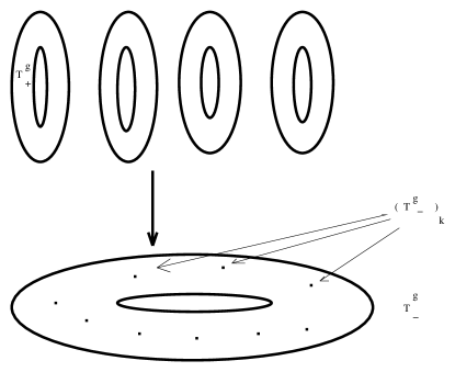
Figure 3: Bohr-Sommerfeld fibers

The direct interpretation of the prequantization line bundle shows that the subset of $k$-Bohr-Sommerfeld fibers

$$BS_{k}=(T^{g}_{-})_{k}\subset T^{g}_{-}$$ (2.23)

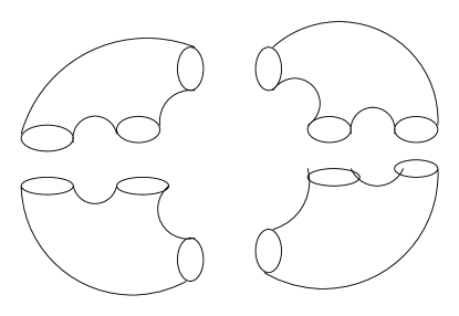
Figure 5: Pairs of pants

is the subgroup of points of order $k$ on our second torus $T^{g}_{-}$ (see Fig.5). So, the wave function space of the Bohr-Sommerfeld quantization is the sum of lines

$$Q_{\pi}^{k}(T^{2g},\omega)=\oplus_{a\in(T^{g}_{-})_{k}}\mathbb{C}\cdot s_{a}$$ (2.24)

where $s_{a}$ are covariant constant sections of restrictions of the prequantization line bundle.

We can see that the results of the Kahler quantization and the Bohr-Sommerfeld quantization give wave function spaces of the same rank so the quantization is numericaly perfect (see the end of subsection 1.5).

This is the first amazing fact in this story. We would like to say couple of words about the geometry behind such coincidence.

Returning to the fibration (2.22) we can construct so called dual fibration

$$\pi^{\prime}\colon(T^{\prime})^{2g}\to T^{g}_{-}$$ (2.25)

changing every torus-fiber $T^{g}_{+}$ by the dual torus $(T^{g}_{+})^{*}$. This dual torus is nothing else but the space of gauge classes of all $U(1)$-flat connections on the trivial line bundle on $T^{g}_{+}$. We have got a priori a new $2g$-torus with new symplectic form $\omega^{\prime}$ of the same type as before.

Now consider any holomorphic line bundle $L$ on our old complex torus $A$ with $U(1)$-connection which curvature form has to be proportional to $\omega$. (Just like our prequantization bundle $\mathcal{O}(k)$). Then for every point $a\in T^{g}_{+}$ the restriction of $L$ to the Lagrangian fiber $\pi^{-1}(a)$ gives a flat line bundle, that is the point of the dual fibers

$$s_{L}\in(T^{g}_{+})^{*}=(\pi^{-1}(a))^{*}.$$ (2.26)

Thus every such line bundle defines a section

$$s_{L}\colon T^{g}_{+}\to(T^{\prime})^{2g},$$ (2.27)

that is a middle dimensional submanifold $s_{L}$ (more precisely $s_{L}(T^{g}_{+})$) in the manifold $(T^{\prime})^{2g}$.

Of course trivial connection defines zero section of the new fibration (2.25) that is we have a middle dimensional submanifold

$$s_{\mathcal{O}(0)}\subset(T^{\prime})^{2g}.$$ (2.28)

Obviously, the intersection set

$$s_{\mathcal{O}(0)}\cap s_{\mathcal{O}(k)}=BS_{k}$$ (2.29)

is the set of Borh-Sommerfeld fibers of level $k$. Moreover, it is easy to see that both our cycles are Lagrangian, oriented and admit positive index intersections only. Thus the number of Bohr-Sommerfeld fibers is given by the intersection index of cohomology classes

$$[s_{\mathcal{O}(0)}]\cdot[s_{\mathcal{O}(k)}]=\#BS_{k}.$$ (2.30)

Now using the first Chern class of the polarization we can easily compute these numbers.

The moral is the following: an abelian variety $A=T^{2g}$ has a symplectic partner $(T^{\prime})^{2g}$ such that coherent sheaves geometry on $A$ can be encoded by the geometry of Lagrangian cycles (or super cycles) on the partner $(T^{\prime})^{2g}$. Usually this partner is called mirror partner. Mirror symmetry now is far developed domain so we can’t dive to this subject (see [CK]). In spite of the coincidence of our previous construction with the Strominger-Yau-Zaslow mirror symmetry construction we would like to stop here discussion of this subject but formally it can be extended along this line (see [T3]).

Of course the dimensional coicidence can be also extended. Moreover there are theta bases in both of wave function spaces. To compare them we have to construct a holomorphic object, namely, a section of the theta bundle of level $k$ using only Bohr-Sommerfeld fiber of the projection $\pi$ (2.22) (see Figure 1).

We will do this using so called coherent state transform or the slightly generalized Segal-Bargmann isomorphism introduced in the context of the quantum theory as a transform from the Hilbert space of square integrable functions on the configuration space to the space of holomorphic functions on the phase space.

Considering zero fiber $T^{g}_{+}$ of the polarization map $\pi$ (2.22) we can interpret our complex torus $A$ as a complexification of this real torus and input our geometrical situation to the situation of the classical coherent state transform.

In the finite dimensional context a configuration space is just $\mathbb{R}^{g}$ as the real part of the phase space $\mathbb{C}^{g}$. The coherent state transform

$$CST_{t}\colon L^{2}(\mathbb{R}^{g},d^{g}x)\to L^{2}(\mathbb{C}^{g},d\mu_{t})\cap\mathcal{H}(\mathbb{C}^{g})$$ (2.31)

is a unitary isomorphism.(Here $d\mu_{t}$ is the Gaussian measure and $\mathcal{H}$ is the space of holomorphic functions.)

For our abelian case we have to replace $\mathbb{R}^{g}$ by $T^{g}=U(1)^{g}$ and $\mathbb{C}^{n}$ by our complex torus $A$. Remark that $T^{g}$ in our case is a special Lagrangian subtorus (see, for example [T4]).

B. C. Hall proposed a generalization of the CST where $\mathbb{R}^{n}$ is replaced by $\operatorname{SU}(2)$ and $\mathbb{C}^{n}$ by $SL(2,\mathbb{C})$ (see [Ha]) and we will use it later for non-abelian case. But here we use this construction for abelian group $U(1)^{g}\subset(\mathbb{C}^{*})^{g}$.

First of all, the decomposition (2.21) induces the decomposition

$$H^{1}(A,\mathbb{Z})=H^{1}(T^{g}_{+},\mathbb{Z})\oplus H^{1}(T^{g}_{-},\mathbb{Z}).$$ (2.32)

Let us fix a basis $(a_{1},\dots,a_{g})$ in the lattice $H^{1}(T^{g}_{+},\mathbb{Z})$ and a basis $(b_{1},\dots,b_{g})$ in the lattice $H^{1}(T^{g}_{-},\mathbb{Z})$ such that the full system $(a_{1},\dots,a_{g},b_{1},\dots,b_{g})$ is a standard basis of 1-homology of $A$. For a complex Riemann surface $\Sigma$ consider the period matrix

$$\Omega=\|\Omega_{ij}\|=Re\Omega+i\cdot Im\Omega$$ (2.33)

as a point of the Siegel space $H$. Let $\vec{x}=(x_{1},\dots,x_{g})\in[0,1]^{g}$ be periodic coordinates on $U(1)^{g}=T^{g}_{+}$. Then we have $U(1)$-invariant Laplacian

$$\Delta^{Im\Omega}=\sum_{i,j=1}^{g}\frac{Im\Omega_{ij}}{2\pi}\frac{\partial^{2}}{\partial x_{i}\partial x_{j}}.$$ (2.34)

The complexification of $T^{g}_{+}$ is $(\mathbb{C}^{*})^{g}$ with coordinates $(e^{2\pi iz_{1}},\dots,e^{2\pi iz_{g}})$ for $\vec{z}=\vec{x}+i\vec{y}$. Then the Haar mesure on $(\mathbb{C}^{*})^{g}$ is $d\vec{x}d\vec{y}$ and we have $U(1)^{g}$-invariant complex Laplacian

$$\Delta^{Im\Omega}_{\mathbb{C}}=\sum_{i,j=1}^{g}\frac{Im\Omega_{ij}}{2\pi}(\frac{\partial^{2}}{\partial x_{i}\partial x_{j}}+\frac{\partial^{2}}{\partial y_{i}\partial y_{j}}).$$ (2.35)

As the first step consider the fundamental solution $\mu_{t}$ at the identity of the heat equation on $(\mathbb{C}^{*})^{g}$

$$4\frac{\partial u}{\partial t}=\Delta^{Im\Omega}_{\mathbb{C}}u$$ (2.36)

and average the measure $\mu_{t}d\vec{x}d\vec{y}$ with respect to the action of $U(1)^{g}$ :

$$\nu_{t}(\vec{z})d\vec{x}d\vec{y}=(\int_{U(1)^{g}}\mu_{t}(\vec{z}+\vec{x})d\vec{x})\quad d\vec{x}d\vec{y}.$$ (2.37)

The explicit formula is

$$\nu_{t}(\vec{z})=(\frac{2}{t})^{g/2}(det(Im\Omega))^{-1/2}e^{\frac{\pi}{2t}\sum_{i,j}(z_{i}-\overline{z_{i}})(Im\Omega)^{-1}_{ij}(z_{j}-\overline{z_{j}})}.$$ (2.38)

Now consider non-self adjoint Laplace operator

$$\Delta^{-i\Omega}=\sum_{i,j=1}^{g}\frac{i}{2\pi}\Omega_{ij}\frac{\partial^{2}}{\partial x_{i}\partial x_{j}}.$$ (2.39)

C. Florentino, J. Mourao and J. Nunes proved in [FMN] the following

Proposition 1

Let $\mathcal{C}$ be the analytic continuation from $U(1)^{g}$ to $(\mathbb{C}^{*})^{g}$. Then the transform

$$C_{t}^{(-i\Omega)}=\mathcal{C}\circ e^{t/2\Delta^{(-i\Omega)}}\colon L^{2}(U(1)^{g},d\vec{x})\to$$ (2.40)

$$\to L^{2}((\mathbb{C}^{*})^{g},d\nu_{t})\cap\mathcal{H}((\mathbb{C}^{*})^{g})$$

is unitary.

So for any function $f\in L^{2}(U(1)^{g},d\vec{x})$ given by its Fourier decomposition

$$f(\vec{x})=\sum_{\vec{n}\in\mathbb{Z}^{g}}a_{n}e^{2\pi i\vec{x}\cdot\vec{n}}$$ (2.41)

we have

$$(C_{t}^{(-i\Omega)}f)(\vec{z})=\sum_{\vec{n}\in\mathbb{Z}^{g}}a_{n}e^{ti\pi\vec{n}\Omega\vec{n}}\cdot e^{2\pi i\vec{x}\cdot\vec{n}}.$$ (2.42)

This function is the analytic continuation to $(\mathbb{C}^{*})^{g}$ of the solution of the complex heat equation

$$2\frac{\partial u}{\partial t}=\Delta^{(-i\Omega)}u$$ (2.43)

on $(\mathbb{C}^{*})^{g}$ with the initial condition given by f.

But the coherent states transform (2.40) can be extended from $L^{2}(U(1)^{g},d\vec{x})$ to the space of distributions $(C^{\infty}(U(1)^{g}))^{\prime}$ given by Fourier series of the form (2.41) such that there exists an integer $N>0$ such that

$$lim_{\vec{n}\cdot\vec{n}\to\infty}\frac{|a_{n}|}{(1+\vec{n}\cdot\vec{n})^{N}}=0.$$ (2.44)

The Laplace operator and its powers act as continuous linear operators on this space of distributions (by duality from the corresponding action on $C^{\infty}(U(1)^{g})$) and define for ($t>0$) the action of the operator $e^{t/2}\Delta^{(-i\Omega)}$ on distributions $f$ of the form (2.41) as

$$e^{t/2}\Delta^{(-i\Omega)}(\sum_{\vec{n}\in\mathbb{Z}^{g}}a_{n}e^{2\pi i\vec{x}\vec{n}})=$$ (2.45)

$$=\sum_{\vec{n}\in\mathbb{Z}^{g}}a_{n}e^{ti\pi\vec{n}\Omega\vec{n}}e^{2\pi i\vec{z}\vec{n}}.$$

In the same paper [FMN] the authors proved the following

Proposition 2

If a series $f\in(C^{\infty}(U(1)^{g}))^{\prime}$ then the RHS of (2.45) defines a holomorphic function on $(\mathbb{C}^{*})^{g}$.

Now we are ready to map every Bohr-Sommerfeld fiber of the projection (2.22) to an analytic function on $(\mathbb{C}^{*})^{g}$. It is enough to do it for zero torus $T^{g}_{+}=U(1)^{g}$ of this projection.

For this let us consider the distribution

$$\theta^{\mathbb{R}}_{0}(x)=\sum_{\vec{n}\in\mathbb{Z}^{g}}e^{2\pi ik\vec{x}\vec{n}}.$$ (2.46)

It is nothing else but the delta-function at the identity of level $k$. Let us apply CST (2.40) to this distribution:

$$C_{1/k}^{(-i\Omega)}(\theta_{k}^{\mathbb{R}})=$$ (2.47)

$$=\sum_{\vec{n}\in\mathbb{Z}^{g}}e^{\pi ik\vec{n}\cdot\Omega/k\vec{n}k}\cdot e^{2\pi ik\vec{n}\vec{z}}.$$

For every $l\in\mathbb{Z}^{g}/k\mathbb{Z}^{g}$ we can start with the function

$$\theta^{\mathbb{R}}_{l}(x)=\sum_{\vec{n}\in\mathbb{Z}^{g}}e^{2\pi i\vec{x}(l+k\vec{n})}$$ (2.48)

to get the analytic function

$$C_{1/k}^{(-i\Omega)}(\theta_{l}^{\mathbb{R}})=\theta_{l}(z,\Omega)=$$ (2.49)

$$=\sum_{\vec{n}\in\mathbb{Z}^{g}}e^{\pi i(l+k\vec{n})\cdot\Omega/k(l+k\vec{n})}\cdot e^{2\pi i(l+k\vec{n})\vec{z}}.$$

Remark that we are substitute our continious positive parameter $t$ coming from heat kernels by its discrete conterpart $1/k$.

We would like to emphasize that in spite of 150 years of development of the classical theory of theta functions this ”comparing quantization” approach was realized first quite recently by C. Florentino, J. Mourao and J. Nunes in [FMN].

What we have to do now is just to compare our holomorphic functions on $(\mathbb{C}^{*})^{g}$ with holomorphic sections of the $\Theta$-line bundle on $A$.

2.5 Abelian holomorphic flat connections

The usual way to define a line bundle $L$ is to consider some finite cover $\{U_{i}\}$ on the base and a collection of transition functions $f_{ij}$ which are regular and regular inversed on $U_{i}\cap U_{j}$. On the intersection $U_{i}\cap U_{j}\cap U_{k}$ we have the cocycle equality

$$f_{ij}\cdot f_{jk}\cdot f_{ki}=1.$$ (2.50)

A collection $f_{ij}$ is equivalent to a collection $f^{\prime}_{ij}$ iff there exists a collection $\{\beta_{i}\}$ of functions, where each $\beta_{i}$ is regular and regular inversed on $U_{i}$ such that

$$f^{\prime}_{ij}=\beta_{i}f_{ij}\beta_{j}^{-1}.$$ (2.51)

The idea is to make these functions (2.51) as simple as possible using this equivalence: for example take all $f^{\prime}_{ij}$ constant.

Starting with any collection of functions (2.50) let us consider the collection of differentials forms

$$\{f_{ij}^{-1}df_{ij}\}\in Z^{1}(\{U_{i}\})$$ (2.52)

Obviously, this cochain is a cocycle from $H^{1}(\Omega)=H^{1,1}$ whose cohomology class

$$c(L)\in H^{1,1}$$ (2.53)

is the first Chern class of $L$.

If this class is zero then the cocycle is trivial and there are matrices of differential forms $h_{i}$ such that

$$f_{ij}^{-1}df_{ij}=h_{i}-h_{j}.$$ (2.54)

Definition 3

A collection of differential forms $h_{i}$ on $U_{i}$ is called flat holomorphic connection of the vector bundle $L$ given by the collection of transition functions $f_{ij}$.

Having such collection we can solve the system of linear equations on $U_{i}$

$$\beta_{i}^{-1}\cdot d\beta_{i}=h_{i}$$ (2.55)

and obtain a new collection of transition functions (2.51). Now using all equations we can see that functions $f^{\prime}_{ij}=\beta_{i}\alpha_{ij}\beta_{j}^{-1}$ are constant, that is

$$df^{\prime}_{i}j=0.$$ (2.56)

If transition functions are constant then this vector bundle is called local system of coefficients and we can trivialize it over any simply connected open set. Thus we have a character of the fundamental group of our base:

$$\rho\colon\pi_{1}\to\mathbb{C}^{*}.$$ (2.57)

For a curve we’ve proved the classical result of Poincare:

Proposition 3

Every $L\in J(\Sigma)$ admits holomorphic flat connection given by a character $\chi\colon\pi_{1}(\Sigma)\to\mathbb{C}^{*}$.

How many characters give the same vector bundle? Just as many as flat connections admitted by this bundle there are. The difference of any two holomorphic connections can be identified over $U_{i}\cap U_{j}$, thus

$$\{h_{i}\}-\{h^{\prime}_{i}\}\in H^{0}(\mathcal{O}_{\Sigma}(K_{\Sigma})).$$ (2.58)

By Serre duality

$$H^{1}(\mathcal{O})^{*}=H^{0}(\mathcal{O}(K_{\Sigma}))$$ (2.59)

is a fiber of the cotangent bundle $T^{*}J(\Sigma)$.

The full space $A$ of all holomorphic flat connections is the space of all characters

$$A=(\mathbb{C}^{*})^{2g},\quad dim_{\mathbb{C}}A=2g$$ (2.60)

Every character defines a holomorphic vector bundle by the standard construction

$$L=U\times\mathbb{C}/(\pi_{1},\rho)$$ (2.61)

where $U$ is the universal cover of our base with the natural action of the fundamental group of a base on $U$ and the $\rho$-action on $\mathbb{C}$ .

Thus we have the forgetful map

$$f\colon A\to J(\Sigma).$$ (2.62)

Every fiber of this map is the set of holomorphic flat connections on a fixed line bundle. Thus the map $f$ sending each character to the corresponding line bundle provides on $A$ the structure of an affine bundle over the cotangent bundle.

So fibers of $f$ are affine spaces over $H^{0}(J(\Sigma),\Omega)$ (but in this case the cotangent bundle is the trivial $g$-dimensional vector bundle). Over every small open set $U_{i}$ our affine bundle admits a section that is can be identified with the restriction of the cotangent bundle. Any descrepance exists only on the intersections $U_{i}\cap U_{j}$. The collection of differences of sections gives a 1-cocycle

$$\varepsilon\in H^{1}(J(\Sigma),\Omega).$$ (2.63)

If this cocycle is trivial, our affine bundle coincides with its vector bundle while non trivial affine bundle is defined by this cocycle uniquely. By the Dolbeault theorem in our case the cocycle $\varepsilon_{A}\in H^{1,1}=H^{2}(J(\Sigma),\mathbb{C})$. Poincare proved that

$$\varepsilon_{A}=[\Theta]=[\omega].$$ (2.64)

To prove this equality we have to use the functional equation for theta functions.

The affine bundle (2.62) admits non holomorphic sections: let $U(1)\subset\mathbb{C}^{*}$ be the subgroup of unit norm numbers. There is a map

$$mod\colon\mathbb{C}^{*}\to U(1),\quad z\to\frac{z}{|z|}.$$ (2.65)

Then we have the subspace

$$U(1)(\mathbb{C}^{*})^{2g}$$ (2.66)

of unitary characters of $\pi_{1}(\Sigma)$ which is a section of the projection $f$ (2.62) of the affine vector bundle $(\mathbb{C}^{*})^{2g}$. It follows immediately from the maximum principle for a compact complex manifold.

So we have the smooth identification

$$J(\Sigma)=U(1)^{2g}.$$ (2.67)

Let $H_{1}(\Sigma,\mathbb{Z})=<a_{1},...,a_{g},b_{1},...,b_{g}>$ be as before (see (2.32)).Such presentation defines very important subspace of the character space, so called abelian Schottky subspace:

$$S^{a}_{g}=(\mathbb{C}^{*})^{g}=\{\chi\in(\mathbb{C}^{*})^{2g}|\chi(a_{i})=1\}.$$ (2.68)

and

$$uS^{a}_{g}=(U(1))^{g}=\{\chi\in U(1)^{2g}|\chi(a_{i})=1\}$$ (2.69)

is abelian unitary Schottky space.

The restrictions of the forgetful map $f$ (2.62) onto this space has the following properties

1. $f\colon S^{a}_{g}=(\mathbb{C}^{*})^{g}\to J(\Sigma)$ is infinite ($\mathbb{Z}^{g}$) cover,

2. $f^{*}(\mathcal{O}(\Theta))$ is trivial, so holomorphic sections = holomorphic functions = theta functions;

3. this line bundle is given by the automorphy factors

   $$e_{a_{i}}(z)=1$$ (2.70)

   $$e_{b_{i}}(z)=e^{-2\pi z_{i}-\pi i\Omega_{ii}}$$

   where $\vec{z}$ are complex coordinates of the universal cover $U$ of $A$ described after formula (2.34), $\Omega$ is the period matrix of $\Sigma$ and so on (see the set up around (2.32) - (2.35)); let $\{u_{i}\}$ be the basis in $U$ dual to $\{a_{i}\}$ and

   $$u_{g+i}=\sum_{1}^{g}\Omega_{ij}u_{i};$$ (2.71)

4. thus using these automorphy factors we see that the space $H^{0}(J(\Sigma),\mathcal{O}(k\Theta))$ is naturaly identifyed with the space of holomorphic functions $\theta$ on $(\mathbb{C}^{*})^{g}$ such that $\theta(z+u_{i})=\theta$ and

   $$\theta(z+u_{g+i})=e^{-2\pi kz_{i}-\pi ik\Omega_{ii}};$$ (2.72)

5. thus any $\theta(z)$ admits the following decomposition

   $$\theta(z)=\sum_{l\in\mathbb{Z}^{g}/k\mathbb{Z}^{g}}\theta_{l}(z,\Omega)$$ (2.73)

   where theta functions with characteristics are functions (2.49).

2.6 Perfect quantization

Summarizing all results and constructions, we have

Theorem 1

Principal polarized abelian varieties (and hence algebraic curves) admit the perfect quantization by theta functions.

In particular, we proved very important fact (which we want to generalize for the non-abelian case):

Proposition 4

The Bohr-Sommefeld wave space (2.24) doesn’t depend on the decomposition (2.21) determining projection $\pi$ (2.22). This decomposition defines a basis in this space only and the result of Bohr-Sommerfeld quantization doesn’t depend on the choice of a real polarization of an ”arithmetical” type (2.22).

Of course this observation is obvious in the set-up of the classical theory of theta functions, but in the set-up of non-abelian theta functions it is giving an important ”independence condition” in CQFT and low dimensional topology.

Let us list the sequence of tasks necessary to get a perfect quantization:

1. a $g$-torus $U(1)^{g}$ with the marked point $0\in U(1)^{g}$ we identify with the zero fiber of the fibration $\pi:A\to T^{g}_{-}$ (2.22) containing zero point;

2. for zero point $0\in U(1)^{g}$ we construct $\delta$-function $\theta_{0}^{\mathbb{R}}$ as the Fourier serie (2.46);

3. using the period matrix $\Omega$ of $A$ we construct CST $C^{(-i\Omega)}_{1/k}$ (2.40) , (2.41);

4. applying this transform to the distribution $\theta_{0}^{\mathbb{R}}$ we get the collection of holomorphic theta functions with characteristics $\{\theta_{l}(z,\Omega)\}$ (2.49) on the complexification $(\mathbb{C}^{*})^{g}$ of $U(1)^{g}$;

5. using the periods matrix $\Omega$ we construct the cover $(\mathbb{C}^{*})^{g}\to A$ and get sections of the line bundle $\mathcal{O}(k\Theta)$ as functions subjecting to automorphity factors conditions (2.70);

6. to check that functions $\{\theta_{l}(z,\Omega)\}$ (2.49) correspond to sections of $\mathcal{O}(k\Theta)$.

This is the end of story for the moduli spaces of topological trivial vector bundles of rank one on algebraic curves=Riemann surfaces. But any curve $\Sigma$ also has the other ”moduli space”, namely the moduli space of topological trivial vector bundles of rank 2. This is a faithful functor too. To implement this theory we have to plug Conformal Field Theory in dimension $D=2$. We will use the previous list of tasks as a pattern of much more sophisticated efforts in this ”non-abelian” case.

Note that $H^{0}(J(\Sigma),\mathcal{O}(k\Theta))$ is the space of the irreducible representation of the Heisenberg group of level $k$.

This statement is in the very heart of the classical theory of theta functions. Actually the group $K$ (2.12) is the quotient of the Heisenberg group $\Gamma_{k}$ with the kernal $\mathbb{Z}_{k}$ (with respect to the multiplicative action). More precisely, the Heisenberg group acts on the line bundle $\mathcal{O}(k\Theta)$ and on the space of its holomorphic sections. This is an irreducible representation of $\Gamma_{k}$ and such representation is unique up to projectiviazation. The existence of the special basis is provided by this action. ( In particular, $rkH^{0}(J(\Sigma),\mathcal{O}(k\Theta))=k^{g}$). This property (to be the space of unique irreducible representation of some group or algebra) is true for non-abelian case too. But in this case the space of theta functions is the space of irreducible representation of the gauge algebra of WZW CQFT.

3 Non-abelian theta functions

The direct generalization of jacobians of algebraic curves as a faithful functor is the sending of an algebraic curve $\Sigma_{I}$ to the moduli space $M^{ss}$ of semi-stable topologicaly trivial rk 2 vector bundles on this curve. Of course, we can consider much more complicated situation, but this case is the first non-commutative case which is expressive enough to see all new features of the geometrical situation.

Following our pattern we can quantize a Riemann surface $\Sigma$ using the faithful functor

$$\Sigma\to M^{ss}(\Sigma)$$ (3.1)

sending a Riemann surface to the moduli space of semi-stable vector bundles on it.

For this we have to repeat all steps of the abelian (classical) theory of theta functions.

3.1 Algebraic geometry of moduli spaces of vector bundles

The algebro-geometric part of the non-abelian theory of theta functions is well developed by Narashimhan, Beauville, Laszlo, Pauly, Oxbury, Ramanan, Sorger and many others. In non-abelian context important new notion of semi-stability appears. Recall that for our case semi-stability of $E$ means that $E$ doesn’t contain linear subbundles of positive degree (that is, with positive $c_{1}$). To work with rk 2 vector bundles we need some information about the structure of coherent sheaves on algebraic curves and more from the homological algebra. We have to know that every coherent sheaf on a smooth algebraic curve is a direct sum of a local free sheaf (= vector bundle) and a torsion sheaf with support in a finite set of points. From the homological algebra we need Riemann-Roch theorem and first cohomology of sheaves. All these facts can be found in any survey on this subject, for example in [DSS]

Let $M^{ss}(\Sigma)$ be the moduli space of topologically trivial semi-stable holomorphic bundles of rank 2 on $\Sigma$ where every non-stable (but semi stable) bundle is presented by the direct sum of two opposite topological trivial line bundles. Then $dimM^{ss}(\Sigma)=3g-3$.

The tangent space to the moduli space at a point $E$ has well known shape

$$TM^{ss}_{E}=H^{1}(\operatorname{Ad}E)$$ (3.2)

where $\operatorname{Ad}E$ is the traceless part of the vector bundle of endomorphisms of $E$. For any stable bundle $E$ one has $H^{0}(\Sigma_{I},\operatorname{Ad}E)=0$ and thus by the Riemann-Roch theorem

$$dimM^{ss}=rkTM^{ss}_{E}=rkH^{1}(\operatorname{Ad}E)=3g-3.$$ (3.3)

Definitions of theta divisors are absolutely parallel to (2.6): let $\sigma\in Pic_{g-1}(\Sigma)$ be a line bundle on $\Sigma$ of degree $g-1$; then we have

Proposition 5

1. $\Theta=\{E\in M^{ss}(\Sigma)|H^{0}(\Sigma,E(\sigma))\neq 0\}$;

2. as a variety $\Theta$ is birationally equivalent to the projective space $\mathbb{P}^{3g-4}$;

Indeed, a general vector bundle from the divisor $\Theta$ twisted by $\sigma\in Pic_{g-1}(\Sigma)$ admits a section. (Recall that in VBAC-slang ”twisted” means tensor product with the line bundle corresponding to $\sigma$.) We may expect that this section has no zeros, thus our general vector bundle $E$ can be represented as an extension

$$0\to\mathcal{O}(-\sigma)\to E\to\mathcal{O}(\sigma)\to 0.$$ (3.4)

Of course there exists trivial extension $E=\mathcal{O}(-\sigma)\oplus\mathcal{O}(\sigma)$ but this bundle isn’t stable at all.

Any other extension is given by non zero cocycle of the space

$$Ext^{1}(\mathcal{O}(\sigma),\mathcal{O}(-\sigma))=H^{1}(\Sigma_{I},\mathcal{O}(-2\sigma))=\mathbb{C}^{3g-3}$$ (3.5)

by the Riemann-Roch theorem. Automorphisms of a subbundle act on these cocycles by constant multiplication. Thus if $E(\sigma)$ has no other section (what happens in general case), our vector bundle $E$ is defined uniquely by a point of the projective space $\mathbb{P}H^{1}(\Sigma_{I},\mathcal{O}(-2\sigma))=\mathbb{P}^{3g-4}$. It is a simple exercise to estimate the dimension of spaces of bundles admitting a section with non trivial zero set.

The moduli space $M^{ss}$ is close to be rational itself. Let us consider the space $Pic_{g}$ of classes of divisors of degree $g$ (instead of $g-1$ as in Proposition 5) and twist all bundles from $M^{ss}$ by some divisor $\sigma\in Pic_{g}(\Sigma)$. Then for every vector bundle $E\in M^{ss}$ we have

$$rkH^{0}(\Sigma_{I},E(\sigma))\geq 2.$$ (3.6)

Now we have the canonical (evaluating) homomorphism

$$can\colon H^{0}(\Sigma_{I},E(\sigma))\otimes\mathcal{O}\to E(\sigma)$$ (3.7)

Again by dimensional computations it is easy to see that this moduli space contains a Zariski open set $M_{0}$ of bundles for which this homomorphism can be extended to the exact sequence

$$0\to\mathbb{C}^{2}\otimes\mathcal{O}\to E(\sigma)\to\oplus_{i=1}^{2g}\mathcal{O}_{p_{i}}\to 0$$ (3.8)

where $2g$ points $\{p_{i}\}$ form the sum which is an effective divisor equivalent to $2\sigma$:

$$p_{1}+p_{2}+....+p_{2g}\in|2\sigma|=\mathbb{P}H^{0}(\Sigma_{I},\mathcal{O}(2\sigma))=\mathbb{P}^{g}.$$ (3.9)

Why does this sum of points give an effective divisor from $|2\sigma|$? Well, the homomorphism

$$\wedge^{2}can=det\colon\mathcal{O}\to\mathcal{O}(2\sigma)=c_{1}(E(\sigma))$$ (3.10)

and the effective divisor (3.9) is just zero set of this homomorphism.

Sending a vector bundle $E\in M_{0}$ to such effective divisor we obtain the map (of course algebraic)

$$det\colon M_{0}\to\mathbb{P}^{g}.$$ (3.11)

The fiber can be obtained by the canonical homomorphism data:

$$kercan_{p_{i}}\colon\mathbb{C}^{2}\to E_{p_{i}}.$$ (3.12)

So for every point $p_{i}$ we have a point on the projective line

$$\gamma_{i}=\mathbb{P}kercan_{p_{i}}\in\mathbb{P}\mathbb{C}^{2}=\mathbb{P}^{1}.$$ (3.13)

Thus the fiber of the map (3.11) is given by a collection of points

$$(\gamma_{1},....,\gamma_{2g})\subset\mathbb{P}^{1}$$ (3.14)

up to a projective linear transformation.

We can see that any fiber of the map $det$ is rational too and $M^{ss}$ is an algebraic fibration with rational $g$-dimensional base and rational $2g-3$-dimensional fiber.

The same trick we can use for vector bundles of higher ranks. But we would like to recall the old problem of the birational geometry:

Is the moduli space $M^{ss}$ rational?

In spite of many attempts to solve this rationality problem, the answer isn’t known up to now.

Definition 4

The space $H^{0}(M^{ss}(\Sigma),\mathcal{O}(k\Theta))$ is called the space of non-abelian theta functions of level $k$.

Continuing the parallel description of the geometry of moduli spaces we get

Proposition 6

1. Theta divisors are ample. Moreover

2. $H^{2}(M^{ss},\mathbb{Z})=\mathbb{Z}$.

3. (Faltings 92) $H^{0}(M^{ss}(\Sigma),\mathcal{O}(k\Theta))$ is the space of irreducible representation of the gauge algebra of WZW CQFT.

Such spaces have played a noted role in Conformal Field Theory. The Proposition will be proved below.

3.2 Holomorphic flat connections

Up to now we have considered any vector bundle as a local free sheaf. As far as for line bundles any vector bundle is defined by some finite cover $\{U_{i}\}$ of the base and by a collection of transition matrices $\alpha_{ij}$ regular and regular inversed on $U_{i}\cap U_{j}$. On the intersection $U_{i}\cap U_{j}\cap U_{k}$ we have again the cocycle equality

$$\alpha_{ij}\cdot\alpha_{jk}\cdot\alpha_{ki}=1.$$ (3.15)

A collection $\alpha_{ij}$ is equivalent to a collection $\alpha^{\prime}_{ij}$ iff there exists a collection $\beta_{i}$ matrices, each $\{\beta_{i}\}$ is regular and regular inversed on $U_{i}$ such that

$$\alpha^{\prime}_{ij}=\beta_{i}\alpha_{ij}\beta_{j}^{-1}.$$ (3.16)

For the matrix case ”as simple as possible” representatives can be

1. triangle matrices (the theory of extensions, see (3.4));

2. constant matrices (the theory of flat holomorphic connections).

Again let us consider the collection of matrices of differential forms

$$\{\alpha_{ij}^{-1}d\alpha_{ij}\}\in Z^{1}(\{U_{i}\})$$ (3.17)

Obviously this cochain is a cocycle from $H^{1}(\Omega(EndE))$ which cohomology class

$$c(E)\in H^{1}(\Omega(EndE))$$ (3.18)

is the full Chern class of $E$.

The automorphisms group $AutE$ acts on the space $H^{1}(\Omega(EndE))$ preserving this class.

For example, on a curve by the Serre duality

$$H^{1}(\Omega(EndE))^{*}=H^{0}(EndE)$$ (3.19)

and it is easy to see that

Proposition 7

$$<c(E),\sigma>\neq 0\implies\quad\sigma\quad\text{is an idempotent in }\ H^{0}(EndE)$$ (3.20)

This simple observation belonging to Atiyah gives plenty results about the structure of multidimensional bundles: the vector bundle $EndE$ splits as

$$EndE=\mathcal{O}\oplus adE$$ (3.21)

where the first component $\mathcal{O}$ is the trivial line bundle corresponding to homotheties and $adE$ corresponds to traceless endomorphisms. Thus we have the decomposition

$$\Omega(EndE)=\Omega\oplus adE\otimes\Omega$$ (3.22)

where the first component sends endomorphisms to their traces. Thus if $H^{0}(EndE)$ contains one indempotent then it contains a second too and such vector bundle is the direct sum of line bundles.

Vector bundle $E$ is called indecomposable if $E\neq E_{1}\oplus E_{2}$.

For such bundles

$$c(E)\in H^{1}(\Omega)$$ (3.23)

since $H^{0}(EndE)$ doesn’t contain any idempotents.

If $\{\alpha_{ij}^{-1}\cdot d\alpha_{ij}\}$ is the cochain (3.15) defining $c(E)$ then

$$tr(\alpha_{ij}^{-1}d\alpha_{ij})\in H^{1}(\Omega).$$ (3.24)

By the Dolbeault isomorphism

$$H^{1}(\Omega)=H^{1,1}\in H^{2}(\mathbb{C}).$$ (3.25)

The formal matrix equality

$$tr(\alpha_{ij}^{-1}\cdot d\alpha_{ij})=(det\|\alpha_{ij}\|)^{-1}d(det\|\alpha_{ij}\|)$$ (3.26)

shows that

$$c(E)=c(detE)$$ (3.27)

for any indecomposable vector bundle on curve.

It is easy to see (just by the direct interpretation) that this cohomology class is integer and moreover

$$\{\alpha_{ij}^{-1}d\alpha_{ij}\}=c_{1}(E)$$ (3.28)

where $E$ is the indecomposable vector bundles given by $\{\alpha_{ij}\}$. If this class is zero as in our case of topologically trivial bundles then the cocycle is trivial and there are matrices of differential forms $h_{i}$ such that

$$\alpha_{ij}^{-1}d\alpha_{ij}=h_{i}-h_{j}.$$ (3.29)

Definition 5

Collection of matrix differential forms $h_{i}$ on $U_{i}$ is called flat holomorphic connection on the vector bundle $E$ given by the collection of transition functions $\alpha_{ij}$.

Having such collection we can solve the system of linear equations on $U_{i}$

$$\beta_{i}^{-1}\cdot d\beta_{i}=h_{i}$$ (3.30)

and get a new collection of transition matrices. Now using all equations we can see that matrices $\alpha^{\prime}_{ij}=\beta_{i}\alpha_{ij}\beta_{j}^{-1}$ are constant, that is

$$d\alpha^{\prime}_{i}j=0.$$ (3.31)

If matrices are constant, this vector bundle is called local system of coefficients and we can trivialize it over any simply connected open set and obtain the representation of the fundamental group of the base:

$$\rho\colon\pi_{1}\to SL(2,\mathbb{C}).$$ (3.32)

Actually, because of the equivalence relations we obtain a class of representations only. That is the representation $\rho$ up to the adjoint action of $SL(2,\mathbb{C})$.

For curve we have the classical result:

Proposition 8

(A. Weil) Every $E\in M^{ss}(\Sigma)$ admits a holomorphic flat connection given by a class of representations $\rho\colon\pi_{1}(\Sigma)\to SL(2,\mathbb{C})$.

The author emphasizes again that he’ve proved this statement already.

Remark

In the influential paper [We] A. Weil proposed

1. the proof of the previous Proposition;

2. the idea that high dimensional vector bundles should play the role of non-abelian analogue of Jacobians;

3. the notion of class of matrix divisor which is equivalent to the notion of vector bundle.

Many classes of representations give the same vector bundle: the difference of two holomorphic connections can be identified over $U_{i}\cap U_{j}$, thus

$$\{h_{i}\}-\{h^{\prime}_{i}\}\in H^{0}(EndE\otimes\Omega).$$ (3.33)

An element of the last space is a homomorphism

$$\phi\colon E\to E\otimes\Omega$$ (3.34)

and for case of curves (when $K_{\Sigma}=\Omega_{\Sigma}$) it is called Higgs field.

Note that by Serre duality

$$H^{1}(\operatorname{Ad}E)^{*}=H^{0}(\operatorname{Ad}E\otimes K)$$ (3.35)

that is the vector bundle over the moduli space $M^{ss}$ with fibers equal to spaces of Higgs fields is nothing else but the cotangent bundle $\Omega$ of $M^{ss}$.

For rank 2 vector bundles with fixed determinant we have to consider traceless Higgs fields only:

$$\phi\in H^{0}(\Sigma,\operatorname{Ad}E\otimes K).$$ (3.36)

The full space $A^{na}$ of all holomorphic flat connections

$$A^{na}=CLRep(\pi_{1}(\Sigma),SL(2,\mathbb{C}))$$ (3.37)

is the space of all classes of representations and every representation defines a holomorphic vector bundle just by the standard construction

$$E=U\times\mathbb{C}^{2}/(\pi_{1},\rho)$$ (3.38)

where $U$ is the universal cover of $\Sigma$ with the natural action of the fundamental group of athe base.

Of course in the set of such bundles there are non-stable but indecomposable vector bundles and even semi-stable but indecomposable. Let us remove such representations and get the space $A_{na}^{ss}$ of classes of representations which gives stable and decomposable semi-stable bundles.

Consider the forgetful map

$$f\colon A^{na}_{ss}=CLRep(\pi_{1}(\Sigma),\operatorname{SU}(2)),SL(2,\mathbb{C}))\to M^{ss}.$$ (3.39)

This is the affine bundle over the cotangent bundle (see (2.62 )). Again such bundle is given by a cocycle

$$\varepsilon_{na}\in H^{1}(M^{ss},\Omega)=H^{1,1}(M^{ss},\mathbb{C})$$ (3.40)

Proposition 9

$$\varepsilon_{na}=[\Theta_{na}]=[\omega_{na}]$$ (3.41)

That is, the answer is precisely the same as in the abelian case. We will prove this fact a little bit latter using special subspaces.

Both of affine bundles (abelian and non-abelian) (2.62) and (3.39) admit non holomorphic sections. Again constructions of these sections are quite parallel (see (2.67) for the abelian case) : the including $\operatorname{SU}(2)\subset SL(2,\mathbb{C})$ of complexification defines the subspace

$$CLRep(\pi_{1}(\Sigma),\operatorname{SU}(2))\subset CLRep(\pi_{1}(\Sigma),SL(2,\mathbb{C})$$ (3.42)

which is the section of the projection $f$ (3.39). (Again it follows from the maximum principle for the compact curve.) But the new feature of non abelian case is the following:

we don’t know if the restriction of forgetfull map to $CLRep(\pi_{1}(\Sigma),\operatorname{SU}(2))$ is onto. Does every semi-stable bundle admits Hermitian flat connection?

We will prove this statement later, and note that the restriction map defines the Narasimhan-Sesadri isomorphism

$$NS\colon CLRep(\pi_{1}(\Sigma),\operatorname{SU}(2))\to M^{ss}.$$ (3.43)

So we have differential identification

$$CLRep(\pi_{1}(\Sigma),\operatorname{SU}(2))=M^{ss}.$$

Let $\pi_{1}=<a_{1},...,a_{g},b_{1},...,b_{g}|\prod_{i=1}^{g}[a_{i},b_{i}]=1>$ be a standard presentation of the fundamental group. Such presentation defines a couple of very important subspaces of the spaces of representations, so called Schottky subspaces:

1. $S_{g}=\{\rho\in A^{na}|\rho(a_{i})=1\}$ is non-abelian complex Schottky space.

2. $S_{g}=SL(2,\mathbb{C})^{g}/Ad_{diag}SL(2,\mathbb{C})$

3. $dimS_{g}=dimM^{ss}$

4. $uS_{g}=S_{g}\cap CLRep(\pi_{1}(\Sigma),\operatorname{SU}(2))$ is unitary Schottki space;

5. $dim\quad uS_{g}=1/2dimM^{ss}$.

We saw in the abelian case that the restriction of the forgetful map to the Schottki space is a cover giving theta sections as functions.

For the non-abelian case the situation is much more complicated:

1. the forgetful map

   $$f\colon S_{g}\to M^{ss}(\Sigma)$$ (3.44)

   is meromorphic only (because of existence of non stable flat bundles). For example, the Schottky uniformization of curve gives the non stable bundles.

2. Properties of this map are unknown yet. C. Florentino proved only that the differential of this map at the unitary Schottky space is non degenerated and in section 9 we show that for general curve $\Sigma$ the image of $f$ (3.44) is Zariski dense in $M^{ss}(\Sigma)$.

To avoid this gap, we have to use Symplectic and Lagrangian geometry and sophisticated analysis.

3.3 Moduli of stable pairs and the desingularization of moduli spaces

The construction of the moduli spaces was achived in the 1960’s, mainly by D.Mumford and the mathematicians of Tata institute. But after appearing of the gauge theory approach to vector bundles these moduli spaces were input in the collection of moduli spaces of stable pairs related by a chain of flips (see [Re]). This chain of flips was used by Thaddeus, Bertram and Bredlow-Daskalopoulos for the computations of the cohomology ring of moduli spaces and by Seshadri [Se] for the construction of a desingularisation of moduli spaces.

New object to study will be a pair $(E,s)$ consisting of a vector bundle $E$ on a curve $\Sigma$ and a nonzero section $s\in H^{0}(E)$. S. Bredlow defined new stability condition for such pairs and proved theorem relating stable pairs to vortices on the Riemann surface. The vortex equation depends on positive real parameter $t$ and so the stability condition also depends on $t$.

Remark

The vortex equation requests a Kahler metric, not a conformal class only. We consider the algebro-geometrical interpretation here. We fix the normalization of such metric such that the volume $vol\Sigma=4\pi$.

Our vector bundles admit nonzero sections so we have to consider some positive line bundle $D$ of degree $d$ such that $detE=D$. We obtain this case by twisting vector bundles from $M^{ss}$ by an appropriate line bundle. The stability condition for pair $(E,s)$ with rk 2 vector bundle is the following: a pair is semi-stable if for any line bundle $L\subset E$

$$degL\leq 1/2d-t\quad\text{ if }s\in H^{0}(L)$$ (3.45)

$$degL\leq 1/2d+t\quad\text{ otherwise. }$$

The fondation of this theory can be found in [BD], [Ber], [Th2].

Let $M(D,t)$ be the moduli space of stable pairs. It’s easy to see that

1. $M(D,t)$ is nonempty if and only if $t\leq d/2$;

2. if $t$ is irrational then $M(D,t)$ is compact;

3. if for $(E_{i},s_{i})\in M(D,t),\quad i=1,2$ and if there exists a homomorphism $\phi\colon E_{1}\to E_{2}$ such that $\phi(s_{1})=s_{2}$ then $\phi$ is an isomorphism;

4. for $(E,s)\in M(D,t)$ there are no endomorphisms of $E$ annihilating the section $s$ exept 0 and no endomorphisms preserving $s$ exept identity;

5. if $(E,s)\in M(D,t)$ then $(E(\xi),s(\xi))\in M(D(\xi),t)$ for any effective divisor $\xi$.

The deformation theory of stable pairs is very simple: let $t$ be irrational, then for $(E,s)\in M(D,t)$

1. there is a natural exact sequence

   $$o\to H^{0}(adE)\to H^{0}(E)\to TM(D,t)_{(E,s)}\to H^{1}(adE)\to H^{1}(E);$$ (3.46)

   where homomorphisms are defined by the section $s$ .

2. $rkTM(D,t)_{(E,s)}=d-g-2.$

So for irrational $t$ the space $M(D,t)$ is smooth and we concentrate our attention on these smooth moduli spaces. More precisely we have the case if

$$t_{i}\in(max(0,d/2-i-1,d/2-i)).$$ (3.47)

For all $t_{i}$ from these intervals we have the same compact smooth moduli spaces $M(D,t_{i})$ related by the chain of flips (see [Re]). We will use them later.

In general case the stability condition for pair $(E,s)$ is the following: a pair is semi-stable if for any proper subbundle $E_{1}\subset E$

$$\mu(E_{1})\leq\mu(E)-t\quad\text{ if }s\in H^{0}(E_{1})$$ (3.48)

$$\mu E_{1}\leq\mu(E)+t\quad\text{ otherwise. }$$

where $\mu$ as usual is slope of the bundle. The fondations of this theory can be find in [BD].

For moduli spaces of stable pairs we have the same collections of statements as before.

To apply this method to desingularization of $M^{ss}$ we have to send a vector bundle $E\in M^{ss}$ to the pair $(EndE,s)$ where $s\in H^{0}(EndE)$. For a stable $E$ the choice of section is unique: it has to be the line subbundle of homotheties. For semi-stable bundles there are two cases: $H^{0}(EndE)=2,4$. Considering the parameter $t$ which is very close to $0$ we get the moduli space of stable pairs $\widetilde{M^{ss}}$ with the birational projection to $M^{ss}$ which is a smooth variety. Always below we will consider this canonical desingularization will not mention that specially.

Remark

This desingularization was constructed by Seshadri [Se]. He considered a parabolic structure on vector bundle over fixed point of a curve and choose special parameters of such structure to get the same non singular variety with a birational map to the $M^{ss}$.

3.4 Holomorpic symplectic geometry of Higgs fields.

Returning to Higgs fields (3.36), we can send every pair $(E,\phi)$ where $\phi$ is a Higgs field to the space of holomorphic quadratic differentials:

$$\wedge^{2}\phi\colon\mathcal{O}\to\wedge^{2}(E\otimes K_{\Sigma}).$$ (3.49)

if $E$ is stable our pair is stable too and $T^{*}M^{ss}$ is a moduli space of such pairs. Then we get the holomorphic map

$$\pi\colon T^{*}M^{ss}\to H^{0}(\Sigma,K_{\Sigma_{I}}^{2}).$$ (3.50)

As usual the cotangent bundle admits the holomorphic ”action 1-form” $\alpha$ such that the holomorphic differential of it $d\alpha=\Omega$ is the holomorphic symplectic form defining the holomorphic skew symmetrical isomorphism

$$\Omega\colon TT^{*}\to T^{*}T^{*}.$$ (3.51)

One can see that we just reproduce notions and constructions of the classical symplectic geometry in the holomorphic set up. In particular, we can expect existence of ”completely integrable systems” that is a holomorphic map of holomorphic symplectic variety $\mathcal{M}$

$$\pi\colon\mathcal{M}\to B$$ (3.52)

such that every fiber is Lagrangian with respect to $\Omega$ and the generic fiber is a middle dimensional complex torus or an abelian variety.We call such map as holomorphic moment map.

The brilliant observation of Hitchin is that the map (3.50) gives such integrable system. Moreover, the variety $T^{*}M^{ss}$ can be slightly extended as a holomphic symplectic variety such a way that fiber of $\pi$ become compact.

Definition 6

Higgs pair $(E,\phi)$ is called stable if it doesn’t exist a line subbundle $L\in E$ of positive degree invariant with respect to $\phi$. That is, the restriction of $\phi$ to $L$ hasn’t the form

$$\phi|_{L}\colon L\to L\otimes K_{\Sigma}\subset E\otimes K_{\Sigma}.$$ (3.53)

It can be shown (see [H2]) that the moduli space $MH_{\Sigma}$ of stable Higgs pairs

1. contains the cotangent bundle $T^{*}M^{ss}$ as a Zariski dense subset;

2. $T^{*}M^{ss}$ is different from $MH_{\Sigma}$ in codimension 2 and we can use Hartog’s principle;

3. the holomorphic symplectic form can be extended to such form (with the same notation) $\Omega$;

4. the map $\pi$ (3.50) can be extended on $MH_{\Sigma}$ to a holomorphic moment map

   $$\pi\colon MH_{\Sigma}\to H^{0}(\Sigma,\mathcal{O}(2K_{\Sigma}))$$ (3.54)

   with compact fibers.

All these statements can be proved directly and we just describe general fiber of the map $\pi$. General Higgs field we can consider as an endomorphism of the projectivization of our vector bundle $E$

$$\phi\colon\mathbb{P}E\to\mathbb{P}E=\mathbb{P}E\otimes K_{\Sigma}.$$

If such map is birational then over every point $p\in\Sigma$

1. either $\phi_{p}$ is a linear automorphism of $\mathbb{P}E_{p}$ and has two fixed points $p_{1},p_{2}\in\mathbb{P}E_{p}$,

2. or the endomorphism $\phi_{p}$ is degenerated and the image gives us one point $p\in\mathbb{P}E_{p}$.

. Thus we have double cover

$$\phi\colon\Sigma_{\phi}\to\Sigma$$ (3.55)

with ramification divisor

$$\xi_{\phi}=(\wedge^{2}\phi)_{0}\in|2K_{\Sigma}|$$ (3.56)

(recall that all our endomorphisms are traceless).

The curve $\Sigma_{\phi}$ is called spectral curve. It lies on the ruled surface $\mathbb{P}E$ and we have the standard adjoint sequence of sheaves on this surface

$$0\to\mathcal{O}(-\Sigma_{\phi})\to\mathcal{O}\to\mathcal{O}_{\Sigma_{\phi}}\to 0.$$ (3.57)

Multiplying this sequence by the Grothendieck line bundle $H$ on $\mathbb{P}E$ (recall that for the projection to base $R^{0}pr(H)=E,R^{1}pr(H)=0$) we get the exact triple

$$0\to\mathcal{O}(-\Sigma_{\phi})\otimes H\to H\to\mathcal{O}_{\Sigma_{\phi}}(H)\to 0.$$ (3.58)

The exact sequence of this triple for direct images gives us the isomorphism

$$0\to E\to R^{0}(\mathcal{O}_{\Sigma_{\phi}}(H))\to 0$$ (3.59)

because of the restriction

$$\mathcal{O}(-\Sigma_{p}hi)(H)|_{\mathbb{P}E_{p}}=\mathcal{O}(-2)\otimes\mathcal{O}(1)=\mathcal{O}(-1)$$

on the projective line.

So on the spectral curve $\Sigma_{\phi}$ our vector bundle $E$ defines the line bundle $\mathcal{O}_{\Sigma_{phi}}(H)\in Pic(\Sigma_{\phi})$.

For double cover $\phi$ (3.55) the norm map

$$Nm\colon J(\Sigma_{\phi})\to J(\Sigma)$$ (3.60)

has connected preimage of zero

$$Nm^{-1}(0)=Pr_{\phi}$$ (3.61)

which is an abelian variety which is called Prym variety.

The isomorphism (3.59) shows that

$$Nm(\mathcal{O}_{\Sigma_{\phi}}(H))=\wedge^{2}E=\mathcal{O}.$$ (3.62)

Thus

$$\mathcal{O}_{\Sigma_{\phi}}(H)\in Pr_{\phi}.$$ (3.63)

So, general quadratic differential $w\in H^{0}(\Sigma,\mathcal{O}(2K_{\Sigma})$ has zero-set

$$(w)_{0}=p_{1},\dots,p_{4g-4}$$ (3.64)

and defines the double cover

$$\phi\colon\Sigma_{w}\to\Sigma$$ (3.65)

with the ramification locus (3.64).

It is easy to see that every $L\in Pr_{\phi}$ defines rk2 vector bundle on $\Sigma$:

$$E_{L}=R^{0}L$$ (3.66)

with $\wedge^{2}E_{L}=\mathcal{O}.$ This bundle is stable as a Higgs bundle if the cover is irreducible.

Thus the fiber of the map $\pi$ (3.54) is

$$\pi^{-1}(w)=Pr_{\phi}.$$ (3.67)

3.5 Gauge theory on Riemann surface. Higgs fields.

The new features of the gauge theory is a necessity to consider objects of different dimensions. For example, Riemann surface bounds threefold (handlebody) and we come to 3-dimensional theory to get a result in 2-dimensional case. In the same vein sometimes it is reasonable to consider graphs (1-dimensional complexes) instead of Riemann surfaces and so on.

A classical field theory on a manifold $M$ has three ingredients:

1. a collection $\mathcal{A}$ of fields on $M$, which are geometric objects, such as sections of vector bundles, connections on vector bundles, maps from $M$ to some auxiliary manifold (the target space) and so on;

2. an action functional $S\colon\mathcal{A}\to\mathbb{C}$ which is an integral of a function $L$ (the Lagrangian) of fields;

3. a collection of observable functionals on the space of fields, $w\colon\mathcal{A}\to\mathbb{C}.$

For example: Chern–Simons functional. Here

1. $M$ is a 3-manifold,

2. the collection of fields

   $$\mathcal{A}=\Omega^{1}(M)\otimes\operatorname{{\mathfrak{su}}}(2)$$

   is the space of 1-form with coefficients in the Lie algebra,

3. the action functional

   $$S(a)=\frac{1}{8}\pi^{2}\int_{M}tr(a\cdot da+\frac{2}{3}a^{3}),$$ (3.68)

4. as an observable we can consider a Wilson loop, given by some knot $K\subset M$:

   $$W_{K}(a)=tr(Hol_{K}(a))$$

   - the trace of holonomy of connection $a$ around knot $K$.

Remark

These functions on the space of fields $\mathcal{A}$ form an algebra because of the Mandelstam constraint:

$$tr(A)\cdot tr(B)=tr(A\cdot B)+tr(A^{-1}\cdot B).$$

Our space $CLRep(\pi_{1}(\Sigma),\operatorname{SU}(2))$ consists of classes of $\operatorname{SU}(2)$-representations of the fundamental group of a Riemann surface of genus $g$. This space contains the subspace of reducible representations

$$CLRep(\pi_{1}(\Sigma),\operatorname{SU}(2))^{red}\subset CLRep(\pi_{1}(\Sigma),\operatorname{SU}(2)).$$ (3.69)

To get this space as the phase space of some mechanical system, consider a compact smooth Riemann surface $\Sigma$ of genus $g>1$ and trivial Hermitian vector bundle $E_{h}$ of rank 2 on it. As usual, let $\mathcal{A}_{h}$ be the affine space (over the vector space $\Omega^{1}(\operatorname{End}E_{h})$) of Hermitian connections and $\mathcal{G}_{h}$ is the corresponding Hermitian gauge group. This space has the subspace:

$$\mathcal{A}_{h}^{red}\subset\mathcal{A}_{h}$$

where the left-hand side is the subset of reducible connections. As usual, let

$$\mathcal{A}_{h}^{*}=\mathcal{A}_{h}-\mathcal{A}_{h}^{red}.$$

The sending of connection to its curvature tensor defines a $\mathcal{G}_{h}$-equivariant map

$$F\colon\mathcal{A}(E_{h})\to\Omega^{2}(EndE_{h})=Lie(\mathcal{G}_{h})^{*}$$ (3.70)

to the coalgebra Lie of the gauge group.

We can consider this map as the moment map with respect to the action of $\mathcal{G}_{h}$. The subset

$$F^{-1}(0)=\mathcal{A}_{F}$$ (3.71)

is the subset of flat connections.

For a connection $a\in\mathcal{A}_{F}$ a tangent vector to $\mathcal{A}_{h}$ at $a$ is

$$\omega\in\Omega^{1}(\operatorname{End}E_{h})=T\mathcal{A}_{h},$$ (3.72)

and for it the following condition holds

$$\nabla_{a}(\omega)=0.$$ (3.73)

The trivial vector bundle $E_{h}$ admits zero connection $\theta$, which is interesting and important from many points of view. In particular it provides possibility to identify $\mathcal{A}_{h}$ with $\Omega^{1}(EndE_{h})$ sending connection $a$ to the form $a-\theta$. We will identify forms and connections this way.

The space $\mathcal{A}_{h}=\Omega^{1}(EndE_{h})$ is the collection of fields of YM-QFT with the Yang–Mills functional

$$S(a)=\int_{\Sigma}|F_{a}|^{2}.$$

Thus $\mathcal{A}_{F}$ is a classical phase space, that is, the space of solutions of the Euler–Lagrange equation $\delta S(a)=0$.

There exists a symplectic structure on the affine space $\mathcal{A}_{h}$, induced by the canonical 2-form given on the tangent space $\Omega^{1}(EndE_{h})$ at a connection $a$ by the formula

$$\omega(\gamma_{1},\gamma_{2})=\int_{\Sigma}tr(\gamma_{1}\wedge\gamma_{2}).$$ (3.74)

This form is $\mathcal{G}_{h}$-invariant, and its restriction to $\mathcal{A}_{F}^{irr}$ is degenerate along $\mathcal{G}_{h}$-orbits: at a connection $a$, for a tangent vector $\gamma\in\Omega^{1}(EndE_{h})$, we have

$$\omega\in T\mathcal{G}_{h}\text{if and only if}\omega=\nabla_{a}\phi\quad\text{for $\phi\in\Omega^{0}(\operatorname{End}E_{h})=Lie(\mathcal{G}_{h})^{*}$,}$$

and

$$\int_{\Sigma}tr(\nabla_{a}\varphi\wedge\omega)=\int_{\Sigma}tr(\varphi\wedge\nabla_{a}\omega)=0.$$

Hence

$$\omega\in T\mathcal{A}_{F}\text{if and only if}\Omega_{0}(\nabla_{a}\varphi,\omega)=0.$$ (3.75)

Interpreting (3.70) as a moment map and using symplectic reduction arguments, we get a non degenerate closed symplectic form $\omega$ on the space

$$\mathcal{A}_{F}/\mathcal{G}_{h}=CLRep(\pi_{1}(\Sigma),\operatorname{SU}(2))$$ (3.76)

of classes of $\operatorname{SU}(2)$-representations of the fundamental group of the Riemann surface, and a stratification of this space. The form $\omega$ defines symplectic structure on $CLRep(\pi_{1}(\Sigma),\operatorname{SU}(2))^{irr})$ and symplectic orbifold structure on $CLRep(\pi_{1}(\Sigma),\operatorname{SU}(2))$.

Remark

The symplectic structure $\omega$ is defined in pure topological way (see [G1]).

On the other hand, the form $\omega_{0}$ on $\mathcal{A}_{h}$ is the differential of the 1-form $D$ given by the formula

$$D(\omega)=\int_{\Sigma}tr((a)\wedge\omega).$$ (3.77)

We consider this form as a unitary connection $A_{0}$ on the trivial principal $U(1)$-bundle $L_{0}$ on $\mathcal{A}_{h}$.

To descend this Hermitian bundle and its connection to the orbit space, one defines $\Theta$-cocycle (or $\Theta$-torsor) on the trivial line bundle (see [RSW]). This cocycle is $U(1)$-valued function $\Theta$ on $\mathcal{A}_{h}\times\mathcal{G}_{h}$ defined as follows: for any triple $(\Sigma,a,g)$ where $(a,g)\in\mathcal{A}_{h}\times\mathcal{G}_{h}$, we can find a triple $(Y,A,G)$ where $Y$ is a smooth compact 3-manifold, $A$ a $\operatorname{SU}(2)$-connection on the trivial vector bundle $\mathcal{E}$ on $Y$ and $G$ is a gauge transformation of it, such that

$$\partial Y=\Sigma,\quad a=A|_{\Sigma}\quad\text{and}\quad g=G|_{\Sigma}.$$ (3.78)

Then

$$\Theta(a,g)=e^{i(CS(A^{G})-CS(A))}.$$ (3.79)

Recall that the Chern–Simons functional on the space $\mathcal{A}(\mathcal{E}_{h})$ of unitary connections on the trivial vector bundle is given by the formula (3.68). It can be checked that the function (3.79) does not depend on the choice of the triple $(Y,A,G)$ (see [RSW], §2).

The differential of $\Theta$ at $(a,g)$ is given by the formula

$$d\Theta(\omega,\phi)=\\ \frac{\pi i}{4}\,\Theta\int_{\Sigma}\Bigl{(}tr(g^{-1}dg\wedge g^{-1}\omega g)-tr(a\wedge\nabla_{a^{g}}\phi)+2tr(F_{a^{g}}\wedge\phi)\Bigr{)},$$ (3.80)

where $\omega\in\Omega^{1}(EndE_{h})$ and $\phi\in\Omega^{0}(\operatorname{End}E_{h})=Lie(\mathcal{G}_{h})$.

But the restriction of this differential to the subspace of flat connections is much simpler:

$$d\Theta(\omega,\phi)=\frac{\pi i}{4}\,\Theta\int_{\Sigma}tr(g^{-1}dg\wedge g^{-1}\omega g),$$ (3.81)

and is independent of the second coordinate.

That this function is a cocycle ndeed results from the functional equation

$$\Theta(a,g_{1}g_{2})=\Theta(a,g_{1})\Theta(a^{g_{1}},g_{2}).$$ (3.82)

Using this function as a torsor $\mathcal{A}_{h}\times_{\Theta}U(1)$, we get a principal $U(1)$-bundle $S^{1}(L)$ on the orbit space $\mathcal{A}_{h}/\mathcal{G}_{h}$:

$$S^{1}(L)=(\mathcal{A}_{h}\times S^{1})/\mathcal{G}_{h},$$ (3.83)

where the gauge group $\mathcal{G}_{h}$ acts by

$$g(a,z)=(a^{g},\Theta(a,g)z),$$ (3.84)

on the line bundle $L$ with a Hermitian structure.

Following [RSW], let us restrict this bundle to the subspace of flat connections $\mathcal{A}_{F}$. Then one can check that the restriction of the form $D$ (3.77) to $\mathcal{A}_{F}$ defines a $U(1)$-connection $A_{CS}$ on the line bundle $L$.

By definition, the curvature form of this connection is

$$F_{A_{CS}}=i\cdot\Omega.$$ (3.85)

Thus the quadruple

$$(CLRep(\pi_{1}(\Sigma),\operatorname{SU}(2)),\omega,L,A_{CS})$$ (3.86)

is a prequantum system and we are ready to perform the Geometric Quantization Procedure described in section 1.

3.6 Complex polarization of $CLRep(\pi_{1}(\Sigma),\operatorname{SU}(2))$

The standard way of getting a complex polarization is to give to Riemann surface $\Sigma$ of genus $g$ a conformal structure $I$. We get a complex structure on the space of classes of representations $CLRep(\pi_{1}(\Sigma),\operatorname{SU}(2))$ as follows: let $E$ be our complex vector bundle and $\mathcal{A}$ the space of all connections on it. Every connection $a\in\mathcal{A}$ defines the correspoding covariant derivative $\nabla_{a}\colon\Gamma(E)\to\Gamma(E\otimes T^{*}X)$, a first order differential operator with the ordinary derivative $d$ as the principal symbol. A complex structure gives the decomposition $\partial+\overline{\partial}$, so any covariant derivative can be decomposed as $\nabla_{a}=\nabla^{1,0}+\nabla^{0,1}$, where $\nabla^{1,0}\colon\Gamma(E)\to\Gamma(E\otimes\Omega^{1,0})$ and $\nabla^{0,1}\colon\Gamma(E)\to\Gamma(E\otimes\Omega^{0,1})$. Thus the space of connections admits a decomposition

$$\mathcal{A}=\mathcal{A}^{\prime}\times\mathcal{A}^{\prime\prime},$$ (3.87)

where $\mathcal{A}^{\prime}$ is an affine space over $\Omega^{1,0}(adE)$ and $\mathcal{A}^{\prime\prime}$ is an affine space over $\Omega^{0,1}(adE)$.

The group $\mathcal{G}$ of all automorphisms of $E$ acts as the group of gauge transformations, and the projection $pr\colon\mathcal{A}\to\mathcal{A}^{\prime\prime}$ to the space $\mathcal{A}^{\prime\prime}$ of $\overline{\partial}$-operators on $E$ is equivariant with respect to the $\mathcal{G}$-action.

Giving $E$ a Hermitian structure $h$, we get the subspace $\mathcal{A}_{h}\subset\mathcal{A}$ of Hermitian connections, and the restriction of the projection $pr$ to $\mathcal{A}_{h}$ is one-to-one. Under this Hermitian metric $h$, every element $g\in\mathcal{G}$ gives an element $\overline{g}=(g^{*})^{-1}$ such that

$$\overline{g}=g\text{if and only if}g\in\mathcal{G}_{h}.$$

Now for $g\in\mathcal{G}$, the action of $\mathcal{G}$ on the component $\mathcal{A}^{\prime\prime}$ is standard:

$$\nabla^{0,1}_{g(a)}=g\cdot\nabla^{0,1}_{a}\cdot g^{-1}=\nabla^{0,1}_{a}-(\nabla^{o,1}_{a}g)\cdot g^{-1};$$

and the action on the first component $\mathcal{A}^{\prime}$ of $\partial$-operators is

$$\nabla^{1,0}_{g(a)}=\overline{g}\cdot\nabla^{1,0}_{a}\cdot\overline{g}^{-1}=\nabla^{1,0}_{a}-((\nabla^{0,1}_{a}g)\cdot g^{-1})^{*}.$$

It is easy to see directly that the action just described preserves unitary connections:

$$\mathcal{G}(\mathcal{A}_{h})=\mathcal{A}_{h},$$ (3.88)

and that the identification $\mathcal{A}_{h}=\mathcal{A}^{\prime\prime}$ is equivariant with respect to this action.

It is easy to see that $(\nabla^{0,1}_{a})^{2}=0\in\Omega^{0,2}(adE)$. Thus the orbit space

$$\mathcal{A}^{\prime\prime}/\mathcal{G}=\bigcup\mathcal{M}_{i}$$ (3.89)

is the union of all components of the moduli space of topologically trivial $I$-holomorphic bundles on $\Sigma_{I}$. (Although this union doesn’t admit any good structure, as it contains all unstable vector bundles, however we can use the notion stack for such situation .) Finally, the image of $\mathcal{A}_{F}\in\mathcal{A}_{h}$ is the component $M^{ss}$ of maximal dimension ($3g-3$) of s-classes of semi-stable vector bundles. Thus by classical technique of GIT of Kempf–Ness type we get:

Proposition 10

(Narasimhan–Seshadri)

$$CLRep(\pi_{1}(\Sigma),\operatorname{SU}(2))=M^{ss}.$$

Proposition 11

The form $F_{A_{CS}}$ (3.85) is a $(1,1)$-form and the line bundle $L$ admits unique holomorphic structure $\mathcal{O}(\Theta)$ compatible with the Hermitian connection $A_{CS}$.

On the other hand, complex structure $I$ on $\Sigma$ defines a Kähler metric on $M^{ss}$ (the so-called Weil–Petersson metric) with Kähler form

$$\omega_{\mathrm{WP}}=iF_{A_{CS}}=i\cdot\omega.$$ (3.90)

This metric defines the Levi-Civita connection on the complex tangent bundle $TM^{ss}$, and hence a Hermitian connection $A_{LC}$ on the line bundle

$$\det TM^{ss}=\mathcal{O}(4\Theta),$$ (3.91)

and a Hermitian connection $\frac{1}{4}A_{LC}$ on $L$ compatible with the holomorphic structure on $L=\mathcal{O}(\Theta)$. Thus we have

Proposition 12

$$\frac{1}{4}A_{LC}=A_{CS}.$$

Finally, considering $M^{ss}$ as a family of $\overline{\partial}$-operators, we get the Quillen determinant line bundle $L$ with a Hermitian connection $A_{Q}$ with curvature form

$$F_{A_{Q}}=i\cdot\omega.$$ (3.92)

Hence we can extend the equality of Proposition 4:

Proposition 13

$$\frac{1}{4}A_{LC}=A_{CS}=A_{Q}.$$

Now we would like to describe Higgs fields in gauge terms.

A holomorphic Higgs field $\phi$ is given by a section from $H^{0}(\Sigma_{I},adE\otimes K)$ and corresponding quadratic differential

$$\pi(E,\phi)=tr(\phi^{2}).$$ (3.93)

Every quadratic differential $w$ is a holomorphic function on the dual space $\Omega^{0,1}(\Sigma_{I},K^{-1})$ of Beltrami differentials. This function is given by the integral

$$H_{w}=\int_{\Sigma}tr(\phi^{2})\cdot\dot{I}.$$ (3.94)

Obviously this function from the cotangent bundle $T^{*}M^{ss}$ can be extended to the full moduli space of Higgs pair $MH_{\Sigma}$.

Proposition 14

For every two holomorphic quadratic differentials $w,w^{\prime}$ functions $H_{w}$ and $H_{w^{\prime}}$ are Poisson commuting with respect to the holomorphic symplectic structure.

Indeed this question can be lifted to the affine space of connections or Cauchy- Riemann operators on $E$ (3.87). The new affine space is

$$T^{*}\mathcal{A}^{\prime\prime}=\mathcal{A}^{\prime\prime}\times\Omega^{0,1}(adE).$$ (3.95)

But every function $H_{w}$ as a function on this flat space doesn’t depend on $\mathcal{A}^{\prime\prime}$ - variables. But $\mathcal{A}^{\prime\prime}$-variables and $\Omega^{0,1}(adE)$ - variables are conjugate with respect to the canonical symplectic form on the flat space. The zero-level of the moment map for the complex gauge group action (see (3.88)) is precisely the space of holomorphic Higgs fields. Thus $H_{w}$ and $H_{w^{\prime}}$ Poisson commute.

3.7 Computations of ranks

Computations of ranks in non-abelian setup is in a sense absolutely new procedure using a new idea - consideration of full collection of moduli spaces

$$M^{ss}_{2},M^{ss}_{3},\dots,M^{ss}_{g},\dots$$ (3.96)

for all genus. In the complex polarization case ideas are coming from the Donaldson theory for 4-folds (see, for example, [T2] and [T3]) where the second Chern class $c_{2}(E)$ is playing the role of the parameter $g$. In the real polarization case constructions are coming from Conformal Field Theory.

Remark

It will be very useful to relate the Donaldson theory and CFT directly as it was done by Nakajima for Hilbert schemes $Hilb^{g}S$ of an algebraic surface $S$.

So let $\Sigma$ be a smooth algebraic curve of genus $g$ and

$$\mathcal{S}(\Sigma)=Sym(H_{even}(\Sigma,\mathbb{R}))\otimes\Lambda(H_{odd}(\Sigma,\mathbb{R}))$$ (3.97)

be the graded algebra where $\deg(\sigma)=4-i$ if $\sigma\in H_{i}(\Sigma)$. Let $M^{ss}_{g}$ be the moduli space of rank 2 semi-stable vector bundles on $\Sigma$ with trivial determinant. On the direct product $\Sigma\times M^{ss}_{g}$ there isn’t the universal bundle $\mathcal{E}$ but there exists the bundle $\operatorname{Ad}\mathcal{E}$ with its Chern class

$$-p_{1}(\mathcal{E})=c_{1}(\mathcal{E})^{2}-4c_{2}(\mathcal{E})=c_{2}(\operatorname{Ad}\mathcal{E})\in H^{4}(\Sigma\times M^{ss}_{g}).$$ (3.98)

This class is defined by the slant product, that is, the homomorphism $\mu\colon H_{*}(\Sigma)\to H^{*}(M^{ss}_{g})$ defined by

$$\mu(\sigma)=-\frac{1}{4}p_{1}(\mathcal{E})/\sigma.$$ (3.99)

So, $\deg(\alpha)=i\implies\mu(\alpha)\in H^{i}(M^{ss}_{g})$.

More precisely,

$$-p_{1}(\mathcal{E})=-2[\Sigma]\otimes[\Theta]+\mathrm{pt}\otimes x-4\sum_{i=1}^{g}(a_{i}\otimes\mu(a_{i})+b_{i}\otimes\mu(b_{i})),$$ (3.100)

where the cohomology class of the theta diviser

$$[\Theta]\in H^{2}(M^{ss}_{g},\mathbb{Z});\quad x\in H^{4}(M^{ss}_{g},\mathbb{Z});$$ (3.101)

$[\Sigma]$ is the fundamental class of $C$; $[\mathrm{pt}]$ is the class of a point of $\Sigma$ and $a_{i},b_{i},i=1,\dots,g$ is a symplectic basis of $H^{1}(\Sigma,\mathbb{Z})$.

Definition 7

The Newstead invariant is a linear function

$$N_{g}\colon\mathcal{S}(\Sigma)\to\mathbb{Q}$$

sending a typical monomial $\alpha=\sigma_{1}\cdot\cdot\cdot\sigma_{r}$ where $\sigma_{i}\in H_{n_{i}}(\Sigma)$ of total degree $d(\alpha)=\sum_{i=1}^{r}(4-n_{i})$ to 0 if $d\neq 6g-6=dimM^{ss}_{g}$ and to the index of intersection

$$\mu(\sigma_{1})\cdot\cdot\cdot\mu(\sigma_{r})$$ (3.102)

if $d=6g-6=dimM^{ss}_{g}$. Such homogeneous polynomial of degree $3(g-1)$ we will call Newstead polynomial.

Remark

Of course we can apply this constructions to any family of vector bundles, that is, to any vector bundle $\mathcal{E}$ over $\Sigma\times B$ where $B$ is a base of this family. Of course in this case we have one polynomial which we will denote by $N(\mathcal{E})$.

Every Newstead polynomial is $Diff\Sigma$-invariant. From this we can see its shape:

1. $$\quad N_{g}(\mu([\Sigma])^{m}\cdot\mu([\mathrm{pt}])^{n}\cdot\mu(a_{i_{\min}})\cdot\mu(b_{j_{\min}})\cdot\cdot\cdot)\neq 0\implies i_{\min}=j_{\min}.$$

   Indeed, we use the commutation relations, the diffeomorphism invariance of the Newstead polynomials and the existence of an orientation preserving diffeomorphism $\phi\colon\Sigma\to\Sigma$ satisfying

   $$\phi^{*}(a_{i})=-a_{i};\phi^{*}(b_{i})=-b_{i};\phi^{*}(a_{j})=a_{j},\phi^{*}(b_{j})=b_{j},i\neq j$$

   (the Dehn twist) and get the statement.

2. The value $N_{g}(\mu([\Sigma])^{m}\cdot\mu([\mathrm{pt}])^{n}\cdot\mu(a_{i_{1}})\cdot\mu(b_{i_{1}})\cdots)$ is independent on the choice of handles $i_{j}$ because of the existence of an orientation preserving diffeomorphism interchanging any pair of handles;

3. the expression $\gamma=2\sum_{i=1}^{g}\mu(a_{i})\cdot\mu(b_{i})$ is independent on the choice of symplectic basis $\{a_{i},b_{i}\}$.

From this it is easy to see that if

$$\gamma=2\sum_{i=1}^{g}\mu(a_{i})\cdot\mu(b_{i})\in H^{6}(M^{ss}_{g})$$ (3.103)

then

$$N_{g}\in\mathbb{C}[[\mathrm{pt}],[\Sigma],\gamma].$$ (3.104)

Thus this polynomial is nonzero only on the monomials of the type $[C]^{m}\mathrm{pt}^{n}\gamma^{p};\text{ for }m+2n+3p=3g-3$.

Since the nondegenerate pairing (3.102) only involves the classes $[\Sigma],[\mathrm{pt}],\gamma$ and does not depend on the conformal structure on $\Sigma$, we can reduce our of the graded algebra (3.97) to the ”universal” algebra

$$\mathbb{S}_{3}=Sym(\alpha\cdot\mathbb{Z}\oplus\beta\cdot\mathbb{Z}\oplus\gamma\cdot\mathbb{Z}),$$ (3.105)

where $\deg\alpha=1;\deg\beta=2,\deg\gamma=3$. Then the collection of the polynomials $N_{g}$ becomes the linear map

$$N\colon\mathbb{S}_{3}\to\mathbb{Q}$$ (3.106)

sending a monomial of degree $d$ not divisible by 3 to 0 and a monomial of degree $3n$ to $N_{n+1}$ (3.102) of this monomial. So we have non homogeneous polynomial $N$ with homogeneous components of degree $3g-3$.

Moreover, there is the following recurrence relation between homogeneous components of $N$ (3.106):

$$N_{g}(\gamma\cdot\alpha)=g\cdot N_{g-1}(\alpha)$$ (3.107)

(see for example [Th2], Proposition 26). This is very important point: we get the inductive statement relating the Newstead polynomials for different genus.

Remark

We will see later the fusion rule of the same type in the real polarization case.

It is convenient to use the following natural normalization

$$N^{0}_{3n}=\frac{1}{(n+1)!}N_{n+1}.$$ (3.108)

We call such function the normalized Newstead polynomial. For this polynomial

$$N^{0}\colon\mathbb{S}_{3}\to\mathbb{Q}$$ (3.109)

we have the equality

$$N^{0}(\gamma\cdot z)=N^{0}(z)$$ (3.110)

for the generator $\gamma$ and arbitrary $z\in\mathbb{S}$. So we can exclude the generator $\gamma$ and consider $N^{0}$ as a linear map

$$N^{0}:\mathbb{S}_{2}=Sym_{*}(\alpha\cdot\mathbb{Z}\oplus\beta\cdot\mathbb{Z})\to\mathbb{Q}.$$ (3.111)

The so-called Newstead Conjecture ( see [Th2]) predicts that

$$N^{0}(\alpha^{m}\cdot\beta^{k})\neq 0\implies k\leq\frac{1}{3}(m+2k).$$ (3.112)

So it is convenient to let $\alpha\cdot\beta=\omega$ and such that the Newstead polynomial is

$$N^{0}:Sym_{*}(\alpha\cdot\mathbb{Z}\oplus\omega\cdot\mathbb{Z})\to\mathbb{Q}$$ (3.113)

satisfying the relation

$$N^{0}(\alpha^{3k}\cdot\omega^{n})=N_{3(n+k)+1}(\alpha^{n+3k}\cdot\beta^{n}).$$ (3.114)

From this we have the main equality:

$$N^{0}(\alpha^{3k}\cdot\omega^{n})=\frac{(-4)^{n+k}\cdot(n+3k)!}{(n+k+1)!}\cdot(2k)!\cdot(4^{k}-2)\cdot B_{2k},$$ (3.115)

where $B_{i}$ is the $i$th Bernoulli number (see [Th2], formula (29)).

For any linear form $L\in Sym_{*}(\alpha\cdot\mathbb{Z}\oplus\beta\cdot\mathbb{Z})\oplus\gamma\cdot\mathbb{Z}$, the interior product by any homogeneous element $x$ gives the differential operator

$$\frac{\partial}{\partial x}L(z)=(\deg z+\deg x)L(x\cdot z).$$ (3.116)

Thus we can consider the relations of the type (3.110) as a differential equation. From this we get the Newstead polynomials as solutions to such equations. Moreover we recognize the generating functions of the pairing (3.102) as the standard elementary functions (see for example [Th1]).

Remark

1. For the simplest graded algebra $Sym_{*}(\mathbb{Z}\oplus\cdots\oplus\mathbb{Z})$ the product $z_{1}\cdot z_{2}\in Sym_{d_{1}+d_{2}}$of two homogeneous elements $z_{i}\in Sym_{d_{i}}$ is defined as

   $$z_{1}\cdot z_{2}(\sigma_{1},\dots,\sigma_{d_{1}+d_{2}})=$$

   $$=\frac{1}{(d_{1}+d_{2})!}\sum_{g\in\Sigma_{d_{1}+d_{2}}}z_{1}(\sigma_{g(1)},\dots,\sigma_{g(d_{1})})\cdot z_{2}(\sigma_{g(d_{1}+1)},\dots,\sigma_{g(d_{1}+d_{2})}),$$ (3.117)

   where $\Sigma_{n}$ is the symmetric group on $n$ letters

2. Witten’s approach deals with the volumes of moduli spaces

   $$vol(M_{g}^{ss})=N^{0}(\alpha^{3g-3})$$ (3.118)

   and the other values of the Newstead polynomials can be read off from these formulae.

3. Historically the procedure was the following: Thaddeus reconstructed values of the Newstead polynomial (3.115) from the beautiful form of the generating functions for ranks of conformal block spaces given by the Verlinde formula (see below).

4. To use these computations Thaddeus proposed the following conjecture: The quantization of $M^{ss}_{g}$ is numerically perfect (see subsection 1.5).

5. To avoid Thaddeus’s conjecture we use the Donaldson’s construction from [Do].

6. Other regular way to get the pairing formuli and the computation of the collection of Newstead polynomials is the Geometric Approximation Procedure: there is a chain of birational transformations or flips (see [Re])

   $$\text{MP}_{\max}\leftrightarrow\dots\leftrightarrow\text{MP}_{1}\leftrightarrow\text{MP}_{0},$$ (3.119)

   where every $\text{MP}_{i}$ is the moduli space of $t$-stable pairs (see [Th2], [BD] or [Ber]), and can be realised as a family of vector bundles over $\Sigma$. Thus using the same construction we can define polynomials $NP_{g,i}$ analogeous of the Newstead polynomials, and the linear forms $NP_{i}$, the analogs of (3.114) and (3.115). Recall that the moduli space on the extreme left admits the $\mathbb{P}^{1}$-bundle structure that is regular map

   $$\text{MP}_{\max}\to M_{g}^{ss}$$ (3.120)

   to the moduli space of stable bundle with trivial determinant. From this it is easy to see that the form

   $$NP^{0}_{\max}\cdot H=N^{0}$$ (3.121)

   where $H$ is the Grothendieck class of the $\mathbb{P}^{1}$-bundle, $N^{0}$ is the Newstead form.

7. Now the moduli space $\text{MP}_{0}$ on the extreme right-hand end of (3.119) is the projective space of dimension $3g-2$.

   $$\text{MP}_{0}=\mathbb{P}^{3g-2}.$$ (3.122)

8. Using the description of every flip in the chain (3.119) we can reconstruct all polynomials step by step begining with $\mathbb{P}^{3g-2}$.

Using the Hirzebruch-Riemann-Roch theorem we have

$$\sum_{i}rkH^{i}(M_{g}^{ss},\mathcal{O}(k\Theta))=(ch(\mathcal{O}(k\Theta))\cdot td(M_{g}^{ss}))_{3g-3}.$$ (3.123)

Since the divisor $\Theta$ is positive the LHS of previous equality is equal to

$$rk\mathcal{H}^{r}_{I}=rkH^{0}(M_{g}^{ss},\mathcal{O}(k\Theta))$$

by Kodaira vanishing theorem. On the other hand, Newstead showed (see [Ne]) that

$$c_{1}(M^{ss})=4\cdot[\Theta]\quad\text{ and }p(M_{g}^{ss})=(1+\beta)^{2g-2}.$$ (3.124)

Hence the Todd class

$$td(M^{ss})=exp(2[\Theta])(\frac{1/2\sqrt{\beta}}{sinh(1/2\sqrt{\beta})})^{2g-2}$$ (3.125)

Using values of the Newstead polynomials we get the RHS of (3.123) :

$$rkH^{0}(M_{g}^{ss},\mathcal{O}(k\Theta))=(\frac{k+2}{2})^{g-1}\sum_{j}\frac{1}{sin(\frac{j\pi}{k+2})^{2g-2}}.$$ (3.126)

Remark

All of the computations are due to Zagier and Macdonald (see [Th1] for the corresponding references).

3.8 Hitchin’s connections

Here we will see that

1. The sending $\Sigma_{I}$ to $M^{ss}(\Sigma_{I})$ (3.1) is a faithful functor and

2. the sending $\Sigma_{I}\to H^{0}(M^{ss}(\Sigma_{I}),\mathcal{O}(k\Theta))$ is a successful quantization.

That is, for $g>2$ we can reconstruct $\Sigma_{I}$ from $M^{ss}$ and every vector bundle from the collection of vector bundles on the moduli space $\mathcal{M}_{g}$ of curves of genus $g$

$$p_{k}\colon V_{k}\to\mathcal{M}_{g};\quad p_{k}^{-1}(\Sigma_{I})=H^{0}(M^{ss}(\Sigma_{I}),\mathcal{O}(k\Theta))$$ (3.127)

admits a projective flat connection. So, locally the projective space $\mathbb{P}H^{0}(M^{ss}(\Sigma_{I}),\mathcal{O}(k\Theta))$ doesn’t depend on $I$.

The first statement is almost obvious since

$$SingM^{ss}=K(\Sigma_{I})$$ (3.128)

is the Kummer variety of our curve $\Sigma_{I}$. Blowing up the finite set $SingK(\Sigma_{I})$, considering the double cover with ramification in the exceptional divisor and then blowing down exceptional divisor we get the Jacobian $J(\Sigma)$. It is easy to see that the restriction of non-abelian theta divisor $\Theta$ to the Kummer variety gives the divisor $2\Theta$ on the Jacobian. Now the classical Torelli theorem gives us our curve $\Sigma_{I}$.

Recall that in the abelian case under deformations of a complex structure on $\Sigma$ we get vector bundles

$\pi\colon V_{k}\to\mathcal{M}_{g},\quad\pi^{-1}(\Sigma)=H^{0}(J(\Sigma),\mathcal{O}(k\Theta)))$.

It is the classical result ( we saw this already in terms of the extended Kodaira-Spencer theory [W]) that $V_{k}$ (1.29) admits a projective flat connection.

In parallel to this fact Hitchin proved that even for non-abelian theta function case $V_{k}$ admits a projective flat connection.

To construct the holomorphic projective connection we can use the extended Kodaira- Spencer theory again. First of all our goodness conditions (1.48) holds:

$$H^{0}(TM^{ss})=H^{1}(M^{ss},\mathcal{O})=0$$ (3.129)

by Narasimhan-Ramanan result [NR]. Now we have to construct a holomorphic section $W_{0}\in H^{0}(S^{2}(TM^{ss}))$. To do this, consider a semi-stable vector bundle $E\in M^{ss}$. Then the fiber

$$TM^{ss}_{E}=H^{1}(\Sigma,\operatorname{Ad}E)$$ (3.130)

where $adE\subset EndE$ is the traceless part of the sheaf of endomorphisms. The dual space (using the Serre duality)

$$T^{*}M^{ss}_{E}=H^{0}(\Sigma,\operatorname{Ad}E\otimes K_{\Sigma})$$ (3.131)

where $K_{\Sigma}$ is the canonical class of $\Sigma$.

Now a tangent vector to the moduli space $\mathcal{M}_{g}$ of Riemann surfaces at a point $\Sigma_{I}$ is given by a Beltrami differential

$$\dot{I}\in H^{1}(\Sigma_{I},K_{\Sigma}^{*}).$$ (3.132)

We have the cup-product map

$$H^{1}(\Sigma_{I},K_{\Sigma}^{*})\otimes H^{0}(\Sigma,\operatorname{Ad}E\otimes K_{\Sigma})\to H^{1}(\Sigma,\operatorname{Ad}E)$$ (3.133)

which is nothing else but a quadratic form on $T^{*}M^{ss}_{E}$ and being extended on full moduli space $M^{ss}$ it gives the required section of the symmetric power of the tangent bundle. Using the standard machinery of the end of section 5 we get a holomorphic projective connection.

The next question is about the curvature. Here it is quite reasonable to return to the gauge theory terminology.

Recall that the affine space of all unitary connections $\mathcal{A}_{h}$ is canonically a symplectic manifold. Since the tangent space to $\mathcal{A}$ at a connection $a\in\mathcal{A}$ is given by the space of forms $\Omega^{1}(\operatorname{{\mathfrak{su}}}(2))$, the symplectic form is given by the formula (3.74). This form doesn’t depend on $a$, so it is closed. The gauge group $\mathcal{G}$ acts on the space $\mathcal{A}_{h}$ in the usual way and preserves the form $\omega$.

For the moment map (3.70) the symplectic quotient is

$$m^{-1}(0)/\mathcal{G}=CLRep(\pi_{1}(\Sigma),\operatorname{SU}(2)).$$ (3.134)

(see (3.70)). The symplectic reduction of the symplectic form defines a symplectic structure on this space. Thus

$$(CLRep(\pi_{1}(\Sigma),\operatorname{SU}(2)),\omega)$$ (3.135)

is a phase space of the classical mechanical system. Moreover we have the prequantization line bundle (3.83) with the connection (3.85).

For every connection $a$ its covariant derivative $\nabla_{a}$ defines the complex

$$\Omega^{0}(\operatorname{{\mathfrak{su}}}(2))\to\Omega^{1}(\operatorname{{\mathfrak{su}}}(2))\to\Omega^{2}(\operatorname{{\mathfrak{su}}}(2))$$ (3.136)

and the tangent space to $CLRep(\pi_{1}(\Sigma),\operatorname{SU}(2))$ at a point $a$ is given as the first cohomology group of this complex

$$TCLRep(\pi_{1}(\Sigma),\operatorname{SU}(2))_{a}=H^{1}_{a}.$$ (3.137)

Kahler polarization is just the choice of a conformal structure which can be done using the Hodge star operator $*$ acting on the space of forms

$$*\colon\Omega^{1}\to\Omega^{1}.$$ (3.138)

Our complex structure $I$ acts as a endomorphism

$$I=-*$$ (3.139)

and

$$\omega(\gamma,I\gamma)=-\omega(I\gamma,\gamma)=-\int_{\Sigma}tr(\gamma,*\gamma).$$ (3.140)

Such complex structure defines the decomposition

$$\nabla_{a}=\nabla^{1,0}+\nabla^{0,1}$$ (3.141)

for every $a\in\mathcal{A}$ and identifies $\mathcal{A}$ with the complex affine space of Cauchy-Riemann operators on $E$ taking (0,1)-part of $\nabla_{a}$. Thus the the tangent space

$$T^{1,0}_{a}CLRep(\pi_{1}(\Sigma),\operatorname{SU}(2))_{I}=\Omega^{0,1}(\operatorname{{\mathfrak{su}}}(2)).$$ (3.142)

This complex structure is invariant with respect to the gauge group $\mathcal{G}$ action thus we get an integrable complex structure as the result of the symplectic reduction (3.89).

This complex structure $*$ on $\Sigma$ induces the complex structure $I$ on the space of classes of representations $CLRep(\pi_{1}(\Sigma),\operatorname{SU}(2))$ and we have the main identification

$$CLRep(\pi_{1}(\Sigma))_{I}=M^{ss}(\Sigma_{-*}).$$ (3.143)

The last remark which we make before the curvature computations is following:

Proposition 15

The map

$$f\colon H^{1}(\Sigma_{I},T^{1,0})\to H^{0}(M^{ss},S^{2}(T^{1,0}M^{ss}))$$ (3.144)

given by the formula

$$f(\dot{I})(\phi)=\int_{\Sigma}tr(\phi^{2})\wedge\dot{I}$$ (3.145)

is an isomorphism.

Indeed by the Hartog’s principle we can extend every holomorphic quadratic form from $T^{*}M^{ss}$ to $MH_{\Sigma}$. But every holomorphic form is constant on the fibers of the map $\pi$ (3.54) (which are compact abelian varieties). Hence the space of holomorphic quadratic forms is the dual space to the space of holomorphic quadratic differentials on $\Sigma_{I}$ and we are done.

Now let $0\in B\subset\mathbb{C}^{m}$ be an open set and

$$p\colon\tilde{M^{ss}}\to B,\quad p^{-1}(0)=M^{ss}_{I}$$ (3.146)

be a body of holomorphic deformations of complex structure. Consider a section

$$t\in H^{0}(B,TB)$$ (3.147)

that is a holomorphic vector field on $B$. By the classical Kodaira-Spencer theory it define a section

$$\xi\in H^{0}(B,R^{1}T\tilde{M^{ss}}_{/p})$$ (3.148)

that is the family of Kodaira-Spencer classes for deformations along $t$. Moreover considering our vector field $t$ as a differential operator on elements of a small open cover of fibers we get the section

$$D_{t}\in H^{0}(B,R^{1}(D^{1}(L))/p)$$ (3.149)

that is the family of cohomology classes $H^{1}(M^{ss}_{b},D^{1}(L))$ over points of $B$. This section describes deformations of a polarization line bundles over $t$.

Having the holomorphic quadratic form (3.133)

$$W\in H^{0}(B,R^{0}(S^{2}(T_{/p})$$ (3.150)

we can lift it to the family of Laplace-Beltrami operators $\Delta$ (using the Levi-Civita connection for the metric (3.140)) over elements of open covers of fibers of $p$, and their differences define

$$D\in H^{0}(B,R^{1}(D^{2}(L)_{/p}))$$ (3.151)

because the operators of second order have the same principal symbols. Described in (1.86) general construction gives us the projective connection on the vector bundles $V_{k}|_{B}$ (3.146) with the principal symbol

$$-\frac{1}{2k-4}\sigma\cdot\delta(W)\in H^{0}(B,R^{1}T\tilde{M^{ss}}_{/p}).$$ (3.152)

Moreover, the combination of these operators

$$\partial_{t}+1/(2k-4)i\Delta+iD$$ (3.153)

gives globally defined holomorphic heat operator on $L_{I}$

$$\partial_{t}+P_{t}$$ (3.154)

and the principal symbol of $P_{t}$ is a quadratic form lifted from the target of the moment map $\pi$ (3.93). Thus by Proposition 14 these symbols commute as functions on the cotangent bundle.

What we have to do now is just to compute the commutator of these operators for two holomorphic vector fields $t$ and $t^{\prime}$ from (3.147):

$$\partial_{t}P_{t^{\prime}}-\partial_{t^{\prime}}P_{t}-[P_{t},P_{t^{\prime}}].$$ (3.155)

The last term commutator is of order 3 a priori. But its principal symbol is the Poisson brackets of symbols of operators (3.154) (see [GS1] ). They are Poisson commuting. Thus this commutator

$$\partial_{t}P_{t^{\prime}}-\partial_{t^{\prime}}P_{t}-[P_{t},P_{t^{\prime}}]\in H^{0}(M^{ss},D^{2}(L))$$ (3.156)

for any complex structure from $B$.

Proposition 16

This operator has to be constant.

Indeed, in the cohomology sequence of the triple (1.81) there is the part

$$\to H^{0}(M^{ss},S^{2}T)\to H^{1}(M^{ss},D^{1}(L))$$ (3.157)

which is a monomorphism because the combination of this homomorphism with the symbol projection $H^{1}(M^{ss},D^{1}(L))\to H^{1}(T)$ is an isomorphism by Proposition 15 (3.144). Thus the beginning part of this exact sequence

$$H^{0}(M^{ss},D^{1}(L))\to H^{0}(M^{ss},D^{2}(L))\to 0.$$ (3.158)

In particular,

$$H^{0}(M^{ss},D^{1}(L))=H^{1}(M^{ss},D^{2}(L))$$ (3.159)

and in the same vein

$$H^{0}(M^{ss},D^{1}(L))=\mathbb{C}$$ (3.160)

Thus the commutator in (1.154) is a constant and our projective connection is projectively flat.

Problem: is this connection unitary? Or is there another unitary projective flat connection?

Summarizing that we have

Theorem 2

The Kahler quantization of moduli spaces of topological trivial rk2 vector bundles is succesful.

4 Symplectic geometry of moduli spaces of vector bundles

4.1 Goldman $U(1)$-action

The symplectic-geometrical part of the non-abelian theory of theta functions is well developed by W. Goldman, J. Weitsman, L. Jeffrey and J. Hurtubise.

The starting point is the Narasimhan-Seshadri identification $M^{ss}(\Sigma)=CLRep(\pi_{1},\operatorname{SU}(2))$ as a result of the Symplectic Reduction described in the previous subsection: $\mathcal{A}_{h}$ is the space of $\operatorname{SU}(2)$-connections, $\mathcal{G}_{h}$ is the $\operatorname{SU}(2)$-gauge group, and $\omega(\gamma_{1},\gamma_{2})=\int_{\Sigma}tr(\gamma_{1}\wedge\gamma_{2})$ is the $\mathcal{G}_{h}$-invariant symplectic form on $\mathcal{A}_{h}$ (see (3.74)).

The map $F\colon\mathcal{A}\to\Omega^{2}(ad)$ (3.66) sending connection to its curvature form is the moment map for $\mathcal{G}_{h}$ - action. Hence $F^{-1}(0)=\mathcal{A}_{F}$ is the space of flat connections and $(CLRep(\pi_{1},\operatorname{SU}(2)),\omega)$ is the result of the symplectic reduction with respect to this action.

Any simple closed loop $C$ on $\Sigma$ defines the Goldman function on the space of classes of representations $CLRep(\pi_{1},\operatorname{SU}(2))$:

$$c_{C}(\rho)=1/\pi\cdot cos^{-1}(1/2tr(\rho([C])))\in[0,1].$$ (4.1)

In [G2] Goldman proved that $c_{C}$ is a Hamiltonian of $U(1)$-action on $CLRep(\pi_{1},\operatorname{SU}(2))$. This action can be described as follows:

1. for every $g\in\operatorname{SU}(2),\quad g\neq\pm id$ there are exist unique element

   $$log\quad g\in\operatorname{{\mathfrak{su}}}(2),\quad|log\quad g|^{2}=2,$$ (4.2)

   and a real number $t\in\mathbb{R}$ such that

   $$g=e^{t\cdot log\quad g};$$ (4.3)

2. obviously $[g,e^{t\cdot log\quad g}]=0$ for every $t\in\mathbb{R}$.

3. Suppose that the class $[C]=a_{1}$ in a standard presentation of the fundamental group of $\Sigma$:

   $$\pi_{1}=<a_{1},\dots,a_{g},b_{1},\dots,b_{g}|\prod_{i=1}^{g}[a_{i},b_{i}]=id>,$$ (4.4)

4. for any $\rho\in CLRep(\pi_{1},\operatorname{SU}(2))$ such that $\rho(a_{1})\neq\pm id$ the formula

   $$\rho(b_{1})\to\rho(b_{1})\cdot e^{t\cdot log\rho(a_{1})}$$ (4.5)

   defines Hamiltonian $U(1)$-action on $CLRep(\pi_{1},\operatorname{SU}(2))$.

It is easy to see that

$$C_{1}\cap C_{2}=\emptyset\implies\{c_{C_{1}},c_{C_{2}}\}_{\omega}=0$$ (4.6)

where the Poisson brackets are taken with respect to the canonical symplectic structure $\omega$ (3.74). Thus we have to require a maximal set of disjoint homotopy inequivalent loops which we call circles . It easy to see (you will see this in a minute) that the maximal number of circles in such set is equal to 3g-3. Moreover, let a maximal set of disjoint inequivalent circles be

$$\{C_{1},...,C_{3g-3}\}.$$ (4.7)

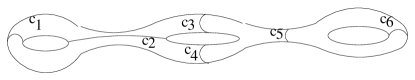
Figure 4: Maximal collection of simple loops

Then removing these circles we get

$$\Sigma-\{C_{1},...,C_{3g-3}\}=\cup_{i=1}^{2g-2}\tilde{v_{i}}$$ (4.8)

is a finite set of trinions (or ”pairs of pants”).

A trinion (or ”pair of pants”) plays the role of points in algebraic geometry under investigations of geometry of connections: just like we restrict functions to a point we can restrict connections to a trinion. Roughly speaking, a trinion is the minimal geometrical object admitting non trivial non-abelian gauge theory.

Riemann surface with a trinion decomposition (4.8) is called marked Riemann surface. Any marked surface defines the dual trivalent graph $\Gamma$

1. the set of vertices of which

   $$V(\Gamma)=\{v_{i}\}=\{\tilde{v_{i}}\}$$ (4.9)

   is the set of trinions;

2. and with the set of edges

   $$E(\Gamma)=\{e_{i}\}=\{C_{i}\};$$ (4.10)

3. and two vertices $v_{i}$ and $v_{j}$ are joined by the edge $e_{l}$ iff the corresponding circle

   $$C_{l}=\partial\tilde{v_{i}}\cap\partial\tilde{v_{j}}.$$ (4.11)

4.2 Real polarization

Every marked Riemanian surface $\Sigma_{\Gamma}$ defines a real polarization of the prequantized phase space

$$(CLRep(\pi_{1},\operatorname{SU}(2)),\omega,L,A_{CS}).$$ (4.12)

It is given in a very geometric way in the set-up of perturbation theory of 3-dimensional Chern–Simons theory. As we saw, a mark of Riemann surfaces is given by the choice of maximal collection of disjoint, noncontractable, pairwise nonisotopic smooth circles on $\Sigma$. Any such system contains $3g-3$ simple closed circles (4.7).

The isotopy class of a trinion decomposition $\{C_{i}\}$ gives the map

$$\pi_{\Gamma}\colon CLRep(\pi_{1},\operatorname{SU}(2))\to\mathbb{R}^{3g-3}$$ (4.13)

with fixed coordinates $(c_{1},\dots,c_{3g-3})$ such that

$$c_{i}(\pi_{\{C_{i}\}}(\rho))=\frac{1}{\pi}cos^{-1}(\frac{1}{2}tr\rho([C_{i}]))\in[0,1].$$ (4.14)

which are just Goldman functions (4.1).

Thus

1. this map is the moment map for the Hamiltonian $U(1)^{3g-3}$-action on $CLRep(\pi_{1},\operatorname{SU}(2))$, thus gives a real polarization of the system (4.12).

2. The coordinates $c_{i}$ are action coordinates for this Hamiltonian system ( [GS1]).

These functions $c_{i}$ are continuous on all $CLRep(\pi_{1},\operatorname{SU}(2))$ and smooth inside of the unit cube $[0,1]^{3g-3}$.

Thus we have

1. The image of $CLRep(\pi_{1},\operatorname{SU}(2))$ under $\pi_{\Gamma}$ is a convex polyhedron

   $$\Delta_{\Gamma}\subset[0,1]^{3g-3}.$$ (4.15)

2. The symplectic volume of $CLRep(\pi_{1},\operatorname{SU}(2))$ is equal to the Euclidean volume of $\Delta_{\Gamma}$:

   $$\int_{CLRep(\pi_{1},\operatorname{SU}(2))}\omega^{3g-3}=Vol\Delta_{\Gamma}.$$ (4.16)

3. The set of Bohr–Sommerfeld orbits of the real polarization $\pi_{\Gamma}$ of level $k$

   $$BS_{k}(\pi_{\Gamma},CLRep(\pi_{1},\operatorname{SU}(2)),\omega,L,A_{CS})$$ (4.17)

   is the set of $1/2k$- integer points in the polyhedron $\Delta_{\Gamma}$, and

   $$lim_{k\to\infty}k^{3-3g}\cdot N_{k-BS}=\int_{CLRep(\pi_{1},\operatorname{SU}(2))}\omega^{3g-3}=Vol\Delta_{\Gamma}$$ (4.18)

   just as predicted by general quantization rules.

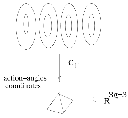
Figure 6: Moment map

To see the statements about Bohr-Sommerfeld fibers remark that every vector $w\in\mathbb{R}^{3g-3}$ can be interpreted as a differential $1$-form on $\mathbb{R}^{3g-3}$, and by the usual construction using the symplectic form $\Omega$, this defines a vector field $\xi_{w}$ tangent to the fibers of $\pi$. Integrating such vector fields, one defines the collection of transformations

$$\{t_{w}\}=\{e^{\xi_{w}}\}\subset Diff^{+}(CLRep(\pi_{1},\operatorname{SU}(2)).$$ (4.19)

These transformations preserve the curvature form of the connection $A_{CS}$. Thus (because $CLRep(\pi_{1},\operatorname{SU}(2))$ is simple connected), there exists a collection of gauge transformations $\alpha_{w}\in\mathcal{G}_{L}$ of $L$ such that

$$(t_{w})^{*}(A_{CS})=A_{CS}^{\alpha_{w}}$$ (4.20)

(see [AB] for the description of the gauge-orbit with fixed curvature form)

We can view such gauge transformations as $U(1)$-torsors, just as in the description of the formulas for classical theta functions for Abelian varieties (2.49). From this the subset $BS_{k}\subset\Delta_{\Gamma}$ of Bohr-Sommerfeld fibers of level $k$ is the subset of $1/2k$-integer points of $\Delta$.

To describe the polyhedron $\Delta_{\Gamma}$ we have to describe the space of flat $\operatorname{SU}(2)$-connections on a trinion $pp$ (pair of pants): let

$$\partial pp=C_{1}\cup C_{2}\cup C_{3}.$$ (4.21)

Then we have the map

$$\pi\colon CLRep(\pi_{1}(pp),\operatorname{SU}(2))\to\mathbb{R}^{3}$$ (4.22)

with fixed coordinates $(c_{1},c_{2},c_{3})$ just like in (3.139). It is easy to check (see [JW1]) the following fact

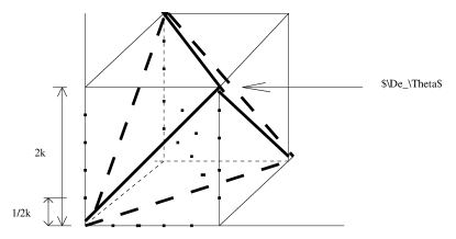
Figure 7: Moment tetrahedron

Proposition 17

1. the image

   $$\pi(CLRep(\pi_{1}(pp),\operatorname{SU}(2))=\Delta_{\Theta}$$ (4.23)

   is the tetrahedron given by the following inequalities

   $$0\leq c_{i}\leq 1,\quad|c_{1}-c_{2}|\leq c_{3}\leq min(c_{1}+c_{2},2-c_{1}-c_{2});$$ (4.24)

2. $\pi$ is 1-1 map, smooth inside of the tetrahedron and continious everywhere.

Using the dual 3-valent graph $\Gamma$ of the trinion decomposition (4.8) we can describe the polyhedron $\Delta_{\Gamma}$ (4.15):

Proposition 18

The polyhedron $\Delta_{\Gamma}$ is given by inequalities (4.24) for every triple $(c_{i},c_{j},c_{k})$ of the coordinates in $\mathbb{R}^{3g-3}$ corresponding to a boundary of any trinion in the decomposition (4.8).

4.3 Bohr-Sommerfeld fibers

In these terms we can describe Bohr-Sommerfeld fibers (using action coordinates $c_{i}$ ) as functions

$$w\colon E(\Gamma)\to\frac{1}{2k}\{0,1,2,\dots,k\}$$ (4.25)

on the collection of edges of the 3-valent graph $\Gamma$ to the collection of $\frac{1}{2k}$ - integers, such that, for any three edges $e_{1},e_{2},e_{3}$ meeting at a vertex $v$, the following 3 conditions hold:

1. $w(e_{1})+w(e_{2})+w(e_{3})\in\frac{1}{k}\cdot\mathbb{Z}$;

2. $w(e_{1})+w(e_{2})+w(e_{3})\leq 1$;

3. and

   $$|w(e_{1})-w(e_{2})|\leq w(e_{3})\leq min(w(e_{1})+w(e_{2}),2-w(e_{1}-e_{2})).$$ (4.26)

Such a function $w$ is called an admissible integer weight of level $k$ on the graph $\Gamma$.

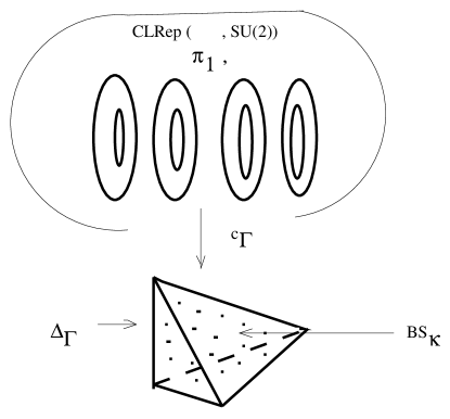
Figure 8: Bohr-Sommerfeld fibers

Let $W^{k}(\Gamma)$ be the set of such weights.

Remark

The geometrical meaning of the last inequality (4.26) is the following: it is the triangle inequality for triangles on 2-sphere. Thus if we do our graph flat that is fix a cyclic orientation around every vertex and write down around every vertex a triangle with sides orthogonal to edges and of lengths $w(e_{1}),w(e_{2}),w(e_{3}))$, identifying equal sides we get triangulated Riemann surface $\Sigma_{w}$ which is a finite combinatorial cover of $S^{2}$

$$\phi_{w}\colon\Sigma_{w}\to S^{2}.$$ (4.27)

For small genus, for example for the graph $\Theta$, this cover has degree one and gives just a triangulation of the basic sphere $S^{2}$. But from metric point of view this is a $1/2k$-integer triangulation.

Here is the list of simple but very important properties of weights:

Proposition 19

1. the number $|W^{k}(\Gamma)|$ of admissible weights of level $k$ is independent of the graph $\Gamma$ but depends on genus $g$ only;

2. $$|W^{k}(\Gamma)|=|W_{g}^{k}|=\frac{(k+2)^{g-1}}{2^{g-1}}\sum_{n=1}^{k+1}\frac{1}{(\sin(\frac{n\pi}{k+2}))^{2g-2}}$$ (4.28)

   is the Verlinde number (3.126).

To describe the geometry of Bohr-Sommerfeld fibers given by an admissible integer weight $w$ (4.25) we have to consider the levels of this function: for $\alpha\in\{0,\frac{1}{2k},\dots,1\}$ let

$$w^{-1}(\alpha)=\Gamma_{1}(\alpha)\cup\cdots\cup\Gamma_{n}(\alpha)\subset\Gamma$$ (4.29)

be the decomposition into connected components. Then every component $\Gamma_{i}(\alpha)$ is a 3-valent graph with $n_{i}$ univalent vertices $a_{1},\dots,a_{n_{i}}$ (see section 6).

Every gauge class of connections contains a connection $a_{0}$ adapted to a trinion decomposition (see [JW1], Definition 2.2). Fix the filtration

$$Z(\operatorname{SU}(2))=\mathbb{Z}_{2}\subset U(1)\subset\operatorname{SU}(2),$$ (4.30)

and view it as the triple $\{\mathbb{Z}_{2},U(1),\operatorname{SU}(2)\}$

For a connection $[a]\in\pi^{-1}(w)$, we have the function

$$e_{w}\colon E(\Gamma)\to\{\mathbb{Z}_{2},U(1),\operatorname{SU}(2)\}$$ (4.31)

sending every loop $C_{j}$ to the element of $G$ conjugate to the stabilizer of the monodromy of $[a]$ around this loop, and the function

$$v_{w}\colon V(\Gamma)\to\{\mathbb{Z}_{2},U(1),\operatorname{SU}(2)\}$$ (4.32)

sending trinion $P_{i}$ to the stabilizer of the flat connection $a_{{\textstyle{|}}P_{n}}$. Of course,

$$C_{j}\subset\partial P_{n}\implies v_{w}(P_{n})\subset e_{w}(C_{j});$$

$$C_{1}\cup C_{2}\cup C_{3}=\partial P_{n}\quad\text{and}\quad e_{w}(C_{1})=e_{w}(C_{2})=\operatorname{SU}(2)\implies$$ (4.33)

$$\qquad\qquad e_{w}(C_{3})=\operatorname{SU}(2)\implies v_{w}(P_{n})=\operatorname{SU}(2),$$

and so on.

Obviously

$$e_{w}(C_{j})=\text{$U(1)$ or $\operatorname{SU}(2)$.}$$ (4.34)

Proposition 20

The functions $e_{w}$ and $v_{w}$ depend on $w$ and not on the choice of $[a]\in\pi^{-1}(w)$.

More precisely, they depend on the combinatorics of the decomposition (4.29).

Thus $w$ defines the direct products

$$\prod_{C\in E(\Gamma)}e_{w}(C)\quad\text{and}\quad\prod_{P\in V(\Gamma)}v_{w}(P),$$

and $\prod_{P\in V(\Gamma)}v_{w}(P)$ acts on $\prod_{C\in E(\Gamma)}e_{w}(C)$ as follows: for

$$g=(g_{1},\dots,g_{2g-2})\in\prod_{P\in V(\Gamma)}v_{w}(P)\quad\text{with $g_{i}\in v_{w}(P_{i})$, and}$$

$$(t_{1},\dots,t_{3g-3})\in\prod_{C\in E(\Gamma)}e_{w}(C)\quad\text{with $t_{n}\in e_{w}(C_{n})$,}$$

if $C_{n}\subset\partial P_{i}\cap\partial P_{j}$ then

$$g(t_{n})=g_{i}\circ t_{n}\circ g_{j}^{-1}.$$ (4.35)

Remark

This action described in detail in subsection 6.3 under the consideration of the gauge theory on graphs.

Proposition 21 ([JW1], Theorem 2.5)

The fibre $\pi^{-1}(w)$ is given by

$$\pi^{-1}(w)=\prod_{C\in E(\Gamma)}e_{w}(C)\Bigm{/}\prod_{P\in V(\Gamma)}v_{w}(P).$$ (4.36)

Corollary 1

The fibre $\pi^{-1}(w)$ is isomorphic to

$$\pi^{-1}(w)=T^{t}\times[(S^{3})^{p}\times(S^{2})^{s}]/G_{w},$$ (4.37)

where $t,p$ and $s$ are nonnegative integers and $G_{w}$ is the finite Abelian group defined by $w$, or more precisely by the combinatoric data (4.1); moreover,

$$H_{1}(\pi^{-1}(w))=\mathbb{Z}^{t}\oplus\mathbb{Z}_{2}^{p}.$$ (4.38)

Translations along the torus $T^{t}$ in (4.37) are induced by Hamiltonians lifted from the target space $\mathbb{R}^{3g-3}$ of $\pi$.

Jeffrey and Weitsman [JW1] use the normalization of the action coordinates via branched covers to construct a covariant constant section $s_{w}$ of the restrictions of $(L^{k},A_{CS})$ to $\pi^{-1}(w)$.

Following the real polarization quantization rules from section 1 (formula (1.21)) the wave function space is given by the direct sum

$$\mathcal{H}^{k}_{\Gamma}=\oplus_{b\in BS_{k}}\mathbb{C}\cdot s_{b}$$ (4.39)

where $s_{b}$ is a covariant constant section of the restriction of our line bundle and connection to $\pi^{-1}(b)$.

Geometrically this combinatorial description of Bohr-Sommerfeld fibers can be done as follows: consider the space $\mathbb{R}^{3g-3}$ with action coordinates $c_{i}$ (4.14). This space contains the integer sublattice $\mathbb{Z}^{3g-3}\subset\mathbb{R}^{3g-3}$, and we can consider the action torus:

$$T^{A}=\mathbb{R}^{3g-3}/\mathbb{Z}^{3g-3}.$$ (4.40)

In particular, we get a map

$$\pi_{A}\colon CLRep(\pi_{1},\operatorname{SU}(2))\to T^{A}$$ (4.41)

which glues at most points of the boundary of $\Delta_{\Gamma}$.

Now every integer weight $w$ (4.25) satisfying (1) and (2), but a priori without the Clebsch–Gordan conditions (3) (4.26), defines a point of order $2k$ on the action torus

$$w\in T^{A}_{2k}.$$

In particular, the collection $W^{k}(\Gamma)$ of admissible integer weights (subject to (3) (4.26)) can be considered as a subset of points of order $2k$ on the action torus:

$$W^{k}(\Gamma)\subset T^{A}_{2k}.$$ (4.42)

Thus for different $\Gamma$ of genus $g$ we have a priori different subsets $\{W^{k}(\Gamma)\}$ of the set of points of order $2k$ on the action torus $T^{A}$ (4.40).

The linear decomposition of the wave function space (4.39) defines the space uniquely up to the coordinatewise $|W^{k}(\Gamma)|$-torus action because every covariant constant section is defined up to $U(1)$-action. But using admissible integer weights we can define this space as a space with a fixed basis

$$\mathcal{H}^{k}_{\Gamma}=\oplus_{w\in W^{k}_{\Gamma}}\mathbb{C}\cdot w$$ (4.43)

and the integer sublattice

$$\mathbb{Z}^{|W^{k}_{\Gamma}|}\subset\mathcal{H}^{k}_{\Gamma}.$$ (4.44)

All of these spaces are embedded in one large space

$$\mathcal{H}^{k}_{\Gamma}\subset\mathcal{H}^{k}=\oplus_{w\in T^{A}_{2k}}\mathbb{C}\cdot w$$ (4.45)

(see (4.42)) with the integer lattice

$$\mathbb{Z}^{|T^{A}_{2k}|}\subset\mathcal{H}^{k}.$$ (4.46)

4.4 Delzant model

Returning to the moment map (3.148) we come into the set-up of the toric symplectic geometry: let $(M,\omega)$ be a compact symplectic smooth manifold of dimesion $2n$ with a smooth Hamiltonian action of $n$-dimensional torus $T^{n}$. Then action-angle coordinates define the moment map

$$\pi\colon M\to\Delta\subset\mathbb{R}^{n}$$ (4.47)

whose image is a convex polyhedron $\Delta$ in Euclidean $n$-space. This polyhedron satisfies so called Delzant conditions and contains complete information on the symplectic geometry of $(M,\omega)$. That is, $\Delta$ determines the manifold, the symplectic form and the $T^{n}$-action (see [D]). Moreover, if a polyhedron $\Delta\subset\mathbb{R}^{n}$ satisfies the Delzant conditions then we can construct a smooth symplectic manifold with Hamiltomian $T^{n}$-action such that the image of the moment map is precisely $\Delta$.

Moreover, if a phase space $(M,\omega)$ is prequantized and $M$ has a Hodge structure whose Kahler form is $\omega$, then this Hodge structure can also be reconstructed from $\Delta$ (see [G1]).

We saw that our space $CLRep(\pi_{1}(\Sigma),\operatorname{SU}(2))$ admits the Hamiltonian $T^{3g-3}$-torus action, but

1. our phase space $CLRep(\pi_{1}(\Sigma),\operatorname{SU}(2))$ is singular if $g>2$;

2. the action isn’t smooth over the boundary of $\Delta$.

Nevertheless the polyhedron satisfies Delzant conditions hence determines the smooth compact Hodge manifold $DM_{\Gamma}$ with the smooth $T^{3g-3}$-action which is called Delzant model of moduli spaces (see [T8]). For a complex Riemann surface $\Sigma_{I}$ the moduli space $M^{ss}(\Sigma_{I})$ is an algebraic variety. Every such variety admits a birational morphism

$$f\colon M^{ss}(\Sigma_{I})\to DM_{\Gamma}.$$ (4.48)

The list of properties is the following

1. The Delzant model $DM_{\Gamma}$ is canonically polarized by the line bundle $H$ corresponding to the theta polarization of every $M^{ss}$.

2. The Delzant model is rigid as a complex manifold and hence the Kahler quantization of $(DM_{\Gamma},H)$ is succesful. The wave function spaces are given as spaces of holomorphic sections

   $$H^{0}(DM_{\Gamma}),H^{k})$$ (4.49)

   and dimensions of these spaces can be computed by the Duistermaat-Heckman formula.

3. Bohr-Sommerfeld fibers for $CLRep(\pi_{1}(\Sigma),\operatorname{SU}(2))$ and $DM_{\Gamma}$ as sets of points of $\Delta_{\Gamma}$ coincide.

4. The rank of wave spaces (4.49) is equal to the number of Bohr-Sommerfeld fibers thus the quantization of the dynamical system $(DM_{\Gamma},\omega)$ is numericaly perfect (see [T8]).

5 Two versions of CQFT

Result of any quantization procedure is creation of a quantum mechanics which is QFT in dimension d = 1 when there is only one variable - a time. But our main geometrical object - Riemann surfaces - are also the basic object of conformal field theories in dimension 2 (or, more precisely, (1,1)).

Some years ago the constraint of conformal invariance was proposed as the fundamental principle of quantum field theory. All two-dimensional conformal field theories are duing to the theory of critical phenomena and to the string theory. So, the new powerful mathematical tool appeared since large data on the geometry of Riemann surfaces is encoded in this rich mathematical structure. Moreover, the results of a succesful Kahler quantization procedure = the wave function spaces $H^{0}(M^{ss}(\Sigma),\mathcal{O}(k\Theta))$ appeared first as spaces of conformal blocks of CQFT.

On the other hand, the spaces $\mathcal{H}_{\pi}^{k}=\oplus_{b\in BS_{k}\subset B}\mathbb{C}\cdot s_{b}$ as results of the Bohr-Sommerfeld quantization procedure appeared as fibers of projective flat vector bundles over the moduli space $\mathcal{M}_{g}$ of curves of genus $g$ in the combinatorial version of CQFT in [FS] and [MS]. Moreover, a 2-dimensional conformal field theory was formulated as algebraic geometry of the moduli spaces of Riemann surfaces.

A very important case of that a pinched Riemann sphere was investigated by Belavin-Knijnik-Zamolodchikov in [KZ] which produce the general ideology as well as thechnical fondations.

We can start with the simple ”classical” version of CFT.

5.1 WZW-version

Recall that the space of classical theta functions has very important property to be a space of unique irreducible representation of some group or algebra (namely the Heisenberg group). The space of holomorphic sections $H^{0}(M^{ss}(\Sigma),\mathcal{O}(k\Theta))$ is also the space of the irreducible representation of the gauge algebra of WZW RCFT. Such spaces have played a noted role in conformal field theory.

It turn out that in rational conformal field theories, one encounters the ”conformal blocks” of Belavin, Polyakov and Zamolodchikov coincidencing with our spaces $H^{0}(M^{ss}(\Sigma),\mathcal{O}(k\Theta))$ .

First of all recall Wess-Zumino-Witten CQFT (WZW for short) set up: let $t$ be a local parameter in a point $p\in\Sigma$. Then the loop algebra

$$sl_{2}^{t}=sl(2,\mathbb{C})\otimes\mathbb{C}[t,t^{-1}]$$ (5.1)

is the horisontal algebra of WZW.

The central extention by the cocycle $k\cdot c$

$$\overline{sl_{2}^{t}}=sl(2,\mathbb{C})\otimes\mathbb{C}[t,t^{-1}]\oplus\mathbb{C}\cdot e$$ (5.2)

is the k-gauge algebra of WZNW and the bracket of two elements of the loop algebra is given by the formula

$$[X\otimes f,Y\otimes g]=[X,Y]\otimes fg+k\cdot tr(XY)Res_{0}(gdf)$$ (5.3)

The theory of Kac-Moody algebras tells us that this algebra admits unique irreducible representation $\mathcal{H}^{k}$ such that there exists a non-zero vector annihilated by $sl(2,\mathbb{C})\otimes\mathbb{C}[t]$. Remark that the central element of $\overline{sl_{2}^{t}}$ acts by multiplication by $k$ (which is the level number).

On the other hand, the field $\mathbb{C}(\Sigma)$ of meromorphic functions on $\Sigma$ has the natural embedding:

$$i\colon sl(2,\mathbb{C})\otimes\mathbb{C}(\Sigma)\to\overline{sl_{2}^{t}}.$$ (5.4)

This field $\mathbb{C}(\Sigma)$ contains the subring $\mathbb{C}(\Sigma)_{p}$ of regular functions in $\Sigma-p$. The structure of algebra on

$$sl(2,\mathbb{C})\otimes\mathbb{C}(\Sigma)_{p}$$ (5.5)

is given by the formula

$$[X\otimes f,Y\otimes g]=[X,Y]\otimes fg$$ (5.6)

The restriction of the embedding (4.4) to this subring realizes it as the subalgebra of $\overline{sl_{2}^{t}}$.

Thus the algebra $sl(2,\mathbb{C})\otimes\mathbb{C}(\Sigma)_{p}$ acts on the representation $\mathcal{H}^{k}$ described before.

Definition 8

The space of conformal blocks $V_{k}$ of level $k$ is the subspace of the dual $(\mathcal{H}^{k})^{*}$ annihilated by the Lie algebra $sl(2,\mathbb{C})\otimes\mathbb{C}(\Sigma)_{p}$.

Why such space is related to vector bundles on $\Sigma$? First of all, we note, that every vector bundle $E$ on $\Sigma-p$ is trivial and of course it is trivial on a small disc $D_{p}$ containing $p$. Fixing these trivializations we send a vector bundle $E$ to the Laurent series

$$\gamma_{E}\in SL(2,\mathbb{C})\otimes\mathbb{C}[t,t^{-1}].$$ (5.7)

To get rid of the trivializations, we have to mod out by the automorphisms groups of trivial bundles on $D_{p}$ and $\Sigma-p$. So the set of vector bundles is

$$\{E\}=SL(2,\mathbb{C})\otimes\mathbb{C}(\Sigma)_{p}\backslash\operatorname{\mathcal{\mathfrak{sl}}}(2,\mathbb{C})\otimes\mathbb{C}[t,t^{-1}]/SL(2,\mathbb{C})\otimes\mathbb{C}[t].$$ (5.8)

Remark that we don’t discuss the stability condition and our double coset space is so called algebraic stack, not a moduli space.

In any case our, stack $\{E\}$ is the quotient of the universal homogeneous space

$$Q=SL(2,\mathbb{C})\otimes\mathbb{C}[t,t^{-1}]/SL(2,\mathbb{C})\otimes\mathbb{C}[t]$$ (5.9)

and the line bundle $\mathcal{O}(\Theta)$ can be lifted to the universal line bundle $L_{\chi}$ on this homogeneous space. The theorem of Kumar and Mathueu provides the isomorphism

$$H^{0}(Q,L_{\chi}^{k})=\mathcal{H}^{k}$$ (5.10)

and $H^{0}(M^{ss},Oh(k\Theta))$ coincides with the subspace of $(\mathcal{H}^{k})^{*}$ invariant under Lie algebra $sl(2,\mathbb{C})\otimes\mathbb{C}(\Sigma)_{p}$ action.

To see that this space is finite dimensional over $\mathbb{C}$, we need only the standard experience with matrix divisors (for example, like in the survey [T2]). But to compute the dimension we have to use more sophisticated versions of all objects.

First of all, on our Riemann surface $\Sigma$ we choose a finite set of different points

$$p_{1},p_{2},.....,p_{n}\subset\Sigma$$ (5.11)

different from our fixed point $p\in\Sigma$ and labeled by the set of irreducible representations of $sl(2,\mathbb{C})$, that is, by positive integers $n_{1},n_{2},....,n_{n}$ (twice spin-numbers).

Now our algebra $sl(2,\mathbb{C})\otimes\mathbb{C}(\Sigma)_{p}$ acts on the space $V_{n_{i}}$ of the irreducible representation $n_{i}$ by the formula

$$(X\otimes f)v=f(p_{i})Xv$$ (5.12)

where $p_{i}$ is the point corresponding to the representation $n_{i}$ and $v\in V_{n_{i}}$.

New vector space is given now by the formula

$$V_{k}(\{(p_{i},n_{i})\})_{\Sigma}=Hom_{sl(2,\mathbb{C})\otimes\mathbb{C}(\Sigma)_{p}}(\mathcal{H}^{k},\otimes_{i=1}^{n}V_{n_{i}}).$$ (5.13)

These spaces have a number of good properties. For example, they don’t depend on moduli of curves, the choice of points and so on. But the most important property is the behavior with respect to a simplest degeneration of curve $\Sigma$ to curve $\Sigma_{0}$ with one double point. Geometrically this means that we have a smooth curve $\Sigma_{0}$ of genus $g-1$ with a fixed pair of points $(q_{+},q_{-})$. Then

$$V_{k}(\{(p_{i},n_{i})\})_{\Sigma}=\oplus_{n\in\mathbb{Z}^{+}}V_{k}(\{(p_{i},n_{i}),(q_{+},n),(q_{-},n)\})_{\Sigma_{0}}.$$ (5.14)

These properties provide the induction by genus (just like formula (3.107) ).

Now we are interested only in ranks of previous spaces. We may forget about curves, points and others geometrical features (how we did after (3.109) in subsection 3.7) and consider the monoid $M$ of formal sums

$$N=n_{1}+n_{2}+...+n_{n}\in M$$ (5.15)

providing the present labeling of points. Every rank of space $V_{k}(\{(p_{i},n_{i})\})_{\Sigma}$ can be done as a symbol

$$rk_{g}(N),\quad\text{where}\quad N=n_{1}+n_{2}+...+n_{n}\in M.$$ (5.16)

The list of properties of these numbers is the following:

1. $rk_{0}(0)=1;$

2. $rk_{g}(N)=\sum_{n\in\mathbb{Z}^{+}}rk_{g-1}(N+n+n)$;

3. let $g=g^{\prime}+g^{\prime\prime}$, then

   $$rk_{g}(N^{\prime}+N^{\prime\prime})=\sum_{n\in\mathbb{Z}^{+}}rk_{g^{\prime}}(N^{\prime}+n)\cdot rk_{g^{\prime\prime}}(N^{\prime\prime}+n).$$ (5.17)

Using these equalities, we can decent genus $g$ to 0 and get so called fusion rules:

1. $rk_{0}(0)=1$;

2. $rk_{0}(N^{\prime}+N^{\prime\prime})=\sum_{n\in\mathbb{Z}^{+}}rk_{0}(N^{\prime}+n)rk_{0}(N^{\prime\prime}+n)$.

These fusion rules give the structure of commutative ring on our monoid $M$:

$$N\cdot N^{\prime}=\sum_{n\in\mathbb{Z}^{+}}rk_{0}(N+N^{\prime}+n)\cdot n.$$ (5.18)

This commutative ring is called the fusion ring.

Remark

We don’t prove here the factorisation rules (5.17) in the algebraic geometrical set-up, that is, in the set-up of vector bundles. We will get them as bypass results at the end of our long story. But remark that there are exist approaches to prove these rules in purely geometrical way.

We saw that our fusion ring is very close to be the ring of irreducible representations $R(sl(2,\mathbb{C}))$ where the multiplication is the tensor product of representations. But there is a small difference coming from level $k$ condition.

According to the Clebsh-Gordan rules, a tensor product of irreducible representation has the decomposition:

$$n_{1}\otimes n_{2}=(n_{1}+n_{2})\oplus(n_{1}+n_{2}-2)\oplus....\oplus(n_{1}-n_{2})$$ (5.19)

(here $n_{1}\geq n_{2}$). But the level condition is $n\leq k$ and the multiplication is given by the formulas:

1. $n_{1}+n_{2}\leq k\implies n_{1}\circ n_{2}=n_{1}\otimes n_{2}$;

2. $n_{1}+n_{2}\geq k\implies n_{1}\circ n_{2}=(2k-n_{1}-n_{2})\oplus...\oplus(n_{1}-n_{2})$.

From this it is easy to see that the fusion ring $M_{k}$ of level $k$ is the quotient of $R(sl(2,\mathbb{C}))$ by the ideal generated by $(k+1)$.

The fusion ring $M_{k}$ has the element

$$c=\sum_{n=0}^{k}n\circ n.$$ (5.20)

Let $SpecM_{k}$ be the set of characters (homomorphisms to $\mathbb{C}$) of $M_{k}$. Then after elementary computations we get the equality

$$rk_{g}(\emptyset)=\sum_{\chi\in SpecM_{k}}\chi(c)^{g-1}$$ (5.21)

and

$$\chi(c)=\sum_{n=0}^{k}|\chi(n)|^{2}.$$ (5.22)

Recall that every character of the representations ring $R(sl(2,\mathbb{C}))$ is given by $z\in\mathbb{C}$ and

$$\chi_{z}(n)=\frac{sin((n+1)z)}{sinz}.$$ (5.23)

This character is from $SpecM_{k}$, that is, it vanishes on $(k+1)$ iff

$$z=\frac{n\pi}{k+2},\quad(1\leq n\leq k+1).$$ (5.24)

Now elementary computations and formula (8.35) give

$$rk_{g}(\emptyset)=rkV_{k}=\frac{(k+2)^{g-1}}{2^{g-1}}\sum_{n=1}^{k+1}\frac{1}{(\sin(\frac{n\pi}{k+2}))^{2g-2}}$$ (5.25)

which is the Verlinde number again.

In the conformal blocks set up very important observation is the absence of Hermitian structure on all vector spaces of this theory. Indeed we are working always with ”sl” objects, not with ”su”. This feature is distiguishing from the quantization set up where Hermitian structure appears manifestly.

5.2 WZW-connection

On the moduli space $\mathcal{M}_{g,1}$ of curves of genus $g$ with a fixed (pinched) point we have vector bundles (1.29) interpreted as vector bundles of conformal blocks. This identification induces another interpretation of the Hitchin’s projective flat connection coming from CQFT (see [TK] or beautiful survey [S]).

The construction and investigation of the connection in these terms are almost parallel to the constructions described in subsection 3.8. The difference is following: instead of the moduli space of Higgs bundles (which is nothing else as the space of $SL(2,\mathbb{C})$-representations of the fundamental group of Riemann surface) we consider the infinite dimensional space $Q$ (5.9) and lift all of our problems to it. Actually before that we have to develop a technique of working with infinite dimensional objects of such type rigorously. This was done in [BL]. Saveing the time-space here we describe this approach only briefly.

Recall that the ind-homogeneous (”ind” is a term from [BL]) space $Q$ (5.9) describes $\operatorname{SU}(2)$-vector bundles trivialized on $\Sigma-p$ where $(\Sigma,p)\in\mathcal{M}_{g,1}$. Of course we consider the dense open subset

$$Q_{0}\subset Q$$ (5.26)

corresponding to semi-stable bundles. For this space the following fact was proved in [DS]: the natural map

$$f\colon Q_{0}\to M^{ss}(\Sigma)$$ (5.27)

is a locally trivial torsor in the etale topology. (The proof of this fact is contained also in unpublished preprint of Beilinson and Kazhdan.)

In this set up Yves Laszlo constructed a family of second order differential operators $\theta(\dot{I})$ over the family of deformations of complex structures. This construction commutes with the construction given by the composite morphisms $\phi_{s}$ (1.86) with the cohomology sequence of the exact triple (1.81) which gives

$$H^{1}(\Sigma,T\Sigma)\to H^{0}(S^{2}(TM^{ss}(\Sigma)))\to H_{h}^{1}(d_{s}).$$ (5.28)

This lifting is, in a sense, a lifting of the Sugawara tensor $T(\dot{I})$ (modulo the ind-scheme technique). Namely for every function $f$ on $\mathcal{M}_{g,1}$ and a local section $\tilde{e}$ of the family of dual to (5.10) spaces, the WZW-connection is given by the formula

$$\nabla(f\otimes\tilde{s})=\dot{I}(f)\cdot\tilde{s}+\frac{1}{2k-4}\cdot T(\dot{I})\tilde{s}\otimes f\quad mod(\tilde{s}\otimes f).$$ (5.29)

From this point the equality of both connections is obvious because the only non trivial term in the previous formula is the Sugawara term just as in the formula (3.152). Thus the Hitchin’s connection is the WZW-connection indeed.

5.3 Monodromy representations

All of our projective and vector connections are on vector bundles over the Teichmuller space $\tau_{g}$. The modular group

$$Mod_{g}=Diff^{+}\Sigma/Diff_{0}\Sigma$$ (5.30)

acts on the Teihmuller space $\tau_{g}$ such that

$$\mathcal{M}_{g}=\tau_{g}/Mod_{g}.$$ (5.31)

Thus all of them define projective or vector representation of the modular group $Mod_{g}$

$$\rho\colon Mod_{g}\to PGL(N_{k},\mathbb{C})$$ (5.32)

where $N_{k}$ is rank of the vector bundle $V_{k}$.

For example, for the classical theory of theta functions we have two vector representations

$$Mon_{w}^{k}\colon Mod_{g}\to PGL(k^{g},\mathbb{C})$$ (5.33)

given by the Welters projective flat connection, that is, by applying the full procedure of extended Kodaira-Spencer theory (see [W]). On the other hand, the symplectic theory yields another combinatorial connection (see [K1] and another monodromy representation

$$Mon_{BS}^{k}\colon Mod_{g}\to PGL(k^{g},\mathbb{C}).$$ (5.34)

Fortunately, the perfect quantization identifies both of these connections and representations to give unique abelian representation

$$Mon_{w}^{k}=Mon_{BS}^{k}=Mon^{k}_{a}.$$ (5.35)

Moreover, the monodromy group of this representation is finite

$$Mon_{k}^{a}=Sp(2g,\mathbb{Z}_{2k}).$$ (5.36)

For non-abelian case we have the representation

$$Mon_{H}^{k}\colon Mod_{g}\to PGL(rk_{g}(\emptyset),\mathbb{C})$$ (5.37)

given by the Hitchin connection.

On the other hand, using identifications from [TUY] and [TK] Kohno constructed this representation in the pure combinatorial way

$$Mon_{c}^{k}\colon Mod_{g}\to PGL(rk_{g}(\emptyset),\mathbb{C}).$$ (5.38)

(The subscript $"c"$ here stands for ”combinatorial”.) The lines decompositions (4.39) of fibers is parallel to the decomposition of the highest weight representation of the affine Lie algebra of $\operatorname{\mathcal{\mathfrak{sl}}}(2,\mathbb{C})$ by eigenspaces of the operator $L_{0}$ from Sugawara construction of the representation of the Virasoro Lie algebra (see [K2]). Manifestly this representation is projective Hermitian. It was investigated by Macsbaum and Funar. The main result is the following: the monodromy group of this representation is infinite if $k\neq 2,3,4,6$ and $k\neq 10$ for $g=2$.

Moreover, in paper [An] J. Andersen proved asymptotic faithfulness of the collection of representations that is the intersection of kernels

$$\bigcap_{k=1}^{\infty}kerMon^{k}_{H}=1\text{ or }\mathbb{Z}_{2}\text{ for }g=2.$$

(Of course this result is proved for any rank of vector bundles.) More precisely he proved that that Berezin-Toeplitz endomorphisms associated to smooth functions on $M^{ss}$ are asymmptotically flat.

The appearance of the Sugawara construction in the procedure of definition of this connection suggested the equivalence of these representations. It was proved using the Borthwick-Paul-Uribe method in [T3]. This method is quite different from CQFT and it will be productive to use generalized Sugawara construction [Sc] to get this coincidence directly as the generalization of Kniznik-Zamolodchikov construction.

6 3-valent graphs

6.1 Spin networks

Friedan and Shenker [FS], Moor and Seiberg [MS] proposed a new approach to CFT - the axiomatic description of a rational conformal field theory. We will call it the MS-axiomatic. The main ingredient of this theory is 3-valent graphs which appeared in constructions of section 4 already. We saw that every 3-valent graph is equivalent to a trinion-decomposed Riemann surface (see (4.9)-(4.11)).

In a similar way, we can extend these constructions to an orientable surface $\Sigma$ of genus $g$ with $n$ holes. Geometrically such surface with a trinion decomposition is equivalent to its dual 3-1-valent graph $\Gamma$ or a history (3-valent graph of genus $g$ with $n$ parabolic edges which we describe in the special subsection). In this case admissible integer weights are defined in the same way as in (4.25) and (4.26) but the set of weights

$$W^{k}(\Gamma,v_{1},\dots,v_{n})$$ (6.1)

is the set of functions $w$ (4.25)-(4.26) satisfying the conditions

$$w(a_{i})=v_{i}$$ (6.2)

for every parabolic edge $a_{i},\quad 1\leq i\leq n$, that is, the values of these functions on parabolic edges are fixed constants. So in the same vein we have spaces

$$\mathcal{H}^{k}_{\Gamma,v_{1},\dots,v_{n}}=\oplus_{w\in W^{k}(\Gamma,v_{1},\dots,v_{n})}\mathbb{C}\cdot w$$ (6.3)

The Clebsch–Gordan conditions (1), (2) and (3) from (4.26) provide a very surprising point of all these constructions: namely, let us multiply all our integer weights $w\in W^{k}(\Gamma)$ by level $k$. We get the maps

$$k\cdot w=j\colon E(\Gamma)\to 1/2\mathbb{Z}_{\geq 0}.$$ (6.4)

But we can consider the target set as the set of irreducible representations of $\operatorname{SU}(2)$:

$$\widehat{\operatorname{SU}(2)}=1/2\mathbb{Z}_{\geq 0}.$$ (6.5)

So every integer weight can be considered as a coloring of edges by irreducible representations of $\operatorname{SU}(2)$. The conditions (1), (2) and (3) (4.26) give that for every triple $e_{1},e_{2},e_{3}$ via one vertex $v$ the tensor product of representations

$$0\in j(e_{1})\otimes j(e_{2})\otimes j(e_{3})$$ (6.6)

that is this tensor product contains the trivial representation. Or the tensor product $j(e_{1})\otimes j(e_{2})$ admits an intertwiner

$$i_{v}\colon j(e_{1})\otimes j(e_{2})\to j(e_{3})$$ (6.7)

as $\operatorname{SU}(2)$-equivariant homomorphism.

Such coloring of graph edges is called $\operatorname{SU}(2)$-spin network by Penrose [P]( see also [T1]). Thus the set $W^{k}(\Gamma)$ is the set of spin networks of level $k$ over a graph $\Gamma$. We will see in the following section that for every integer weight $w\in W^{k}(\Gamma)$ the function

$$2k\cdot w=t\colon E(\Gamma)\to\mathbb{Z}_{\geq 0}.$$ (6.8)

is the type of a loop on our graph $\Gamma$. It means, that a colouring can be defined purely in terms of the geometry of graph as a topological space.

The main fact here is the identification of the set $SNW^{k}(\Gamma)$ of $\operatorname{SU}(2)$-spin networks of level $k$

$$SNW^{k}_{\Gamma}=W^{k}(\Gamma)$$

and the set of integer weights $W^{k}(\Gamma)$.

Our first task is to compare spaces $\mathcal{H}^{k}_{\Gamma}$ for different graphs of genus $g$. As a result of this comparing we will construct, following Kohno [K1], the holomorphic vector bundle with a holomorphic projective flat connection over the moduli space $\mathcal{M}_{g}$ of Riemann surfaces of genus $g$. This construction is purely topological. So first of all we have to construct combinatorial models of the Teichmuller space and the trivalent graphs complex. These ideas and constructions came from low dimensional topology and classical and quantum Conformal Field Theories.

Figure 9: Pumping up trick

6.2 3-dimensional topology

Recall again that any 3-valent graph is equivalent to a trinion decomposition of a Riemann surface. It is easy to see that such surface is a boundary of uniquely determined handlebody. We explain this fact more carefully.

Returning to a maximal set of disjoint inequivalent curves $\{C_{1},...,C_{3g-3}\}$ (4.7) and removing these curves we get a finite set of trinions $\Sigma-\{C_{1},...,C_{3g-3}\}=\cup_{i=1}^{2g-2}\tilde{v_{i}}$ (4.8) (see Fig.2).

Every oriented trinion defines the handlebody inside it and gluing (sewing) these handlebodies together we get the handlebody $H_{\Gamma}$ such that

$$\partial H_{\Gamma}=\Sigma_{\Gamma}$$ (6.9)

Any diffeomorphism $h\in Mod_{g}$ (where $Mod_{g}$ is the modular group (5.30)) gives us a compact 3-manifold

$$X_{\Gamma}=H_{\Gamma}\cup_{h}H_{\Gamma}$$ (6.10)

where we are gluing two handlebodies with the boundaries by the diffeomorphism

$$h\colon\partial H_{\Gamma}=\Sigma_{\Gamma}\to\Sigma_{\Gamma}=\partial H_{\Gamma}.$$ (6.11)

For the 3-manifold such presentation is called a Heegaard splitting. The subgroup

$$M_{\Gamma}\subset M_{g}$$ (6.12)

of diffeomorphisms which can be extended to diffeomorphisms of the handlebody $H_{\Gamma}$, acts on $Mod_{g}$ on the left and right and we have the set of 3-manifolds

$$\{X_{\Gamma}\}=M_{\Gamma}\backslash Mod_{g}/M_{\Gamma}$$ (6.13)

as the set of double cosets.

In Heegard splitting (6.10) let us add a new handle to the surface and extend the diffeomorphism $g$ by the identity on this new handle. This procedure doesn’t change our 3-manifold and is called stabilization. Singer proved in [Si] the following statement

Proposition 22

The equivalence relation between elements $h\in Mod_{g}$ when $g\to\infty$ creating homeoomorphic 3-manifolds, is generated by isotopies, left and right actions of $M_{\Gamma}$ and a stabilization.

To construct an invariant of 3-manifolds we have to send a marked Riemann surface $\Sigma_{\Gamma}$ to the wave function vector space $\mathcal{H}^{k}_{\Gamma}$ (4.43) with fixed vector $w_{H_{\Gamma}}$ given by the function (4.25) such that

$$w_{H_{\Gamma}}(e)=0\quad\text{for every}\quad e\in E(\Gamma).$$ (6.14)

Here

$$w_{H_{\Gamma}}\in\mathcal{H}^{k}_{\Gamma}$$ (6.15)

is called the vacuum vector for the handlebody $H_{\Gamma}$.

The space $\mathcal{H}^{k}_{\Gamma}$ admits the standard Hermitian structure which identifies this space with the dual.

Now if we have a linear representation

$$\rho\colon Mod_{g}\to GL(\mathcal{H}^{k}_{\Gamma})$$ (6.16)

then

$$I(X_{\Gamma,g})=\frac{<w_{H_{\Gamma}},\rho(g)(w_{H_{\Gamma}})>}{\|w_{H_{\Gamma}}\|^{2}}$$ (6.17)

has to be an invariant of $X_{\Gamma}$ as 3-manifold since it easy to see that

1. the vector $w_{H_{\Gamma}}$ is invariant with respect to $M_{\Gamma}$-action and

2. under normalization (6.17) this vector is invariant under stabilization.

But the situation is a slightly more complicated then just described. Namely, Kohno constructed nonlinear representation $\rho$ but made it slightly projective, that is, determined up to the usual phase amplitude

$$e^{\frac{\pi i\cdot k}{4(k+2)}}.$$ (6.18)

Thus the invariant (6.17) is determined up to the same phase amplitude.

To construct such slightly projective representation (6.16) one has to treat combinatorial constructions in the next special section.

6.3 Geometry of graphs

A graph is one dimensional complex containing edges - cells of one dimensional skeleton and vertices -cells of zero dimensional skeleton.

The combinatorial invariant of a pinched Riemann surfaces with a trinion decomposition is a (3-1)-valent graphs or a history. Such graphs have 3-valent and 1-valent vertices. The last vertices are half intervals with one vertex. Vertices of such edges are called parabolic.

Graphs and histories are Feynman diagrams - objects of the standard formalism in fields (for 3-valent graph case, $\phi^{3}$ - theories).

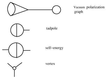
Figure 10: Standard Feynman diagrams

In classical and quantum field theory a 3-valent graph without parabolic vertices is called a vacuum-polarization graph. So we will consider such graph as a geometrical object. Note that an closed 1-valent graph is a disjoint finite union of compact intervals and a closed 2-valent graph is a disjoint finite union of compact circles.

Every graph $\Gamma$ has the following ingredients:

1. $E(\Gamma)$ is the set of edges;

2. $V(\Gamma)$ is the set of vertices,

3. $S(v)$ is the star of a vertex $v$ that is the set of local edges incident to $v$,

4. $F(\Gamma)=\{v\in e\}$ is the set of flags (edge + vertex). It is the same as the set of oriented edges $\vec{E}(\Gamma)$,

5. $L(\Gamma)$ is the set of circles, that is, of edges with only one vertex.

We will consider homogeneous graphs that is the graphs of the same valence $d$ at every vertex.

For example for 3-valent graphs two projections $p_{e}\colon F(\Gamma)\to E(\Gamma)$ and $v\colon F(\Gamma)\to V(\Gamma)$ are finite covers of degrees 2 and 3 with the same ramification locus $W_{e}=W_{v}\subset F(\Gamma)$, containing pairs $v\in e$, where $e$ is a loop:

$$R_{e}=L(\Gamma)\subset E(\Gamma);\quad R_{v}=L(\Gamma)\subset V(\Gamma)$$ (6.19)

Let $|\ |$ be the cardinality of a finite set, then

$$2\cdot|E(\Gamma)|-|L(\Gamma)|=|F(\Gamma)|=3\cdot|V(\Gamma)|-|L(\Gamma)|.$$ (6.20)

Thus $|V(\Gamma)|=2g-2$ and $|E(\Gamma)|=3g-3$, where $g>1$ is an integer number called genus of $\Gamma$.

There exists only finite set $TG_{g}$ of 3-valent graphs of genus $g$. But up to now nobody knows how many graphs it contains

$$|TG_{g}|=?$$ (6.21)

(besides of small $g=2,3,\dots,11$).

Consider any graph $\Gamma$ with vertices of any valence $>2$. Let $e\in E(\Gamma)$ be any edge with distinct two vertices $\partial e=v_{1}\bigcup v_{2}$ and $v_{1}\neq v_{2}$. Remove the edge $e$ and identify vertices $v_{1}$ and $v_{2}$ to get a single new vertex $v_{new}$. We get a new graph $\Gamma^{\prime}$ which is called contraction of $\Gamma$ along the edge. Such contraction decreas $|E(\Gamma)|$ and $|V(\Gamma)|$ by one. The minimal under this procedure graph $\Gamma_{min}$ has only one vertex. Obviously every graph can be obtained from a 3-valent graph by applying a chain of contractions. The inverse operation is expansion which is the blow up of a vertex $v$ with $|S(v)|>3$ to a new edge $e_{new}$ with two new vertices $v_{new},v^{\prime}_{new}=\partial e_{new}$ and partitions

$$(S(v_{new}-e_{new})\bigcup(S(v^{\prime}_{new})-e_{new})=S(v).$$

The maximal under this procedure graph is a trivalent graph $\Gamma_{max}$.

Every 3-valent graph $\Gamma$ has closed relatives: let $v,v^{\prime}$ be vertices of one edge $e$ and $e_{1},e_{2},e$ are edges via $v$ and $e^{\prime}_{1},e^{\prime}_{2},e$ are edges via $v^{\prime}$. Let us contract the edge $e$ to obtain 4-valent vertex $v_{new}$. For this vertex the star $S(v_{new})=e_{1}\bigcup e_{2}\bigcup e^{\prime}_{1}\bigcup e^{\prime}_{2}$. Now divide this quadruple in two pairs, for example, $(e_{1},e^{\prime}_{1})$ and $(e_{2},e^{\prime}_{2})$. Then extend the vertex $v_{new}$ to new edge $e_{new}$ such a way that we get

1. two new vertices $v_{1}$ and $v_{2}$ such that $\partial e_{new}=v_{1},v_{2}$,

2. with stars $S(v_{1})=e_{1},e^{\prime}_{1},e_{new}$ and $S(v_{2})=e_{2},e^{\prime}_{2},e_{new}$.

We get a new graph $\Gamma^{\prime}_{e}$. This is the composition of one contraction and one expansion preserving valence of the graph.

Definition 9

The transformation of graphs

$$\Gamma\to\Gamma^{\prime}_{e}$$

is called elementary transformation.

(We will see later that this transformation lies under elementary move for trinion decompositions.)

Sending the edge $e$ of $\Gamma$ to the new edge $e_{new}$ of $\Gamma^{\prime}_{e}$ we get the identification

$$\nabla\colon E(\Gamma)\to E(\Gamma^{\prime}_{e}).$$ (6.22)

Figure 11: Elementary transformations

So, around any 3-valent graph there exists the collection of 3-valent graphs which differ from $\Gamma$ by elementary transformation. (This triple corresponds to the triple of vertices of the triangle of Fig. 13.)

By the induction on $g$ it is easy to prove that any 3-valent graph $\Gamma$ of genus $g$ can be transformed to any other 3-valent graph $\Gamma^{\prime}$ by a finite chain of elementary transformations. Thus the elementary transformations act on $TG_{g}$ transitively.

In the same vein we can consider the composition of two contractions and two expansions preserving valence of verticies and so on.

Now for any graph $\Gamma$ let

$$\mathcal{E}(\Gamma)=\{\Gamma_{max}\}$$

be the set of all expansions of $\Gamma$ to a trivalent graph. This set of 3-valent graphs we call nest of 3-valent graphs.

Of course we can consider compositions of expansions for every vertex $v\in V(\Gamma)$ with $|S(v)|>3$ independentely. So for every such vertex the set of expansions $\mathcal{E}(v)$ is in 1-1 correspondence with the set of 3-valent trees $T$ with parabolic edges identifyed with the set $S(v)$:

$$\partial T=S(v).$$

Thus

$$|\mathcal{E}(v)|=\sum_{T|\partial T=S(v)}\frac{1}{|AutT|}.$$

So for a graph $\Gamma$ with one 4-valent vertex $|\mathcal{E}(\Gamma)|=3$ and so on.

The combinatoric behind of these constructions can be described perfectly by the standard pairing scheme in the Feynman diagram technique. This technique was applyed as well to so called ribbon graphs. Recall that a ribbon graph structure on a graph is cyclic orders choosen on all stars of edges. Geometricaly it is equaivalent to an embedding of a graph into an oriented surface. Such cyclic orders are required by applications to matrix models (see [MP] and [Mu]).

For such graphs contractions and expansions preserve the ribbon structures. For a homogeneous d-valent graph $\Gamma$ a ribbon graph structure is equivalent to the choice of a connection on this graph (see [BGH] for the consideration of graphs as manifolds).

Recall that a path of lenth 1 on $\Gamma$ is just an oriented edge $\vec{e}$. Let the set $P_{1}(\Gamma)=\vec{E}(\Gamma)$ be the set of 1-paths on $\Gamma$. Every such path $\vec{e}$ has vertices of two types

$$v_{s}(\vec{e}),\quad v_{t}(\vec{e})\in V(\Gamma)$$ (6.23)

source and target which are equal for loops.

A path of length $d$ in $\Gamma$ is an ordered sequence $(\vec{e}_{1},...,\vec{e}_{d})$ of oriented edges such that for every $i$

$$v_{t}(\vec{e}_{i})=v_{s}(\vec{e}_{i+1}).$$ (6.24)

Let $e_{d+1}=e_{1}$, that is, our order is cyclic. A path $(\vec{e}_{1},...,\vec{e}_{d})$ is called irreducible if $e_{i}\neq e_{i+1}$ for every $i$ (including $i=d+1$).

A connection $\nabla$ on a homogeneous graph $\Gamma$ is a collection of identifications of the stars

$$\nabla_{\vec{e}}\colon S(v_{s}(\vec{e}))\to S(v_{t}(\vec{e}))$$ (6.25)

such that

$$\nabla_{\vec{e}}(e)=e$$

where $v_{s},v_{t}=\partial\vec{e}$.

A path $(\vec{e}_{1},...,\vec{e}_{n})$ is called geodesic if

$$e_{i+2}=\nabla_{\vec{e}_{i+1}}(e_{i})$$ (6.26)

for every $i$ (including $i=n+1$) when we have closed geodesic.

Obviously for every pair of edges from the star of a vertex there exists unique closed geodesic passing through the edges. Hence the set of closed geodesics defines our connection uniquely.

In the same vein we can say that a subgraph $\Gamma^{\prime}\subset\Gamma$ is totally geodesic if every geodesic starting in $\Gamma^{\prime}$ stay within $\Gamma$.

Now for every closed geodesic $l=(\vec{e}_{1},...,\vec{e}_{d}=\vec{e}_{1})$ we have the set of vertices $V_{l}$ of the edges in this consequence. For every $v\in V_{l}$ we have a monodromy permutation

$$m_{v}(l)\colon S(v)\to S(v)$$

So every closed geodesic $l$ defines a conjugation class

$$m(l)\in Conj(S_{d})$$

where $S_{d}$ is the group of permutations with $d$ elements.

A closed geodesic is flat if $m(l)=id$.

Let $G_{\Gamma}$ be the set of simple closed irreducible geodesics of $\Gamma$. Then the map

$$c_{\nabla}\colon G_{\Gamma}\to Conj(S_{d})$$

is an invariant of connection $\nabla$ and the preimage of the unit class is the subset $G_{\Gamma}^{F}$ of flat geodesics. Moreover this map is an invariant for gauge classes of connections: for every $v\in V(\Gamma)$ consider the group $S_{v}=AutS(v)=S_{d}$ where the last equality is non canonical, of course, and the product

$$\mathcal{G}=\prod_{v\in V(\Gamma)}S_{v}.$$

This group acts on the set $\mathcal{A}_{\Gamma}$ of all connections on $\Gamma$ by the formula: for every $\vec{e}$ with $\partial\vec{e}=v_{s},v_{t}$

$$g(\nabla)_{\vec{e}}=g_{s}\nabla_{\vec{e}}g_{t}^{-1}$$ (6.27)

where $g_{v}$ are components of the decomposition of our discrete gauge group.

Then the set

$$\mathcal{B}=\mathcal{A}/\mathcal{G}$$

is the set of orbits with respect to the gauge group and the function $c_{\nabla}$ is an invariant of the orbits.

Now gluing 2-cell to every simple closed flat geodesic we get a 2-complex $C_{\nabla}(\Gamma)$ which is a closed oriented surface corresponding to this ribbon graph.

A ribbon graph is called plane if the surface $C(\Gamma)=S^{2}$ is 2-sphere.

For ribbon graphs the set of expansions is ”reducible”. In particular we can choose from any pair of graphs correlated by an elemetary transformation one of them. Recall that in the procedure of expansion we identify two expanded graphs if there is a ribbon graph isomorphism from one to the other preserving all local edges. In particular if $v\in V(\Gamma)$ is d-valent vertex then $|\mathcal{S}(v)|=\frac{1}{d-1}C^{2d-4}_{d-2}$ which is the Catalan number.

Now forget the ribbon structure: let $P_{d}(\Gamma)$ be the set of irreducible paths of length $d$ in $\Gamma$. Every path $(\vec{e}_{1},...,\vec{e}_{d})\in P_{d}(\Gamma)$ defines two vertices

$$v_{s}((\vec{e}_{1},...,\vec{e}_{d})),\quad v_{t}((\vec{e}_{1},...,\vec{e}_{d}))\in V(\Gamma)$$ (6.28)

- source and target and two maps

$$v_{s}\colon P_{d}(\Gamma)\to V(\Gamma)$$ (6.29)

$$v_{t}\colon P_{d}(\Gamma)\to V(\Gamma)$$

$$(v_{s}\times v_{t})\colon P_{d}(\Gamma)\to V(\Gamma)\times V(\Gamma).$$

The preimage of the intersection

$$L_{d}(\Gamma)=(v_{s}\times v_{t})^{-1}(V(\Gamma)_{\Delta})$$ (6.30)

is the set of oriented irreducible loops of length $d$. In particular

$$F(L_{1})(\Gamma)=L(\Gamma),$$

where $F$ is the projection of a path to the graph. For every vertex $v\in V(\Gamma)$ we have the set of irreducible loops marked by $v$

$$L_{d}(\Gamma)_{v}=(v_{s}\times v_{t})^{-1}(v).$$ (6.31)

The union

$$L_{\infty}(\Gamma)_{v}=\cup_{d=1}^{\infty}L_{d}(\Gamma)_{v}$$ (6.32)

admits a group structure

$$\pi_{1}^{C}(\Gamma)_{v}=L_{\infty}(\Gamma)_{v}.$$ (6.33)

if we consider only irreducible fragments of compositions.

Obviously, this group depends on the marking point $v$.

Let $\pi_{1}(\Gamma)$ be the standard fundamental group of $\Gamma$ (as 1-complex). Then the natural epimorphism $r\colon\pi_{1}^{C}(\Gamma)\to\pi_{1}(\Gamma)$ is an isomorphism. Obviously, if $\Gamma$ is a 3-valent graph of genus $g$ then $\pi_{1}(\Gamma)=F_{g}$ is free group with $g$ generators.

For any 3-valent graph $\Gamma$ a choice of two edges $e,e^{\prime}$ (may be not different) defines a new graph $\Gamma_{e,e^{\prime}}$ by the following procedure: let us choose a pair of inner points $v\in e$ and $v^{\prime}\in e^{\prime}$ and joint them by the edge $e_{new}$. We get a new 3-valent graph with the pair of new vertices and the triple of new edges $e_{new},e{1/2},e_{1/2}$, where the last two edges are just halves of the edges obtained by dividing previous edges $e,e^{\prime}$.

The inverse operation is much more simple : we just remove an edge and a pair of its vertices.

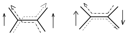
Figure 12: Two paths

If our edges were in two paths $e\in p=(\vec{e}_{1},...,\vec{e}_{n})$ and $e^{\prime}\in p^{\prime}=(\vec{e}^{\prime}_{1},...,\vec{e}^{\prime}_{m})$, then on the new graph $\Gamma_{e,e^{\prime}}$ we would have (formally) two paths $p_{new},p^{\prime}_{new}$.

It is easy to see that

1. $p\neq p^{\prime}\implies p_{new}=p^{\prime}_{new}$;

2. $p=p^{\prime}\implies p_{new}\neq p^{\prime}_{new}$.

By induction one obtains:

1. Any 3-valent graph can be created by a finite chain of such elementary operations starting with the disconnected union of circles $0\cup 0...\cup 0$;

2. every path on $\Gamma$ can be created by a finite chain of elementary operations starting from a path on a disjoint finite set of circles.

These statements give the induction procedure which allows to prove all simple facts about trivalent graphs. There are two types of such problems: Eulerian paths and coloring problems.

Recall that a path $p=(\vec{e}_{1},...,\vec{e}_{n})\in P_{d}(\Gamma)$ is called Eulerian if it contains every oriented edge and exactly one time. A system of paths $P_{E}$ is called Eulerian if every oriented edge is contained and exactly one time in one and exactly one path from this system. Such system is called minimal if $|P_{E}|=min$. This is an invariant of the graph $e(\Gamma)$.

We know already that an elementary operation tranform an Eulerian system $P_{E}$ on $\Gamma$ to the Eulerian system $P^{\prime}_{E}$ on $\Gamma_{e,e^{\prime}}$. Moreover

$$|P^{\prime}_{E}|=|P_{E}|\pm 1.$$

From this it easy to see that for every 3-valent graph $\Gamma$ of genus $g$

1. $1\leq e(\Gamma)\leq g+1$;

2. $e(\Gamma)=g-1mod2$;

3. there exists a chain of elemetary operations with result graph $\Gamma$ such that $e(\Gamma^{\prime})=1$.

We can consider every plane ribbon graph $\Gamma$ as a graph on the plane $\mathbb{R}^{2}$. Such embedded graph defines the geographic map with connected componets of the complement as the countries. This is the 4-colors setup. This problem is stated for embedded graphs.

Other ”coloring” problem for graphs appears in the Feynman diagram technique (for the problem of dependence on the form of Lagrangian and of limits in matrix models). Let $C=(c_{1},...,c_{N})$ is a set of colors. Any coloring is just a map

$$c\colon E(\Gamma)\to C$$

such that for every vertex $v\in V(\Gamma)$ the map $c\colon S(v)\to C$ is an embedding. That is around every vertex all edges have different colors. If the number $N$ of colors is minimal then it is called the chromatic number $N_{min}=\chi(\Gamma)$. Easely we have to consider graphs without 1-loops. Then for 3-valent graphs

$$3\leq\chi(\Gamma)\leq 4.$$

A little more efforts you need to prove the following fact

$\chi(\Gamma)=3$ if and only if there is a set $(l_{1},...,l_{n})$ of disjoint simple loops on $\Gamma$ such that

1. every loop $l_{i}$ contains an even number of edges;

2. for every vertex $v\in V(\Gamma)$ there exists a loop which contains it:

   $$V(\Gamma)\subset\bigcup_{i=1}^{n}l_{i}.$$

Both of these ”coloring” problems are related by the following equivalence: two statements

1. The 4-colors problem admits positive solution;

2. For every plane 3-valent graph $\Gamma$ without 1-loops $\chi(\Gamma)=3$

are equivalent. These problems of ”classical theory” of graphs. Considering every homogeneous graph as a manifold (in style of [BGH]) and following Segal’s ideas we have a reason to consider the ”Loop space” of every graph.

Consider standard interval $[0,1]$ and divide it by a finite set of points to a complex $[0,p_{1},....,p_{d-1},1]$. We can consider this as a 2-valent history with two parabolic edges $[0,p_{1}]$ and $[p_{d-1},1]$. The linking of the parabolic edges of such history gives a cycle (or a loop) that is a closed 2-valent graph.

As we know every continuous combinatorial map

$$p\colon[0,p_{1},....,p_{d-1},1]\to\Gamma$$ (6.34)

is called path of length $d$ in $\Gamma$.

If this path is irreducible, the preimage of every edge

$$p^{-1}(e)=g_{1}\cup...\cup g_{col(e)}$$ (6.35)

is a disjoint union of a finite set of compact 1-graphs and the number of components is equal to $col(e)$ (without any orientation).

Now we consider the set $\mathcal{L}$ of irreducible loops that is closed paths (0=1). The type of loop $l\in\mathcal{L}$ is the non negative function

$$col\colon E(\Gamma)\to\mathbb{Z}_{\geq 0}.$$ (6.36)

(recall that we consider irreducible unmarked loops only).

For any type of loops for every vertex $v\in V(\Gamma)$ with the set of edges $(e_{1,v},e_{2,v},e_{3,v})$ the following constraints hold:

1. $$col(e_{1,v})+col(e_{2,v})+col(e_{3,v})=0\mod 2;$$ (6.37)

2. $$|col(e_{1,v})-col(e_{2,v})|\leq col(e_{3,v})\leq col(e_{1,v})+col(e_{2,v}).$$ (6.38)

Indeed, consider a vertex $v$ and the star $S(v)=e_{1},e_{2},e_{3}$. Let $n_{12}$ be the number equal to how many times we come to $v$ along the edge $e_{1}$ and turn to the edge $e_{2}$. In the same vein we have $n_{ij}$ for every pair of edges from the star. Then

$$col(e_{i})=\sum_{j\neq i}n_{ij}.$$ (6.39)

From this we get the statement immediately.

Now we say that a loop $l\in\mathcal{L}$ has the type of level $k$ if for every edge $e$

$$col(e)\leq k.$$

In the same vein we can prove that the type function (6.36) gives a type of loop of level $k$ iff for every vertex $v\in V(\Gamma)$ with the set of local edges $(e_{1,v},e_{2,v},e_{3,v})$ almost the same constraint holds:

1. $$col(e_{1,v})+col(e_{2,v})+col(e_{3,v})=0mod2;$$

2. and a slightly sophisticated condition 2)

   $$|col(e_{1,v})-col(e_{2,v})|\leq col(e_{3,v})\leq$$ (6.40)

   $$min(col(e_{1,v})+col(e_{2,v}),2k-col(e_{1,v})-col(e_{2,v}).$$

Note that the inequality (6.38) is just the triangle inequality and the inequality (6.40) is the spherical triangle inequality (with $\sqrt{k}$ proportional to the radius of the sphere).

Note also that it is quite reasonable to call every loop as knot.

So every knot defines the type function (6.36) coloring edges of our graph in $\mathbb{Z}_{\geq 0}$ colors. Dividing this function by 2 we get the map

$$1/2col\colon E(\Gamma)\to 1/2\mathbb{Z}_{\geq 0}=\widehat{\operatorname{SU}(2)}$$

where the last set is the set of irreducible representations of $\operatorname{SU}(2)$. Conditions (6.38) and (6.40) mean that any pair $(\Gamma,cal)$ is a $\operatorname{SU}(2)$- spin network.

Recall that to get a marked Riemann surface from a trivalent graph $\Gamma$ we need to pump up our graph, that is, to replace every vertex by a trinion and to glue trinions by tubes along the edges.

6.4 Circle complex and Graph complex

Let $\Sigma_{g,n}$ be an oriented surface of genus $g$ with $n$ punctures and $C$ be a simple, closed, homotopy non-trivial, non-bounded pinchs loop on $\Sigma_{g,n}$. We call such loop a circle and consider it up to the isotopy class.

Circle complex or Curve complex $C(\Sigma_{g,n})$ has the set of circles as 0-skeleton $C_{0}(\Sigma_{g,n})$,

1. 1-skeleton $C_{1}(\Sigma_{g,n})$ is the set of pairs of classes of disjoint circles;

2. triangles correspond to triples of classes of disjoint cirles ;

3. every $i$-simplex corresponds to a set of $i+1$ classes mutually disjoint circles,

4. so, simplexes of maximal dimension are collections of $3g-3$ disjoint circles just as (4.7).

The main fact which we will use is the following: the group of combinatorial automorphisms

$$AutC(\Sigma_{g})=Mod_{g}$$ (6.41)

is the modular group (5.30).

Remark

By the Roiden’s theorem

$$Isom\quad\tau_{g}=Mod_{g}$$ (6.42)

where the Teichmuller space $\tau_{g}$ (5.31) is equipped with the Teichmuller metric. Moreover as a metric space $C(\Sigma_{g,n})$ is very closed to $\tau_{g}$. In particular, $C(\Sigma_{g,n})$ is $\delta$-hyperbolic ([MM]). The same facts are true for the Weil-Peterson metrics.

Recall that in the case of a pinched curve $\Sigma_{g,n}$ the circle can’t be isotopic to a boundary component.

Figure 13: Triangles

For two special but very important cases $\Sigma_{0,4}$ and $\Sigma_{1,1}$ the definition is slightly different (since there are no disjoint pairs of circles ): two vertices are connected by an edge if circles have 2 intersections in $\Sigma_{0,4}$-case and 1 intersection in $\Sigma_{1,1}$-case. In both cases

$$C(\Sigma_{0,4})=C(\Sigma_{1,1})$$ (6.43)

is the ideal triangulation of 2-disc (so called Farey Graph, see Fig. 14).

Figure 14: Farey graph (the ideal triangulation of disk)

Trinion decomposition graph $C_{1}{TD(\Sigma)}$ has the set of trinion decompositions as 0-skeleton

$$V(C_{1}(TD(\Sigma)))=\{(C_{1},...,C_{3g-3})\}$$ (6.44)

(see (4.7)) and a pair of trinion decompositions is connected by an edge if the decompositions differ by an elementary move. That is, in the system of circles $C_{1},\dots,C_{3g-3}$ on a Riemann surface $\Sigma$ we replace only one circle, for example $C_{1}$, with another circle $C^{\prime}_{1}$ intersecting twice if $C_{1}$ and $C^{\prime}_{1}$ don’t lie on the same trinion and intersecting once otherwise (minimal intersections):

$$\{C_{1},\dots,C_{3g-3}\}\to\{C^{\prime}_{1},\dots,C_{3g-3}\}.$$ (6.45)

Recall that every trinion decomposition $C_{1},...,C_{3g-3}$ defines the 3-valent graph $\Gamma$ (4.9)- (4.11). Thus we have the finite graph $C_{1}(TG_{g})$ with the set of vertices

$$V(C_{1}(TG_{g}))=TG_{g}$$

(see (6.21)) and a pair of graphs $\Gamma,\Gamma^{\prime}$ is connected by an edge if they differ by an elementary transformation (see Definition 9) corresponding to an elementary move of trinion decomposition (6.45). The fibers of the map

$$\gamma\colon V(C_{1}(TD(\Sigma)))\to TG_{g}$$

are described by the formula

$$Mod_{g}/AutH_{\Gamma}$$

where $H_{\Gamma}$ is the handlebody (6.9) and $Aut$ is the group of isotopy classes of diffeomorphisms of $\Sigma=\Sigma_{\Gamma}$ extendable to diffeomorphisms of the handlebody.

The finite TG-graph $C_{1}(TG_{g})$ is 1-skeleton of the finite $TG_{g}$-complex $C(TG_{g})$ which can be constructed by the following procedure: first of all let us glue by 2-cells all triangles coming from elementary transformations. Over such triangles in TG-graph we have triangles from Fig. 13 of the infinite TD-graph. Up to such triangles we have the canonical connection $\nabla$ (6.22) on TG-graph and we can apply the ”geodesic technique” (6.25)-(6.28). In particular, we obtain 2-complex $C_{\nabla}(TG_{g})=C(TG_{g})$. The important fact (see Remark at the end of this subsection) proved in [HT] is the following

1. $C(TG_{g})$ is simply connected that is

   $$C(TG_{g})=S^{2},$$

2. hence our TG-graph is plane;

3. hence we may ask about this graph all classical questions, for example, on the chromatic number and so on.

However the standard way to check these properties is the following

1. to construct the infinite complex $C(TD(\Sigma))$ ”by our hands”;

2. to check described properties;

3. to desend all constructions to TG-complex using the map $\gamma:C_{1}(TD)\to C_{1}(TG_{g})$ and to get the complex $C(TG_{g})$;

4. to check the required properties for this finite complex.

Remark

It is quite natural to apply this geodesic technique to the infinite graph $C_{1}(TD(\Sigma))$ directly but we have to go passing the standard way.

For our special cases of Riemann surfaces it can be proved that

$$C_{1}(TD(\Sigma_{0,4}))=C_{1}(TG(\Sigma_{1,2}))=C_{1}(\Sigma_{0,4})=C_{1}(\Sigma_{1,2})$$ (6.46)

is the Farey graph that is 1-skeleton of the Farey complex again.

Figure 15: Squares

The infinite complex $C(TD)$ is 2-dimensional. Its 2-cells represent relations between special moves, that is, loops in $TD$-graph and they can be triangles, squares, pentagones and hexagons. Every trinion decomposition of $\Sigma_{g,n}$ contains trinion decompositions of surfaces with smaller $g$ and $n$ as fragments of it. We call such fragments subsurfaces. The relations, coming from such subsurfaces are the following:

Figure 16: Pentagons

1. $\Sigma_{1,1}$ and $\Sigma_{0,4}$ for triangles;

2. $$\Sigma_{1,1}\cup\Sigma_{0,4}=\Sigma_{1,3}$$ (6.47)

   for squares;

3. $\Sigma_{0,5}$ for pentagons and

4. $\Sigma_{1,2}$ for hexagons

(see Figures 13, 15-17).

Figure 17: Hexagons

Amazing fact is that we can define 2-cells of this complex in terms of $TD$-graph. It means that $C(TD)$-complex carries no more information than its 1-skeleton:

1. triangles are contained in subcomplexes $C(TD(\Sigma_{1,1}))$ or $C(TD(\Sigma_{0,4}))$ which are the Farey complexes. Every edge of this complex is a side of two triangles corresponding to two subsurfaces $C(TD(\Sigma_{1,1}))$ or $C(TD(\Sigma_{0,4}))$;

2. moreover, if we fix one vertex in any Farey subgraph of $TGD$-graph, we get a circle which is a vertex of $C(\Sigma_{g,n})$ (indeed, fixing any Farey subgraph of $TD$-graph we get the collection $\{C_{1},\dots,C_{3g-3}\}$ of circles of trinion decompositions with fixed set of circles $(C_{2},\dots,C_{3g-3})$, since our Farey subgraph corresponds to a choice of $C_{1}$ );

3. if $C$ is a vertex of $C(\Sigma)$ (as $C_{1}$ before ) then there exists a Farey subgraph with fixed vertex but not unique (indeed we can extend our circle $C_{1}$ to a complete set $\{C_{1},\dots,C_{3g-3}\}$ and consider all trinion decompositions with fixed $(C_{2},\dots,C_{3g-3})$; we get a Farey subgraph $F_{C}$ (just a possible choice) with fixed point $p\in F_{C}$);

4. now we can define a map

   $$\phi\colon AutC_{1}(TD)\to AutC_{0}(\Sigma_{g,n})$$ (6.48)

   sending a circle $C\in C_{0}(\Sigma_{g,n})$ to unique vertex in $C_{0}(\Sigma_{g,n})$ corresponding to the marked Farey graph $g(p)\in g(F_{C})$;

5. square, pentagon or hexagon ($n$-gones for small $n$) can be union of triangle and $n-1$-gon gluied along an edge. To distinguish this trivial situation from ”non trivial” or alternating we consider a loop with $n$ consecutive points such that every consecutive triple $p_{i},p_{i+1},p_{i+2}$ and the pair of edges between arn’t contained in any Farey subcomplex;

6. at last, a hexagon can be almost alternating when its three consecutive vertices can be extended to the set of vertices of a square loop.

Using these simple rules Margalit proved in [M] that

1. the map $\phi$ (6.47) can be extended to a well defined map

   $$AutC_{1}(TD)\to AutC(TD),$$ (6.49)

2. and this map can be extended to an isomorphism

   $$\phi\colon AutC(TD)\to AutC(\Sigma),$$ (6.50)

3. such that

   $$AutC_{1}(TD)=AutC(TD)=AutC(\Sigma)=Mod_{g}.$$ (6.51)

TD-complex $C(TD)$ was introduced by Hatcher and Thurston in [HT] where they proved that this complex is connected and simple connected. But the equality (6.50) was proved quite recently in [M].

Remark

Returning to the Rational Conformal Field Theory WZW we can consider the vector space spanned by different conformal blocks (see Definition 8) interpreted as the holomorphic sections of some power of theta-line bundle on the moduli space of semi-stable vector bundles on a Riemann surface $\Sigma$ (see section 3). This surface can be formed by gluing a number of trinions. The conformal blocks are obtained by summing over the intermediate states passing through the circles along which we glue our trinions. Different gluing procedures lead to different bases of the same vector space. Hence vectors of this space obtained by one gluing procedure can be expressed as linear combinations of vectors found by another way of gluing the same surface. These linear transformations are given by dual matrices, which have to satisfy some consistency conditions. To describe these conditions it is quite convinient to use the finite complex $C(TG)$. First of all, we have some very simple duality matrices defined by the elementary moves. The complex $C(TG)$ is connected, hence every duality matrix can be represented as a product of the simple ones (maybe not uniquely). To get an unambiguous description of all duality matrices, we have to use consistency conditions on simple duality matrices which are given by loops of simple matrices. So we have to find all independent conditions. Every loop of simple matrices corresponds to the statement that the product of the corresponding duality matrices is equal to one. Fixing a collection of fundamental loops, like triangles, squares , pentagons and hexagons before, and filling faces of such loops gives us the graphs complex $C(TG)$. The relations for the loops are complete iff the complex is simply connected. Thus we get a system of (polynomial) equations for duality matrices. Solutions to this system of equations give the moduli space of rational conformal field theories. Sending the level $k$ to infinity we get a fusion algebra which for our $\operatorname{SU}(2)$-case is the representation algebra $R(sl(2,\mathbb{C}))$ from subsection 5.1.

Returning to wave function spaces $\mathcal{H}^{k}_{\Gamma}$ (4.43) we will see that the system of these spaces defines a vector bundle

$$\mathcal{H}^{k}_{TG}\to C(TG_{g})=S^{2}$$ (6.52)

on the $TG$- complex with a special structure-some local linear decomposition on line subbundles.

Remark that the bundles is a subbundle of the trivial bundle (see (4.45))

$$\mathcal{H}^{k}_{TG}\subset\mathbb{C}^{(2k)^{3g-3}}\times C_{TG}=(\oplus_{\alpha\in T^{A}_{2k}}\mathbb{C}_{\alpha})\times C_{TG}.$$ (6.53)

All these constructions suggest existence of a flat connection $a_{K}$. Since the complex $C_{TG}$ is simply connected the bundle $\mathcal{H}^{k}_{TG}$ has to be trivial with the trivialization defined up to scaling. From this we get the projective bundle

$$\mathbb{P}\mathcal{H}^{k}\to\mathcal{M}_{g}$$ (6.54)

on the moduli space of curves of genus $g$ with the projective flat connection. But this bundle is a slight projective bundle with the phase amplitude (6.18) only.

Returning to the graph $C^{1}_{TG_{g}}$ we will see that

1. the system of duality matrices defines a flat connection on $C_{1}(TG_{g})$;

2. this connection has trivial projective monodromy, thus

3. this connection defines a representation

   $$\rho\colon AutC_{1}(TG_{g})\to PGL(rk_{g}(\emptyset)),\mathbb{C}).$$ (6.55)

4. this representation is equal to the desired Kohno representation.

6.5 Gauge theory on graphs.

A connection $a$ on the trivial $\operatorname{SU}(2)$-bundle on $\Gamma$ is a map

$$a\colon P_{1}(\Gamma)\to\operatorname{SU}(2)$$ (6.56)

such that for the orientation reversing involution $i_{e}$ we have

$$a(i_{e}(\vec{e}))=a(\vec{e})^{-1}.$$ (6.57)

Then the “path integral” is

$$a((\vec{e}_{1},\dots,\vec{e}_{d}))=a(\vec{e}_{1})\cdot\cdots\cdot a(\vec{e}_{d})\in\operatorname{SU}(2)$$ (6.58)

that is, it is the map

$$a\colon P_{d}(\Gamma)\to\operatorname{SU}(2)$$ (6.59)

such that for the orientation reversing involution $i_{\Delta}$ we have

$$a(i((\vec{e}_{1},\dots,\vec{e}_{d})))=a((\vec{e}_{1},\dots,\vec{e}_{d}))^{-1}.$$ (6.60)

In the same vein we have the monodromy map for loops

$$a\colon L_{d}(\Gamma)_{v}\to\operatorname{SU}(2).$$ (6.61)

Obviously every such connection is flat .

Let $\mathcal{A}(\Gamma)$ be the space of connections that is the space of functions (6.56) subjecting to the constraint (6.57):

$$\mathcal{A}(\Gamma)=\{a\in\operatorname{SU}(2)^{P_{1}(\Gamma)}|a(i_{e}(\vec{e}))=a(\vec{e})^{-1}\}.$$ (6.62)

Every element $\widetilde{g}$ of the gauge transformations group $\mathcal{G}(\Gamma)$ is a function

$$\widetilde{g}\colon V(\Gamma)\to\operatorname{SU}(2)$$ (6.63)

that is

$$\mathcal{G}(\Gamma)=\operatorname{SU}(2)^{V(\Gamma)}$$ (6.64)

with the componentwise multiplication.

This group acts on the space of connections $\mathcal{A}(\Gamma)$ by the following rule

$$\widetilde{g}(a(\vec{e}))=\widetilde{g}(v_{s}(\vec{e}))\cdot a(\vec{e})\cdot\widetilde{g}(v_{t}(i(\vec{e}))).$$ (6.65)

Recall that $\widetilde{g}(v_{t}(i(\vec{e})))=\widetilde{g}(v_{t}(\vec{e}))^{-1}.$

The space of gauge orbits

$$\mathcal{B}(\Gamma)=\mathcal{A}(\Gamma)/\mathcal{G}(\Gamma)$$ (6.66)

is the space of classes of representations of the fundamental group of $\Gamma$ as it is expected because all our connections are flat:

$$\mathcal{A}(\Gamma)/\mathcal{G}(\Gamma)=CLRep(\pi_{1}(\Gamma),\operatorname{SU}(2))$$ (6.67)

is the quotient of the space of representations by the adjoint action

$$CLRep(\pi_{1}(\Gamma),\operatorname{SU}(2))=\operatorname{Hom}(\pi_{1}(\Gamma),\operatorname{SU}(2))/Ad\operatorname{SU}(2)$$ (6.68)

- the space of classes of representations of this group.

Obviously the fundamental group of 3-valent graph $\Gamma$ of genus $g$ is the free group with $g$ generators. Thus the quotient (6.66)

$$CLRep(\pi_{1}(\Gamma),\operatorname{SU}(2))=uS_{g}$$ (6.69)

is the unitary Schottki space. (see the definition (4) in 3.2 after the formula (3.44)).

The gauge transformation group $\mathcal{G}(\Gamma)$ contains the diagonal subgroup

$$\operatorname{SU}(2)_{\Delta}\subset\mathcal{G}(\Gamma)$$ (6.70)

of constant functions (6.63). The action of this subgroup defines the space of constant orbits

$$CL\mathcal{A}(\Gamma)=\mathcal{A}(\Gamma)/\operatorname{SU}(2)_{\Delta}.$$ (6.71)

For every vertex $v\in V(\Gamma)$ we have the subgroup

$$\mathcal{G}(\Gamma)_{v}=\{\widetilde{g}\in\mathcal{G}(\Gamma)|\widetilde{g}(v)=\operatorname{id}\}$$ (6.72)

of gauge transformations preserving the framing at $v$. This is a normal subgroup, and

$$\mathcal{G}(\Gamma)/\mathcal{G}(\Gamma)_{v}=\operatorname{SU}(2)_{\Delta}$$ (6.73)

Thus the full group of gauge transformations is a semidirect product of $\mathcal{G}(\Gamma)_{v}$ and $\operatorname{SU}(2)_{\Delta}$.

The quotient

$$\mathcal{A}(\Gamma)/\mathcal{G}(\Gamma)_{v}=Rep(\pi_{1}(\Gamma,v),\operatorname{SU}(2))$$ (6.74)

is the orbit space of framed (at $v$) connections. This space depends on the choice of a point $v$.

Thus the quotient map (6.67)

$$P\colon\mathcal{A}(\Gamma)\to CLRep(\pi_{1}(\Gamma),\operatorname{SU}(2))$$ (6.75)

can be decomposed as follows

$$\mathcal{A}(\Gamma)\xrightarrow{\,P\,}Rep(\pi_{1}(\Gamma),\operatorname{SU}(2))\xrightarrow{/\operatorname{SU}(2)\Delta}CLRep(\pi_{1}(\Gamma),\operatorname{SU}(2))$$ (6.76)

or

$$\mathcal{A}(\Gamma)\xrightarrow{/\operatorname{SU}(2)_{\Delta}}CL\mathcal{A}(\Gamma)\xrightarrow{P_{cl}}CLRep(\pi_{1}(\Gamma),\operatorname{SU}(2)).$$ (6.77)

The involution $i_{\Delta}$ acts on the space $\mathcal{A}(\Gamma)$ of connections

$$i^{*}_{\Delta}\colon\mathcal{A}(\Gamma)\to\mathcal{A}(\Gamma)$$ (6.78)

and there exists an element

$$\widetilde{g}_{i}=\begin{pmatrix}0&1\\ -1&0\end{pmatrix}\in\operatorname{SU}(2)_{\Delta}\subset\mathcal{G}(\Gamma)$$ (6.79)

such that

$$i^{*}_{\Delta}=\widetilde{g}_{i}.$$ (6.80)

Thus the involution $i^{*}_{\Delta}$ (3.23) acts trivially on $CL\mathcal{A}(\Gamma)$. Recall that a gauge fixing is a section of the projection $P$ (6.75).

Recall that the set $\operatorname{Conj}(\operatorname{SU}(2))$ of conjugacy classes of elements of $\operatorname{SU}(2)$ can be described as the interval $[0,1]$ with respect to the map

$$conj\colon\operatorname{SU}(2)\to\operatorname{Conj}(\operatorname{SU}(2))=[0,1]$$ (6.81)

sending a matrix $g\in\operatorname{SU}(2)$ to

$$conjg=\frac{1}{\pi}\cdot\cos^{-1}\Bigl{(}\frac{1}{2}\operatorname{Tr}g\Bigr{)}\in[0,1].$$ (6.82)

Using this map coordinatewise one obtains the map

$$conj\colon\operatorname{CL}\mathcal{A}(\Gamma)\to[0,1]^{3g-3}=\prod_{e\in E(\Gamma)}[0,1]_{e},$$ (6.83)

which is obviously surjective.

The map $conj$ is the composite

$$\mathcal{A}(\Gamma)\xrightarrow{\operatorname{SU}(2)_{\Delta}}\operatorname{CL}\mathcal{A}(\Gamma)\to[0,1]^{3g-3}=\prod_{e\in E(\Gamma)}[0,1]_{e}$$ (6.84)

and the involution $i_{\Delta}$ preserves its fibers.

6.6 Abelian gauge theory and $U(1)$-spin networks

Abelian gauge theory on $\Gamma$ is a good model for non-Abelian gauge theory. Abelian spin networks can be considered as theta-characteristics under numeration of theta functions. A $U(1)$-connection $a$ is a map

$$a\colon P_{1}(\Gamma)\to U(1)$$ (6.85)

such that

$$a(i_{e}(\vec{e}))=a(\vec{e})^{-1}.$$ (6.86)

The “path integral” is given by

$$a((\vec{e}_{1},\dots,\vec{e}_{d}))=\prod_{\vec{e}\in P_{1}(\Gamma)}a(\vec{e})\in U(1),$$ (6.87)

and so on. Again let

$$\mathcal{A}_{U(1)}(\Gamma)=\bigl{\{}a\in U(1)^{P_{1}(\Gamma)}\bigm{|}a(i_{e}(\vec{e}))=a(\vec{e})^{-1}\bigr{\}}.$$ (6.88)

be the space of $U(1)$-connections. Then we have the same involution

$$\mathcal{A}_{U(1)}(\Gamma)\xrightarrow{i^{*}_{e}}\mathcal{A}_{U(1)}(\Gamma).$$ (6.89)

Every element $\widetilde{u}$ of the gauge transformation group $\mathcal{G}_{U(1)}(\Gamma)$ is a function

$$\widetilde{u}\colon V(\Gamma)\to U(1).$$ (6.90)

This group acts on the space of connections $\mathcal{A}_{U(1)}(\Gamma)$ by the same rule:

$$\widetilde{u}(a(\vec{e}))=\widetilde{u}(v_{s}(\vec{e}))\cdot a(\vec{e})\cdot\widetilde{u}(v_{t}(i(\vec{e}))).$$ (6.91)

However, there is one important difference between Abelian and non-Abelian theories. Namely, the diagonal group

$$U(1)_{\Delta}\subset\mathcal{G}_{U(1)}(\Gamma)$$ (6.92)

has trivial action. Thus

$$\mathcal{B}_{U(1)}(\Gamma)=\mathcal{A}_{U(1)}(\Gamma)/\mathcal{G}_{U(1)}(\Gamma)=\operatorname{Hom}(\pi_{1}(\Gamma),U(1))=U(1)^{g}.$$ (6.93)

Remark that this is abelian unitary Schottki space, that is, the zero fiber of the projection $\pi$ (2.22) on which we are constructing our delta functions (2.46) and (2.48) for the application of the coherent state transform to get an analytical presentation of theta functions on the complex Schottki space $(\mathbb{C}^{*})^{g}$. We would like to do this for non-abelian case too.

Let

$$P_{a}\colon\mathcal{A}_{U(1)}(\Gamma)\to U(1)^{g}$$ (6.94)

be the projection map.

The abelian and non-abelian theories are related by the following map:

$$d\colon\mathcal{A}_{U(1)}(\Gamma)\to\mathcal{A}(\Gamma)\quad\hbox{given by}\quad d(a(\vec{e}))=\begin{pmatrix}e^{i\phi},0\\ 0,e^{-i\phi}\end{pmatrix}.$$ (6.95)

This map $d$ is equivariant with respect to every involution $i^{*}_{e}$. Obviously the image $d(\mathcal{A}_{U(1)}(\Gamma))\subset\mathcal{A}(\Gamma)$ is a 2-section of the projection $conj$, that is, the composite

$$conj\circ d\colon\mathcal{A}_{U(1)}(\Gamma)\to\prod_{e\in E(\Gamma)}[0,1]_{e}$$ (6.96)

is the factorization by the involution $i^{*}_{\Delta}$.

It is easy to check

Proposition 23

In the chain of maps

$$\mathcal{A}_{U(1)}(\Gamma)\xrightarrow{\,d\,}\mathcal{A}(\Gamma)\xrightarrow{\,P\,}U(1)^{g}\in\mathrm{CLRep}(\pi_{1}(\Gamma))$$ (6.97)

the composite $d\circ P$ is the projection map $P_{a}$ (5.75).

The set of irreducible representations of $U(1)$ is

$$\widehat{U(1)}=\mathbb{Z}$$ (6.98)

and a spin $U(1)$-network on a graph $\Gamma$ is given by a function

$$w\colon E(\Gamma)\to\widehat{U(1)}=\mathbb{Z}$$ (6.99)

(like (4.46)) such that for every triple of edges meeting at a vertex $v\in V(\Gamma)$ the following condition holds

$$w(e_{1})+w(e_{2})+w(e_{3})=0.$$ (6.100)

Thus the triangle inequality (Clebsh-Gordan conditions) becomes the equality.

Again a spin network is of level $k$ when $w(e)\leq 2k$.

Considering the basis $(a_{1},\dots,a_{g},b_{1},\dots b_{g})$ (2.32) we have the decomposition of the jacobian of the curve $\Sigma_{\Gamma}$

$$J_{\Sigma_{\Gamma}}=Hom(\pi_{1}(\Sigma_{\Gamma}),U(1))=\prod_{i=1}^{g}U(1)_{a_{i}}\times\prod_{i=1}^{g}U(1)_{b_{i}}$$ (6.101)

which coincides with the decomposition (2.21),(2.32).

Now we can consider the coordinates (4.14) of the map (4.41) as elements of the target group $U(1)$. Hence the map $\pi_{\Gamma}$ (4.41) has the form

$$\pi_{\Gamma}\colon J_{\Sigma_{\Gamma}}\to U(1)^{E(\Gamma)}=T^{A}$$ (6.102)

where the target is the action torus (4.40). The image of this map is a g-dimensional torus

$$\Delta_{\Gamma}=T^{g}_{-}\subset T^{A}.$$ (6.103)

Now we can send every spin network that is a function (6.98) satisfying (6.99) to a point of order $k$ on $T^{A}$ dividing by $k$

$$w(e)\to 1/kw(e).$$ (6.104)

We get the map of the set $SNW_{a}^{k}$ of abelian spin works of level $k$

$$1/k\colon SNW_{a}^{k}\to(T^{A})_{k}.$$ (6.105)

Amusing fact is that

$$1/k(SNW_{a}^{k})\subset\Delta_{\Gamma}=T^{g}_{-}.$$ (6.106)

Moreover

$$1/k(SNW_{a}^{k})=W^{k}(\Gamma)=BS_{k}(\Gamma).$$ (6.107)

Thus we get the canonical identification of the set $\mathbb{Z}^{g}/k\mathbb{Z}^{g}$ of theta characteristics of level $k$ (2.48) with the set of spin networks

$$(\mathbb{Z}^{g}/k\mathbb{Z}^{g})=SNW_{a}^{k}.$$ (6.108)

So in the classical case we can use $U(1)$-spine networks for the enumeration of theta characteristics. In the same vein we will use $\operatorname{SU}(2)$-spin networks for the enumeration of non-abelian theta characteristics.

Also we saw that the harmonic analysis on $T^{g}_{+}=U(1)^{g}$ is the standard Fourier analysis on a torus. We use the Fourier decomposition to define our delta-functions (2.46) and (2.48) which CST $C_{t}^{-i\Omega}$ (2.42) sends to classical theta functions. Now we have to extend these constructions to the non-abelian case.

6.7 Harmonic analysis of $\operatorname{SU}(2)$-spin networks

Recall that a spin network defines a map $j\colon E(\Gamma)\to\widehat{SU(2)}$ with constraints. For a triple of representations $j_{e_{1}},j_{e_{2}},j_{e_{3}}$ an intertwiner is trivial component of the tensor product $j_{1}\otimes j_{2}\otimes j_{3}$. Such a component exists iff under the traditional identification $\widehat{SU(2)}=\textstyle\frac{1}{2}\mathbb{Z}^{+}$ the Clebsch–Gordan conditions

$$j_{1}+j_{2}+j_{3}\in\mathbb{Z}\quad\text{and}\quad|j_{1}-j_{2}|\leq j_{3}\leq j_{1}+j_{2}$$ (6.109)

(the triangle inequality) hold. Function $j\colon E(\Gamma)\to\widehat{SU(2)}$ defines a spin network $\Gamma_{j}$ iff these conditions hold for every triple $j_{v,1},j_{v,2},j_{v,3}$ of representations around every vertex $v\in V(\Gamma)$.

Any intertwiner $i_{v}\in j_{v,1}\otimes j_{v,2}\otimes j_{v,3}$ is defined uniquely so one omits any labeling of the vertices and denotes $\operatorname{SU}(2))$-spin network by the symbol $\Gamma_{j}$.

Spin network $\Gamma_{j}$ is of level $k$ if $j_{i}\leq k$ for every edge $e_{i}$ and in the last inequality we take $min(j_{1}+j_{2},k-j_{1}-j_{2})$ instead of $j_{1}+j_{2}$. Of course if $k^{\prime}>k$ then every spin network of level $k$ is of level $k^{\prime}$ automatically. We would like to fix a level and denote a spin network of level $k$ by the symbol $\Gamma_{j^{k}}$ and the set of all spin net works by the symbol $SNW^{k}(\Gamma)$. Recall that we have the identification $SNW^{k}(\Gamma)=W^{k}(\Gamma)$ (see the end of subsection 6.1).

Spin network $\Gamma_{j,k}$ is a purely combinatorial object but we can identify it with a function on the special space - the unitary Schottky space $uS_{g}$ given by the formula

$$uS_{g}=\operatorname{SU}(2)^{g}/Ad_{\mathrm{diag}}\operatorname{SU}(2)$$ (6.110)

where $Ad_{\mathrm{diag}}\operatorname{SU}(2)$ is the diagonal adjoint action on the direct product. This space doesn’t depend on a three valent graph modulo the choice of appropriate topological data. Only one invariant of a graph is used, namely its genus $g$.However, it is quite natural to use a graph $\Gamma$ as a starting point of the construction.

Consider the product

$$\operatorname{SU}(2)^{E(\Gamma)}=\prod_{e\in E(\Gamma)}\operatorname{SU}(2)_{e}$$ (6.111)

with $\operatorname{SU}(2)$ components enumerated by edges of $\Gamma$ which we can identify with the space of flat connections $\mathcal{A}$ (6.88) (under a choice of any orientation of $\Gamma$).

Let $dx$ be the Haar measure on $\operatorname{SU}(2)$ normalized by the condition $\int_{\operatorname{SU}(2)}dx=1$ and $\vec{d}x$ the product measure on $\operatorname{SU}(2)^{E(\Gamma)}$ normalized by $\int\vec{d}x=1$. Then by the Peter–Weyl formula, any function $f\in L^{2}(\operatorname{SU}(2)^{E(\Gamma)},\vec{d}x)$ has the decomposition

$$f(x)=\sum_{\vec{\rho}\in\widehat{\operatorname{SU}(2)^{E(\Gamma)}}}\operatorname{Tr}[B_{\vec{\rho},f}\vec{\rho}(x)],$$ (6.112)

where $\widehat{\operatorname{SU}(2)^{E(\Gamma)}}$ is the space of irreducible representations of $\operatorname{SU}(2)^{E(\Gamma)}$, and $B_{\vec{\rho},f}$ are endomorphisms of the space $V_{\vec{\rho}}$ of the representation $\vec{\rho}$, given by

$$B_{\vec{\rho},f}=\frac{1}{\dim V_{\vec{\rho}}}\int_{\operatorname{SU}(2)^{E(\Gamma)}}f(x)\vec{\rho}\,^{-1}(x)\vec{d}x.$$ (6.113)

Every irreducible representation of $\operatorname{SU}(2)^{E(\Gamma)}$ is given by tensor product of irreducible representations of $\operatorname{SU}(2)$ $\vec{\rho}=\rho_{1}\otimes\cdots\otimes\rho_{3g-3}$. So every spin network $\Gamma_{j}$ of genus $g$ defines a representation of $\operatorname{SU}(2)^{E(\Gamma)}$ by the tensor product of all labels $\vec{j}=\bigotimes_{e\in E(\Gamma)}j_{e}$.

Of course this is an analog of the standard Fourier decomposition (2.41) or even (2.46). Here the representation $\vec{\rho}$ is a label of frequency and an endomorphism $B_{\vec{\rho},f}$ is the Fourier coefficient that is the analog of a number. The formula (6.113) is nothing else than the integral formula for a Fourier coefficient.

Every endomorphism of the space $V_{\vec{j}}$ is a vector in the tensor product

$$\Bigl{(}\bigotimes_{e\in E(\Gamma)}j_{e}\Bigr{)}\otimes\Bigl{(}\bigotimes_{e\in E(\Gamma)}j_{e}\Bigr{)}^{*}=\Bigl{(}\bigotimes_{e\in E(\Gamma)}j_{e}\Bigr{)}\otimes\Bigl{(}\bigotimes_{e\in E(\Gamma)}j_{e}\Bigr{)},$$

since we are dealing with $\operatorname{SU}(2)$-representations.

But after symmetrizing components of the final product can be labeled by elements of the set $F(\Gamma)$, and we can decompose it as

$$\Bigl{(}\bigotimes_{e\in E(\Gamma)}j_{e}\Bigr{)}\otimes\Bigl{(}\bigotimes_{e\in E(\Gamma)}j_{e}\Bigr{)}^{*}=\bigotimes_{v\in V(\Gamma)}(j_{v,1}\otimes j_{v,2}\otimes j_{v,3}).$$ (6.114)

For every triple of representations around a vertex $v\in V(\Gamma)$ we have a vector $i_{v}\in j_{v,1}\otimes j_{v,2}\otimes j_{v,3}$ and their tensor product gives us the vector

$$B(\Gamma_{j})=\bigotimes_{v\in V(\Gamma)}i_{v}\in EndV_{\vec{j}}\,.$$ (6.115)

So one has the function

$$f_{\Gamma_{j}}(x)=Tr[B(\Gamma_{j})\vec{j}(x)]\in L^{2}(\operatorname{SU}(2)^{E(\Gamma)},d\vec{x}).$$ (6.116)

This function is invariant with respect to the action on $\operatorname{SU}(2)^{E(\Gamma)}=\mathcal{A}$ of the gauge group on $\Gamma$ $\operatorname{SU}(2)^{V(\Gamma)}=\prod_{v\in V(\Gamma)}\operatorname{SU}(2)_{v}$ with components enumerated by the vertices and an orientation of $\Gamma$.

It is easy to see that the endomorphism $B(\Gamma_{j})$ (5.96) is an intertwiner with respect to such action. Then by the standard result of harmonic analysis on groups our function $f_{\Gamma_{j}}$ is invariant with respect to this action. That is, $f_{\Gamma_{j}}$ is a function on the homogeneous space

$$uS_{g}=\mathcal{A}/\mathcal{G}.$$ (6.117)

But the set $\{\Gamma_{j}\}=SNW^{k}(\Gamma)=W^{k}(\Gamma)$ enumerates the collection of functions $f_{\Gamma_{j}}$ (6.115) each of which is an analog of the function (2.48) enumerated by the set $(\mathbb{Z}^{g}/k\mathbb{Z}^{g})$ of theta characteristics.

Proposition 24

Graph $\Gamma$ and function $f_{\Gamma_{j}}$ determine spin network $\Gamma_{j}$ uniquely.

Indeed,

1. knowing graph we can reconstruct the map $P\colon\mathcal{A}\to uS_{g}$;

2. lifting function $f\Gamma_{j}$ on $\mathcal{A}=\operatorname{SU}(2)^{E(\Gamma)}$ and using the harmonic decomposition of this function on $\mathcal{A}$ (6.61) we determine the representation $j_{1}\otimes\dots\otimes j_{3g-3}$ and the space $V$ of this representation;

3. by the Peter-Weyl formula we determine the endomorphism $B(\Gamma_{j})$ (6.114);

4. decomposing this endomorphism on blocks (6.113) correspoding to vertices we reconstruct the function $j$ (6.4).

and we are done.

Now we are ready to construct CST for the pair $uS_{g}\subset S_{g}$ (see the end of 3.2) since the complex Schottki space $S_{g}$ is the complexification of $uS_{g}$.

6.8 RCFT and Kohno representation

The usual data for RCFT include an algebra $A$ and a discrete set $R$ of representations (a finite set for level $k$) $\{\rho_{i}\}$ (just like in subsection 5.1) such that

$$\rho\in R\implies\rho^{*}\in R,$$ (6.118)

and a distinguished element $1$ such that $1^{*}=1$. Moreover for every ordered triple $\rho_{i},\rho_{j},\rho_{k}$ we have a finite (rationality of RQFT) dimensional space $V^{\rho_{i}}_{\rho_{j},\rho_{k}}$.

$$dimV^{1}_{\rho_{i},\rho_{j}}=1\quad\text{ if }\quad\rho_{i}=\rho_{j}^{*}$$ (6.119)

and 0 otherwise.

Remark

So we can extract a modular tensor category from RCFT.

Having such $RCFT$ and 3-1-valent graph $\Gamma$ and a spin network $\Gamma_{j}$ we get from every vertex $v\in V(\Gamma)$ the spaces with edges $e_{1},e_{2},e_{3}$ through it thus we have the space of intertwiners

$$V^{j_{1}}_{j_{2},j_{3}}\in j_{1}\otimes j_{2}\otimes j_{3}$$ (6.120)

(like in (6.6)). Taking tensor products of them together over all vertices we get the space

$$\mathcal{H}^{k}_{\Gamma_{j}}=\otimes_{v\in V(\Gamma)}V^{j_{1}}_{j_{2},j_{3}}$$ (6.121)

and taking a direct product over all possible networks (labelings) we get the space

$$\mathcal{H}^{k}_{\Gamma}=\oplus_{j\in SNW^{k}(\Gamma)}\mathcal{H}^{k}_{\Gamma_{j}}.$$ (6.122)

For $\operatorname{SU}(2)$-case we have

1. $dimV^{j_{1}}_{j_{2},j_{3}}=1$;

2. $dim\mathcal{H}^{k}_{\Gamma_{j}}=1$;

3. the space (6.121) is precisely our space (4.39), (4.43) of wave functions under Bohr-Sommerfeld quantization.

It is useful to fix bases in all our spaces. (In $\operatorname{SU}(2)$-case where all spaces are 1-dimensional we can do it using the standard Wigner 3j-symbols (for recalling and quantum groups extention see [KR]). We equipe the wave function spaces with bases.

This construction hasn’t to be invariant with respect to changes in trinion decompositions (or changes of bases). But having the complex $TG_{g}$ we know the obstackles.

To get such invariance we have to produce matrices of transformations to new bases and check that these matrices satisfy the same algebraic identities as the changes of decompositions themselves. We have to check that these matrices satisfy the same algbraic equations as our transformations itselves (see Fig.11, Definition 9 and 1)-4) around (6.47)).

Fortunately there are 5 elementary moves only described in [MS] with traditional symbols

$$F,\quad S,\quad,T,\quad,\Omega,\quad,\Theta$$ (6.123)

satisfying the required algebraic relations.

Recall that elementary transformations of 3-valent graphs admit relations 1)-4) around (6.47). So our intertwiners vector spaces must satisfy the system of identities described below:

1. 3 transformations are diagonal matrices of phases (6.18) (in an appropriate basis)

   $$\Omega^{\pm},\quad\Theta,\quad T\colon V^{\rho_{i}}_{\rho_{j},\rho_{k}}\to V^{\rho_{i}}_{\rho_{j},\rho_{k}};$$ (6.124)

2. ”genus 1 equality ”

   $$S\colon V^{\rho_{i}}_{\rho_{j},\rho_{j}^{*}}\to\sum_{l}V^{\rho_{i}}_{\rho_{l},\rho_{l}^{*}};$$ (6.125)

3. the fusing matrix

   $$F\colon V^{\rho_{i}}_{\rho_{j},\rho_{k}}\otimes V^{\rho_{k}}_{\rho_{t},\rho_{m}}\to\sum_{l}V^{\rho_{j}}_{\rho_{t},\rho_{l}}\otimes V^{\rho_{l}}_{\rho_{j},\rho_{m}};$$ (6.126)

4. the braiding matrix

   $$B^{\pm}=F\Omega^{\pm}F^{-1}$$ (6.127)

   subjecting the ordinary Reidemeister relations

   $$B_{12}B_{23}B_{12}=B_{23}B_{12}B_{23}.$$ (6.128)

We can see that the most general topological (geometrical) setting for applying of discussed TQFT is a 3-manifold containing a 3-valent graph (instead a loop = knot). So the most striking difference between such objects and spin networks is following: in spin networks the holonomy of one edge around another is trivial that is any ”braiding” relations are absent. In spin networks it isn’t necessary to distinguish over and under crossing when a 3-valent graph is projected on a plane. Otherwise all rules for evaluating spin networks closely parallel the skein rules for the Jones polynomials. Here we are translating RCFT setting to Penrose’s interpretation of the quantum gravity.

Recall that all braid properties of all matrices in the game are arising from the holonomy of the Knizhnik-Zamolodchikov equation (see [KZ]) and the polynimial equations for these matrices expected from the Conformal Field Theory were proposed by Moore and Seiberg in [MS].

Consider a 1-3-valent graph $\Gamma$ which corresponds to a trinion decomposition of a pinched Riemann sphere $\Sigma=\mathbb{P}^{1}-p_{1}-\dots-p_{n}$.

Let

$$\{I_{\mu}\},\quad\mu=1,2,3$$ (6.129)

be any orthonormal basis of $sl(2,\mathbb{C})$ with respect to the Cartan-Killing form and

$$\Omega=\sum_{\mu}I_{\mu}\otimes I_{\mu}\in End(1)=End(sl(2,\mathbb{C})).$$ (6.130)

Let $\pi_{i}(I_{\mu})$ be the action on i-th component of the tensor product $j_{1}\otimes\dots\otimes j_{n}$ (of some labeling of the graph) and

$$\Omega_{ij}=\sum_{\mu}\pi_{i}(I_{\mu})\pi_{j}(I_{\mu})\in End(j_{1}\otimes\dots\otimes j_{n}).$$ (6.131)

Consider the configuration space

$$\mathbb{C}^{n}-\Delta=\{(z_{1},\dots,z_{n})|i\neq j\implies z_{i}\neq z_{j}\}$$ (6.132)

and the trivial vector bundle on it with the fiber $j_{1}\otimes\dots\otimes j_{n}$. It is easy to check that the KZ-equation

$$\partial\Phi/\partial z_{i}=\frac{1}{k+2}\sum_{i\neq j}\frac{\Omega_{ij}}{z_{i}-z_{j}}\Phi,\quad 1\leq i\leq n$$ (6.133)

defines a slightly projective flat connection

$$\omega=\frac{1}{k+2}\sum_{i<j}\Omega_{ij}dlog(z_{i}-z_{j})$$ (6.134)

on this trivial bundle. Any solution of the KZ-equation gives a covariant constant (horizontal) section of this bundle.

Using the detailed information on the monodromy of this equation Tsuchiya and Kanie proposed the operator formalism two dimensional conformal field theory in [TK]. We can use this information too but we would like to present the matrices of MS-axiomatic description in more background independent way.

First of all consider the sphere with 4 holes $\Sigma_{0,4}$ and two graphs $\Gamma$ and $\Gamma^{\prime}_{e}$ corresponding to two types of trinion decompositions of it (see Fig.11).

Symbolically we can note every labeling of $\Gamma$ by the matrix

$$\begin{pmatrix}j_{2}&&&&j_{3}\\ &&j&&\\ j_{1}&&&&j_{4}\end{pmatrix}$$ (6.135)

Then for the graph $\Gamma^{\prime}_{e}$ the matrix has the form

$$\begin{pmatrix}j_{3}&&&&j_{4}\\ &&j^{\prime}&&\\ j_{2}&&&&j_{1}\end{pmatrix}$$ (6.136)

Remark that the sets of parabolic edges are the same

$$P(\Gamma)=P(\Gamma^{\prime}_{e})=e_{1},e_{2},e_{3},e_{4}$$ (6.137)

but the subsets $E_{v}$ are different. Thus we have two spaces

$$\mathcal{H}^{k}_{\Gamma,j_{1},j_{2},j_{3},j_{4}}=Hom_{\operatorname{SU}(2)}(j_{1}\otimes j_{2},j_{3}\otimes j_{4})$$ (6.138)

(6.3) with the basis given by the set of weights $W^{k}(\Gamma,j_{1},j_{2},j_{3},j_{4})$ (6.1) and

$$\mathcal{H}^{k}_{\Gamma^{\prime}_{e},j_{1},j_{2},j_{3},j_{4}}=Hom_{\operatorname{SU}(2)}(j_{2}\otimes j_{3},j_{4}\otimes j_{1})$$ (6.139)

with the basis $W^{k}(\Gamma^{\prime}_{e},j_{1},j_{2},j_{3},j_{4})$.

Obviously these spaces of (conformal) blocks coincide but the bases are different.

Definition 10

The matrix

$$F_{e}\colon\mathcal{H}^{k}_{\Gamma,j_{1},j_{2},j_{3},j_{4}}=Hom_{\operatorname{SU}(2)}(j_{1}\otimes j_{2},j_{3}\otimes j_{4})\to\mathcal{H}^{k}_{\Gamma^{\prime}_{e},j_{1},j_{2},j_{3},j_{4}}=Hom_{\operatorname{SU}(2)}(j_{2}\otimes j_{3},j_{4}\otimes j_{1})$$ (6.140)

sending the first basis to the second is called the fusion matrix.

Let the symbol of the first basis be

$$\begin{pmatrix}j_{2}&j_{3}\\ j_{1}&j_{4}\end{pmatrix}$$ (6.141)

and of the second be

$$\begin{pmatrix}j_{3}&j_{4}\\ j_{2}&j_{1}\end{pmatrix}$$ (6.142)

Then the fusion matrix

$$F\begin{pmatrix}j_{2}&j_{3}\\ j_{1}&j_{4}\end{pmatrix}=\begin{pmatrix}j_{3}&j_{4}\\ j_{2}&j_{1}\end{pmatrix}$$ (6.143)

can be considered as a transformation of solutions of KZ-equation with coefficients

$$F_{ij}\begin{pmatrix}j_{2}&j_{3}\\ j_{1}&j_{4}\end{pmatrix}$$ (6.144)

In these notations it is easy to check the following equalities

1. $$\sum_{j}F_{ij}\begin{pmatrix}j_{2}&j_{3}\\ j_{1}&j_{4}\end{pmatrix}F_{jk}\begin{pmatrix}j_{3}&j_{4}\\ j_{2}&j_{1}\end{pmatrix}=\delta_{ik};$$ (6.145)

2. $$F_{ij}\begin{pmatrix}j_{2}&j_{3}\\ j_{1}&j_{4}\end{pmatrix}=F_{ij}\begin{pmatrix}j_{4}&j_{1}\\ j_{3}&j_{2}\end{pmatrix}$$ (6.146)

3. for $\Sigma_{0,5}$ five fusion matrices are subjecting the pentagone equation (see 3) below (6.47)).

Now using fusion matrices and simply connectedness of $C(TG)$ from 5.2 we can identify uniquely all spaces (4.39), (4.43) and (6.121).

Using the same symbols we can define the collection of braiding matrices. Again we can describe it as monodromies of covariant constant solutions to the KZ-equation. Symbolically we have the chain of transformations

$$\begin{pmatrix}j_{2}&j_{3}\\ j_{1}&j_{4}\end{pmatrix}\to\begin{pmatrix}j_{1}&j_{3}\\ j_{2}&j_{4}\end{pmatrix}\xrightarrow{F}\begin{pmatrix}j_{3}&j_{4}\\ j_{1}&j_{2}\end{pmatrix}\to\begin{pmatrix}j_{3}&j_{2}\\ j_{1}&j_{4}\end{pmatrix}$$ (6.147)

Definition 11

The composition of these transformations is called a braid matrix.

Again we denote coefficients of this matrix by the symbol

$$B_{ij}\begin{pmatrix}j_{2}&j_{3}\\ j_{1}&j_{4}\end{pmatrix}$$ (6.148)

This braiding matrix can be diagonalized by the fusion matrix:

$$B\begin{pmatrix}j_{2}&j_{3}\\ j_{1}&j_{4}\end{pmatrix}=F\begin{pmatrix}j_{2}&j_{3}\\ j_{1}&j_{4}\end{pmatrix}^{-1}DF\begin{pmatrix}j_{2}&j_{3}\\ j_{1}&j_{4}\end{pmatrix}$$ (6.149)

where $D=\{d_{i}\}$ is the diagonal matrix with elements

$$d_{i}=(-1)^{j_{2}+j_{3}-i}e^{\pi i(\frac{i(i+1)}{k+2}-\frac{j_{2}(j_{2}+1)}{k+2}-\frac{j_{3}(J_{3}+1)}{k+2})}.$$ (6.150)

Moreover

$$B_{ij}\begin{pmatrix}j_{2}&j_{3}\\ j_{1}&j_{4}\end{pmatrix}=(-1)^{j_{1}+j_{4}-i-j}e^{\pi i(-1)(\frac{i(i+1)}{k+2}+-\frac{j(j+1)}{k+2}-\frac{j_{1}(j_{1}+1)}{k+2}-\frac{j_{4}(J_{4}+1)}{k+2})}F_{ij}\begin{pmatrix}j_{1}&j_{3}\\ j_{2}&j_{4}\end{pmatrix}$$ (6.151)

All of these equalities can be checked using monodromies of KZ-equation for $n=4$ (or for $n=3$ plus $\infty$ as in [K1]).

Using braid matrix $B$ we can defined matrices $\Omega^{\pm}$ (6.123) by the formula (6.127).

For every edge $e\in E(\Gamma)$ we have the diagonal transformation of the space $\mathcal{H}^{k}_{\Gamma}$ (4.41) given in the basis $\{w\}$ (4.39) by the formula

$$T_{e}(w)=e^{2\pi i(\frac{w(e)(w(e)+1)}{k+2}-\frac{k}{8(k+2)})}w.$$ (6.152)

Now consider the first ”elliptic” elementary transformation in Fig.11. This transformation preserves the shape of the graph $\Gamma_{1,1}$ but changes ”a” and ”b” standard generators of the fundamental group of 1-torus. This graph has one loop edges $a$, one 3-valent vertex $v$ and one parabolic edge $p$ and corresponds to 1-holed torus. For 2-holed torus the graph $\Gamma_{1,2}$ has two edges $a$ and $a^{\prime}$, two vertices $v_{1}$ and $v_{2}$ and two corresponding parabolic edges $p_{1}$ and $p_{2}$.

So we have the spaces (6.120)

$$\mathcal{H}^{k}_{\Gamma_{1,1},j}\quad\text{ and }\mathcal{H}^{k}_{\Gamma_{1,2},j_{1},j_{2}}.$$ (6.153)

(of course the number $j$ has to be integer in this case).

Using fusion matrices around edges ”a” we construct the isomorphism

$$f\colon\mathcal{H}^{k}_{\Gamma_{1,2},j_{1},j_{2}}\to\oplus_{j}\mathcal{H}^{k}_{\Gamma_{1,1},j}$$ (6.154)

where $j$ satisfies the Clebsh-Gordan conditions with $j_{1}+j_{2}+j\leq k$. The source space admits the basis $w_{kl}$ which corresponds to the admissible weights $w(a)=k$, $w(a^{\prime})=l$. In this basis using braid matrix we define the linear operator

$$\mathcal{B}(w_{kl})=\sum_{n}B_{nk}\begin{pmatrix}j_{1}&j_{2}\\ l&l\end{pmatrix}w_{nl}$$ (6.155)

on the space $\mathcal{H}^{k}_{\Gamma_{1,2},j_{1},j_{2}}$.

Now we are ready to define switching operators representing the action of the modular group $Mod_{1,1}$ on the space $\mathcal{H}^{k}_{\Gamma_{1,1},j}$. More precisely, it is the diffeomerphism of the elliptic elementary transformation in Fig. 11.

Definition 12

An endomorphism

$$S_{k}(j)\in End\mathcal{H}^{k}_{\Gamma_{1,1},j}$$ (6.156)

is called a switching operator if the following 3 conditions are satisfied

1. $$S_{k}(j)^{2}=(-1)^{j}e^{\pi i\frac{j(j+1)}{k+2}}\circ id;$$ (6.157)

2. $$(S_{k}(j)T_{e=a})^{3}=S_{k}(j)^{2};$$ (6.158)

3. let

   $$S_{k}(j_{1},j_{2})=f^{-1}\circ(\oplus_{j}S_{k}(j))\circ f$$ (6.159)

   be the endomorphism of $\mathcal{H}^{k}_{\Gamma_{1,2},j_{1},j_{2}}$. Then

   $$S_{k}(j_{1,j_{2}})\circ T_{e=a}^{-1}\circ T_{e=a^{\prime}}\circ S_{k}(j_{1},j_{2})^{-1}=\mathcal{B}.$$ (6.160)

(Geometrically the operator $S_{k}(j_{1},j_{2})$ has to be an intertwiner of diffeomerphsims corresponding to sliding the hole $p_{2}$ along ”a” and ”b” paths on 2-torus).

The existence of solutions for small $k=1,2,3$ can be varified by elementary computations and for general $k$ can be obtained from $\operatorname{SU}(2)$-WZW model over 2-holed torus (see for example [TUY]).

Remark

We can see that for a closed graph (without parabolic edges) we are using braiding matrices in the equality (6.160) only. Moreover in this equality we are using the combination $\mathcal{B}$ of braiding matrices. The geometrical meaning of this observation is the following: the construction of switching operators almost independent on over and under crossings when 3-valent graph is projected on a plane. So we can hope that in high genus closed case $\mathcal{M}_{g}$ evaluation for spin networks and ones for RCFT coincide.

Now following Kohno [K1] and using the fusion matrices $F$ (6.143), switching operators $S$ (6.156) and diagonal operators $T_{e}$ (6.152) we construct the slightly projective representation (6.54).

Figure 18: Graphs $\Theta_{g}$ and $\Gamma_{g0}$

Consider multi theta graph $\Theta_{g-1}$ of genus $g$ as in [T3] (see Figure 18). On the Riemann surface $\Sigma_{\Theta_{g-1}}$ there exists the collection of simple circles

$$a_{1},\dots,a_{g},b_{1},\dots,b_{g},\delta_{2},\dots,\delta_{g},\varepsilon_{2},\dots,\varepsilon_{g-1}$$ (6.161)

as in Fig.12b in [K1]. The collection of circles

$$a_{1},\dots,a_{g},\delta_{2},\dots,\delta_{g},\varepsilon_{2},\dots,\varepsilon_{g-1}$$ (6.162)

is the collection (4.7) of disjoint inequivalent circles. These curves correspond to edges of the graph $\Theta_{g-1}$. The identification of these circles with corresponding edges give us the collection of diagonal operators

$$T_{a_{1}},\dots,T_{a_{g}},T_{\delta_{2}},\dots,T_{\delta_{g}},T_{\varepsilon_{2}},\dots,T_{\varepsilon_{g-1}}$$ (6.163)

(6.152) on the space $\mathcal{H}^{k}_{\Theta_{g-1}}$ (4.39), (4.43).

These operators represent the Dehn twists around the circles (6.162). But it isn’t enough to generate full $Mod_{g}$. We have to add the Dehn twists around $\{b_{i}\}$. To represent these twists we have to change the graph.

Consider the graph $\Gamma_{g0}$ (see Fig. 18) which is a chain of circles $C_{1},\dots,C_{g}$ joint by chain of consequent edges $B_{1},\dots,B_{g-1}$ such that $B_{i}$ joints $C_{i}$ and $C_{i+1}$. Then circles $C_{2},\dots,C_{g-1}$ contain two edges

$$C_{i}=C^{\prime}_{i}\cup C^{\prime\prime}_{i}.$$ (6.164)

such that the set of edges

$$E(\Gamma_{g0})=C_{1},C_{g},C^{\prime}_{2},\dots,C^{\prime}_{g-1},C^{\prime\prime}_{2},\dots,C^{\prime\prime}_{g-1},B_{1},\dots,B_{g-1}.$$ (6.165)

On the Riemann surface $\Sigma_{\Gamma_{g0}}$ there are circles which correspond to edges $\{B_{i}\}$. We cut this surface along these circles to obtain two 1-holed tori $\Sigma_{1,1}^{1}$ and $\Sigma_{1,1}^{g}$ and $g-2$ 2-holed tori $\{\Sigma_{1,2}^{i}\},\quad i=2,\dots,g-1$. The 1-holed torus $\Sigma_{1,1}^{1}$ conains the curve $b_{1}$ and $\Sigma_{1,1}^{g}$ contains $b_{g}$ from the collection (6.44). On the 2-holed torus $\Sigma_{1,2}^{i}$ we have the curves $b_{i},\quad i=2,\dots,g-1$. The operator corresponding to the Dehn twist about $b_{i}$ acts on the correspoding block of the 1-holed and 2-holed tori (6.153). So we have the collection of representatives of these Dehn twists

$$T_{A_{1}}\circ S_{k}(j(B_{1}))\circ T_{A_{1}},T_{A^{\prime\prime}_{2}}\circ S_{k}(j(B_{1}),j(B_{2}))\circ T_{A^{\prime\prime}_{2}},\dots,$$ (6.166)

$$T_{A^{\prime\prime}_{g-1}}\circ S_{k}(j(B_{g-2}),J(B_{g-1}))\circ T_{A^{\prime\prime}_{g-1}},T_{A_{g}}\circ S_{k}(j(B_{g-1}))\circ T_{A_{g}}.$$

(We identify the space $\mathcal{H}^{k}_{\Theta_{g-1}}$ to $\mathcal{H}^{k}_{\Gamma_{g0}}$ with the basis (4.39) enumerated by spin networks $\{\Gamma_{g0}\}$ of level $k$).

Using the description of generators of $Mod_{g}$ and relations in [Wa] we can check that all these operators give the slightly projective representation (5.38) (see [K1]).

So now we have two slightly projective representations (5.37) and (5.38) corresponding to two versions of CFT WZW and MS-axiomatic vertion. Fibers of the corresponding flat vector bundles are wave function spaces for two different kind of polarizations: complex and real. In paper [K1] Kohno considered his version of CFT as the combinatorial description of the space of conformal blocks that is the space of holomorphic sections (3.127). But the direct identification can be constructed at the end of this text only.

7 Analytical aspect of the theory of non abelian theta functions

7.1 The unitary Schottky space

This section is absolutely parallel to the subsection 2.4. The foundation for the following constructions is preprint [FMNT].

The basis of the space $\mathcal{H}^{k}_{\Gamma}$ (6.3) is enumerated by the set of spin networks corresponding to the set of functions $\{f_{\Gamma_{j}}\}$ on the unitary Schottki space $uS_{g}$ (6.110). On the other hand the unitary Schottky space is the fiber of the real polarization (4.13):

$$\pi_{\Gamma}^{-1}(0,\dots,0)=uS_{g}.$$ (7.1)

The unitary Schottky space $uS_{g}=\operatorname{SU}(2)^{g}/Ad_{\mathrm{diag}}\operatorname{SU}(2)$ is a singular manifold. To avoid this problem we will consider geometrical objects on it as the corresponding objects on the direct product $\operatorname{SU}(2)^{g}$ invariant with respect to $Ad_{\mathrm{diag}}\operatorname{SU}(2)$-action. Our group $\operatorname{SU}(2)$ is embedded as a real part into its complexification $\operatorname{SL}(2,\mathbb{C})$. The principal fact is that the theory of finite dimensional (non unitary) representations of $\operatorname{SL}(2,\mathbb{C})$ completely the same answers to all questions. Obviously

$$\widehat{SU(2)}=\widehat{\operatorname{SL}(2,\mathbb{C})}=\textstyle\frac{1}{2}\mathbb{Z}^{+}$$ (7.2)

and we can note both type of representations by the same symbols $j\in\textstyle\frac{1}{2}\mathbb{Z}^{+}$. Remark that all spaces $V_{j}$ of representations of both types of groups are precisely the same, $rkV_{j}=(2j+1)$. Moreover all intertwiners in tensor products of representations are the same. But of course $\operatorname{SL}(2,\mathbb{C})$-action doesn’t preseves the inner product.

So here for convenience of the reader and also to establish notation we start by briefly recalling from [Ha] the coherent state transform for Lie groups.

7.2 $g$-extended Hall’s construction of CST for $\operatorname{SU}(2)$

Using the heat kernel $\rho_{t}$ for a Laplacian $\Delta$ on $\operatorname{SU}(2)$ associated with a given bi-invariant metric B. C. Hall constructed in [Ha] the map

$$C_{t}:L^{2}(\operatorname{SU}(2),dx)\mapsto{\cal H}(\operatorname{SL}(2,\mathbb{C}))$$

$$C_{t}(f)(z)=\int_{\operatorname{SU}(2)}f(x)\rho_{t}(x^{-1}z)dx,\qquad f\in L^{2}(\operatorname{SU}(2),dx),z\in\operatorname{SL}(2,\mathbb{C})$$ (7.3)

where $dx$ is the normalized Haar measure on $\operatorname{SU}(2)$ and ${\cal H}(\operatorname{SL}(2,\mathbb{C}))$ is the space of holomorphic functions on $\operatorname{SL}(2,\mathbb{C})$. Recall $\rho_{t}$ has unique analytic continuation to $\operatorname{SL}(2,\mathbb{C})$ also denoted by $\rho_{t}$. This map is called $\operatorname{SU}(2)$-averaged coherent state transform and for each $f\in L^{2}(\operatorname{SU}(2),dx)$, the function $C_{t}f(x)$ is just the solution of the heat equation,

$$\frac{\partial u}{\partial t}=\frac{1}{2}\Delta u,$$ (7.4)

with initial condition given by $u(0,x)=f(x)$. Therefore, $C_{t}(f)$ is given by

$$C_{t}f(z)=({\cal C}\circ\rho_{t}\star f)(z)=\left({\cal C}\circ e^{t\frac{\Delta}{2}}f\right)(z),$$ (7.5)

where $\star$ denotes the convolution in $\operatorname{SU}(2)$ and ${\cal C}$ denotes analytic continuation from $\operatorname{SU}(2)$ to $\operatorname{SL}(2,\mathbb{C})$.

Again for every $f\in L^{2}(\operatorname{SU}(2),dx)$ there exists the expansion given by the Peter-Weyl’s theorem:

$$f(x)=\sum_{j\in\widehat{\operatorname{SU}(2)}}\mbox{tr}(j(x)B_{j,f})$$ (7.6)

where the sum is taken over the set of equivalence classes of irreducible representations of $\operatorname{SU}(2)$ and $B_{j,f}\in End\ V_{j}$ is given by

$$B_{j,f}=\left(\dim V_{j}\right)\int_{\operatorname{SU}(2)}f(x)j(x^{-1})dx,$$ (7.7)

$V_{j}$ being the representation space for $j$. Then we obtain:

$$C_{t}f(z)=\sum_{j\in\widehat{\operatorname{SU}(2)}}e^{-t\frac{\lambda_{j}}{2}}\mbox{tr}(j(z)B_{j,f})$$ (7.8)

where $\lambda_{j}$ is the eigenvalue of $-\Delta$ on functions of the type

$$\mbox{tr}(B_{j}(x)),\quad B\in End(V_{j}).$$

Remark that in this formula $j\in\widehat{\operatorname{SL}(2,\mathbb{C})}$ but $B_{j}$ is the same endomorphism of the same space as for $j\in\widehat{\operatorname{SU}(2)}$.

It turns out that there exists a natural extension of $C_{t}$ to appropriately chosen distributions on $\operatorname{SU}(2)$ and we get holomorphic functions on $\operatorname{SL}(2,\mathbb{C})$ corresponding to holomorphic sections of line bundles on it.

This program can be extended to $\operatorname{SU}(2)^{g}\subset\operatorname{SL}(2,\mathbb{C})^{g}$ wordwisely. Moreover all constructions can be decented to quotients

$$uS_{g}=\operatorname{SU}(2)^{g}/Ad_{\mathrm{diag}}\operatorname{SU}(2),\quad S_{g}=\operatorname{SL}(2,\mathbb{C})^{g}/Ad_{\mathrm{diag}}\operatorname{SL}(2,\mathbb{C}).$$ (7.9)

A natural $g$-extension of Hall’s construction of CST can be done immediately but an extention of the previous construction to the complexification

$$uS_{g}=\operatorname{SU}(2)^{g}/Ad_{\mathrm{diag}}\operatorname{SU}(2)\subset S_{g}=\operatorname{SL}(2,\mathbb{C})^{g}/Ad_{\mathrm{diag}}\operatorname{SL}(2,\mathbb{C})$$ (7.10)

admits new parameters. We are starting by precise description of them.

Let $\Omega=(\Omega_{\alpha\beta})_{\alpha,\beta=1}^{g}$ be a complex symmetric matrix with positive imaginary part that is a point of Siegel upper half space $H$ and

$$\Omega=Re\Omega+i\cdot Im\Omega$$ (7.11)

be the decomposition on real and imagine parts.

Consider on $uS_{g}$ the invariant Laplacian given by

$$\Delta^{(im\Omega)}=\sum_{\alpha,\beta=1}^{g}\frac{im\Omega_{\alpha\beta}}{2\pi i}\frac{\partial^{2}}{\partial x_{\alpha}\partial x_{\beta}}$$ (7.12)

where $x_{\alpha},x_{\beta}$ are invariant vector fields on $\operatorname{SU}(2)$.

Let $d\nu_{t}^{(im\Omega)}$ be the averaged heat kernel mesure on $uS_{g}$ corresponding to the heat equation

$$\frac{\partial u}{\partial t}=\frac{1}{4}\Delta_{\mathbb{C}}^{(im\Omega)}u=\sum_{\alpha,\beta=1}^{n}\frac{im\Omega_{\alpha\beta}}{8\pi}\left(\frac{\partial^{2}}{\partial x_{\alpha}\partial x_{\beta}}+\frac{\partial^{2}}{\partial y_{\alpha}\partial y_{\beta}}\right)u$$ (7.13)

that is if $\mu_{t}^{(im\Omega)}$ denotes the fundamental solution of this heat equation then $d\nu_{t}^{(im\Omega)}$ is obtained by averaging $\mu_{t}^{(im\Omega)}dw$ with respect to the left action of $uS_{g}$ where $dw\equiv dxdy$ is the Haar measure on $S_{g}$. We get the transform

$$C_{t}^{(im\Omega)}:L^{2}(uS_{g},dx)\rightarrow\mathcal{H}(S_{g})\cap L^{2}((S_{g},d\nu_{t}^{(im\Omega)})$$

$$C_{t}^{(im\Omega)}(f)(w)=\left({\cal C}\circ e^{\frac{t}{2}\Delta^{(im\Omega)}}f\right)(w)\quad,\ t>0.$$ (7.14)

Now consider non-self-adjoint Laplace operator on $uS_{g}$ of the form

$$\Delta^{(-i\Omega)}=-\sum_{\alpha,\beta=1}^{g}\frac{i}{2\pi}\Omega_{{\alpha\beta}}\frac{\partial^{2}}{\partial x_{\alpha}\partial x_{\beta}}$$ (7.15)

It is easy to see that the imaginary part of this Laplacian does not affect the unitarity properties of the extended Hall’s CST defined in this way. Therefore we have the following

Proposition 25

For any $\Omega\in H_{g}$ and $t>0$ the transform

$$C_{t}^{(-i\Omega)}={\cal C}\circ e^{\frac{t}{2}\Delta^{-i(\Omega)}}\colon L^{2}(uS_{g},dx)\rightarrow\mathcal{H}(S_{g})\cap L^{2}((S_{g},(d\nu_{t}^{(im\Omega)})$$

is unitary.

Indeed we can decompose this transform as

$$C_{t}^{(-i\Omega)}=\left({\cal C}\circ e^{\frac{t}{2}\Delta^{(im\Omega)}}\right)\circ e^{\frac{t}{2}\Delta^{(-ire\Omega)}}.$$ (7.16)

Then the unitarity of ${\cal C}\circ e^{\frac{t}{2}\Delta^{(im\Omega)}}$ is well known and that of the operator $e^{\frac{t}{2}\Delta^{(-ire\Omega)}}=e^{-i\frac{t}{2}\Delta^{(re\Omega)}}$ (for any $t\in\mathbb{R}$) follows from the fact that $\Delta^{(re\Omega)}$ is a self-adjoint operator.

Again every $f\in L^{2}(uS_{g},d\vec{x})$ we can consider as $Ad_{\mathrm{diag}}\operatorname{SU}(2)$-invariant function on $\operatorname{SU}(2)^{g}$ and use the expansion given by the Peter-Weyl theorem:

$$f(x)=\sum_{\vec{j}\in\widehat{\operatorname{SU}(2)^{g}}}\mbox{tr}(\vec{j}(\vec{x})B_{\vec{j},f})$$ (7.17)

where the sum is taken over the set of equivalence classes of irreducible representations of $\operatorname{SU}(2)^{g}$ and $B_{\vec{j},f}\in End\ V_{\vec{j}}$ is given by the usual formula. It has to be an intertwiner with respect to $Ad_{\mathrm{diag}}\operatorname{SU}(2)$. Recall that every class $\vec{j}\in\widehat{\operatorname{SU}(2)^{g}}$ is a tensor product $\vec{j}=j_{1}\otimes...\otimes j_{g}$ where $j_{i}\in\widehat{\operatorname{SU}(2)}$ and the same is true for $\operatorname{SL}(2,\mathbb{C})^{g}$. Its image under $C_{t}^{(-i\Omega)}$ is given by

$$C_{t}^{(-i\Omega)}f(\vec{z})=\sum_{\vec{j}\in\widehat{\operatorname{SU}(2)^{g}}}e^{-t\frac{\lambda_{\vec{j}}^{(-i\Omega)}}{2}}\mbox{tr}(\vec{j}(z)B_{\vec{j},f})$$ (7.18)

where $\lambda_{\vec{j}}^{(-i\Omega)}$ is the eigenvalue of $-\Delta^{(-i\Omega)}$ on functions of the type

$$\mbox{tr}(B_{\vec{j}}(\vec{z})),\quad B\in End(V_{\vec{j}}).$$

Again in this formula $j\in\widehat{\operatorname{SL}(2,\mathbb{C})^{g}}$ and $B_{\vec{j}}$ is the same endomorphism of the same space as for $j\in\widehat{\operatorname{SU}(2)^{g}}$. These endomorphisms are intertwiners with respect to $Ad_{\mathrm{diag}}\operatorname{SL}(2,\mathbb{C})$-action thus $C_{t}^{(-i\Omega)}f(\vec{z})$ is a function on $S_{g}$.

This function is the analytic continuation to $\operatorname{SL}(2,\mathbb{C})^{g}$ of the solution of the complex heat equation on $\operatorname{SU}(2)^{g}$

$$\frac{\partial u}{\partial t}=\frac{1}{2}\Delta^{(-i\Omega)}u$$ (7.19)

with initial condition given by $f$.

Now this coherent states transform can be extended from $L^{2}(uS_{g},d\vec{x})$ to the space of distributions $L^{2}(uS_{g},d\vec{x})^{\prime}$ (recall that the unitary Schottky space $uS_{g}$ is compact). More precisely we have

Proposition 26

For any $\Omega\in H_{g}$ and $t>0$ the transform

$$C_{t}^{(-i\Omega)}\colon(C^{\infty}(uS_{g})^{\prime}\to\mathcal{H}((\operatorname{SL}(2,\mathbb{C}))^{g})$$ (7.20)

$$f=\sum_{\vec{j}\in\widehat{\operatorname{SU}(2)^{g}}}\mbox{tr}(\vec{j}(\vec{x})B_{\vec{j},f})\mapsto\sum_{\vec{j}\in\widehat{\operatorname{SU}(2)^{g}}}e^{-t\frac{\lambda_{\vec{j}}^{(-i\Omega)}}{2}}\mbox{tr}(\vec{j}(z)B_{\vec{j},f})$$

is well defined linear map.

Indeed, the action of the Laplace operator and of its powers on the space of distributions is defined by duality from the corresponding action on $C^{\infty}(uS_{g})$. For $f\in(C^{\infty}(uS_{g})^{\prime}$ with $f=\sum_{\vec{j}\in\widehat{\operatorname{SU}(2)^{g}}}\mbox{tr}(\vec{j}(\vec{x})B_{\vec{j},f})$ there exists positive a constant $C_{1}$ such that for all $\vec{j}\in\widehat{\operatorname{SU}(2)^{g}}$

$$\|B_{\vec{j},f}\|<C_{1}\cdot e^{\|\vec{j}\|}$$ (7.21)

where

$$\|\vec{(}j_{1},...,j_{g})\|=\sqrt{\sum_{l=1}^{g}(2j_{l}+1)^{2}}.$$

To show that the image of any distribution $f$ is an holomorphic function it is enouph to observe that there exists a positive constant $C_{2}$ such that for all $\vec{j}\in\widehat{\operatorname{SU}(2)^{g}}$

$$|e^{-t\frac{\lambda_{\vec{j}}^{(-i\Omega)}}{2}}|\cdot\|B_{\vec{j},f}\|<e^{C_{2}\cdot(\|\vec{j}\|)^{2}}.$$ (7.22)

for $\|\vec{j}\|$ sufficiently large. The existence follows from positivity of imaginary part of $\Omega$.

Our non-abelian theta functions on $S_{g}$ are images under the CST transform defined in previous Proposition of linear combinations of delta functions type distributions.

Again let us consider the distribution

$$\theta^{uS_{g}}_{k}(x)=\sum_{\vec{j}\in\widehat{\operatorname{SU}(2)^{g}}}\mbox{tr}(\vec{j}(\vec{x}))$$ (7.23)

that is $B_{\vec{j},f}=\operatorname{id}$

It is nothing else as delta-function at identity of level $k$. Let us apply CST (7.20) to this distribution:

$$C_{1/k}^{(-i\Omega)}(\theta_{k}^{uS_{g}})=\sum_{\vec{j}\in\widehat{\operatorname{SU}(2)^{g}}}e^{-t\frac{k\lambda_{\vec{j}}^{(-i\Omega)}}{2}}\mbox{tr}(\vec{j}(z))$$ (7.24)

For every spin network $\Gamma_{j}\in SNNW^{k}_{\Gamma}$ we can start with the function

$$\theta^{\Gamma_{j}}(x)=f_{\Gamma_{j}}\sum_{\vec{j}\in\widehat{\operatorname{SU}(2)^{g}}}\mbox{tr}(\vec{j}(\vec{x}))$$ (7.25)

to get the analytic function

$$C_{1/k}^{(-i\Omega)}(\theta^{\Gamma_{j}})$$ (7.26)

Remark

Again we are specializing our continious positive parameter $t$ coming from heat kernels by its discret contrepart $1/k$.

This collection of holomorphic functions on the Schottki space

$$\{C_{1/k}^{(-i\Omega)}(\theta^{\Gamma_{j}})\}$$ (7.27)

depending on a period matrix of any abelian variety is the combinatorial version of non abelian theta functions - theta functions with characteristics $\Gamma_{j}\in SNW^{k}_{\Gamma}$.

8 BPU-map

8.1 Geometry of Lagrangian cycles

We can see that the ranks of wave spaces of the Kahler quantization and the Bohr-Sommerfeld quantizations are precisely the same that is the quantization is numerically perfect. We can identify projectivizations of both wave function spaces. But, is this identification natural? It will be the case if we can send every covariant constant section to a holomorphic section of the line bundle by some canonical way.

The natural way was used firstly that is the coherent state transform or the Segal-Bargmann isomorphism introduced in the context of the quantum theory as a transform from the Hilbert space of of square integrable functions on the configuration space to the space of holomorphic functions on the phase space. In the abelian case (see subsection 2.4) considering the zero fiber $T^{g}_{+}$ of the polarization (2.22) we can interpret our complex torus $A$ as a complexification of this real torus and input our geometrical situation to the situation of the classical coherent state transform.

In the very classical context a configurations space is just $\mathbb{R}^{g}$ as the real part of the phase space $\mathbb{C}^{g}$ but the construction was extended to the cases when

1. $\mathbb{R}^{n}$ is replaced by $T^{n}$ and $\mathbb{C}^{n}$ by any complex torus $A$ such that $T^{n}$ is a special Lagrangian subtorus (the case of subsection 2.3);

2. $\mathbb{R}^{n}$ is replaced by $SU(2)$ and $\mathbb{C}^{n}$ by $SL(2,\mathbb{C})$ (Hall, [Ha]) in the section 7;

3. $\mathbb{R}^{n}$ is replaced by $SU(2)^{[g]}/diagAdSU(2)$ (= unitar Schottky space) and $\mathbb{C}^{n}$ by $SL(2,\mathbb{C})^{[g]}/diagAdSL(2,\mathbb{C})$ (= complex Schottky space) in the subsection 7.1;

4. $\mathbb{R}^{n}$ is replaced by any Bohr-Sommerfeld Lagrangian cycle (more precisely a Legendrian cycle in the boundary of pseudo convex domain) and $\mathbb{C}^{n}$ by any compact Kahlerian symplectic manifold (Borthwick-Paul-Uribe map [BPU]).

The last case is the point of applications of the beautiful part of calculus (Fourier integral operators, Legendrian distributions and so on) and is a very strong tool to compare results of the Bohr-Sommerfeld and Kaehler quantizations.

Actually the BPU-map is the extention of the classic WKB-method ”acting in the opposite direction”: WKB sends a wave function to a Lagrangian cycle with semi density in a phase space and BPU sends any Bohr-Sommerfeld cycle with a half form to a wave function (state) up to $U(1)$-scaling.

To start comparing the complex and symplectic geometries we consider a polarized Kahler manifold $(M_{I},\omega,L,\nabla)$ such that the curvature $F_{\nabla}=2\pi i\omega$. We consider every Lagrangian cycle as a class of a differential map of a compact smooth $1/2dimM_{I}$-manifold

$$\phi\colon S\to M_{I}\quad\text{ such that }\quad\phi^{*}\omega=0$$

non degenrated at some point (that is $kerd\phi_{p}=0$ ) up to the natural action of the group $\operatorname{Diff}^{+}$ of orientation preserving diffeomorphisms of the manifold. Fondations and constructions of the theory of such cycles are contained in [GT]. The main property of any such cycle is that it can’t be contained by any proper algebraic subvariety (in particular, in a divisor). Thus any holomorphic object is uniquely determined by its restriction ( that is by the operation $\phi^{*}$ ) to a Lagrangian cycle $\phi\colon S\to X$. So restrictions to $S$ can serve as boundary conditions for holomorphic sections of line bundles with curvature proportional to $\omega$.

Geometrically, if we consider Lagrangian cycles as supports of boundary conditions for holomorphic objects, they have the minimal possible dimension. Usual boundary conditions deal with boundaries of complex domains of real codimension 1. Thus it is only for Riemann surfaces that Lagrangian boundary conditions coincide with the usual boundary conditions. In this case, in the modern theory of integrable systems the restriction of holomorphic objects to a small circle around a point reduces many analytical problems to algebraic geometry of curves (see for example the survey [DKN]). It seems reasonable to expect that restrictions to Lagrangian submanifolds give a higher dimensional generalization of the modern version of the theory of integrable systems.

There are no invariants of an embedding of a Lagrangian submanifold $S$ in a symplectic manifold. There are two ways of getting invariants:

1. consider families of Lagrangian manifolds admitting invariants (in particular limit singular subcycles); or

2. to endow the submanifolds an additional structure (such as a section of some bundle or a Hermitian connection on the trivial line bundle).

The restriction of the pair $(L,\nabla)$ to a Lagrangian cycle $S$ gives this type of additional structure. It defines the space of covariant constant sections: $H^{0}_{\nabla}((L,\nabla)_{{\textstyle{|}}S})$ which can be nontrivial. Indeed, the restriction to any Lagrangian submanifold $S$ gives topologically trivial line bundle on $S$ with flat connection. A connection of this type is defined by its monodromy character $\chi\colon\pi_{1}(S)\to U(1),$ and it admits a covariant constant section iff this character is trivial.

We know that a Lagrangian cycle $S$ is a level $k$ Bohr–Sommerfeld (BS_k) cycle if the character is trivial.

Moreover, such a section defines a trivialization of the restriction , which identifies $C^{\infty}$ sections with complex valued functions on $S$:

$$\Gamma(L^{k}_{{\textstyle{|}}S})=C^{\infty}_{\mathbb{C}}(S).$$

Thus the restriction to $S$ defines an embedding

$$\mathrm{res}\colon H^{0}(M_{I},L^{k})\hookrightarrow C^{\infty}_{\mathbb{C}}(S).$$ (8.1)

up to constant.

Definition 13

The image

$$\mathrm{res}(H^{0}(M_{I},L^{k}))=\mathcal{H}_{S}\subset C^{\infty}(S)$$ (8.2)

is called analog of the Hardy space of level $k$.

Fixing a half-form $\operatorname{hF}$ on $S$; we call a pair $(S,\operatorname{hF})$ a half-weighted Lagrangian cycle or a Lagrangian cycle marked with a half-form. Now we can identify the space of functions with the space of half-forms

$$\Gamma(L^{k})_{{\textstyle{|}}S}\cdot\operatorname{hF}=\Gamma(\Delta^{1/2}),$$ (8.3)

where $\Delta$ is the complex volume bundle on $S$. This space is self adjoint with respect to the natural Hermitian form given by the integral of product of half-forms.

8.2 Legendrian distributions

Following Borthwick, Paul and Uribe [BPU], we can construct a distribution in some completion of $C^{\infty}(S)\cdot\operatorname{hF}$. Its restriction to the image of $\mathcal{H}_{I}^{k}$ gives a covector or a state. BPU method uses usual codimension 1 boundary conditions rather than Lagrangian boundary conditions, and the original Hardy spaces for strictly pseudoconvex domains rather than analog of Hardy space. We refer the reader to the beautiful paper [BPU] for the details because in the paper [GT] using Rawnsley’s results we related this construction closely to the standard constructions of Algebraic geometry. The original construction is the following:

1. Our Hermitian connection on $L^{*}$ defines a contact structure on the unit circle bundle $P$ of $L^{*}$.

2. The disc bundle in $L^{*}$ is a strictly pseudoconvex domain, and there is the Szegö orthogonal projector $\Pi\colon L^{2}(P)\to\mathcal{H}$ to the Hardy space of boundary values of holomorphic functions on the disc bundle.

3. The contact manifold $P$ is a principal $U(1)$-bundle, and the natural $U(1)$-action on $P$ commutes with $\Pi$ and gives a decomposition $\mathcal{H}=\bigoplus_{k}H^{0}(M_{I},L^{k})$ of the Hardy space.

4. If we fix a metaplectic structure on $P$, we can lift every $BS_{k}$ submanifold to a Legendrian submanifold $\Lambda\subset P$ over it, marked with the lifted half-form $\operatorname{hF}$.

5. $\Lambda$ has an associated space of Legendrian distributions of order $m$, which is the Szegö projection of space of conormal distributions to $\Lambda$ of order $m+\textstyle\frac{1}{2}\dim M_{I}$ (see [BPU], 2.1).

6. A half-form on $\Lambda$ is identified with the symbol of a Legendrian distribution of order $m$ (see [BPU], 2.2); thus at the level of symbols, all Legendrian distributions look like delta functions or their derivatives.

7. For a Legendrian submanifold $\Lambda$ with a half-form we fix the Legendrian distribution of order $\frac{1}{2}$ with symbol $\operatorname{hF}$ which is the Szegö projection of the delta function $\delta_{\Lambda}$.

So we have:

1. For every lifting $\Lambda\subset P$ of a $BS_{k}$ submanifold $S$ marked with a half-form $\operatorname{hF}$ we have a vector

   $$BPU_{k}(\Lambda,\operatorname{hF})=\Pi^{k}_{\operatorname{hF}}(\delta_{\Lambda})\in H^{0}(M_{I},L^{k}),$$ (8.4)

   where $\Pi^{k}_{\operatorname{hF}}$ is the Szegö projection to the $k$th component of the Hardy space of the distribution with symbol $\operatorname{hF}$.

2. Every such lifting is defined up to $U(1)$-action on $P$; thus a pair $(S,\operatorname{hF})$ defines a point of the projectivization

   $$BPU_{k}(S,\operatorname{hF})=\mathbb{P}(\Pi^{k}_{\operatorname{hF}}(\delta_{\Lambda}))\in\mathbb{P}H^{0}(M_{I},L^{k}).$$ (8.5)

To apply this construction to our case $(M^{ss}_{\Sigma_{\Gamma}},\omega,\mathcal{O}(k\Theta),A_{CS})$ (4.12) we have to observe that

1. This construction holds literally in the case when $\phi\colon S\to M_{I}$ is an immersion or $S$ has the structure of a smooth orbifold.

2. By (3.92) and Propositions 12 and 13 there exists the canonical geodesic lifting of Bohr-Sommerfeld cycles to Planckian cycles.

The following analog of Serre’s Theorems A and B proved in [BPU], Section 3:

Theorem 3

If $n$ is large enough then for any halfweighted $BS_{k}$-cycle $(S,hF)$ $BPU_{nk}(\Lambda,\operatorname{hF})\neq 0$.

There are two or three canonical ways to endow any Lagrangian submanifold $S$ with a half-form:

1. If $X$ is a Kähler manifold with a metaplectic structure. Then this metaplectic structure defines a metalinear structure on $S$ (see for example Guillemin [Gu2]), and the Kähler metric $g$ defines a half-form $\operatorname{hF}_{g}$ on $S$. (This method is of course the most important for our applications.)

2. The graph of a metasymplectomorphism with symplectic volume as square of the half-form.

Every half weighted cycle $(S,hF)$ is weighted by the volume form $hF^{2}$ and defines the number

$$v(S,hF)=\int_{S}hF^{2}$$ (8.6)

-the volume of this weighted cycle.

We write

$$BS_{k}^{v}$$ (8.7)

for the family of half-weight $BS$ cycles of a volme $v$. Then this space is an infinite dimensional complex Kahler manifold (see [T5] and [GT]).

The BPU construction gives a “rational” map

$$\mathbb{P}\varphi_{k}\colon BS^{v}_{k}\to\mathbb{P}H^{0}(M^{ss}_{I},L^{k})^{*}$$ (8.8)

the differential of which is dual to the restriction monomorphism (1.27) (see [T7] and [GT]).

Recall that to send a half-weighted $BS_{k}$-cycle $(S,hF)$ to a section $BPU_{k}(S,hF)$ we have to lift it to a Planckian cycle. If the canonical class $K_{M_{I}}$ is proportional to $c_{1}(L^{k})=k\cdot[\omega]$, we can do this up to finite set of possibilities which we call a fixing of theta-structure of level $k$ (see Definition 16 below). More precisely for every level $k$ we have the tower of covers:

$$M_{k-theta}\to M_{SNW(k)}\to M_{\Gamma_{g}}\to\mathcal{M}_{g}$$ (8.9)

where $\mathcal{M}_{g}$ is the moduli space of curves of genus $g$ (5.31), $M_{\Gamma_{g}}$ is the moduli space of marked Riemann surfaces (4.8), $M_{SNW(k)}$ is moduli space of marked curves $\Sigma_{\Gamma}$ with fixed a spin network (4.42) and $M_{k-theta}$ is a curve with fixed theta-structure for the fixed half-weighted $k$-Bohr-Sommerfeld fiber of the projection $\pi_{\Gamma}$ (4.13). Let

$$\phi_{k-theta}\colon M_{k-theta}\to\mathcal{M}_{g}$$ (8.10)

be the composition of all these covers. Then the preimage of our vector bundle $\mathcal{H}^{k}\to\mathcal{M}_{g}$ (1.29) on this cover

$$\mathbb{P}\phi^{*}_{k-theta}\mathcal{H}^{k}=\mathbb{P}(\oplus_{w\in SNW_{k}(\Gamma)}\mathcal{O}\cdot\theta_{w})$$ (8.11)

where

$$\theta_{w}=BPU_{k-theta}(\widetilde{\pi_{\Gamma}^{-1}(w)},hF_{can}).$$ (8.12)

Here $\widetilde{\pi_{\Gamma}^{-1}(w)}$ is the corresponding to the theta-structure Planckian cycle (8.35).

The coincidence of the Hitchin, WZW and Kohno connections implies

Theorem 4

The lifting of the Hitchin connection to the cover $\phi_{k-theta}$ (8.10) is Hermitian.

Obviously this Hermitian structure isn’t invariant with respect to this cover.

To use the BPU construction described in (8.4), (8.5) of this section we must repeat some of the details. We stay in the situation of a complex polarization of a prequantized phase space $(M_{I},\omega,L,\nabla)$ where $(L,\nabla)$ is $\mathcal{O}(\Theta)$.

Consider the principal $U(1)$-bundle $P$ of the dual line bundle $L^{*}$, the unit circle bundle in $L^{*}$. Let $D\subset L^{*},\quad\partial D=P$ be the unit disc subfibration with boundary.

Our complex polarization $I$, that is a compatible complex structure $I$ on $M$, defines a complex structure $D_{I}$ on $D$ as a strictly pseudoconvex domain.(Recall that $L$ is a positive line bundle).

The Hermitian connection on $L^{*}$ iduced by $\nabla$ is given by 1-form $\alpha$ on $P$ which defines a contact structure on $P$ with volume form

$$\frac{1}{2\pi}\alpha\wedge d\alpha^{n},\quad\text{where}\quad n=\dim_{\mathbb{C}}M_{I}.$$

The null space of $\alpha$ at a point $p\in P$ is the maximal complex subspace of the tangent space for any complex structures.

For every our $I$ the Hardy subspace

$$\mathcal{H}_{I}\subset L^{2}(P)$$ (8.13)

consists of boundary values of holomorphic functions on $D_{I}$. We have the Szegö orthogonal projector

$$\Pi_{I}\colon L^{2}(P)\to\mathcal{H}_{I}.$$ (8.14)

The natural action of $U(1)=AutP$ on $P$ as a principal bundle commutes with $\Pi_{I}$ and decomposes the space $\mathcal{H}_{I}$ as a Hilbert direct sum of isotypes:

$$\mathcal{H}_{I}=\bigoplus_{k=0}^{\infty}\mathcal{H}_{I}^{k};\quad\mathcal{H}_{I}^{k}=H^{0}(M_{I},L^{k})),$$ (8.15)

with only positive characters. Thus

$$\Pi_{I}=\bigoplus_{k=0}^{\infty}\Pi_{k}.$$ (8.16)

Remark that in our situation the vector bundle $\mathcal{H}^{k}\to\mathcal{M}_{g}$ (1.29) is embedded to the trivial bundle $L^{2}(P)\times\mathcal{M}_{g}$ with the space (8.1) as a fibre and there exists the Szego projection

$$\Pi\colon L^{2}(P)\times\mathcal{M}\to\mathcal{H}=\oplus_{k=0}^{\infty}\mathcal{H}^{k},$$

which is (8.2) fiberwise.

Recall that the vector bundles $\mathcal{H}^{k}\to\mathcal{M}_{g}$ admit projective flat connections. So locally the space $\mathbb{P}\mathcal{H}^{k}_{I}$ doesn’t depend on complex structure $I$. Then there exists a central extension $\widetilde{Mod_{g}}$:

$$1\to U(1)\to\widetilde{Mod_{g}}\to Mod_{g}\to 1,$$ (8.17)

where the centre $U(1)=AutP$ acts on $P$ as the proper group of a principal bundle. This action induces a natural representation

$$\rho\colon\widetilde{Mod_{g}}\to Op(L^{2}(P))$$ (8.18)

to the operator algebra of the space of functions.

For every $g\in\widetilde{Mod_{g}}$ the projectors $\Pi_{I}$ (8.4) define the linear transformation

$$p_{I,g(I)}\circ\Pi_{g(I)}\circ\rho(g)\circ\Pi_{I}\in Op(\mathcal{H}_{I})$$ (8.19)

which commutes with the action of $U(1)$. So this transformation is decomposed as a Hilbert direct sum of isotypes

$$Op(\mathcal{H}_{I})=\oplus_{k}EndH^{0}(L^{k}).$$ (8.20)

These transformations can be projectivized to the representation

$$\mathbb{P}\rho_{I}^{k}\colon Mod_{g}\to Aut\mathbb{P}H^{0}(L^{k}).$$

Recall that our $M_{I}$ and the principal bundle $P$ have given metaplectic structures.

Now if $(S,hF)$ is a half-weight $BS$-orbifold, the complex conjugate of a covariant constant section gives a lift of it to a half weighted Legendrian cycle $(\Lambda,\operatorname{hF})$, and the BPU – construction (8.4) defines a section $BPU(\Lambda,\operatorname{hF})\in H^{0}(M_{I},L)$. In the same vein, we get lifting $\Lambda_{k}$ of $S$ from $BS_{k}$ to the Legendrian cycle on $P$ which is a cyclic $(k)$-cover of it and the system of sections

$$BPU_{k}(\Lambda_{k},\operatorname{hF})\in H^{0}(X,L^{k}).$$ (8.21)

The Lagrangian cycle $S$ can be reconstructed from the set of its BPU images as the quasi-classic limit as $1/k=\text{Planck's constant}\to 0$: the wave fronts of distributions concentrate on $S\subset M_{I}$ (see [BPU] and the references given there).

Now for two Lagrangian cycles $(S_{1},\operatorname{hF}_{1})$ and $(S_{2},\operatorname{hF}_{2})$, the asymptotic behaviour of the scalar product $\left<BPU_{k}(S_{1},\operatorname{hF}_{1}),BPU_{k}(S_{2},\operatorname{hF}_{2})\right>$ (see (1.9)) can be computed in terms of the intersection $S_{1}\cap S_{2}$ (see [BPU]). In particular,

$$S_{1}\cap S_{2}=\emptyset\implies BPU_{k}(S_{1},\operatorname{hF}_{1})\perp BPU_{k}(S_{2},\operatorname{hF}_{2})$$ (8.22)

asymptotically as $k\to\infty$. (For the orbifold case these asymptotics are somewhat weaker, but are still quite expressive for geometric corollaries). This asymptotic technique comes from the physical interpretation of this set-up as the “classical” geometric quantization. More precisely the asymptotic analysis of quantum states gives

$$\left<BPU_{k}(S,\operatorname{hF}),BPU_{k}(S,\operatorname{hF})\right>\ \sim\ \left(\frac{k}{\pi}\right)^{\textstyle\frac{1}{2}dimM_{I}}\int_{S}|\operatorname{hF}|^{2}\\ +O(k^{\textstyle\frac{1}{2}(dimM_{I}-1)}),$$ (8.23)

and if $S_{1}\cap S_{2}=\emptyset$ then

$$\left<BPU_{k}(S_{1},\operatorname{hF}_{1}),BPU_{k}(S_{2},\operatorname{hF}_{2})\right>\ \sim\ \left(\frac{k}{\pi}\right)^{\textstyle\frac{1}{2}(dimM_{I}-1)}+\\ O(k^{\textstyle\frac{1}{2}(dimM_{I}-2)}).$$ (8.24)

From this and the description of the differential of BPU-map we get

Proposition 27

Let $\pi\colon M_{I}\to B$ be any real polarization with transversal set of BS_k - fibers. Then we can fix such half forms on these fibers then for $k\gg 0$, the BPU vectors in $H^{0}(M_{I},L^{k})$ are linear independent:

$$rk\left<BPU_{k}(BS_{k}\cap B)\right>=\#(BS_{k}\cap B).$$

Remark

A more sophisticated analysis of the asymptotics of quantum states extends this observation as follows: let

$$S_{1},\dots,S_{N_{\max}}\subset BS_{k}$$

be a maximal collection of disjoint $BS_{k}$ cycles. Then

$$N_{\max}\leq rkH^{0}(L^{k}),$$

and the right-hand side is given by the Riemann–Roch theorem.

8.3 Geodesic lifting

The lifting of a BS-Lagrangian cycle in $M_{I}$ to a Legendrian cycle on $P$ we have described is defined up to the natural $U(1)$-action on $P$ and the states $BPU_{k}(S,\operatorname{hF})$ are defined up to a phase. But in our situation we can do this almost canonically (up to a finite ambiguity called a choice of a theta-structure) and get an actual basis of $H^{0}(M_{I},L^{k})$.

To describe this almost canonical lifting we must consider the Lagrangian Grassmannization of the tangent bundle of $M_{I}$ as described in [T3]. Pointwise, the tangent space $(TM_{I})_{x}$ at a point $x\to M_{I}$ is $\mathbb{C}^{n}$ with constant symplectic form $\left<\ \,,\ \right>=\omega_{x}$ and constant Euclidean metric $g_{x}$, giving the Hermitian triple $(\omega_{x},I_{x},g_{x})$. Define the Lagrangian Grassmannian $(LaGr)_{x}=LaGr(TM_{I})_{x}$ to be the Grassmannian of oriented Lagrangian subspaces in $(TM_{I})_{x}$. Taking this space over every point of $M_{I}$ gives the oriented Lagrangian Grassmannization of $TM_{I}$

$$\pi\colon LaGr(TM_{I})\to M_{I}\quad\text{with}\quad\pi^{-1}(x)=(LaGr)_{x}.$$ (8.25)

A complex structure $I_{x}$ on $(TM_{I})_{x}$ gives the standard identification

$$(LaGr)_{x}=U(n)/SO(n).$$ (8.26)

This space admits a canonical map

$$det\colon(LaGr)_{x}\to U(1)=S^{1}_{x}\quad\text{sending $u\in U(n)$ to $detu\in U(1)=S^{1}$.}$$ (8.27)

Taking this map over every point of $M_{I}$ gives the map

$$det\colon LaGr(TM_{I})\to S^{1}(L_{-K}),$$ (8.28)

where $S^{1}(L_{-K})$ is the unit circle bundle of the line bundle $\bigwedge^{n}TM_{I}=detTM_{I}$, with the first Chern class

$$c_{1}(detTM_{I})=-K_{M_{I}}$$

the canonical class of $M_{I}$ (see for example [T2] and [T3]).

We have already noted that our Lagrangian cycles does not usually have an orientation defined a priori. Thus we must consider the Lagrangian Grassmannian $\Lambda(TM_{I})$ forgetting orientations. Then we get a map

$$det\colon\Lambda(TM_{I})\to S^{1}(L_{-K/2})$$

in place of (8.28).

Now for every oriented Lagrangian cycle $S\subset X$, we have the Gaussian lifting of the embedding $i\colon S\to X$ to a section

$$G(i)\colon S\to La(TM_{I})|_{S},$$ (8.29)

sending $x\in S$ to the subspace $TS_{x}\subset(TM_{I})_{x}$. The composite of this Gauss map with the projection $det$ gives the map

$${det}\circ G(i)\colon S\to S^{1}(L_{-K/2})|_{S}.$$ (8.30)

Thus every Lagrangian cycle $S$ defines a Legendrian subcycle

$$\Lambda={det}\circ G(i)(S)\subset S^{1}(L_{-K/2}).$$ (8.31)

The Levi-Civita connection of the Kähler metric defines a Hermitian connection $A_{LC}$ on $L_{-K/2}$.

Definition 14

A Lagrangian cycle $S$ is almost geodesic if the Legendrian cycle $\Lambda={det}\circ G(i)(S)$ is horizontal with respect to the Levi-Civita connection $A_{LC}$ on $L_{-K/2}$.

We use Proposition 13 now. The line bundle $L_{-K/2}$ is $\mathcal{O}(2\Theta)$ and the Levi-Civita connection is induced by the connection $\nabla$ on $L=\mathcal{O}(\Theta)$. Then we have

Proposition 28

A Lagrangian cycle $S$ is $BS$ if and only if it is almost geodesic.

The Hermitian structures of our line bundles define a map

$$\mu_{2}\colon S^{1}(L^{*})\to S^{1}(L_{-K/2})$$ (8.32)

of the principal $U(1)$-bundles of these line bundles, which fibrewise is minus isogeny of degree $2$. Thus every Lagrangian cycle $S$ defines an oriented Legendrian subcycle (see (8.31))

$$\Lambda=\mu_{2}^{-1}({det}\circ G(i)(S))\subset S^{1}(L^{*})=P$$ (8.33)

(not almost geodesic a priori). Now consider the pair of isogenies

$$\mu_{k}\colon S^{1}(L^{2})\to S^{1}(L^{2k})$$ (8.34)

$$\mu_{2}\colon S^{1}(L^{k})\to S^{1}(L^{2k})$$

and the lifting $l\colon S\to S^{1}(L^{k})$ given by a covariant constant section over a $BS_{k}$ cycle $S$.

Definition 15

The lift $l$ is almost geodesic if

$$\mu_{k}\circ{det}\circ G(i)(S)=\mu_{2}\circ l(S).$$

The number of geodesic lifts is obviously $\leq 2(k+d)$.

In summary, let $\Lambda_{k}$ be the space of Legendrian subcycles of $P$ the images of whose projection to $M_{I}$ is the $k$th root of unity cover of a $BS_{k}$ Lagrangian cycle on $M_{I}$ (that is Planckian cycles). Then the natural projection $p\colon\Lambda_{k}\to BS_{k}$ which sends Legendrian cycle to Lagrangian cycle is a principal $U(1)$-bundle.

The geodesic lifting

$$l\colon\widetilde{BS_{k}}\to\Lambda_{k}$$ (8.35)

we have described is a multisection of this principal bundle and $p\colon\widetilde{BS_{k}}\to BS_{k}$ is a finite cyclic cover.

Consider a real polarization $\pi\colon M_{I}\to\Delta$ (1.13). Then we have a finite set of Bohr–Sommerfeld fibres

$$\Delta\cap BS_{k}=\{S_{i}\},\quad\text{for $i=1,\dots,|SNW_{k}$.}$$

Definition 16

A choice of geodesic lifts

$$\{\tilde{S_{i}}\}\subset\Lambda_{k}$$

is called a choice of theta structure of the real polarization $\pi_{\Gamma}$.

Marking these Lagrangian cycles with the half-forms we get a finite set

$$\{\tilde{S_{i}},\operatorname{hF}_{i}\}$$

of half-weight Legendrian cycles.

We know that

$$BPU_{k}(\{\tilde{S_{i}},\operatorname{hF}_{i}\})\subset\mathbb{P}H^{0}(M_{I},L^{k})$$

is a linear independent system of vectors (states) if $k\gg 0$ and an accurate choice of half forms. In particular, if

$$\#(BS_{k}\cap B)=rkH^{0}(M_{I},L^{k}),$$ (8.36)

we get a Bohr–Sommerfeld basis.

Remark

For other descriptions and applications of the geodesic lift from Lagrangian to Legendrian cycles see [T1], [T2] and [T3].

Now on every $BS$-fiber we can fix the canonical half-form. For this return to the description of $BS$-fibers (4.36) - (4.38). Remark that groups (4.30) admit bi-invariant half-forms $\operatorname{hF}_{1}$ on $U(1)$ and $\operatorname{hF}_{2}$ on $\operatorname{SU}(2)$. For every $w$ we can normalize these form $\operatorname{hF}_{1}(w)$ and $\operatorname{hF}_{2}(w)$ so that the half-form

$$\operatorname{hF}_{w}=(\operatorname{hF}_{1}(w))^{t-s}\cdot(\operatorname{hF}_{2}(w))^{p+s}$$ (8.37)

is homogeneous of degree 1 on $\pi^{-1}(w)$ (see (4.37)) with respect to scaling $\operatorname{hF}_{i}(w)\to t\cdot\operatorname{hF}_{i}(w)$. We say that such half-form is homogeneously normalized.

It’s easy to see ([JW2], 4.7) that a normalized half-form for a nonsingular $BS_{k}$ fibre is given by a Hamiltonian vector field with Hamiltonian in $\mathbb{R}^{3g-3}$ of volume 1.

Thus every $BS_{k}$ fibre is endowed with the covariant constant half-form (8.37), and we can proceed to construct the corresponding Legendrian distributions in $P$. Recall that $M_{I}$ is almost homogeneous with respect to the Goldman torus action (4.5). Thus the Schwartz kernel of coherent states does not depend on points and, outside singular points of fibres, they behave as in the homogeneous case (see [BPU], (10–13)). By lifting to $P$ every $BS_{k}$ fibre $\pi^{-1}(w)$ defines Legendrian subcycle $\Lambda_{w}\subset P$ marked with the half-form

$$\bar{hF}_{w}=(\varphi_{4}\circ{det}\circ G(i))^{*}hF_{w},$$ (8.38)

and having monodromy a $k$th root of 1.

To apply the BPU construction the principal bundle $P=S^{1}(L^{*})$ must be given a metaplectic structure. This can be done at once using the equality $K_{M_{I}}=-4\Theta$.

Our long trip is finishing at the final statement:

the collection of functions

$$\{\theta^{\Gamma_{j}}\},\quad\Gamma_{j}\in SNW^{k}_{\Gamma}$$ (8.39)

(7.25) coincides with the collection of sections

$$\{\theta_{w}=BPU_{k-theta}(\widetilde{\pi-1}_{\Gamma}(w),\bar{hF}_{w})\}$$ (8.40)

(see (8.12) and (8.38)) under the meromorphic map (3.44).

Now one can prove this up to phases (6.18). May be it is productive to input these phase ambiguities into the non-abelian theta-structure notion?

9 The main weapon

9.1 Large limit curves

To see how all the constructions could be exploited in the main game we have to show behavior on the moduli space ”pointwise” way. For this we are using the following strategy:

1. we choose special complex curves which are convinient for applications of constructions as algebro-geometrical so analytical constructions and

2. extend obtained structures to general curves using the projective connections.

Recall that the analytic geometry formulation of two-dimensional conformal field theory (see [FS]) predicts the existence of an extension of all geometrical objects like vector bundles (1.29) to the compactification $\overline{\mathcal{M}_{g}}$ of the moduli space of curves. So our ”special” curves may be non smooth. Moreover our curves are ”maximally” non smooth and reducible. They look like maximally unipotent boundary points of moduli spaces of Calabi-Yau threefolds. Now we define such type points for moduli spaces of algebraic curves and investigate the geometry of their deformations. This geometry reflects mathematical relations between (1,1)-conformal field theories and string theories observed by physisists in a number of papers. Recall that maximally unipotent boundary points of CY-moduli spaces correspond to large radius limit point according to mirror symmetry. We have not time to discuss all parallel to mirror symmetry for algebraic curves here. However we call our curves large limit curves (ll-curves for short).

Let $\Gamma$ be any 3-valent graph of genus $g$. Topologically it is equivalent to 3-dimensional handlebody $H_{\Gamma}$ with boundary $\partial H_{\Gamma}=\Sigma_{\Gamma}$ (6.9) where $\Sigma_{\Gamma}$ is the Riemann surface given by the pumping up trick (see Fig. 9) : we pump every edge of $\Gamma$ to a tube (a channel in terms of CQFT) and every vertex to a trinion (= 2-sphere with 3 holes). By the construction our Riemann surface $\Sigma_{\Gamma}$ has a trinions (or ”pair of pants”) decomposition given by removing all tubes.

Of course we get a surface without any complex structure. Thus it is not an algebraic curve, but we can certainly define uniquely a reducible algebraic curve $P_{\Gamma}$. Namely, send every vertex $v\in V(\Gamma)$ to the complex Riemann sphere $P_{v}=\mathbb{C}\mathbb{P}^{1}$ with a triple points $p_{e_{1}},p_{e_{2}},p_{e_{3}}$ corresponding to edges of the star $S(v)$. Now for every edge $e$ with vertices $\partial e=v,v^{\prime}$ we identify points $p_{e}$ of components $P_{v}$ and $P_{v^{\prime}}$. As the result we obtain a reducible algebraic curve with properties:

1. arithmetical genus of the connected reducible curve $P_{\Gamma_{g}}$ is equal to $g$;

2. for any 3-valent graph $\Gamma_{g}$ the curve $P_{\Gamma_{g}}$ is Deligne - Mumford stable and called the large limit curve;

3. the curve $P_{\Gamma_{g}}$ defines a point of the Deligne-Mumford compactification $\overline{\mathcal{M}_{g}}$ (with the same notation);

4. this point is contained by the boundary divisor $D=\overline{\mathcal{M}_{g}}-\mathcal{M}_{g}$;

5. moreover,

   $$\{P_{\Gamma}\}\in D_{0}\cap(\cap_{i=1}^{g-1}D_{i})$$ (9.1)

   where general point of divisor $D_{0}$ corresponds to an irreducible curve with one node and general point of $D_{i}$ is a bouquet of smooth curves of genus $i$ and $g-i$ and

   $$D=D_{0}\cup(\cup_{i=1}^{g-1}D_{i})$$ (9.2)

So in the Deligne-Mumford compactification $\overline{\mathcal{M}_{g}}$ of the moduli space $\mathcal{M}_{g}$ of smooth curves of genus $g$ we get the finite configuration of points

$$\mathcal{P}\subset\overline{\mathcal{M}_{g}}$$ (9.3)

enumerated by the set of 3-valent graphs $TG_{g}$ - the set of large limit curves now.

Remark

These curves make a problem of the necessary part of two-dimensional conformal field theory formulation as analytic geometry (see [FS]). Recall that the correlation functions of all local quantum fields can be recovered from the partition function when all channels (tubes) of the surface are constricted down to nodes. For the surface $\Sigma_{\Gamma}$ the constriction of all 3g-3 tubes produces our reducuble curve $P_{\Gamma}$ with uniquely defined complex structure. On the other hand from the point of view of dynamic triangulation theory these curves are the polymer phases of asymptotic triangulations.

9.2 Canonical classes and canonical maps

For every curve $P_{\Gamma}$ the canonical class $K_{\Gamma}$ is a line bundle: a restriction of it to every component $P_{v},v\in V(\Gamma)$ is the sheaf of meromorphic differentials $\omega$ with simple poles at $p_{e_{1}},p_{e_{2}},p_{e_{3}}$ where $e_{1}\bigcup e_{2}\bigcup e_{3}=S(v)$. Thus

$$K_{\Gamma}|_{P_{v}}=K_{P_{v}}(p_{e_{1}}+p_{e_{2}}+p_{e_{3}})=\mathcal{O}_{P_{\Gamma}}(1).$$ (9.4)

and in the Neron-Severi lattice $NS(P_{\Gamma})=\prod_{v\in V(\Gamma)Pic(P_{v})}$ one has

$$c(K_{\Gamma})=(1,1,...,1)\in NS(P_{\Gamma}).$$ (9.5)

Every holomorphic section $s$ of $K_{\Gamma}$ is a collection of meromorphic differentials $\{\omega_{v}\}$ on the components $P_{v}$ with poles at $\bigcup_{e\in E()\Gamma}p_{e}$ with constraints: for every $e$ such that $\partial e=v,v^{\prime}$

$$res_{p_{e}}\omega_{v}+res_{p_{v^{\prime}}}\omega_{v^{\prime}}=0.$$ (9.6)

On the other hand we have 2g-2 linear relations: for every $v\in V(\Gamma)$ with $(e_{1},e_{2},e_{3})=S(v)$

$$res_{p_{e_{1}}}\omega_{v}+res_{p_{e_{2}}}\omega_{v}+res_{p_{e_{3}}}\omega_{v}=0$$ (9.7)

The thickness $th(\Gamma)$ of the graph is the minimal number of edges that may be removed to make the graph disconnected. In [Ar] Artamkin proved the following

Proposition 29

The canonical linear system $|K_{P_{\Gamma}}|$ is

1. base points free iff $th(\Gamma)\geq 2$;

2. very ample iff $th(\Gamma)\geq 3$.

For simplicity below we are working with 3-valent graphs of thickness 3 only. Then we have the canonical embedding

$$\phi_{\Gamma}\colon P_{\Gamma}\to\mathbb{P}^{g-1}$$ (9.8)

and it is easy to check

Proposition 30

In $\mathbb{P}^{g-1}$ dimension of complete linear system

$$|2h-\phi_{K_{\Gamma}}(P_{\Gamma})|$$ (9.9)

of quadrics through the canonical curve is equal to

$$dim|2h|-3g+3.$$ (9.10)

The proof is quite classical: we just repeat here the classical argument of Castelnuovo.

Corollary 2

For 3-valent graph $\Gamma_{g}$ the large limit curve $P_{\Gamma}\in\overline{\mathcal{M}_{g}}$ is a smooth point of $\overline{\mathcal{M}_{g}}$ as orbifold and the fiber of the cotangent bundle at this point is given by the following equality

$$T^{*}_{P_{\Gamma}}\overline{\mathcal{M}_{g}}=H^{0}(P_{\Gamma},\mathcal{O}_{P_{\Gamma}}(2K_{P_{\Gamma}}).$$ (9.11)

Now consider the double canonical map of $P_{\Gamma}$ given by the complete linear system $|2K_{\Gamma}|$

$$\phi_{2K_{\Gamma}}\colon P_{\Gamma}\to\mathbb{P}^{3g-4}.$$ (9.12)

Remark that the target projective space has the interpretation

$$\mathbb{P}^{3g-4}=|2K_{\Gamma}|^{*}=\mathbb{P}T_{P_{\Gamma}}\overline{\mathcal{M}_{g}}$$ (9.13)

is the projectivization of the tangent space to the $\overline{\mathcal{M}_{g}}$ at $P_{\Gamma}$.

As any double canonical curve our configuration $\phi_{2K_{\Gamma}}(P_{\Gamma})$ of conics and double points is determined up to a projective automorphism of $\mathbb{P}^{3g-4}=\mathbb{P}T_{P_{\Gamma}}\overline{\mathcal{M}_{g}}$ only. But in the next subsection we show that the double canonical model of a large limit curve is determined absolutely canonically without the projective transformation ambiguity (unlikely of canonical model of general algebraic curve).

Indeed, the images of nodes

$$\{\phi_{2K_{\Gamma}}(\bigcup_{e\in E(\Gamma)}p_{e})\}$$ (9.14)

define the configuration of

$$3g-3=rkH^{0}(P_{\Gamma},\mathcal{O}(2K_{P_{\Gamma}}))$$

linear independent points ( since components are coming to irreducible conics and every conic is defined by any triple of points on it). Thus this configuration of points gives the decomposition of the tangent space

$$T_{P_{\Gamma}}\overline{\mathcal{M}_{g}}=\bigoplus_{e\in E(\Gamma)}\mathbb{C}_{e}$$ (9.15)

where $\mathbb{P}\mathbb{C}_{e}=\phi_{2K_{\Gamma}}(p_{e})$.

In the next subsection we show that every tangent direction $\mathbb{C}_{e}$ corresponds to a rational curve in $\overline{\mathcal{M}_{g}}$. This identification of images of nodes under the double canonical embedding and the directions of special deformations cancels the projective transformation ambiguity.

9.3 Special 1-parameter deformation of large limit curves

Let $e\subset\Gamma$ be a 3-valent graph $\Gamma$ with fixed edge $e\in E(\Gamma)$ such that $v,v^{\prime}=\partial e$ are two different points with stars $S(v)=e,e_{1},e_{2}$ and $S(v^{\prime})=e,e^{\prime}_{1},e^{\prime}_{2}$. That is $e$ is not a loop. We call such pair a simple flag. Let us blow down this edge in our graph. We get new graph with 4-valent vertex $v_{new}=v=v^{\prime}$ with the star $S(v_{new})=e_{1},e_{2},e^{\prime}_{1},e^{\prime}_{2}$. There are 3 partitions this edges to pairs: the old one $(e_{1},e_{2})|(e^{\prime}_{1},e^{\prime}_{2})$ and couple of new ones:

$$(e_{1},e^{\prime}_{2}|e_{2},e^{\prime}_{1})\text{ and }(e_{1},e^{\prime}_{1}|e_{2},e^{\prime}_{2}).$$ (9.16)

Now we can blow up the vertex $v_{new}$ to the edge $e_{new}$ with vertices $\partial e_{new}=v_{new},v^{\prime}_{new}$ and stars

1. $S(v_{new})=e_{new},e_{1},e_{2}$ and $S(v^{\prime}_{new})=e_{new},e^{\prime}_{1},e^{\prime}_{2}$. This is our starting graph $\Gamma$.

2. $S(v_{new})=e_{new},e_{1},e^{\prime}_{2}$ and $S(v^{\prime}_{new})=e_{new},e^{\prime}_{1},e_{2}$. This is the first new graph $\Gamma^{\prime}$.

3. $S(v_{new})=e_{new},e_{1},e^{\prime}_{1}$ and $S(v^{\prime}_{new})=e_{new},e^{\prime}_{2},e^{\prime}_{2}$. This is the second new graph $\Gamma^{\prime\prime}$.

Remark that as a result of this construction every obtained graph has distinguished edge that is we have the triple of flags

$$(e\subset\Gamma),(e_{new}\subset\Gamma^{\prime}),(e_{new}\subset\Gamma^{\prime\prime}).$$ (9.17)

Such triple we call a nest of flags. Every nest is defined uniquely by any flag $(e\subset)\Gamma$ of the triple. Moreover, let $S(e)$ be the star of an edge $e$ that is the union of stars of the boundary $v,v^{\prime}=\partial e$

$$S(e)=S(v)\bigcup S(v^{\prime}).$$ (9.18)

Then we have the canonical identification of graphs

$$\Gamma-S(e)=\Gamma^{\prime}-S(e_{new})=\Gamma^{\prime\prime}-S(e_{new}).$$ (9.19)

Remark

It is easy to see that if $e$ is a loop this construction gives the same graph with the same loop $e$ again.

Consider two componets $P_{v},P_{v^{\prime}}$ of a curve $P_{\Gamma}$ with common point $p_{e}$ where $v,v^{\prime}=\partial e$. Remove this point and glue $P_{v}$ and $P_{v^{\prime}}$ by a tube that is, consider the connected sum

$$P_{v}\#_{p(e)}P_{v^{\prime}}=P_{v,v^{\prime}}=S^{2}.$$ (9.20)

This is a 2-sphere with two pairs of points $(p_{e_{1}},p_{e_{2}})$ and $(p_{e^{\prime}_{1}},p_{e^{\prime}_{2}})$ where $(e,e_{1},e_{2})=S(v)$ and $(e,e^{\prime}_{1},e^{\prime}_{2})=S(v^{\prime})$. If we fix a complex structure on $S^{2}$ and consider the double cover

$$\phi\colon E\to\mathbb{P}^{1}$$ (9.21)

with ramification points

$$W=p_{e_{1}}\bigcup p_{e_{2}}\bigcup p_{e^{\prime}_{1}}\bigcup p_{e^{\prime}_{1}}$$ (9.22)

we obtain an elliptic curve $E$ with a point of second order

$$\sigma=p_{e_{1}}+p_{e_{2}}-p_{e^{\prime}_{1}}-p_{e^{\prime}_{2}}.$$ (9.23)

So the moduli space of complex structures on $S^{2}$ is equal to $\mathcal{M}_{1}^{2}$ - the moduli space of smooth elliptic curves with fixed point of order 2.

Every such complex structure $\tau\in\mathcal{M}_{1}^{2}$ on $S^{2}$ and the standard complex structures on all others components define a stable algebraic reducuble curve $P_{e\subset\Gamma,\tau}$. Thus we obtain an embedding

$$\psi_{e\subset\Gamma}\colon\mathcal{M}_{1}^{2}\to\overline{\mathcal{M}_{g}}.$$ (9.24)

The moduli space

$$\mathcal{M}_{1}^{2}=\mathbb{P}^{1}-(\sigma,\sigma^{\prime},\sigma^{\prime\prime})$$ (9.25)

is the projective line without 3 points. These 3 points correspond to 3 possibility to divide 4 points $p_{e_{1}},p_{e_{2}},p_{e^{\prime}_{1}},p_{e^{\prime}_{2}}$ in 2 pairs that is a choice of a point of order 2 on an elliptic curve.

It is easy to see that

Proposition 31

1. The map $\psi_{e\subset\Gamma}$ (9.24) can be extended to the map

   $$\psi_{e\subset\Gamma}\colon\mathbb{P}^{1}\to\overline{\mathcal{M}_{g}};$$ (9.26)

2. $$\psi_{e\subset\Gamma}(\sigma)=p_{e}\in P_{\Gamma}$$ (9.27)

   where $\sigma$ is given by (9.23) and $P_{\Gamma}$ is a large limit curve with fixed node corresponding to the edge $e$,

3. $$\psi_{e\subset\Gamma}(\sigma^{\prime})=P_{\Gamma^{\prime}};$$ (9.28)

   and

4. $$\psi_{e\subset\Gamma}(\sigma^{\prime\prime})=P_{\Gamma^{\prime\prime}};$$ (9.29)

   where the triple

   $$(e\subset\Gamma),(e_{new}\subset\Gamma^{\prime}),(e_{new}\subset\Gamma^{\prime\prime})$$ (9.30)

   is a nest of flags (9.17).

5. Now we can identify the tangent direction

   $$T\psi_{e\subset\Gamma}(\mathbb{P}^{1})_{P_{\Gamma}}=\mathbb{C}_{e}$$ (9.31)

   from the decomposition (9.15) with the corresponding node of the double canonical curve. We obtain the canonical pluricanonical model.

Remark

If edge $e$ is a loop with a vertex $v$ such that the star $S(v)=e,e^{\prime}$ then $P_{v}$ is a rational curve with one double point $p_{e}$ and the smooth point $p_{e^{\prime}}$. The operation of connected summing around double point $p_{e}$ gives a smooth 2-torus $T^{2}$ with fixed point $p_{e^{\prime}}$ and the isotopy class $a\in H_{1}(T^{2},\mathbb{Z})$ which is the class of the neck of gluing tube. The class $a$ mod 2 gives a point of order 2 on $T^{2}$. The space $\mathcal{M}_{1}^{2}$ of complex structures on $T^{2}$ with such additional data is $\mathbb{C}^{*}-1$ that is $\mathbb{P}^{1}$ without 3 points again. In this case the rational curve $\psi_{e\subset\Gamma}(\mathcal{M}_{1}^{2})$ admits the compactification by the double point corresponding to $P_{\Gamma}$.

So, the Deligne-Mumford compactification $\overline{\mathcal{M}_{g}}$ contains the configuration $\mathcal{C}$ of rational curves

$$\{C\}=\mathcal{C}\text{ every }C=\psi_{e\subset\Gamma}(\mathbb{P}^{1})$$ (9.32)

for some flag $e\subset\Gamma$. We can consider this configuration of rational curves as a reducible curve

$$\mathcal{C}=\bigcup C$$ (9.33)

that is the union of all components. It is easy to see that

Proposition 32

1. for every component $C$ of $\mathcal{C}$

   $$C\bigcap\mathcal{P}=P_{\Gamma}+P_{\Gamma^{\prime}}+P_{\Gamma^{\prime\prime}}$$ (9.34)

   where $(\Gamma,\Gamma^{\prime},\Gamma^{\prime\prime})$ is a nest of graphs (9.17 );

2. for a pair $C,C^{\prime}$ of componets either the intersection $C\bigcap C^{\prime}$ is empty or it is transversal and

   $$C\bigcap C^{\prime}\in\mathcal{P}$$ (9.35)

3. the set $S(\Gamma)$ of components through every point $P_{\Gamma}\in\mathcal{P}$ is enumerated by the set $E(\Gamma)$;

We saw that if an edge $e\in E(\Gamma)$ is not a loop then the map $\psi_{e\subset\Gamma}$ (9.26) is an embedding and the component $C$ (9.24) of the reducible curve $\mathcal{S}\subset\overline{\mathcal{M}_{g}}$ is a smooth rational curve with fixed 3 points $(P_{\Gamma},P_{\Gamma^{\prime}},P_{\Gamma^{\prime\prime}})$ such that the corresponding 3 graphs form a nest (9.17). Over every of such points the tangent spaces admit decompositions (9.15). Geometry of the other curves from the family of curves parametrized by $C$ is very near to the geometry of large limit curves: let $e\in E(\Gamma)$, $v,v^{\prime}=\partial e$ and $P_{E,\sigma}$ is the point of $C$ corresponding to the elliptic curve (9.21) with a point of order 2 (9.23). Then $P_{E,\sigma}$ has 2g-4 old components

$$\bigcup_{v^{\prime\prime}\neq v,v^{\prime}}P_{v^{\prime\prime}}$$ (9.36)

with triples of points and 3g-1 nodes $p_{e^{\prime}},e\neq e^{\prime}$ and one new component $P_{v,v^{\prime}}$ with the quadruple of points (see (9.16) and 1), 2) and 3) after this formula). Then

1. the canonical class $K_{P_{E,\sigma}}$ is a line bundle: a restriction of it to every component $P_{v^{\prime\prime}},v^{\prime\prime}\neq v,v^{\prime}$ is the sheaf of meromorphic differentials $\omega$ with simple poles at $p_{e},p_{e^{\prime}},p_{e^{\prime\prime}}$ where $\{e,e^{\prime},e^{\prime\prime}\}=S(v)$;

2. the restriction of the canonical class to the component $P_{v,v^{\prime}}$ is the sheaf of meromorphic differentials $\omega$ with simple poles at $p_{e_{1}},p_{e_{2}},p_{e^{\prime}_{1}},p_{e^{\prime\prime}_{2}}$ (see (9.16)).

3. Thus

   $$c(K_{P_{E,\sigma}})=(2,1,...,1)\in NS_{P_{E,\sigma}}$$ (9.37)

   where the first coordinate corresponds to $P_{v,v^{\prime}}$.

4. Again every holomorphic section $s$ of the canonical class is a collection of meromorphic differentials $\{\omega_{v^{\prime\prime}}\}$ on the components $P_{v^{\prime\prime}}$ with poles at $p_{e},p_{e^{\prime}},p_{e^{\prime\prime}}$ where $\{e,e^{\prime},e^{\prime\prime}\}=S(v)$ and a meromorphic differential $\omega_{v,v^{\prime}}$ on the component $P_{v,v^{\prime}}$ with poles at the quadruple with the same constraints (1.29) and (1.30).

5. The canonical map defined by the complete linear system $|K_{P_{E,\sigma}}|$

   $$\phi_{K}\colon P_{E,\sigma}\to\mathbb{P}^{g-1}$$ (9.38)

   sends $P_{v^{\prime\prime}}$ to a configuration of lines and $P_{v,v^{\prime}}$ to a conic in $\mathbb{P}^{g-1}$.

6. Again the dimension of the space of quadratic differentials on $P_{E,\sigma}$ is equal to 3g-3 and this curve is an orbifold smooth point of $\overline{\mathcal{M}_{g}}$.

7. The double canonical map of $P_{E,\sigma}$ given by the complete linear system $|2K_{\Gamma}|$ is an embedding

   $$\phi_{2K_{P_{E,\sigma}}}\colon P_{E,\sigma}\to\mathbb{P}^{3g-4}=\mathbb{P}T\overline{\mathcal{M}_{g}}_{P_{E,\sigma}}.$$ (9.39)

   (see (9.11)).

8. The images of nodes

   $$\{\phi_{2K_{P_{E,\sigma}}}(p_{e^{\prime}})\},\quad e\neq e^{\prime}\in E(\Gamma)$$ (9.40)

   define the decomposition of the restriction of the tangent bundle

   $$T\overline{\mathcal{M}_{g}}|_{C}=TC\bigoplus(\bigoplus_{e\neq e^{\prime}\in E(\Gamma)}L_{e^{\prime}})$$ (9.41)

   where the fiber of the line bundle $L_{e^{\prime}}$ over a point is the component of the decomposition (9.15).

9. Thus every line bundle $L_{e^{\prime}}$ from the previous decomposition is the tautological line bundle

   $$L_{e^{\prime}}=\mathcal{O}_{C}(-1),$$ (9.42)

10. hence the previous decomposition is

    $$T\overline{\mathcal{M}_{g}}|_{C}=\mathcal{O}_{C}(2)\bigoplus(3g-4)\mathcal{O}_{C}(-1).$$ (9.43)

11. The restriction to $C$ of the canonical class of $\overline{\mathcal{M}_{g}}$ is

    $$K_{\overline{\mathcal{M}_{g}}}|_{C}=\mathcal{O}_{C}(3(g-2)).$$ (9.44)

9.4 Special 2-parameter deformations of large limit curves

Let $v\subset\Gamma$ be a pair of a 3-valent graph $\Gamma$ and fixed vertex $v\in V(\Gamma)$ and in the star $S(v)=e\bigcup e_{1}\bigcup e_{2}$ let us choose a pair $e_{1}$ and $e_{2}$ of edges. Then we have the pair of vertices $v_{1}$ and $v_{2}$ defined by equalities $\partial e_{1}=v,v_{1}$ and $\partial e_{2}=v,v_{2}$.

Thus such choices are given by 3-flag on a graph $\Gamma$

$$v\subset e\subset\Gamma$$ (9.45)

where

$$e_{1}\bigcup e_{2}=S(v)-e$$ (9.46)

Now let us blow down edges $e_{1}$ and $e_{2}$. We obtain a new graph $\Gamma_{new}$ with a new 5-valent vertex $v_{new}\in V(\Gamma_{new})$ and fixed additional choices on the star of $v_{new}$:

1. fixed edge $e\in S(v_{new})$ through $v_{new}$ and

2. a partition of other quadruple edges from the star $S(v_{new})$ in two pairs $S(v_{1})-e_{1}$ and $S(v_{2}-e_{1})$.

There are exist 15 such choices divided into 5 triples corresponding to the first choice of $e^{\prime}\in S(v_{new})$. For every such a choice let us blow up from $v_{new}$ two new edges $e^{\prime}_{1}$ and $e^{\prime}_{2}$ such a way that

1. $v_{new}$ becomes a new 3-valent vertex $v^{\prime}$ and $S(v^{\prime})=e^{\prime},e^{\prime}_{1},e^{\prime}_{2}$,

2. two vertices appear $v^{\prime}_{1}$ and $v^{\prime}_{2}$ such that $\partial e^{\prime}_{1}=v^{\prime},v^{\prime}_{1}$ and $\partial e^{\prime}_{2}=v^{\prime},v^{\prime}_{2}$.

Thus we get a new 3-flag

$$v^{\prime}\subset e^{\prime}\subset\Gamma^{\prime}$$ (9.47)

and full collection of choices gives a collection of 3-flags

$$(v\subset e\subset\Gamma),(v^{\prime}\subset e^{\prime}\subset\Gamma^{\prime}),(v^{\prime\prime}\subset e^{\prime\prime}\subset\Gamma^{\prime\prime}),........$$ (9.48)

We call this collection of 15 3-flags a nest of 3-flags.

A partial case of the choice is the following:

1. let us blow down just one edge, for example, $e_{1}$,

2. then we get 4-valent vertex $v_{new}$ with the star $S(v^{\prime})=e,e_{2},e_{3},e_{4}$ where $e_{3}\bigcup e_{4}=S(v_{1})-e_{1}$.

3. Now let us change $e$ by any edge from the pair $e_{3},e_{4}$, for example, by $e_{3}$ and blow up the vertex $v_{new}$ to a new edge $e^{\prime}$ with vertices $\partial e^{\prime}=v^{\prime},v^{\prime\prime}$ such that

   $$S(v^{\prime})=e^{\prime}\bigcup e\bigcup e_{3}\text{ and }S(v^{\prime\prime})=e^{\prime}\bigcup e_{2}\bigcup e_{4}.$$ (9.49)

   Then we have a pair of 3-flags

   $$((v\subset e\subset\Gamma))\text{ and }(v^{\prime}\subset e^{\prime}\subset\Gamma^{\prime})$$ (9.50)

   from the same nest of 3-flags such that the flags

   $$(e_{1}\subset\Gamma)\text{ and }(e^{\prime}\subset\Gamma^{\prime})$$ (9.51)

   belong to the same nest (9.17).

4. if in this construction we replace $e$ by $e_{4}$ we get the nest triple

   $$(e_{1}\subset\Gamma),(e^{\prime}\subset\Gamma^{\prime}),(e^{\prime\prime}\subset\Gamma^{\prime\prime})$$ (9.52)

   (see (9.17)).

Any flag $(v\subset e\subset\Gamma)$ defines

1. the reducible curve $P_{\Gamma}$,

2. its irreducible component $P_{v}$,

3. a pair of its points $p_{e_{1}},p_{e_{2}}\subset P_{v}$ and

4. two components $P_{v_{1}}$ and $P_{v_{2}}$.

Remove nodes $p_{e_{i}},i=1,2$ and glue components by tubes that is consider the connected sum

$$P_{v_{1}}\#_{p_{e_{1}}}P_{v}\#_{p_{e_{2}}}P_{v_{2}}=S^{2}.$$ (9.53)

This is 2-sphere with fixed 5 points with fixed the point $p_{e}$ and two pairs of points corresponding to the following two pairs of edges

$$(S(v_{1})-e_{1}),(S(v_{2})-e_{2}).$$ (9.54)

The moduli space of complex structures on $S^{2}$ with fixed 5 points subjecting such partition conditions is

$$S((v\subset e\subset\Gamma))=\mathbb{P}^{1}\times S^{2}(S^{2}\mathbb{P}^{1})/PGL(2,\mathbb{C}),$$ (9.55)

so it is rational affine surface. Every complex line with 5 points can be uniquely extended to a reducible curve adding the corresponding complex lines with 3 points. Thus the surface $S((v\subset e\subset\Gamma))$ is embedded

$$\psi_{(v\subset e\subset\Gamma)}\colon S((v\subset e\subset\Gamma))\to\overline{\mathcal{M}_{g}}$$ (9.56)

and its compactification belongs to

$$\overline{\psi_{(v\subset e\subset\Gamma)}S((v\subset e\subset\Gamma))}\subset\overline{\mathcal{M}_{g}}.$$ (9.57)

The compactification divisor is

$$\overline{\psi_{(v\subset e\subset\Gamma)}S((v\subset e\subset\Gamma))}-\psi_{(v\subset e\subset\Gamma)}S((v\subset e\subset\Gamma))=\bigcup C$$ (9.58)

where 15 components of the curve $\mathcal{C}$ corresponding to the nests (9.48) and (9.52).

Again the Deligne-Mumford compactification $\overline{\mathcal{M}_{g}}$ contains the configuration $\mathcal{S}$ of rational surfaces

$$\{S\}=\mathcal{S}\text{ every }S=\psi_{v\subset e\subset\Gamma}(S((v\subset e\subset\Gamma)))$$ (9.59)

for some 3-flag $v\subset e\subset\Gamma$. We can consider this configuration of rational surfaces as a reducible surface

$$\mathcal{S}=\bigcup S$$ (9.60)

that is the union of all components. It is easy to see that

Proposition 33

1. for every component $S$ of $\mathcal{S}$

   $$S\bigcap\mathcal{P}=\bigcup C$$ (9.61)

   where the curves $C$ belongs the collection (9.32);

2. for a pair $S,S^{\prime}$ of componets the intersection $C\bigcap C^{\prime}$ is either empty or it is transversal and

   $$C\bigcap C^{\prime}\subset\mathcal{C}$$ (9.62)

We saw that if an edge $e\in E(\Gamma)$ from 3-flag $v\subset e\subset\Gamma$ is not a loop then the map $\psi_{v\subset e\subset\Gamma}$ (3.12) is an embedding and the component $S$ (3.13) of the reducible surface $\mathcal{S}\subset\overline{\mathcal{M}_{g}}$ is a rational surface with fixed 15 components of the reducible curve $\mathcal{C}$. Over any of such irreducuble curve the restriction of the tangent bundle of $\overline{\mathcal{M}_{g}}$ admits decompositions (9.41) and (9.43). The structure of a general stable curve $P_{s},s\subset S$ from the 2-dimensional family parametrized by $S$ is a slightly different from the geometry of the large limit curves: $P_{s}$ has 2g-5 old components

$$\bigcup_{v^{\prime\prime}\neq v,v_{1},v_{2}}P_{v^{\prime\prime}}$$ (9.63)

and one new component $P_{v,v_{1},v_{2}}$ with 5 points. Then

1. the canonical class $K_{s}$ is a line bundle: the restriction of it to every component $P_{v^{\prime\prime}},v^{\prime\prime}\neq v,v_{1},v_{2}$ is the sheaf of meromorphic differentials $\omega$ with simple poles at $p_{e},p_{e^{\prime}},p_{e^{\prime\prime}}$ where $e\bigcup e^{\prime}\bigcup e^{\prime\prime}=S(v)$;

2. the restriction of the canonical class to the component $P_{v,v_{1},v_{2}}$ is the sheaf of meromorphic differentials $\omega$ with simple poles at $p_{e},p_{e_{1}},p_{e_{2}},p_{e^{\prime}_{1}},p_{e^{\prime}_{2}}$.

3. Thus in terms of subsection 1.1

   $$c(K_{P_{s}})=(3,1,...,1)\in NS_{P_{s}}.$$ (9.64)

   where the first coordinate corresponds to $P_{v,v^{\prime}_{1},v_{2}}$.

4. The canonical map by the complete linear system $|K_{P_{s}}|$

   $$\phi_{K}\colon P_{s}\to\mathbb{P}^{g-1}$$ (9.65)

   sends $P_{v^{\prime\prime}}$ to a configuration of lines and $P_{v,v_{1},v{2}}$ to a cubic in $\mathbb{P}^{g-1}$.

5. Again the dimension of the space of quadratic differentials on $P_{s}$ is equal to 3g-3 and this curve is an orbifold smooth point of $\overline{\mathcal{M}_{g}}$.

6. The double canonical map of $P_{E,\sigma}$ given by the complete linear system $|2K_{P_{s}}|$ is an embedding

   $$\phi_{2K_{P_{s}}}\colon P_{s}\to\mathbb{P}^{3g-4}=\mathbb{P}T\overline{\mathcal{M}_{g}}_{s}.$$ (9.66)

7. The images of nodes

   $$\{\phi_{2K_{P_{s}}}(p_{e^{\prime}})\},\quad e\neq e_{1},e_{2}\in E(\Gamma)$$ (9.67)

   define the decomposition of the restriction of the tangent bundle

   $$T\overline{\mathcal{M}_{g}}|_{S}=TS\bigoplus(\bigoplus_{e\neq e_{1},e_{2}\in E(\Gamma)}L_{e})$$ (9.68)

   where the fiber of the line bundle $L_{e}$ over a point is the component of the decomposition (9.43).

9.5 Modular configuration

We understands the moduli subspaces (9.33) and (9.60) as partial cases of the general construction. For any graph $\Gamma$ with vertices of any valence $>2$ consider the corresponding reducible curve

$$P_{\Gamma}=\bigcup_{v\in V(\Gamma)}P_{v}$$ (9.69)

where each component equals to $\mathbb{P}^{1}$ with $|S(v)|$ fixed points of transversal intersections with other components along the incidence correspondence of the graph. If our graph isn’t 3-valent such curve has moduli. These moduli are defined by the positions of $|S(v)|$ points on the component $P_{v}$ and by the combinatoric of the set of expansions $\mathcal{E}(\Gamma)$ (see subsection 6.3). For example, if $\Gamma$ is the result of one contraction of 3-valent graph $\Gamma_{max}$ the corresponding moduli space $\mathcal{M}^{2}_{1}$ (9.24) is a 3-cover of the moduli space of smooth elliptic curves. For graphs with one 5-valent vertex the corresponding moduli space is the rational surface $S$ from the configuration (9.60) and so on.

Every such moduli space $\mathcal{M}_{\Gamma}$ is embedded into the Deligne- Mumford compactification and it admits itself the Deligne-Mumford compactification

$$\overline{\mathcal{M}_{\Gamma}}\subset\overline{\mathcal{M}_{g}}$$ (9.70)

such that

$$\overline{\mathcal{M}_{\Gamma}}=\mathcal{M}_{v}\bigcup(\bigcup_{\Gamma^{\prime}>\Gamma})\overline{\mathcal{M}_{\Gamma^{\prime}}}$$ (9.71)

where graph $\Gamma^{\prime}$ is an expansion of $\Gamma$.

Obviously the maximal dimension of such moduli space is $2g-3$.

So in the compactification $\overline{\mathcal{M}_{g}}$ of the moduli space of genus $g$ curves we have the configuration of the moduli spaces

$$\mathcal{M}=\bigcup_{\Gamma}\mathcal{M}_{\Gamma}\subset\overline{\mathcal{M}_{g}}$$ (9.72)

such that

1. $$\overline{\mathcal{M}_{\Gamma}^{\prime}}\bigcap\overline{\mathcal{M}_{\Gamma^{\prime\prime}}}=\bigcup_{\Gamma>\Gamma^{\prime},\Gamma^{\prime\prime}}\mathcal{M}_{\Gamma};$$ (9.73)

2. the restriction of the tangent bundle of $\overline{\mathcal{M}_{g}}$ to every component $\mathcal{M}_{\Gamma}$ admits the decomposition like (9.68).

9.6 $Pic_{0}(P_{\Gamma})$ and moduli spaces $M_{vb}^{ss}(P_{\Gamma})$ of ll-curves

For a singular curve the moduli spaces of vector bundles are not compact. These moduli spaces admit the compactifications by torsion free sheaves. These sheaves are not local free only over nodes but the theory of compactification is very close to such theory for algebraic surfaces. All details of this theory can be found in Artamkin paper [Ar].

For every torsion free sheaf $F$ on $P_{\Gamma}$ we have the standard exact surface

$$0\to F\to F^{**}\to C(F)\to 0$$ (9.74)

where

1. the quotient sheaf has the form

   $$SuppC(F)\subset\bigcup_{e\in E(\Gamma)}p_{e};$$

2. the double dual sheaf $F^{**}$ is a vector bundle on the normalization of the curve.

The cardinality of $SuppF$ is the measure of deviation from the local freedom of $F$. Let this number be

$$|SuppC(F)|=c_{2}(F).$$ (9.75)

So $c_{2}(F)=0$ implies $F$ is local free thus it is a vector bundle.

A vector bundle $E$ on $P_{\Gamma}$ is called topologicaly trivial if the restrictions $E|_{P_{v}}$ are trivial for all $v\in V(\Gamma)$. Below we describe the moduli spaces of topologicaly trivial

1. line bundles $Pic_{0}(P_{\Gamma})$,

2. rk 2 semi-stable bundles $M_{vb}^{ss}$;

3. the compactification $J(P_{\Gamma})=\overline{Pic_{0}(P_{\Gamma})}$ of $Pic_{0}(P_{\Gamma})$ by torsion free sheaves $F$ (for which obviously $F^{**}\in Pic_{0}(P_{\Gamma})$);

4. the compactification $M^{ss}(P_{\Gamma})=\overline{M^{ss}_{vb}(P_{\Gamma})}$ of $Pic_{0}(P_{\Gamma})$ by torsion free sheaves $F$ (for which obviously $F^{**}\in M^{ss}_{vb}(P_{\Gamma})$).

Since each component $P_{v}$ is projective line the restriction of any topologicaly trivial line bundle equals

$$L|_{P_{v}}=\mathcal{O}_{P_{v}}.$$ (9.76)

To describe a line bundle on $P_{\Gamma}$ consider a collection of any trivializations of $L$ on all components $P_{v}$ of $P_{\Gamma}$ and denote the line bundle with such addition structure by $L_{0}$.

Now to get a line bundle $L$ on $P_{\Gamma}$ we have to concord every pair of line bundles $\mathcal{O}_{P_{v}},\mathcal{O}_{P_{v^{\prime}}}$ at common point $p_{e}$ if $v,v^{\prime}=\partial e$. Under our trivializations such concordance is given by a multiplicative constant $a(\vec{e})\in\mathbb{C}^{*}$ such that under the orientation reversing involution $i_{e}$

$$a(i_{e}(\vec{e}))=a(\vec{e})^{-1}$$

(compare with (6.86)). Thus $L_{0}$ defines a map

$$a\colon\vec{E}(\Gamma)\to\mathbb{C}^{*}$$

(compare with (6.85)).

The changing of trivialization is given by a function

$$\tilde{\lambda}\colon V(\Gamma)\to\mathbb{C}^{*}$$

(compare with (6.90)) which acts on the functions $a$ by the formula

$$\tilde{\lambda}(a(\vec{e}))=\tilde{\lambda}(v_{s})\cdot a(\vec{e})\cdot\tilde{\lambda}(v_{t})^{-1}$$

where $\partial\vec{e}=v_{s}\bigcup v_{t}$ (compare with (6.91)).

Let $\mathcal{A}_{\mathbb{C}}$ be the space of trivialized topologicaly trivial line bundles that is the space of functions $a$ and $\mathcal{G}_{\mathbb{C}}$ be the group of trivializations. Then in terms of subsection 6.6 the space $\mathcal{A}_{\mathbb{C}}$ is the space of flat $\mathbb{C}^{*}$-connections, $\mathcal{G}_{\mathbb{C}}$ is the complexification of the unitar abelian gauge group and

$$Pic_{0}(P_{\Gamma})=\mathcal{A}_{\mathbb{C}}/\mathcal{G}_{\mathbb{C}}.$$ (9.77)

Thus

$$Pic_{0}(P_{\Gamma})=Hom(\pi_{1}(\Gamma),\mathbb{C}^{*})=S^{a}_{g}$$ (9.78)

is the abelian Schottky space (2.68).

To describe a rk 2 bundle $E$ on $P_{\Gamma}$ consider a collection of its trivializations on all components $P_{v}$ of $P_{\Gamma}$ and denote the bundle with such addition structure by $E_{0}$.

Now to get a rk 2 vector bundle $E$ on $P_{\Gamma}$ we have to glue every pair of line bundles $\mathcal{O}_{P_{v}}\oplus\mathcal{O}_{P_{v}},\mathcal{O}_{P_{v^{\prime}}}\oplus\mathcal{O}_{P_{v^{\prime}}}$ at common point $p_{e}$ if $v,v^{\prime}=\partial e$. Under our trivializations such concordance is given by a matrix $a(\vec{e})\in SL(2,\mathbb{C})$ with the standard property (6.57).

Thus $E_{0}$ defines a flat $SL(2,\mathbb{C})$-connection

$$a\colon\vec{E}(\Gamma)\to SL(2,\mathbb{C})$$

(compare with (6.56)).

The changing of the trivialization is given by a function

$$\tilde{g}\colon V(\Gamma)\to SL(2,\mathbb{C})$$

(compare with (6.63)) which acts on the functions $a$ by the formula

$$\tilde{g}(a(\vec{e}))=\tilde{u}(v_{s})\cdot a(\vec{e})\cdot\tilde{g}(v_{t})^{-1}$$

where $\partial\vec{e}=v_{s}\bigcup v_{t}$ (compare with (6.65)).

Thus the space $\mathcal{A}_{\mathbb{C}}$ of trivialized topologicaly trivial rk 2 bundles coincides with the space of flat $SL(2,\mathbb{C})$-connections and the group of trivializations $\mathcal{G}_{\mathbb{C}}$ coincides with the complex gauge group. Then in terms of subsection 6.5

$$M^{ss}_{vb}(P_{\Gamma})=\mathcal{A}_{\mathbb{C}}/\mathcal{G}_{\mathbb{C}}.$$ (9.79)

Thus

$$M^{ss}_{vb}(P_{\Gamma})=\mathrm{CLRep}(\pi_{1}(\Gamma),SL(2,\mathbb{C}))=S_{g}$$ (9.80)

is the Schottky space (see subsection 3.2).

Let us return to the subsection 3.2 and the handlebodies (6.9). Every such handlebody defines the exact sequence

$$1\to F_{g}\to\pi_{1}(\Sigma_{\Gamma})\to\pi_{1}(\Gamma)\to 1$$ (9.81)

where the normal subgroup is a free group with $g$ generators. Using this sequence we can choose the standard generators of $\pi_{1}(\Sigma_{\Gamma})$

$$\pi_{1}=<a_{1},...,a_{g},b_{1},...,b_{g}|\prod_{i=1}^{g}[a_{i},b_{i}]=1>$$

such that

$$F_{g}=<a_{1},...,a_{g}>$$ (9.82)

$$\pi_{1}(\Gamma)=<b_{1},...,b_{g}>.$$

Then we can consider the space of classes of $SL(2,\mathbb{C})$-representations

$$\mathrm{CLRep}(\pi_{1}(\Gamma),SL(2,\mathbb{C}))=S_{g}$$ (9.83)

as a family of flat vector bundles on $\Sigma_{\Gamma}$. If we fix a complex structure $I$ on $\Sigma_{\Gamma}$ we get the forgetful map

$$f_{I}\colon S_{g}\to M^{ss}(\Sigma_{I})$$ (9.84)

(3.44). The space of complex structures on $\Sigma_{\Gamma}$ under fixing of the basis is the Teichmuller space $\tau_{g}$ (5.31) and we can consider the universal family of the forgetful maps

$$F\colon S_{g}\times\tau_{g}\to\mathcal{M}$$ (9.85)

where $u\colon\mathcal{M}\to\tau_{g}$ is the universal family of moduli spaces of vector bundles such that $u^{-1}(I)=M^{ss}(\Sigma_{I})$.

Now it is easy to see that

1. the ll-curve $P_{\Gamma}$ is contained by the Deligne-Mumford compactification of $\tau_{g}$,

2. the moduli space $\overline{M^{ss}(P_{\Gamma})}$ is contained by the compactification of $\mathcal{M}$ corresponding to the Deligne-Mumford compactification of $\tau_{g}$,

3. the specialization of the universal forgetful map F ( . ) on $P_{\Gamma}$ coincides with the standard embedding

   $$F_{P_{\Gamma}}=i\colon S_{g}=M_{vb}^{ss}(P_{\Gamma})\to\overline{M^{ss}(P_{\Gamma})}$$ (9.86)

   described before.

From this it easy to prove the following partial solution of the Narasimhan problem

Proposition 34

For a general smooth algebraic curve $\Sigma_{I}$ of genus $g$ the image of the forgetful map $f_{I}:S_{g}\to M^{ss}(\Sigma)$ (3.44) is Zariski dense in this moduli space.

Indeed, this fact is true for $P_{\Gamma}\in\mathcal{M}_{g}$ and this property is preserved by small deformations in $\mathcal{M}_{g}$. (I thank Gerd Detloff for the simplification of my arguments.)

This fact is quite productuve even in the classical abelian case (see subsection 2.4): the standard embedding

$$i\colon(\mathbb{C}^{*})^{g}=S^{a}_{g}\to\overline{Pic_{0}(P_{\Gamma})}$$ (9.87)

is a limit of the standard forgetful covers $f_{I}\colon(\mathbb{C}^{*})^{g}\to J(\Sigma_{I})$ (see (2.68)- (2.73)). We can see what happens with the classical theta functions (2.73) under this limit procedure. In particular we can see why $\delta$-function (2.46) appears.

Moreover, the theory of classical theta functions can be constructed by CST-method from subsection 2.3 on $Pic_{0}(P_{\Gamma})$ and can be extended to any smooth curve using the classical holomorphic flat connection perfectly described by Welters in [W]. We use the same strategy as well as in the non-abelian case: CST-constructions from section 6 can be interpreted as the theory of non-abelian theta functions on $M_{vb}^{ss}(P_{\Gamma})$. After this theory can be extended to any smooth curve using the Hitchin projective flat connection. In this situation to avoid the meromorphicy of the forgetful map we apply the geometry of Lagrangian and Legandrian cycles and Bohr-Sommerfeld quantization.

Here we use existence of an algebraic-geometrical compactification of the spaces of vector bundles on ll-curves. Now we describe these compactifications precisely.

9.7 Compactifications and AG-theory of theta functions for ll-curves

Both of our spaces $Pic_{0}(P_{\Gamma})$ and $M^{ss}_{vb}(P_{\Gamma})$ are affine varieties admitting canonical compactifications. The compactification in the abelian case will be called jacobian:

$$J(P_{\Gamma})=\overline{Pic_{0}(P_{\Gamma})}.$$ (9.88)

Every rk 1 torsion free sheaf $F$ is given by a function $a$ as before but we have to compactify the target space by two points $0$ and $\infty$. So the new target space is the projective line $\mathbb{P}^{1}_{\mathbb{C}^{*}}$ with fixed points $0$ and $\infty$ or fixed standard $\mathbb{C}^{*}$-action (distinguishing fixed points $0$ and $\infty$).

So the compactification is

$$J(P_{\Gamma})=(\mathbb{P}^{1}_{\mathbb{C}^{*}})^{3g-3}/\mathcal{G}_{\mathbb{C}^{*}}.$$ (9.89)

The boundary is the union of $6g-6$ divisors

$$D_{\Gamma}=J(P_{\Gamma})-Pic_{0}(\Gamma)=\bigcup_{e\in E(\Gamma)}(D_{+}(e)\bigcup D_{-}(e))$$ (9.90)

where

$$D_{+}(e)=\{a|a(\vec{e})=0\},$$ (9.91)

$$D_{-}(e)=\{a|a(\vec{e})=\infty\}$$ (9.92)

and

$$D_{+}(e)\bigcup D_{-}(e)=\{F|p_{e}\subset SingF\}.$$ (9.93)

Now consider an abelian spin network $\Gamma_{w}$ (6.99) on our graph $\Gamma$ given by a function $w$ (6.99) subjecting to the conditions (6.100). Then we have divisor

$$D_{w}=\sum w(e)\cdot D_{sign(w(e))}$$ (9.94)

with properties

1. this divisor is principal that is it is divisor of rational function $\theta_{w}$;

2. this function is regular on $Pic_{0}(P_{\Gamma})$ being the limit of the ordinary theta functions for smooth curves;

3. if $\Gamma_{w}\in SNW^{k}_{a}$ that is $w$ is of level $k$ (6.104)-(6.107) Then we can fix a pole to make all $w(e)$ non negative and get the canonical basis of theta functions with characteristics.

Every rk 2 torsion free sheaf $F$ is given by the same type function $a$ but we have to consider as the target space the compactification

$$SL(2,\mathbb{C})\subset\mathbb{P}^{3}=\mathbb{P}End(\mathbb{C}^{2}).$$ (9.95)

with fixed quadric $Q$.

So

$$M^{ss}(P_{\Gamma})=\overline{M^{ss}_{vb}}(P_{\Gamma})=(\mathbb{P}^{3})^{E(\Gamma)}/\mathcal{G}_{\mathbb{C}}$$ (9.96)

where the gauge group is the same (9.79).

The boundary $D=M^{ss}(P_{\Gamma})-M^{ss}_{vb}(P_{\Gamma})$ is the union of $3g-3$ divisors

$$D=\bigcup_{e\in E(\Gamma)}D(e).$$ (9.97)

Recall (see the text after formula (6.33) and Fig.12) that we can remove the edge $e$ from $\Gamma$ and forget the vertices $v_{1},v_{2}=\partial e$. We get a new graph $\Gamma_{e}$ of genus $g-1$. Then the corresponding divisor can be expressed

$$D(e)=Q_{e}\times M^{ss}(P_{\Gamma_{e}}).$$ (9.98)

For every spin network $\Gamma_{w}$ of level 1 the divisor

$$\Theta_{w}=\sum_{e\in E(\Gamma)}w(e)\cdot D(e)$$ (9.99)

is the limit of effective theta divisors on smooth curves and the collection of these divisors

$$\{\Theta_{w}\}\quad,w\in SNW_{\Gamma}^{1}=W^{1}(\Gamma)$$ (9.100)

gives the Mumford basis (2.13) which coincides with the Bohr-Sommerfeld basis (4.39) in the wave function space (see Definition 4) for ll-curve $P_{\Gamma}$.

Let us fix a spin network of level 1 $w_{0}\in W^{1}(\Gamma)$. Then one has

1. the divisor $k\Theta_{w_{0}}$;

2. the collection of divisors

   $$\{\l.c.m.(\Theta_{w},k\Theta_{w_{0}})\}\quad,w\in SNW_{\Gamma}^{k}=W^{k}(\Gamma)$$ (9.101)

3. this collection of effective divisors from the complete linear system $|k\Theta_{w_{0}}|$ gives the Bohr-Sommerfeld basis (4.39) in the wave function space for ll-curve $P_{\Gamma}$ and the polarization of level $k$.

By the restriction to $uS_{g}$ we can check that the extension of this basis to smooth curves due to the Hitchin connection coincides with the Bohr-Sommerfeld basis given by BPU-construction.

References

- [A1] Atiyah M. “Reflections on Geometry and Physics”, p. 423
- [A2] Atiyah M. ”Complex analytic connections in fibre bundles”, Trans.Amer. Math. Soc., 85, 1957, 181-207.
- [A3] Atiyah M. “The path integral formulation”, Oxford seminar on Jones–Witten theory, Michaelmas Term 1988. Seminar 6, p. 106.
- [AB] Atiyah M. and Bott R. ”The Yang-Mills equations over Riemann surfaces.”, Phil. Trans. R. Soc. Lond. A 308, 1982, 523-615.
- [An] J. E. Andersen ”Asymptotic faithfulness of quantum representations of the mapping class groups”, QA/0204084.
- [Ar] I. V. Artamkin ”Algebraic geometry of ll-curves.” appears in Izv. RAN,ser.Math.
- [B] Baker H. ”Abel’s theorem and the allied theory includinng the theory of theta functions.”, Cambridge Univ. Press, 1897.
- [Be] Beauville A.”Vector Bundles on Curves and Generalized Theta Functions: Recent Results and Open Problems” Complex Algebraic Geometry, MSRI Publications, vol.28, 1995, 17-33.
- [BGH] E. D. Bolker, V. Guillemin, T. S. Holm, ”How is a graph like a manifold?”, CO/0206103.
- [BL] Beauville A. and Laszlo Y. , ”Conformal blocks and Generalized Theta Functions”, Commun.Math. Phys. 164, 1994, 385-419.
- [BPU] D. Borthwick, T. Paul and A. Uribe, Legendrian distributions with applications to the non-vanishing of Poincaré series of large weight, Invent. math, 122 (1995), 359–402 or hep-th/9406036
- [Ber] Bertram A.,” Moduli of rank 2 vector bundles, theta divisors and the geometry of curves in projective space”, J. Diff. Geom., 35,1992, 429–469.
- [BD] Bradlow S. and Daskalopoulos G. ” Moduli of stable pair for holomorphic bundles over Riemann surfaces”, Int. J. Math., 2, 1991, 477–513.
- [C] Coble A. ”Algebraic geometry and theta functions”, AMS Coll.Publ. 10, Providence, R. I., 1929 (3 ed., 1969).
- [CK] Cox D. and Katz S. ”Mirror symmetry and Algebraic Geometry”,AMS, Math.Surveys and Monographs, v. 68, 1999.
- [DSS] Danilov V., Shokurov V. and Shafarevich I. ”Algebraic curves, algebraic manifolds and schemes”, Encyclopedia of math. scinces. v. 23, Springer, 1998.
- [D] Delzant T. , ”Hamiltonians periodiques et images convexed de l’application moment”, Bull.Soc. Math. France, 116, 1988,315-339.
- [Do] S. Donaldson “Gluing techniques in the cohomology of moduli spaces”, in Topological methods in modern mathematics (Stony Brook, NY, 1991), Publish or Perish, Houston, TX, 1993, pp. 137–170.
- [DS] Drinfeld V., and Simpson C., ”B-structures on G-bundles and local triviality”, Math. Res.-Letters, 2, 1995, 823-829.
- [DKN] Dubrovin B., Krichever I. and Novikov S. ” Integrable systems I”, Encycl. Math. Sci., v. 4, Dynamical systems IV, Springer-Berlin, 1990, 173-280.
- [F1] Fay J. ”Theta functions and Riemann surfaces”, LNM, v 352, Springer-verlag, 1973.
- [F2] Fay J. ”Kernel Functions, Analytic Torsion and Moduli Spaces”, AMS, Memoirs, v.98, 464, 1992.
- [F3] Fay J. ”The Non-Abelian Szego Kernel and Theta-Diviser”, Contemporary Mathematics, v. 136, 1992, 171-183.
- [FS] Friedan D. and Shenker S. ”The analytic geometry of two-dimensional conformal field thory”, Nuccl. Phys. B 281, 1987, 509.
- [FMN] C. Florentino, J. Mourao, J. Nunes, “Analytical aspects of the theory abelian theta functions.” Preprint 3/2001, February 2001, IST, Lisboa.
- [FMNT] C. Florentino, J. Mourao, J. Nunes and A. Tyurin “Analytical aspects of the theory non-Abelian theta functions.” Preprint IST 2000.
- [GH] Griffits Ph, Harris J. ”Principles of Algebraic Geometry”, Wiley-Intersience, New York, 1978
- [GT] A. Gorodentsev and A. Tyurin, ”ALAG”, Izv. Ross. Akad. Nauk Ser. Mat. 65, n. 3, (2001), 15–50; English transl. in Russian Acad. Sci. Izv. Math.65:3 (2001), avalable as Max-Planck-Institute fur Mathematik, Preprint Series 1999 (130). 1-34.
- [Gu1] Guillemin V.,”Moment maps and combinatorial invariants of Hamiltonian -spaces”,Birkhauser (Progress in Mathematics 122), 1994.
- [Gu2] V. Guillemin, Symplectic spinors and partial differential equations, Coll. Inter. C.N.R.S., Aix-en-Provence, 1974) (1975), 217–252
- [GS1] Guillemin V. and Sternberg S. ” Geometric asymptotics”, Mathematical surveys, Vol.14, Providence, RI: AMS, 1977.
- [GS2] Guillemin V. and Sternberg S. ”The Gelfand-Cetlin System and Quantization of the Complex Flag Manifolds” Journal of func. analysis, 52, 1983, 106-128. Compos. Math.,49, 173-194.
- [G1] W. Goldman, The symplectic nature of fundamental groups of surfaces, Adv. in Math. 54 (1984) 200–225
- [G2] Goldman W. ”Invariant functions on Lie groups and Hamiltonian flows of surface group representations”, Invent. Math., 85, 1986, 263-302.
- [Ha] B.C. Hall, “The Segal-Bargmann coherent state transform for compact Lie groups”, J. Funct. Anal. 122 (1994), 103-151.
- [HT] Hatcher A. and Thurston W. ”A presentation for the mapping class group of closed oriented surface”, Topology, 19 (3),1980,221-237.
- [H1] Hitchin N. ”Flat connections and Geometrical Quantization”, Commun.Math.Phys. 131, 1990,347-380.
- [H2] Hitchin N. ”Stable bundles and integral systems.” Duke Math. Jour. ,v.54, n.1, !987, 91-114.
- [HS] N. Hitchin and J. Sawon, “Curvature and characteristic numbers of hyperKähler manifolds”, math.DG/9908114, 17 pp.
- [JW1] L. C. Jeffrey and J. Weitsman, Bohr–Sommerfeld orbits in the moduli space of flat connections and the Verlinde dimension formula, Commun. Math. Phys. 150 (1992), 593–630
- [JW2] L. C. Jeffrey and J. Weitsman, Half density quantization of the moduli space of flat connections and Witten’s semiclassical invariants, Topology 32 (1993), 509–529
- [K1] Kohno T., ”Topological invariants for 3-manifolds using representation of mapping class group I”, Topology 31, 1992, 203-230.
- [K2] Kohno T., ”Topological invariants for 3-manifolds using representation of mapping class group II. Estimation tunnel number of knots”, Commentary mathematics 175, 1994, 193-217.
- [KZ] Kninik V. and Zamolodchikov A. ”Current algebra and Wess-Zumino model in two dimensions”, Nucl. Phys. B,247, 1984, 83.
- [KR] Kirillov A. and Reshetikhin N. ”Representation of the algebtra , q-orthogonal polynomials and invariants of links, Infinite dimensional Lie algebras and groups.”, World Scientific, 1988, 285-342.
- [L] Laszlo Yves, ”Hitchin’s and WZW connections are the same”, J. Differential Geometry, 49, 1998, 547-576.
- [MS] Moore G., and Seiberg N., ”Classical and quantum conformal field theory”, Commun. Math. Phys. 123, 1989,177-254.
- [Mum] D. Mumford, Tata lectures on theta. I: Progr. Math 28, Birkhäuser (1983). II. Jacobian theta functions and differential equations: Progr. Math 43, Birkhäuser (1984). III. Progr. Math 97, Birkhäuser (1991)
- [M] Margalit D. ”The Automorphisms Group of the Complex of Pant Decompositions”, GT/0201319.
- [MM] Masur H. and Minsky Y. ”Geometry of the complex of curves I. Hyperbolicity”, Invent. Math., 138 (1), 1999,103-149.
- [MP] M. Mulase, M. Penkava, ”Ribbon graphs, quadratic differentials on Riemann surfaces and algebraic curves defined over ”, math-ph/9811024.
- [Mu] M. Mulase, ”Lectures on the asymptotic expansion of a Hermitian matrix integral”, math-ph/9811023.
- [NN] Newlender, A and Nirenberg, L. Ann. of Math. 65 (1957), 391-404.
- [Ne] Newstead P.E. ”Characteristic classes of stable bundles over an algebraic curve ”, Trans. Am. Math. Soc., 169,1972, 337-345.
- [NR] Narasimhan M. and Ramanan R. ”Deformations of the moduli space of vector bundles over n algebraic curve”, Ann. of Math., v.101, 1975, 391-417.
- [P] Penrose R. ”An approach to combinatorial space-time” in ”Quantum Theory and Beyond”, ed. T. Bastin, Cambridge Univ. press, 1971, 151-180.
- [RS] Rovelli C. and Smolin L. ”Spin Networks and Quantum Gravity”, gr-qu/9505006.
- [R] Rawnslay J. Coherent States And Kähler Manifolds, Qart. J. of Maths. 28, 1997, pp. 404–415.
- [RSW] T. R. Ramadas, L. M. Singer and J. Weitsman, Some comments on Chern–Simons gauge theory, Commun. Math. Phys. 126 (1989) 409–420
- [Re] Reid M. ”What is a flip?”, Preprint Uta, 1993.
- [Se] Seshadri C.S. ”Desingurisation des varietes de modules de fibres semi-stables.”, Asterisque, 98, 1982, 110-130.
- [S] Sorger C., ”La vormula de Verlinde”, Sem. Bourbaki, 794, 1994.
- [Sc] Schlichenmaier M.”Sugawara construction for higher genus Riemann surfaces”, Mannheimer Manuskripte, 231, 1998,1-19, QA/9806032.
- [Si] Singer J. ”Three dimensional manifolds and their Heegaard diagrams”, Trans. Am. Math. Soc., 35, 1933, 88-111.
- [Th1] Thaddeus M. ”Conformal field theory and the cohomology of the moduli space of stable bundles”, J. Diff. Geom., 35, 1992, 131–149
- [Th2] Thaddeus M. ”Stable pairs,linear system and the Verlinde formula”, Invent. Math., 117, 1994, 317–353.
- [TUY] Tsuchiya A., Ueno K. and Yamada Y., ”Conformal field theory on iniversal family of stable curves with gauge symmetries”, Adv. Stud. Pure Math. 19, 1989, 459-566.
- [TK] Tsuchiya A. and Kanie, ”Vertex operators in conformal field on and monodromy representation of braid group”, Advanced Studies in Pure Math. 16, 1988,297-372, (Errata) ibid. 19, 1990,675-682.
- [T1] Tyurin A. ”The geometry of moduli of vector bundles, Uspekhi Mat.Nauk 29:6 (1974), 59-88. Russian Math. Surveys 29:6 (1974), 57-88.”
- [T2] Tyurin A, ”Algebraic geometric aspects of smooth structures. I, Donaldson polynomials”, Russian Math. Surveys, 44:3, 1989, 117-178
- [T3] Tyurin A. ”Six lectures on four manifolds”, Lect.Notes in Math.,1646, 186-246.
-
[T4]
A. N. Tyurin “Special Langrangian geometry and slightly
deformed algebraic geometry (geometric quantization and mirror
symmetry).”, Izv. RAN,ser.Math. 64:2, 141-224,
math.AG/9806006, 1-45. -
[T5]
A. Tyurin, “Three mathematical facets of -spin
networks”,
math.DG/0011035, 1-20. - [T6] A. Tyurin, ”On Bohr-Sommerfeld bases, Izv. Ross. Akad. Nauk Ser. Mat. 64 (2000), 163–196; English transl. in Russian Acad. Sci. Izv. Math.64:5 (2000), avalable as math.AG/9909084;
- [T7] Andrei Tyurin, Complexification of Bohr-Sommerfeld conditions, Preprint series, Inst. of Math of university of Oslo, 15, 1999, 1-32.
- [T8] Andrei Tyurin, Delzant model of moduli spaces, AG/0105216, appear in Russian Acad. Sci. Izv. Math.65:3 (2002)
- [W] Welters G. Polarized abelian varieties and the heat euqation. Compos. Math.,49, 173-194.
- [Wa] Wajnryb B. ”A simple presentation for the mapping class group”, Israel J. Math. 45. 1983, 157-174.
- [We] Weil A. ”Generalization des functions abeliennes” J. de Math. P. et Appl.,17,no.9,1938, 47-87.
- [Wi] Wirtinger W. ”Untersuchengen uber Thetafunctionen” Teubner, Leipzig, 1895