Separated-Occurrence Inequalities
for Dependent Percolation and Ising Models

Abstract.

Separated-occurrence inequalities are variants for dependent lattice models of the van den Berg-Kesten inequality for independent models. They take the form $P(A\circ_{r}B)\leq(1+ce^{-\epsilon r})P(A)P(B)$, where $A\circ_{r}B$ is the event that $A$ and $B$ occur at separation $r$ in a configuration $\omega$, that is, there exist two random sets of bonds or sites separated by at least distance $r$, one set responsible for the occurrence of the event $A$ in $\omega$, the other for the occurrence of $B$. We establish such inequalities for subcritical FK models, and for Ising models which are at supercritical temperature or have an external field, with $A$ and $B$ increasing or decreasing events.

1. Introduction and Preliminaries

We begin with an informal description; full definitions will be given below. The van den Berg-Kesten inequality [26], generalized by Reimer in [24], is among the most powerful tools available for the study of independent percolation. This inequality deals with disjoint occurrence of two events, which for bond percolation means loosely that in some configuration, there are two disjoint sets of bonds, one responsible for the occurrence of an event $A$ and the other for the occurrence of another event $B$. These disjoint sets need not be deterministic—they may depend on the configuration. For example if, for some $x$ and $y$, $A$ is the event that there is a path of open bonds from $x$ to $y$, then any such path is a set of bonds responsible for the occurrence of $A$. Letting $A\circ B$ denote the event that $A$ and $B$ occur disjointly, the van den Berg-Kesten inequality (specialized to the context of independent percolation) states that if $A$ and $B$ are either increasing or decreasing, then

(1.1) $$P(A\circ B)\leq P(A)P(B),$$

complementing the Harris-FKG inequality [18] which states that if $A,B$ are both increasing or both decreasing,

$$P(A\cap B)\geq P(A)P(B).$$

Reimer’s generalization extends (1.1) to arbitrary $A$ and $B$. For dependent percolation, such as the Fortuin-Kasteleyn random cluster model (briefly, the FK model), and for spin systems, (1.1) cannot be true in general, even for increasing events. For example, in the FK model with (in standard notation) $q>1$, if $A$ is the event that some bond $e$ is open and $B$ is the event that some other bond $f$ is open, then $A$ and $B$ by definition can only occur disjointly, but they may be strictly positively correlated. Grimmett [16] proved a version of (1.1) for the FK model, but with two different probability measures on the right side.

If a lattice model has good mixing properties, though, we may hope that (1.1) is approximately true if we require that $A$ and $B$ occur not just disjointly but well-separated from each other. Specifically, we seek inequalities of the form

$$P(A\text{ and }B\text{ occur at separation }r\text{ or more })\leq(1+Ce^{-\lambda r})P(A)P(B),$$

where $C,\lambda$ are constants not depending on $A,B$; the precise definition of the above event will be given below. We call such an inequality a separated-occurrence inequality. Existing results in this direction either require that the locations where $A$ and $B$ occur be deterministic [7] or restrict $A$ or $B$ to be a quite special type of event [4]. Our aim here is mainly to prove extensions of (1.1) which do not have these restrictions.

Turning to more formal definitions, let $J$ and $\Delta$ be finite sets and $A,B\subset J^{\Delta}$. For $\omega\in J^{\Delta}$ and $\Theta\subset\Delta$, we say that $A$ occurs on $\Theta$ in the configuration $\omega$ if

$$\omega^{\prime}\in J^{\Delta},\omega^{\prime}_{x}=\omega_{x}\text{ for all }x\in\Theta\text{ implies }\omega^{\prime}\in A.$$

For a (possibly random) set $\Theta=\Theta(\omega)\subset\Delta$, we say that $A$ occurs only on $\Theta$ if $\omega\in A$ implies that $A$ occurs on $\Theta(\omega)$ in $\omega$. $A$ and $B$ are said to occur disjointly in $\omega$ if there exist disjoint $\Theta,\Gamma\subset\Delta$ such that $A$ occurs on $\Theta$ in $\omega$ and $B$ occurs on $\Gamma$ in $\omega$. The event that $A$ and $B$ occur disjointly is denoted $A\circ B$. A linear ordering of $J$ induces the coordinate-wise partial ordering on $J^{\Delta}$; we then say an event $A$ is increasing if $\omega\in A,\omega\leq\omega^{\prime}$ imply $\omega^{\prime}\in A$. $A$ is decreasing if its complement $A^{c}$ is increasing. The van den Berg-Kesten inequality [26] states that (1.1) holds for every product measure $P$ on $J^{\Delta}$ and all $A,B$ which are either increasing or decreasing.

We consider now analogous concepts suited to dependent percolation and lattice random fields. By a site we mean an element of $\mathbb{Z}^{d}$; sites $x$ and $y$ are adjacent if $|y-x|=1$. Here $|\cdot|$ denotes the Euclidean norm. By a bond we mean an unordered pair $\langle xy\rangle$ of adjacent sites. When convenient we view a bond as a closed line segment in $\mathbb{R}^{d}$. For $R\subset\mathbb{R}^{d}$ we let $\mathcal{B}(R)=\{b\in\mathcal{B}(\mathbb{Z}^{d}):b\subset R\}$, except that for $\Lambda\subset\mathbb{Z}^{d}$ we let $\mathcal{B}(\Lambda)=\{\langle xy\rangle:x,y\in\Lambda\}$; the context will prevent any ambiguity. We also write $\overline{\mathcal{B}}(\Lambda)=\{\langle xy\rangle:x\in\Lambda\}$, and

$$V(\mathcal{R})=\{x\in\mathbb{Z}^{d}:\langle xy\rangle\in\mathcal{R}\text{ for some }y\}.$$

For $\mathcal{U},\mathcal{V}\subset\mathcal{B}(\mathbb{Z}^{d})$ we say that $\mathcal{U}$ abuts $\mathcal{V}$ if $\mathcal{U}\cap\mathcal{V}=\phi$ but $V(\mathcal{U})\cap V(\mathcal{V})\neq\phi$. A bond configuration on a set $\mathcal{R}$ of bonds is an element $\omega\in\{0,1\}^{\mathcal{R}}$; when convenient we view $\omega$ as a subset of $\mathcal{R}$ or as a subgraph of $(V(\mathcal{R}),\mathcal{R})$. A bond $e$ is open in the configuration $\omega$ if $\omega_{e}=1$, and closed if $\omega_{e}=0$. Given $\rho\in\{0,1\}^{\mathcal{R}^{c}}$ we define $(\omega\rho)=(\omega\rho)_{\mathcal{R}}$ to be the bond configuration on the full lattice which coincides with $\omega$ on $\mathcal{R}$ and with $\rho$ on $\mathcal{R}^{c}$.

For $x\in\mathbb{Z}^{d}$ let $Q(x)=x+[-\tfrac{1}{2},\tfrac{1}{2}]^{d}$, and for $\Lambda\subset\mathbb{Z}^{d}$ let $Q(\Lambda)=\cup_{x\in\Lambda}Q(x)$. A dual plaquette (or dual bond, in two dimensions) is a face of a cube $Q(x)$ for some $x\in\mathbb{Z}^{d}$. A dual site is a point $x+(\tfrac{1}{2},..,\tfrac{1}{2})$ with $x\in\mathbb{Z}^{d}$.; the set of all dual sites is denoted $(\mathbb{Z}^{d})^{*}$. Each dual plaquette perpendicularly bisects a unique bond $e$; we then denote the dual plaquette by $e$. The dual plaquette $e$ is defined to be open precisely when $e$ is closed; in this way we obtain a dual configuration $\omega$ of dual plaquettes for each bond configuration $\omega$. A dual surface (or dual circuit, in two dimensions) is the boundary of a set $Q(\Lambda)$ for some $\Lambda\subset\mathbb{Z}^{d}$ for which $\mathcal{B}(\Lambda)$ is connected. A dual surface is open if all its dual plaquettes are open.

A path is a sequence $\gamma=(x_{0},\langle x_{0}x_{1}\rangle,x_{1},\ldots x_{n-1},\langle x_{n-1}x_{n}\rangle,x_{n})$ of alternating sites and bonds. The path $\gamma$ is called open if all bonds in $\gamma$ are open. Let $x\leftrightarrow y$ denote the event that there is an open path from $x$ to $y$. The cluster of a set $\Theta\subset\mathbb{Z}^{d}$ in a configuration $\omega$ is

$$C(\Theta,\omega)=\{x\in\mathbb{Z}^{d}:x\leftrightarrow\Theta\text{ in }\omega\}.$$

We write $C_{x}(\omega)$ for $C(\{x\},\omega)$, and when a bond $e$ is open in $\omega$ we write $C_{e}(\omega)$ for $C(V(e),\omega)$.

For $\mathcal{R}$ a set of bonds and $x,y\in V(\mathcal{R})$ we let $d_{\mathcal{R}}(x,y)$ denote the minimum length among all paths in $\mathcal{R}$ from $x$ to $y$. This determines a distance between sets of sites, and for sets $\mathcal{E},\mathcal{F}$ of bonds we define $d_{\mathcal{R}}(\mathcal{E},\mathcal{F})=d_{\mathcal{R}}(V(\mathcal{E}),V(\mathcal{F}))$. $\operatorname{diam}_{\mathcal{R}}(\cdot)$ denotes diameter for the distance $d_{\mathcal{R}}$. For $A,B\subset\{0,1\}^{\mathcal{R}}$ and $r>0$ we say that $A$ and $B$ occur at separation $r$ in the bond configuration $\omega$ if there exist $\mathcal{E},\mathcal{F}\subset\mathcal{R}$ with $d_{\mathcal{R}}(\mathcal{E},\mathcal{F})\geq r$ such that $A$ occurs on $\mathcal{E}$ in $\omega$ and $B$ occurs on $\mathcal{F}$ in $\omega$. The event that $A$ and $B$ occur at separation $r$ is denoted $A\circ_{r}B$.

By a bond percolation model we mean a probability measure $P$ on $\{0,1\}^{\mathcal{R}}$ for some $\mathcal{R}\subset\mathcal{B}(\mathbb{Z}^{d})$. When $\mathcal{R}=\mathcal{B}(\mathbb{Z}^{d})$, the conditional distributions for the model are denoted

$$P_{\mathcal{R},\rho}=P(\cdot\mid\omega_{e}=\rho_{e}\text{ for all }e\in\mathcal{R}^{c}),$$

where $\mathcal{R}\subset\mathcal{B}(\mathbb{Z}^{d})$. We write $\rho^{i}$ for the bond configuration consisting of all $i$’s, $i=0,1$. When used as boundary conditions, $\rho^{1}$ and $\rho^{0}$ are called wired and free respectively, and we sometimes write $P_{\mathcal{R},w},P_{\mathcal{R},f}$ for $P_{\mathcal{R},\rho^{1}},P_{\mathcal{R},\rho^{0}}$ respectively. Write $\omega_{\mathcal{D}}$ for $\{\omega_{e}:e\in\mathcal{D}\}$, and let $\mathcal{G}_{\mathcal{D}}$ denote the $\sigma$-algebra generated by $\omega_{\mathcal{D}}$.

For $P$ a bond percolation model on $\mathcal{B}(\mathbb{Z}^{d})$, we say that $P$ has bounded energy if there exists $p_{0}>0$ such that

(1.2) $$p_{0}<P\bigl{(}\omega_{e}=1\mid(\omega_{b},b\neq e)\bigr{)}<1-p_{0}\qquad\text{for all }e\text{ and all }(\omega_{b},b\neq e).$$

We say that $P$ has exponential decay of connectivity if there exist $C,\lambda>0$ such that

$$P(x\leftrightarrow y)\leq Ce^{-\lambda|y-x|}\quad\text{for all }x,y\in\mathbb{Z}^{d}.$$

In two dimensions, $P$ has exponential decay of dual connectivity if there exist $C,\lambda>0$ such that

$$P(x\leftrightarrow y\text{ via a path of open dual bonds})\leq Ce^{-\lambda|y-x|}\quad\text{for all }x,y\in(\mathbb{Z}^{d})^{*}.$$

$P$ has the weak mixing property if for some $C,\lambda>0$, for all finite sets $\mathcal{D},\mathcal{E}$ with $\mathcal{D}\subset\mathcal{E}$,

$$\sup\{\operatorname{Var}( P_{\mathcal{E},\rho}(\omega_{\mathcal{D}}\in\cdot),P_{\mathcal{E},\rho^{\prime}}(\omega_{\mathcal{D}}\in\cdot)):\rho,\rho^{\prime}\in\{0,1\}^{\mathcal{E}^{c}}\}$$

$$\leq C\sum_{x\in V(\mathcal{D}),y\in V(\mathcal{E}^{c})}e^{-\lambda|x-y|},$$

where $\operatorname{Var}(\cdot,\cdot)$ denotes total variation distance between measures. Roughly, weak mixing means that the influence of the boundary condition on a finite region decays exponentially with distance from that region. Equivalently, for some $C,\lambda>0$, for all sets $\mathcal{E},\mathcal{F}\subset\mathcal{B}(\mathbb{Z}^{d})$,

(1.3) $$\sup\{| P(E\mid F)-P(E)|:E\in\mathcal{G}_{\mathcal{E}},F\in\mathcal{G}_{\mathcal{F}},P(F)>0\}$$

$$\leq C\sum_{x\in V(\mathcal{E}),y\in V(\mathcal{F})}e^{-\lambda|x-y|}.$$

$P$ has the ratio weak mixing property if for some $C,\lambda>0$, for all sets $\mathcal{E},\mathcal{F}\subset\mathcal{B}(\mathbb{Z}^{d})$,

(1.4) $$\sup \left\{\left|\frac{P(E\cap F)}{P(E)P(F)}-1\right|:E\in\mathcal{G}_{\mathcal{E}},F\in\mathcal{G}_{\mathcal{F}},P(E)P(F)>0\right\}$$

$$\leq C\sum_{x\in V(\mathcal{E}),y\in V(\mathcal{F})}e^{-\lambda|x-y|},$$

whenever the right side of (1.4) is less than 1. Note that (1.4) is much stronger than (1.3) for $E,F$ for which the probabilities on the left side of (1.3) are much smaller than the right side of (1.3). Also, the right side of (1.3) or (1.4) is small when $d(\mathcal{E},\mathcal{F})$ is a sufficiently large multiple of $\log\min(|\mathcal{E}|,|\mathcal{F}|)$. Here $d(\cdot,\cdot)$ dentoes Euclidean distance. It was shown in [7] that for the FK model in two dimensions, exponential decay of connectivity (in infinite volume, with wired boundary) implies ratio weak mixing.

We can consider spin systems as well as percolation models, but because the properties of increasing and decreasing events are central to our arguments, we must restrict attention to systems in which the common spin space at each site is (at least partially) ordered. We will in fact consider only the most natural example of this type: the Ising model on $\mathbb{Z}^{d}$, with single-spin space $\{-1,1\}$ and Hamiltonian

$$H_{\Lambda,\eta}(\sigma_{\Lambda})=-\sum_{\langle xy\rangle\in\overline{\mathcal{B}}(\Lambda)}\delta_{[(\sigma\eta)_{\Lambda}(x)=(\sigma\eta)_{\Lambda}(y)]}-h\sum_{x\in\Lambda}\sigma_{x}$$

for the model on $\Lambda$ with external field $h$ and boundary condition $\eta$. Here for site configurations $\sigma,\eta\in\{-1,1\}^{\mathbb{Z}^{d}}$ we write $\sigma_{\Lambda}$ for $(\sigma_{x},x\in\Lambda)$, and $(\sigma\eta)_{\Lambda}$ for the configuration which coincides with $\sigma$ on $\Lambda$ and with $\eta$ on $\Lambda^{c}$. The corresponding finite-volume Gibbs distribution at inverse temperature $\beta$ is given by

$$\mu_{\Lambda,\eta}^{\beta,h}(\sigma_{\Lambda})=\frac{1}{Z_{\Lambda,\eta}^{\beta,h}}e^{-\beta H_{\Lambda,\eta}(\sigma_{\Lambda})},$$

where $Z_{\Lambda,\eta}^{\beta,h}$ is the partition function. When $h=0$ we denote the critical inverse temperature of the model by $\beta_{c}(d)$. The above definitions given for bond percolation models extend straightforwardly to the Ising model, as do the definitions to come in this section; we formulate things here mainly for bond models to avoid unnecessary repetition. Let $\mathcal{H}_{\Lambda}$ denote the $\sigma$-algebra generated by $\sigma_{\Lambda}$.

Throughout the paper, $c_{1},c_{2},...$ and $\epsilon_{1},\epsilon_{2},...$ denote constants which depend only on the infinite-volume model, or family of finite-volume models, under consideration. We reserve $\epsilon_{i}$ for constants that are “sufficiently small.”

Weak mixing for a spin system or bond percolation model has a variety of useful consequences, particularly in two dimensions; see [22]. It directly implies for a bond percolation model that for some constants $c_{i}$, for $\mathcal{E},\mathcal{F}\subset\mathcal{B}(\mathbb{Z}^{d}),d(\mathcal{E},\mathcal{F})\geq r\geq c_{1}\log\min(|\mathcal{E}|,|\mathcal{F}|)$ and $A\in\mathcal{G}_{\mathcal{E}},B\in\mathcal{G}_{\mathcal{F}}$,

(1.5) $$P(A\circ_{r}B)=P(A\cap B)\leq P(A)P(B)+c_{2}e^{-\epsilon_{1}r}\min(P(A),P(B)).$$

Ratio weak mixing, in contrast, directly implies the stronger statement that under the same conditions,

(1.6) $$P(A\cap B)=P(A\circ_{r}B)\leq(1+c_{3}e^{-\epsilon_{2}r})P(A)P(B).$$

Inequality (1.6) has been applied in [4] and [6] in the context of coarse-graining of interfaces and their FK-model analogs in two dimensions, to obtain approximate independence of separated segments of the interface. But (1.6) suffers from two deficiencies—first, it is a statement about the infinite-volume measure and does not immediately apply when $P$ is a finite-volume measure under a boundary condition. More important, it requires that the locations $\mathcal{E}$ and $\mathcal{F}$ be deterministic. This is problematic, for example, when one event, say $A$, is the event that $x\leftrightarrow y$ for some $x,y$, because one cannot say in advance where the path will be. If $\mathcal{E}$ can be random, by contrast, one can take $\mathcal{E}$ to be the path itself. This particular event $A$ occurs on the cluster of a fixed deterministic $x$, so the situation is remedied for $d=2$ by Lemma 3.2 of [4]. This lemma states that if $P$ (on $\{0,1\}^{\mathcal{B}(\mathbb{Z}^{2})}$) has the FKG property and exponential decay of connectivity, and satisfies other mild assumptions, if $\mathcal{F}\subset\mathcal{B}(\mathbb{Z}^{2}),B\in\mathcal{G}_{\mathcal{F}},r\geq c_{4}\log|\mathcal{F}|,x\in\mathbb{Z}^{2}$, and $A$ is an event which occurs only on the cluster $C_{x}$, then

$$P(A\circ_{r}B)\leq(1+c_{5}e^{-\epsilon_{3}r})P(A)P(B).$$

But such an event $A$ is a very special type; we seek here separated-occurrence inequalities covering general increasing and decreasing events. In generalizing the inequality in (1.6) to a separated-occurrence inequality, in which $\mathcal{E}$ and $\mathcal{F}$ are random, the hypothesis $r\geq c_{6}\log\min(|\mathcal{E}|,|\mathcal{F}|)$ is no longer appropriate, so one must ask, how large should one require the separation $r$ to be? When working in a finite region $\mathcal{R}$ of the lattice, $r\geq c\log|\mathcal{R}|$ for some $c$ may be reasonable, in view of the preceding, but for infinite $\mathcal{R}$ there is no obvious choice. A solution from [4], which we choose here, is to restrict one of the events $A,B$ to occur on a random subset of some deterministic finite region $\mathcal{D}\subset\mathcal{R}$ and allow the other event to occur anywhere on $\mathcal{R}$, including on another part of $\mathcal{D}$. We then require roughly that $r\geq c\log\operatorname{diam}(\mathcal{D})$, where $\operatorname{diam}(\cdot)$ denotes Euclidean diameter. (Using $\operatorname{diam}(\mathcal{D})$ instead of $|\mathcal{D}|$ avoids problems with geometrically irregular $\mathcal{D}$.)

We will need a version of the Markov property for open dual surfaces, adapted to finite volumes. Specifically, a blocking partition of a set $\mathcal{R}$ of bonds is an ordered partition $(\mathcal{X},\mathcal{Y},\mathcal{Z})$ of $\mathcal{R}$ such that every path from $\mathcal{X}$ to $\mathcal{Z}$ includes at least one bond of $\mathcal{Y}$; we call $\mathcal{Y}$ a blocking set. A probability measure $P$ on $\{0,1\}^{\mathcal{R}}$ has the Markov property for blocking sets if for every blocking partition $(\mathcal{X},\mathcal{Y},\mathcal{Z})$ of $\mathcal{R}$,

(1.7) the configuration $$\omega_{\mathcal{X}} \omega_{\mathcal{Z}}$$ and are conditionally independent

given that all bonds in $$\mathcal{Y}$$ are closed.

(In infinite volume the usual Markov property takes $\mathcal{Y}$ to be the set of bonds crossing some dual surface; our definition is a natural analog in finite volumes.) This Markov property says roughly that there is no “communication via the boundary” from one side of a blocking set to the other. Note we may have $\mathcal{Y}=\phi$ if no component of $\mathcal{R}$ intersects both $\mathcal{X}$ and $\mathcal{Z}$. If for some fixed $\mathcal{W}\subset\mathcal{R}$, (1.7) is valid under the additional assumption that either $\mathcal{X}$ or $\mathcal{Z}$ contains $\mathcal{W}$, we say that the probability measure has the Markov property for sets blocking $\mathcal{W}$. For $\mathcal{W}\subset\mathcal{E}\subset\mathcal{R}$, we say that $\mathcal{W}$ is blockable in $\mathcal{E}$ under $P$ if $P(\omega_{\mathcal{E}}\in\cdot\mid\omega_{\mathcal{R}\backslash\mathcal{E}}=\rho_{\mathcal{R}\backslash\mathcal{E}}^{i})$ has the Markov property for sets blocking $\mathcal{W}$, for $i=0,1$. This says roughly that if we view $\mathcal{R}\backslash\mathcal{E}$ as part of the boundary for $\mathcal{E}$, when the boundary condition on this partial boundary is free or wired, there is no communication via the partial boundary from $\mathcal{W}$ to the other side of a barrier blocking $\mathcal{W}$ in $\mathcal{E}$; see Lemma 2.1.

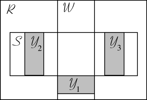
Figure 1. A situation in which the Markov property holds for sets blocking $\mathcal{W}$ but not for general blocking sets. $\mathcal{S}$ is the full horizontal rectangle, and $\mathcal{W}$ is the full vertical rectangle.

Figure 1 depicts a situation for the FK model in which the Markov property holds for sets blocking $\mathcal{W}$, but not for general blocking sets. Let $\mathcal{E}$ be the union of the horizontal rectangle $\mathcal{S}$ and the vertical rectangle $\mathcal{W}$. The boundary condition on $\mathcal{E}$ consists of open bonds on the horseshoe-shaped regions comprising $\mathcal{R}\backslash(\mathcal{S}\cup\mathcal{W})$, and all bonds outside $\mathcal{R}$ closed. The Markov property does not hold for the horizontal blocking set $\mathcal{Y}_{1}$, because the presence or absense of a connection from one component of $\mathcal{R}\backslash(\mathcal{S}\cup\mathcal{W})$ to the other component underneath $\mathcal{Y}_{1}$ affects the probability of a connection between these components above $\mathcal{Y}_{1}$. However, the Markov property does hold for sets blocking $\mathcal{E}$, such as $\mathcal{Y}_{2},\mathcal{Y}_{3}$ or $\mathcal{Y}_{2}\cup\mathcal{Y}_{3}$; in fact $\mathcal{W}$ is blockable in $\mathcal{E}$ under $\mathcal{W}$.

For $\mathcal{R}\subset\mathcal{B}(\mathbb{Z}^{d}),r>0$ and $x\in V(\mathcal{R})$ define the $d_{\mathcal{R}}$-ball

$$B_{\mathcal{R}}(x,r)=\{b=\langle yz\rangle\in\mathcal{R}:d_{\mathcal{R}}(x,y)\leq r,d_{\mathcal{R}}(x,z)\leq r\}.$$

For $c>1,r\geq 1$, a $c$-approximate r-neighborhood of a point $x\in\mathbb{R}^{d}$ in $\mathcal{R}$ is a set $\mathcal{N}$ of bonds satisfying $B_{\mathcal{R}}(x,r/c)\subset\mathcal{N}\subset B_{\mathcal{R}}(x,r)$. A $c$-approximate $r$-neighborhood of a bond $b$ is a $c$-approximate $r$-neighborhood of an endpoint of $b$, say the one closest to the origin. We make analogous definitions for a set $\Lambda$ of sites in place of the set $\mathcal{R}$ of bonds.

A separated-occurrence inequality for finite volumes, in the form (1.6), is most meaningful if the constants $c_{3},\epsilon_{2}$ are uniform over some class of finite volumes and/or boundary conditions; for a single finite-volume measure $P$ with bounded energy, there is always some choice of $c_{3},\epsilon_{2}$ that makes the inequality trivially true. As seen in the related context of [3] for the FK model, properties like exponential decay and mixing may hold in infinite volume but fail to hold (appropriately reformulated) uniformly in finite volumes under certain kinds of boundary conditions. Therefore it is necessary to restrict to special classes of boundary conditions. To give a unified presentation without excessive numbers of cases, we use the following formulation for bond models. $\mathfrak{R}$ is a collection of finite subsets of $\mathcal{B}(\mathbb{Z}^{d})$, and for each $\mathcal{R}\in\mathfrak{R}$ we have a collection $\mathfrak{M}_{\mathcal{R}}$ of probability measures on $\{0,1\}^{\mathcal{R}}$. We seek separated-occurrence inequalities which are uniform over $\mathfrak{M}=\cup_{\mathcal{R}\in\mathfrak{R}}\ \mathfrak{M}_{\mathcal{R}}$, that is, the constants $c_{3},\epsilon_{2}$ (as in (1.6)) do not depend on $P\in\mathfrak{M}$. Typically, each $\mathfrak{M}_{\mathcal{R}}$ might consist of some class of bond or site boundary conditions, on $\mathcal{R}$, for some fixed bond percolation model on $\mathcal{B}(\mathbb{Z}^{d})$. In addition we use auxiliary collections $\mathfrak{V}_{\mathcal{R}}\subset\mathfrak{S}_{\mathcal{R}}$ of subsets of $\mathcal{R}$ and an auxiliary collection $\mathfrak{N}$ not depending on $\mathcal{R}$; we write $\mathfrak{V}=\{\mathfrak{V}_{\mathcal{R}}:\mathcal{R}\in\mathfrak{R}\}$ and $\mathfrak{S}=\{\mathfrak{S}_{\mathcal{R}}:\mathcal{R}\in\mathfrak{R}\}$. For technical convenience we require that $|\mathcal{V}|\geq 2$ for all $\mathcal{V}\in\mathfrak{V}_{\mathcal{R}}$. We will refer to this setup—that is, to a designation of collections $\mathfrak{R},\mathfrak{V},\mathfrak{S},\mathfrak{M},\mathfrak{N}$ as described—as our standard bond percolation setup. As we have mentioned, one of the two events in the separated-occurrence inequality may be restricted to occur on a particular $\mathcal{D}\subset\mathcal{R}$; the sets in $\mathfrak{V}_{\mathcal{R}}$ are neighborhoods of such $\mathcal{D}$ in $\mathcal{R}$, the sets in $\mathfrak{S}_{\mathcal{R}}$ are subsets of such neighborhoods, and the sets in $\mathfrak{N}$ are approximate neighborhoods in sets $\mathcal{S}\in\mathfrak{S}_{\mathcal{R}}$. (One can take $\mathcal{D}=\mathcal{R}$ and hence $\mathfrak{V}_{\mathcal{R}}=\{\mathcal{R}\}$ if desired, but allowing smaller $\mathcal{D}$ means we may reduce the required separation $r$ between the events in question.)

Like the proof in [25] of the van den Berg-Kesten inequality, our proofs of separated-occurrence inequalities involve a process of splitting bonds one at a time. In our context the bonds to be split are those in some neighborhood $\mathcal{V}\in\mathfrak{V}_{\mathcal{R}}$ of $\mathcal{D}$ in $\mathcal{R}$. We may view this procedure as the filling of $\mathcal{V}$ sequentially with split bonds. As this filling process proceeds we require, among other things, that the set $\mathcal{S}\subset\mathcal{V}$ of split bonds always satisfy $\mathcal{S}\in\mathfrak{S}_{\mathcal{R}}$. We will need assumptions not just on the original collections $\mathfrak{R},\mathfrak{M}$ but also on $\mathfrak{V},\mathfrak{S}$ and certain augmented collections of measures derived from $\mathfrak{M}$. We have no general method for specifying the collections $\mathfrak{V},\mathfrak{S}$ given a choice of original collections $\mathfrak{R}$ and $\mathfrak{M}$, but in the specific examples we will consider, it is not particularly difficult to do so, as we will see, though the methods are rather ad hoc.

Definition 1.1.

Let $\mathfrak{R},\mathfrak{V},\mathfrak{S},\mathfrak{M}$ be as above: $\mathfrak{R}$ is a collection of subsets of $\mathcal{B}(\mathbb{Z}^{d})$, and for each $\mathcal{R}\in\mathfrak{R},\ \mathfrak{V}_{\mathcal{R}}\subset\mathfrak{S}_{\mathcal{R}}$ are collections of subsets of $\mathcal{R}$ and $\mathfrak{M}_{\mathcal{R}}$ is a collection of probability measures on $\{0,1\}^{\mathcal{R}}$. A collection $\mathfrak{N}$ of subsets of $\mathcal{B}(\mathbb{Z}^{d})$ is a neighborhood collection for $\mathfrak{S}$ if there exists $c>0$ such that for every $\mathcal{S}\in\mathfrak{R}\cup(\cup_{\mathcal{R}\in\mathfrak{R}}\ \mathfrak{S}_{\mathcal{R}}),x\in V(\mathcal{S})$ and $r>0$, $\mathfrak{N}$ contains a $c$-approximate $r$-neighborhood of $x$ in $\mathcal{S}$. The corresponding augmented collections of measures are

$$\mathfrak{M}_{w}^{+}(\mathfrak{N},\mathfrak{R})=\left\{P(\omega_{\mathcal{N}}\in\cdot\mid\omega_{\mathcal{R}\backslash\mathcal{N}}=\rho_{\mathcal{R}\backslash\mathcal{N}}^{1}):\mathcal{N}\in\mathfrak{N},\mathcal{R}\in\mathfrak{R},\mathcal{N}\subset\mathcal{R},P\in\mathfrak{M}\right\}$$

and

$$\mathfrak{M}^{+}(\mathfrak{S},\mathfrak{R})=\left\{P(\omega_{\mathcal{S}}\in\cdot\mid\omega_{\mathcal{R}\backslash\mathcal{S}}=\rho_{\mathcal{R}\backslash\mathcal{S}}^{i}):\mathcal{R}\in\mathfrak{R},\mathcal{S}\in\mathfrak{S}_{\mathcal{R}},P\in\mathfrak{M},i=0,1\right\}.$$

Let $c>1$ and $r>0$; given $\mathcal{R}\in\mathfrak{R}$, $P\in\mathfrak{M}_{\mathcal{R}}$, $\mathcal{S}\subset\mathcal{R}$ and $e\in\mathcal{R}\backslash\mathcal{S}$ we say that $e$ is neighborhood-appendable to $\mathcal{S}$ for $(c,r,\mathcal{R},P,\mathfrak{N})$ if there exists a $c$-approximate $r$-neighborhood $\mathcal{W}\in\mathfrak{N}$ of $e$ in $\mathcal{R}$ such that either $\mathcal{W}$ or $\mathcal{W}\backslash\mathcal{S}$ is blockable in $\mathcal{S}\cup\mathcal{W}$ under $P$ (see Figure 1.) We say that $\mathcal{V}\subset\mathcal{R}$ is fillable compatibly with $(c,r,\mathcal{R},P,\mathfrak{S}_{\mathcal{R}},\mathfrak{N})$ if there exists an ordering $b_{1},..,b_{n}$ of the bonds of $\mathcal{V}$ such that for all $0\leq k<n$, we have (i) $\mathcal{S}_{k}=\{b_{1},..,b_{k}\}\in\mathfrak{S}_{\mathcal{R}}$, (ii) $b_{k+1}$ is neighborhood-appendable to $\mathcal{S}_{k}$ for $(c,r,\mathcal{R},P,\mathfrak{N})$, and (iii) every $e\in\mathcal{R}\backslash\mathcal{S}$ is neighborhood-appendable to $\mathcal{S}_{k}$ for $(c,r/4,\mathcal{R},P,\mathfrak{N})$. For $R>1$ we say that $(\mathfrak{R},\mathfrak{V},\mathfrak{S},\mathfrak{M},\mathfrak{N})$ is filling-compatible at scale $R$ if for some $c>1$, for every $\mathcal{R}\in\mathfrak{R},\mathcal{V}\in\mathfrak{V}_{\mathcal{R}},P\in\mathfrak{M}_{\mathcal{R}}$ and $1\leq r<R$, $\mathcal{V}$ is fillable compatibly with $(c,r,\mathcal{R},P,\mathfrak{S}_{\mathcal{R}},\mathfrak{N})$. In this context we refer to such $c$ as suitable. We omit the wording “at scale $R$” when $R=\infty$.

Let us consider such properties for some natural classes $\mathfrak{R},\mathfrak{V},\mathfrak{S},\mathfrak{M}$. It is worth pointing out that we would certainly like the class $\mathfrak{R}$ to be as large as possible, but it is less important that the classes $\mathfrak{V}_{\mathcal{R}}$ be large, since the sets $\mathcal{V}\in\mathfrak{V}_{\mathcal{R}}$ are used only to in effect enclose a neighborhood of the set $\mathcal{D}$, where one of the events $A,B$ occurs, in a “nice” set that can serve as the set of split bonds.

For $\mathcal{R}\subset\mathcal{B}(\mathbb{Z}^{d})$ and $k\leq d$ let $\mathcal{R}_{k}$ be the union of all $k$-dimensional unit cubes having all edges in $\mathcal{R}$, and let $\mathcal{R}^{\operatorname{solid}}=\cup_{k\leq d}\mathcal{R}_{k}$. We say that $\mathcal{R}$ is simply lattice-connected, abbreviated SLC, if $\mathcal{R}^{\operatorname{solid}}$ is simply connected. For $d=2$, it is easy to see that $\mathcal{R}$ is SLC if and only if both $\mathcal{R}$ and $(\mathcal{R}^{c})^{*}$ are connected sets of bonds and dual bonds respectively, which was the definition used in [3]. For $\Lambda\subset\mathbb{Z}^{d}$ we say $\Lambda$ is simply lattice-connected if $\mathcal{B}(\Lambda)$ is simply lattice-connected. For $d=2$ simple lattice-connectedness is a natural assumption in the context of uniform exponential decay and strong mixing, in view of [3]. The SLC property also fits well with our need to form enlarged collections, as Example 1.2 below shows. For $\Gamma$ a self-avoiding lattice circuit let $\operatorname{Int}(\Gamma)$ denote the set of all bonds strictly inside $\Gamma$ (excluding endpoints). For $d=2$, we say that $\mathcal{R}$ is circuit-bounded if there exists a self-avoiding lattice circuit, denoted $\Gamma_{\mathcal{R}}$, such that $\mathcal{R}=\Gamma_{\mathcal{R}}\cup\operatorname{Int}(\Gamma_{\mathcal{R}})$. For $\mathcal{R}$ circuit-bounded and $\mathcal{B}\subset\operatorname{Int}(\mathcal{R})$, the boundary closure of $\mathcal{B}$ in $\mathcal{R}$ is $\mathcal{B}\cup\{\langle xy\rangle\in\Gamma_{\mathcal{R}}:x,y\in V(\mathcal{B})\}$. We say that $\mathcal{R}$ is lattice-convex if it has the form $\{b\in\mathcal{B}(\mathbb{Z}^{d}):b\subset C\}$ for some convex $C$. If $C$ is a rectangle (which we may assume has vertices in $\mathbb{Z}^{d}$) then we call $\mathcal{R}$ a lattice rectangle, and we let $\Gamma_{\mathcal{R}}$ denote the outer surface $\{b\in\mathcal{R}:b\subset\partial C\}$ and let $\operatorname{Int}(\mathcal{R})=\mathcal{R}\backslash\Gamma_{\mathcal{R}}$. If $\mathcal{R}$ is a lattice rectangle (or a circuit-bounded set, or a $d_{\mathcal{A}}$-ball for some $\mathcal{A}$), $\mathcal{B}\subset\mathcal{R}$ and every bond of $\mathcal{R}\backslash\mathcal{B}$ abuts $\mathcal{R}^{c}$, then we call $\mathcal{B}$ an approximate lattice rectangle (or approximate circuit-bounded set, or approximate $d_{\mathcal{A}}$-ball.) and we refer to $\mathcal{R}$ as the completed lattice rectangle (or circuit-bounded set, or $d_{\mathcal{A}}$-ball.) A lattice rectangle or a circuit-bounded set of bonds $\mathcal{R}$ is minimally fat if $\operatorname{Int}(\Gamma_{\mathcal{R}})$ is connected. An approximate lattice rectangle $\mathcal{R}$, with completed lattice rectangle $\tilde{\mathcal{R}}$, is regular if for every bond $e\in\mathcal{R}\cap\Gamma_{\tilde{\mathcal{R}}}$, all bonds in $\operatorname{Int}(\tilde{\mathcal{R}})$ which abut $e$ (note there are at most two) are in $\mathcal{R}$.

Example 1.2.

Let $\mathfrak{R}$ be the class of all minimally fat lattice rectangles in $\mathcal{B}(\mathbb{Z}^{d})$, let $\mathfrak{S}_{\mathcal{R}}$ be the class of all approximate lattice rectangles $\mathcal{S}\subset\mathcal{R}$ with $\mathcal{R}\backslash\mathcal{S}$ connected, and let $\mathfrak{V}_{\mathcal{R}}$ be the class of all lattice rectangles $\mathcal{V}\subset\mathcal{R}$ such that $\mathcal{R}\backslash\mathcal{V}$ is connected and $|\mathcal{V}|\geq 2$. (Note that for $d=2$ this excludes those $\mathcal{V}$ which intersect $\Gamma_{\mathcal{R}}$ only in two opposite faces.) Let $\mathfrak{N}$ be the class of all approximate lattice rectangles in $\mathcal{B}(\mathbb{Z}^{d})$. Let $P$ be an FK model on $\mathcal{B}(\mathbb{Z}^{2})$ (see Section 2 for a description), and let $\mathfrak{M}$ be the class of all the associated finite-volume FK measures $P_{\mathcal{R},*}$ with $\mathcal{R}\in\mathfrak{R}$ and with $*=w$ or $f$. Assume that either $i=1$ or there are no external fields. In view of Lemma 2.1 below, given $\mathcal{R}\in\mathfrak{R},\mathcal{V}\in\mathfrak{V}_{\mathcal{R}}$ and $r\geq 1$, we want to fill $\mathcal{V}$ in such a way that for all $k$, for $\mathcal{S}_{k}$ as in Definition 1.1 and $e\in\mathcal{R}\backslash\mathcal{S}_{k}$, for some $d$-approximate $r$-neighborhood $\mathcal{W}$ of $e$ in $\mathcal{R}$, we have the following: (a) $\mathcal{S}_{k}$ is an approximate lattice rectangle, (b) $\mathcal{R}\backslash\mathcal{S}_{k}$ is connected, and (c) each component of $\mathcal{S}_{k}\backslash\mathcal{W}$ is an approximate latttice rectangle which abuts at most one component of $\mathcal{R}\backslash(\mathcal{S}_{k}\cup\mathcal{W})$. We can always choose $\mathcal{W}$ to be a lattice rectangle which either does not intersect $\mathcal{S}_{k}$ or intersects the interior of the completed $\mathcal{S}_{k}$; this means that within (c) there are two cases: (c^′) $\mathcal{R}\backslash(\mathcal{S}_{k}\cup\mathcal{W})$ is connected and (c^′′) $\mathcal{R}\backslash(\mathcal{S}_{k}\cup\mathcal{W})$ has two components ($\mathcal{W}$ “slices through” $\mathcal{R}$.) It follows from Lemma 2.1 that under (c^′), $\mathcal{W}\backslash\mathcal{S}_{k}$ is blockable in $\mathcal{S}_{k}\cup\mathcal{W}$ under $P_{\mathcal{R},*}$, while under (c^′′), $\mathcal{W}$ is blockable in $\mathcal{S}_{k}\cup\mathcal{W}$ under $P_{\mathcal{R},*}$. (Here $*=w$ or $f$.) It will follow that $(\mathfrak{R},\mathfrak{V},\mathfrak{S},\mathfrak{M},\mathfrak{N})$ is filling-compatible.

In fact, to obtain (a), (b), (c), we can fill $\mathcal{V}$ by first filling $\mathcal{V}\cap\operatorname{Int}(\mathcal{R})$ and then filling $\mathcal{V}\cap\Gamma_{\mathcal{R}}$. It is not hard to see that during the filling of $\mathcal{V}\cap\operatorname{Int}(\mathcal{R})$ we can keep $\mathcal{S}_{k}$ an SLC regular approximate lattice rectangle so that all of $\mathcal{R}\backslash\mathcal{S}_{k}$ is connected to $\Gamma_{\mathcal{R}}$, which ensures that $\mathcal{R}\backslash\mathcal{S}_{k}$ is connected. Since $\mathcal{W}$ is a lattice rectangle, $\mathcal{R}\backslash\mathcal{W}$ has at most 2 components $\mathcal{C}_{i}$, and $\mathcal{C}_{i}\cap\Gamma_{\mathcal{R}}$ is nonempty and connected for each $i$. If there are 2 components $\mathcal{C}_{i}$, then, since $\mathcal{S}_{k}$ is regular, each $\mathcal{S}_{k}\cap\mathcal{C}_{i}$ is an approximate lattice rectangle and (c^′′) holds. If there is only one component $\mathcal{C}_{1}=\mathcal{R}\backslash\mathcal{W}$, then, since $\mathcal{S}_{k}\subset\operatorname{Int}(\mathcal{R})$, we have $\mathcal{R}\backslash(\mathcal{S}_{k}\cup\mathcal{W})$ connected, i.e. (c^′) holds. (Note that for $d\geq 3$, when there is only one component $\mathcal{C}_{1}$, we could have $\mathcal{S}_{k}\backslash\mathcal{W}$ connected but not SLC, meaning (c) fails.) Thus all of our conditions (a), (b) and (c) remain satisfied during the filling of $\mathcal{V}\cap\operatorname{Int}(\mathcal{R})$. If $\mathcal{V}\cap\Gamma_{\mathcal{R}}$ is empty we are done; if $\mathcal{V}\cap\Gamma_{\mathcal{R}}$ is nonempty then by assumption we have $\mathcal{R}\backslash\mathcal{V}$ connected. But then it is not hard to see that we can fill the rest of $\mathcal{V}$ (i.e. fill $\mathcal{V}\cap\Gamma_{\mathcal{R}}$) keeping $\Gamma_{\mathcal{R}}\cap\mathcal{S}_{k}$ and $\Gamma_{\mathcal{R}}\backslash\mathcal{S}_{k}$ both connected, with $\mathcal{S}_{k}$ having an approximately rectangular intersection with each face of $\mathcal{R}$. Following this procedure we see that our preceding verification of (a), (b) and (c) remains valid as we fill $\mathcal{V}\cap\Gamma_{\mathcal{R}}$.

It is “straightforward but tedious” to extend Example 1.2 to allow general lattice-convex sets in $\mathfrak{R}$ and $\mathfrak{V}_{\mathcal{R}}$, instead of just rectangles. In two dimensions we can be much more general, as the next example shows.

Example 1.3.

Let $\mathfrak{R}$ be class of all circuit-bounded subsets of $\mathcal{B}(\mathbb{Z}^{2})$. For $\mathcal{R}\in\mathfrak{R}$ let

$$\mathfrak{V}_{\mathcal{R}}=\{\mathcal{V}\subset\mathcal{R}:\mathcal{V}$$ is the boundary closure of

$$\text{some }d_{\operatorname{Int}(\mathcal{R})}-\text{ball in }\mathcal{R},\mathcal{R}\backslash\mathcal{V}\text{ is connected, and }|\mathcal{V}|\geq 2\},$$

and let $\mathfrak{S}_{\mathcal{R}}$ be the class of all SLC $\mathcal{S}\subset\mathcal{R}$ with $\mathcal{R}\backslash\mathcal{S}$ connected. Let $\mathfrak{M}$ be the class of all the associated finite-volume FK measures $P_{\mathcal{R},*}$ with $\mathcal{R}\in\mathfrak{R}$ and with $*=w$ or $f$, and let $\mathfrak{N}$ be the class of all finite SLC subsets of $\mathcal{B}(\mathbb{Z}^{2})$. Similarly to Example 1.2, given $\mathcal{R}\in\mathfrak{R}$ and $\mathcal{V}=\{b_{1},..,b_{n}\}\in\mathfrak{V}_{\mathcal{R}}$ we want to fill $\mathcal{V}$ so that (a) $\mathcal{S}_{k}=\{b_{1},..,b_{k}\}$ is SLC, (b) $\mathcal{R}\backslash\mathcal{S}_{k}$ is connected, and (c) for $e\in\mathcal{R}\backslash\mathcal{S}_{k}$, for some $d_{\mathcal{R}}$-ball $\mathcal{W}$ centered at an endpoint of $e$, each component of $\mathcal{S}_{k}\backslash\mathcal{W}$ abuts at most one component of $\mathcal{R}\backslash(\mathcal{S}_{k}\cup\mathcal{W})$.

A useful observation about $d_{\mathcal{R}}$-balls in the plane (also valid for $d_{\operatorname{Int}(\mathcal{R})}$-balls) is as follows. The “outer surface inside $\Gamma_{\mathcal{R}}$” for a ball $B_{\mathcal{R}}(z,k)$, by which we mean $\{w\in V(\mathcal{R})\backslash V(\Gamma_{\mathcal{R}}):d_{\mathcal{R}}(z,w)=k\}$, must fall along diagonal lines, i.e. it cannot contain two adjacent sites, as is easily seen.

We first fill $\mathcal{V}\cap\operatorname{Int}(\mathcal{R})$. We order the bonds of $\mathcal{V}\cap\operatorname{Int}(\mathcal{R})=\{b_{1},..,b_{m}\}$ in order of increasing $d_{\operatorname{Int}(\mathcal{R})}$-distance from $x$, breaking ties in such a way that $\mathcal{S}_{k}=\{b_{1},..,b_{k}\}$ remains SLC. This means that each $\mathcal{S}_{k}$ is an approximate $d_{\operatorname{Int}(\mathcal{R})}$-ball. Now (a) is clear, and (b) follows from the fact that $\Gamma_{\mathcal{R}}\subset\mathcal{R}\backslash\mathcal{S}_{k}$. For (c), let $\mathcal{W}=B_{\mathcal{R}}(y,l)$ for an endpoint $y$ of $e$ and some $l>1$, and suppose $\mathcal{S}_{k}$ is an approximate $d_{\operatorname{Int}(\mathcal{R})}$-ball, for which the completed $d_{\operatorname{Int}(\mathcal{R})}$-ball is $B_{\operatorname{Int}(\mathcal{R})}(x,m)$ for some $m>1$. If $\mathcal{W}\cap\mathcal{S}_{k}=\phi$ then after shrinking $\mathcal{W}$ slightly (say, decrease $l$ by 2), $\mathcal{R}\backslash(\mathcal{S}_{k}\cup\mathcal{W})$ becomes connected, and then (c) is trivial. Hence we assume $\mathcal{W}\cap\mathcal{S}_{k}\neq\phi$. If we enlarge $\mathcal{W}$ slightly (say, increase $l$ by 2), this ensures that $\mathcal{S}_{k}\cup\mathcal{W}$ is connected, which means that each component of $\mathcal{R}\backslash(\mathcal{S}_{k}\cup\mathcal{W})$ contains at most one segment of $\Gamma_{\mathcal{R}}$. We claim that every component of $\mathcal{R}\backslash(\mathcal{S}_{k}\cup\mathcal{W})$ contains exactly one segment of $\gamma$. Suppose instead that some component $\mathcal{A}$ of $\mathcal{R}\backslash(\mathcal{S}_{k}\cup\mathcal{W})$ does not intersect $\Gamma_{\mathcal{R}}$; since $\mathcal{S}_{k}$ and $\mathcal{W}$ are SLC, loosely speaking we conclude that $\mathcal{S}_{k}$ and $\mathcal{W}$ must intersect on two sides of $\mathcal{A}$ in such a way that their union surrounds $\mathcal{A}$. More precisely, there must exist sites $u,v\in V(\mathcal{S}_{k})\cap V(\mathcal{W})$ and lattice paths $\gamma_{x\leftrightarrow u},\gamma_{x\leftrightarrow v},\gamma_{y\leftrightarrow u},\gamma_{y\leftrightarrow v}$ of minimal length (at most $m,m,l,l$ respectively), with the union of these paths containing a circuit surrounding $\mathcal{A}$. Here $\gamma_{g\leftrightarrow h}$ denotes a path from $g$ to $h$. (Note that for general SLC $\mathcal{W}$ and $\mathcal{S}_{k}$, $\mathcal{R}\backslash(\mathcal{S}_{k}\cup\mathcal{W})$ could include one or more components consisting of a single bond with one endpoint in $V(\mathcal{W})$ and the other in $V(\mathcal{S}_{k})$, not surrounded by such lattice paths, but that is not possible for in the present situation, due to our observation about the outer surface inside $\Gamma_{\mathcal{R}}$ for a ball.) For lattice paths $\gamma,\tilde{\gamma}$ in $\mathcal{R}$ having the same endpoints, we say that $\tilde{\gamma}$ is directly obtainable from $\gamma$ by contraction if we can change $\gamma$ to $\tilde{\gamma}$ by one of the following two procedures: (1) select a lattice square $Q$ such that two sides of $Q$ are consecutive bonds of $\gamma$, and replace these two bonds with the other two sides of $Q$ (equivalently, replace the common site of the two bonds with the opposite corner of $Q$, if we view the path as a sequence of sites), or (2) select a lattice square $Q$ such that three sides of $Q$ are consecutive bonds of $\gamma$, and replace them with the other side of $Q$ (i.e., shortcut the trip around $Q$.) Again for paths $\gamma$ and $\tilde{\gamma}$ having the same endpoints $g,h$, we say that $\tilde{\gamma}$ is obtainable from $\gamma$ by contraction in $\mathcal{R}$ if there is a sequence of lattice paths in $\mathcal{R}$, each from $g$ to $h$, starting with $\gamma$ and ending with $\tilde{\gamma}$, each directly obtainable from the previous one by contraction. We may assume the paths $\gamma_{x\leftrightarrow u},\gamma_{x\leftrightarrow v},\gamma_{y\leftrightarrow u},\gamma_{y\leftrightarrow v}$ are disjoint; if not, we replace the starting site $x$ with the last common site of $\gamma_{x\leftrightarrow u}$ and $\gamma_{x\leftrightarrow v}$ on the way to $u$ and $v$, respectively, from $x$, and similarly for $y$. Consider the two paths $\alpha_{0}=\gamma_{x\leftrightarrow u}\cup\gamma_{y\leftrightarrow u}$ and $\tilde{\alpha}_{0}=\gamma_{x\leftrightarrow v}\cup\gamma_{y\leftrightarrow v}$, each from $x$ to $y$. It is easy to see that there is a path $\alpha$ between these two paths which is obtainable from both paths by contraction in $\mathcal{R}$. The various paths, call them $\alpha_{i}$ and $\tilde{\alpha}_{i}$, obtained along the way from $\alpha_{0}$ and $\tilde{\alpha}_{0}$ to $\alpha$ are each no longer than the original paths $\alpha_{0}$ and $\tilde{\alpha}_{0}$, and every bond between $\alpha_{0}$ and $\tilde{\alpha}_{0}$ is on one of the paths $\alpha_{i}$ or $\tilde{\alpha_{i}}$. The contraction aspect means that $\alpha_{i},\tilde{\alpha_{i}}\subset B_{\mathcal{R}}(x,m)\cup\mathcal{W}$, so we conclude that $\mathcal{A}\subset B_{\mathcal{R}}(x,m)\cup\mathcal{W}$, in contradiction to the definition of $\mathcal{A}$. This establishes our claim that each nontrivial component of $\mathcal{R}\backslash(\mathcal{S}_{k}\cup\mathcal{W})$, and therefore also each component of $\mathcal{R}\backslash(\mathcal{S}_{k}\cup\mathcal{W})$, contains exactly one segment of $\Gamma_{\mathcal{R}}$. We thus have the following picture: $\mathcal{R}$ and $\mathcal{W}$ are SLC, so each component $\mathcal{C}$ of $\mathcal{R}\backslash\mathcal{W}$ includes exactly one segment, call it $\gamma_{\mathcal{C}}$, of $\Gamma_{\mathcal{R}}$. When we remove the set $\mathcal{S}_{k}$ to obtain $\mathcal{R}\backslash(\mathcal{S}_{k}\cup\mathcal{W})$, the remaining portion $\mathcal{C}\backslash\mathcal{S}_{k}$ of $\mathcal{C}$ is all connected to $\gamma_{\mathcal{C}}$ and is the only component of $\mathcal{R}\backslash(\mathcal{S}_{k}\cup\mathcal{W})$ which abuts $\mathcal{S}_{k}\cap\mathcal{C}$. This proves (c), and we have (a), (b), (c) while filling $\operatorname{Int}(\Gamma_{\mathcal{R}})$.

Since $\mathcal{V}$ and $\mathcal{R}\backslash\mathcal{V}$ are connected, $\mathcal{V}\cap\Gamma_{\mathcal{R}}$ is a single segment, so after $\mathcal{V}\cap\operatorname{Int}(\mathcal{R})$ is filled, we can fill $\mathcal{V}\cap\Gamma_{\mathcal{R}}$ by starting at one end of this segment and proceeding to the other end. This keeps the part of $\Gamma_{\mathcal{R}}$ outside $\mathcal{S}_{k}$ connected, and the above proof of (a), (b), (c) remains valid (though now, in (c^′′), there may be more than two components.) As in Example 1.2, this shows that $(\mathfrak{R},\mathfrak{V},\mathfrak{S},\mathfrak{M},\mathfrak{N})$ is filling-compatible.

As Examples 1.2 and 1.3 show, it is sometimes necessary to augment a natural collection, like the rectangles or the circuit-bounded sets, to obtain classes $\mathfrak{S},\mathfrak{V},\mathfrak{N}$ having filling-compatibility, but this seems to be only a minor technical obstactle to the applicability of our results to natural cases.

When dealing with the Ising model we will not have to restrict boundary conditions, so in place of Definition 1.1 we can use the following simpler ideas. We say that a collection $\mathfrak{L}$ of finite subsets of $\mathbb{Z}^{d}$ has the approximate neighborhood property if for some $c>1$, for every $\Lambda\in\mathfrak{L}$ and $x\in\Lambda$, $\mathfrak{L}$ includes a $c$-approximate $r$-neighborhood of $x$ in $\Lambda$ (A similar property termed inheriting was used in [3]; the two are interchangeable for our purposes.) We say that $\mathfrak{L}$ is fillable if for every $\Lambda\in\mathfrak{L}$ there exists and ordering $x_{1},..,x_{n}$ of $\Lambda$ such that for all $1\leq k\leq n,\{x_{1},..,x_{k}\}\in\mathfrak{L}$. Note that, in contrast to the analogous properties (Definition 1.1) for bond models, here we need not incorporate collections of measures into the definitions, because our collection of measures will always consist of all Ising models on all $\Lambda\in\mathfrak{L}$ with arbitrary boundary conditions.

We turn now to some definitions related to further conditions we will impose on the collection $\mathfrak{M}$ of measures. For ordered $J$, a probability measure $P$ on $J^{\Delta}$ for some finite $\Delta$ is said to have the FKG property if $A,B$ increasing implies $P(A\cap B)\geq P(A)P(B)$. $P$ is said to satisfy the FKG lattice condition if

(1.8) $$P(\omega\vee\omega^{\prime})P(\omega\wedge\omega^{\prime})\geq P(\omega)P(\omega^{\prime})\quad\text{for all }\omega,\omega^{\prime},$$

where $\vee$ and $\wedge$ denote the coordinatewise maximum and minimum, respectively. This implies that $P(\omega_{\Lambda}\in\cdot\mid\omega_{\Delta\backslash\Lambda}=\eta_{\Delta\backslash\Lambda})$ has the FKG property for all $\Lambda$ and $\eta$ [19]. In a mild abuse of notation, for a bond $e$ we write $\omega\vee e$ for the configuration taking value 1 at $e$ and agreeing with $\omega$ at all other bonds. Then (1.8) is equivalent to

$$\frac{P(\omega\vee e)}{P(\omega)}\text{ is an increasing function of }\omega\text{ for each fixed }e.$$

For $Q$ another probability measure, we say that $P$ FKG-dominates $Q$ if for every nondecreasing function $f$ on $J^{\Delta}$,

$$\int fdP\geq\int fdQ.$$

We say that the collection $\mathfrak{M}=\cup_{\mathcal{R}\in\mathfrak{R}}\ \mathfrak{M}_{\mathcal{R}}$ has uniform exponential decay of connectivity if there exist $C,\lambda>0$ such that for every $\mathcal{R}\in\mathfrak{R}$ and $P\in\mathfrak{M}_{\mathcal{R}}$,

$$P(x\leftrightarrow y\text{ via a path in }\mathcal{R})\leq Ce^{-\lambda d_{\mathcal{R}}(x,y)}\quad\text{for all }x,y\in V(\mathcal{R}).$$

The finite-volume analog of ratio weak mixing can be formulated for a collection $\mathfrak{M}=\cup_{\mathcal{R}\in\mathfrak{R}}\ \mathfrak{M}_{\mathcal{R}}$ of measures, as follows. We say that $\mathfrak{M}$ has the ratio strong mixing property if there exist $C,\lambda>0$ such that for all $\mathcal{R}\in\mathfrak{R},P\in\mathfrak{M}_{\mathcal{R}}$ and $\mathcal{E},\mathcal{F}\subset\mathcal{R}$,

(1.9) $$\sup \left\{\left|\frac{P(A\cap B)}{P(A)P(B)}-1\right|:A\in\mathcal{G}_{\mathcal{E}},B\in\mathcal{G}_{\mathcal{F}},P(A)P(B)>0\right\}$$

$$\leq C\sum_{x\in V(\mathcal{E}),y\in V(\mathcal{F})}e^{-\lambda d_{\mathcal{R}}(x,y)},$$

whenever the right side of (1.9) is less than 1. This definition was given in [3] for the special case of a fixed bond percolation model with some class of site or bond boundary conditions.

A coupling of two probability measures $P_{1}$ and $P_{2}$ on some set $J^{\Delta}$ is a probability measure $\mathbb{P}$ on $J^{\Delta}\times J^{\Delta}$ with marginals $P_{1}$ and $P_{2}$ (in order).

For $\Delta\subset\Lambda\subset\mathbb{Z}^{d}$ and $r>0$ let

$$\Delta^{r}(\Lambda)=\{x\in\Lambda:d_{\mathcal{B}(\Lambda)}(x,\Delta)\leq r\},\qquad\Delta^{r}=\Delta^{r}(\mathbb{Z}^{d}).$$

Similarly for $\mathcal{D}\subset\mathcal{R}\subset\mathcal{B}(\mathbb{Z}^{d})$ let

$$\mathcal{D}^{r}(\mathcal{R})=\{b\in\mathcal{R}:d_{\mathcal{R}}(b,\mathcal{D})\leq r\},\qquad\mathcal{D}^{r}=\mathcal{D}^{r}(\mathcal{B}(\mathbb{Z}^{d})).$$

2. Specific Models

The FK model ([12], [13], [14]; see also [2], [15]) is a graphical representation of the Potts model. For a configuration $\omega$ on $\mathcal{R}\subset\mathcal{B}(\mathbb{Z}^{d})$, let $K(\omega)$ denote the number of open clusters in $\omega$ which do not abut $\mathcal{R}^{c}$. For $p\in[0,1]$ and $q>0$, the FK model $P_{\mathcal{R},w}^{p,q}$ (without external fields) on $\mathcal{R}$ with parameters $(p,q)$ and wired boundary condition is defined by the weights

(2.1) $$W(\omega)=p^{|\omega|}(1-p)^{|\mathcal{R}|-|\omega|}q^{K(\omega)}.$$

Here $|\omega|$ means the number of open bonds in $\omega$. Let $K(\omega\mid\rho)$ be the number of open clusters of $(\omega\rho)$ which abut or intersect $\mathcal{R}$. The FK model $P_{\mathcal{R},\rho}^{p,q}$ with bond boundary condition $\rho$ is given by the weights in (2.1) with $K(\omega)$ replaced by $K(\omega\mid\rho)$. When $\rho=\rho^{0}$ or $\rho^{1}$ we replace $\rho$ with $f$ or $w$ in our notation. The infinite-volume measures

$$P^{p,q}=\lim_{\Lambda\nearrow\mathbb{Z}^{d}}P^{p,q}_{\Lambda,*}$$

on $\{0,1\}^{\mathcal{B}(\mathbb{Z}^{d})}$ exist for $*=w$ or $f$ and are translation-invariant. For $p$ below the percolation critical point $p_{c}(q,d)$ we have $P^{p,q}_{w}=P^{p,q}_{f}$ so we omit the subscript. For a summary of basic properties of the FK model, see [15]. In particular, for $q\geq 1$ the FK model satisfies the FKG lattice condition, and we consider only these values of $q$.

We also need to consider site boundary conditions, when we use the FK model as a graphical representation of the Ising model. Given $\Lambda\subset\mathbb{Z}^{d}$ and $\eta\in\{-1,1\}^{\partial\Lambda}$ define

$$\partial\Lambda=\{x\in\Lambda^{c}:x\text{ adjacent to }y\text{ for some }y\in\Lambda\},$$

$$U(\Lambda,\eta)=\bigl{\{}\omega\in\{0,1\}^{\overline{\mathcal{B}}(\Lambda)}:\eta_{x}=\eta_{y}\text{ for every }x,y\in\partial\Lambda\text{ for which }x\leftrightarrow y\text{ in }\omega\bigr{\}}.$$

The FK model $P^{p,q}_{\overline{\mathcal{B}}(\Lambda),\eta}$ with site boundary condition $\eta$ is given by the weights in (2.1), multiplied by $\delta_{U(\Lambda,\eta)}(\omega)$.

For the FK model with external fields $h_{i}$, $i=1,\ldots,q$ and free boundary, the factor $q^{K(\omega)}$ in the weight $W(\omega)$ is replaced by

(2.2) $$\prod_{C\in\mathcal{K}(\omega)}\left((1-p)^{h_{1}s(C)}+(1-p)^{h_{2}s(C)}+\ldots+(1-p)^{h_{q}s(C)}\right),$$

where $\mathcal{K}(\omega)$ is the set of open clusters in $\mathcal{R}$ in the configuration $\omega$ and $s(C)$ denotes the number of sites in the cluster $C$. The parameters are then $(p,q,\{h_{i}\})$; $q$ must be an integer, and we may omit $\{h_{i}\}$ when all external fields are 0. The percolation critical point is denoted $p_{c}(q,d,\{h_{i}\})$. We need only consider $0=h_{1}\geq h_{2}\geq\ldots\geq h_{q}$, so we henceforth assume this in our notation. Species $i$ is called stable if $h_{i}$ is maximal, i.e. $h_{i}=h_{1}=0$. For bond boundary conditions $\rho$ we replace (2.2) with

(2.3) $$\prod_{C\in\mathcal{K}(\omega\mid\rho)}\left((1-p)^{h_{1}s(C)}+(1-p)^{h_{2}s(C)}+\ldots+(1-p)^{h_{q}s(C)}\right),$$

where $\mathcal{K}(\omega\mid\rho)$ is the set of finite open clusters of $(\omega\rho)$ which intersect $V(\mathcal{B})$. For general site boundary conditions $\eta$ for the model on $\overline{\mathcal{B}}(\Lambda)$ the factor (2.2) is multiplied by

(2.4) $$\prod_{C\in\mathcal{K}_{int}(\omega)} \left((1-p)^{h_{1}s(C)}+(1-p)^{h_{2}s(C)}+\ldots+(1-p)^{h_{q}s(C)}\right)$$

$$\times\quad\prod_{C\in\mathcal{K}_{\partial}(\omega)}(1-p)^{h_{i(C)}s(C)}\quad\times\quad\delta_{U(\Lambda,\eta)}(\omega),$$

where $\mathcal{K}_{\partial}(\omega)$ (respectively $\mathcal{K}_{int}(\omega)$) is the set of clusters in the configuration $\omega$ which do (respectively don’t) intersect $\partial\Lambda$ and $i(C)$ is the species for which $\eta_{x}=i$ for all $i\in\partial\Lambda\cap C$. (The existence of such an $i$ is forced by the event $U(\Lambda,\eta)$.)

If $\overline{\mathcal{B}}(\Lambda)^{c}$ is connected then for stable $i$ the wired boundary condition is equivalent to the all-$i$ site boundary condition. For $q\geq 1$, the FK model with external fields satisfies the FKG lattice condition, under any bond boundary condition. We say that $\rho\in\{0,1\}^{\mathcal{R}^{c}}$ is a unique-cluster bond boundary condition if all open bonds in $\rho$ are part of one cluster. We have seen (Figure 1) that in the absense of external fields, an FK model $P_{\mathcal{R},\rho}^{p,q}$ need not in general have the Markov property for blocking sets, but we have the following sufficient conditions.

Lemma 2.1.

Let $\mathcal{R}\subset\mathcal{B}(\mathbb{Z}^{d})$ and consider an FK measure $P_{\mathcal{R},\rho}^{p,q,\{h_{i}\}}$.

(i) Suppose $\rho$ is a unique-cluster bond boundary condition, and suppose that either (a) there are no external fields, (b) there is a unique nonsingleton cluster in $\rho$ and this cluster is infinite, or (c) $\rho=\rho^{0}$. Then $P_{\mathcal{R},\rho}^{p,q,\{h_{i}\}}$ has the Markov property for blocking sets.

(ii) If $\rho$ is arbitrary, there are no external fields, $\mathcal{E}\subset\mathcal{R}$ and each component of $\mathcal{R}\backslash\mathcal{E}$ abuts at most one nonsingleton cluster of $\rho$, then $P_{\mathcal{R},\rho}^{p,q,\{h_{i}\}}$ has the Markov property for sets blocking $\mathcal{E}$.

Proof.

We first prove (i). The FK weight can be written as a product over clusters,

$$\prod_{C\in\mathcal{K}(\omega\mid\rho)}\left(\frac{p}{1-p}\right)^{b(C)}\left((1-p)^{h_{1}s(C)}+(1-p)^{h_{2}s(C)}+\ldots+(1-p)^{h_{q}s(C)}\right),$$

where $s(C)$ and $b(C)$ are the number of sites and bonds, respectively, in the cluster $C$. Let $C_{u}$ denote the unique nonsingleton cluster in $\rho$, when this exists. Let $(\mathcal{X},\mathcal{Y},\mathcal{Z})$ be a blocking partitiion of $\mathcal{R}$, and suppose $\omega=0$ on $\mathcal{Y}$. Note that a group of clusters $C_{1},..,C_{n}$ of $\omega$ may be part of the same cluster, say $\hat{C}$, in $(\omega\rho)$, if $C_{1},..,C_{n}$ are connected together by $C_{u}$; in particular this can occur with some of the $C_{i}$’s on each side of the blocking set $\mathcal{Y}$. However, under (a), (b) or (c), the weight of $\hat{C}$ factors into a product of a weight for each $C_{i}$, and thus the clusters on each side of the blocking set occur independently, yielding the Markov property. The proof of (ii) is similar. ∎

Lemma 2.1 is part of what requires us to use augmented collections instead of using a single $\mathfrak{R}$ and $\mathfrak{M}$ throughout; in Example 1.2, for example, we restrict $\mathfrak{M}$ to free and wired boundary conditions to guarantee the Markov property for blocking sets, but such a restriction would be unnecessary and technically awkward for $\mathfrak{M}_{w}^{+}(\mathfrak{N},\mathfrak{R})$, which does not need the Markov property in our proofs.

The following facts about the FK model are known for $d=2$. For $q=1,q=2,$ and $q\geq 25.72$, we have $p_{c}(q,2)=\tfrac{\sqrt{q}}{1+\sqrt{q}}$ [20], and the connectivity decays exponentially for all $p<p_{c}(q,2)$ [17]. This is believed to be true for all $q$; for $2<q<25.72$ the connectivity is known to decay exponentially at least for all $p<\tfrac{\sqrt{q-1}}{1+\sqrt{q-1}}$, and analogous results hold for other planar lattices [5]. For general $q\geq 1$, if the connectivity decays exponentially then the model has the ratio weak mixing property [7]. (This result is actually given assuming a nonnegative external field applied to at most one species, but the proof carries over without change to arbitrary external fields; the necessary FKG property is proved in [9].)

As shown in [11], for $\beta$ given by $p=1-e^{-\beta}$, a configuration of the Ising model on $\Lambda$ with boundary condition $\eta$ at inverse temperature $\beta$ can be obtained from a configuration $\omega$ of the FK model at $(p,2)$ with site boundary condition $\eta$, by choosing a label for each cluster of $\omega$ independently and uniformly from $\{-1,1\}$; this cluster-labeling construction yields a joint site-bond configuration for which the sites are an Ising model and the bonds are an FK model. When the parameters are related in this way, we call the Ising and FK models corresponding. Alternatively, if one selects an Ising configuration $\sigma_{\Lambda}$ and does independent percolation at density $p$ on the set of bonds

$$\{\langle xy\rangle\in\overline{\mathcal{B}}(\Lambda):(\sigma\eta)_{x}=(\sigma\eta)_{y}\},$$

the resulting bond configuration is a realization of the corresponding FK model. We call this the percolation construction of the FK model.

For the Ising model at inverse temperature $\beta<\beta_{c}(d)$, for $p=1-e^{-\beta}$ and for the FK model without external fields at $(p,2)$, the covariance in the Ising model and the connectivity in the FK model are related by

(2.5) $$\operatorname{cov}(\sigma_{0},\sigma_{x})=P(0\leftrightarrow x);$$

see [2] or [15]. Thus exponential decay of connectivities in the FK model is equivalent to exponential decay of correlations in the corresponding Ising model. Further, $\beta_{c}(d)$ and the percolation critical point $p_{c}(2,d)$ of the FK model are related by

$$p_{c}(2,d)=1-e^{-\beta_{c}(d)};$$

again see [2] or [15]. For $h\neq 0$ we make this a definition, that is, $\beta_{c}(d,h)$ is defined by

$$p_{c}(2,d,h)=1-e^{-\beta_{c}(d,h)},$$

where $p_{c}(2,d,h)$ is the percolation threshhold of the corresponding FK model. (The notation is not meant to imply that $\beta_{c}(d,h)$ is a true critical point.)

3. Statements of Main Theorems

All proofs appear in Section 4. Our first theorem covers bond percolation models in finite volumes $\mathcal{R}$. Note that as discussed in the introduction, one of the two events $A,B$ is restricted to occur somewhere on a fixed set $\mathcal{D}\subset\mathcal{R}$, and the required separation $r$ depends on the size of $\mathcal{D}$. The location of the other event is unrestricted and in particular this location may also be a part of $\mathcal{D}$.

Theorem 3.1.

Let $\mathfrak{R},\mathfrak{V},\mathfrak{S},\mathfrak{M}$ be as in the standard bond percolation setup and let $\mathfrak{N}$ be a neighborhood collection for $\mathfrak{S}$. Suppose that $(\mathfrak{R},\mathfrak{V},\mathfrak{S},\mathfrak{M},\mathfrak{N})$ is filling-compatible, each measure in $\mathfrak{M}$ satisfies the FKG lattice condition, each measure in $\mathfrak{M}\cup\mathfrak{M}^{+}(\mathfrak{S},\mathfrak{R})$ has the Markov property for blocking sets, and $\mathfrak{M}_{w}^{+}(\mathfrak{N},\mathfrak{R})$ has uniform exponential decay of connectivity. There exist $c_{i},\epsilon_{i}$ such that for all $\mathcal{R}\in\mathfrak{R},P\in\mathfrak{M}_{\mathcal{R}},\mathcal{V}\in\mathfrak{V}_{\mathcal{R}}$, and $r\geq c_{7}\log|\mathcal{V}|$, all $\mathcal{D}$ with $\mathcal{D}^{r}(\mathcal{R})\subset\mathcal{V}$ and all increasing or decreasing events $A\in\mathcal{G}_{\mathcal{R}}$ and $B\in\mathcal{G}_{\mathcal{D}}$,

$$P(A\circ_{r}B)\leq(1+c_{8}e^{-\epsilon_{4}r})P(A)P(B).$$

If in Theorem 3.1 we only assume filling-compatibility at a particular scale $R>1$, then the conclusion is valid provided we further restrict to $r\leq R$.

In the case of the FK model on $\mathcal{B}(\mathbb{Z}^{d})$, Theorem 3.1 will yield the next theorem. Site boundary conditions cannot be allowed in Theorem 3.2, as the corresponding measures need not in general have the FKG property. Multiple-cluster bond boundary conditions cannot be allowed due to the phenomenon, dubbed tunneling in [3], that such boundary conditions may create long-range dependencies, even when the locations of the events $A,B$ are nonrandom. In other words, the strong mixing property may fail. In fact we restrict ourselves to wired boundary conditions, in order to obtain the filling-compatible property in a straightforward way, but one can presumably allow more general unique-cluster bond boundary conditions.

We say that an event $A\in\mathcal{G}_{\overline{\mathcal{B}}(\mathbb{Z}^{d})}$ is locally-occurring if $\omega\in A$ implies that $A$ occurs in $\omega$ on some finite set of bonds; for site models an analogous definition is made for $A\in\mathcal{H}_{\mathbb{Z}^{d}}$.

Theorem 3.2.

Let $\mathfrak{R}$ be the collection of all lattice rectangles, and $\overline{\mathfrak{R}}$ the class of all approximate lattice rectangles, in $\mathcal{B}(\mathbb{Z}^{d})$, and for $\mathcal{R}\in\mathfrak{R}$ let $\mathfrak{V}_{\mathcal{R}}$ be the collection of all lattice rectangles $\mathcal{V}\subset\mathcal{R}$ with $\mathcal{R}\backslash\mathcal{V}$ connected. Let $P=P^{p,q,\{h_{i}\}}$ be an FK model on $\mathcal{B}(\mathbb{Z}^{d})$. Suppose $P$ has uniform exponential decay of connectivity for the class $\overline{\mathfrak{R}}$ with wired boundary conditions. There exist $c_{i},\epsilon_{i}$ such that the following hold.

(i) For all $\mathcal{R}\in\mathfrak{R}$ and $\mathcal{V}\in\mathfrak{V}_{\mathcal{R}}$, for all $\mathcal{D}$ with $\mathcal{D}^{r}(\mathcal{R})\subset\mathcal{V}$, for all increasing or decreasing events $A\in\mathcal{G}_{\mathcal{R}},B\in\mathcal{G}_{\mathcal{D}}$, for all $r\geq c_{9}\log|\mathcal{V}|$, and for $*=w$ or $f$,

$$P_{\mathcal{D},*}(A\circ_{r}B)\leq(1+c_{10}e^{-\epsilon_{5}r})P_{\mathcal{D},*}(A)P_{\mathcal{D},*}(B).$$

(ii) For all increasing or decreasing events $A,B$ with $A$ locally-occurring and $B\in\mathcal{G}_{\mathcal{D}}$, and for all $r\geq c_{9}\log\operatorname{diam}(\mathcal{D})$,

$$P(A\circ_{r}B)\leq(1+c_{10}e^{-\epsilon_{5}r})P(A)P(B).$$

A sufficient condition for the uniform exponential decay hypothesized in Theorem 3.2 is that $p$ be below the percolation critical point $p_{c}(1,d)$ for independent percolation on $\mathcal{B}(\mathbb{Z}^{d})$. The FK model at $(p,q,\{h_{i}\})$ is FKG-dominated by independent percolation at density $p$, since $q\geq 1$, and independent percolation at every density $p<p_{c}(1,d)$ has (uniform) exponential decay of connectivity [21].

Using Lemma 2.1, one could presumably extend Theorem 3.2 beyond free and wired boundary conditions to general unique-cluster bond boundary conditions, by using a more elaborate filling algorithm than the one in Example 1.2. If $\mathcal{C}$ is the unique nonsingleton cluster in a boundary condition $\rho$, one would have to keep $\mathcal{C}\cup(\mathcal{R}\backslash\mathcal{S})$ connected as the filling proceeds, so that the effective boundary condition on $\mathcal{S}$ when we condition $P_{\mathcal{R},\rho}$ on the event $\omega_{\mathcal{R}\backslash\mathcal{S}}=\rho_{\mathcal{R}\backslash\mathcal{S}}^{1}$ still has a unique nonsingleton cluster. But since we have no specific example as motivation for undertaking the additional technicalities, we will not do so here.

One can readily extend Theorem 3.2(ii) to allow $A$ to be a limit in an appropriate sense of locally-occurring events, but considering completely general increasing $A$ creates technical difficulties; lacking again a motivating example we have not attempted to surmount these.

Remark 3.3.

In Theorem 3.2, as will be apparent from the proof, we need not require $\mathcal{R}$ to be a lattice rectangle if the following condition is satisfied: $\mathcal{R}$ is connected and there exists a lattice rectangle $\mathcal{V}^{\prime\prime}$ such that $\mathcal{D}^{r}\subset\mathcal{V}^{\prime\prime}\subset\mathcal{R}$. We then let $\mathcal{V},\mathcal{V}^{\prime}$ be lattice rectangles which have the same center as $\mathcal{V}^{\prime\prime}$ but are respectively $r$ and $r/2$ units shorter in each direction, meaning $\mathcal{V}\supset\mathcal{D}^{r/2}$; we use $r/4$ in the proof in place of $r$. When $\mathcal{V}$ is being filled, the relevant sets $\mathcal{S}_{k}\cup\mathcal{W}$ as in Definition 1.1 are contained in $\mathcal{V}^{\prime}$. When we condition in a way that forces $\omega_{\mathcal{R}\backslash\mathcal{V}^{\prime}}=\rho_{\mathcal{R}\backslash\mathcal{V}^{\prime}}^{i}$ for $i=0$ or 1, the effective boundary condition for configurations on $\mathcal{V}^{\prime}$ is free or wired, respectively, regardless of what is outside $\mathcal{V}^{\prime\prime}$.

For $d=2$ we have the following stronger result; we need not explicitly assume uniform exponential decay of connectivity because, in SLC sets, it follows from the usual infinite-volume exponential decay of connectivity [3].

Theorem 3.4.

Let $\mathfrak{R}$ be the collection of all circuit-bounded subsets of $\mathcal{B}(\mathbb{Z}^{2})$, let $\mathfrak{V}_{\mathcal{R}}$ be as in Example 1.3 for $\mathcal{R}\in\mathfrak{R}$, and let $P=P^{p,q,\{h_{i}\}}$ be an FK model on $\mathcal{B}(\mathbb{Z}^{2})$. Suppose $p<p_{c}(q,d,\{h_{i}\})$ and $P$ has exponential decay of connectivity (in infinite volume.) There exist $c_{j}$ such that for all $\mathcal{R}\in\mathfrak{R}$, all $\mathcal{V}\in\mathfrak{V}_{\mathcal{R}}$, all $r\geq c_{11}\log|\mathcal{V}|$, and all $\mathcal{D}\subset\mathcal{R}$ with $\mathcal{D}^{r}(\mathcal{R})\subset\mathcal{V}$, for all increasing or decreasing events $A\in\mathcal{G}_{\mathcal{R}},B\in\mathcal{G}_{\mathcal{D}}$, and for $*=w$ or $f$,

(3.1) $$P_{\mathcal{R},*}(A\circ_{r}B)\leq(1+c_{12}e^{-\epsilon_{6}r})P_{\mathcal{R},*}(A)P_{\mathcal{R},*}(B).$$

Remark 3.5.

Theorem 3.4 extends straighforwardly to the case in which $\mathcal{R}$ has multiple components, each circuit-bounded, using the fact that under free and wired boundary conditions, the configurations on the various components are independent.

It is possible to allow general site and bond boundary conditions for the FK model if we resrict one of the two events to occur well-separated from the boundary, specifically the event restricted to occur on a particular $\mathcal{D}$. This means we assume $\mathcal{D}^{r}\subset\mathcal{V}$ instead of $\mathcal{D}^{r}(\mathcal{R})\subset\mathcal{V}$.

Theorem 3.6.

Let $\mathfrak{R}$ be the collection of all circuit-bounded subsets of $\mathcal{B}(\mathbb{Z}^{2})$, let $\mathfrak{V}_{\mathcal{R}}$ be as in Example 1.3 for $\mathcal{R}\in\mathfrak{R}$, and let $P=P^{p,q,\{h_{i}\}}$ be an FK model on $\mathcal{B}(\mathbb{Z}^{2})$. Suppose $p<p_{c}(q,d,\{h_{i}\})$ and $P$ has exponential decay of connectivity (in infinite volume.) There exist $c_{j}$ such that for all $\mathcal{R}\in\mathfrak{R}$, all $\mathcal{V}\in\mathfrak{V}_{\mathcal{R}}$, all $r\geq c_{11}\log|\mathcal{V}|$, and all $\mathcal{D}\subset\mathcal{R}$ with $\mathcal{D}^{r}\subset\mathcal{V}$, for all increasing or decreasing events $A\in\mathcal{G}_{\mathcal{R}},B\in\mathcal{G}_{\mathcal{D}}$, and for all site or bond boundary conditions $\rho$,

$$P_{\mathcal{R},\rho}(A\circ_{r}B)\leq(1+c_{14}e^{-\epsilon_{7}r})P_{\mathcal{R},\rho}(A)P_{\mathcal{R},\rho}(B).$$

The last two of our main theorems cover the Ising model. An absorbing sequence in $\mathbb{Z}^{d}$ is an increasing sequence of subsets whose union is $\mathbb{Z}^{d}$.

Theorem 3.7.

Let $\mu=\mu^{\beta,h}$ be an Ising model on $\mathbb{Z}^{d}$, let $\mathfrak{L}$ be a collection of finite subsets of $\mathbb{Z}^{d}$ which is fillable and has the neighborhood component property. Suppose the corresponding FK model has uniform exponential decay of connectivity for the class $\{\mathcal{B}(\Lambda):\Lambda\in\mathfrak{L}\}$ with wired boundary conditions. There exist $c_{i},\epsilon_{i}$ such that for all finite $\Delta\subset\mathbb{Z}^{d}$, the following hold.

(i) For all $\Theta,\Lambda\in\mathfrak{L}$ with $\Theta\subset\Lambda$ and $|\Theta|\geq 2$, for all $r\geq c_{15}\log|\Theta|$, for all boundary conditions $\eta$, for all $\Delta\subset\mathbb{Z}^{d}$ with $\Delta^{r}(\Lambda)\subset\Theta$, and for all increasing or decreasing events $A\in\mathcal{H}_{\Lambda},B\in\mathcal{H}_{\Delta}$,

$$\mu_{\Lambda,\eta}(A\circ_{r}B)\leq(1+c_{16}e^{-\epsilon_{8}r})\mu_{\Lambda,\eta}(A)\mu_{\Lambda,\eta}(B).$$

(ii) Assume $\mathfrak{L}$ contains an absorbing sequence. Then for all $\Theta\in\mathfrak{L}$ and all $r\geq c_{15}\log|\Theta|$, for all $\Delta\subset\mathbb{Z}^{d}$ with $\Delta^{r}\subset\Theta$, and for all increasing or decreasing events $A,B$ with $B\in\mathcal{H}_{\Delta}$ and $A$ locallly-occurring,

$$\mu(A\circ_{r}B)\leq(1+c_{16}e^{-\epsilon_{8}r})\mu(A)\mu(B).$$

We now specialize to SLC subsets in two dimensions. As noted above, it is proved in [3] that the hypothesis in Theorem 3.8 of uniform exponential decay of connectivity in the corresponding FK model is satisfied whenever that FK model has exponential decay of connectivity in infinite volume. If $h=0$, then by (2.5) this exponential decay of connectivity in infinite volume holds whenever there is a unique Gibbs distribution and this distribution has exponential decay of correlations, i.e. whenever $\beta<\beta_{c}(2,0)$ [1].

Theorem 3.8.

Let $\mu=\mu^{\beta,h}$ be an Ising model on $\mathbb{Z}^{2}$ and let $\mathfrak{L}$ be the classs of all finite SLC subsets of $\mathbb{Z}^{2}$ with arbitrary boundary condition. Suppose that either (a) $\beta<\beta_{c}(2,0)$ and $h=0$, (b) $\beta>\beta_{c}(2,0)$ and $h\neq 0$, (c) $\beta<\beta_{c}(2,h)$ and the corresponding FK model has exponential decay of connectivities (in infinite volume), or (d) $\beta>\beta_{c}(2,h)$ and the corresponding FK model has exponential decay of dual connectivities (in infinite volume). There exist $c_{i},\epsilon_{i}$ such that for all $\Delta\subset\mathbb{Z}^{d}$ with $|\Delta|\geq 3$, the following hold.

(i) For all $\Lambda\in\mathfrak{L}$ with $\Delta\subset\Lambda$, for all boundary conditions $\eta$, for all increasing or decreasing events $A\in\mathcal{H}_{\Lambda},B\in\mathcal{H}_{\Delta}$, and for all $r\geq c_{17}\log\operatorname{diam}_{\mathcal{B}(\Lambda)}(\Delta)$,

$$\mu_{\Lambda,\eta}(A\circ_{r}B)\leq(1+c_{18}e^{-\epsilon_{9}r})\mu_{\Lambda,\eta}(A)\mu_{\Lambda,\eta}(B).$$

(ii) For all increasing or decreasing events $A,B$ with $B\in\mathcal{H}_{\Delta}$ and $A$ locally-occurring, and for all $r\geq c_{17}\log\operatorname{diam}(\Delta)$,

$$\mu(A\circ_{r}B)\leq(1+c_{18}e^{-\epsilon_{9}r})\mu(A)\mu(B).$$

4. Proofs

We begin with the proof of Theorem 3.1. Since $|\mathcal{V}|\geq 2$, we need only consider “sufficiently large”$r$; we do this tacitly throughout. Our proof will be based on an elaboration of the “bond-splitting” proof, given by van den Berg and Fiebig in [25], of the van den Berg-Kesten inequality [26], so we begin with a brief review of the basic idea of [25]. For independent percolation on a finite set $\mathcal{R}$ of bonds, one may take $\mathcal{V}\subset\mathcal{R}$ and “split” each bond in $\mathcal{V}$ into, say, a left and a right bond; the left and right bonds receive open/closed states independently. For increasing or decreasing events $A$ and $B$, one considers the event that $A$ and $B$ occur disjointly, with $A$ occuring in the configuration of unsplit and left bonds, and $B$ occurring in the configuration of unsplit and right bonds. One shows that splitting an additional bond never decreases the probability of this form of disjoint occurrence. When all bonds are split, $A$ and $B$ become independent, yielding the inequality.

For dependent models this does not work in general. For example, if one considers the FK model on a graph with some set $\mathcal{S}\subset\mathcal{V}$ of split bonds, the marginal distribution of the configuration on the unsplit and left bonds is not the same as the distribution of the original model on the fully-unsplit graph. Instead, for a bond percolation model $P$ on a set $\mathcal{R}$ of bonds, writing $\mathcal{T}$ for $\mathcal{R}\backslash\mathcal{S}$, we consider $\mathcal{S}$-split configurations $(\omega_{\mathcal{T}},\omega_{\mathcal{S}},\tilde{\omega}_{\mathcal{S}})\in\{0,1\}^{\mathcal{T}}\times\{0,1\}^{\mathcal{S}}\times\{0,1\}^{\mathcal{S}}$ under the probability measure

$$P_{\mathcal{S}}(\omega_{\mathcal{T}},\omega_{\mathcal{S}},\tilde{\omega}_{\mathcal{S}})=P(\omega_{\mathcal{T}})P(\omega_{\mathcal{S}}\mid\omega_{\mathcal{T}})P(\tilde{\omega}_{\mathcal{S}}\mid\omega_{\mathcal{T}}),$$

which we call the $\mathcal{S}$-split measure. Note $\omega_{\mathcal{S}},\tilde{\omega}_{\mathcal{S}}$ are conditionally independent given $\omega_{\mathcal{T}}$. For $A,B\subset\{0,1\}^{\mathcal{R}}$ and $(\omega_{\mathcal{T}},\omega_{\mathcal{S}},\tilde{\omega}_{\mathcal{S}})\in\{0,1\}^{\mathcal{T}}\times\{0,1\}^{\mathcal{S}}\times\{0,1\}^{\mathcal{S}}$, we say that $A$ and $B$ occur $\mathcal{S}$-split at separation $r$ in $(\omega_{\mathcal{T}},\omega_{\mathcal{S}},\tilde{\omega}_{\mathcal{S}})$ if there exist $\mathcal{E},\mathcal{F}\subset\mathcal{R}$ with $d_{\mathcal{R}}(\mathcal{E},\mathcal{F})\geq r$ such that $A$ occurs on $\mathcal{E}$ in $(\omega_{\mathcal{T}},\omega_{\mathcal{S}})$ and $B$ occurs on $\mathcal{F}$ in $(\omega_{\mathcal{T}},\tilde{\omega}_{\mathcal{S}})$. We denote this event by $A\circ_{r,\mathcal{S}}B$. Let $\mathcal{V}=\{b_{1},..,b_{n}\}$ be a filling sequence. If we can show that for some $c_{19},\epsilon_{10}$, for each $k\leq n$, for $\mathcal{S}=\{b_{1},..,b_{k-1}\}$ and $e=b_{k}$, we have

(4.1) $$P_{\mathcal{S}}(A\circ_{r,\mathcal{S}}B)\leq(1+c_{19}e^{-\epsilon_{10}r})P_{\mathcal{S}\cup\{e\}}(A\circ_{r,\mathcal{S}\cup\{e\}}B),$$

then we obtain by iterating (4.1) that

(4.2) $$P(A\circ_{r}B) =P_{\phi}(A\circ_{r,\phi}B)$$

$$\leq(1+c_{19}e^{-\epsilon_{10}r})^{|\mathcal{V})|}P_{\mathcal{V}}(A\circ_{r,\mathcal{V}}B).$$

Now since $B$ occurs only on $\mathcal{D}$, and $\mathcal{D}\subset\mathcal{V}$,

(4.3) $$P_{\mathcal{V}} (A\circ_{r,\mathcal{V}}B)$$

$$\leq P_{\mathcal{V}}(A\text{ occurs in }(\omega_{\mathcal{R}\backslash\mathcal{V}},\omega_{\mathcal{V}}))P_{\mathcal{V}}(A\circ_{r,\mathcal{V}}B\mid A\text{ occurs in }(\omega_{\mathcal{R}\backslash\mathcal{V}},\omega_{\mathcal{V}}))$$

$$\leq P(A)\sup_{\rho_{\mathcal{R}\backslash\mathcal{V}}}P(B\mid\omega_{\mathcal{R}\backslash\mathcal{V}}=\rho_{\mathcal{R}\backslash\mathcal{V}}).$$

Finally we can apply Proposition 4.2 below to the collection $\mathfrak{S}_{0}=\{\{\mathcal{R}\}:\mathcal{R}\in\mathfrak{R}\}$, noting that $\mathfrak{M}^{+}(\mathfrak{S}_{0},\mathfrak{R})=\mathfrak{M}$ and $d_{\mathcal{R}}(\mathcal{D},\mathcal{R}\backslash\mathcal{V})\geq r$, to conclude that ratio strong mixing applies, and the right side of (4.3) is bounded by

$$P(A)P(B)\left(1+\sum_{x\in V(\mathcal{D}),y\in V(\mathcal{R}\backslash\mathcal{V})}c_{20}e^{-\epsilon_{11}d_{\mathcal{R}}(x,y)}\right)$$

$$\quad\leq P(A)P(B)\left(1+c_{21}e^{-\epsilon_{12}r}\right).$$

Since

$$(1+c_{19}e^{-\epsilon_{10}r})^{|\mathcal{V}|}\leq 1+c_{22}e^{-\epsilon_{13}r},$$

this will complete the proof.

The main difficulty in proving (4.1) is that the properties which can be established for the model $P$, particularly weak mixing, do not immediately carry over to the $\mathcal{S}$-split measure.

Our proof of (4.1) will involve a coupling construction which we now describe. Fix $A$ and $B$. If one of $A,B$ is increasing and the other is decreasing, then since $P$ has the FKG property, the separated-occurrence inequality is trivial:

$$P(A\circ_{r}B)\leq P(A\cap B)\leq P(A)P(B),$$

so we may assume $A,B$ are both increasing or both decreasing. Let $\mathcal{U}=\mathcal{T}\backslash\{e\}$. Suppose that for each $\zeta_{\mathcal{U}}\in\{0,1\}^{\mathcal{U}}$ we have a measure $\hat{P}_{\zeta_{\mathcal{U}}}$ on $\{0,1\}^{\mathcal{S}}\times\{0,1\}^{\mathcal{S}}$, which is a coupling of $P(\omega_{\mathcal{S}}\in\cdot\mid\omega_{\mathcal{U}}=\zeta_{\mathcal{U}},\omega_{e}=1)$ and $P(\omega_{\mathcal{S}}\in\cdot\mid\omega_{\mathcal{U}}=\zeta_{\mathcal{U}},\omega_{e}=0)$ satisfying

(4.4) $$\hat{P}_{\zeta_{\mathcal{U}}}\left(\{(\omega_{\mathcal{S}}^{1},\omega_{\mathcal{S}}^{0}):\omega_{\mathcal{S}}^{1}\geq\omega_{\mathcal{S}}^{0}\}\right)=1.$$

A coupling for which (4.4) holds is called an FKG coupling. An FKG coupling always exists when the first measure FKG-dominates the second, as is the case here; see [19]. Define $\mathbb{P}_{\mathcal{S},e}$ on $\{0,1\}^{\mathcal{U}}\times\{0,1\}^{2}\times(\{0,1\}^{\mathcal{S}})^{4}$ by

(4.5) $$\mathbb{P}_{\mathcal{S},e} (\zeta_{\mathcal{U}},\zeta_{e},\tilde{\zeta}_{e},\zeta_{\mathcal{S}}^{1},\zeta_{\mathcal{S}}^{0},\tilde{\zeta}_{\mathcal{S}}^{1},\tilde{\zeta}_{\mathcal{S}}^{0})$$

$$=P(\omega_{\mathcal{U}}=\zeta_{\mathcal{U}})P(\omega_{e}=\zeta_{e}\mid\omega_{\mathcal{U}}=\zeta_{\mathcal{U}})P(\omega_{e}=\tilde{\zeta}_{e}\mid\omega_{\mathcal{U}}=\zeta_{\mathcal{U}})\hat{P}_{\zeta_{\mathcal{U}}}\bigl{(}(\zeta_{\mathcal{S}}^{1},\zeta_{\mathcal{S}}^{0})\bigr{)}\hat{P}_{\zeta_{\mathcal{U}}}\bigl{(}(\tilde{\zeta}_{\mathcal{S}}^{1},\tilde{\zeta}_{\mathcal{S}}^{0})\bigr{)}.$$

To explain, for events $A,B\in\{0,1\}^{\mathcal{R}}$ the measure $\mathbb{P}_{\mathcal{S},e}$ arises in the following construction. First choose $\omega_{\mathcal{U}}$ under the measure $P$. Then choose what we will call the $A$ pair $(\omega_{\mathcal{S}}^{1},\omega_{\mathcal{S}}^{0})$ using the coupling measure $\hat{P}_{\omega_{\mathcal{U}}}$, and then independently (given $\omega_{\mathcal{U}}$) the $B$ pair $(\tilde{\omega}_{\mathcal{S}}^{1},\tilde{\omega}_{\mathcal{S}}^{0})$ again using the coupling measure $\hat{P}_{\omega_{\mathcal{U}}}$. We refer to $\omega_{\mathcal{S}}^{1}$ or $\tilde{\omega}_{\mathcal{S}}^{1}$ as the top layer, and to $\omega_{\mathcal{S}}^{0}$ or $\tilde{\omega}_{\mathcal{S}}^{0}$ as the bottom layer, in its respective pair. We then choose $\omega_{e},\tilde{\omega}_{e}$ independently (given $\omega_{\mathcal{U}}$) under the measure $P(\omega_{e}=\cdot\mid\omega_{\mathcal{U}}=\zeta_{\mathcal{U}})$ and use these values to determine which layer to use from each pair in forming an $(\mathcal{S}\cup\{e\})$-split configuration. If, for example, $\omega_{e}=1$ and $\tilde{\omega}_{e}=0$, we form an $(\mathcal{S}\cup\{e\})$-split configuration out of $\omega_{\mathcal{U}},\omega_{e},\tilde{\omega}_{e}$, the top layer of the $A$ pair and the bottom layer of the $B$ pair, and we may look for the event $A\circ_{r,\mathcal{S}\cup\{e\}}B$ in this configuration. Other values of $\omega_{e},\tilde{\omega}_{e}$ give corresponding different choices of top or bottom layers to use in the $(\mathcal{S}\cup\{e\})$-split configuration. Note that $\omega_{\mathcal{S}}^{i}$ and $\tilde{\omega}_{\mathcal{S}}^{j}$ are conditionally independent given $\omega_{\mathcal{U}}$, for each $i,j=0,1$; from this it is easy to see that the constructed configuration $\bigl{(}\omega_{\mathcal{U}},(\omega_{e},\omega_{\mathcal{S}}^{\omega_{e}}),(\omega_{e},\tilde{\omega}_{\mathcal{S}}^{\tilde{\omega}_{e}})\bigr{)}$ has the $(\mathcal{S}\cup\{e\})$-split measure as its distribution. By contrast, as a different construction, instead of using $\omega_{e},\tilde{\omega}_{e}$ to choose a layer in each pair, we may use a single variable, say $\omega_{e}$, and use it to choose a layer in both pairs; that is, we use the top layer in both pairs if $\omega_{e}=1$, and the bottom layer in both pairs if $\omega_{e}=0$. The resulting configuration $\bigl{(}(\omega_{\mathcal{U}},\omega_{e}),\omega_{\mathcal{S}}^{\omega_{e}},\tilde{\omega}_{\mathcal{S}}^{\omega_{e}}\bigr{)}$ has the $\mathcal{S}$-split measure as its distribution. The split-occurrence events corresponding to these two constructions are

$$C(A,B,r,\mathcal{S}\cup\{e\})=$$

$$\qquad\bigl{\{}(\omega_{\mathcal{U}},\omega_{e},\tilde{\omega}_{e},\omega_{\mathcal{S}}^{1},\omega_{\mathcal{S}}^{0},\tilde{\omega}_{\mathcal{S}}^{1},\tilde{\omega}_{\mathcal{S}}^{0}):\bigl{(}\omega_{\mathcal{U}},(\omega_{e},\omega_{\mathcal{S}}^{\omega_{e}}),(\tilde{\omega}_{e},\tilde{\omega}_{\mathcal{S}}^{\tilde{\omega}_{e}})\bigr{)}\in A\circ_{r,\mathcal{S}\cup\{e\}}B\bigr{\}},$$

$$C(A,B,r,\mathcal{S})=$$

$$\qquad\bigl{\{}(\omega_{\mathcal{U}},\omega_{e},\tilde{\omega}_{e},\omega_{\mathcal{S}}^{1},\omega_{\mathcal{S}}^{0},\tilde{\omega}_{\mathcal{S}}^{1},\tilde{\omega}_{\mathcal{S}}^{0}):\bigl{(}(\omega_{\mathcal{U}},\omega_{e}),\omega_{\mathcal{S}}^{\omega_{e}},\tilde{\omega}_{\mathcal{S}}^{\omega_{e}}\bigr{)}\in A\circ_{r,\mathcal{S}}B\bigr{\}}.$$

Thus we have

(4.6) $$\mathbb{P}_{\mathcal{S},e}(C(A,B,r,\mathcal{S}\cup\{e\})) =P_{\mathcal{S}\cup\{e\}}(A\circ_{r,\mathcal{S}\cup\{e\}}B),$$

$$\mathbb{P}_{\mathcal{S},e}(C(A,B,r,\mathcal{S})) =P_{\mathcal{S}}(A\circ_{r,\mathcal{S}}B).$$

For fixed $\zeta_{\mathcal{U}},\zeta_{\mathcal{S}}^{1},\zeta_{\mathcal{S}}^{0},\tilde{\zeta}_{\mathcal{S}}^{1},\tilde{\zeta}_{\mathcal{S}}^{0}$ we may ask, which of these constructions gives the greater probability for split occurrence at separation $r$? (The proof of the van den Berg-Kesten inequality is based on the fact that in the independent context the first construction—with two separate variables $\omega_{e},\tilde{\omega}_{e}$—always gives the higher probability; in that context only one layer is needed for each of $A,B$ instead of two.) To approach this question in the present context, note that at least one of the sets $\mathcal{E},\mathcal{F}$ where $A,B$ occur must be outside $\{e\}^{r/3}$. Suppose now that $A,B$ are increasing; the decreasing case is similar. For $i,j=0,1$ set

$$C_{ij}=\bigl{\{}(\omega_{\mathcal{U}},\omega_{\mathcal{S}}^{1},\omega_{\mathcal{S}}^{0},\tilde{\omega}_{\mathcal{S}}^{1},\tilde{\omega}_{\mathcal{S}}^{0}):\bigl{(}\omega_{\mathcal{U}},(i,\omega_{\mathcal{S}}^{i}),(j,\tilde{\omega}_{\mathcal{S}}^{j})\bigr{)}\in A\circ_{r,\mathcal{S}\cup\{e\}}B\bigr{\}}.$$

This is the event that, loosely, “if the $i$ and $j$ layers are chosen in the $A$ and $B$ pairs respectively, then $A\circ_{r,\mathcal{S}\cup\{e\}}B$ will occur.” We add a superscript $A$ or $B$ to $C_{ij}$ to designate which event occurs outside $\{e\}^{r/3}$, so that for example $C_{ij}^{A}$ is the event that “if the $i$ and $j$ layers are chosen, then $A\circ_{r,\mathcal{S}\cup\{e\}}B$ will occur with $A$ occurring outside $\{e\}^{r/3}$.” $C_{ij}^{A}$ and $C_{ij}^{B}$ are not necessarily disjoint, but

(4.7) $$C_{ij}=C_{ij}^{A}\cup C_{ij}^{B}.$$

If $A$ (or $B$) occurs on some $\mathcal{E}\subset\mathcal{R}$ in the bottom layer of the $A$ (or $B$) pair, then by (4.4), $A$ (or $B$) occurs on the same $\mathcal{E}$ in the top layer of the same pair. Hence

$$C_{00}\quad\subset\quad C_{10}\cap C_{01}\quad\subset\quad C_{10}\cup C_{01}\quad\subset\quad C_{11}.$$

It follows that $\{0,1\}^{\mathcal{U}}\times(\{0,1\}^{\mathcal{S}})^{4}$ is the disjoint union of the sets

$$C_{11}^{c},\quad C_{00},\quad C_{10}\backslash C_{01},\quad C_{01}\backslash C_{10},\quad(C_{10}\cap C_{01})\backslash C_{00},\quad C_{11}\backslash(C_{10}\cup C_{01}).$$

We next consider conditioning on each of these.

If $(\zeta_{\mathcal{U}},\zeta_{\mathcal{S}}^{1},\zeta_{\mathcal{S}}^{0},\tilde{\zeta}_{\mathcal{S}}^{1},\tilde{\zeta}_{\mathcal{S}}^{0})\in C_{11}^{c}$, then split occurrence cannot occur no matter what layers are chosen, and

(4.8) $$\mathbb{P}_{\mathcal{S},e} \bigl{(}C(A,B,r,\mathcal{S}\cup\{e\})\mid\omega_{\mathcal{U}}=\zeta_{\mathcal{U}},\omega_{\mathcal{S}}^{1}=\zeta_{\mathcal{S}}^{1},\omega_{\mathcal{S}}^{0}=\zeta_{\mathcal{S}}^{0},\tilde{\omega}_{\mathcal{S}}^{1}=\tilde{\zeta}_{\mathcal{S}}^{1},\tilde{\omega}_{\mathcal{S}}^{0}=\tilde{\zeta}_{\mathcal{S}}^{0}\bigr{)}$$

$$=0$$

$$=\mathbb{P}_{\mathcal{S},e}\bigl{(}C(A,B,r,\mathcal{S})\mid\omega_{\mathcal{U}}=\zeta_{\mathcal{U}},\omega_{\mathcal{S}}^{1}=\zeta_{\mathcal{S}}^{1},\omega_{\mathcal{S}}^{0}=\zeta_{\mathcal{S}}^{0},\tilde{\omega}_{\mathcal{S}}^{1}=\tilde{\zeta}_{\mathcal{S}}^{1},\tilde{\omega}_{\mathcal{S}}^{0}=\tilde{\zeta}_{\mathcal{S}}^{0}\bigr{)}.$$

If $(\zeta_{\mathcal{U}},\zeta_{\mathcal{S}}^{1},\zeta_{\mathcal{S}}^{0},\tilde{\zeta}_{\mathcal{S}}^{1},\tilde{\zeta}_{\mathcal{S}}^{0})\in C_{00}$, then split occurence will occur regardless of what layers are chosen, and

(4.9) $$\mathbb{P}_{\mathcal{S},e} \bigl{(}C(A,B,r,\mathcal{S}\cup\{e\})\mid\omega_{\mathcal{U}}=\zeta_{\mathcal{U}},\omega_{\mathcal{S}}^{1}=\zeta_{\mathcal{S}}^{1},\omega_{\mathcal{S}}^{0}=\zeta_{\mathcal{S}}^{0},\tilde{\omega}_{\mathcal{S}}^{1}=\tilde{\zeta}_{\mathcal{S}}^{1},\tilde{\omega}_{\mathcal{S}}^{0}=\tilde{\zeta}_{\mathcal{S}}^{0}\bigr{)}$$

$$=1$$

$$=\mathbb{P}_{\mathcal{S},e}\bigl{(}C(A,B,r,\mathcal{S})\mid\omega_{\mathcal{U}}=\zeta_{\mathcal{U}},\omega_{\mathcal{S}}^{1}=\zeta_{\mathcal{S}}^{1},\omega_{\mathcal{S}}^{0}=\zeta_{\mathcal{S}}^{0},\tilde{\omega}_{\mathcal{S}}^{1}=\tilde{\zeta}_{\mathcal{S}}^{1},\tilde{\omega}_{\mathcal{S}}^{0}=\tilde{\zeta}_{\mathcal{S}}^{0}\bigr{)}.$$

If $(\zeta_{\mathcal{U}},\zeta_{\mathcal{S}}^{1},\zeta_{\mathcal{S}}^{0},\tilde{\zeta}_{\mathcal{S}}^{1},\tilde{\zeta}_{\mathcal{S}}^{0})\in C_{10}\backslash C_{01}$, then for split occurrence we must choose the top layer in the $A$ pair; we have

(4.10) $$\mathbb{P}_{\mathcal{S},e} \bigl{(}C(A,B,r,\mathcal{S}\cup\{e\})\mid\omega_{\mathcal{U}}=\zeta_{\mathcal{U}},\omega_{\mathcal{S}}^{1}=\zeta_{\mathcal{S}}^{1},\omega_{\mathcal{S}}^{0}=\zeta_{\mathcal{S}}^{0},\tilde{\omega}_{\mathcal{S}}^{1}=\tilde{\zeta}_{\mathcal{S}}^{1},\tilde{\omega}_{\mathcal{S}}^{0}=\tilde{\zeta}_{\mathcal{S}}^{0}\bigr{)}$$

$$=P(\omega_{e}=1\mid\omega_{\mathcal{U}}=\zeta_{\mathcal{U}})$$

$$=\mathbb{P}_{\mathcal{S},e}\bigl{(}C(A,B,r,\mathcal{S})\mid\omega_{\mathcal{U}}=\zeta_{\mathcal{U}},\omega_{\mathcal{S}}^{1}=\zeta_{\mathcal{S}}^{1},\omega_{\mathcal{S}}^{0}=\zeta_{\mathcal{S}}^{0},\tilde{\omega}_{\mathcal{S}}^{1}=\tilde{\zeta}_{\mathcal{S}}^{1},\tilde{\omega}_{\mathcal{S}}^{0}=\tilde{\zeta}_{\mathcal{S}}^{0}\bigr{)}.$$

and similarly if $(\zeta_{\mathcal{U}},\zeta_{\mathcal{S}}^{1},\zeta_{\mathcal{S}}^{0},\tilde{\zeta}_{\mathcal{S}}^{1},\tilde{\zeta}_{\mathcal{S}}^{0})\in C_{01}\backslash C_{10}$, where we must choose the top layer in the $B$ pair.

If $(\zeta_{\mathcal{U}},\zeta_{\mathcal{S}}^{1},\zeta_{\mathcal{S}}^{0},\tilde{\zeta}_{\mathcal{S}}^{1},\tilde{\zeta}_{\mathcal{S}}^{0})\in(C_{10}\cap C_{01})\backslash C_{00}$, then we must choose the top layer in at least one pair, and

(4.11) $$\mathbb{P}_{\mathcal{S},e} \bigl{(}C(A,B,r,\mathcal{S}\cup\{e\})\mid\omega_{\mathcal{U}}=\zeta_{\mathcal{U}},\omega_{\mathcal{S}}^{1}=\zeta_{\mathcal{S}}^{1},\omega_{\mathcal{S}}^{0}=\zeta_{\mathcal{S}}^{0},\tilde{\omega}_{\mathcal{S}}^{1}=\tilde{\zeta}_{\mathcal{S}}^{1},\tilde{\omega}_{\mathcal{S}}^{0}=\tilde{\zeta}_{\mathcal{S}}^{0}\bigr{)}$$

$$=\mathbb{P}_{\mathcal{S},e}(\omega_{e}=1\text{ or }\tilde{\omega}_{e}=1\mid\omega_{\mathcal{U}}=\zeta_{\mathcal{U}})$$

$$=1-P(\omega_{e}=0\mid\omega_{\mathcal{U}}=\zeta_{\mathcal{U}})^{2}$$

$$\geq P(\omega_{e}=1\mid\omega_{\mathcal{U}}=\zeta_{\mathcal{U}})$$

$$=\mathbb{P}_{\mathcal{S},e}\bigl{(}C(A,B,r,\mathcal{S})\mid\omega_{\mathcal{U}}=\zeta_{\mathcal{U}},\omega_{\mathcal{S}}^{1}=\zeta_{\mathcal{S}}^{1},\omega_{\mathcal{S}}^{0}=\zeta_{\mathcal{S}}^{0},\tilde{\omega}_{\mathcal{S}}^{1}=\tilde{\zeta}_{\mathcal{S}}^{1},\tilde{\omega}_{\mathcal{S}}^{0}=\tilde{\zeta}_{\mathcal{S}}^{0}\bigr{)}.$$

If $(\zeta_{\mathcal{U}},\zeta_{\mathcal{S}}^{1},\zeta_{\mathcal{S}}^{0},\tilde{\zeta}_{\mathcal{S}}^{1},\tilde{\zeta}_{\mathcal{S}}^{0})\in C_{11}\backslash(C_{10}\cup C_{01})$, then we must choose the top layer in both pairs, so the analog of (4.11) fails because we would have to replace “or” with “and” in the second line; the third line would be $P(\omega_{e}=1\mid\omega_{\mathcal{U}}=\zeta_{\mathcal{U}})^{2}$ and the inequality would then go the wrong way. However, by (4.7),

(4.12) $$(\zeta_{\mathcal{U}},\zeta_{\mathcal{S}}^{1},\zeta_{\mathcal{S}}^{0},\tilde{\zeta}_{\mathcal{S}}^{1},\tilde{\zeta}_{\mathcal{S}}^{0})\in\bigl{(}C_{11}^{A}\backslash(C_{01}\cup C_{01})\bigr{)}\cup\bigl{(}C_{11}^{B}\backslash(C_{01}\cup C_{01})\bigr{)}.$$

Combining (4.8)–(4.12) we see that

(4.13) $$P_{\mathcal{S}} (A\circ_{r,\mathcal{S}}B)$$

$$=\mathbb{P}_{\mathcal{S},e}\bigl{(}C(A,B,r,\mathcal{S})\bigr{)}$$

$$\leq\mathbb{P}_{\mathcal{S},e}\bigl{(}C(A,B,r,\mathcal{S}\cup\{e\})\bigr{)}+\mathbb{P}_{\mathcal{S},e}\bigl{(}(\omega_{\mathcal{U}},\omega_{\mathcal{S}}^{1},\omega_{\mathcal{S}}^{0},\tilde{\omega}_{\mathcal{S}}^{1},\tilde{\omega}_{\mathcal{S}}^{0})\in C_{11}^{A}\backslash(C_{10}\cup C_{01}),\omega_{e}=\tilde{\omega}_{e}=1\bigr{)}$$

$$\qquad+\mathbb{P}_{\mathcal{S},e}\bigl{(}(\omega_{\mathcal{U}},\omega_{\mathcal{S}}^{1},\omega_{\mathcal{S}}^{0},\tilde{\omega}_{\mathcal{S}}^{1},\tilde{\omega}_{\mathcal{S}}^{0})\in C_{11}^{B}\backslash(C_{10}\cup C_{01}),\omega_{e}=\tilde{\omega}_{e}=1\bigr{)}$$

$$=P_{\mathcal{S}\cup\{e\}}(A\circ_{r,\mathcal{S}\cup\{e\}}B)+\mathbb{P}_{\mathcal{S},e}\bigl{(}(\omega_{\mathcal{U}},\omega_{\mathcal{S}}^{1},\omega_{\mathcal{S}}^{0},\tilde{\omega}_{\mathcal{S}}^{1},\tilde{\omega}_{\mathcal{S}}^{0})\in C_{11}^{A}\backslash(C_{10}\cup C_{01}),\omega_{e}=\tilde{\omega}_{e}=1\bigr{)}$$

$$\qquad+\mathbb{P}_{\mathcal{S},e}\bigl{(}(\omega_{\mathcal{U}},\omega_{\mathcal{S}}^{1},\omega_{\mathcal{S}}^{0},\tilde{\omega}_{\mathcal{S}}^{1},\tilde{\omega}_{\mathcal{S}}^{0})\in C_{11}^{B}\backslash(C_{10}\cup C_{01}),\omega_{e}=\tilde{\omega}_{e}=1\bigr{)}.$$

To obtain (4.1) it is now sufficient to show that the couplings $\hat{P}_{\zeta_{\mathcal{U}}}$ can be chosen so that

(4.14) $$\mathbb{P}_{\mathcal{S},e}\bigl{(}(\omega_{\mathcal{U}},\omega_{\mathcal{S}}^{1},\omega_{\mathcal{S}}^{0},\tilde{\omega}_{\mathcal{S}}^{1},\tilde{\omega}_{\mathcal{S}}^{0})\in C_{11}^{A}\backslash(C_{10}\cup C_{01}),\omega_{e}=\tilde{\omega}_{e}=1\bigr{)}\leq c_{23}e^{-\epsilon_{14}r}P_{\mathcal{S}}(A\circ_{r,\mathcal{S}}B),$$

and similarly for $C_{11}^{B}$ in place of $C_{11}^{A}$. By virtue of (4.6), (4.14) says roughly that given that $A\circ_{r,\mathcal{S}}B$ occurs in the configuration using the top layer of each pair, with $A$ occurring far from $e$, it is exponentially unlikely that $A\circ_{r,\mathcal{S}}B$ fails to occur (on the same separated sets of bonds $\mathcal{E}$ and $\mathcal{F}$ for $A$ and $B$ respectively, actually) when the top layer is replaced by the bottom layer in the $A$ pair. This, we will see, is because the top and bottom layers are likely equal far from $e$.

For the proof of (4.14) one key is the next proposition. The idea is as follows. We wish to consider the effect of the configuration in a region $\mathcal{F}$ on probabilities of events occurring on a distant region $\mathcal{E}$, with $\mathcal{E},\mathcal{F}$ contained in some larger region $\mathcal{R}$. In ordinary (unsplit) configurations, this effect is exponentially small provided the ratio strong mixing property holds. Suppose, though, that we have split the configuration on a subset $\mathcal{S}$ of $\mathcal{R}$, and suppose that $\mathcal{E}$ consists of unsplit bonds. We then have two configurations on the split portion of $\mathcal{F}$ exerting their influence on probabilities for events occurring on $\mathcal{E}$, and it is not a priori clear under ratio strong mixing that this influence is still exponentially small. The proposition guarantees this smallness, at least when the influence is measured additively, not using the “ratio” form of influence.

Proposition 4.1.

Let $\mathfrak{R},\mathfrak{S},\mathfrak{M}$ be as in the standard bond percolation setup and let $\mathfrak{N}$ be a neighborhood collection for $\mathfrak{S}$. Suppose each measure in $\mathfrak{M}$ satisfies the FKG lattice condition, each measure in $\mathfrak{M}\cup\mathfrak{M}^{+}(\mathfrak{S},\mathfrak{R})$ has the Markov property for blocking sets, and $\mathfrak{M}_{w}^{+}(\mathfrak{N},\mathfrak{R})$ has uniform exponential decay of connectivity. There exist $c_{24},\epsilon_{15}$ as follows. Let $\mathcal{R}\in\mathfrak{R},P\in\mathfrak{M}_{\mathcal{R}}$ and $\mathcal{S}\in\mathfrak{S}_{\mathcal{R}}$, and let $\mathcal{T}=\mathcal{R}\backslash\mathcal{S}$. Suppose that or some $c>1$, for all $r>0$ and $e\in\mathcal{T}$, $e$ is neighborhood-appendable to $\mathcal{S}$ for $(c,r,\mathcal{R},P)$. Let $\mathcal{E}\subset\mathcal{T},\mathcal{F}\subset\mathcal{R}$ and $G\in\mathcal{G}_{\mathcal{E}}$. Then for every choice of configurations $\rho_{\mathcal{F}\cap\mathcal{T}},\rho_{\mathcal{F}\cap\mathcal{S}},\tilde{\rho}_{\mathcal{F}\cap\mathcal{S}}$,

$$|P_{\mathcal{S}} (G\mid\omega_{\mathcal{F}\cap\mathcal{T}}=\rho_{\mathcal{F}\cap\mathcal{T}},\omega_{\mathcal{F}\cap\mathcal{S}}=\rho_{\mathcal{F}\cap\mathcal{S}},\tilde{\omega}_{\mathcal{F}\cap\mathcal{S}}=\tilde{\rho}_{\mathcal{F}\cap\mathcal{S}})-P(G)|$$

$$\leq c_{24}\sum_{x\in V(\mathcal{E}),y\in V(\mathcal{F})}e^{-\epsilon_{15}d_{\mathcal{R}}(x,y)}.$$

For the proof we need the following.

Proposition 4.2.

Let $\mathfrak{R},\mathfrak{S},\mathfrak{M}$ be as in the standard bond percolation setup and let $\mathfrak{N}$ be a neighborhood collection for $\mathfrak{S}$. Suppose each measure in $\mathfrak{M}$ satisfies the FKG lattice condition, each measure in $\mathfrak{M}^{+}(\mathfrak{S},\mathfrak{R})$ has the Markov property for blocking sets, and $\mathfrak{M}_{w}^{+}(\mathfrak{N},\mathfrak{R})$ has uniform exponential decay of connectivity. Then $\mathfrak{M}^{+}(\mathfrak{S},\mathfrak{R})$ has the ratio strong mixing property.

Proof.

This is proved in ([3], Theorem 1.6) in the special case of the FK model with site boundary conditions, with $\mathfrak{S}_{\mathcal{R}}=\{\mathcal{R}\}$. In that special case, not all measures in $\mathfrak{M}$ satisfy the FKG lattice condition, and the following property of the FK model under site boundary conditions is implicitly used instead: for every $\mathcal{R}\in\mathfrak{R}$, every $P\in\mathfrak{M}_{\mathcal{R}}$, every $\mathcal{S}\subset\mathcal{R}$ and every configuration $\rho_{\mathcal{R}\backslash\mathcal{S}}$ with $P(\omega_{\mathcal{R}\backslash\mathcal{S}}=\rho_{\mathcal{R}\backslash\mathcal{S}})>0$, the measure $P(\cdot\mid\omega_{\mathcal{R}\backslash\mathcal{S}}=\rho_{\mathcal{R}\backslash\mathcal{S}})$ is FKG-dominated by the wired-boundary measure conditioned on $\omega_{\mathcal{R}\backslash\mathcal{S}}=\rho_{\mathcal{R}\backslash\mathcal{S}}$, which does satisfy the FKG lattice condition. The arguments used in [3], including those from [7] cited in [3], are essentailly unchanged under the assumptions of the present proposition. ∎

Remark 4.3.

The proof of Proposition 4.2, as given in [3] and [7], shows that under the hypotheses given, the ratio weak mixing statement (1.9) actually holds for measures $Q\notin\mathfrak{M}^{+}(\mathfrak{S},\mathfrak{R})$, of form $Q=P(\omega_{\mathcal{S}\cup\mathcal{E}}\in\cdot\mid\omega_{\mathcal{R}\backslash(\mathcal{S}\cup\mathcal{E})}=\rho_{\mathcal{R}\backslash(\mathcal{S}\cup\mathcal{E})}^{i})$ for some $\mathcal{R}\in\mathfrak{R},\mathcal{S}\in\mathfrak{S}_{\mathcal{R}},\mathcal{E}\subset\mathcal{R}$ and $P\in\mathfrak{M}_{\mathcal{R}}$, so long as $Q$ has the Markov property for sets blocking $\mathcal{E}$. That is, if we consider configurations on the region $\mathcal{S}$ and view $\mathcal{E}\backslash\mathcal{S}$ as part of the “partial boundary” $\mathcal{R}\backslash\mathcal{S}$ of $\mathcal{S}$, then we can limit the influence of both the boundary and non-boundary portions ($\mathcal{E}\backslash\mathcal{S}$ and $\mathcal{E}\cap\mathcal{S})$ of $\mathcal{E}$ on distant events, so long as the influence of $\mathcal{E}$ can be blocked by a barrier of closed bonds. Further, in this situation, we need not assume that all of $\mathfrak{M}^{+}(\mathfrak{S},\mathfrak{R})$ has the Markov property for blocking sets; the Markov property for $Q$ for sets blocking $\mathcal{E}$ is sufficient. For example, if $\mathfrak{S}_{\mathcal{R}}$ consists of all SLC subsets of $\mathcal{R}$ then it is not necessary that $\mathcal{S}\cup\mathcal{E}$ be SLC; instead it suffices that $\mathcal{S}$ be SLC, so long as $Q$ has the Markov property for sets blocking $\mathcal{E}$. See Figure 1.

Proof of Proposition 4.1..

First observe that $P_{\mathcal{S}}(G)=P(G)$, since $G$ occurs on unsplit bonds only. Also, for fixed $e$ the measure $P_{\mathcal{S}}(\omega_{e}\in\cdot)$ is FKG-dominated by $P_{\mathcal{S}}(\omega_{e}\in\cdot\mid\omega_{\mathcal{F}\cap\mathcal{T}}=\rho_{\mathcal{F}\cap\mathcal{T}}^{1},\omega_{\mathcal{F}\cap\mathcal{S}}=\rho_{\mathcal{F}\cap\mathcal{S}}^{1},\tilde{\omega}_{\mathcal{F}\cap\mathcal{S}}=\tilde{\rho}_{\mathcal{F}\cap\mathcal{S}}^{1})$, and it FKG-dominates $P_{\mathcal{S}}(\omega_{e}\in\cdot\mid\omega_{\mathcal{F}\cap\mathcal{T}}=\rho_{\mathcal{F}\cap\mathcal{T}}^{0},\omega_{\mathcal{F}\cap\mathcal{S}}=\rho_{\mathcal{F}\cap\mathcal{S}}^{0},\tilde{\omega}_{\mathcal{F}\cap\mathcal{S}}=\tilde{\rho}_{\mathcal{F}\cap\mathcal{S}}^{0})$. It follows that there exists a 3-way FKG coupling of these measures, that is, a coupling in which the configuration under $P_{\mathcal{S}}(\omega_{e}\in\cdot)$ is always sandwiched between the other two configurations, in the usual partial ordering of configurations. A similar 3-way “sandwiching” coupling can be created using $P_{\mathcal{S}}(\omega_{e}\in\cdot\mid\omega_{\mathcal{F}\cap\mathcal{T}}=\rho_{\mathcal{F}\cap\mathcal{T}},\omega_{\mathcal{F}\cap\mathcal{S}}=\rho_{\mathcal{F}\cap\mathcal{S}},\tilde{\omega}_{\mathcal{F}\cap\mathcal{S}}=\tilde{\rho}_{\mathcal{F}\cap\mathcal{S}})$ in place of $P_{\mathcal{S}}(\omega_{e}\in\cdot)$. It follows easily from the existence of these sandwiching couplings that

(4.15) $$\bigl{|}P_{\mathcal{S}} (G\mid\omega_{\mathcal{F}\cap\mathcal{T}}=\rho_{\mathcal{F}\cap\mathcal{T}},\omega_{\mathcal{F}\cap\mathcal{S}}=\rho_{\mathcal{F}\cap\mathcal{S}},\tilde{\omega}_{\mathcal{F}\cap\mathcal{S}}=\tilde{\rho}_{\mathcal{F}\cap\mathcal{S}})-P_{\mathcal{S}}(G)\bigr{|}$$

$$\leq\sum_{e\in\mathcal{E}}\Bigl{(}P_{\mathcal{S}}(\omega_{e}=1\mid\omega_{\mathcal{F}\cap\mathcal{T}}=\rho_{\mathcal{F}\cap\mathcal{T}}^{1},\omega_{\mathcal{F}\cap\mathcal{S}}=\rho_{\mathcal{F}\cap\mathcal{S}}^{1},\tilde{\omega}_{\mathcal{F}\cap\mathcal{S}}=\tilde{\rho}_{\mathcal{F}\cap\mathcal{S}}^{1})$$

$$\qquad\qquad-P_{\mathcal{S}}(\omega_{e}=1\mid\omega_{\mathcal{F}\cap\mathcal{T}}=\rho_{\mathcal{F}\cap\mathcal{T}}^{0},\omega_{\mathcal{F}\cap\mathcal{S}}=\rho_{\mathcal{F}\cap\mathcal{S}}^{0},\tilde{\omega}_{\mathcal{F}\cap\mathcal{S}}=\tilde{\rho}_{\mathcal{F}\cap\mathcal{S}}^{0})\Bigr{)}.$$

Thus we may assume $\mathcal{E}$ consists of a single bond $e\in\mathcal{T}$ and $G=[\omega_{e}=1]$. Define $\mathcal{U}=\mathcal{T}\backslash\{e\}$ and $r=d_{\mathcal{R}}(e,\mathcal{F})$. Since by assumption $e$ is neighborhood-appendable to $\mathcal{S}$, there exist $c_{25}>1$ and a $c_{25}$-approximate $r/4$-neighborhood $\mathcal{W}$ of $e$ in $\mathcal{R}$ such that either $\mathcal{W}$ or $\mathcal{W}\backslash\mathcal{S}$ is blockable in $\mathcal{S}\cup\mathcal{W}$ under $P$. By enlarging $\mathcal{F}$ if necessarily, we may assume that

(4.16) $$\mathcal{F}=(\mathcal{U}\backslash\mathcal{W})\cup(\mathcal{S}\backslash\mathcal{B}_{\mathcal{R}}(e,r));$$

see Figure 2. Then

(4.17) $$d_{\mathcal{R}}(\mathcal{T}\backslash\mathcal{F},\mathcal{F}\cap\mathcal{S})>\frac{r}{2}.$$

Write $P^{i}_{\mathcal{S}}$ for $P_{\mathcal{S}}(\cdot\mid\omega_{\mathcal{F}\cap\mathcal{T}}=\rho_{\mathcal{F}\cap\mathcal{T}}^{i},\omega_{\mathcal{F}\cap\mathcal{S}}=\rho_{\mathcal{F}\cap\mathcal{S}}^{i},\tilde{\omega}_{\mathcal{F}\cap\mathcal{S}}=\tilde{\rho}_{\mathcal{F}\cap\mathcal{S}}^{i}),i=0,1$. To obtain the desired bound on (4.15), it is thus sufficient to show that

(4.18) $$|P_{\mathcal{S}}^{1}(\omega_{e}=1)-P_{\mathcal{S}}^{0}(\omega_{e}=1)|\leq c_{26}\sum_{x\in V(e),y\in V(\mathcal{F})}e^{-\epsilon_{15}d_{\mathcal{R}}(x,y)}.$$

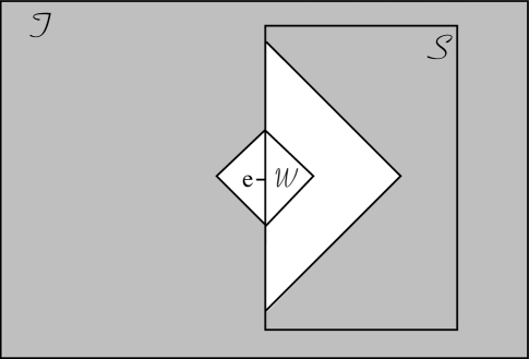
Figure 2. $\mathcal{F}$ is the shaded region. $\mathcal{S}$ is the inner rectangle, and $\mathcal{T}$ is the complement of $\mathcal{S}$ in the full rectangle $\mathcal{R}$. The large triangular region is $\mathcal{S}\cap B_{\mathcal{R}}(e,r)$. The figure is not precisely to scale.

Define

$$g(\rho_{e},\rho_{\mathcal{U}\backslash\mathcal{F}})=P(\omega_{\mathcal{F}\cap\mathcal{S}}=\rho_{\mathcal{F}\cap\mathcal{S}}^{1}\mid\omega_{\mathcal{F}\cap\mathcal{U}}=\rho_{\mathcal{F}\cap\mathcal{U}}^{1},\omega_{\mathcal{U}\backslash\mathcal{F}}=\rho_{\mathcal{U}\backslash\mathcal{F}},\omega_{e}=\rho_{e}).$$

Then by the nature of the $\mathcal{S}$-split measure,

(4.19) $$P_{\mathcal{S}}^{1}(\omega_{e}=1)=\frac{E(\delta_{[\omega_{e}=1]}g\mid\omega_{\mathcal{F}}=\rho_{\mathcal{F}}^{1})}{E(g\mid\omega_{\mathcal{F}}=\rho_{\mathcal{F}}^{1})},$$

where $E$ denotes expectation with respect to $P$. Let $P_{1}=P(\omega_{\mathcal{R}\backslash(\mathcal{F}\cap\mathcal{U})}\in\cdot\mid\omega_{\mathcal{F}\cap\mathcal{U}}=\rho_{\mathcal{F}\cap\mathcal{U}}^{1})$, so that $g(\rho_{e},\rho_{\mathcal{U}\backslash\mathcal{F}})=P_{1}(\omega_{\mathcal{F}\cap\mathcal{S}}=\rho_{\mathcal{F}\cap\mathcal{S}}^{1}\mid\omega_{\mathcal{U}\backslash\mathcal{F}}=\rho_{\mathcal{U}\backslash\mathcal{F}},\omega_{e}=\rho_{e})$. By Proposition 4.2, $\mathfrak{M}^{+}(\mathfrak{S},\mathfrak{R})$ has the ratio strong mixing property, and we would like to apply this property to control the effect of this conditioning of $P_{1}$, but the location $\mathcal{R}\backslash(\mathcal{F}\cap\mathcal{U})=\mathcal{S}\cup\mathcal{W}$ of the configurations under $P_{1}$ need not be in $\mathfrak{S}_{\mathcal{R}}$. However, by Remark 4.3 (with $\mathcal{W}$ or $\mathcal{W}\backslash\mathcal{S}$, whichever is blockable under the admissibility assumption, in place of $\mathcal{E}$) this is not a problem. Thus we have for all $\rho_{e},\rho_{\mathcal{T}\backslash\mathcal{F}}$,

$$\left|\frac{g(\rho_{e},\rho_{\mathcal{T}\backslash\mathcal{F}})}{P_{1}(\omega_{\mathcal{F}\cap\mathcal{S}}=\rho_{\mathcal{F}\cap\mathcal{S}}^{1})}-1\right|\leq c_{27}\sum_{x\in V(\mathcal{T}\backslash\mathcal{F}),y\in V(\mathcal{F}\cap\mathcal{S})}e^{-\lambda d_{\mathcal{R}}(x,y)}\leq c_{28}e^{-\epsilon_{16}r},$$

so that $g$ is nearly a constant in (4.19), and we obtain

$$\left|\frac{P_{\mathcal{S}}^{1}(\omega_{e}=1)}{P(\omega_{e}=1\mid\omega_{\mathcal{F}}=\rho_{\mathcal{F}}^{1})}-1\right|\leq c_{29}e^{-\epsilon_{17}r}.$$

Similarly,

$$\left|\frac{P_{\mathcal{S}}^{0}(\omega_{e}=1)}{P(\omega_{e}=1\mid\omega_{\mathcal{F}}=\rho_{\mathcal{F}}^{0})}-1\right|\leq c_{29}e^{-\epsilon_{17}r}.$$

Next we apply Proposition 4.2 to the collection $\mathfrak{S}_{0}=\{\{\mathcal{R}\}:\mathcal{R}\in\mathfrak{R}\}$, noting that $\mathfrak{M}^{+}(\mathfrak{S}_{0},\mathfrak{R})=\mathfrak{M}$, to obtain

$$\left|\frac{P(\omega_{e}=1\mid\omega_{\mathcal{F}}=\rho_{\mathcal{F}}^{0})}{P(\omega_{e}=1\mid\omega_{\mathcal{F}}=\rho_{\mathcal{F}}^{1})}-1\right|\leq c_{30}e^{-\epsilon_{18}r}.$$

Combining the last 3 inequalities we obtain

$$|P_{\mathcal{S}}^{1}(\omega_{e}=1)-P_{\mathcal{S}}^{0}(\omega_{e}=1)|\leq c_{31}e^{-\epsilon_{19}r},$$

which establishes (4.16). ∎

We now turn to the proof of (4.14). Since $\mathfrak{M}_{w}^{+}(\mathfrak{N},\mathfrak{R})$ has uniform exponential decay of connectivity, it follows easily using the FKG property that if we take the class of balls $\mathfrak{B}=\mathfrak{B}(\mathfrak{R})=\{B_{\mathcal{R}}(x,s):\mathcal{R}\in\mathfrak{R},x\in V(\mathcal{R}),s>1\}$ in place of $\mathfrak{N}$, the class $\mathfrak{M}^{+}(\mathfrak{B},\mathfrak{R})$ has uniform exponential decay as well, that is, there exists $C,\lambda>0$ such that

$$P(x\leftrightarrow y\text{ via a path in }\mathcal{B}\mid\omega_{\mathcal{R}\backslash\mathcal{B}}=\rho_{\mathcal{R}\backslash\mathcal{B}})\leq Ce^{-\lambda d_{\mathcal{R}}(x,y)}$$

for all $\mathcal{R}\in\mathfrak{R}$, all $\mathcal{B}\subset\mathcal{R}$ in $\mathfrak{B}$, all $x,y\in V(\mathcal{B})$ and all boundary conditions $\rho$.

Recall that for (4.14) we have a fixed $\mathcal{R}\in\mathfrak{R}$, a filling sequence $\mathcal{V}=\{b_{1},..,b_{n}\}$ and $\mathcal{S}=\{b_{1},..,b_{k-1}\},e=b_{k}$. Let $m=\lfloor r/24\rfloor$. For $x\in V(\mathcal{R})$ let $\mathcal{Q}_{x}=B_{\mathcal{R}}(x,3m)\cap\mathcal{T}$ and $\mathcal{A}_{x}=\mathcal{R}\backslash B_{\mathcal{R}}(x,3m)$, and for each configuration $\rho_{\mathcal{Q}_{x}}$ let

$$\phi_{x}(\rho_{\mathcal{Q}_{x}})=P\left(x\leftrightarrow y\text{ for some }y\in V(\mathcal{R})\text{ with }d_{\mathcal{R}}(x,y)\geq m\ \Big{|}\ \omega_{\mathcal{Q}_{x}}=\rho_{\mathcal{Q}_{x}},\omega_{\mathcal{A}_{x}}=\rho_{\mathcal{A}_{x}}^{1}\right).$$

Then since $B_{\mathcal{R}}(x,3m)\in\mathfrak{B}$,

(4.20) $$E_{\mathcal{R},w}(\phi_{x}(\omega_{\mathcal{Q}_{x}})) \leq P\left(x\leftrightarrow y\text{ for some }y\in V(\mathcal{R})\text{ with }d_{\mathcal{R}}(x,y)\geq m\ \Big{|}\ \omega_{\mathcal{A}_{x}}=\rho_{\mathcal{A}_{x}}^{1}\right)$$

$$\leq c_{32}m^{d-1}\ Ce^{-\lambda m}.$$

We say that $\mathcal{Q}_{x}$ is connection–inducing in a configuration $\rho_{\mathcal{Q}_{x}}$ if $\phi_{x}(\rho_{\mathcal{Q}_{x}})\geq Ce^{-\lambda m/2}$. Roughly speaking, $\mathcal{Q}_{x}$ is connection-inducing if $\rho_{\mathcal{Q}_{x}}$ either contains a long open path starting in $Q_{m}(x)$, or contains enough segments of such a path that the conditional probability for such a path given $\rho_{\mathcal{Q}_{x}}$ is greatly increased above the unconditional probability. If $\mathcal{Q}_{x}$ is not connection–inducing we say it is insulating. Note that $\phi_{x}$ is an increasing function. Hence using the FKG inequality and (4.20), for every $x$ and $\zeta$,

(4.21) $$P_{\mathcal{R},\zeta}(\mathcal{Q}_{x}\text{ is connection--inducing}) =P_{\mathcal{R},\zeta}(\phi_{x}(\omega_{\mathcal{Q}_{x}})\geq Ce^{-\lambda m/2})$$

$$\leq\frac{E_{\mathcal{R},w}(\phi_{x}(\omega_{\mathcal{Q}_{x}}))}{Ce^{-\lambda m/2}}$$

$$\leq c_{33}e^{-\lambda m/3}.$$

The idea can now be sketched as follows. Recall that $\mathcal{U}=\mathcal{T}\backslash\{e\}$. Suppose $A$ and $B$ occur $(\mathcal{S}\cup\{e\})$-split at separation $r$ in $(\omega_{\mathcal{U}},(1,\omega_{\mathcal{S}}^{1}),(1,\tilde{\omega}_{\mathcal{S}}^{1}))$ with $A$ occurring far from $e$, that is, $(\omega_{\mathcal{U}},\omega_{\mathcal{S}}^{1},\omega_{\mathcal{S}}^{0},\tilde{\omega}_{\mathcal{S}}^{1},\tilde{\omega}_{\mathcal{S}}^{0})\in C_{11}^{A}$, with $A$ occuring on some set $\mathcal{E}$ and $B$ on some set $\mathcal{F}$, with $d_{\mathcal{R}}(e,\mathcal{E})\geq r/3$. Since $P$ has the FKG property and the Markov property for blocking sets, the FKG couplings $\hat{P}_{\zeta_{\mathcal{U}}},\zeta_{\mathcal{U}}\in\{0,1\}^{\mathcal{U}}$, of the two layers of the $A$ pair can be chosen so that $\omega_{\mathcal{S}}^{1}=\omega_{\mathcal{S}}^{0}$ outside $C_{e}=C_{e}((\zeta_{\mathcal{U}},1,\omega_{\mathcal{S}}^{1}))$, which is the cluster of $e$ for the top layer together with the unsplit bonds. (The construction of such couplings is standard–see e.g. [8], [23].) Suppose now that the $A$ pair fails to couple on $\mathcal{E}$, that is, $\omega_{\mathcal{E}\cap\mathcal{S}}^{1}\neq\omega_{\mathcal{E}\cap\mathcal{S}}^{0}$. This means that the cluster $C_{e}$ intersects $\mathcal{E}$, i.e. there is an open path from $e$ to $\mathcal{E}$ in the top layer of the $A$ pair. Since $d(\mathcal{E},\mathcal{F})\geq r$, a segment of this path is far from $\mathcal{E},\mathcal{F}$ and $e$. This segment may be partly in $\mathcal{U}$ and partly in $\mathcal{S}$. There are two possibilities: either the segment is substantially helped to exist by some connection-inducing region of $\mathcal{U}$, or the portion in $\mathcal{S}$ exists without such help, that is, the relevant regions of $\mathcal{U}$ are insulating. The first is exponentially unlikely, even conditionally on the occurrence of $A\circ_{r,\mathcal{S}}B$ on $\mathcal{E}\cup\mathcal{F}$ in the top layers of the $A$ and $B$ pairs, by Proposition 4.1. The second is also (conditionally) exponentially unlikely, by the definition of insulating and the ratio strong mixing property.

Turning to the details, we let $D_{11}^{A}$ denote the set of all $(\omega_{\mathcal{U}},\omega_{\mathcal{S}}^{1},\omega_{\mathcal{S}}^{0},\tilde{\omega}_{\mathcal{S}}^{1},\tilde{\omega}_{\mathcal{S}}^{0})$ such that there exist $\mathcal{E},\mathcal{F}$ for which $A$ and $B$ occur $(\mathcal{S}\cup\{e\})$-split at separation $r$ (which is at least $24m$) in $(\omega_{\mathcal{U}},(1,\omega_{\mathcal{S}}^{1}),(1,\tilde{\omega}_{\mathcal{S}}^{1}))$, i.e. using the two top layers, with $A$ occuring on $\mathcal{E}$, $B$ occurring on $\mathcal{F}$, $d_{\mathcal{R}}(e,\mathcal{E})>8m$, and $\omega_{\mathcal{E}}^{1}\neq\omega_{\mathcal{E}}^{0}$, and for some $z\in V(\mathcal{D}^{r}(\mathcal{R}))$, we have that $\mathcal{Q}_{z}$ is connection-inducing, $d_{\mathcal{R}}(z,e)>3m$ and $d_{\mathcal{R}}(z,\mathcal{E}\cup\mathcal{F})>4m$. Let $E_{11}^{A}$ be the set of all $(\omega_{\mathcal{U}},\omega_{\mathcal{S}}^{1},\omega_{\mathcal{S}}^{0},\tilde{\omega}_{\mathcal{S}}^{1},\tilde{\omega}_{\mathcal{S}}^{0})$ such that there exist $\mathcal{E},\mathcal{F}$ for which $A$ and $B$ occur $(\mathcal{S}\cup\{e\})$-split at separation $r$ in $(\omega_{\mathcal{U}},(1,\omega_{\mathcal{S}}^{1}),(1,\tilde{\omega}_{\mathcal{S}}^{1}))$ with $A$ occuring on $\mathcal{E}$, $B$ occurring on $\mathcal{F}$, $d_{\mathcal{R}}(e,\mathcal{E})>8m$, and $\omega_{\mathcal{E}}^{1}\neq\omega_{\mathcal{E}}^{0}$, but for no choice of such $\mathcal{E},\mathcal{F}$ does there exist $z$ as above. $D_{11}^{B}$ and $E_{11}^{B}$ are defined analogously. Then

$$C_{11}^{A}\backslash(C_{01}\cup C_{10})\subset D_{11}^{A}\cup E_{11}^{A},$$

and similarly with $B$in place of $A$. Therefore provided $c_{7}$ is sufficiently large, by Proposition 4.1 and (4.21),

(4.22) $$\mathbb{P}_{\mathcal{S},e} ((\omega_{\mathcal{U}},\omega_{\mathcal{S}}^{1},\omega_{\mathcal{S}}^{0},\tilde{\omega}_{\mathcal{S}}^{1},\tilde{\omega}_{\mathcal{S}}^{0})\in D_{11}^{A},\omega_{e}=\tilde{\omega}_{e}=1)$$

$$\leq\sum_{z\in V(\mathcal{D}^{r}(\mathcal{R})):d_{\mathcal{R}}(z,e)>3m}\mathbb{P}_{\mathcal{S},e}\Bigl{(}\omega_{e}=\tilde{\omega}_{e}=1,\mathcal{Q}_{z}\text{ is connection-inducing in }(\omega_{\mathcal{U}},1),$$

$$\qquad\qquad\qquad\qquad\qquad\qquad A\circ_{r,\mathcal{S}}B\text{ occurs on }B_{\mathcal{R}}(z,4m)^{c})\text{ in }(\omega_{\mathcal{U}},(1,\omega_{\mathcal{S}}^{1}),(1,\tilde{\omega}_{\mathcal{S}}^{1}))\Bigr{)}$$

$$\leq\sum_{z\in V(\mathcal{V})}P_{\mathcal{S}}(A\circ_{r,\mathcal{S}}B)\cdot\Bigl{(}\mathbb{P}_{\mathcal{S},e}\bigl{(}\mathcal{Q}_{z}\text{ is connection-inducing }\bigr{)}$$

$$\qquad\qquad\qquad\qquad\qquad\qquad\qquad\qquad+C\sum_{x\in V(B_{\mathcal{R}}(z,3m)),y\in V(B_{\mathcal{R}}(z,4m)^{c}))}e^{-\lambda d_{\mathcal{R}}(x,y)}\Bigr{)}$$

$$\leq c_{34}|\mathcal{V}|e^{-\epsilon_{20}r}P_{\mathcal{S}}(A\circ_{r,\mathcal{S}}B)$$

$$\leq c_{35}e^{-\epsilon_{21}r}P_{\mathcal{S}}(A\circ_{r,\mathcal{S}}B).$$

Here we have used the fact that when $d_{\mathcal{R}}(z,e)>3m$ we have $e\notin\mathcal{Q}_{z}$, so whether or not $\mathcal{Q}_{z}$ in connection-inducing in $(\omega_{\mathcal{U}},\omega_{e})$ does not depend on $\omega_{e}$. Next, let $H_{z}$ denote the event that $z\leftrightarrow y\text{ in }(\omega_{\mathcal{U}},1,\omega_{\mathcal{S}}^{1})$ for some $y$ with $|y-z|\geq m$, $I_{z}$ the event that $\mathcal{Q}_{z}$ is insulating in $(\omega_{\mathcal{U}},1)$ and $J_{z}$ the event that $A\circ_{r,\mathcal{S}}B$ occurs on $B_{\mathcal{R}}(z,4m)^{c}$ in $(\omega_{\mathcal{U}},(1,\omega_{\mathcal{S}}^{1}),(1,\tilde{\omega}_{\mathcal{S}}^{1}))$. Observe that if $(\omega_{\mathcal{U}},\omega_{\mathcal{S}}^{1},\omega_{\mathcal{S}}^{0},\tilde{\omega}_{\mathcal{S}}^{1},\tilde{\omega}_{\mathcal{S}}^{0})\in E_{11}^{A}$ then there is an open path from $e$ to $\mathcal{E}$ in the top layer of the $A$ pair, and this path must path through a site $z$ at $d_{\mathcal{R}}$-distance approximately $4m$ from $\mathcal{E}$; this forces the event $H_{z}\cap I_{z}\cap J_{z}$ to occur. (Here we use the fact that $\omega_{\mathcal{S}}^{1}=\omega_{\mathcal{S}}^{0}$ outside $C_{e}$.) Hence using the conditional independence inherent in the $\mathcal{S}$-split structure,

(4.23) $$\mathbb{P}_{\mathcal{S},e} ((\omega_{\mathcal{U}},\omega_{\mathcal{S}}^{1},\omega_{\mathcal{S}}^{0},\tilde{\omega}_{\mathcal{S}}^{1},\tilde{\omega}_{\mathcal{S}}^{0})\in E_{11}^{A},\omega_{e}=\tilde{\omega}_{e}=1)$$

$$\leq\sum_{z\in V(\mathcal{D}^{r}(\mathcal{R})):d_{\mathcal{R}}(z,e)>3m}\mathbb{P}_{\mathcal{S},e}(H_{z}\cap I_{z}\cap J_{z},\omega_{e}=1)$$

$$\leq\sum_{z\in V(\mathcal{D}^{r}(\mathcal{R})):d_{\mathcal{R}}(z,e)>3m}\ \sum_{\zeta_{\mathcal{U}}\in I_{z}}\mathbb{P}_{\mathcal{S},e}(J_{z},\omega_{e}=1,\omega_{\mathcal{U}}=\zeta_{\mathcal{U}})\mathbb{P}_{\mathcal{S},e}(H_{z}\mid J_{z},\omega_{e}=1,\omega_{\mathcal{U}}=\zeta_{\mathcal{U}}).$$

From the definition of insulating and the FKG property we have

$$\mathbb{P}_{\mathcal{S},e}(H_{z}\mid J_{z},\omega_{e}=1,\omega_{\mathcal{U}}=\zeta_{\mathcal{U}})<Ce^{-\lambda m/2},$$

so (4.23) yields

(4.24) $$\mathbb{P}_{\mathcal{S},e} ((\omega_{\mathcal{U}},\omega_{\mathcal{S}}^{1},\omega_{\mathcal{S}}^{0},\tilde{\omega}_{\mathcal{S}}^{1},\tilde{\omega}_{\mathcal{S}}^{0})\in E_{11}^{A},\omega_{e}=\tilde{\omega}_{e}=1)$$

$$\leq\sum_{z\in V(\mathcal{V})}Ce^{-\lambda m/2}\ \mathbb{P}_{\mathcal{S},e}(J_{z},\omega_{e}=1)$$

$$\leq c_{36}|\mathcal{V}|e^{-\lambda m/2}P_{\mathcal{S}}(A\circ_{r,\mathcal{S}}B)$$

$$\leq c_{37}e^{-\epsilon_{22}r}P_{\mathcal{S}}(A\circ_{r,\mathcal{S}}B).$$

Now (4.22) and (4.24) show that

$$\mathbb{P}_{\mathcal{S},e}\Bigl{(}(\omega_{\mathcal{U}},\omega_{\mathcal{S}}^{1},\omega_{\mathcal{S}}^{0},\tilde{\omega}_{\mathcal{S}}^{1},\tilde{\omega}_{\mathcal{S}}^{0})\in C_{11}^{A}\backslash(C_{01}\cup C_{10}),\omega_{e}=\tilde{\omega}_{e}=1\Bigr{)}\leq c_{38}e^{-\epsilon_{23}r}P_{\mathcal{S}}(A\circ_{r,\mathcal{S}}B)$$

and a similar bound holds for $C_{11}^{B}$, so we have established (4.14), and thus also (4.1) and then (4.2). This proves Theorem 3.1.

Proof of Theorem 3.2..

Let $\mathfrak{R},\mathfrak{S},\mathfrak{V},\mathfrak{M},\mathfrak{N}$ be as in Example 1.2.

Suppose first that $\rho$ is wired or all external fields are 0. As noted in Example 1.2, $(\mathfrak{R},\mathfrak{S},\mathfrak{V},$ $\mathfrak{M},\mathfrak{N})$ is then filling-compatible. All finite-volume measures $P_{\mathcal{B},\rho}$, with $\mathcal{B}$ finite and $\rho$ a bond boundary condition, satisfy the FKG lattice condition ([13]; see [2]). It follows that $P$ has uniform exponential decay of connectivity for the class $\overline{\mathfrak{R}}$ with arbitrary bond boundary conditions, not just wired. By Lemma 2.1, since the set $\mathcal{R}\backslash\mathcal{S}$ is connected and abuts $\mathcal{R}^{c}$ for all $\mathcal{R}\in\mathfrak{R}$ and $\mathcal{S}\in\mathfrak{S}_{\mathcal{R}}$, every measure in $\mathfrak{M}\ \cup\ \mathfrak{M}^{+}(\mathfrak{S},\mathfrak{R})$ has the Markov property for blocking sets. Thus in this case (i) follows from Theorem 3.1.

For the remaining case, suppose $\rho$ is free and not all external fields are 0. Consider a measure $Q=P_{\mathcal{R},f}(\omega_{\mathcal{S}}\in\cdot\mid\omega_{\mathcal{R}\backslash\mathcal{S}}=\rho_{\mathcal{R}\backslash\mathcal{S}}^{1})\in\mathfrak{M}^{+}(\mathfrak{S},\mathfrak{R})$. As we have noted, $\mathcal{R}\backslash\mathcal{S}$ is connected so the effective boundary condition on $\mathcal{S}$ given by $Q$ is a unique-cluster one. Let $(\mathcal{X},\mathcal{Y},\mathcal{Z})$ be a blocking partition of $\mathcal{S}$, and suppose $\omega=0$ on $\mathcal{Y}$. We use the notation of the proof of Lemma 2.1. Note that the set of bonds in $C_{u}$ is $\mathcal{R}\backslash\mathcal{S}$. The factoring of the weight of a cluster $\hat{C}$ described in that proof is not necessarily valid; the clusters $C_{i}$ effectively interact via the value $s(\hat{C})$. More precisely, conditionally on $\{C_{j},j\neq i\}$, the effective weight attached to $C_{i}$ depends on $s(C_{u})+\sum_{j\neq i}s(C_{j})$; since some $C_{m}$’s may be in $\mathcal{X}$ and others in $\mathcal{Z}$, this means the Markov property for blocking sets need not hold. However, letting $h_{k}$ be the largest strictly negative external field, the effective weight of $C_{i}$ is always between 1 and $1+O(e^{-c|h_{k}|s(C_{u})})$, that is, the maximum influence of $\{C_{j},j\neq i\}$ on $C_{i}$ is exponentially small in $s(C_{u})$. Roughly speaking, we have two situations. If $s(C_{u})$ is small relative to $r$ then since $\operatorname{diam}_{\mathcal{R}}(C_{u})\leq s(C_{u})$ the interaction between clusters $C_{i}$ of $\omega$ only occurs over length scales which are small relative to $r$. If $s(C_{u})$ is of order $r$ or greater, then the above-mentioned maximum influence of $\{C_{j},j\neq i\}$ on $C_{i}$ is exponentially small in $r$. Either way, though we do not fully have the Markov property for blocking sets, the proofs of Proposition 4.1, Example 1.2 and then Theorem 3.1 go through; we omit the full details. See ([3], Lemma 2.11(iii)) for a similar result. Thus (i) is proved in all cases.

For (ii) let $\mathcal{B}_{n}=\mathcal{B}([-n,n]^{d})$ and let $A_{n}$ be the event that $A$ occurs on $\mathcal{B}_{n}$. By the uniform exponential decay assumption, $P$ is the unique infinite-volume random cluster measure at $(p,q,\{h_{i}\})$. Therefore by (i),

$$P(A_{n}\circ_{r}B) =\lim_{m}P_{\mathcal{B}_{m},w}(A_{n}\circ_{r}B)$$

$$\leq(1+c_{9}e^{-\epsilon_{5}r})\lim_{m}P_{\mathcal{B}_{m},w}(A_{n})P_{\mathcal{B}_{m},w}(B)$$

$$=(1+c_{9}e^{-\epsilon_{5}r})P(A_{n})P(B).$$

Since $A$ is locally-occurring we can now take a limit as $n\to\infty$ to obtain (ii). ∎

Proof of Theorem 3.4..

Let $\mathfrak{S}_{\mathcal{R}},\mathfrak{N}$ and $\mathfrak{M}$ be as in Example 1.3. Since $d=2$, uniform exponential decay of connectivity for the class $\mathfrak{M}^{+}(\mathfrak{S},\mathfrak{R})$ with wired boundary conditions follows from the assumed infinite-volume exponential decay [3]. As we have noted, all finite-volume measures $P_{\mathcal{B},\rho}$, with $\mathcal{B}$ finite and $\rho$ a bond boundary condition, satisfy the FKG lattice condition ([13]; see [2]). We consider the case in which the boundary is wired ($i=1$) or there are no external fields; the case of free boundary with external fields can be handled as in the proof of Theorem 3.2. Example 1.3 establishes filling-compatibility of $(\mathfrak{R},\mathfrak{V},\mathfrak{S},\mathfrak{M},\mathfrak{N})$. The Markov property for blocking sets for $\mathfrak{M}\cup\mathfrak{M}^{+}(\mathfrak{S},\mathfrak{N})$ follows from Lemma 2.1. The theorem now follows from Theorem 3.1. ∎

We write $\operatorname{Int}(\gamma)$ and $\operatorname{Ext}(\gamma)$ for the interior and exterior of a simple closed curve $\gamma$ in the plane.

Proof of Theorem 3.6..

For a configuration $\omega$ on $\mathcal{R}$ we define the boundary cluster $C_{\partial}(\omega)$ to be the set of open bonds which are connected to $V(\mathcal{R}^{c})$ by a path of open bonds. (This is a mild abuse of terminology since $C_{\partial}$ does not necessarily consist of a single connected cluster.) Then $(\partial C_{\partial})^{*}$ includes a finite collection of open dual circuits; these circuits have disjoint interiors. Let $\mathfrak{D}=\mathfrak{D}(\omega)$ be the set of dual circuits in this collection which contain bonds of $\mathcal{D}^{*}$. Let $\mathcal{I}=\mathcal{I}(\mathfrak{D}(\omega))=\cup_{\gamma\in\mathfrak{D}}\ \mathcal{B}(\operatorname{Int}(\gamma)),\mathcal{J}=\mathcal{J}(\mathfrak{D}(\omega))=\cap_{\gamma\in\mathfrak{D}}\ \mathcal{B}(\operatorname{Ext}(\gamma))$. Conditionally on $[\mathfrak{D}=\mathbb{D}]$ for some $\mathbb{D}$, the configuration on $\mathcal{I}(\mathbb{D})$ is a free-boundary FK configuration. Let $I_{AB}$ denote the event that $A\circ_{r}B$ occurs with $B$ occuring on $\mathcal{I}$ at distance $r/4$ or more from $\mathcal{I}^{c}$, that is, there exist $\mathcal{E}\subset\mathcal{R},\mathcal{F}\subset\mathcal{I}\cap\mathcal{D}$ with $d(\mathcal{E},\mathcal{F})\geq r,d(\mathcal{F},\mathcal{I}^{c})\geq r/4$ such that $A$ occurs on $\mathcal{E}$ and $B$ occurs on $\mathcal{F}$. Let $G_{x}$ be the event that there is an open path in $\mathcal{R}$ from $x$ to $y$ for some $y\in V(\mathcal{R})$ with $d_{\mathcal{R}}(x,y)\geq r/4$.

Suppose $\omega\in(A\circ_{r}B)\backslash I_{AB}$, with $A,B$ occuring on $\mathcal{E},\mathcal{F}$ respectively. Then there is an open path from the boundary $V(\mathcal{R}^{c})\cap V(\mathcal{R})$ to $\mathcal{F}^{r/4}$, and since $d(\mathcal{E},\mathcal{F})\geq r$ a portion of length $r/4$ of this path must be separated from both $\mathcal{E}$ and $\mathcal{F}$ by a distance of more than $r/4$. More precisely, for some $x\in V(\mathcal{D}^{r})$ on this path at distance approximately $r/2$ from $\mathcal{F}$ we have $\omega\in G_{x}\cap H_{x}$, where $H_{x}$ is the event that $A\circ_{r}B$ occurs on $\mathcal{R}\backslash B_{\mathcal{R}}(x,3r/8)$. Therefore using the FKG property,

(4.25) $$P_{\mathcal{R},\rho}\bigl{(}(A\circ_{r}B)\backslash I_{AB}\bigr{)} \leq\sum_{x\in V(\mathcal{D}^{r})}P_{\mathcal{R},\rho}(G_{x}\mid H_{x})P_{\mathcal{R},\rho}(H_{x})$$

$$\leq P_{\mathcal{R},\rho}(A\circ_{r}B)\sum_{x\in V(\mathcal{D}^{r})}P_{B_{\mathcal{R}}(x,3r/8),w}(G_{x}).$$

Since $P$ has exponential decay of connectivity, it has uniform exponential decay for the class of all SLC subsets [3] and therefore

$$P_{B_{\mathcal{R}}(x,3r/8),w}(G_{x})\leq c_{39}e^{-\epsilon_{24}r}.$$

Thus provided $c_{11}$ is large enough we have

(4.26) $$P_{\mathcal{R},\rho}\bigl{(}(A\circ_{r}B)\backslash I_{AB}\bigr{)}\leq c_{40}e^{-\epsilon_{25}r}P_{\mathcal{R},\rho}(A\circ_{r}B).$$

Next we bound $P_{\mathcal{R},\rho}(I_{AB})$. Given $\mathcal{B}\subset\mathcal{R}$ and a configuration $\zeta_{\mathcal{R}\backslash\mathcal{B}}$ on $\mathcal{R}\backslash\mathcal{B}$, let

$$A(\zeta_{\mathcal{R}\backslash\mathcal{B}})=\{\zeta_{\mathcal{B}}:(\zeta_{\mathcal{R}\backslash\mathcal{B}}\zeta_{\mathcal{B}})\in A\}.$$

Next let $\mathcal{I}_{r/4}(\mathbb{D})=\{b\in\mathcal{I}(\mathbb{D}),d(b,\mathbb{D})\geq r/4\}$ and let $B(\mathbb{D})$ be the event that $B$ occurs on $\mathcal{I}_{r/4}(\mathbb{D})$. We have

(4.27) $$P_{\mathcal{R},\rho}(I_{AB}) \leq\sum_{\mathbb{D}}\sum_{\zeta_{\mathcal{J}(\mathbb{D})}}P_{\mathcal{R},\rho}\bigl{(}I\mid\mathfrak{D}=\mathbb{D},\omega_{\mathcal{J}(\mathbb{D})}=\zeta_{\mathcal{J}(\mathbb{D})}\bigr{)}P_{\mathcal{R},\rho}\bigl{(}\mathfrak{D}=\mathbb{D},\omega_{\mathcal{J}(\mathbb{D})}=\zeta_{\mathcal{J}(\mathbb{D})}\bigr{)}$$

$$=\sum_{\mathbb{D}}\sum_{\zeta_{\mathcal{J}(\mathbb{D})}}P_{\mathcal{I}(\mathbb{D}),f}(A(\zeta_{\mathcal{J}(\mathbb{D})}\rho^{0}_{\mathbb{D}})\circ_{r}B(\mathbb{D}))P_{\mathcal{R},\rho}\bigl{(}\mathfrak{D}=\mathbb{D},\omega_{\mathcal{J}(\mathbb{D})}=\zeta_{\mathcal{J}(\mathbb{D})}\bigr{)}.$$

We would like to apply Theorem 3.4 to the first probability on the right side of (4.27), but $\mathcal{I}(\mathbb{D})$ need not be a circuit-bounded set. However, for each connected component $G$ of the interior of $\mathcal{I}(\mathbb{D})^{\operatorname{solid}}$, $\mathcal{B}(\overline{G})$ is circuit-bounded, the relevant circuit being the boundary of $G$. We let $\mathcal{I}_{\operatorname{main}}(\mathbb{D})$ denote the union of all such $\mathcal{B}(\overline{G})$. Then $\mathcal{I}_{\operatorname{main}}(\mathbb{D})$ is a finite union of circuit-bounded sets, and $d_{\mathcal{R}}(\mathcal{I}_{\operatorname{main}}(\mathbb{D})^{c},\mathcal{I}_{r/4}(\mathbb{D}))\geq r/4$. Since $\mathcal{I}(\mathbb{D})$ has SLC components, for each $\mathcal{B}(\overline{G})$, each connected component of $\mathcal{I}(\mathbb{D})\backslash\mathcal{B}(\overline{G})$ can intersect $\mathcal{B}(\overline{G})$ in at most a single site. This means that under a free boundary condition on $\mathcal{I}(\mathbb{D})$, for each $\overline{G}$, regardless of the configuration on $\mathcal{I}(\mathbb{D})\backslash\mathcal{B}(\overline{G})$, the effective boundary condition on $\mathcal{B}(\overline{G})$ is free. Therefore

(4.28) $$P_{\mathcal{I}(\mathbb{D}),f} (A(\zeta_{\mathcal{J}(\mathbb{D})}\rho^{0}_{\mathbb{D}})\circ_{r}B(\mathbb{D}))$$

$$=\sum_{\zeta_{\mathcal{I}(\mathbb{D})\backslash\mathcal{I}_{\operatorname{main}}(\mathbb{D})}}P_{\mathcal{I}_{\operatorname{main}}(\mathbb{D}),f}\bigl{(}A(\zeta_{\mathcal{J}(\mathbb{D})}\rho^{0}_{\mathbb{D}}\zeta_{\mathcal{I}(\mathbb{D})\backslash\mathcal{I}_{\operatorname{main}}(\mathbb{D})})\circ_{r}B(\mathbb{D})\bigr{)}$$

$$\qquad\qquad\qquad\qquad\cdot P_{\mathcal{I}(\mathbb{D}),f}(\omega_{\mathcal{I}(\mathbb{D})\backslash\mathcal{I}_{\operatorname{main}}(\mathbb{D})}=\zeta_{\mathcal{I}(\mathbb{D})\backslash\mathcal{I}_{\operatorname{main}}(\mathbb{D})})$$

By Theorem 3.4 and Remark 3.5 we have

(4.29) $$P_{\mathcal{I}_{\operatorname{main}}(\mathbb{D}),f} \bigl{(}A(\zeta_{\mathcal{J}(\mathbb{D})}\rho^{0}_{\mathbb{D}}\zeta_{\mathcal{I}(\mathbb{D})\backslash\mathcal{I}_{\operatorname{main}}(\mathbb{D})})\circ_{r}B(\mathbb{D})\bigr{)}$$

$$\leq(1+c_{12}e^{-\epsilon_{6}r})P_{\mathcal{I}_{\operatorname{main}}(\mathbb{D}),f}(A(\zeta_{\mathcal{J}(\mathbb{D})}\rho^{0}_{\mathbb{D}}\zeta_{\mathcal{I}(\mathbb{D})\backslash\mathcal{I}_{\operatorname{main}}(\mathbb{D})}))P_{\mathcal{I}_{\operatorname{main}}(\mathbb{D}),f}(B(\mathbb{D})).$$

Since $P$ has exponential decay of connectivity, it has uniform exponential decay for the class of all SLC subsets [3] and therefore by Proposition 4.1,

(4.30) $$P_{\mathcal{I}_{\operatorname{main}}(\mathbb{D}),f}(B(\mathbb{D}))\leq(1+c_{41}e^{-\epsilon_{26}r})P_{\mathcal{R},\rho}(B(\mathbb{D}))\leq(1+c_{37}e^{-\epsilon_{26}r})P_{\mathcal{R},\rho}(B).$$

Combining (4.27)–(4.30) we obtain

(4.31) $$P_{\mathcal{R},\rho} (I_{AB})$$

$$\leq(1+c_{42}e^{-\epsilon_{27}r})P_{\mathcal{R},\rho}(B)$$

$$\qquad\cdot\sum_{\mathbb{D}}\sum_{\zeta_{\mathcal{J}(\mathbb{D})}}\sum_{\zeta_{\mathcal{I}(\mathbb{D})\backslash\mathcal{I}_{\operatorname{main}}(\mathbb{D})}}P_{\mathcal{I}_{\operatorname{main}}(\mathbb{D}),f}(A(\zeta_{\mathcal{J}(\mathbb{D})}\rho^{0}_{\mathbb{D}}\zeta_{\mathcal{I}(\mathbb{D})\backslash\mathcal{I}_{\operatorname{main}}(\mathbb{D})}))$$

$$\qquad\qquad\qquad\qquad\cdot P_{\mathcal{R},\rho}\bigl{(}\mathfrak{D}=\mathbb{D},,\omega_{\mathcal{J}(\mathbb{D})}=\zeta_{\mathcal{J}(\mathbb{D})},\omega_{\mathcal{I}(\mathbb{D})\backslash\mathcal{I}_{\operatorname{main}}(\mathbb{D})}=\zeta_{\mathcal{I}(\mathbb{D})\backslash\mathcal{I}_{\operatorname{main}}(\mathbb{D})}\bigr{)}$$

$$=(1+c_{42}e^{-\epsilon_{27}r})P_{\mathcal{R},\rho}(B)P_{\mathcal{R},\rho}(A).$$

This and (4.26) complete the proof. ∎

The proof of Theorem 3.7 is generally similar to that of Theorem 3.1, except that the couplings of the top and bottom layers are obtained by a different construction. We will need two lemmas to replace Proposition 4.2.

Lemma 4.4.

[3] Let $\mu^{\beta,h}$ be the Ising model at $(\beta,h)$ on $\mathbb{Z}^{d}$, with $\beta<\beta_{c}(d,h)$. Let $\mathfrak{L}$ be a class of subsets of $\mathbb{Z}^{d}$ which has the neighborhood component property. Suppose that the corresponding FK model has uniform exponential decay of finite-volume connectivities for the class $\{\mathcal{B}(\Lambda):\Lambda\in\mathfrak{L}\}$ with wired boundary conditions. Then $\mu^{\beta,h}$ has the ratio strong mixing property for the class $\mathfrak{L}$ and arbitrary boundary conditions.

Lemma 4.5.

Let $\mu^{\beta,h}$ be the Ising model at $(\beta,h)$ on $\mathbb{Z}^{2}$ and let $\mathfrak{L}$ be the class of all finite SLC subsets of $\mathbb{Z}^{2}$ with arbitrary boundary condition. Suppose that either (a) $\beta<\beta_{c}(2,0)$ and $h=0$, (b) $\beta>\beta_{c}(2,0)$ and $h\neq 0$, (c) $\beta<\beta_{c}(2,h)$ and the corresponding FK model has exponential decay of connectivities (in infinite volume), or (d) $\beta>\beta_{c}(2,h)$ and the corresponding FK model has exponential decay of dual connectivities (in infinite volume). Then $\mu^{\beta,h}$ has the ratio strong mixing property for the class $\mathfrak{L}$.

Proof.

Under (c) and (d) this is proved in [3]. Suppose (a) holds; then the Ising model has exponential decay of correlations [1], so by 2.5 the corresponding FK model has exponential decay of connectivities, and (a) follows from (c). Next suppose (b) holds; we may assume $h>0$. The Ising model then FKG-dominates the plus phase at $(\beta,0)$. In the plus phase at $(\beta,0)$, the probability that there is a path from 0 to $x$ on which all sites $y$ have $\sigma_{y}=-1$ decays exponentially in $|x|$ [10], so the same is true at $(\beta,h)$. It follows that the corresponding ARC model (an alternate graphical representation of the Ising model—see [5]) at $(\beta,h)$ has exponential decay of connectivities (in infinite volume), which in turn implies that $\mu^{\beta,h}$ has the ratio strong mixing property for the class $\mathfrak{L}$ [3]. ∎

It is plausible that the exponential decay assumptions in Lemma 4.5(c) and (d) are valid for all $\beta$ below and above $\beta_{c}(2,h)$, respectively, but this is not known rigorously for all $h\neq 0$.

We next construct the coupling that will be used in the $A$ and $B$ pairs for the Ising model.

Lemma 4.6.

Suppose $\mu$ is an Ising model on $\mathbb{Z}^{d}$ having the ratio strong mixing property for some class $\mathfrak{L}$ of finite subsets of $\mathbb{Z}^{d}$ with arbitrary boundary conditions. There exist $c_{i},\epsilon_{i}$ as follows. Suppose $\Delta\subset\Lambda\subset\mathbb{Z}^{d}$ with $\Lambda\in\mathfrak{L}$, $\alpha\in\{-1,1\}^{\partial\Lambda}$, $r\geq c_{43}\log|\Delta|$, and $\eta_{\Delta}\geq\eta_{\Delta}^{\prime}\in\{-1,1\}^{\Delta}$. There exists an FKG coupling $\hat{\mu}_{\Lambda,\alpha}$ of $\mu_{\Lambda,\alpha}(\sigma_{\Lambda\backslash\Delta}\in\cdot\mid\sigma_{\Delta}=\eta_{\Delta})$ and $\mu_{\Lambda,\alpha}(\sigma_{\Lambda\backslash\Delta}\in\cdot\mid\sigma_{\Delta}=\eta_{\Delta}^{\prime})$ with the property that

(4.32) $$\hat{\mu}_{\Lambda,\alpha}\bigl{(}\bigl{\{}(\sigma_{\Lambda\backslash\Delta},\sigma_{\Lambda\backslash\Delta}^{\prime}):\sigma_{x}\neq\sigma^{\prime}_{x}\text{ for some }x\in\Lambda\backslash\Delta^{r}(\Lambda)\bigr{\}}\mid\sigma_{\Lambda\backslash\Delta^{r}(\Lambda)}=\eta_{\Lambda\backslash\Delta^{r}(\Lambda)}\bigr{)}$$

$$\qquad\leq c_{44}e^{-\epsilon_{28}r}\quad\text{for every }\eta_{\Lambda\backslash\Delta^{r}(\Lambda)}\in\{-1,1\}^{\Lambda\backslash\Delta^{r}(\Lambda)}.$$

If it were not for the conditioning on $\sigma_{\Lambda\backslash\Delta^{r}(\Lambda)}=\eta_{\Lambda\backslash\Delta^{r}(\Lambda)}$, Lemma 4.6 would be a standard result saying that there is at most an exponentially small probability that the two coupled configurations, given $\eta_{\Delta}$ and given $\eta_{\Delta^{\prime}}$, are unequal far from $\Delta$. This standard result leaves open the possibility, though, that there are a few rare “hard-to-couple-to” configurations $\eta_{\Lambda\backslash\Delta}$ which greatly increase the probability of unequal configurations when they occur, say, in the top layer of the coupled configuration. Lemma 4.6 rules out this possibility.

Lemma 4.6 extends straightforwardly to any bond or site model having the ratio strong mixing property. If the model lacks the FKG property, the coupling will not be an FKG coupling in general.

We will refer to a coupling of the type guaranteed by Lemma 4.6 as an RSM coupling.

Proof of Lemma 4.6.

Let $\Lambda_{\operatorname{far}}=\Lambda\backslash\Delta^{r}(\Lambda)$ and $\Lambda_{\operatorname{near}}=\Delta^{r}(\Lambda)\backslash\Delta$; we will refer to configurations on $\Lambda_{\operatorname{far}}$ and $\Lambda_{\operatorname{near}}$ as far and near configurations, respectively. Define a measure $\nu$ on far configurations by

$$\nu(\zeta_{\Lambda_{\operatorname{far}}})=\min\bigl{(}\mu_{\Lambda,\alpha}(\sigma_{\Lambda_{\operatorname{far}}}=\zeta_{\Lambda_{\operatorname{far}}}\mid\sigma_{\Delta}=\eta_{\Delta}),\mu_{\Lambda,\alpha}(\sigma_{\Lambda_{\operatorname{far}}}=\zeta_{\Lambda_{\operatorname{far}}}\mid\sigma_{\Delta}=\eta_{\Delta}^{\prime})\bigr{)},$$

and let

$$\nu_{0}=\nu\left(\{-1,1\}^{\Lambda_{\operatorname{far}}}\right),$$

$$\tau(\cdot)=\frac{\mu_{\Lambda,\alpha}(\sigma_{\Lambda_{\operatorname{far}}}\in\cdot\mid\sigma_{\Delta}=\eta_{\Delta})-\nu(\cdot)}{1-\nu_{0}},\qquad\tau^{\prime}(\cdot)=\frac{\mu_{\Lambda,\alpha}(\sigma_{\Lambda_{\operatorname{far}}}\in\cdot\mid\sigma_{\Delta}=\eta_{\Delta}^{\prime})-\nu(\cdot)}{1-\nu_{0}}.$$

We may assume $\nu_{0}<1$, since otherwise the two measures to be coupled are identical. Then $\nu/\nu_{0},\tau$ and $\tau^{\prime}$ are probability measures,

(4.33) $$\min\bigl{(}\tau(\zeta_{\Lambda_{\operatorname{far}}}),\tau^{\prime}(\zeta_{\Lambda_{\operatorname{far}}})\bigr{)}=0\quad\text{for all }\zeta_{\Lambda_{\operatorname{far}}},$$

and by the ratio strong mixing property,

(4.34) $$(1-\nu_{0})\max\left(\frac{\tau(\zeta_{\Lambda_{\operatorname{far}}})}{\nu(\zeta_{\Lambda_{\operatorname{far}}})},\frac{\tau^{\prime}(\zeta_{\Lambda_{\operatorname{far}}})}{\nu(\zeta_{\Lambda_{\operatorname{far}}})}\right)\leq c_{45}e^{-\epsilon_{29}r}\qquad\text{ for all }\zeta_{\Lambda_{\operatorname{far}}}.$$

Let $(\chi,\chi^{\prime}),\xi$ and $X$ be independent, with $\operatorname{Pr}(X=1)=\nu_{0},\operatorname{Pr}(X=0)=1-\nu_{0}$, with $\xi$ having distribution $\nu/\nu_{0}$, and with $(\chi,\chi^{\prime})$ having as its distribution an FKG coupling of $\tau$ and $\tau^{\prime}$, and with

$$\operatorname{Pr}(X=1)=\nu_{0},\qquad\operatorname{Pr}(X=0)=1-\nu_{0},$$

where $\operatorname{Pr}$ denotes the distribution of $(\chi,\chi^{\prime},\xi,X)$. Note that $\chi\neq\chi^{\prime}$, by (4.33). Set

$$(\sigma_{\Lambda_{\operatorname{far}}},\sigma_{\Lambda_{\operatorname{far}}}^{\prime})=\begin{cases}(\xi,\xi),&\text{ if $X=1$;}\\ (\chi,\chi^{\prime}),&\text{ if $X=0$,}\end{cases}$$

and let $\hat{\mu}_{\Lambda_{\operatorname{far}}}$ be the distribution of $(\sigma_{\Lambda_{\operatorname{far}}},\sigma_{\Lambda_{\operatorname{far}}}^{\prime})$. Then $\hat{\mu}_{\Lambda_{\operatorname{far}}}$ is an FKG coupling of far configurations, and we have by (4.34), for all $\zeta_{\Lambda_{\operatorname{far}}}$,

(4.35) $$\hat{\mu}_{\Lambda_{\operatorname{far}}} (\sigma_{\Lambda_{\operatorname{far}}}\neq\sigma_{\Lambda_{\operatorname{far}}}^{\prime}\mid\sigma_{\Lambda_{\operatorname{far}}}=\zeta_{\Lambda_{\operatorname{far}}})$$

$$\leq\frac{Pr(\chi=\zeta_{\Lambda_{\operatorname{far}}},X=0)}{Pr(\xi=\zeta_{\Lambda_{\operatorname{far}}},X=1)}$$

$$=(1-\nu_{0})\frac{\tau(\zeta_{\Lambda_{\operatorname{far}}})}{\nu(\zeta_{\Lambda_{\operatorname{far}}})}$$

$$\leq c_{45}e^{-c_{30}r}.$$

Now we extend $\hat{\mu}_{\Lambda_{\operatorname{far}}}$ to an FKG coupling $\hat{\mu}_{\Lambda,\alpha}$ of $\mu_{\Lambda,\alpha}(\sigma_{\Lambda\backslash\Delta}\in\cdot\mid\sigma_{\Delta}=\eta_{\Delta})$ and $\mu_{\Lambda,\alpha}(\sigma_{\Lambda\backslash\Delta}\in\cdot\mid\sigma_{\Delta}=\eta_{\Delta}^{\prime})$, by specifying that for each choice of configurations $\zeta_{\Lambda_{\operatorname{far}}}\geq\zeta_{\Lambda_{\operatorname{far}}}^{\prime}$, the distribution of $(\sigma_{\Lambda_{\operatorname{near}}},\sigma_{\Lambda_{\operatorname{near}}}^{\prime})$ given $\sigma_{\Lambda_{\operatorname{far}}}=\zeta_{\Lambda_{\operatorname{far}}},\sigma_{\Lambda_{\operatorname{far}}}^{\prime}=\zeta_{\Lambda_{\operatorname{far}}}^{\prime}$ is given by an FKG coupling of $\mu_{\Lambda,\alpha}(\sigma_{\Lambda_{\operatorname{near}}}\in\cdot\mid\sigma_{\Delta}=\eta_{\Delta},\sigma_{\Lambda_{\operatorname{far}}}=\zeta_{\Lambda_{\operatorname{far}}})$ and $\mu_{\Lambda,\alpha}(\sigma_{\Lambda\backslash\Delta}\in\cdot\mid\sigma_{\Delta}=\eta_{\Delta}^{\prime},\sigma_{\Lambda_{\operatorname{far}}}=\zeta_{\Lambda_{\operatorname{far}}}^{\prime})$. It is easily seen that

(4.36) $$\hat{\mu}_{\Lambda,\alpha}\bigl{(}\bigl{\{}(\sigma_{\Lambda\backslash\Delta},\sigma_{\Lambda\backslash\Delta}^{\prime}):\sigma_{x}\neq\sigma^{\prime}_{x}\text{ for some }x\in\Lambda_{\operatorname{far}}\bigr{\}}\mid\sigma_{\Lambda_{\operatorname{far}}}=\eta_{\Lambda_{\operatorname{far}}}\bigr{)}$$

$$\qquad\leq c_{46}e^{-\epsilon_{30}r}\quad\text{for every }\eta_{\Lambda_{\operatorname{far}}}\in\{-1,1\}^{\Lambda_{\operatorname{far}}},$$

since this is only a statement about the coupling of far configurations, equivalent to (4.35). However, under $\hat{\mu}_{\Lambda,\alpha}$ the near configuration in $\sigma_{\Lambda\backslash\Delta}$ and the far configuration in $\sigma_{\Lambda\backslash\Delta}^{\prime}$ are conditionally independent given the far configuration in $\sigma_{\Lambda\backslash\Delta}$. This means that the probability on the left side of (4.36) is unchanged if the conditioning is changed from $\sigma_{\Lambda_{\operatorname{far}}}=\eta_{\Lambda_{\operatorname{far}}}$ to $\sigma_{\Lambda\backslash\Delta}=\eta_{\Lambda\backslash\Delta}$. Thus (4.36) is equivalent to (4.32). ∎

Proof of Theorem 3.7..

We follow the method of (4.1)–(4.14), but we use a different coupling within the $A$ and $B$ pairs. Recall (see the discussion after (4.21)) that the key property of the coupling for bond models was that $\omega_{\mathcal{S}}^{1}=\omega_{\mathcal{S}}^{0}$ outside $C_{e}=C_{e}((\zeta_{\mathcal{U}},1,\omega_{\mathcal{S}}^{1}))$, which is the cluster of $e$ for the top layer. In the present case, we do not couple with agreement outside a specified cluster. Instead, by Lemma 4.4, $\mu$ has the ratio strong mixing property for the class $\mathfrak{L}$ with arbitrary boundary conditions, so Lemma 4.6 guarantees the existence of an RSM coupling of the measures $\mu_{\Lambda,\eta}(\cdot\mid\sigma_{\Gamma}=\zeta_{\Gamma},\sigma_{x}=1)$ and $\mu_{\Lambda,\eta}(\cdot\mid\sigma_{\Gamma}=\zeta_{\Gamma},\sigma_{x}=0)$, where $\Gamma$ is the set of unsplit sites (the analog of $\mathcal{U}$) and $x$ is the site currently being split (the analog of $e$.) Using an RSM coupling guarantees that the analog of (4.14) holds, which, as in the bond case, leads to (4.3), completing the proof of (i). Then (ii) follows as in the proof of Theorem 3.2. ∎

It should be pointed out that we cannot use an RSM coupling in the proofs of our theorems on bond models, because typically the ratio strong mixing property will not apply to the measures $P(\omega_{\mathcal{S}}\in\cdot\mid\omega_{\mathcal{U}}=\zeta_{\mathcal{U}})$, unless the configuration $\zeta_{\mathcal{U}}$ is a special type. In the FK case, for example, with $P=P_{\mathcal{R},\rho}$ for some $\mathcal{R}$ and $\rho$, the ratio strong mixing property cannot be guaranteed unless the effective boundary condition $(\rho_{\mathcal{R}^{c}}\ \zeta_{\mathcal{U}})$ on $(\mathcal{S}\cup\{e\})^{c}$ is unique-cluster, which it will not be, for typical $\zeta_{\mathcal{U}}$. As mentioned previously, the possible failure of ratio strong mixing is due to the phenomenon of tunneling, discussed in [3]. An RSM coupling can be used in the Ising case only because the ratio strong mixing property holds for arbitrary boundary conditions.

Proof of Theorem 3.8..

By Lemma 4.5, $\mu$ has the ratio strong mixing property for the class $\mathfrak{L}$ with arbitrary boundary conditions. Let $\Theta$ be a $d_{\mathcal{B}(\Lambda)}$-ball of radius $\operatorname{diam}_{\mathcal{B}(\Lambda)}(\Delta)$ centered at some site in $\Delta$. Provided $c_{17}$ is large enough, we then have $r\geq c_{15}\log|\Theta|$, for the $c_{15}$ of Theorem 3.7. Now the proof can be completed similarly to that of Theorem 3.7. ∎

References

[1] Aizenman, M., Barsky, D.J., Fernandez, R., The phase
transition in a general class of Ising-type models is sharp, J. Stat. Phys.
47 (1987), 343–374.
[2] Aizenman, M., Chayes, J.T., Chayes, L., and Newman,
C.M., Discontinuity of the magnetization in theIsing and Potts models, J. Stat. Phys. 50 (1988), 1-40.
[3] Alexander, K.S., Mixing properties and exponential decay
for lattice systems in finite volumes,
www.ma.utexas.edu/mp_arc-bin/mpa?yn=01-309 (2001).
[4] Alexander, K.S., Cube-root boundary fluctuations for
droplets in random cluster models, Commun. Math. Phys. 224 (2001),
733–781, arXiv:math.PR/0008217 .
[5] Alexander, K.S., The asymmetric random
cluster model and comparison of Ising and Potts models,
Probab. Theory Rel. Fields 120 (2001), 395–444.
[6] Alexander, K.S., The spectral gap the the 2-
stochastic Ising model with nearly single-spin boundary conditions,
J. Stat. Phys. 104 (2001), 59–87.
[7] Alexander, K.S., On weak mixing
in lattice models, Probab. Theory Rel. Fields 110
(1998), 441-471.
[8] Alexander, K.S. and Chayes, L., Non-perturbative criteria
for Gibbsian uniqueness, Commun. Math. Phys. 189 (1997), 447-464.
[9] Biskup, M., Borgs, C., Chayes, J. T. and
Kotecký, R., Gibbs
states of graphical representations of the Potts model with external fields.
Probabilistic techniques in equilibrium and
nonequilibrium statistical physics.,
J. Math. Phys. 41 (2000), 1170–1210.
[10] Chayes, J.T., Chayes, L. and Schonmann, R., Exponential
decay of connectivities in the two-dimensional Ising model, J. Stat. Phys.
49 (1987), 433-445.
[11] Edwards, R.G. and Sokal, A.D., Generalization of the
Fortuin-Kasteleyn-Swendsen-Wang representation and Monte Carlo algorithm,
Phys. Rev. D 38 (1988), 2009-2012.
[12] Fortuin, C.M., On
the random cluster model. II. The percolation model, Physica 58
(1972), 393-418.
[13] Fortuin, C.M., On
the random cluster model. III. the simple random-cluster process, Physica
59 (1972), 545-570.
[14] Fortuin, C.M. and Kasteleyn, P.W., On
the random cluster model. I. Introduction and relation to other models,
Physica 57 (1972), 536-564.
[15] Grimmett, G.R., The stochastic
random-cluster process and uniqueness of random-cluster measures,
Ann. Probab. 23 (1995), 1461-1510.
[16] Grimmett, G.R., Comparison and disjoint-occurrence
inequalities for random-cluster models, J. Stat. Phys. 78 (1995),
1311-1324.
[17] Grimmett, G.R., Percolation and disordered
systems, in Lectures on Probability Theory and Statistics.
Lectures from the 26th Summer School on Probability Theory held
in Saint-Flour, August 19–September 4, 1996 (P. Bernard, ed.),
153-300, Lecture Notes in Mathematics 1665 (1997).
[18] Harris, T., A lower bound for the critical
probability in a certain percolation process, Proc. Camb. Phil. Soc.
56 (1960), 13-20.
[19] Holley, R., Remarks on the FKG inequalities, Commun. Math.
Phys. 36 (1974), 227-231.
[20] Laanait, L., Messager, A. and Ruiz, J., Phase
coexistence and surface tensions for the Potts model, Commun. Math.
Phys. 105 (1986), 527-545.
[21] Menshikov, M.V., Coincidence of critical points in percolation
problems, Soviet Math. Doklady 33 (1986), 856–859 [Dokl. Acad. Nauk.
SSSR 288, 1308–1311, in Russian.]
[22] Martinelli, F., Olivieri, E., and Schonmann, R.H., For 2-D
lattice spin systems weak mixing implies strong mixing, Commun. Math. Phys.
165 (1994), 33-47.
[23] Newman, C.M., Disordered Ising systems and random cluster
representations, in Probability and Phase Transition (Cambridge 1993),
247-260, NATO Adv. Sci. Inst. Ser. C Math. Phys. Sci. 420, Kluwer
Acad. Publ., Dordrecht (1994).
[24] Reimer, D., Proof of the van den Berg–Kesten conjecture,
Combin. Probab. Comput. 9 (2000), 27-32.
[25] van den Berg, J. and Fiebig, U., On a combinatorial conjecture
concerning disjoint occurrences of events, Ann. Probab. 15 (1987),
354–374.
[26] van den Berg, J. and Kesten, H.,
Inequalities with applications to percolation and
reliability, J. Appl. Probab. 22 (1985), 556-569.