On a universal mapping class group of genus zero
GAFA 2004, to appear

Abstract

The aim of this paper is to introduce a group containing the mapping class groups of all genus zero surfaces. Roughly speaking, such a group is intended to be a discrete analogue of the diffeomorphism group of the circle. One defines indeed a universal mapping class group of genus zero, denoted ${{\cal B}}$. The latter is a nontrivial extension of the Thompson group $V$ (acting on the Cantor set) by an inductive limit of pure mapping class groups of all genus zero surfaces. We prove that ${{\cal B}}$ is a finitely presented group, and give an explicit presentation of it.

2000 MSC Classification: 57 N 05, 20 F 38, 57 M 07, 20 F 34.

Keywords: mapping class groups, infinite surface, Thompson’s group.

1 Introduction

The problem of considering all mapping class groups together has been considered first by Moore and Seiberg ([21]), who worked with the somewhat imprecise duality groupoid, an essential ingredient in their definition of conformal field theories in dimension two. Rigorous proofs of their results were obtained first by K.Walker ([26]), who worked out the axioms of a topological quantum field theory with corners in dimension three, and were further improved and given a definitive treatment in [1, 2, 9, 13] from quite different perspectives. The answer provided in these papers is a groupoid containing all mapping class groups and having a finite (explicit) presentation, in which generators come from surfaces with $\chi=-1$ and relations from surfaces of $\chi=-2$, illustrating the so-called Grothendieck principle. The extra structure one considers in the tower of mapping class groups (of surfaces with boundary) is the exterior multiplication law (inducing a monoidal category structure) coming from gluing together surfaces along boundary components. In some sense the duality groupoid is the smallest groupoid in which the tower of mapping class groups and the exterior multiplication law fit together.

Nevertheless this answer is not completely satisfactory. We would like to obtain a universal mapping class group, whose category of representations corresponds to the (groupoid) representations of the duality groupoid. This group would be a discrete analogue of the diffeomorphism group of the circle. This analogy suggests us to look for a connection between the Thompson group and the mapping class groups. We fulfill this program for the genus zero situation in the present paper, and will give a partial treatment for the full tower (of arbitrary genus) surfaces in a forthcoming article.

We introduce first the universal mapping class group of genus zero — denoted ${{\cal B}}$ — by a geometric construction (see Section 2): the elements of ${{\cal B}}$ are mapping classes of a certain surface ${\Sigma}_{0,\infty}$ of genus zero, which is homeomorphic to a sphere minus a Cantor set. The mapping classes are assumed to preserve asymptotically some extra structure on ${\Sigma}_{0,\infty}$, called the rigid structure of ${\Sigma}_{0,\infty}$. The defining properties of the resulting group ${{\cal B}}$ are: first it contains uniformly all mapping class groups of holed spheres and second, it surjects onto the Thompson group $V$.

Definition 1.1.

Denote by $K^{*}(g,n)={K^{*}}(\Sigma_{g,n})$ the pure mapping class group of the $n$-holed orientable surface of genus $g$, which consists of classes of orientation preserving homeomorphisms of $\Sigma_{g,n}$, modulo isotopies which are pointwise fixing the boundary. Denote by ${{\cal M}}(g,n)={{{\cal M}}}(\Sigma_{g,n})$ the full mapping class group, consisting of mapping classes of homeomorphisms which respect a fixed parametrization of the boundary circles, allowing them to be permuted among themselves. This group is related to $K^{*}(g,n)$ by the short exact sequence

$$1\to K^{*}(g,n)\to{{\cal M}}(g,n)\to{\cal S}_{n}\to 1$$

where ${\cal S}_{n}$ stands for the permutation group on $n$ elements.

When $g=0$ and $n$ goes to infinity, this short exact sequence stabilizes to give rise to the exact sequence

$$1\to K^{*}_{\infty}\to{\mathcal{B}}\to V\to 1$$

where $V$ is the Thompson group acting on the Cantor set (see [7]), $K^{*}_{\infty}$ is an inductive limit $\bigcup_{n}K^{*}(0,3\cdot 2^{n})$, and ${\mathcal{B}}$ is the universal mapping class group of genus zero. The inductive limit takes into account a suitable natural injection $K^{*}(0,m)\hookrightarrow K^{*}(0,2m)$ which will become obvious in the sequel.

The main result of this paper is (see Section 3, Theorem 3.1 for a more precise statement and explicit relations) as follows:

Theorem 1.1.

The group ${{\cal B}}$ is finitely presented.

This is somewhat unexpected since ${{\cal B}}$ contains all the genus zero mapping class groups, and the kernel of the surjection to $V$ is an infinitely generated group. We will discuss first the relationship between the group ${{\cal B}}$ and the the duality groupoid considered in [9] (see Section 4), then present the proof of the main result in Section 5. The method used to obtain the presentation is greatly inspired from Hatcher-Thurston’s approach ([14]) to the mapping class groups of compact surfaces, insofar as it exploits the action of ${{\cal B}}$ on the simply connected Hatcher-Thurston complex ${\cal HT}({\Sigma}_{0,\infty})$ of the (non-compact) surface ${\Sigma}_{0,\infty}$. However, the finiteness of the presentation is somewhat miraculous, and relies on a deep connection between the Hatcher-Thurston complex ${\cal HT}({\Sigma}_{0,\infty})$ and the Ptolemy-Thompson group $T$, the subgroup of $V$ acting on the circle. Indeed, the presentation of $T$ enables us to find a simply connected subcomplex of ${\cal HT}({\Sigma}_{0,\infty})$, which has only a finite number of orbits of 2-cells under the action of ${{\cal B}}$.

It is likely that, by strengthening the methods of the present paper, one is able to prove that the group ${{\cal B}}$ is ${\rm FP}_{\infty}$.

In the last section (Section 6), we investigate the relationship between the group ${{\cal B}}$ and a group recently discovered by M. Brin (see [3]), of which we became aware upon the completion of our work. This is the braided Thompson group $BV$, an extension of $V$ by an inductive limit of Artin pure braid groups. The relation between ${{\cal B}}$ and $BV$ is the same as that between the mapping class group of the holed sphere and the usual braid group, and we prove therefore that ${{\cal B}}$ contains $BV$.

The original motivation in [3] for considering $BV$ was the intimate relationship between coherence questions in categories with multiplication and Thompson’s groups. Specifically, let us consider a category ${\mathcal{C}}$ with functorial multiplication $\otimes$, identity element, natural isomorphisms $\alpha:(A\otimes B)\otimes C\to A\otimes(B\otimes C)$, $c:A\otimes B\to B\otimes A$ and $t:A\to A$. M. Brin ([3]) constructed groups and epimorphisms: $\xi_{2}:G_{2}({\mathcal{C}},\otimes,\alpha,c)\to V$, $\xi_{3}:G_{3}({\mathcal{C}},\otimes,\alpha,c)\to BV$ such that $({\mathcal{C}},\otimes,\alpha,c)$ is a symmetric, monoidal category if and only if $\xi_{2}$ is an isomorphism, and that $({\mathcal{C}},\otimes,\alpha,c)$ is a braided, tensor category if and only if $\xi_{3}$ is an isomorphism. Along these lines one can construct (but this is beyond the scope of this paper) a group and an epimorphism $\xi_{4}:G_{4}({\mathcal{C}},\otimes,\alpha,c,t)\to{{\cal B}}$, with the property that $({\mathcal{C}},\otimes,\alpha,c,t)$ is a ribbon category if and only if $\xi_{4}$ is an isomorphism.

It should be mentioned that the link between (some of) Thompson’s groups and the braid groups has been revealed for the first time in the work of P. Greenberg and V. Sergiescu ([11]), where they construct an acyclic extension ${\cal A}$ of $F^{\prime}$ — the derived subgroup of Thompson’s group $F\subset T$ — by the stable braid group $B_{\infty}$. However, the new approach to the group ${\cal A}$ given in [16] clarifies the differences between this group and the groups ${{\cal B}}$ and $BV$: ${\cal A}$ has a description as a mapping class group braiding a countable family of punctures on a certain non-compact surface (obtained from ${\Sigma}_{0,\infty}$ by adding some tubes with punctures, see [16] for the details), while ${{\cal B}}$ and $BV$ rather braid the ends at infinity of the surface ${\Sigma}_{0,\infty}$.

Another place where the duality groupoid and the tower of mapping class groups enter as a key ingredient is in Grothendieck’s approach to ${\rm Gal}(\overline{\mathbb{Q}}/\mathbb{Q})$, as further developed by Ihara, Drinfeld and explained and explored in a series of papers by Lochak and Schneps (see e.g. [13, 18, 19]). One would like to understand the possible equalities between the following groups:

$${\rm Gal}(\overline{\mathbb{Q}}/\mathbb{Q})\subset\widehat{\rm GT}\subset{\rm Out}({\cal W}),$$

where $\widehat{\rm GT}$ is the group of Grothendieck-Teichmüller group (as introduced by Drinfeld in [8]), and ${\rm Out}({\cal W})$ is the outer automorphism group of the (various) towers ${\cal W}$ of profinite completions of mapping class groups. One version of ${\cal W}$ consists of the genus zero surfaces, $\{{{\cal M}}(0,n)\}_{n\geq 3}$ and the gluing homomorphisms, while another version consists of all surfaces.

It is known (see [18]) that $\widehat{\rm GT}$ acts naturally and faithfully on the profinite groups $\widehat{K^{*}(0,n)}$, respecting the (gluing surfaces) homomorphisms between these groups. In [20, 22], the authors extended these results to higher genus. In the same way $\widehat{\rm GT}$ acts on a suitable completion $\widehat{{{\cal B}}}$ of the group ${{\cal B}}$ (cf. [17]). The group $\widehat{{{\cal B}}}$ is a relative profinite completion of ${{\cal B}}$ with respect to the morphism ${{\cal B}}\to V$. In fact, the extended Grothendieck-Teichmüller group $\widehat{\rm GT}_{e}$, which is an extension of $\widehat{\rm GT}$ by $\widehat{\mathbb{Z}}$, embeds into ${\rm Out}(\widehat{{{\cal B}}})$. It is likely that the cokernel of the embedding $\widehat{\rm GT}_{e}\to{\rm Out}(\widehat{{{\cal B}}})$ is ${\rm Out}(V)$. The computation of ${\rm Out}(V)$ (which one might reasonably conjecture to be $\mathbb{Z}/2\mathbb{Z}$) would permit to replace the tower of mapping class groups by a single group.

Acknowledgements. We are indebted to Joan Birman, Matthew Brin, Thomas Fiedler and Bill Harvey for their comments and useful discussions. We are grateful to the referee for his/her careful reading of the paper and for his/her numerous comments which led to a considerable improvement of the accuracy and of the quality of the exposition. Significant impetus for writing this paper was provided by the stimulating discussions we had with Vlad Sergiescu, who introduced both of us to Thompson’s groups.

2 The construction

The main step in obtaining the universal mapping class group ${{\cal B}}$ is to shift from the compact surfaces to an infinite surface, and to consider those homeomorphisms having a nice behaviour at infinity.

2.1 The genus zero infinite surface ${\Sigma}_{0,\infty}$

Definition 2.1.

Let ${\Sigma}_{0,\infty}$ be the infinite surface ${\Sigma}_{0,\infty}$ of genus zero, built up as an inductive limit of finite subsurfaces $S_{m}$, $m\geq 0$: $S_{0}$ is a 3-holed sphere, and $S_{m+1}$ is obtained from $S_{m}$ by gluing a copy of a 3-holed sphere along each boundary component of $S_{m}$. The surface ${\Sigma}_{0,\infty}$ is oriented and all homeomorphisms considered in the sequel will be orientation preserving, unless the opposite is explicitly stated.

Figure 1: Canonical pants decomposition and rigid structure on ${\Sigma}_{0,\infty}$

Definition 2.2.

1. A pants decomposition of the surface ${\Sigma}_{0,\infty}$ is a maximal collection of distinct nontrivial simple closed curves on ${\Sigma}_{0,\infty}$ which are pairwise disjoint and non-isotopic. The complementary regions (which are 3-holed spheres) are called pairs of pants.

2. A rigid structure (see [9]) on ${\Sigma}_{0,\infty}$ consists of two pieces of data:

   • a pants decomposition, and

   • a prerigid structure, i.e. a countable collection of disjoint line segments embedded into ${\Sigma}_{0,\infty}$, such that the complement of their union in ${\Sigma}_{0,\infty}$ has two connected components.

   These pieces must be compatible in the following sense: first, the traces of the prerigid structure on each pair of pants (i.e. the intersections with the pairs of pants) are made up of three connected components, called seams. Second, for each pair of boundary circles of a given pair of pants, there is exactly one seam joining the two circles.

   One says then that the pants decomposition and the prerigid structure are subordinate to the rigid structure.

3. By construction, ${\Sigma}_{0,\infty}$ is naturally equipped with a pants decomposition, which will be referred to below as the canonical (pants) decomposition. One fixes a prerigid structure (called the canonical prerigid structure) compatible with the canonical decomposition (cf. Figure 1). The resulting rigid structure is the canonical rigid structure. Note that it is not canonically defined.

4. The complement in ${\Sigma}_{0,\infty}$ of the union of lines of the canonical prerigid structure has two components: we distinguish one of them as the visible side of ${\Sigma}_{0,\infty}$.

5. A pants decomposition (resp. (pre)rigid structure) is asymptotically trivial if outside a compact subsurface of ${\Sigma}_{0,\infty}$, it coincides with the canonical pants decomposition (resp. canonical (pre)rigid structure).

2.2 The universal mapping class group ${{\cal B}}$ of genus zero

Definition 2.3.

1. A compact subsurface $\Sigma_{0,n}\subset{\Sigma}_{0,\infty}$ is admissible if its boundary is contained in the canonical decomposition. The level of a (not necessarily admissible) compact subsurface $\Sigma_{0,n}\subset{\Sigma}_{0,\infty}$ is the number $n$ of its boundary components.

2. Let $\varphi$ be a homeomorphism of ${\Sigma}_{0,\infty}$. One says that $\varphi$ is asymptotically rigid if there exists an admissible subsurface $\Sigma_{0,n}\subset{\Sigma}_{0,\infty}$ such that: $\varphi(\Sigma_{0,n})$ is also admissible, and the restriction of $\varphi:{\Sigma}_{0,\infty}-\Sigma_{0,n}\to{\Sigma}_{0,\infty}-\varphi(\Sigma_{0,n})$ is rigid, meaning that it respects the traces of the canonical rigid structure, mapping the pants decomposition into the pants decomposition, the seams into the seams, and the visible side into the visible side. Such a surface $\Sigma_{0,n}$ is called a support for $\varphi$. Note that we are not using the word “support” in the usual sense, as the map outside the support defined above might well not being the identity.

It is easy to see that the isotopy classes of asymptotically rigid homeomorphisms form a group, which one denotes by ${{\cal B}}$, and which will be called the universal mapping class group in genus zero.

Remark 2.1.

The subgroup of ${{\cal B}}$ consisting of those mapping classes represented by globally rigid homeomorphisms is isomorphic to the group of automorphisms of the planar tree ${\cal T}$ of the surface (see Definition 2.5) which respect the local orientation of the edges around each vertex: this is the group $PSL(2,\mathbb{Z})$. In the notation of Section 3, this subgroup is freely generated by the elements $\alpha^{2}$ (of order 2) and $\beta$ (of order 3).

Remark 2.2.

Subsets of ${\Sigma}_{0,\infty}$ have a visible side, which is the intersection with the visible side of ${\Sigma}_{0,\infty}$, and a hidden side which is the complement of the former. In particular each boundary circle of an admissible subsurface $\Sigma_{0,n}\subset{\Sigma}_{0,\infty}$ has a visible and a hidden side, which are both half-circles. The full mapping class group ${{{\cal M}}}(\Sigma_{0,n})$ may be equivalently defined as the group of isotopy classes of orientation preserving homeomorphisms of $\Sigma_{0,n}$ which permute the boundary components but preserve their visible sides. The isotopies stabilize the half-circles. There is an obvious injective morphism $i_{*}:{{{\cal M}}}(\Sigma_{0,n})\hookrightarrow{{\cal B}}$, obtained by extending rigidly a homeomorphism representing a mapping class of ${{{\cal M}}}(\Sigma_{0,n})$.

Furthermore, if $\Sigma$ and $\Sigma^{\prime}$ are two admissible subsurfaces, we denote by ${{{\cal M}}}(\Sigma)\cap{{{\cal M}}}(\Sigma^{\prime})$ the intersection in ${{\cal B}}$ of the natural images of ${{{\cal M}}}(\Sigma)$ and ${{{\cal M}}}(\Sigma^{\prime})$, i.e. the set of those mapping classes of ${{{\cal M}}}(\Sigma\cap\Sigma^{\prime})$ which extend rigidly to both $\Sigma$ and $\Sigma^{\prime}$. The compatibility of the embeddings of the various mapping class groups into ${{\cal B}}$ is summarized in Figure 2.

Figure 2: Diagram of embeddings into ${{\cal B}}$ of the various ${{{\cal M}}}(\Sigma)$

Definition 2.4.

Let $\Sigma$ be an admissible subsurface, $K^{*}(\Sigma)$ its the pure mapping class group. Each inclusion $\Sigma\subset\Sigma^{\prime}$ induces an injective embedding $j_{\Sigma,\Sigma^{\prime}}:K^{*}(\Sigma)\rightarrow K^{*}(\Sigma^{\prime})$ (though not always a morphism ${{\cal M}}(\Sigma)\rightarrow{{\cal M}}(\Sigma^{\prime})$). The collection $\{K^{*}(\Sigma),j_{\Sigma,\Sigma^{\prime}}\}$ is a direct system, and one denotes by $K^{*}_{\infty}$ its direct limit.

2.3 The group ${{\cal B}}$ as an extension of Thompson’s group $V$

Definition 2.5 (Tree for ${\Sigma}_{0,\infty}$).

1. Let ${\cal T}$ be the infinite binary tree. There is a natural projection $q:{\Sigma}_{0,\infty}\to{\cal T}$, such that the pullback of the set of edge midpoints is the set of circles of the canonical pants decomposition. The projection $q$ admits a continuous cross-section, that is, one may embed ${\cal T}$ in the visible side of ${\Sigma}_{0,\infty}$, with one vertex on each pair of pants of the canonical pants decomposition, and one edge transverse to each circle. Since the visible side of ${\Sigma}_{0,\infty}$ is a planar surface, ${\cal T}$ will be viewed as a planar tree.

2. A finite binary tree $X$ is a finite subtree of ${\cal T}$ whose internal vertices are all 3-valent. Its terminal vertices (or 1-valent vertices) are called leaves. One denotes by ${\cal L}(X)$ the set of leaves of $X$, and calls the number of leaves the level of $X$.

Figure 3: The tree ${\cal T}$ for ${\Sigma}_{0,\infty}$

Definition 2.6 (Thompson’s group $V$).

1. A symbol $(T_{1},T_{0},\sigma)$ is a triple consisting of two finite binary trees $T_{0}$ and $T_{1}$ of the same level, together with a bijection $\sigma:{\cal L}(T_{0})\rightarrow{\cal L}(T_{1})$.

2. If $X$ is a finite binary subtree of ${\cal T}$ and $v$ is a leaf of $X$, one defines the finite binary subtree $\partial_{v}X$ as the union of $X$ with the two edges which are the descendants of $v$. Viewing $\partial_{v}X$ as a subtree of the planar tree ${\cal T}$, one may distinguish the left descendant from the right descendant of $v$. Accordingly, one denotes by $v_{l}$ and $v_{r}$ the leaves of the two new edges of $\partial_{v}X$.

3. Let ${\cal R}$ be the equivalence relation on the set of symbols generated by the following relations:

   $$(T_{1},T_{0},\sigma)\sim_{v}(\partial_{\sigma(v)}T_{1},\partial_{v}T_{0},\partial_{v}\sigma)$$

   where $v$ is any leaf of $T_{0}$, and $\partial_{v}\sigma$ is the natural extension of $\sigma$ to a bijection ${\cal L}(\partial_{v}T_{0})\rightarrow{\cal L}(\partial_{\sigma(v)}T_{1})$ which maps $v_{l}$ and $v_{r}$ to $\sigma(v)_{l}$ and $\sigma(v)_{r}$, respectively. One denotes by $[T_{1},T_{0},\sigma]$ the class of a symbol $(T_{1},T_{0},\sigma)$, and by $V$ the set of equivalence classes for the relation ${\cal R}$. Given two elements of $V$, one may represent them by two symbols of the form $(T_{1},T_{0},\sigma)$ and $(T_{2},T_{1},\tau)$ respectively, and define the product

   $$[T_{2},T_{1},\tau]\cdot[T_{1},T_{0},\sigma]=[T_{2},T_{0},\tau\circ\sigma]$$

   This product endows $V$ with a group structure, with neutral element $[T,T,id_{{\cal L}(T)}]$, where $T$ is any finite binary subtree. The present group $V$ is Thompson’s group $V$ (cf. [7]).

Remark 2.3.

We warn the reader that our definition of the group $V$ is slightly different from the standard one (as given in [7]), since the binary trees occurring in the symbols are unrooted trees. Nevertheless, the present group $V$ is isomorphic to the group denoted by the same letter in [7].

We introduce Thompson’s group $T$, the subgroup of $V$ acting on the circle (see [10]), which will play a key role in the proof of Theorem 3.1.

Definition 2.7 (Ptolemy-Thompson’s group $T$).

1. Let $T_{S_{0}}$ be the smallest finite binary subtree of ${\cal T}$ containing ${q}(S_{0})$. Choose a cyclic (counterclockwise oriented, with respect to the orientation of ${\Sigma}_{0,\infty}$) labeling of its leaves by $1,2,3$. Extend inductively this cyclic labeling to a cyclic labeling by $\{1,...,n\}$ of the leaves of any finite binary subtree of $\,{\cal T}$ containing $T_{S_{0}}$, in the following way: if $T_{S_{0}}\subset X\subset\partial_{v}X$, where $v$ is a leaf of a cyclically labeled tree $X$, then there is a unique cyclic labeling of the leaves of $\partial_{v}X$ such that:

   • if $v$ is not the leaf 1 of $X$, then the leaf 1 of $\partial_{v}X$ coincides with the leaf 1 of $X$;

   • if $v$ is the leaf 1 of $X$, then the leaf 1 of $\partial_{v}X$ is the left descendant of $v$.

2. Thompson’s group $T$ (also called Ptolemy-Thompson’s group) is the subgroup of $\,V$ consisting of elements represented by symbols $(T_{1},T_{0},\sigma)$, where $T_{1}$ and $T_{0}$ contain ${q}(S_{0})$, and $\sigma:{\cal L}(T_{0})\rightarrow{\cal L}(T_{1})$ is a cyclic permutation. The cyclicity of $\sigma$ means that there exists some integer $i_{0}$, $1\leq i_{0}\leq n$ (if $n$ is the level of $T_{0}$ and $T_{1}$), such that $\sigma$ maps the $i^{th}$ leaf of $T_{0}$ onto the $(i+i_{0})^{th}$ (mod $n$) leaf of $T_{1}$, for $i=1,\ldots,n$.

Proposition 2.4.

We have the following exact sequence:

$$1\to K^{*}_{\infty}\to{{\cal B}}\to V\to 1$$

Moreover this extension splits over the Ptolemy-Thompson group $T\subset V$ i.e. there exists a section $T\hookrightarrow{{\cal B}}$.

Proof.

Let us define the projection ${{\cal B}}\to V$. Consider $\varphi\in{{\cal B}}$ and let $\Sigma$ be a support for $\varphi$. We introduce the symbol $(T_{\varphi(\Sigma)},T_{\Sigma},\sigma(\varphi))$, where $T_{\Sigma}$ (resp. $T_{\varphi(\Sigma)}$) denotes the minimal finite binary subtree of ${\cal T}$ which contains ${q}(\Sigma)$ (resp. ${q}(\varphi(\Sigma))$), and $\sigma(\varphi)$ is the bijection induced by $\varphi$ between the set of leaves of both trees. The image of $\varphi$ in $V$ is the class of this triple, and it is easy to check that this correspondence induces a well-defined and surjective morphism ${{\cal B}}\rightarrow V$. The kernel is the subgroup of isotopy classes of homeomorphisms inducing the identity outside a support, and hence is the direct limit of the pure mapping class groups.

Denote by ${\bf T}$ the subgroup of ${{\cal B}}$ consisting of mapping classes represented by asymptotically rigid homeomorphisms preserving the whole visible side of ${\Sigma}_{0,\infty}$. The image of ${\bf T}$ in $V$ is the subgroup of elements represented by symbols $(T_{1},T_{0},\sigma)$, where $\sigma$ is a bijection preserving the cyclic order of the labeling of the leaves of the trees. Thus, the image of ${\bf T}$ is Ptolemy-Thompson’s group $T\subset V$. Finally, the kernel of the epimorphism ${\bf T}\to T$ is trivial. In the following, we shall identify $T$ with ${\bf T}$. ∎

2.4 Universality of the group ${{\cal B}}$

We will show below that ${{\cal B}}$ is, in some sense, the smallest group containing uniformly all genus zero mapping class groups.

The tower $\{{{\cal M}}(\Sigma),\;\Sigma\subset{\Sigma}_{0,\infty}\;\mbox{admissible}\}$ is the collection of mapping class groups of admissible subsurfaces $\Sigma\subset{\Sigma}_{0,\infty}$, endowed with the following additional structure: for any subsurfaces $\Sigma$ and $\Sigma^{\prime}$, there is defined the subgroup ${{\cal M}}(\Sigma)\cap{{\cal M}}(\Sigma^{\prime})$ of ${{\cal M}}(\Sigma)$, ${{\cal M}}(\Sigma^{\prime})$, and ${{\cal M}}(\Sigma\cap\Sigma^{\prime})$.

Definition 2.8.

The tower $\{{{\cal M}}(\Sigma),\;\Sigma\subset{\Sigma}_{0,\infty}\;\mbox{admissible}\}$ maps (respectively embeds) in the group $\Gamma$ if there are given homomorphisms (respectively embeddings) $i_{\Sigma}:{{\cal M}}(\Sigma)\to\Gamma$ satisfying the property expressed in the diagram of Figure 2.

For $x\in{{\cal M}}(\Sigma)$, $\Sigma\subset{\Sigma}_{0,\infty}$ admissible, let $\widehat{x}:{\Sigma}_{0,\infty}\to{\Sigma}_{0,\infty}$ be its rigid extension outside $\Sigma$ (see Remark 2.2). Let $\widehat{\Sigma}\subset{\Sigma}_{0,\infty}$ be any admissible surface, not necessarily invariant by $\widehat{x}$, which contains $\Sigma$. There exists then (at least) one element $\lambda\in T$ such that $\lambda(\widehat{x}(\widehat{\Sigma}))=\widehat{\Sigma}$. In fact, $T$ acts transitively on the set of admissible surfaces of fixed topological type. In particular, $\lambda\circ\widehat{x}\mid_{\widehat{\Sigma}}$ keeps $\widehat{\Sigma}$ invariant.

Definition 2.9.

The tower $\{{{\cal M}}(\Sigma),\;\Sigma\subset{\Sigma}_{0,\infty}\;\mbox{admissible}\}$ is left $T$-equivariantly mapped to $\Gamma$ if

$$i_{\widehat{\Sigma}}(\lambda\circ\widehat{x}\mid_{\widehat{\Sigma}})=\rho_{\widehat{x}(\widehat{\Sigma}),\widehat{\Sigma}}(\lambda)i_{\Sigma}(x)$$

for all $x,\Sigma,\widehat{\Sigma}$ and $\lambda$ as above. Here one supposes that $\rho_{\Sigma,\Sigma^{\prime}}(\lambda)\in\Gamma$ (defined for $\lambda\in T$ such that $\lambda(\Sigma)=\Sigma^{\prime}$) is a groupoid representation of $T$, i.e.

$$\rho_{\Sigma^{\prime},\Sigma^{\prime\prime}}(\lambda^{\prime})\rho_{\Sigma,\Sigma^{\prime}}(\lambda)=\rho_{\Sigma,\Sigma^{\prime\prime}}(\lambda^{\prime}\lambda)$$

whenever this makes sense.

The right $T$-equivariance is defined in the same way, but using the right action of $T$. The tower is $T$-equivariantly mapped if it is right and left $T$-equivariantly mapped to $\Gamma$ and the left and right groupoid representations of $T$ agree.

Proposition 2.5.

${{\cal B}}$ is universal among $T$-equivariant mappings of the tower $\{{{\cal M}}(\Sigma),\;\Sigma\subset{\Sigma}_{0,\infty}\;$ $\mbox{admissible}\}$. More precisely, any $T$-equivariant map into $\Gamma$ is induced from a uniquely defined homomorphism $j:{{\cal B}}\to\Gamma$.

Proof.

Let $x\in{{\cal B}}$. Assume that $x$ has an invariant support $\Sigma\subset{\Sigma}_{0,\infty}$. We must set then

$$j(x)=i_{\Sigma}(x|_{\Sigma})\in\Gamma$$

Lemma 2.6.

$j(x)$ does not depend upon the choice of the invariant support $\Sigma\subset{\Sigma}_{0,\infty}$.

Proof.

Let $\Sigma^{\prime}$ be another invariant support. Then $\Sigma\cap\Sigma^{\prime}$ is admissible and also invariant by $x$. Let us show that the intersection is nonvoid whenever $x$ is not the identity. Assume the contrary. Then the connected component of ${\Sigma}_{0,\infty}-\Sigma$ containing $\Sigma^{\prime}$ must be fixed, since $\Sigma^{\prime}$ is invariant and $x$ can only permute the components of ${\Sigma}_{0,\infty}-\Sigma$. Then the restriction of $x$ at this component should be the identity. In particular, $x|_{\Sigma^{\prime}}$ is identity. Since $\Sigma^{\prime}$ is an invariant support for $x$ one obtains that $x$ is the identity.

Now $\Sigma\cap\Sigma^{\prime}$ is also a support for $x$. In particular $x|_{\Sigma\cap\Sigma^{\prime}}\in{{\cal M}}(\Sigma)\cap{{\cal M}}(\Sigma^{\prime})$ and thus from definition 2.9 we derive that $i_{\Sigma}(x|_{\Sigma})=i_{\Sigma\cap\Sigma^{\prime}}(x|_{\Sigma\cap\Sigma^{\prime}})=i_{\Sigma^{\prime}}(x|_{\Sigma^{\prime}})$. ∎

By the results of the next section, ${{\cal B}}$ is generated by four mapping classes with invariant supports. Notice however that not all elements have invariant supports. So each $x\in{{\cal B}}$ may be written as $x=x_{1}x_{2}\cdots x_{p}\in{{\cal B}}$ where $x_{1},x_{2},\ldots,x_{p}$ have invariant supports, and one defines

$$j(x)=j(x_{1})\cdots j(x_{p})$$

One needs to show that this definition is coherent with the previous one, and thus yields indeed a group homomorphism. For this purpose it suffices to show that, using the first definition, $j(xy)=j(x)j(y)$ holds, when $x$, $y$ and $xy$ have invariant supports $\Sigma_{x},\Sigma_{y}$ and $\Sigma$, respectively. Choose $\lambda\in T$ such that $\lambda(y(\Sigma))=\Sigma$. Then

$$i_{\Sigma}(xy|_{\Sigma})=i_{\Sigma}(x\lambda^{-1}|_{\Sigma})i_{\Sigma}(\lambda y|_{\Sigma})=i_{\Sigma_{x}}(x|_{\Sigma_{x}})\rho_{\Sigma,y(\Sigma)}(\lambda^{-1})\rho_{y(\Sigma),\Sigma}(\lambda)i_{\Sigma_{y}}(y|_{\Sigma_{y}})=$$

$$=i_{\Sigma_{x}}(x|_{\Sigma_{x}})i_{\Sigma_{y}}(y|_{\Sigma_{y}})$$

where we used the fact that $y(\Sigma)=x^{-1}(\Sigma)$. This proves the claim. ∎

3 A presentation for ${{\cal B}}$

Let us define now the elements of ${{\cal B}}$ described in the Figures 4 to 7. Specifically:

• $t$ is a right Dehn twist around a circle C parallel to the boundary component of $S_{0}$ labeled 3. Given an outward orientation of the surface, this means that $t$ maps an arc crossing C transversely to an arc which turns right as it approaches C. The effect of the twist on the seams is shown on the picture. An invariant support is $S_{0}$.

• $\pi$ is the braiding, acting as a braid in ${{\cal M}}(S_{0})$. Assume that $S_{0}$ is identified with the complex domain $\{|z|\leq 7,|z-3|\geq 1,|z+3|\geq 1\}\subset\mathbb{C}$. A specific homeomorphism in the mapping class of $\pi$ is the composition of the counterclockwise rotation of $180$ degrees around the origin — which exchanges the small boundary circles labeled 1 and 2 in the figure — with a map which rotates of $180$ degrees in the clockwise direction each boundary circle. The latter can be constructed as follows.

  Let $A$ be an annulus in the plane, which we suppose for simplicity to be $A=\{1\leq|z|\leq 2\}$. The homeomorphism $D_{A,C}$ acts as the counterclockwise rotation of $180$ degrees on the boundary circle $C$ and keeps the other boundary component pointwise fixed:

  $$D_{A,C}(z)=\left\{\begin{array}[]{ll}z\exp(\pi\sqrt{-1}(2-|z|)),&\mbox{ if }C=\{|z|=1\}\\ z\exp(\pi\sqrt{-1}(|z|-1)),&\mbox{ otherwise}\end{array}\right.$$

  The map we wanted is $D^{-1}_{A_{0},C_{0}}D^{-1}_{A_{1},C_{1}}D^{-1}_{A_{2},C_{2}}$, where $A_{0}=\{6\leq|z|\leq 7\}$, $C_{0}=\{|z|=7\}$, $A_{1}=\{1\leq|z-3|\leq 2\}$, $C_{1}=\{|z-3|=1\}$, $A_{2}=\{1\leq|z+3|\leq 2\}$, and $C_{2}=\{|z+3|=1\}$.

  A support for $\pi$ is $S_{0}$. One has pictured also the images of the rigid structure.

• $\beta$ is a rotation of order 3. It is the unique globally rigid mapping class which permutes counterclockwise and cyclically the three boundary circles of $S_{0}$. An invariant support for $\beta$ is $S_{0}$.

• $\alpha$ is a rotation of order 4. Let $\Sigma_{0,4}$ be the 4-holed sphere consisting of the union of $S_{0}$ (labeled P in the picture) with the pair of pants above $S_{0}$ (labeled Q). The element $\alpha$ is the unique mapping class which preserves globally the prerigid structure and permutes counterclockwise and cyclically the four boundary circles of $\Sigma_{0,4}$. An invariant support for $\alpha$ is $\Sigma_{0,4}$.

Figure 4: The twist $t$

Figure 5: The braiding $\pi$

Figure 6: The rotation $\beta$

Figure 7: The rotation $\alpha$

In the following, the notation $g^{h}$ for two elements $g$ and $h$ of a group stands for $g^{-1}hg$.

Theorem 3.1.

The group ${{\cal B}}$ has the following presentation:

• Generators: $t$, $\pi$, $\beta$, and $\alpha$.

• Relations:

  1. Relations at the level of the pair of pants.

     1. $[t,t_{i}]=[t,\pi]=1$, $i=1,2$, where $t_{1}=\beta t\beta^{-1}$, $t_{2}=\beta^{-1}t\beta$

     2. $t_{1}\pi=\pi t_{2}$, $t_{2}\pi=\pi t_{1}$

     3. $\pi^{2}=tt_{1}^{-1}t_{2}^{-1}$

     4. $\beta^{3}=1$

     5. $\beta=t\pi^{\beta}\pi$

  2. Relations coming from the triangle singularities.

     1. $(\beta\alpha)^{5}=1$

     2. $(\alpha\pi)^{3}=t_{2}^{-1}$

  3. Relations coming from permutations.

     1. $\alpha^{4}=1$

  4. Relations coming from commutativity (one sets $t_{3}=\alpha^{2}t_{1}\alpha^{2}$ and $t_{4}=\alpha^{2}t_{2}\alpha^{2}$).

     1. $[\pi,\alpha^{2}\pi\alpha^{2}]=1$

     2. $[t_{3},\pi]=[t_{4},\pi]=1$

     3. $\alpha t_{1}\alpha^{-1}=t_{2}$

     4. $[t_{1},t_{3}]=1$, $[t_{3},\pi^{\beta}t_{3}\left(\pi^{\beta}\right)^{-1}]=1$, $[t_{3},\pi^{\beta}\pi^{\alpha^{2}}\left(\pi^{\beta}\right)^{-1}]=1$

     5. $[\pi^{\alpha^{2}},\pi^{\beta}\pi^{\alpha^{2}}\left(\pi^{\beta}\right)^{-1}]=1$

     6. $[\beta\alpha\pi^{\beta},\pi^{\alpha^{2}}]=1$

     7. $\beta\alpha t_{2}(\beta\alpha)^{-1}=\pi^{\beta}t_{3}(\pi^{\beta})^{-1}$, $\beta\alpha t_{3}(\beta\alpha)^{-1}=\pi^{\beta}t_{4}(\pi^{\beta})^{-1}$, $\beta\alpha t_{4}(\beta\alpha)^{-1}=t_{2}$

  5. Consistency relations.

     1. $t=\alpha^{2}t\alpha^{2}$

  6. Lifts of relations in $T$

     1. $(\alpha^{2}\pi^{\beta}\alpha^{3}\beta^{2})^{2}=(\pi^{\beta}\alpha^{3}\beta^{2}\alpha^{2})^{2}$

     2. $\alpha^{2}\beta\alpha^{2}\pi\pi^{\beta}\alpha^{3}\beta^{2}\alpha^{2}\beta^{2}\alpha^{2}=(\alpha^{3}\beta^{2}\alpha^{2}\beta\alpha^{2}\pi^{\beta})^{2}$

The terminology used for the classification of the relations is borrowed from [9].

As a corollary, one obtains a new presentation of Thompson’s group $V$, with 3 generators and 11 relations (the presentation in [7] has 4 generators and 14 relations).

Corollary 3.2.

Thompson’s group $V$ has the following presentation:

• Generators: $\pi$, $\beta$, and $\alpha$.

• Relations:

  1. $\pi^{2}=1$

  2. $\beta^{3}=1$

  3. $\alpha^{4}=1$

  4. $\pi^{\beta}\pi=\beta$

  5. $(\beta\alpha)^{5}=1$

  6. $(\alpha\pi)^{3}=1$

  7. $[\pi,\alpha^{2}\pi\alpha^{2}]=1$

  8. $[\beta\alpha\pi^{\beta},\pi^{\alpha^{2}}]=1$

  9. $[\pi^{\alpha^{2}},\pi^{\beta}\pi^{\alpha^{2}}\pi^{\beta}]=1$

  10. $(\alpha^{2}\pi^{\beta}\alpha^{3}\beta^{2})^{2}=(\pi^{\beta}\alpha^{3}\beta^{2}\alpha^{2})^{2}$

  11. $\alpha^{2}\beta\alpha^{2}\beta^{2}\alpha^{3}\beta^{2}\alpha^{2}\beta^{2}\alpha^{2}=(\alpha^{3}\beta^{2}\alpha^{2}\beta\alpha^{2}\pi^{\beta})^{2}$

Proof.

The pure mapping class group $K^{*}_{\infty}$ is the normal subgroup of ${{\cal B}}$ generated by $t$, and $V\cong{{\cal B}}/K^{*}_{\infty}$. Notice that relation 11 comes from 6(b), after replacing $\pi\pi^{\beta}$ by $\beta^{2}$. ∎

4 ${{\cal B}}$ versus the stable duality groupoid of genus zero ${{\cal D}_{0}^{s}}$

4.1 The stable duality groupoid of genus zero ${{\cal D}_{0}^{s}}$

Definition 4.1.

The stable duality groupoid of genus zero, ${{\cal D}_{0}^{s}}$, is the category defined as follows:

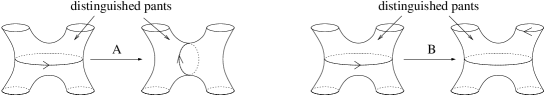
Figure 8: Moves in the Ptolemy groupoid

$\bullet$ The objects are the isotopy classes of asymptotically trivial rigid structures of ${\Sigma}_{0,\infty}$, with a distinguished oriented circle (among the circles of the rigid structure). The pair of pants bounded by the distinguished circle, which induces on the latter the opposite orientation, is called the distinguished pair of pants (see Figure 8).

$\bullet$ The morphisms are words in the moves $T,B,\Pi$ and $A$, defined as follows:

– The moves $T$ and $\Pi$ change a rigid structure as $t$ and $\pi$ do on Figures 4 and 5, respectively, where the represented supports must be viewed as the distinguished pairs of pants, the circles labeled 3 being the distinguished circles. Thus $T$ and $\Pi$ leave unchanged the pants decomposition subordinate to the rigid structure and the distinguished circle.

– The moves $B$ and $A$ change a rigid structure as $\beta$ and $\alpha$ do on Figures 6 and 7, respectively: on Figure 6, the represented supports must be viewed as the distinguished pairs of pants, the circles labeled 3 being the distinguished circles; on Figure 7, the circles which separate the adjacent pairs of pants are the distinguished circles, and the distinguished pants are labeled by P (see also Figure 8). Thus, the moves $B$ and $A$ leave unchanged the prerigid structure subordinate to the rigid structure.

$\bullet$ The relations between the moves are encoded in the assumption that for any rigid structure $r$, the group of morphisms ${\operatorname{Mor}}(r,r)$ must be trivial.

One denotes by ${\cal R}ig({\Sigma}_{0,\infty})$ the set of objects of ${{\cal D}_{0}^{s}}$. If $r$ and $r^{\prime}$ belong to ${\cal R}ig({\Sigma}_{0,\infty})$ and $W\in{\operatorname{Mor}}(r,r^{\prime})$ (or its inverse) is a move, one denotes its target $r^{\prime}$ by $W\cdot r$.

Remark 4.1.

The moves are only changing the rigid structure locally. In particular, the moves $B$ and $A$ do not rotate the whole picture. Rather in the first case, it just changes which circle is distinguished, and similarly for $A$.

Definition 4.2.

Let $M$ be the free group on $\{T,\Pi,A,B\}$. The group $M$ acts on ${\cal R}ig({\Sigma}_{0,\infty})$ via

$$M\times{\cal R}ig({\Sigma}_{0,\infty})\rightarrow{\cal R}ig({\Sigma}_{0,\infty})$$

$$\left(W=W_{1}\cdots W_{n},r\right)\mapsto W_{1}\cdots W_{n-1}W_{n}\cdot r$$

where $W_{i}^{\pm 1}\in\{T,\Pi,A,B\}$. Let $K$ be the kernel of the resulting morphism $M\rightarrow Aut({\cal R}ig({\Sigma}_{0,\infty}))$. The quotient $M/K$ is called the group of moves of the groupoid ${{\cal D}_{0}^{s}}$.

Proposition 4.2.

The group ${{\cal B}}$ and the group of moves $M/K$ are naturally anti-isomorphic. The anti-isomorphism is induced by $W=W_{n}\cdots W_{1}\in M\mapsto w=w_{1}\cdots w_{n}\in{{\cal B}}$, where $w_{i}^{\pm 1}=\alpha$ if $W_{i}^{\pm 1}=A$, $w_{i}^{\pm 1}=\beta$ if $W_{i}^{\pm 1}=B$, $w_{i}^{\pm 1}=\pi$ if $W_{i}^{\pm 1}=\Pi$, and $w_{i}^{\pm 1}=t$ if $W_{i}^{\pm 1}=T$. For all $W=W_{n}\cdots W_{1}\in M/K$, $W(r_{*})=w(r_{*})$, where $r_{*}$ is the canonical rigid structure.

Proof.

We first prove the last assertion. By definition of the generators $\alpha,\beta,\pi,t$, we have indeed $W_{1}(r_{*})=w_{1}(r_{*})$. But $W_{2}$ acts on $W_{1}(r_{*})$ as the conjugate of $w_{2}$ by $w_{1}$: $W_{2}(W_{1}(r_{*}))=(w_{1}w_{2}w_{1}^{-1})\cdot w_{1}(r_{*})=w_{1}(w_{2}(r_{*}))$. Inductively we check that $W(r_{*})=w(r_{*})$.

Since $M$ is free, the anti-morphism $W\in M\mapsto w\in{{\cal B}}$ is well-defined. It is surjective, since the image contains the generators of the group ${{\cal B}}$. Let $W=W_{1}\cdots W_{n}\in M$ be in the kernel of the anti-isomorphism i.e. $w=w_{n}\cdots w_{1}=1$ in ${{\cal B}}$. We prove that $W$ belongs to $K$.

For any rigid structure $r$, there exists some $w^{\prime}\in{{\cal B}}$ such that $r=w^{\prime}(r_{*})$. Choose $W^{\prime}\in M$ in the preimage of $w^{\prime}$. Then $W(r)=WW^{\prime}(r_{*})=w^{\prime}w(r_{*})=w^{\prime}(r_{*})=r$, so $W\in K$. Clearly, $K$ lies in the kernel of the anti-morphism, since if $w\in{{\cal B}}$ fixes pointwise a rigid structure, then it must be trivial. Hence $M/K$ is anti-isomorphic to ${{\cal B}}$. ∎

Remark 4.3.

We note from the proof above that $K$ coincides with the stabilizer of any rigid structure. Thus, for all $r,r^{\prime}$ in ${\cal R}ig({\Sigma}_{0,\infty})$, there exists a unique $W\in M/K$ such that $r^{\prime}=W\cdot r.$

4.2 ${{\cal D}_{0}^{s}}$ is a stabilization of ${\mathcal{D}}_{0}$, the duality groupoid in genus zero

The purpose of this subsection is to relate ${{\cal D}_{0}^{s}}$ with the the duality groupoid evoked in the Introduction. Its content will not be used in the sequel.

Definition 4.3.

The duality groupoid ${\mathcal{D}}$ considered in [9, 21] consists of the transformations of rigid structures. The duality groupoid of genus zero, ${\mathcal{D}}_{0}$, is the subgroupoid of ${\mathcal{D}}$ consisting of the transformations involving only genus zero surfaces:

$\bullet$ Its objects are pairs $(\Sigma,r_{\Sigma})$, where $\Sigma$ is a compact surface of genus zero, and $r_{\Sigma}$ is a rigid structure on $\Sigma$, which, in the sense of [9], consists of a decomposition of $\Sigma$ into pairs of pants, a collection of seams on the pairs of pants, a numbering of the pairs of pants, and for each pair of pants, a labeling by 1,2,3 of the boundary circles. They are defined up to isotopy.

$\bullet$ Its morphisms are changes of rigid structure.

There is a tensor structure $\otimes$ on ${\mathcal{D}}_{0}$, which corresponds to the connected sum along boundary components.

A finite presentation for ${\mathcal{D}}$ has been obtained in [9]. It is easy to check that the subset of generators $T_{1},B_{23},R,F$ and $P$ together with the relations provided in [9], which are involving only these generators, form a presentation for ${\mathcal{D}}_{0}$.

Proposition 4.4.

The duality groupoid of genus zero, ${\mathcal{D}}_{0}$, has the following presentation:

1. Generators: $T_{1},R,B_{23},F,P$ and their inverses.

2. Relations (Moore-Seiberg equations):
   1. at the level of a pair of pants:
    a) $T_{1}B_{23}=B_{23}T_{1}$, $T_{2}B_{23}=B_{23}T_{3}$,  $T_{3}B_{23}=B_{23}T_{2}$, where $T_{2}=R^{-1}T_{1}R$ and $T_{3}=RT_{1}R^{-1}$,
    b) $B_{23}^{2}=T_{1}T_{2}^{-1}T_{3}^{-1}$
    c) $R^{3}=1$
    d) $R=B_{23}RB_{23}R^{-1}T_{1}$
   2. relations defining inverses:
    a) $P^{(12)}F^{2}=1$
    b) $T_{3}^{-1}B_{23}^{-1}S^{2}=1$
   3. relations coming from “triangle singularities”:
    a) $P^{(13)}{R^{(2)}}^{2}F^{(12)}{R^{(2)}}^{2}F^{(23)}{R^{(2)}}^{2}F^{(12)}{R^{(2)}}^{2}F^{(23)}{R^{(2)}}^{2}F^{(12)}=1$
    b) $T_{3}^{(1)}FB_{23}^{(1)}FB_{23}^{(1)}FB_{23}^{(1)}=1$
   4. relations coming from the symmetric groups:
    a) $P^{2}=1$
    b) $P^{(23)}P^{(12)}P^{(23)}=P^{(12)}P^{(23)}P^{(12)}$
   

Remark 4.5.

We used the convention that superscripts tell us on which factors of the tensor product the move acts. Here the tensor structure is implicit. The pentagon relation 3.a) is corrected here since it was erroneously stated in [9] p.608 (see p.635) while the relation 1.d) was omitted.

The following proposition clarifies in which sense the stable groupoid in genus zero, ${{\cal D}_{0}^{s}}$, is indeed a stabilization of the duality groupoid ${\mathcal{D}}_{0}$.

View the group of moves $M/K$ of the groupoid ${{\cal D}_{0}^{s}}$ as the tautological groupoid (with a unique object, and $M/K$ as the set of morphisms).

Proposition 4.6.

There exists a surjective morphism of groupoids $s:{\mathcal{D}}_{0}\rightarrow M/K$.

Proof.

First, $s$ maps the objects of ${\mathcal{D}}_{0}$ on the unique object of $M/K$. Let $(\Sigma,r_{\Sigma})$ be an object of ${\mathcal{D}}_{0}$. The source and the target of any morphism of ${\mathcal{D}}_{0}$ may be represented by two rigid structures $r_{\Sigma}$ and $r_{\Sigma}^{\prime}$ on the same support $\Sigma$. So, let $\varphi:(\Sigma,r_{\Sigma})\rightarrow(\Sigma,r_{\Sigma}^{\prime})$ be such a morphism. One may identify $\Sigma$ with an admissible subsurface of ${\Sigma}_{0,\infty}$ (in a non-unique way). Let $r$ (resp. $r^{\prime}$) be the object of ${{\cal D}_{0}^{s}}$ with the following properties:

• it coincides ith the canonical rigid structure of ${\Sigma}_{0,\infty}$ outside $\Sigma$;

• it is induced by $r_{\Sigma}$ (resp. $r_{\Sigma}^{\prime}$) on $\Sigma$;

• its oriented circle is the labeled 1 circle of the labeled 1 pair of pants of $r_{\Sigma}$ (resp. $r_{\Sigma}^{\prime}$), viewed as the distinguished pair of pants of $r$ (resp. $r^{\prime}$), and oriented as explained in Definition 4.1.

There is a unique $W\in M/K$ such that $r^{\prime}=W\cdot r$ (see Remark 4.3). Moreover, $W$ does not depend on the choice of the representative $(\Sigma\subset{\Sigma}_{0,\infty},r_{\Sigma})$, but only on $\varphi$. One sets $s(\varphi)=W$ and this completes the definition of $s$. It is easy to check that $s(\varphi\psi)=s(\varphi)s(\psi)$.

If $\varphi$ is a morphism of type $T_{1}^{()},R^{()},B_{23}^{()}$ or $F^{()}$ (where the superscript tells us on which factors of the tensor product the move acts), then $s(\varphi)$ is conjugate (by some element $W\in M/K$ depending on the superscript) to a morphism of type $T,B,\Pi$ or $A^{-1}$ respectively. This easily implies the surjectivity of $s$. Notice that the image by $s$ of a move $P$ which transposes the numberings of two pairs of pants is a word in $A^{2}$ and $B$.∎

4.3 The stable duality groupoid ${{\cal D}_{0}^{s}}$ generalizes the universal Ptolemy groupoid

The universal Ptolemy groupoid ${\cal P}t$ appears in [23, 24, 15, 19]. We translate its definition to a language related to our framework:

Definition 4.4.

The universal Ptolemy groupoid ${\cal P}t$ is the full subgroupoid of ${{\cal D}_{0}^{s}}$ whose objects are the isotopy classes of asymptotically trivial pants decompositions (with distinguished oriented circles) which are compatible with the canonical prerigid structure. Hence the morphisms are the composites of the $A$ and $B$ moves (which suffice, since $A^{-1}=A^{3}$ and $B^{-1}=B^{2}$).

From Proposition 4.2, we may deduce that the group of moves of ${\cal P}t$ is anti-isomorphic to the subgroup of ${{\cal B}}$ generated by $\alpha$ and $\beta$: this is precisely the Ptolemy-Thompson group $T\subset V$, cf. Proposition 2.4. From the presentation of the group $T$, a presentation of the groupoid ${\cal P}t$ has been obtained in [19]: ${\cal P}t$ is presented by the generators $A$, $B$, and relations:

$$A^{4}=1,\;\;B^{3}=1,\;\;(AB)^{5}=1$$

$$[BAB,A^{2}BABA^{2}]=1,\;\;[BAB,A^{2}B^{2}A^{2}BABA^{2}BA^{2}]=1$$

This means that if a sequence of $A$ and $B$ moves starts and finishes at the same object, then the sequence is a product of conjugates of the sequences of the presentation. Equivalently, Ptolemy-Thompson’s group $T$ is presented by the generators $\alpha$, $\beta$, and the relations:

$${\alpha}^{4}=1,{\beta}^{3}=1,(\beta\alpha)^{5}=1,[\beta\alpha\beta,\alpha^{2}\beta\alpha\beta\alpha^{2}]=1,[\beta\alpha\beta,\alpha^{2}\beta^{2}\alpha^{2}\beta\alpha\beta\alpha^{2}\beta\alpha^{2}]=1$$

Definition 4.5.

Let $\operatorname{Gr}({\cal P}t)$ be the graph whose vertices are the objects of ${\cal P}t$, with edges corresponding to $A$ or $B$ moves.

Thus, $\operatorname{Gr}({\cal P}t)$ is a subcomplex of the classifying space of the category ${\cal P}t$, and is exactly the Cayley graph of Ptolemy-Thompson’s group $T$, generated by $\alpha$ and $\beta$. This assertion relies on the fact that in the Cayley graph of a group (with a chosen set of generators), there is an edge between two elements $g_{1}$ and $g_{2}$ if and only if $g_{1}^{-1}g_{2}$ is a generator of the group.

Remark 4.7.

The subgroup of $T$ generated by $\alpha^{2}$ and $\beta$ is isomorphic to $PSL(2,\mathbb{Z})$, viewed as the group of orientation preserving automorphisms of the planar tree ${\cal T}$ (see also Remark 2.1). Using the duality between ${\cal T}$ and the canonical pants decomposition, one deduces that, given two objects $r_{1}$ and $r_{2}$ of ${\cal P}t$ differing only by the position and the orientation of the distinguished circles, there exists a unique sequence of $B$ moves and squares of $A$ moves connecting $r_{1}$ to $r_{2}$.

5 The group ${{\cal B}}$ is finitely presented

The method we develop here follows the approach of Hatcher-Thurston in their proof that the mapping class groups of compact surfaces ([14]) are finitely presented. However, the Hatcher-Thurston complex of the (non-compact) surface ${\Sigma}_{0,\infty}$, even restricted to the asymptotically canonical pants decompositions, is too large for providing a finite presentation of ${\cal B}$. Instead, the ${\cal B}$-complex we construct (§5.3, Definition 5.5) will use Hatcher-Thurston complexes of compact holed-spheres with bounded levels only, together with simplicial complexes closely related to those used by K. Brown in the study of finiteness properties of the Thompson group $V$ (Brown-Stein complexes of bases, cf. [6]). By adding some cells to link both types of complexes and to kill some combinatorial loops, we shall obtain a simply connected ${\cal B}$-complex, with a finite number of cells modulo ${\cal B}$. By a standard theorem ([4]), it will follow that ${\cal B}$ is finitely presented.

As several complexes will appear throughout this section, we give below a road map for all of them. An arrow $``X\longrightarrow Y"$ means that the complex $X$ is introduced and studied for proving that the complex $Y$ is connected and simply connected.

\begin{picture}(0.0,0.0)\end{picture}

Nota bene: From now on, the topological objects associated to ${\Sigma}_{0,\infty}$, namely, the circles, the pants decompositions and the (pre)rigid structures, will be considered up to isotopy. This way, the group ${{\cal B}}$ acts on them.

5.1 Hatcher-Thurston complexes of the infinite surface

Definition 5.1.

Let ${\cal HT}({\Sigma}_{0,\infty})$ denote the Hatcher-Thurston complex of ${\Sigma}_{0,\infty}$:

1. The vertices are the asymptotically trivial pants decompositions of ${\Sigma}_{0,\infty}$.

2. The edges correspond to pairs of pants decompositions $(p,p^{\prime})$ which differ by a local A move, i.e. $p^{\prime}$ is obtained from $p$ by replacing one curve $\gamma$ in $p$ by a curve $\gamma^{\prime}$ that intersects $\gamma$ twice.

3. The 2-cells are introduced to fill in the cycles of moves of the following types: triangular cycles, square cycles (of disjointly supported A moves) and pentagonal cycles (cf. [14, 13]).

Remark 5.1.

A pants decomposition is codified by a Morse function on the surface. Then the A move is the elementary non-trivial change induced by a small isotopy among smooth functions which crosses once transversally the discriminant locus made of functions in Cerf’s stratification, and it is therefore a local change in this respect, too.

Remark 5.2.

We should mention that an $A$ move involves unoriented circles, unlike the $A$ move in the Ptolemy groupoid.

Remark 5.3.

A triangular (resp. pentagonal) 2-cell $\sigma$ is determined by a connected subsurface $\Sigma\subset{\Sigma}_{0,\infty}$ of level 4 (resp. 5), an asymptotically trivial pants decomposition $p_{\sigma}$ on ${\Sigma}_{0,\infty}\setminus\Sigma$, and a cycle of three (resp. five) A moves inside $\Sigma$ (cf. Figure 9).

A square 2-cell, generically denoted $(DC)$, is determined by two disjoint or adjacent connected subsurfaces $\Sigma$ and $\Sigma^{\prime}$ of level 4, an asymptotically trivial pants decomposition $p_{(DC)}$ on ${\Sigma}_{0,\infty}\setminus(\Sigma\cup\Sigma^{\prime})$, and two A moves, supported in $\Sigma$ and $\Sigma^{\prime}$, respectively. One defines an integer associated to $(DC)$, called the distance $d_{(DC)}$: this is the minimal integer $r\geq 0$ such that there exists pairs of pants $P_{1},\ldots,P_{r}$ belonging to $p_{(DC)}$, with $P_{1}$ adjacent to $\Sigma$, $P_{r}$ adjacent to $\Sigma^{\prime}$, and $P_{i}$ adjacent to $P_{i+1}$, for all $i=1,\ldots,r-1$.

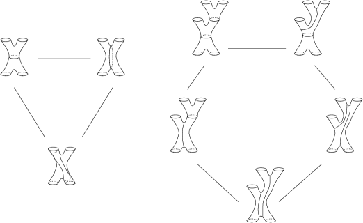
Figure 9: Triangular cycle and pentagonal cycle in ${\cal HT}({\Sigma}_{0,\infty})$

Proposition 5.4.

The complex ${\cal HT}({\Sigma}_{0,\infty})$ is connected and simply connected. The group ${{\cal B}}$ acts cellularly on it, with one orbit of 0-cells, one orbit of 1-cells, one orbit of triangular 2-cells, one orbit of pentagonal 2-cells, but countably many orbits of square 2-cells. Two square 2-cells $(DC)$ and $(DC^{\prime})$ are in the same orbit if, and only if, $d_{(DC)}=d_{(DC^{\prime})}$.

Proof.

The first assertion results from [14, 13], by describing the complex as an inductive limit of the Hatcher-Thurston complexes ${\cal HT}(S)$ of the admissible supports $S\subset{{\Sigma}_{0,\infty}}$, with respect to the various inclusions $S\subset S^{\prime}$. Equivalently, if one wants to connect $p$ to $p^{\prime}$, it is enough to do so in the pants complex for some surface “containing” both, and similarly for the simple connectedness.

That ${{\cal B}}$ acts transitively on the set of 0-cells and on the set of 1-cells is obvious. Consider next two triangular 2-cells $\sigma_{1}$ and $\sigma_{2}$. Let $\Sigma_{i}$ ($i=1,2$) be the subsurface of level 4 of ${\Sigma}_{0,\infty}$ which supports the three A moves involved in $\sigma_{i}$ ($i=1,2$) and $p_{\sigma_{i}}$ ($i=1,2$) be the pants decomposition outside $\Sigma_{i}$ (cf. Remark 5.3). Denote by $\overline{\sigma_{i}}$ the triangular 2-cell corresponding to $\sigma_{i}$, viewed in ${\cal HT}(\Sigma_{i})$. Since ${\cal M}(0,4)$ acts transitively on the 2-cells of ${\cal HT}(\Sigma_{0,4})$, one deduces that there exists a homeomorphism from $\Sigma_{1}$ to $\Sigma_{2}$ mapping $\overline{\sigma_{1}}$ onto $\overline{\sigma_{2}}$. The pants decomposition $p_{\sigma_{1}}$ and $p_{\sigma_{1}}$ being asymptotically trivial, one can extend $h$ to an asymptotically rigid homeomorphism of ${\Sigma}_{0,\infty}$ which maps $p_{\sigma_{1}}$ onto $p_{\sigma_{2}}$. The resulting mapping class belongs to ${{\cal B}}$, and maps the cell $\sigma_{1}$ onto $\sigma_{2}$.

Using the transitivity of the action of ${\cal M}(0,5)$ on the pentagonal 2-cells of $\Sigma_{0,5}$, one proves similarly that there exists a unique orbit of pentagonal 2-cells in ${\cal HT}({\Sigma}_{0,\infty})$.

Finally, one proves by similar arguments that two square 2-cells $(DC)$ and $(DC^{\prime})$ are equivalent modulo ${{\cal B}}$ if and only if $d_{(DC)}=d_{(DC^{\prime})}$. ∎

Definition 5.2.

(Reduced Hatcher-Thurston complex)
Let ${\cal HT}_{red}({\Sigma}_{0,\infty})$ be the subcomplex of ${\cal HT}({\Sigma}_{0,\infty})$ whose vertices, edges, triangular, and pentagonal 2-cells are those of ${\cal HT}({\Sigma}_{0,\infty})$, but whose square 2-cells are of two types:

1. Square $(DC1)$, associated with two commuting moves on two 4-holed spheres adjacent along a common boundary circle (hence $d_{(DC1)}=0$), cf. Figure 10;

2. Square $(DC2)$, associated with two commuting moves on two 4-holed spheres separated by a pants surface (hence $d_{(DC2)}=0$), cf. Figure 10.

\begin{picture}(0.0,0.0)\end{picture}

Figure 10: Cells (DC1) and (DC2)

The next proposition plays a key role in the proof of Theorem 1.1. It relies on the existence of a cellular map $\nu:\operatorname{Gr}({\cal P}t)\rightarrow{\cal HT}({\Sigma}_{0,\infty})$.

Proposition 5.5.

The reduced Hatcher-Thurston complex ${\cal HT}_{red}({\Sigma}_{0,\infty})$ is connected and simply connected. The group ${{\cal B}}$ acts cellularly on it, with one orbit of 0-cells, one orbit of 1-cells, one orbit of triangular 2-cells, one orbit of pentagonal 2-cells, and two orbits of square 2-cells.

Proof.

It suffices to prove that each square cycle $(DC)$ corresponding to two commuting moves which are supported on arbitrarily far disjoint 4-holed spheres is a product of conjugates of square cycles of types $(DC1)$ and $(DC2)$ and of pentagonal cycles. We use the Ptolemy groupoid. Let $\operatorname{Gr}({\cal P}t)$ be the graph introduced in Definition 4.5. There is an obvious forgetful cellular map

$$\nu:\operatorname{Gr}({\cal P}t)\rightarrow{\cal HT}({\Sigma}_{0,\infty})$$

defined on the set of vertices by forgetting the orientation of the distinguished circle and the fact that it is distinguished. The cycles of $\operatorname{Gr}({\cal P}t)$ corresponding to the first three relations of ${\cal P}t$ project by $\nu$ onto cycles of ${\cal HT}({\Sigma}_{0,\infty})$. The projection by $\nu$ of the cycle $C_{A^{4}}$ corresponding to $A^{4}$ is a degenerate cycle of the form $ee^{-1}ee^{-1}$, where $e$ is an oriented edge and $e^{-1}$ the edge with the opposite orientation; $\nu(C_{B^{3}})$ is a 0-cell and $\nu(C_{(AB)^{5}})$ is a pentagonal cycle. It is elementary to check that $\nu(C_{[BAB,A^{2}BABA^{2}]})$ is a square cycle of type $(DC1)$, and $\nu(C_{[BAB,A^{2}BA^{2}BABA^{2}B^{2}A^{2}]})$ a square cycle of type $(DC2)$.

Now let $(DC)$ be an arbitrary square cycle of ${\cal HT}({\Sigma}_{0,\infty})$. We can find an asymptotically trivial prerigid structure $r$ such that the four vertices of $(DC)$, that is, the four pants decompositions, are all compatible with $r$. At the price of replacing $(DC)$ by an equivalent (hence homeomorphic) cycle modulo ${{\cal B}}$, we may suppose that $r$ is the canonical prerigid structure. It follows that we can find a “lift” $\widetilde{(DC)}$ of $(DC)$ in $\operatorname{Gr}({\cal P}t)$ as follows. We first lift the 4 edges $e_{1},\ldots,e_{4}$ of $(DC)$ to 4 edges $\widetilde{e_{1}},\ldots,\widetilde{e_{4}}$, corresponding to $A$ moves in ${\cal P}t$. Since the terminal vertex $t(\widetilde{e_{i}})$ of $\widetilde{e_{i}}$ and the origin $o(\widetilde{e_{i+1}})$ of $\widetilde{e_{i+1}}$ (for $i=1,\ldots,4$ mod 4) are pants decompositions which differ by the positions of the distinguished circle, we must (and can) find an edge-path $\gamma_{i}$ in $\operatorname{Gr}({\cal P}t)$ joining $t(\widetilde{e_{i}})$ to $o(\widetilde{e_{i+1}})$. By Remark 4.7, $\gamma_{i}$ is a composite of $B$ moves and squares of $A$ moves. Let now $\widetilde{(DC)}$ be the cycle $\widetilde{e_{1}}\gamma_{1}\widetilde{e_{2}}\gamma_{2}\widetilde{e_{3}}\gamma_{3}\widetilde{e_{4}}\gamma_{4}$. Since $\nu(B)$ is a point and $\nu(A^{2})$ is homotopic to a point, $\nu(\widetilde{(DC)})$ is homotopically equivalent to $(DC)$. But the cycle $\widetilde{(DC)}$ can be expressed as a product of conjugates of cycles of the presentation of ${\cal P}t$. We then project this product of cycles onto ${\cal HT}({\Sigma}_{0,\infty})$, and obtain $\nu(\widetilde{(DC)})$, expressed as a product of conjugates of cycles of the subcomplex ${\cal HT}_{red}({\Sigma}_{0,\infty})$ (namely, pentagons, squares $(DC1)$ and $(DC2)$, and degenerate cycles of the form $\nu(A^{2})$). Therefore, the cycle $(DC)$ is homotopically trivial in ${\cal HT}_{red}({\Sigma}_{0,\infty})$.

The last assertion of the proposition is a direct consequence of Proposition 5.4. ∎

5.2 An auxiliary pants decomposition complex

Our main object will be a ${\cal B}$-complex ${\cal DP}({\Sigma}_{0,\infty})$, which is connected, simply connected and finite modulo ${\cal B}$. In order to prove its simple connectivity, we introduce an auxiliary complex $\widetilde{\cal DP}({\Sigma}_{0,\infty})$ containing ${\cal DP}({\Sigma}_{0,\infty})$, and prove that it is simply connected. By studying the inclusion ${\cal DP}({\Sigma}_{0,\infty})\subset\widetilde{\cal DP}({\Sigma}_{0,\infty})$, we finally prove the same property for ${\cal DP}({\Sigma}_{0,\infty})$.

Definition 5.3 (Complex $\widetilde{\cal DP}({\Sigma}_{0,\infty})$).

The complex $\widetilde{\cal DP}({\Sigma}_{0,\infty})$ is a two-dimensional cellular complex whose vertices are triples $(p,S,r)$, where:

• $p$ is an asymptotically trivial pants decomposition of ${\Sigma}_{0,\infty}$,

• $S$ is a surface of level $l\in\{3,\ldots,7\}$, compatible with $p$ (or p-compatible), that is, a connected compact subsurface of ${\Sigma}_{0,\infty}$ of level $l$ bounded by circles of $p$, and endowed with the pants decomposition induced by $p$ (but devoid of its seams), and

• $r$ is a rigid structure on ${\Sigma}_{0,\infty}\setminus S$, to which $p$ is subordinate outside $S$.

One says that the level of $(p,S,r)$ is $l$ (see Figure 11), and that $S$ is its support.

Figure 11: A vertex $(p,S,r)$ of level 4 of $\widetilde{\cal DP}({\Sigma}_{0,\infty})$

There are 1-cells associated with moves of three kinds:

1. $A$ moves: they are defined as in the Hatcher-Thurston complexes, but we restrict to those which preserve the support $S$ and the rigid structure $r$ of a vertex $(p,S,r)$, and change the pants decomposition $p$ inside $S$.

2. Propagation moves $P$: a $P$ move on $(p,S,r)$ consists of choosing (finitely many) pairs of pants of $p$ inside ${\Sigma}_{0,\infty}\setminus S$, all adjacent to $S$, and erasing their seams. This changes $(p,S,r)$ into $(p,S^{\prime},r^{\prime})$, where $S^{\prime}\supset S$, and $r^{\prime}$ coincides with $r$ on ${\Sigma}_{0,\infty}\setminus S^{\prime}$. One also says that $(p,S,r)$ results from $(p,S^{\prime},r^{\prime})$ by a $P^{-1}$ move.

3. Braiding moves $Br$: a braiding move on $(p,S,r)$, supported on a pair of pants ${\cal P}\subset{\Sigma}_{0,\infty}\setminus S$ belonging to $p$, consists of changing only the rigid structure $r$ on ${\cal P}$. The terminology is justified by the fact that a braiding move may be realized by an element of ${\cal M}({\cal P})$.

The 2-cells are introduced to fill in the following cycles of moves:

1. Triangles (see Figure 16), pentagons, squares of commutativity of $A$ moves of type $(DC1)$ and $(DC2)$ (see Figure 10, forgetting about the orientation of the circles, or Figures 18 and 19): they all involve vertices with the same support, of level $4,5,6$ or $7$, respectively.

2. Triangles of $P$ moves: suppose that the action of a $P$ move on $(p,S,r)$ yields $(p,S^{\prime},r^{\prime})$ and consider another $P$ move on $(p,S^{\prime},r^{\prime})$ which is erasing seams of pairs of pants adjacent to $S$, and hence to $S^{\prime}$. Then the composition of the two $P$ moves is again a $P$ move, and there results a triangle $PP=P$ (see Figure 12).

3. Squares of commutativity of $P$ moves with $A$ moves (see Figure 12).

   

   Figure 12: $2$-cells $PP=P$ and $PA=AP$

4. 1. Triangles of $Br$ moves: suppose that the action of a $Br$ move on $(p,S,r)$, supported on a pair of pants ${\cal P}\subset{\Sigma}_{0,\infty}\setminus S$ belonging to $p$, yields $(p,S^{\prime},r^{\prime})$, and consider another $Br$ move on $(p,S^{\prime},r^{\prime})$ supported on the same ${\cal P}$. Then the composition of the two $Br$ moves is again a $Br$ move, and there results a triangle $Br\,Br=Br$.

   2. Squares of commutativity of $Br$ moves supported on two distinct pairs of pants: let $(p,S,r)$ be a vertex, ${\cal P}$ and ${\cal Q}$ be two pairs of pants of ${\Sigma}_{0,\infty}\setminus S$, belonging to $p$. If $Br_{\cal P}$ and $Br_{\cal Q}$ denote braiding moves supported on ${\cal P}$ and ${\cal Q}$, respectively, then the actions of $Br_{\cal P}Br_{\cal Q}$ (i.e. $Br_{\cal Q}$ followed by $Br_{\cal P}$) and $Br_{\cal Q}Br_{\cal P}$ on $(p,S,r)$ yield the same vertex.

5. Squares of commutativity of $Br$ moves with $A$ moves, and squares of commutativity of $Br$ moves with $P$ moves (see Figure 13).

6. Triangles $P^{-1}P=Br$ (see Figure 13): a $P$ move erasing the rigid structure on a single pair of pants followed by a $P^{-1}$ move introducing a new rigid structure on the same pair of pants has the same effect as a $Br$ move. (Notice that these may be seen as degenerate squares of commutativity of $P$ moves with $Br$ moves).

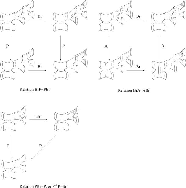
Figure 13: $2$-cells involving $Br$ moves

Proposition 5.6.

The complex $\widetilde{\cal DP}({\Sigma}_{0,\infty})$ is connected and simply connected.

The proof will use twice the following lemma of algebraic topology from ([2], prop. 6.2, see also a variant of it in [9]):

Lemma 5.7.

Let ${\cal M}$ and ${\cal C}$ be two $CW$-complexes of dimension $2$, with oriented edges, and $f:{\cal M}^{(1)}\rightarrow{\cal C}^{(1)}$ be a cellular map between their 1-skeletons, surjective on $0$-cells and $1$-cells. Suppose that:

1. ${\cal C}$ is connected and simply connected;

2. For each vertex $c$ of ${\cal C}$, $f^{-1}(c)$ is connected and simply connected;

3. Let $c_{1}\stackrel{{\scriptstyle e}}{{\longrightarrow}}c_{2}$ be an oriented edge of ${\cal C}$, and let $m_{1}^{\prime}\stackrel{{\scriptstyle e^{\prime}}}{{\longrightarrow}}m_{2}^{\prime}$ and $m_{1}"\stackrel{{\scriptstyle e"}}{{\longrightarrow}}m_{2}"$ be two lifts in ${\cal M}$. Then we can find two paths $m_{1}^{\prime}\stackrel{{\scriptstyle p_{1}}}{{\longrightarrow}}m_{1}^{\prime\prime}$ in $f^{-1}(c_{1})$ and $m_{2}^{\prime}\stackrel{{\scriptstyle p_{2}}}{{\longrightarrow}}m_{2}^{\prime\prime}$ in $f^{-1}(c_{2})$ such that the loop

   \begin{picture}(0.0,0.0)\end{picture}

   is contractible in ${\cal M}$;

4. For any $2$-cell $X$ of ${\cal C}$, its boundary $\partial X$ can be lifted to a contractible loop of ${\cal M}$.

Then ${\cal M}$ is connected and simply connected.

Proof of Proposition 5.6. Let $F:\widetilde{\cal DP}({\Sigma}_{0,\infty})\rightarrow{\cal HT}_{red}({\Sigma}_{0,\infty})$ be the cellular map induced by the map $(p,S,r)\mapsto p$ on the set of vertices, which forgets about the rigid structure (and support $S$). The restriction of $F$ to the 1-skeletons is indeed surjective. We have proved also that ${\cal HT}_{red}({{\Sigma}_{0,\infty}})$ is connected and simply connected. The squares of commutativity of $A$ moves with $P$ moves and $Br$ moves insure condition 3. Condition 4 is satisfied by using 2-cells of type 1. It remains to check condition 2.

Let $p$ be a $0$-cell of ${\cal HT}_{red}({\Sigma}_{0,\infty})$, i.e. an asymptotically trivial pants decomposition of ${\Sigma}_{0,\infty}$. Then $F^{-1}(p)$ is the subcomplex of $\widetilde{\cal DP}({\Sigma}_{0,\infty})$ with vertices $(p,S,r)$ and edges corresponding to $P$ moves and $Br$ moves.

To study the connectivity of $F^{-1}(p)$, we introduce a new map which forgets about the pants decomposition and the rigid structure:

$$G:{F^{-1}(p)}\rightarrow sk_{2}({\cal BS}_{3,7}(p))$$

where $sk_{2}(X)$ denotes the 2-skeleton of the complex $X$ and ${\cal BS}_{3,7}(p)$ is a subcomplex of a simplicial complex ${\cal BS}(p)$ that we now define:

Definition 5.4 (A variant of Brown-Stein’s complex of bases, cf. [6]).

Let $S$ and $S^{\prime}$ be two surfaces compatible with $p$ (see Definition 5.3). One says that $S^{\prime}$ is a simple expansion of $S$ if $S^{\prime}$ is the union of $S$ with a pair of pants of $p$ adjacent to $S$ (so that $l(S^{\prime})=l(S)+1$). Further $S^{\prime}$ is an expansion of $S$ if it is obtained from $S$ by a sequence of simple expansions.

One denotes by $S\leq S^{\prime}$ when $S^{\prime}$ is an expansion of $S$: this endows the set of $p$-compatible surfaces with a poset structure. One denotes by ${\cal B}(p)$ the associated simplicial complex.

One says that $S^{\prime}$ is an elementary expansion of $S$ if $S^{\prime}$ is the union of $S$ with (finitely many) pairs of pants of $p$ adjacent to $S$.

One defines the elementary $n$-simplices as the $(n+1)$-tuples $(U_{0},\ldots,U_{n})$ with $U_{0}\leq\ldots\leq U_{n}$ and $U_{n}$ an elementary expansion of $U_{0}$ (so that each $U_{j}$ is an elementary expansion of $U_{i}$, $0\leq i\leq j\leq n$). The set of all elementary simplices forms a simplicial subcomplex ${\cal BS}(p)$ of ${\cal B}(p)$.

Remark 5.8.

The complexes ${\cal BS}(p)\subset{\cal B}(p)$ are closely related to simplicial complexes introduced by K. Brown and M. Stein ([6]) in the study of Thompson’s group $V$. Since the complex ${\cal B}(p)$ is associated to a direct poset, it is contractible. It happens that ${\cal BS}(p)$ is also contractible: this can be proved by repeating step by step M. Stein’s proof of the contractibility of the analogous bases complex of elementary simplices ([6]).

Denote by ${\cal BS}_{3,n}(p)$, $n\geq 3$, the full subcomplex of ${\cal BS}(p)$ whose vertices are the $p$-compatible surfaces $S\subset p$ of level in $\{3,\ldots,n\}$.

Lemma 5.9.

For all $n\geq 5$, ${\cal BS}_{3,n}(p)$ is contractible.

Proof.

Since ${\cal BS}(p)$ is the ascending union of the subcomplexes ${\cal BS}_{3,n}(p)$, $n\geq 5$, it suffices to prove that each inclusion ${\cal BS}_{3,n}(p)\subset{\cal BS}_{3,n+1}(p)$ is a homotopy equivalence. We pass from ${\cal BS}_{3,n}(p)$ to ${\cal BS}_{3,n+1}(p)$ by considering each $p$-compatible surface $S$ of level $n+1$, and attaching to ${\cal BS}_{3,n}(p)$ a cone on $S$ over the link of $S$. But the link, which is contained in ${\cal BS}_{3,n}(p)$, is contractible, since it can be contracted on the minimal vertex $S^{\prime}$, obtained from $S$ by removing all its outermost pairs of pants. Note that this is possible because $n\geq 5$. ∎

In particular, the $2$-skeletons $sk_{2}({\cal BS}_{3,n}(p))$, $n\geq 5$, are connected and simply connected.

The forgetful map $G:F^{-1}(p)\rightarrow sk_{2}({\cal BS}_{3,7}(p))$ is induced on the set of vertices by the map $(p,S,r)\mapsto S$. It maps a $P$ move onto an edge of ${\cal BS}_{3,7}(p)$, and a 2-cell of type $PP=P$ onto a 2-simplex of ${\cal BS}_{3,7}(p)$. It follows from the above lemma that condition 1 of Lemma 5.7 is satisfied. The preimage of a 0-cell is contractible in the full complex, since the combinatorial cycles in this preimage can be filled in by 2-cells of types 4a and 4b of Definition 5.3. Condition 4 is satisfied, since $G$ is surjective on the set of $2$-cells. Finally the squares of commutativity of $P$ moves with $Br$ moves together with the triangles $P^{-1}P=Br$ imply condition 3. This completes the proof that $F^{-1}(p)$ is connected and simply connected, and thus completes the proof of Proposition 5.6. $\;\;\;\square$

5.3 The complex ${\cal DP}({\Sigma}_{0,\infty})$ and the main theorem for ${{\cal B}}$

Definition 5.5.

Let ${\cal DP}({\Sigma}_{0,\infty})$ be the subcomplex of $\widetilde{\cal DP}({\Sigma}_{0,\infty})$ obtained from the latter by eliminating all edges and $2$-cells involving $Br$ moves. In other words, ${\cal DP}({\Sigma}_{0,\infty})$ is the cellular complex whose vertices are triples $(p,S,r)$ as in Definition 5.3, with edges corresponding to $A$ moves and $P$ moves, and three distinct families of $2$-cells:

1. Hatcher-Thurston-type cells: triangles, pentagons, and squares $(DC1)$ and $(DC2)$;

2. Brown-Stein-type cells ($2$-simplices): $PP=P$;

3. Squares of commutativity $PA=AP$.

Notice that the cells of third kind are connecting Hatcher-Thurston-type cells to Brown-Stein-type cells.

Theorem 5.10.

The complex ${\cal DP}({\Sigma}_{0,\infty})$ is a connected and simply connected ${\cal B}$-complex, with finite quotient ${\cal DP}({\Sigma}_{0,\infty})/{\cal B}$. In particular, ${\cal B}$ is a finitely presented group.

Proof.

By adapting the arguments of the proof of Proposition 5.4, one proves that ${\cal DP}({\Sigma}_{0,\infty})$ has a finite number of cells modulo ${{\cal B}}$. The last assertion is therefore a direct application of K. Brown’s theorem on presentations for groups acting on simply connected $CW$-complexes, in the case of finitely presented vertex stabilizers and finitely generated edge stabilizers (which is the case here, cf. the next subsection). To prove the first assertion, we show that $\widetilde{\cal DP}({\Sigma}_{0,\infty})$ is obtained from ${\cal DP}({\Sigma}_{0,\infty})$ by attaching countably many $2$-spheres at each $0$-cell of ${\cal DP}({\Sigma}_{0,\infty})$. Our strategy is to examine below cells of type 4a in step 1, 4b in step 2, and 5-6 in step 3.

1. Consider first a $2$-cell $\omega_{a}$ bounded by a triangle of $Br$ moves, all supported on the same pair of pants ${\cal P}\subset{\Sigma}_{0,\infty}\setminus S$, with vertices $(p,S,r_{i})$, $i=1,2$ and 3, cf. Definition 5.3, 4a). The rigid structures $r_{i}$ only differ from each other on the pants ${\cal P}$. We may find a sequence of $P$ moves and $P^{-1}$ moves $P_{1}^{\pm 1}P_{2}^{\pm 1}\cdots P_{n}^{\pm 1}$ translating $S$ to another $p$-compatible surface $\tilde{S}$ containing ${\cal P}$, since $l(S)\geq l({\cal P})$. By using the squares of commutativity $P_{i}Br=BrP_{i}$ and the degenerate squares (or triangles) $P_{i}Br=P_{i}$, the initial triangle of $Br$ moves is replaced, $P^{\pm 1}$ move by $P^{\pm 1}$ move, by a conjugate triangle. The edge-paths of $P^{\pm 1}$ moves starting from the 3 different vertices $(p,S,r_{i})$ end at the same vertex $(p,\tilde{S},\tilde{r})$ (since $\tilde{S}$ contains the pants ${\cal P}$ on which the 3 rigid structures differ from each other). Thus, adding the $2$-cell $\omega_{a}$ to ${\cal DP}({\Sigma}_{0,\infty})$ is homotopically equivalent to attaching $2$-spheres at the vertex $(p,\tilde{S},\tilde{r})$.

2. Consider now a $2$-cell $\omega_{b}$ bounded by a square cycle of commutativity between two $Br$ moves supported on two distinct pairs of pants ${\cal P}$ and ${\cal P}^{\prime}$ (subordinate to the same $(p,S)$, cf. Definition 5.3, 4b)). The four vertices of the square correspond to pairs $(p,S,r_{i})$, $i=1,\ldots,4$, the pants decomposition $p$ being fixed as well as the support $S$, but the rigid structure $r_{i}$ differing from each other only on ${\cal P}$ and/or ${\cal P}^{\prime}$.

   Let $\Sigma_{{\cal PP}^{\prime}}$ be the minimal compact subsurface, compatible with $p$, connecting ${\cal P}$ to ${\cal P}^{\prime}$ (see Figure 14). By changing the pants decomposition $p$ inside $\Sigma_{{\cal PP}^{\prime}}$, we may find a pants decomposition $\tilde{p}$ such that ${\cal P}$ and ${\cal P}^{\prime}$ (which are still compatible with $\tilde{p}$) belong to a same surface $\tilde{S}$ of level at most 5, compatible with $\tilde{p}$ (see Figure 14).

   \begin{picture}(0.0,0.0)\end{picture}

   Figure 14: From $p$ to $\tilde{p}$

   Consider next the pants decompositions $p$ and $\tilde{p}$ in the Hatcher-Thurston complex of ${\Sigma}_{0,\infty}$. Since they only differ on ${\Sigma}_{{\cal PP}^{\prime}}$, the connectedness of the Hatcher-Thurston complex of ${\Sigma}_{{\cal PP}^{\prime}}$ enables us to find a sequence of $A$ moves $A_{1}A_{2}\cdots A_{n}$ connecting $p$ to $\tilde{p}$, and all supported in ${\Sigma}_{{\cal PP}^{\prime}}$. Now an $A$ move in ${\cal DP}({\Sigma}_{0,\infty})$ is possible only inside a support devoid of its seams. Therefore, we lift to ${\cal DP}({\Sigma}_{0,\infty})$ the sequence of moves $A_{1}A_{2}\cdots A_{n}$ into four edge paths starting from each $(p,S,r_{i})$, by inserting an adequate number of $P^{\pm 1}$ moves between the $A$ moves of the sequence $A_{1}A_{2}\cdots A_{n}$. The four edge paths end at a same vertex $(\tilde{p},\tilde{S},\tilde{r})$, and we conclude as in 1), using the squares $PBr=BrP$ and $ABr=BrA$.

3. Notice finally that each square $PBr=BrP$, $ABr=BrA$, belongs to a 2-sphere obtained in 1) or 2), and thus can be eliminated with the cells $\omega_{a}$ and $\omega_{b}$.

∎

6 A finite presentation for the group ${\cal B}$

6.1 Reduction of ${\cal DP}({\Sigma}_{0,\infty})$ to the complex ${\cal DP}^{+}_{5}({\Sigma}_{0,\infty})$

Consider the full subcomplex ${\cal DP}_{5}({\Sigma}_{0,\infty})$ whose levels of vertices belong to $\{3,4,5\}$. The boundaries of the $2$-cells of type $(DC1)$ and $(DC2)$ in ${\cal DP}_{5}({\Sigma}_{0,\infty})$ do not belong to ${\cal DP}_{5}({\Sigma}_{0,\infty})$, but are homotopic to cycles ${\cal C}_{1}$ and ${\cal C}_{2}$ of ${\cal DP}_{5}({\Sigma}_{0,\infty})$, respectively (cf. Figure 18 and Figure 19). Indeed, the “area” between the boundary of $(DC1)$ and the cycle ${\cal C}_{1}$ (resp. $(DC2)$ and the cycle ${\cal C}_{2}$) may be filled in by squares $PA=AP$ and simplices $PP=P$.

Note that the cycles ${\cal C}_{1}$ (resp. ${\cal C}_{2}$), which are of length $12$ (resp. of length $20$), are all equivalent modulo ${\cal B}$.

Definition 6.1.

Let ${\cal DP}^{+}_{5}({\Sigma}_{0,\infty})$ be the complex obtained from ${\cal DP}_{5}({\Sigma}_{0,\infty})$ by adding $2$-cells to fill in the cycles of types ${\cal C}_{1}$ and ${\cal C}_{2}$.

Proposition 6.1.

The ${\cal B}$-complex ${\cal DP}^{+}_{5}({\Sigma}_{0,\infty})$ is connected and simply connected, and finite modulo ${\cal B}$.

Proof.

From Figures 18 and 19, each cell of type (DC1) or (DC2) gives rise to countably many “big squares”, which are therefore homeomorphic to $2$-cells, attached to ${\cal DP}^{+}_{5}({\Sigma}_{0,\infty})$ along contractible cycles ${\cal C}_{1}$ or ${\cal C}_{2}$. They are made up of squares (DC1) or (DC2), squares $PA=AP$, and simplices $PP=P$.

Similarly, consider the other $2$-cells of the closure of ${\cal DP}({\Sigma}_{0,\infty})\setminus{\cal DP}_{5}({\Sigma}_{0,\infty})$: the Hatcher-Thurston triangles and pentagons (on supports of levels $6$ or $7$) are attached along similar triangular and pentagonal cycles of ${\cal DP}_{5}({\Sigma}_{0,\infty})$, via squares $PA=AP$; the simplices $PP=P$ also are attached along contractible cycles via other simplices $PP=P$.

All squares $PA=AP$ and simplices $PP=P$ have been used in proceeding to the above attachments. It follows that the closure of ${\cal DP}({\Sigma}_{0,\infty})\setminus{\cal DP}_{5}({\Sigma}_{0,\infty})$ is homeomorphic to a union of closed $2$-cells, all attached to ${\cal DP}^{+}_{5}({\Sigma}_{0,\infty})$ along contractible cycles. ∎

Set ${\cal F}$ of essential $2$-cells: Notice first that the triangles of ${\cal DP}^{+}_{5}({\Sigma}_{0,\infty})$ on supports of level $5$ are conjugate, via $P$-edges, to triangles on supports of level $4$. Further, replace the simplices $PP=P$ by squares $PP=PP$ involving two adjacent simplices (cf. Figure 15).

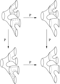
Figure 15: Square $PP=PP$

This does not affect the homeomorphism type of ${\cal DP}^{+}_{5}({\Sigma}_{0,\infty})$, and by abuse of notation, we still denote the modified complex by ${\cal DP}^{+}_{5}({\Sigma}_{0,\infty})$. It follows that there are 6 essential 2-cells in ${\cal DP}^{+}_{5}({\Sigma}_{0,\infty})$ modulo ${\cal B}$ (cf. Figures 16, 17, 18 and 19).

\begin{picture}(0.0,0.0)\end{picture}

Figure 16: Relations associated to the pentagon and the triangle

\begin{picture}(0.0,0.0)\end{picture}

Figure 17: Relations associated to the cells $PA=AP$ and $PP=PP$

\begin{picture}(0.0,0.0)\end{picture}

Figure 18: Relation associated to the cell $(DC1)$

\begin{picture}(0.0,0.0)\end{picture}

Figure 19: Relation associated to the cell $(DC2)$

6.2 The method: K. Brown’s theorem for groups acting on simply connected complexes

Let us denote by $Tr$ a tree of representatives of ${\cal DP}_{5}^{+}({\Sigma}_{0,\infty})$ modulo ${\cal B}$, with set of vertices $Vert=\{v_{1},v_{2},v_{3}\}$, linked by $P$ edges $e_{1}$ and $e_{2}$ as indicated in Figure 20. We assume that all the representatives are subordinate to the canonical rigid structure. We have only displayed the supports of the vertices, so that one has to imagine the canonical rigid structure outside each support.

\begin{picture}(0.0,0.0)\end{picture}

Figure 20: Tree $Tr$ and set of edges $E^{+}$

Each edge of ${\cal DP}_{5}^{+}({\Sigma}_{0,\infty})$ is equivalent modulo ${\cal B}$ to an edge with origin in $Tr$. There are exactly two such edges (modulo ${{\cal B}}$) which do not belong to $Tr$:

• the edge $e^{-}$: $v_{2}\stackrel{{\scriptstyle A}}{{\longrightarrow}}\alpha(v_{2})$, and

• the edge $e^{+}$: $v_{3}\stackrel{{\scriptstyle A}}{{\longrightarrow}}g(v_{3})$, where $g$ rotates the boundary components of the support of $v_{3}$ as indicated in Figure 21.

\begin{picture}(0.0,0.0)\end{picture}

Figure 21: Homeomorphism $g$

The orientation of the first edge $e^{-}$ can be inverted by the action of the group ${{\cal B}}$. We denote by $\sigma^{-}$ the cell underlying the oriented edge $e^{-}$.

Let $E^{+}$ be the set of edges of $Tr$ plus the edge $e^{+}$, whose orientation cannot be inverted by ${{\cal B}}$.

If $e$ is an edge, denote by $o(e)$ its initial vertex, and by $t(e)$ its terminal vertex. For each $e\in E^{+}$, denote by $w_{e}$ the unique vertex of $Tr$ equivalent to $t(e)$ modulo ${\cal B}$, and choose $g_{e}\in{\cal B}$ such that $t(e)=g_{e}\cdot w_{e}$: for instance $g_{e}=1$ if $e$ is an edge of $Tr$, and $g_{e}=g$ if $e$ is the edge $v_{3}\stackrel{{\scriptstyle A}}{{\longrightarrow}}g(v_{3})$.

Theorem 1 of [4] states that ${\cal B}$ is generated by the stabilizer groups of the vertices ${\cal B}_{v_{i}}$, $i=1,2,3$, the stabilizer group ${\cal B}_{\sigma^{-}}$ of the cell $\sigma^{-}$, the elements $g_{e}$, $e\in E^{+}$ (thus, essentially the element $g$), subject to the following relations:

• Pres. (i): For each $e\in E^{+}$, $g_{e}^{-1}i_{e}(h)g_{e}=c_{e}(h)$ for all $h\in{\cal B}_{e}$, where $i_{e}$ is the inclusion ${\cal B}_{e}\hookrightarrow{\cal B}_{o(e)}$ and $c_{e}:{\cal B}_{e}\rightarrow{\cal B}_{w(e)}$ is the conjugation morphism $h\mapsto g_{e}^{-1}hg_{e}$.

• Pres. (ii): $i_{e^{-}}(h)=j_{e^{-}}(h)$ for $h\in{\cal B}_{e^{-}}$, where $i_{e^{-}}:{\cal B}_{e^{-}}\hookrightarrow{\cal B}_{o(e^{-})}$ and $j_{e^{-}}:{\cal B}_{e^{-}}\hookrightarrow{\cal B}_{\sigma^{-}}$ are inclusions.

• Pres. (iii): $r_{\tau}=1$ for each essential $2$-cell $\tau\in{\cal F}$, where $r_{\tau}$ is a word in the generators of ${\cal B}_{v_{i}}$, $\alpha$ and $g$, associated with the $2$-cell $\tau$ in the way described in [4] (see §6.4).

6.3 Presentations of the stabilizers

\begin{picture}(0.0,0.0)\end{picture}

Figure 22: Stabilizers of the vertices

The method: Each stabilizer group ${{\cal B}}_{v_{i}}$ ($i=1,2$ or 3) permutes the $2i+1$ circles of the pants decomposition of the support of $v_{i}$. Thus, there is a morphism ${{\cal B}}_{v_{i}}\rightarrow{\cal S}_{2i+1}$, whose image is denoted ${\cal P}_{i}$, and whose kernel, which is generated by the Dehn twists around the circles of the pants decomposition, is therefore isomorphic to $\mathbb{Z}^{2i+1}$. It follows that ${{\cal B}}_{v_{i}}$ determines an extension

$$1\rightarrow\mathbb{Z}^{2i+1}\longrightarrow{{\cal B}}_{v_{i}}\longrightarrow{\cal P}_{i}\rightarrow 1.$$

We first find a presentation of ${\cal P}_{i}$, and use Hall’s Lemma (cf. [25]) to deduce a presentation of ${{\cal B}}_{v_{i}}$. Recall that Hall’s Lemma states that if a group $N$ is normal in a group $G$, with given presentations $N=\langle x_{1},\ldots,x_{m}|r_{1}=1,\ldots,r_{k}=1\rangle$ and $G/N=\langle\bar{y}_{1},\ldots,\bar{y}_{n}|\bar{s}_{1}=1,\ldots,\bar{s}_{l}=1\rangle$, then $G$ is generated by $x_{1},\ldots,x_{m},y_{1},\ldots,y_{n}$ with relations:

1. $r_{i}=1$, $i=1,\ldots,k$

2. $s_{i}=t_{i}(x)$, $i=1,\ldots,l$, where $t_{i}(x)$ is a word in $x_{1},\ldots,x_{m}$

3. $y_{j}x_{i}y_{j}^{-1}=u_{ij}(x)$, $y_{j}^{-1}x_{i}y_{j}=v_{ij}(x)$, $i=1,\ldots,m$, $j=1,\ldots,n$, where $u_{ij}(x)$ and $v_{ij}(x)$ are words in $x_{1},\ldots,x_{m}$

Proposition 6.2.

The stabilizer ${\cal B}_{v_{1}}$ is generated by the rotation $\beta$, the braiding $\pi$ and the Dehn twist $t$, subject to the following relations:

1. $[t,t_{i}]=[t,\pi]=1$, $i=1,2$, where $t_{1}=\beta t\beta^{-1}$, $t_{2}=\beta^{-1}t\beta$ (cf. Rel. 1. (a))

2. $t_{1}\pi=\pi t_{2}$, $t_{2}\pi=\pi t_{1}$ (cf. Rel. 1. (b))

3. $\pi^{2}=tt_{1}^{-1}t_{2}^{-1}$ (cf. Rel. 1. (c))

4. $\beta^{3}=1$ (cf. Rel. 1. (d))

5. $\beta=t\pi^{\beta}\pi$ (cf. Rel. 1. (e))

Denote by $\alpha^{2}$ the rotation which interchanges the adjacent pairs of pants of the support of $v_{2}$, by $\pi,t_{1},t_{2}$ respectively the braiding and the Dehn twists as above. The stabilizer ${\cal B}_{v_{2}}$ is generated by $\alpha^{2}$, $\pi$, $t_{1}$ and $t_{2}$, subject to the following relations:

1. $(\alpha^{2})^{2}=1$ (cf. Rel. 3. (a))

2. $[\pi,\alpha^{2}\pi\alpha^{2}]=1$ (cf. Rel. 4. (a))

3. $t_{1}\pi=\pi t_{2}$, $t_{2}\pi=\pi t_{1}$, $[t_{1},\alpha^{2}\pi\alpha^{2}]=1$, $[t_{2},\alpha^{2}\pi\alpha^{2}]=1$ (cf. Rel. 1. (b), Rel. 4. (b))

4. $[t_{1},t_{2}]=1$ (redundant in the presentation of ${{\cal B}}$), and if $t_{3}=\alpha^{2}t_{1}\alpha^{2}$, $t_{4}=\alpha^{2}t_{2}\alpha^{2}$, then $[t_{1},t_{3}]=1$ (cf. Rel. 4. (d)), $[t_{1},t_{4}]=[t_{2},t_{3}]=[t_{2},t_{4}]=1$ (redundant in the presentation of ${{\cal B}}$)

5. $\pi^{2}t_{1}t_{2}=\alpha^{2}\pi^{2}t_{1}t_{2}\alpha^{2}$ (Rel. 5. (a), using Rel. 1. (c) )

The stabilizer ${\cal B}_{v_{3}}$ is generated by $\pi^{\beta}$, which is the natural extension of the braiding $\beta\pi\beta^{-1}$ of ${\cal B}_{v_{1}}$, by $\pi^{\alpha^{2}}$ which corresponds to the element $\alpha^{2}\pi\alpha^{2}$ in ${\cal B}_{v_{2}}$, and by the Dehn twists $t_{1},t_{2},t_{3},t_{4}$ and $t$, subject to the following relations:

1. $(\pi^{\alpha^{2}})^{2}=tt_{3}^{-1}t_{4}^{-1}$ (cf. Rel. 1. (c), after conjugation by $\alpha^{2}$)

2. $(\pi^{\beta})^{2}=t_{2}t^{-1}t_{1}^{-1}$ (cf. Rel. 1. (c), after conjugation by $\beta$)

3. $[\pi^{\alpha^{2}},\pi^{\beta}\pi^{\alpha^{2}}(\pi^{\beta})^{-1}]=1$ (cf. Rel. 4. (e))

4. $t_{3}\pi^{\alpha^{2}}=\pi^{\alpha^{2}}t_{4}$, $t_{4}\pi^{\alpha^{2}}=\pi^{\alpha^{2}}t_{3}$, $[\pi^{\alpha^{2}},t]=1$ (cf. Rel. 1. (a), (b), after conjugation by $\alpha^{2}$), $[\pi^{\alpha^{2}},t_{1}]=1$ (cf. Rel. 4. (b), after conjugation by $\alpha^{2}$), $[\pi^{\alpha^{2}},(\pi^{\beta})^{-1}t_{3}\pi^{\beta}]=1$ (cf. Rel. 4. (d)), $[\pi^{\alpha^{2}},(\pi^{\beta})^{-1}t_{4}\pi^{\beta}]=1$ (redundant in the presentation of ${{\cal B}}$)

5. $\pi^{\beta}t=t_{1}\pi^{\beta}$, $\pi^{\beta}t_{1}=t\pi^{\beta}$, $[\pi^{\beta},t_{2}]=1$ (cf. Rel. 1. (a), (b), after conjugation by $\beta$)

6. $[t_{2},t_{3}]=[t_{2},t_{1}]=1$ (redundant in the presentation of ${{\cal B}}$), $[t_{3},t]=[t_{3},t_{1}]=[t_{3},\pi^{\beta}t_{3}(\pi^{\beta})^{-1}]=1$ (cf. Rel. 4. (d)), $[t,t_{1}]=1$ (cf. Rel. 1. (a))

The stabilizer ${\cal B}_{\sigma^{-}}$ of the cell $\sigma^{-}$ is generated by $\alpha,t_{1},t_{2},t_{3}$ and $t_{4}$, subject to the relations:

1. $\alpha^{4}=1$ (cf. Rel. 3. (a))

2. $\alpha t_{i}\alpha^{-1}=t_{i+1}$ ($\forall\;i\;{\rm mod}\;4$) (cf. Rel. 4. (c))

3. $[t_{i},t_{j}]=1$ ($\forall\;i,j\;{\rm mod}\;4$) (cf. Rel. 4. (d))

Equivalently, ${\cal B}_{\sigma^{-}}\cong\langle\alpha,t_{1}|\;\alpha^{4}=1,\;[t_{1},\alpha t_{1}\alpha^{-1}]=1,\;[t_{1},\alpha^{2}t_{1}\alpha^{2}]=1\rangle.$

Proof.

1. ${{\cal B}}_{v_{1}}$ is precisely ${\cal M}(0,3)$. Its presentation is well known. It may be deduced from the presentation of ${\cal S}_{3}$ as ${\cal S}_{3}=\langle\beta,\pi|\beta^{3}=1,\;\pi^{2}=1,\;\beta=\pi^{\beta}\pi\rangle$. We note that the relation $[t_{1},t_{2}]=1$ has been deliberately omitted, as it is a consequence of the others.

2. The permutation group ${\cal P}_{2}$ is isomorphic to the semi-direct product $(\mathbb{Z}/2\mathbb{Z}\oplus\mathbb{Z}/2\mathbb{Z})\bowtie\mathbb{Z}/2\mathbb{Z}$. The generators of the three factors are the images of $\pi,\alpha^{2}\pi\alpha^{2}$ and $\alpha^{2}$, respectively. The presentation of ${\cal P}_{2}$ is therefore ${\cal P}_{2}=\langle\pi,\alpha^{2}|\pi^{2}=1,\;(\alpha^{2})^{2}=1,\;[\pi,\alpha^{2}\pi\alpha^{2}]=1\rangle$. One applies Hall’s Lemma and obtains a presentation of ${{\cal B}}_{v_{2}}$ with generators $\alpha^{2}$, $\pi$, $t_{1},t_{2},t_{3},t_{4}$ and $t$, and relations:

   • $(\alpha^{2})^{2}=1$

   • ($\pi^{2}=tt_{1}^{-1}t_{2}^{-1}$), from which one can eliminate the generator $t$

   • $[\pi,\alpha^{2}\pi\alpha^{2}]=1$

   • $t_{1}\pi=\pi t_{2}$, $t_{2}\pi=\pi t_{1}$, ($[\pi,t]=1$), $[t_{1},\alpha^{2}\pi\alpha^{2}]=1$ (equivalent to $[t_{3},\pi]=1$), $[t_{2},\alpha^{2}\pi\alpha^{2}]=1$ (equivalent to $[t_{4},\pi]=1$)

   • $t_{3}=\alpha^{2}t_{1}\alpha^{2}$, $t_{4}=\alpha^{2}t_{2}\alpha^{2}$, $t=\alpha^{2}t\alpha^{2}$

   • The 10 commutation relations between the 5 Dehn twists are:
     $[t_{1},t_{2}]=1$, ($[t,t_{1}]=1$), ($[t,t_{2}]=1$), $[t_{1},t_{3}]=1$, $[t_{2},t_{3}]=1$, $[t_{1},t_{4}]=1$, $[t_{2},t_{4}]=1$ (and the conjugates by $\alpha^{2}$ of the first three: $[t_{3},t_{4}]=[t,t_{3}]=[t,t_{4}]=1$)

   The parentheses indicate redundant relations, and omitting them provides the presentation of ${{\cal B}}_{v_{2}}$.

3. The permutation group ${\cal P}_{3}$ is isomorphic to the semi-direct product $(\mathbb{Z}/2\mathbb{Z}\oplus\mathbb{Z}/2\mathbb{Z})\bowtie\mathbb{Z}/2\mathbb{Z}$. The generators of the three factors are the images of $\pi^{\alpha^{2}}$, $\pi^{\beta}\pi^{\alpha^{2}}\pi^{\beta}$ and $\pi^{\beta}$, respectively. The presentation of ${\cal P}_{3}$ is therefore ${\cal P}_{3}=\langle\pi^{\alpha^{2}},\pi^{\beta}|(\pi^{\alpha^{2}})^{2}=1,\;(\pi^{\beta})^{2}=1,\;[\pi^{\alpha^{2}},\pi^{\beta}\pi^{\alpha^{2}}\pi^{\beta}]=1\rangle$. One applies Hall’s Lemma and obtains a presentation of ${{\cal B}}_{v_{3}}$ with generators $\pi^{\alpha^{2}}$, $\pi^{\beta}$, $t_{1},t_{2},t_{3},t_{4}$ and $t$, and relations:

   • $(\pi^{\alpha^{2}})^{2}=tt_{3}^{-1}t_{4}^{-1}$

   • $(\pi^{\beta})^{2}=t_{2}t^{-1}t_{1}^{-1}$

   • $[\pi^{\alpha^{2}},\pi^{\beta}\pi^{\alpha^{2}}(\pi^{\beta})^{-1}]=1$

   • $t_{3}\pi^{\alpha^{2}}=\pi^{\alpha^{2}}t_{4}$, $t_{4}\pi^{\alpha^{2}}=\pi^{\alpha^{2}}t_{3}$, $[\pi^{\alpha^{2}},t]=[\pi^{\alpha^{2}},t_{1}]=$ $[\pi^{\alpha^{2}},(\pi^{\beta})^{-1}t_{3}\pi^{\beta}]=[\pi^{\alpha^{2}},(\pi^{\beta})^{-1}t_{4}\pi^{\beta}]$ $=1$

   • $\pi^{\beta}t=t_{1}\pi^{\beta}$, $\pi^{\beta}t_{1}=t\pi^{\beta}$, $[\pi^{\beta},t_{2}]=1$

   • The 21 commutation relations between the 7 Dehn twists are:
     $[t_{2},t_{3}]=([t_{2},t_{4}])=[t_{2},t_{1}]=([t_{2},t])=([t_{2},\pi^{\beta}t_{3}(\pi^{\beta})^{-1}])=([t_{2},\pi^{\beta}t_{4}(\pi^{\beta})^{-1}])=1$
     $([t_{3},t_{4}])=[t_{3},t]=[t_{3},t_{1}]=[t_{3},\pi^{\beta}t_{3}(\pi^{\beta})^{-1}]=([t_{3},\pi^{\beta}t_{4}(\pi^{\beta})^{-1}])=1$
     $([t_{4},t])=([t_{4},t_{1}])=([t_{4},\pi^{\beta}t_{3}(\pi^{\beta})^{-1}])=([t_{4},\pi^{\beta}t_{4}(\pi^{\beta})^{-1}])=1$
     $[t,t_{1}]=([t,\pi^{\beta}t_{3}(\pi^{\beta})^{-1}])=([t,\pi^{\beta}t_{4}(\pi^{\beta})^{-1}])$=1
     $([t_{1},\pi^{\beta}t_{3}(\pi^{\beta})^{-1}])=([t_{1},\pi^{\beta}t_{4}(\pi^{\beta})^{-1}])=1$
     $([\pi^{\beta}t_{3}(\pi^{\beta})^{-1},\pi^{\beta}t_{4}(\pi^{\beta})^{-1}])=1$

   The commutations relations in parentheses may be deduced from the others by conjugation by $\pi^{\beta}$ or $\pi^{\alpha^{2}}$.

4. ${{\cal B}}_{\sigma^{-}}$ is an extension of $\mathbb{Z}/4\mathbb{Z}$ (generated by $\alpha$) by $\mathbb{Z}^{4}$ (generated by $t_{1},t_{2},t_{3}$ and $t_{4}$).

∎

6.4 The relations

1. By the relations of type Pres. (i) applied to the edges $e$ inside the tree $Tr$, we immediately identify the generator $\pi$ of ${\cal B}_{v_{1}}$ with the generator of ${\cal B}_{v_{2}}$ denoted the same way, and the generators $t_{1},t_{2},t_{3},t_{4}$ and $t$ denoted the same way in the presentations of the stabilizers of the vertices.

2. By the relation of type Pres. (ii), the generator denoted $\alpha^{2}$ in ${\cal B}_{v_{2}}$ is identified with the square of the generator $\alpha$ of ${{\cal B}}_{\sigma^{-}}$, and the generators $t_{1},t_{2},t_{3},t_{4}$ of ${{\cal B}}_{\sigma^{-}}$ are identified with the generators denoted the same way in the stabilizers of the vertices.

3. By the relation of type Pres. (i) applied to the edge $v_{2}\longrightarrow g(v_{2})$, we obtain the relation $g^{-1}\pi^{\beta}\pi^{\alpha^{2}}(\pi^{\beta})^{-1}g=\pi^{\alpha^{2}}$ and the relations $g^{-1}t_{2}g=\pi^{\beta}t_{3}(\pi^{\beta})^{-1}$, $g^{-1}t_{3}g=\pi^{\beta}t_{4}(\pi^{\beta})^{-1}$, $g^{-1}t_{4}g=t_{2}$. They give the relations Rel. 4. (f), (g), after $g$ is identified with $(\beta\alpha)^{-1}$.

4. For each of the 6 essential cells, we compute an associated relation by the procedure described in [4]. Following closely the exposition of [4], we recall it for the convenience of the reader:
   

   Each edge of the complex starting in $Tr$ has one of the following forms:

   1. $v_{1}\stackrel{{\scriptstyle h(e_{1})}}{{\relbar\joinrel\relbar\joinrel\relbar\joinrel\rightarrow}}h(v_{2})$, $h\in{{\cal B}}_{v_{1}},\;\;$ $v_{2}\stackrel{{\scriptstyle h(e_{2})}}{{\relbar\joinrel\relbar\joinrel\relbar\joinrel\rightarrow}}h(v_{3})$, $h\in{{\cal B}}_{v_{2}}$

   2. $v_{2}\stackrel{{\scriptstyle h(e^{-})}}{{\relbar\joinrel\relbar\joinrel\relbar\joinrel\rightarrow}}h(\alpha(v_{2}))$, $h\in{{\cal B}}_{v_{2}}$

   3. $v_{3}\stackrel{{\scriptstyle h(e^{+})}}{{\relbar\joinrel\relbar\joinrel\relbar\joinrel\rightarrow}}h(g(v_{3}))$, $h\in{{\cal B}}_{v_{3}}$

   4. $v_{3}\stackrel{{\scriptstyle hg^{-1}(\overline{e^{+}})}}{{\relbar\joinrel\relbar\joinrel\relbar\joinrel\rightarrow}}h(g^{-1}(v_{3}))$, $h\in{{\cal B}}_{v_{3}}$, where $\overline{e^{+}}$ is the edge obtained from $e^{+}$ by inverting its orientation.

   To such an edge $e$ we associate an element of $\gamma\in{{\cal B}}$ such that $e$ ends in $\gamma(Tr)$: $\gamma=h$ in case (a), $\gamma=h\alpha$ in case (b), $\gamma=hg$ in case (c), and $\gamma=hg^{-1}$ in case (d).

   Let $\tau$ be one of the 6 cells. One chooses an orientation and a cyclic labeling of the boundary edges, such that the labeled 1 edge $a_{1}$ starts from a vertex $v$ of the tree $Tr$.

   Let $\gamma_{1}$ be associated to $a_{1}$ as above. It ends in $\gamma_{1}(Tr)$, so the second edge is of the form $\gamma_{1}(a_{2})$ for some edge $a_{2}$ starting in $Tr$. Let $\gamma_{2}$ be associated to $a_{2}$. The second edge ends in $\gamma_{1}\gamma_{2}(Tr)$. If $n$ is the length of the cycle bounding $\tau$, one obtains this way a sequence $\gamma_{1},\ldots,\gamma_{n}$ such that $\gamma_{1}\cdots\gamma_{n}(v)=v$.

   Note that for each of the 6 cycles, we have indicated the corresponding $\gamma_{i}$ above the $i^{th}$ edge.

   Let $\gamma$ be the element of the stabilizer ${{\cal B}}_{v}$ computed as $\gamma_{1}\cdots\gamma_{n}$ when each element $\gamma_{i}$ is viewed in ${{\cal B}}$. Then the relation associated to $\tau$ is

   $$\gamma_{1}\cdots\gamma_{n}=\gamma$$

   where the left-hand side is viewed as a word in $g,\alpha$, and elements of ${{\cal B}}_{v_{i}}$ ($i=1,2,3$).

   We finally give the corresponding 6 relations:

   1. Cell $PP=PP$: it gives the relation $\pi^{\beta}=\beta^{-1}\pi\beta$ in ${\cal B}$.

   2. Cell $PA=AP$: its associated relation identifies the word $g^{-1}\alpha^{-1}\pi^{-1}$ on the generators $\alpha$, $\pi$ and $g$, with the element of $\beta\pi^{-1}$ of the stabilizer ${\cal B}_{v_{3}}$. As can be guessed, this will give the relation $g=(\beta\alpha)^{-1}$, but this is more tricky than it seems: $\pi\beta^{-1}$ (in ${\cal B}_{v_{3}}$) = $\pi\alpha g$ $\iff\pi^{\beta}\pi\beta^{-1}$ (in ${\cal B}_{v_{3}}$)= $\pi^{\beta}\pi\alpha g$. Now $\pi^{\beta}\pi\beta^{-1}$ (in ${\cal B}_{v_{3}}$) = $t^{-1}$ (in ${\cal B}_{v_{3}}$), and by Pres. (i), $t^{-1}$ (in ${\cal B}_{v_{3}}$)= $t^{-1}$ (in ${\cal B}_{v_{1}}$). In ${\cal B}_{v_{1}}$, $t^{-1}=\beta^{-1}\pi{\beta}\pi\beta^{-1}$, and using the previous relation $\pi^{\beta}=\beta^{-1}\pi\beta$, one obtains $\beta^{-1}\pi{\beta}\pi\beta^{-1}$ (in ${\cal B}_{v_{1}}$)=$\beta^{-1}\pi{\beta}\pi\alpha g$, hence $g=(\beta\alpha)^{-1}$.

   3. The remaining cells (Hatcher-Thurston type cells) give relations 2. (a), (b) and 6. (a), (b).

7 The group ${{\cal B}}$ and the braided Thompson group of M. Brin

Definition 7.1.

1. Let $c$ denote the boundary circle of the support $S_{0}$ labeled 3 on Figure 4. The rooted dyadic surface ${\Sigma}_{0,\infty}^{r}$ is the closure of the connected component of ${\Sigma}_{0,\infty}\setminus c$ that contains $S_{0}$.

2. A rooted admissible surface $\Sigma_{0,n+1}^{r}$ of level $n+1$ is an admissible surface of ${\Sigma}_{0,\infty}$ containing $S_{0}$ and contained in ${\Sigma}_{0,\infty}^{r}$. It is endowed with a cyclic labeling of its boundary circles by $1,\ldots,n+1$, in such a way that $c$ corresponds to the label $n+1$.

Lemma 7.1.

Let $\Sigma^{r}_{0,n+1}$ be an admissible rooted surface of level $n+1$. If $n\geq 2$, there is a canonical embedding $\iota_{\Sigma^{r}_{0,n+1}}:B_{n}\longrightarrow{\cal M}(\Sigma^{r}_{0,n+1})$, where $B_{n}$ is the Artin braid group.

Proof.

Let $\sigma_{1},\ldots,\sigma_{n-1}$ denote the standard generators of $B_{n}$. For $i=1,\ldots,n$, denote by $c_{i}$ the $i^{th}$ boundary circle of $\Sigma^{r}_{0,n+1}$. For $i=1,\ldots,n-1$, there exists a unique (up to isotopy) pair of pants $P_{i}$ containing $c_{i}$ and $c_{i+1}$ in its boundary, which is homeomorphic to $S_{0}$ by a homeomorphism representing a class of $T$. Let $g_{i}\in T$ such that $g_{i}(S_{0})=P_{i}$, which maps the circle labeled 1 (resp. labeled 2) of $S_{0}$ (see Figure 4 or 5) on the circle $c_{i}$ (resp. $c_{i+1}$) of $P_{i}$. One defines

$$\iota_{\Sigma^{r}_{0,n+1}}(\sigma_{i})=g_{i}\pi g_{i}^{-1}$$

The result does not depend on the choice of $g_{i}$, since another choice $g_{i}^{\prime}$ should coincide with $g_{i}$ on $S_{0}$.

In fact, the embedding we have constructed $\iota_{\Sigma^{r}_{0,n+1}}:B_{n}\longrightarrow{\cal M}(\Sigma^{r}_{0,n+1})$ is quite standard, and we have only expressed it using mapping classes in ${{\cal B}}$. By abuse of notation, we will denote by $\sigma_{1},\ldots,\sigma_{n-1}$ the images of the Artin generators in ${\cal M}(\Sigma^{r}_{0,n+1})$. ∎

We introduce a subgroup of ${{\cal B}}$ which has been recently introduced and studied by M. Brin in [3]:

Definition 7.2.

The braided Thompson group $B{\bf V}$ is the subgroup of ${{\cal B}}$ generated by the four mapping classes $A,B,C$ and $\pi_{0}$ (cf. Figure 23) represented by homeomorphisms supported on ${\Sigma}_{0,\infty}^{r}$ (fixing pointwise the root circle $c$):

• $A$ and $B$ are the elements of $T\subset{{\cal B}}$ represented on Figure 23 by symbols of the form $\Sigma_{l}\rightarrow\Sigma_{r}$, where $\Sigma_{l}$ and $\Sigma_{r}$ are admissible rooted surfaces. The left surface $\Sigma_{l}$ is canonically labeled (see Definition 7.1), while a circle labeled $i$ of the boundary of $\Sigma_{r}$ is the image of the $i^{th}$ boundary circle of $\Sigma_{l}$. Contrary to the conventions of Figures 4 to 7, we have not represented on $\Sigma_{l}$ the change of rigid structure induced by the mapping class.

• The mapping class $C$ is represented by a symbol $\Sigma_{C}\rightarrow\Sigma_{C}$ (with the conventions as above), where $\Sigma_{C}$ is a rooted admissible surface of level 4. Via the embeddings

  $$B_{3}\stackrel{{\scriptstyle\iota_{\Sigma_{C}}}}{{\hookrightarrow}}{\cal M}(\Sigma_{C})\hookrightarrow{{\cal B}}$$

  $C$ corresponds to $\sigma_{2}\sigma_{1}$ (see Lemma 7.1).

• The mapping class $\pi_{0}$ corresponds to the braiding $\sigma_{1}$ occurring in the above definition of $C$.

\begin{picture}(0.0,0.0)\end{picture}

Figure 23: Elements of the braided Thompson group

Proposition 7.2.

1. Denote the natural images of $A,B,C$ and $\pi_{0}$ in $V$ by ${\bf A},{\bf B},{\bf C}$ and ${\bf\pi_{0}}$, respectively. They generate a subgroup ${\bf V}$ of $V$ isomorphic to $V$.

2. For an admissible rooted surface $\Sigma$, let $K(\Sigma)$ denote the image by $\iota_{\Sigma}$ in ${\cal M}(\Sigma)$ of the Artin group of pure braids, and $K_{\infty}$ be the inductive limit $\displaystyle{\lim_{\stackrel{{\scriptstyle\rightarrow}}{{\Sigma}}}K(\Sigma)}$ induced by the inclusions $\Sigma\subset\Sigma^{\prime}$. There is a short exact sequence

   $$1\rightarrow K_{\infty}\longrightarrow B{\bf V}\longrightarrow{\bf V}\rightarrow 1$$

   which splits over the subgroup ${\bf F}$ of ${\bf V}$ generated by ${\bf A}$ and ${\bf B}$.

Proof.

1. The standard way to present the Thompson group acting on the Cantor set is precisely as the group ${\bf V}$ generated by ${\bf A},{\bf B},{\bf C}$ and ${\bf\pi_{0}}$ (see [7]).

2. Since $A$ and $B$ belong to $T$, the extension splits over ${\bf F}$. It remains to prove that the kernel of the projection $B{\bf V}\longrightarrow{\bf V}$ is $K_{\infty}$. Clearly, the kernel must be contained in $K_{\infty}$, and it suffices to check that $B{\bf V}$ contains $K_{\infty}$. For an integer $n\geq 1$, set $C_{n}=A^{-n+1}CB^{n-1}$. Define $\pi_{1}=C_{2}^{-1}\pi_{0}C_{2}$, and $\pi_{n}=A^{-n+1}\pi_{1}A^{n-1}$ for $n\geq 2$. By an easy computation, $\pi_{1}=\iota_{\Sigma_{\pi_{1}}}(\sigma_{2})$, where $\Sigma_{\pi_{1}}$ is the support of $\pi_{1}$ represented on Figure 23. Conjugating by $A^{-n+1}$, one immediately obtains that $\pi_{n}=\iota_{\Sigma_{\pi_{n}}}(\sigma_{n+1})$, where $\Sigma_{\pi_{n}}$, the support of $\pi_{n}$, has level $n+4$, and $\iota_{\Sigma_{\pi_{n}}}$ embeds $B_{n+3}$ into ${\cal M}(\Sigma_{\pi_{n}})$. It follows that $B{\bf V}$ contains sufficiently many standard Artin generators (namely $\pi_{0},C\pi_{1}^{-1},\pi_{1},\ldots,\pi_{n},\ldots$ and all their conjugates by $F=\langle A,B\rangle$) to contain the images of the Artin braid groups in ${\cal M}(\Sigma)$ for any rooted admissible surface $\Sigma$. In particular, $B{\bf V}$ contains $K_{\infty}$.

∎

References

- [1] B. Bakalov and A. Kirillov Jr., Lectures on tensor categories and modular functors, University Lecture Series 21, A. M. S., 2001.
- [2] B. Bakalov and A. Kirillov Jr., On the Lego-Teichmüller game, Transform. Groups 5(2000), 207-244.
- [3] M.G. Brin, The chameleon groups of Richard J. Thompson. II. Categories with multiplication, preprint, February 2003.
- [4] K.S. Brown, Presentations for groups acting on simply-connected complexes, J. Pure Appl. Algebra 32(1984), 1–10.
- [5] K.S. Brown, Finiteness properties of groups, J. Pure Appl. Algebra 44(1987), 45–75.
- [6] K.S. Brown, The Geometry of Finitely Presented Infinite Simple Groups, Algorithms and Classification in Combinatorial Group Theory (G. Baumslag and C. F. Miller III , eds), 121–136, MSRI Publications, 23, Springer-Verlag, 1992.
- [7] J.W. Cannon, W.J. Floyd and W.R. Parry, Introductory notes on Richard Thompson’s groups, Enseign. Math. 42(1996), 215–256.
- [8] V.G. Drinfel’d, On quasitriangular quasi-Hopf algebras and on a group that is closely connected with , Algebra i Analiz 2(1990), no. 4, 149–181; translation in Leningrad Math. J. 2(1991), no. 4, 829–860.
- [9] L. Funar and R. Gelca, On the groupoid of transformations of rigid structures on surfaces, J.Math.Sci., Univ.Tokyo 6(1999), 599-646.
- [10] E. Ghys and V. Sergiescu, Sur un groupe remarquable de difféomorphismes du cercle, Comment. Math. Helvetici 62(1987), 185-239.
- [11] P. Greenberg and V. Sergiescu, An acyclic extension of the braid group, Comment. Math. Helvetici 66(1991), 109-138.
- [12] A. Grothendieck, Esquisse d’un programme, Geometric Galois actions, 1, 5–48, L.M.S. Lecture Notes Ser., 242, Cambridge, 1997.
- [13] A. Hatcher, P. Lochak and L. Schneps, On the Teichmüller tower of mapping class groups, J.Reine Angew. Math., 521(2000), 1-24.
- [14] A. Hatcher and W. Thurston, A presentation for the mapping class group of a closed orientable surface, Topology 19(1980), 221–237.
- [15] M. Imbert, Sur l’isomorphisme du groupe de Richard Thompson avec le groupe de Ptolémée, Geometric Galois actions, 2, 313–324, L.M.S. Lecture Notes Ser., 243, Cambridge, 1997.
- [16] C. Kapoudjian, V. Sergiescu, An extension of the Burau representation to a mapping class group associated to Thompson’s group , math.GT/0302300.
- [17] C. Kapoudjian, On the group of Grothendieck-Teichmüller and the automorphisms of the universal mapping class group of genus zero, preprint.
- [18] P. Lochak and L. Schneps, The Grothendieck-Teichmüller group and automorphisms of braid groups, The Grothendieck theory of dessins d’enfants, 323–358, L.M.S. Lecture Notes Ser., 200, Cambridge, 1994.
- [19] P. Lochak and L. Schneps, The universal Ptolemy-Teichmüller groupoid, Geometric Galois actions, 2, 325–347, L.M.S. Lecture Notes Ser., 243, Cambridge, 1997.
- [20] P. Lochak, H. Nakamura and L. Schneps, On a new version of the Grothendieck-Teichmüller group, C. R. Acad. Sci. Paris, 325(1997), no. 1, 11–16.
- [21] G. Moore and N. Seiberg, Classical and quantum field theory, Commun. Math. Phys. 123(1989), 177–254.
- [22] H. Nakamura and L. Schneps, On a subgroup of the Grothendieck-Teichmüller group acting on the tower of profinite Teichmüller modular groups, Invent. Math. 141(2000), 503–560.
- [23] R.C. Penner, Universal constructions in Teichmüller theory, Adv. Math. 98(1993), 143–215.
- [24] R.C. Penner, The universal Ptolemy group and its completions, Geometric Galois actions, 2, 293–312, L.M.S. Lecture Notes Ser., 243, Cambridge, 1997.
- [25] D.J.S. Robinson, A course in the theory of groups, Graduate Texts in Math., 80, Springer-Verlag, 1996.
- [26] K. Walker, On Witten’s 3-manifold invariants, preprint, 1991, available at http://www.messagetothefish.net/math/