COMPUTATIONS OF TURAEV-VIRO-OCNEANU INVARIANTS OF 3-MANIFOLDS FROM SUBFACTORS

ABSTRACT

In this paper, we establish a rigorous correspondence between the two tube algebras, that one comes from the Turaev-Viro-Ocneanu TQFT introduced by Ocneanu and another comes from the sector theory introduced by Izumi, and construct a canonical isomorphism between the centers of the two tube algebras, which is a conjugate linear isomorphism preserving the products of the two algebras and commuting with the actions of $SL(2,\mathbb{Z})$. Via this correspondence and the Dehn surgery formula, we compute Turaev-Viro-Ocneanu invariants from several subfactors for basic $3$-manifolds including lens spaces and Brieskorn $3$-manifolds by using Izumi’s data written in terms of sectors.

1 .  Introduction

At the beginning of the 1990’s, a $(2+1)$-dimensional unitary topological quantum field theory, in short, TQFT, was introduced by A. Ocneanu [12] by using a type II₁ subfactor with finite index and finite depth as a generalization of the Turaev-Viro TQFT [18] which was derived from the quantum group $U_{q}(sl(2,\mathbb{C}))$ at certain roots of unity. We call such a TQFT a Turaev-Viro-Ocneanu TQFT. K. Suzuki and the second author [16] have found a Verlinde basis in the sense of [10] for the Turaev-Viro-Ocneanu TQFT from an $E_{6}$-subfactor, and computed the invariant for basic $3$-manifolds including lens spaces $L(p,q)$, where $p,q$ are less than or equal to $12$, and showed that the Turaev-Viro-Ocneanu invariant from the $E_{6}$-subfactor distinguishes the lens spaces $L(3,1)$ and $L(3,2)$. So, the Turaev-Viro-Ocneanu invariant distinguishes orientations for specific manifolds. That is remarkable result since the original Turaev-Viro invariant cannot distinguish orientations. (More precisely, it coincides with the square of absolute value of the Reshetikhin-Turaev invariant [17].)

In [10], we showed that a Turaev-Viro-Ocneanu TQFT $Z$ from a subfactor has a Verlinde basis and that the invariant $Z(M)$ of a closed oriented $3$-manifold $M$ is given by the formula

$$Z(M)=\sum_{i_{1},\dots,i_{r}=0}^{m}S_{0i_{1}}\dots S_{0i_{r}}J(L;i_{1},\dots,i_{r}),$$

if $M$ is obtained from the $3$-sphere $S^{3}$ by Dehn surgery along a framed link $L=L_{1}\cup\dots\cup L_{r}$. Here, $S_{ij}$ is the matrix component of $Z(S)$ with respect to a Verlinde basis $\{v_{i}\}_{i=0}^{m}$ of $Z(S^{1}\times S^{1})$, $S$ is the orientation preserving diffeomorphism on $S^{1}\times S^{1}$ corresponding to the modular transformation $S:\tau\longmapsto-1/\tau$, and $J(L;i_{1},\cdots,i_{r})$ $(i_{1},\cdots,i_{r}=0,1,\cdots,m)$ are framed link invariants of $L$ determined by the Turaev-Viro-Ocneanu invariant of the complement of $L$ in $S^{3}$. By the above formula, if we want to compute the Turaev-Viro-Ocneanu invariant of a closed 3-manifold $M$, we need to compute the $S$-matrix and the framed link invariants $J(L;i_{1},\dots,i_{r})$. Since we know that the method of a concrete construction of Verlinde basis (see [10]), we can compute the $S$-matrix with respect to this Verlinde basis in principle. So, if a $3$-manifold $M$ is obtained from $S^{3}$ by Dehn surgery along an “easy” framed link $L$, then we can compute the $S$-matrix, the framed link invariants $J(L;i_{1},\dots,i_{r})$ and $Z(M)$.

The concept of a tube algebra, which plays a crucial role in the Turaev-Viro-Ocneanu TQFT, was first introduced by Ocneanu [12]. In analysis of the Longo-Rehren subfactor, which corresponds to the center construction in the sense of Drinfel’d, M. Izumi [8] formulated a tube algebra in terms of sectors for a finite closed system of endomorphisms of a type III subfactor. He also explicitly gave an action of $SL(2,\mathbb{Z})$ on the center of this tube algebra in the language of sectors, and derived several formulas on Turaev-Viro-Ocneanu invariants of lens spaces for concretely given subfactors [9]. However, it is not clear how the $S$-matrix in Izumi’s sector theory and the $S$-matrix in the Turaev-Viro-Ocneanu TQFT are related.

In this paper, we establish a rigorous correspondence between the two tube algebras, that one comes from the Turaev-Viro-Ocneanu TQFT introduced by Ocneanu and another comes from the sector theory introduced by Izumi, and construct a canonical isomorphism between the centers of the two tube algebras, which is a conjugate linear isomorphism preserving the products of the two algebras and commuting with the actions of $SL(2,\mathbb{Z})$ (see Theorem 4.1 and Corollary 4.3). Moreover, we compute Turaev-Viro-Ocneanu invariants from several subfactors for basic $3$-manifolds including lens spaces and Brieskorn $3$-manifolds by using Izumi’s data written in terms of sectors [9] and using the Dehn surgery formula. One of the most important results on computations is that the $3$-sphere $S^{3}$ and the Poincaré homology $3$-sphere $\Sigma(2,3,5)$ are distinguished by the Turaev-Viro-Ocneanu invariant from the exotic subfactor constructed by Haagerup and Asaeda [4, 1], and $L(p,1)$ and $L(p,2)$ are distinguished by the Turaev-Viro-Ocneanu invariant from a generalized $E_{6}$-subfactor with $\mathbb{Z}/p\mathbb{Z}$ for $p=3,5$ [9]. From this fact, it is natural for us to expect that the lens spaces $L(7,1)$ and $L(7,2)$ are distinguished by a generalized $E_{6}$-subfactor with $\mathbb{Z}/7\mathbb{Z}$. However, we do not know yet that there exists such a subfactor.

This paper is organized as follows. In Section 2, we review the Turaev-Viro-Ocneanu topological quantum field theory from a subfactor. In Section 3, we discuss on the fusion algebra associated with the Turaev-Viro-Ocneanu TQFT [10]. The product of the fusion algebra and the representation of $SL(2,\mathbb{Z})$ associated with the Turaev-Viro-Ocneanu TQFT are concretely calculated by using singular triangulations. In Section 4, we construct a conjugate linear isomorphism between Izumi’s tube algebra and Ocneanu’s one preserving the products of algebras and commuting with the actions of $SL(2,\mathbb{Z})$. In Section 5, we calculate Turaev-Viro-Ocneanu invariants from several subfactors for some basic $3$-manifolds including lens spaces and Brieskorn $3$-manifolds based on Izumi’s data using the Dehn surgery formula, and derive formulas in terms of the $S$- and $T$-matrices.

Throughout this paper, we assume that a closed oriented surface is geometrically realized as a polyhedron. We use the following notations. The $r$-simplex with vertices $v_{0},v_{1},\cdots,v_{r}$ in an Euclidean space is denoted by $|v_{0}v_{1}\cdots v_{r}|$, and the simplicial complex consisting of all faces of $|v_{0}v_{1}\cdots v_{r}|$ is denoted by $K(|v_{0}v_{1}\cdots v_{r}|)$. For a $2$-simplex $|v_{0}v_{1}|$ we denote by $\langle v_{0},v_{1}\rangle$ the oriented edge with the direction from $v_{1}$ to $v_{0}$.

We refer to Evans and Kawahigashi’s book [3] as a general reference on subfactor theory, and refer to Turaev’s book [17] as a general reference on topological quantum field theory.

2 .  Turaev-Viro-Ocneanu TQFT’s from Subfactors

In this section, we review the Turaev-Viro-Ocneanu TQFT’s arising from subfactors [3, 12] in terms of sectors. It is formulated by a similar method of Turaev and Viro [18] and by using initial data derived from subfactors. A theory of sectors in subfactor theory was first established by Longo [11] based on ideas in quantum field theory, and it was developed by Izumi [5, 7]. To describe the Turaev-Viro-Ocneanu TQFT’s using sectors, we recall some notions in subfactor theory.

Let $M$ be an infinite factor. We denote by $\text{End}(M)_{0}$ the set of $\ast$-endomorphisms $\rho:M\longrightarrow M$ such that the index of the subfactor $\rho(M)\subset M$ is finite. For $\rho,\sigma\in\text{End}(M)_{0}$ the intertwiner space $(\rho,\sigma)$ is a vector space over $\mathbb{C}$ defined by

$$(\rho,\sigma):=\{V\in M\ |\ V\rho(x)=\sigma(x)V\ \text{for}\ x\in M\}.$$

A $\ast$-endomorphism $\rho\in\text{End}(M)_{0}$ is called irreducible, if $(\rho,\rho)=\mathbb{C}id_{M}$. If $\rho$ is irreducible, then for any $\sigma\in\text{End}(M)_{0}$ the intertwiner space $(\rho,\sigma)$ is a Hilbert space with the inner product defined by

$$\langle V,W\rangle=W^{\ast}V,\qquad V,W\in(\rho,\sigma).$$

For $\rho\in\text{End}(M)_{0}$ we denote by $d(\rho)$ the square root of the minimal index of $M\supset\rho(M)$, and call it the statistical dimension of $\rho$. It is known that for every $\rho\in\text{End}(M)_{0}$ there exists a $\ast$-endomorphism $\bar{\rho}\in\text{End}(M)_{0}$ and a pair of intertwiners $R_{\rho}\in(id,\bar{\rho}\rho)$, $\overline{R}_{\rho}\in(id,\rho\bar{\rho})$ such that

$$\overline{R}_{\rho}^{\ast}\rho(R_{\rho})=R_{\rho}^{\ast}\bar{\rho}(\overline{R}_{\rho})=\dfrac{1}{d(\rho)},\ R_{\rho}^{\ast}R_{\rho}=\overline{R}_{\rho}^{\ast}\overline{R}_{\rho}=1.$$

Let $\rho_{1}$ and $\rho_{2}$ be two elements in $\text{End}(M)_{0}$. We say that $\rho_{1}$ and $\rho_{2}$ are equivalent if there exists a unitary $u\in M$ such that $u\rho_{1}(x)=\rho_{2}(x)u$ for all $x\in M$. We denote by $\text{Sect}(M)$ the equivalence classes of $\text{End}(M)_{0}$, and denote by $[\rho]$ the class of $\rho\in\text{End}(M)_{0}$ in $\text{Sect}(M)$. Each element in $\text{Sect}(M)$ is called a sector of $M$. The set $\text{Sect}(M)$ becomes a $\ast$-semiring over $\mathbb{C}$ with the sum $[\rho]\oplus[\sigma]$, the product $[\rho][\sigma]=[\rho\circ\sigma]$ and the conjugation $\overline{[\rho]}=[\bar{\rho}]$ [5, 11].

A finite subset $\Delta=\{\rho_{0},\rho_{1},\cdots,\rho_{n}\}$ of $\text{End}(M)_{0}$ is called a finite system of $\text{End}(M)_{0}$ closed under sector operations if the following four conditions are satisfied [8].

1. $[\rho_{i}]=[\rho_{j}]$ if and only if $i=j$.

2. $\rho_{0}=id_{M}$.

3. for all $i$ there exists $j$ such that $\overline{[\rho_{i}]}=[\rho_{j}]$.

4. there exist non-negative integers $N_{ij}^{k}$ such that

   $$[\rho_{i}][\rho_{j}]=\textstyle\bigoplus\limits_{k=0}^{n}N_{ij}^{k}[\rho_{k}].$$

We note that the condition (iv) is equivalent to the following condition.

1. for all $i,j,k=0,1,\cdots,n$, there exists an orthonormal basis $\{(T_{ij}^{k})_{\nu}\}_{\nu=0}^{N_{ij}^{k}}$ of $(\rho_{k},\rho_{i}\rho_{j})$ such that

   $$\sum\limits_{k=0}^{n}\sum\limits_{\nu=1}^{N_{ij}^{k}}(T_{ij}^{k})_{\nu}(T_{ij}^{k})_{\nu}^{\ast}=1,\ \rho_{i}\rho_{j}=\sum\limits_{k=0}^{n}\sum\limits_{l=1}^{N_{ij}^{k}}(T_{ij}^{k})_{\nu}\rho_{k}(T_{ij}^{k})_{\nu}^{\ast}.$$

If $N\subset M$ is an inclusion of infinite factors with finite index and finite depth, then we can obtain a finite system of $\text{End}(M)_{0}$ closed under sector operations by taking irreducible components in $([\iota]\overline{[\iota]})^{n}$, $([\iota]\overline{[\iota]})^{n}[\iota]$, $\overline{[\iota]}([\iota]\overline{[\iota]})^{n}$ and $(\overline{[\iota]}[\iota])^{n}$, where $\iota:N\hookrightarrow M$ is the inclusion map (See [10] for detail). We call it a finite system of $\text{End}(M)_{0}$ obtained from $N\subset M$.

Frobenius reciprocities for sectors were established by Izumi [7] as an analogue to Frobenius reciprocities for group representations and bimodules with left and right actions of II₁-factors [3]. Let $\Delta$ be a finite system of $\text{End}(M)_{0}$ obtained from a subfactor $N\subset M$ of an infinite factor $M$ with finite index and finite depth. For $\rho,\eta,\zeta\in\Delta$, let $\mathcal{H}_{\rho\eta}^{\zeta}$ denote the intertwiner space $(\zeta,\rho\eta)$. Then, two conjugate linear maps $(\widetilde{\mathstrut\cdot})_{\rho\eta}^{\zeta}:\mathcal{H}_{\rho\eta}^{\zeta}\longrightarrow\mathcal{H}_{\bar{\rho}\zeta}^{\eta}$ and $(\widehat{\mathstrut\cdot})_{\rho\eta}^{\zeta}:\mathcal{H}_{\rho\eta}^{\zeta}\longrightarrow\mathcal{H}_{\zeta\bar{\eta}}^{\rho}$ are defined by

$$(\widetilde{A})_{\rho\eta}^{\zeta}=\sqrt{\dfrac{d(\rho)d(\eta)}{d(\zeta)}}\bar{\rho}(A^{\ast})R_{\rho},\quad(\widehat{A})_{\rho\eta}^{\zeta}=\sqrt{\dfrac{d(\rho)d(\eta)}{d(\zeta)}}A^{\ast}\rho(\bar{R}_{\eta})$$

for all $A\in\mathcal{H}_{\rho\eta}^{\zeta}$, respectively. They give rise to an action of the symmetric group $S_{3}$ of degree $3$ between the following spaces:

$$\mathcal{H}_{\rho\eta}^{\zeta},\mathcal{H}_{\bar{\zeta}\rho}^{\bar{\eta}},\mathcal{H}_{\eta\bar{\zeta}}^{\bar{\rho}},\mathcal{H}_{\bar{\eta}\bar{\rho}}^{\bar{\zeta}},\mathcal{H}_{\bar{\rho}\zeta}^{\eta},\mathcal{H}_{\zeta\bar{\eta}}^{\rho}.$$

The maps $(\widetilde{\mathstrut\cdot})_{\rho\eta}^{\zeta}$ and $(\widehat{\mathstrut\cdot})_{\rho\eta}^{\zeta}$ are called the (left) Frobenius reciprocity maps [7]. For simplicity, we frequently write $\widetilde{A}$ and $\widehat{A}$ instead of $(\widetilde{A})_{\rho\eta}^{\zeta}$ and $(\widehat{A})_{\rho\eta}^{\zeta}$, respectively.

We will describe the Turaev-Viro-Ocneanu TQFT’s arising from subfactors in the setting of sectors [3, 12]. Let $\Delta$ be a finite system of $\text{End}(M)_{0}$ obtained from a subfactor $N\subset M$ of an infinite factor $M$ with finite index and finite depth. We fix an orthonormal basis $\mathcal{B}_{\rho\eta}^{\zeta}$ of $\mathcal{H}_{\rho\eta}^{\zeta}$ for each $\rho,\eta,\zeta\in\Delta$.

A simplicial complex $\mathcal{K}$ which edges are oriented is called a locally ordered complex, if there is no cyclic order for the $3$ edges of any triangle in $\mathcal{K}$. By a color of a locally ordered complex $\mathcal{K}$, we mean a map

$$\xi:\{\text{the oriented edges and the triangles in $\mathcal{K}$ }\}\longrightarrow\Delta\cup\bigcup\limits_{\rho,\eta,\zeta\in\Delta}\mathcal{B}_{\rho\eta}^{\zeta}$$

satisfying the following two conditions.

1. $\xi(E)\in\Delta$ for each oriented edge $E$ in $\mathcal{K}$.

2. If $\xi(\langle v_{0},v_{1}\rangle)=\rho,\ \xi(\langle v_{1},v_{2}\rangle)=\eta,\ \xi(\langle v_{0},v_{2}\rangle)=\zeta$ for a triangle $|v_{0}v_{1}v_{2}|$ in $\mathcal{K}$, then $\xi(|v_{0}v_{1}v_{2}|)\in\mathcal{B}_{\rho\eta}^{\zeta}$.

We follow the convention that $\xi(-E)=\overline{\xi(E)}$ for each oriented edge $E$ in $\mathcal{K}$, where $-E$ denotes the same edge $E$ with opposite orientation.

For a color $\xi$ we define a positive real number $d(\xi)$ by

$$d(\xi)=\prod_{e\text{ : edges of $K$}}d(\xi(e)).$$

Fig. 1: a tetrahedron

Let $X$ be a compact oriented $3$-manifold possibly with boundary. We fix a locally ordered complex $\mathcal{K}$ that is a triangulation of $\partial X$, and choose a locally ordered complex $\mathcal{T}$ that is a triangulation of $X$ satisfying $\partial\mathcal{T}=\mathcal{K}$. To a color $\varphi$ of $\mathcal{T}$ and a tetrahedron $\sigma=|v_{0}v_{1}v_{2}v_{3}|$ in $\mathcal{T}$ depicted as in Figure 1, we assign a complex number defined by

$$\dfrac{1}{\sqrt{d(i)d(j)}}A^{\ast}B^{\ast}a(C)D,$$

where $\varphi(\langle v_{0},v_{1}\rangle)=a$, $\varphi(\langle v_{1},v_{2}\rangle)=b$, $\varphi(\langle v_{2},v_{3}\rangle)=c$, $\varphi(\langle v_{0},v_{2}\rangle)=i$, $\varphi(\langle v_{1},v_{3}\rangle)=j$, $\varphi(\langle v_{0},v_{3}\rangle)=k$, $\varphi(|v_{1}v_{2}v_{3}|)=A$, $\varphi(|v_{0}v_{1}v_{2}|)=B$, $\varphi(|v_{1}v_{2}v_{3}|)=C$, $\varphi(|v_{0}v_{1}v_{3}|)=D$ (see Figure 2). We denote the above complex number or its complex conjugate by $W(\sigma;\varphi)$ according to compatibility of orientations for $M$ and $\sigma$. Here, the orientation for $\sigma$ is given by the order $v_{0}<v_{1}<v_{2}<v_{3}$.

Fig. 2: a colored tetrahedron

For a color $\xi$ of $\partial\mathcal{T}$, we set

$$Z(X;\mathcal{T},\xi):=\lambda^{-\sharp\mathcal{T}^{(0)}+\frac{\sharp(\partial\mathcal{T})^{(0)}}{2}}\sqrt{d(\xi)}\sum\limits_{\begin{subarray}{c}\varphi\text{:color of $\mathcal{T}$}\\ \varphi|_{\partial\mathcal{T}}=\xi\end{subarray}}\kern-6.99997ptd(\varphi|_{\mathcal{T}-\partial\mathcal{T}})\kern-5.0pt\prod\limits_{\sigma:\text{tetrahedra}}W(\sigma;\varphi),$$

where $\mathcal{T}^{(0)}$ and $\partial\mathcal{T}^{(0)}$ are the sets of vertices of $\mathcal{T}$ and $\partial\mathcal{T}$, respectively, and $\lambda=\sum\limits_{i=0}^{n}d(\rho_{i})^{2}$, which is called the global index of $\Delta$. It is proved that $Z(X;\mathcal{T},\xi)$ does not depend on the choice of orthonormal bases $\mathcal{B}_{\rho\eta}^{\zeta}$ $(\rho,\eta,\zeta\in\Delta)$, and the choice of triangulations $\mathcal{T}$ of $X$ such that $\partial\mathcal{T}=\mathcal{K}$ [3]. In particular, if $X$ is closed, then $Z(X;\mathcal{T},\xi)$ is a topological invariant of the closed oriented $3$-manifold $X$. So we may denote it by $Z(X)$, and refer this invariant as the Turaev-Viro-Ocneanu invariant of $X$.

The method of the construction of $Z(X;\mathcal{T},\xi)$ as mentioned above gives rise to a functor $Z^{\Delta}$ that satisfies the axioms of topological quantum field theory as posed by Atiyah [2]. (Although the same functor was denoted by $Z_{\Delta}$ in the previous paper [10], we use the notation $Z^{\Delta}$ for such a functor in order to improve the appearance of notations used later.) We briefly describe the method of constructing such a functor $Z^{\Delta}$ following Turaev and Viro’s paper [18] and Yetter’s paper [21].

Let $\mathcal{P}(\Sigma)$ denote the set of locally ordered complexes that are triangulations of a closed oriented surface $\Sigma$. For $\mathcal{K}\in\mathcal{P}(\Sigma)$, we denote by $V(\Sigma;\mathcal{K})$ the $\mathbb{C}$-vector space freely spanned by the colors of $\mathcal{K}$. If $\Sigma=\emptyset$, then we set $V(\Sigma;\mathcal{K}):=\mathbb{C}$. By a $(2+1)$-dimensional cobordism with triangulated boundary we mean a $(2+1)$-dimensional cobordism $(X;\Sigma_{1},\Sigma_{2})$ between oriented closed surfaces $\Sigma_{1}$ and $\Sigma_{2}$ triangulated by locally ordered complexes $\mathcal{K}_{1}$ and $\mathcal{K}_{2}$, respectively. We denote it by $(X;\mathcal{K}_{1},\mathcal{K}_{2})$. For such a cobordism $W=(X;\mathcal{K}_{1},\mathcal{K}_{2})$, a $\mathbb{C}$-linear map $\Phi_{W}:V(\Sigma_{1};\mathcal{K}_{1})\longrightarrow V(\Sigma_{2};\mathcal{K}_{2})$ is defined by

$$\Phi_{W}(\xi_{1})=\sum\limits_{\xi_{2}\text{ : the colors of $\mathcal{K}_{2}$}}Z(X;\mathcal{T},\xi_{1}\cup\xi_{2})\xi_{2},$$

for all colors $\xi_{1}$ of $\mathcal{K}_{1}$, where $\mathcal{T}$ is a triangulation of $X$ such that $\partial\mathcal{T}=\mathcal{K}_{1}\cup\mathcal{K}_{2}$, and $\xi_{1}\cup\xi_{2}$ is the color of $\mathcal{T}$ given by $(\xi_{1}\cup\xi_{2})|_{\mathcal{K}_{i}}=\xi_{i}\ (i=1,2)$.

For a locally ordered complex $\mathcal{K}\in\mathcal{P}(\Sigma)$ and a stellar subdivision $\mathcal{K}^{\prime}$ of $\mathcal{K}$, which is denoted by $\mathcal{K}^{\prime}\leq\mathcal{K}$, we have a cobordism with triangulated boundary $Id_{\mathcal{K}^{\prime},\mathcal{K}}:=(\Sigma\times[0,1];\mathcal{K}^{\prime},\mathcal{K})$ such that $\Sigma\times\{0\}$ and $\Sigma\times\{1\}$ are triangulated by $\mathcal{K}^{\prime}$ and $\mathcal{K}$, respectively. This cobordism induces the $\mathbb{C}$-linear map $\Phi_{Id_{\mathcal{K}^{\prime},\mathcal{K}}}:V(\Sigma;\mathcal{K})\longrightarrow V(\Sigma;\mathcal{K}^{\prime})$. Let $\iota_{\mathcal{K}}:V(\Sigma;\mathcal{K})\longrightarrow\bigoplus_{\mathcal{K}\in\mathcal{P}(\Sigma)}V(\Sigma;\mathcal{K})$ be the canonical injection, and $W(\Sigma)$ the subspace of $\bigoplus_{\mathcal{K}\in\mathcal{P}(\Sigma)}V(\Sigma;\mathcal{K})$ spanned by

$$\{\iota_{\mathcal{K}^{\prime}}(x)-(\iota_{\mathcal{K}}\circ\Phi_{\mathcal{K}^{\prime},\mathcal{K}})(x)\ |\ x\in V(\Sigma;\mathcal{K}^{\prime}),\ \mathcal{K},\mathcal{K}^{\prime}\in\mathcal{P}(\Sigma),\ \mathcal{K^{\prime}}\leq\mathcal{K}\}.$$

We consider the quotient space

$$Z^{\Delta}(\Sigma)=\bigoplus_{\mathcal{K}\in\mathcal{P}(\Sigma)}V(\Sigma;\mathcal{K})/W(\Sigma).$$

Since $\Phi_{Id_{\mathcal{K},\mathcal{K}}}^{2}=\Phi_{Id_{\mathcal{K},\mathcal{K}}}$, the following lemma holds.

Lemma 2.1 (Yetter [21]).

Let $u_{\mathcal{K}}:V(\Sigma;\mathcal{K})\longrightarrow Z^{\Delta}(\Sigma)$ be the composition of $\iota_{\mathcal{K}}$ and the natural projection $\bigoplus_{\mathcal{K}\in\mathcal{P}(\Sigma)}V(\Sigma;\mathcal{K})\longrightarrow Z^{\Delta}(\Sigma)$. Then, $u_{\mathcal{K}}$ is surjective and $\text{Ker}\kern 1.99997ptu_{\mathcal{K}}=\text{Ker}\kern 1.99997pt\Phi_{Id_{\mathcal{K},\mathcal{K}}}$. In particular, $Z^{\Delta}(\Sigma)$ is finite-dimensional, and $Z^{\Delta}(\Sigma)\cong V(\Sigma;\mathcal{K})/\text{Ker}\kern 1.99997pt\Phi_{Id_{\mathcal{K},\mathcal{K}}}$ as vector spaces.

By the above lemma, we can verify that the linear map $\Phi_{W}$ induces a linear map $Z_{W}^{\Delta}:Z^{\Delta}(\Sigma_{1})\longrightarrow Z^{\Delta}(\Sigma_{2})$ for each cobordism with triangulated boundary $W$, and $Z_{W}^{\Delta}$ does not depend on the choice of triangulations.

Let $f:(\Sigma_{1},\mathcal{K}_{1})\longrightarrow(\Sigma_{2},\mathcal{K}_{2})$ be an isomorphism between closed oriented surfaces $\Sigma_{1}$ and $\Sigma_{2}$ triangulated by locally ordered complexes $\mathcal{K}_{1}$ and $\mathcal{K}_{2}$, respectively. Then, a $\mathbb{C}$-linear isomorphism $\Phi(f):V(\Sigma_{1};\mathcal{K}_{1})\longrightarrow V(\Sigma_{2};\mathcal{K}_{2})$ is defined by

$$\Phi(f)(\xi_{1})=\xi_{1}\circ f^{-1},$$

for all colors $\xi_{1}$ of $\mathcal{K}_{1}$. Here, $\xi_{1}\circ f^{-1}$ is a color of $\mathcal{K}_{2}$ such that $(\xi_{1}\circ f^{-1})(E)=\xi_{1}(f^{-1}(E))$ for each edge and face $E$ of $\mathcal{K}_{2}$.

Let $f:\Sigma_{1}\longrightarrow\Sigma_{2}$ be an orientation preserving PL-homeomorphism between closed oriented surfaces. For $\mathcal{K}_{i}\in\mathcal{P}(\Sigma_{i})\ (i=1,2)$, there exists a refinement $\mathcal{K}_{i}^{\prime}$ of $\mathcal{K}_{i}$ such that $f$ is an isomorphism from $\mathcal{K}_{1}^{\prime}$ to $\mathcal{K}_{2}^{\prime}$ as a locally ordered complex. Then, we have a linear map

$$f_{\#}:=\Phi_{Id_{\mathcal{K}_{2}^{\prime},\mathcal{K}_{2}}}\circ\Phi(f)\circ\Phi_{Id_{\mathcal{K}_{1},\mathcal{K}_{1}^{\prime}}}.$$

By Lemma 2.1, we can verify that the linear map $f_{\#}$ induces the linear isomorphism $Z^{\Delta}(f):Z^{\Delta}(\Sigma_{1})\longrightarrow Z^{\Delta}(\Sigma_{2})$, and $Z^{\Delta}(f)$ does not depend on the choice of triangulations.

In the above manner, we have a functor $Z^{\Delta}$ that assigns to each closed oriented surface $\Sigma$ the $\mathbb{C}$-vector space $Z^{\Delta}(\Sigma)$, to each $(2+1)$-dimensional cobordism $W$ the $\mathbb{C}$-linear map $Z_{W}^{\Delta}$, and to each orientation preserving PL-homeomorphism $f$ between closed oriented surfaces the $\mathbb{C}$-linear isomorphism $Z^{\Delta}(f)$. This functor $Z^{\Delta}$ satisfies the axioms for $(2+1)$-dimensional TQFT. Furthermore, the TQFT $Z^{\Delta}$ is unitary, since $Z^{\Delta}(\Sigma)$ becomes a Hilbert space with the inner product induced from the hermitian form on $V(\Sigma;\mathcal{K})$, which is defined by

$$\langle\xi_{0},\xi_{1}\rangle_{TQFT}=Z^{\Delta}(\Sigma\times[0,1];\mathcal{K}\times[0,1],\xi_{0}\cup\xi_{1})$$

for all pairs of colors $\xi_{0}$ and $\xi_{1}$ of $\mathcal{K}$ [16, 17].

3 .  Fusion Algebras Associated with Turaev-Viro-Ocneanu TQFT’s

For a short while, we consider a $(2+1)$-dimensional TQFT $Z$ in a general situation apart from subfactors. We describe the definition of the fusion algebra in the $(2+1)$-dimensional TQFT $Z$, and introduce our version of Verlinde basis of $Z(S^{1}\times S^{1})$ (see Definition 3.1).

Let $W$ be the cobordism $(Y\times S^{1};\Sigma_{1}\sqcup\Sigma_{2},\Sigma_{3})$, where $Y$ is the $3$-holed sphere in $\mathbb{R}^{3}$ depicted in Figure 3 and $\Sigma_{i}=C_{i}\times S^{1}$ for $i=1,2,3$. Then, $W$ induces a linear map $Z_{W}:Z(S^{1}\times S^{1})\otimes Z(S^{1}\times S^{1})\longrightarrow Z(S^{1}\times S^{1})$. It can be easily verified that the map $Z_{W}$ gives an associative algebra structure on $Z(S^{1}\times S^{1})$. The identity element of this algebra is given by $Z_{W_{0}}(1)$, where $W_{0}:=(D^{2}\times S^{1};\emptyset,S^{1}\times S^{1})$. We call this algebra the fusion algebra associated with $Z$.

Fig. 3: the compact oriented surface $Y$

Let us recall that the mapping class group $\varGamma_{S^{1}\times S^{1}}$ of the torus $S^{1}\times S^{1}$ is isomorphic to the group $SL(2,\mathbb{Z})$ of integral $2\times 2$-matrices with determinant $1$. It is well-known that this group is generated by $S=\begin{pmatrix}0&1\\ -1&0\end{pmatrix}$ and $T=\begin{pmatrix}1&0\\ 1&1\end{pmatrix}$ with relations $S^{4}=I,\ (ST)^{3}=S^{2}$. The matrices $S$ and $T$ correspond to the orientation preserving diffeomorphisms from $S^{1}\times S^{1}$ to $S^{1}\times S^{1}$ which are defined by

$$S(z,w)=(\bar{w},z),\qquad T(z,w)=(zw,w)$$ (3.1)

for all $(z,w)\in S^{1}\times S^{1}$, respectively, where we regard $S^{1}$ as the set of complex numbers of absolute value $1$. To define the Verlinde basis, we need one more orientation preserving diffeomorphism $U:S^{1}\times S^{1}\longrightarrow-S^{1}\times S^{1}$ defined by $U(z,w)=(z,\bar{w})$ for all $(z,w)\in S^{1}\times S^{1}$ (see Figure 4).

Definition 3.1 ([10]).

Let $Z$ be a $(2+1)$-dimensional TQFT. A basis $\{v_{i}\}_{i=0}^{m}$ of $Z(S^{1}\times S^{1})$ is said to be a Verlinde basis if it has the following properties.

1. $v_{0}$ is the identity element of the fusion algebra associated with $Z$.

2. 1. $Z(S)$ is represented by a unitary and symmetric matrix with respect to the basis $\{v_{i}\}_{i=0}^{m}$.

   2. $Z(S)^{2}v_{0}=v_{0}$, and $Z(S)^{2}v_{i}\in\{v_{j}\}_{j=0}^{m}$ for all $i$.

   3. We define $S_{ji}\in\mathbb{C}$ by $Z(S)v_{i}=\sum_{i=0}^{m}S_{ji}v_{j}$. Then,

      1. $S_{i0}\not=0$ for all $i$.

      2. $N_{ij}^{k}:=\sum_{l=0}^{m}\frac{S_{il}S_{jl}\overline{S_{lk}}}{S_{0l}}\ (i,j,k=0,1,\cdots,m)$ coincide with the structure constants of the fusion algebra with respect to $\{v_{i}\}_{i=0}^{m}$.

3. $Z(T)$ is represented by a diagonal matrix with respect to the basis $\{v_{i}\}_{i=0}^{m}$.

4. $Z(U)v_{i}=v_{i}^{\ast}$ for all $i$ under the identification $Z(-S^{1}\times S^{1})\cong Z(S^{1}\times S^{1})^{\ast}$.

Fig. 4: the action of $SL(2,\mathbb{Z})$

Remarks 3.2.

1. If $\{v_{i}\}_{i=0}^{m}$ is a Verlinde basis, then $S_{i0}$ is a real number for all $i$.

2. A Verlinde basis is unique up to order of elements, since $w_{i}=S_{0i}\sum_{j=0}^{m}\overline{S_{ji}}v_{j}$ $(i=0,1,\cdots,m)$ are all orthogonal primitive idempotents in the fusion algebra satisfying $1=w_{0}+w_{1}+\cdots+w_{m}$. This fact follows from that the $S$-matrix diagonalizes the fusion rules in conformal field theory [19].

3. The map $\overline{\mathstrut\ \cdot\ }:\{0,1,\cdots,m\}\longrightarrow\{0,1,\cdots,m\}$ defined by $Z(S)^{2}v_{i}=v_{\bar{i}}$ is an involution satisfying $\bar{0}=0$.

4. The last condition (iv) was introduced in [20] and modified in [16].

We go back to the setting of subfactors. Let $\Delta$ be a finite system of $\text{End}(M)_{0}$ obtained from a subfactor $N\subset M$ of an infinite factor $M$ with finite index and finite depth. To calculate the product of the fusion algebra and the representation of $SL(2,\mathbb{Z})$ associated with the Turaev-Viro-Ocneanu TQFT $Z^{\Delta}$ arising from subfactors, we show that the fusion algebra associated with $Z^{\Delta}$ can be regarded as a subalgebra of the tube algebra, which plays a crucial role in the Turaev-Viro-Ocneanu TQFT. We review the definition of a tube algebra [10] in $Z^{\Delta}$, which was first introduced by Ocneanu [12].

The tube algebra $\text{Tube}\Delta$ is a finite-dimensional $C^{\ast}$-algebra over $\mathbb{C}$ which is defined by

$$\text{Tube}\Delta=\bigoplus\limits_{\rho,\xi,\zeta,\eta\in\Delta}\mathcal{H}_{\rho\eta}^{\zeta}\otimes\mathcal{H}_{\eta\xi}^{\zeta}$$

as $\mathbb{C}$-vector spaces. The product of $\text{Tube}\Delta$ is given by

$$(X_{1}\otimes X_{2})\cdot(Y_{1}\otimes Y_{2})=\delta_{\xi,\eta}\dfrac{\lambda}{\sqrt{d(\rho)d(\zeta)}d(\xi)}\sum\limits_{\begin{subarray}{c}r,c\in\Delta\\ Z_{1}\in\mathcal{B}_{\rho c}^{r}\\ Z_{2}\in\mathcal{B}_{c\zeta}^{r}\end{subarray}}Z(D^{2}\times S^{1};{}_{\rho,a,p,X_{1},X_{2};\eta,b,q,Y_{1},Y_{2}}^{\zeta,c,r,Z_{1},Z_{2}})Z_{1}\otimes Z_{2}$$

for $X_{1}\otimes X_{2}\in\mathcal{H}_{\rho a}^{p}\otimes\mathcal{H}_{a\xi}^{p}$, $Y_{1}\otimes Y_{2}\in\mathcal{H}_{\eta b}^{q}\otimes\mathcal{H}_{b\zeta}^{q}$, where $\delta_{\xi,\eta}$ is Kronecker’s delta, $\lambda$ is the global index of $\Delta$, $\mathcal{B}_{\rho c}^{r}$ and $\mathcal{B}_{c\zeta}^{r}$ are orthonormal bases of $\mathcal{H}_{\rho c}^{r}$ and $\mathcal{H}_{c\zeta}^{r}$, respectively, and $Z(D^{2}\times S^{1};{}_{\rho,a,p,X_{1},X_{2};\eta,b,q,Y_{1},Y_{2}}^{\zeta,c,r,Z_{1},Z_{2}})$ is the Turaev-Viro-Ocneanu invariant of the solid torus $D^{2}\times S^{1}$ triangulated by $\mathcal{T}$ with colored boundary illustrated as in Figure 5. (Here, the two triangles shaded inside are identified.) We remark that the normalization of the product is slightly different from one in Ocneanu’s definition [12].

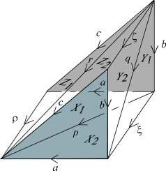
Fig. 5: the coefficient of the product of $\text{Tube}\Delta$

Let $V^{\Delta}(S^{1}\times S^{1})$ denote the subalgebra of $\text{Tube}\Delta$ defined by

$$V^{\Delta}(S^{1}\times S^{1})=\bigoplus\limits_{\rho,\zeta,\eta\in\Delta}\mathcal{H}_{\rho\eta}^{\zeta}\otimes\mathcal{H}_{\eta\rho}^{\zeta}.$$

We regard $S^{1}\times S^{1}$ as a quotient space obtained from a square by identifying the opposite sides. Then, $V^{\Delta}(S^{1}\times S^{1})$ is canonically identified with $V(S^{1}\times S^{1};\mathcal{K})$ as a vector space, where $\mathcal{K}$ is the locally ordered complex depicted in Figure 6 that gives a singular triangulation of $S^{1}\times S^{1}$.

Fig. 6: a distinguished triangulation $\mathcal{K}$ of $S^{1}\times S^{1}$

Under the identification $V^{\Delta}(S^{1}\times S^{1})=V(S^{1}\times S^{1};\mathcal{K})$, each element $X_{1}\otimes X_{2}$ in $V^{\Delta}(S^{1}\times S^{1})$ such that $X_{1}\in\mathcal{H}_{\rho a}^{p}$ and $X_{2}\in\mathcal{H}_{a\rho}^{p}$, corresponds to the color of $\mathcal{K}$ depicted in Figure 7.

Fig. 7: a color of $\mathcal{K}$

Now, we have two products on $V^{\Delta}(S^{1}\times S^{1})$. One is obtained from the product of the tube algebra $\text{Tube}\Delta$ by restricting to $V^{\Delta}(S^{1}\times S^{1})$. Another comes from the product of the fusion algebra $Z^{\Delta}(S^{1}\times S^{1})$. They are not same, but are closely related as follows.

Proposition 3.3.

Let $\Delta$ be a finite system of $\text{End}(M)_{0}$ obtained from a subfactor $N\subset M$ of an infinite factor $M$ with finite index and finite depth. Let $P:V^{\Delta}(S^{1}\times S^{1})\longrightarrow V^{\Delta}(S^{1}\times S^{1})$ be the conjugate linear map defined by $P(X_{1}\otimes X_{2})=X_{2}\otimes X_{1}$ for all $X_{1}\in\mathcal{H}_{\rho a}^{p}$ and $X_{2}\in\mathcal{H}_{a\rho}^{p}$. Then, the product $m_{\text{tube}}$ of the subalgebra $V^{\Delta}(S^{1}\times S^{1})$ of $\text{Tube}\Delta$ and the product $m_{\text{fusion}}$ of the fusion algebra associated to $Z^{\Delta}$ are related by the following commutative diagram.

$$\begin{CD}V^{\Delta}(S^{1}\times S^{1})\otimes V^{\Delta}(S^{1}\times S^{1})@>{m_{\text{tube}}}>{}>V^{\Delta}(S^{1}\times S^{1})\\ @V{P\otimes P}V{}V@V{}V{P}V\\ V^{\Delta}(S^{1}\times S^{1})\otimes V^{\Delta}(S^{1}\times S^{1})V^{\Delta}(S^{1}\times S^{1})\\ @V{u\otimes u}V{}V@V{}V{u}V\\ Z^{\Delta}(S^{1}\times S^{1})\otimes Z^{\Delta}(S^{1}\times S^{1})@>{m_{\text{fusion}}}>{}>Z^{\Delta}(S^{1}\times S^{1})\end{CD}$$

Here, $u$ is the universal arrow associated to $Z^{\Delta}(S^{1}\times S^{1})$ defined as in Lemma 2.1.

Proof. The $3$-holed sphere $Y$ in $\mathbb{R}^{3}$ is obtained as an identifying space of a regular heptagon. It is triangulated as in the right-hand side of Figure 8.

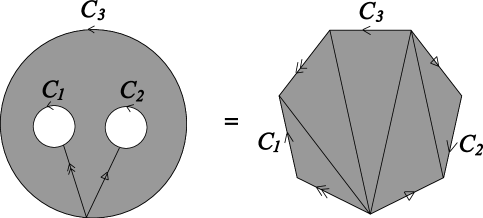
Fig. 8: a triangulation of $Y$

Therefore, the $3$-manifold $Y\times S^{1}$ is realized in $\mathbb{R}^{3}$ by the (singular) locally ordered complex $\tilde{\mathcal{K}}$ illustrated in Figure 9 (the cube with vertices $\underline{v}_{0},\underline{v}_{1},\underline{v}_{4},\underline{v}_{5}$, $\overline{v}_{0},\overline{v}_{1},\overline{v}_{4},\overline{v}_{5}$ and the cube with vertices $\underline{v}_{2},\underline{v}_{3},\underline{v}_{5},\underline{v}_{6}$, $\overline{v}_{2},\overline{v}_{3},\overline{v}_{5},\overline{v}_{6}$ are decomposed as product complexes, respectively).

Fig. 9: a triangulation of $Y\times S^{1}$

Hence, the product of the fusion algebra of $Z^{\Delta}$ is given by the linear map

$$Z_{\text{\scriptsize fusion}}^{\Delta}:Z^{\Delta}(S^{1}\times S^{1})\otimes Z^{\Delta}(S^{1}\times S^{1})\longrightarrow Z^{\Delta}(S^{1}\times S^{1}),$$

which is induced from the cobordism with triangulated boundary

$$W_{\text{\scriptsize fusion}}:=(Y\times S^{1};(C_{1}\times S^{1},\mathcal{K}_{1})\cup(C_{2}\times S^{1},\mathcal{K}_{2}),(C_{3}\times S^{1},\mathcal{K}_{3})),$$

where $\mathcal{K}_{i}\ (i=1,2,3)$ is the sub-complex of $\tilde{\mathcal{K}}$ such that

$$\mathcal{K}_{1} =K(|\underline{v_{0}}\ \overline{v_{0}}\ \overline{v_{1}}|)\cup K(|\underline{v_{0}}\ \underline{v_{1}}\ \overline{v_{1}}|),$$

$$\mathcal{K}_{2} =K(|\underline{v_{2}}\ \overline{v_{2}}\ \overline{v_{3}}|)\cup K(|\underline{v_{2}}\ \underline{v_{3}}\ \overline{v_{3}}|),$$

$$\mathcal{K}_{3} =K(|\underline{v_{4}}\ \overline{v_{4}}\ \overline{v_{6}}|)\cup K(|\underline{v_{4}}\ \underline{v_{6}}\ \overline{v_{6}}|).$$

We note that $\mathcal{K}_{i}$ is a copy of $\mathcal{K}$ for each $i=1,2,3$.

Let $\tilde{\mathcal{K}}_{1},\tilde{\mathcal{K}}_{2},\mathcal{L}$ be the sub-complexes of $\tilde{\mathcal{K}}$ depicted in Figure 10. The geometrical realizations of $\tilde{\mathcal{K}}_{1}$ and $\tilde{\mathcal{K}}_{2}$ are $S^{1}\times S^{1}\times[0,1]$, and the geometrical realization of $\mathcal{L}$ is $H\times S^{1}$, where $H$ is the quotient space obtained from a $2$-simplex by identifying its three vertices. Let $Z(S^{1}\times S^{1}\times[0,1];{}_{\rho,a,p,X_{1},X_{2}}^{\eta,b,q,Y_{1},Y_{2}})$ and $Z(H\times S^{1};a,{}_{\rho,p,X_{1},X_{2};\eta,q,Y_{1},Y_{2}}^{\zeta,r,Z_{1},Z_{2}})$ be the Turaev-Viro-Ocneanu invariants of $S^{1}\times S^{1}\times[0,1]$ triangulated by $\mathcal{K}\times[0,1]$ and of $H\times S^{1}$ triangulated by $\mathcal{L}$ assigned colors to their boundaries as in Figure 11, respectively.

Fig. 10: three sub-complexes of $\tilde{\mathcal{K}}$

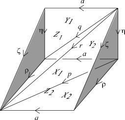
Fig. 11: triangulations of $S^{1}\times S^{1}\times[0,1]$ and $H\times S^{1}$ with colored boundaries

Fig. 12: colors of $\mathcal{K}_{1}$, $\mathcal{K}_{2}$ and $\mathcal{K}_{3}$

Then, the Turaev-Viro-Ocneanu invariant of $Y\times S^{1}$ triangulated by $\tilde{\mathcal{K}}$ assigned colors as in Figure 12 to $\mathcal{K}_{1},\ \mathcal{K}_{2},\ \mathcal{K}_{3}$ is given by

$$Z(Y\times S^{1};{}_{\rho,a,p,X_{1},X_{2};\eta,b,q,Y_{1},Y_{2}}^{\zeta,c,r,Z_{1},Z_{2}})=\dfrac{\lambda}{d(c)}\kern-8.99994pt\sum\limits_{\begin{subarray}{c}\rho^{\prime},\eta^{\prime},p^{\prime},q^{\prime}\in\Delta\\ X_{1}^{\prime}\in\mathcal{B}_{\rho^{\prime}c}^{p^{\prime}},X_{2}^{\prime}\in\mathcal{B}_{c\rho^{\prime}}^{p^{\prime}}\\ Y_{1}^{\prime}\in\mathcal{B}_{\eta^{\prime}c}^{q^{\prime}},Y_{2}^{\prime}\in\mathcal{B}_{c\eta^{\prime}}^{q^{\prime}}\end{subarray}}\kern-8.99994ptZ(H\times S^{1};c,{}_{\rho^{\prime},p^{\prime},X_{1}^{\prime},X_{2}^{\prime};\eta^{\prime},q^{\prime},Y_{1}^{\prime},Y_{2}^{\prime}}^{\zeta,r,Z_{1},Z_{2}})$$

$$\qquad\qquad\quad\qquad\times Z(S^{1}\times S^{1}\times[0,1];{}_{\rho,a,p,X_{1},X_{2}}^{\rho^{\prime},c,p^{\prime},X_{1}^{\prime},X_{2}^{\prime}})Z(S^{1}\times S^{1}\times[0,1];{}_{\eta,b,q,Y_{1},Y_{2}}^{\eta^{\prime},c,q^{\prime},Y_{1}^{\prime},Y_{2}^{\prime}}).$$

Since

and

$$Z(H\times S^{1};c,{}_{\rho^{\prime},p^{\prime},X_{1}^{\prime},X_{2}^{\prime};\eta^{\prime},q^{\prime},Y_{1}^{\prime},Y_{2}^{\prime}}^{\zeta,r,Z_{1},Z_{2}})=\dfrac{1}{d(c)}\overline{Z(D^{2}\times S^{1};{}_{c,\rho^{\prime},p^{\prime},X_{2}^{\prime},X_{1}^{\prime};c,\eta^{\prime},q^{\prime},Y_{2}^{\prime},Y_{1}^{\prime}}^{c,\zeta,r,Z_{2}^{\prime},Z_{1}^{\prime}})},$$

it follows that the following diagram commutes.

This implies that the diagram in the proposition is commutative. This completes the proof. ∎

Let $S$ and $T$ be the orientation preserving diffeomorphisms on $S^{1}\times S^{1}$ as in (3.1). We will compute the actions $Z^{\Delta}(S)$ and $Z^{\Delta}(T)$ on $Z^{\Delta}(S^{1}\times S^{1})$ by using the singular triangulation $\mathcal{K}$ of $S^{1}\times S^{1}$ depicted in Figure 6.

Lemma 3.4.

Let $\Delta$ be a finite system of $\text{End}(M)_{0}$ obtained from a subfactor $N\subset M$ of an infinite factor $M$ with finite index and finite depth. Let $\tilde{S}_{\#}:V^{\Delta}(S^{1}\times S^{1})\longrightarrow V^{\Delta}(S^{1}\times S^{1})$ and $\tilde{T}_{\#}^{-1}:V^{\Delta}(S^{1}\times S^{1})\longrightarrow V^{\Delta}(S^{1}\times S^{1})$ be the $\mathbb{C}$-linear maps defined by

$$\tilde{S}_{\#}(X_{1}\otimes X_{2}) =\sum\limits_{\begin{subarray}{c}r\in\Delta\\ Z_{1}\in\mathcal{B}_{\bar{a}\rho}^{r}\\ Z_{2}\in\mathcal{B}_{\rho\bar{a}}^{r}\end{subarray}}\kern-5.69046pt\dfrac{\sqrt{d(p)d(r)}}{d(\rho)}Z_{2}^{\ast}\tilde{X}_{2}^{\ast}\bar{a}(\hat{X}_{1})Z_{1}\ Z_{1}\otimes Z_{2},$$

$$\tilde{T}_{\#}^{-1}(X_{1}\otimes X_{2}) =\sum\limits_{\begin{subarray}{c}r\in\Delta\\ Z_{1}\in\mathcal{B}_{\rho p}^{r}\\ Z_{2}\in\mathcal{B}_{p\rho}^{r}\end{subarray}}\kern-5.69046pt\dfrac{\sqrt{d(a)d(r)}}{d(p)}Z_{2}^{\ast}X_{1}^{\ast}\rho(X_{2})Z_{1}\ Z_{1}\otimes Z_{2}$$

for all $X_{1}\in\mathcal{B}_{\rho a}^{p}$ and $X_{2}\in\mathcal{B}_{a\rho}^{p}$. Then, the actions $Z^{\Delta}(S)$ and $Z^{\Delta}(T)$ on $Z^{\Delta}(S^{1}\times S^{1})$ are determined by the following commutative diagrams.

$$\begin{CD}V^{\Delta}(S^{1}\times S^{1})@>{\tilde{S}_{\#}}>{}>V^{\Delta}(S^{1}\times S^{1})\\ @V{u}V{}V@V{}V{u}V\\ Z^{\Delta}(S^{1}\times S^{1})@>{Z^{\Delta}(S)}>{}>Z^{\Delta}(S^{1}\times S^{1}),\end{CD}$$ (3.2)

$$\begin{CD}V^{\Delta}(S^{1}\times S^{1})@>{\tilde{T}_{\#}^{-1}}>{}>V^{\Delta}(S^{1}\times S^{1})\\ @V{u}V{}V@V{}V{u}V\\ Z^{\Delta}(S^{1}\times S^{1})@>{Z^{\Delta}(T)^{-1}}>{}>Z^{\Delta}(S^{1}\times S^{1})\end{CD}$$ (3.3)

Here, $u$ is the universal arrow associated to $Z^{\Delta}(S^{1}\times S^{1})$ defined as in Lemma 2.1.

Proof. Let $\mathcal{K}$, $\mathcal{L}_{1}$ and $\mathcal{L}_{2}$ be the locally ordered complexes depicted in Figure 13 that give singular triangulations of $S^{1}\times S^{1}$ (the opposite sides are identified). By considering the lifts of $S$ and $T$ to the universal covering

$$\mathbb{R}^{2}\longrightarrow S^{1}\times S^{1},\ (x,y)\longmapsto(\text{exp}(2\pi iy),\text{exp}(2\pi ix)),$$

we see that $S$ and $T^{-1}$ are simplicial maps from $\mathcal{K}$ to $\mathcal{L}_{1}$ and from $\mathcal{K}$ to $\mathcal{L}_{2}$, respectively.

Fig. 13: three triangulations of $S^{1}\times S^{1}$

So, for the color depicted in Figure 7, we have

Let $S_{\#}$ and $T_{\#}^{-1}$ be the linear maps from $V(S^{1}\times S^{1};\mathcal{K})$ to $V(S^{1}\times S^{1};\mathcal{K})$ defined by

$$S_{\#}=\Phi_{\mathcal{L}_{1},\mathcal{K}}\circ\Phi(S),\qquad T_{\#}^{-1}=\Phi_{\mathcal{L}_{2},\mathcal{K}}\circ\Phi(T^{-1}).$$

Then we have

where $Z(\mathcal{T}_{1};{}_{\rho,a,p,X_{1},X_{2}}^{\eta,b,q,Y_{1},Y_{2}})$ is the Turaev-Viro-Ocneanu invariant of $(S^{1}\times S^{1})\times[0,1]$ which boundary is triangulated by $\mathcal{K}$ and $\mathcal{L}_{1}$ assigned to its boundary the color depicted as in the left-hand side of Figure 14, and $Z(\mathcal{T}_{2};{}_{\rho,a,p,X_{1},X_{2}}^{\eta,b,q,Y_{1},Y_{2}})$ is the Turaev-Viro-Ocneanu invariant of $(S^{1}\times S^{1})\times[0,1]$ which boundary is triangulated by $\mathcal{K}$ and $\mathcal{L}_{2}$ assigned to its boundary the color depicted as in the right-hand side of Figure 14.

Fig. 14: two triangulations $\mathcal{T}_{1}$ and $\mathcal{T}_{2}$ of $S^{1}\times S^{1}\times[0,1]$

By tetrahedral symmetry on quantum $6j$-symbols, it can be proved that

$$Z(\mathcal{T}_{1};{}_{\rho,a,p,X_{1},X_{2}}^{\eta,b,q,Y_{1},Y_{2}})=Z(\mathcal{T}_{2};{}_{\bar{a},p,\rho,\tilde{X}_{2},\hat{X}_{1}}^{\eta,b,q,Y_{1},Y_{2}}).$$

Let $(\mathcal{T}_{3};\mathcal{L}_{2},\mathcal{K})$ be the cobordism obtained by gluing one tetrahedron to the bottom of $\mathcal{K}\times[0,1]$. Then, we have

$$Z(\mathcal{T}_{2};{}_{\rho,a,p,X_{1},X_{2}}^{\eta,b,q,Y_{1},Y_{2}})=Z(\mathcal{T}_{3};{}_{\rho,a,p,X_{1},X_{2}}^{\eta,b,q,Y_{1},Y_{2}}),$$

since the cobordism $(\mathcal{T}_{2};\mathcal{L}_{2},\mathcal{K})$ is isomorphic to the cobordism $(\mathcal{T}_{3};\mathcal{L}_{2},\mathcal{K})$ (see Figure 15).

Fig. 15: an isomorphism between $(\mathcal{T}_{2};\mathcal{L}_{2},\mathcal{K})$ and $(\mathcal{T}_{3};\mathcal{L}_{2},\mathcal{K})$

Since

it follows that

This implies that $S_{\#}=\Phi_{Id_{\mathcal{K},\mathcal{K}}}\circ\tilde{S}_{\#}$, and whence, the diagram (3.2) commutes.

By a similar argument, it is also proved that

and whence, $T^{-1}_{\#}=\Phi_{Id_{\mathcal{K},\mathcal{K}}}\circ\tilde{T}_{\#}^{-1}$. This proves that the diagram (3.3) commutes. ∎

We note that the group $SL(2,\mathbb{Z})$ is not only generated by $S=\begin{pmatrix}0&1\\ -1&0\end{pmatrix}$ and $T=\begin{pmatrix}1&0\\ 1&1\end{pmatrix}$, but also generated by $S^{\prime}=\begin{pmatrix}0&-1\\ 1&0\end{pmatrix}$ and $T^{\prime}=\begin{pmatrix}1&1\\ 0&1\end{pmatrix}$. The matrices $S^{\prime}$ and $T^{\prime}$ correspond to the orientation preserving diffeomorphisms from $S^{1}\times S^{1}$ to $S^{1}\times S^{1}$ defined by $S^{\prime}(z,w)=(w,\bar{z})$ and $T^{\prime}(z,w)=(z,zw)$ for all $(z,w)\in S^{1}\times S^{1}$, respectively. Since $S^{\prime}$ and $T^{\prime}$ has also the relations $(S^{\prime})^{4}=I,\ (S^{\prime}T^{\prime})^{3}=(S^{\prime})^{2}$, we have a group isomorphism $Q:SL(2,\mathbb{Z})\longrightarrow SL(2,\mathbb{Z})$ such that $Q(S)=S^{\prime}$ and $Q(T)=T^{\prime}$.

Lemma 3.5.

Let $\Delta$ be a finite system of $\text{End}(M)_{0}$ obtained from a subfactor $N\subset M$ of an infinite factor $M$ with finite index and finite depth. Let $\bar{P}:Z^{\Delta}(S^{1}\times S^{1})\longrightarrow Z^{\Delta}(S^{1}\times S^{1})$ be the conjugate linear isomorphism induced from $P$ defined as in Proposition 3.3. Then, the following diagram commutes for all $R\in SL(2,\mathbb{Z})$.

$$\begin{CD}Z^{\Delta}(S^{1}\times S^{1})@>{Z^{\Delta}(R)}>{}>Z^{\Delta}(S^{1}\times S^{1})\\ @V{\bar{P}}V{}V@V{}V{\bar{P}}V\\ Z^{\Delta}(S^{1}\times S^{1})@>{Z^{\Delta}(R^{\prime})}>{}>Z^{\Delta}(S^{1}\times S^{1})\end{CD}$$

Here, $R^{\prime}$ denotes the image of $R$ by the group isomorphism $Q:SL(2,\mathbb{Z})\longrightarrow SL(2,\mathbb{Z})$.

Proof. Let $\mathcal{K}$, $\mathcal{L}_{1}^{\prime}$ and $\mathcal{L}_{2}^{\prime}$ be the locally ordered complexes depicted in Figure 16 that give singular triangulations of $S^{1}\times S^{1}$ (the opposite sides are identified).

Fig. 16: three triangulations of $S^{1}\times S^{1}$

Since $S^{\prime}$ and ${T^{\prime}}^{-1}$ are simplicial maps from $\mathcal{K}$ to $\mathcal{L}_{1}^{\prime}$ and from $\mathcal{K}$ to $\mathcal{L}_{2}^{\prime}$, respectively, we have

Thus, we have

where $Z(\mathcal{T}_{1}^{\prime};{}_{\rho,a,p,X_{1},X_{2}}^{\eta,b,q,Y_{1},Y_{2}})$ and $Z(\mathcal{T}_{2}^{\prime};{}_{\rho,a,p,X_{1},X_{2}}^{\eta,b,q,Y_{1},Y_{2}})$ are the Turaev-Viro-Ocneanu invariants of $S^{1}\times S^{1}\times[0,1]$ based on the triangulations $\mathcal{T}_{1}^{\prime}$ and $\mathcal{T}_{2}^{\prime}$ with colored boundaries as in Figure 17, respectively.

Fig. 17: two triangulations $\mathcal{T}_{1}^{\prime}$ and $\mathcal{T}_{2}^{\prime}$ of $S^{1}\times S^{1}\times[0,1]$

Since

$$Z(\mathcal{T}_{1}^{\prime};{}_{\rho,a,p,X_{1},X_{2}}^{\eta,b,q,Y_{1},Y_{2}})=\overline{Z(\mathcal{T}_{1};{}_{a,\rho,p,X_{2},X_{1}}^{b,\eta,q,Y_{2},Y_{1}})}\text{ and }Z(\mathcal{T}_{2}^{\prime};{}_{\rho,a,p,X_{1},X_{2}}^{\eta,b,q,Y_{1},Y_{2}})=\overline{Z(\mathcal{T}_{2};{}_{a,\rho,p,X_{2},X_{1}}^{b,\eta,q,Y_{2},Y_{1}})},$$

the following diagrams commute.

$$\begin{CD}Z^{\Delta}(S^{1}\times S^{1})@>{Z^{\Delta}(S)}>{}>Z^{\Delta}(S^{1}\times S^{1})\\ @V{\bar{P}}V{}V@V{}V{\bar{P}}V\\ Z^{\Delta}(S^{1}\times S^{1})@>{Z^{\Delta}(S^{\prime})}>{}>Z^{\Delta}(S^{1}\times S^{1}),\end{CD}\quad\begin{CD}Z^{\Delta}(S^{1}\times S^{1})@>{Z^{\Delta}(T^{-1})}>{}>Z^{\Delta}(S^{1}\times S^{1})\\ @V{\bar{P}}V{}V@V{}V{\bar{P}}V\\ Z^{\Delta}(S^{1}\times S^{1})@>{Z^{\Delta}({T^{\prime}}^{-1})}>{}>Z^{\Delta}(S^{1}\times S^{1})\end{CD}$$

This completes the proof. ∎

4 .  Correspondence between Izumi’s Tube Algebra and Ocneanu’s Tube Algebra

Izumi [8] translated the notion of Ocneanu’s tube algebra [12] into the language of sectors, and gave explicit formulas of the tube algebra operations and of the $S$- and $T$-matrices. He also showed that $SL(2,\mathbb{Z})$ acts on the center of the tube algebra and that the Verlinde identity holds. It is a natural question whether Izumi’s tube algebra and Ocneanu’s one are isomorphic as algebras, and whether the centers of these tube algebras are isomorphic as algebras commuting with $SL(2,\mathbb{Z})$-actions. In this section, we show that there exists a conjugate linear isomorphism between the center of Izumi’s tube algebra and that of Ocneanu’s one, which preserves products of algebras and commutes with $SL(2,\mathbb{Z})$-actions.

Let us recall the definition of the tube algebra in sector theory, which was introduced by Izumi [8]. Let $\Delta$ be a finite system of $\text{End}(M)_{0}$ obtained from a subfactor $N\subset M$ of an infinite factor $M$ with finite index and finite depth. The tube algebra $\text{Tube}_{I}\Delta$ introduced by Izumi is a $C^{\ast}$-algebra defined as follows. As a $\mathbb{C}$-vector space, $\text{Tube}_{I}\Delta$ is spanned by

$$\{(\xi\zeta|X|\zeta\eta)\ |\ \xi,\zeta,\eta\in\Delta,\ X\in(\xi\zeta,\zeta\eta)\}.$$

The product of $\text{Tube}_{I}\Delta$ is given by

$$(\xi\zeta|X|\zeta\eta)\cdot(\xi^{\prime}\zeta^{\prime}|Y|\zeta^{\prime}\eta^{\prime})=\delta_{\eta,\xi^{\prime}}\sum\limits_{\nu\prec\zeta\zeta^{\prime}}\sum\limits_{A\in\mathcal{B}_{\zeta\zeta^{\prime}}^{\nu}}(\xi\nu|A^{\ast}\zeta(Y)X\xi(A)|\nu\eta^{\prime}),$$

where $\delta_{\eta,\xi^{\prime}}$ is Kronecker’s delta and $\nu\prec\zeta\zeta^{\prime}$ means that $\nu$ appears in the product $\zeta\zeta^{\prime}$ as an irreducible component. The $\ast$-structure is given by

$$(\xi\zeta|X|\zeta\eta)^{\ast}=d(\zeta)(\eta\bar{\zeta}|\bar{\zeta}(\xi(\overline{R}_{\zeta}^{\ast})X^{\ast})R_{\zeta}|\bar{\zeta}\xi).$$

Izumi showed that $SL(2,\mathbb{Z})$ acts on the center $\mathcal{Z}(\text{Tube}_{I}\Delta)$ of $\text{Tube}_{I}\Delta$ [8]. The action is given by

$$S^{\prime}_{\Delta}(\xi\eta|X|\eta\xi)=d(\xi)(\bar{\eta}\xi|R_{\eta}^{\ast}\bar{\eta}(X\xi(\bar{R}_{\eta}))|\xi\bar{\eta}),$$

$$T^{\prime}_{\Delta}(\xi\eta|X|\eta\xi)=\sum\limits_{\zeta\in\Delta}d(\zeta)(\zeta\bar{\zeta}|R_{\zeta}\bar{R}_{\zeta}^{\ast}|\bar{\zeta}\zeta)\cdot(\xi\eta|X|\eta\xi)$$

for $S^{\prime}=\begin{pmatrix}0&-1\\ 1&0\end{pmatrix}$ and $T^{\prime}=\begin{pmatrix}1&1\\ 0&1\end{pmatrix}$. In particular, the action of ${T^{\prime}}^{-1}$ is given by

$${T^{\prime}}^{-1}_{\Delta}(\xi\eta|X|\eta\xi)=(\xi p|X_{1}^{\ast}\xi(X_{2})|p\xi)$$

for $X=X_{2}X_{1}^{\ast},\ X_{1}\in(p,\xi\eta),\ X_{2}\in(p,\eta\xi)$ and $p,\xi,\eta\in\Delta$.

Izumi’s tube algebra is isomorphic to Ocneanu’s one in the following sense.

Theorem 4.1.

Let $\Delta$ be a finite system of $\text{End}(M)_{0}$ obtained from a subfactor $N\subset M$ of an infinite factor $M$ with finite index and finite depth. Let $\varphi:\text{Tube}\Delta\longrightarrow\text{Tube}_{I}\Delta$ be the $\mathbb{C}$-linear map defined by

$$\varphi(X_{1}\otimes X_{2})=w^{-\frac{1}{2}}\biggl{(}\frac{d(a)}{d(p)d(\rho)}\biggr{)}^{1/4}\biggl{(}\frac{d(a)}{d(p)d(\xi)}\biggr{)}^{1/4}\ (\rho a|X_{2}X_{1}^{\ast}|a\rho)$$

for $X_{1}\otimes X_{2}\in\mathcal{H}_{\rho a}^{p}\otimes\mathcal{H}_{a\xi}^{p}$. Then, $\varphi$ is an algebra isomorphism. Furthermore, the restriction of $\varphi$ to the subspace $V^{\Delta}(S^{1}\times S^{1})$ gives rise to an $\mathbb{C}$-linear isomorphism $\bar{\varphi}:Z^{\Delta}(S^{1}\times S^{1})\longrightarrow\mathcal{Z}(\text{Tube}_{I}\Delta)$ such that the following diagram commutes for all $R\in SL(2,\mathbb{Z})$.

$$\begin{CD}Z^{\Delta}(S^{1}\times S^{1})@>{Z^{\Delta}(R)}>{}>Z^{\Delta}(S^{1}\times S^{1})\\ @V{\bar{\varphi}}V{}V@V{}V{\bar{\varphi}}V\\ \mathcal{Z}(\text{Tube}_{I}\Delta)@>{Q(R)_{\Delta}}>{}>\mathcal{Z}(\text{Tube}_{I}\Delta)\end{CD}$$

Here, $Q:SL(2,\mathbb{Z})\longrightarrow SL(2,\mathbb{Z})$ is the group isomorphism satisfying $Q(S)=S^{\prime}$ and $Q(T)=T^{\prime}$.

To prove the above theorem, we need the following theorem which was announced by Ocneanu [12] and was proved in [10]. This is an important theorem about the tube algebra.

Theorem 4.2 ([12, 10]).

Let $\Delta$ be a finite system of $\text{End}(M)_{0}$ obtained from a subfactor $N\subset M$ of an infinite factor $M$ with finite index and finite depth. Then,

$$Z^{\Delta}(S^{1}\times S^{1})\cong\mathcal{Z}(\text{Tube}\Delta)$$

as vector spaces.

Proof of Theorem 4.1. First, we show that $\varphi$ is a homomorphism of algebras. For $X_{1}\otimes X_{2}\in\mathcal{H}_{\rho a}^{p}\otimes\mathcal{H}_{a\xi}^{p}$ and $Y_{1}\otimes Y_{2}\in\mathcal{H}_{\eta b}^{q}\otimes\mathcal{H}_{b\zeta}^{q}$, the product in $\text{Tube}\Delta$ is given by

$$(X_{1}\otimes X_{2})\cdot(Y_{1}\otimes Y_{2})= \delta_{\xi,\eta}\lambda^{-\frac{1}{2}}\sqrt{\frac{d(a)d(b)d(r)}{d(c)d(p)d(q)d(\xi)}}$$

$$\times\sum\limits_{\begin{subarray}{c}Z_{1}\in\mathcal{B}_{\rho c}^{r}\\ Z_{2}\in\mathcal{B}_{c\zeta}^{r}\end{subarray}}Z_{2}^{\ast}(\sum\limits_{A\in\mathcal{B}_{ab}^{c}}A^{\ast}a(Y_{2}Y_{1}^{\ast})X_{2}X_{1}^{\ast}\xi(A))Z_{1}\ (Z_{1}\otimes Z_{2}).$$

Thus, we have

$$d(\rho)^{1/4}d(\zeta)^{1/4}\varphi((X_{1}\otimes X_{2})\cdot(Y_{1}\otimes Y_{2}))$$

$$= \delta_{\xi,\eta}\frac{\lambda^{-1}}{\sqrt{d(\xi)}}\sqrt{\frac{d(a)d(b)}{d(p)d(q)}}\sum\limits_{\begin{subarray}{c}Z_{1}\in\mathcal{B}_{\rho c}^{r}\\ Z_{2}\in\mathcal{B}_{c\zeta}^{r}\end{subarray}}Z_{2}^{\ast}(\sum\limits_{A\in\mathcal{B}_{ab}^{c}}A^{\ast}a(Y_{2}Y_{1}^{\ast})X_{2}X_{1}^{\ast}\xi(A))Z_{1}\ (\xi c|Z_{2}Z_{1}^{\ast}|c\xi)$$

$$= \delta_{\xi,\eta}\frac{\lambda^{-1}}{\sqrt{d(\xi)}}\sqrt{\frac{d(a)d(b)}{d(p)d(q)}}\sum_{\begin{subarray}{c}c,r\in\Delta\\ c\prec ab\\ r\prec c\xi\end{subarray}}\sum\limits_{\begin{subarray}{c}Z_{1}\in\mathcal{B}_{\rho c}^{r}\\ Z_{2}\in\mathcal{B}_{c\zeta}^{r}\end{subarray}}\sum\limits_{A\in\mathcal{B}_{ab}^{c}}\ (\xi c|Z_{2}Z_{2}^{\ast}A^{\ast}a(Y_{2}Y_{1}^{\ast})X_{2}X_{1}^{\ast}\xi(A)Z_{1}Z_{1}^{\ast}|c\xi)$$

$$= \delta_{\xi,\eta}\frac{\lambda^{-1}}{\sqrt{d(\xi)}}\sqrt{\frac{d(a)d(b)}{d(p)d(q)}}\sum_{\begin{subarray}{c}c\in\Delta\\ c\prec ab\end{subarray}}\sum\limits_{A\in\mathcal{B}_{ab}^{c}}(\xi c|A^{\ast}a(Y_{2}Y_{1}^{\ast})X_{2}X_{1}^{\ast}\xi(A)|c\xi)$$

$$= d(\rho)^{1/4}d(\zeta)^{1/4}\varphi(X_{1}\otimes X_{2})\varphi(Y_{1}\otimes Y_{2}).$$

Hence, $\varphi$ preserves the products. It is clear that $\varphi$ is bijective. Thus, $\varphi$ is an algebra isomorphism.

Let $\varphi^{\prime}$ be the algebra isomorphism from the center of $\text{Tube}\Delta$ to the center of $\text{Tube}_{I}\Delta$ induced from $\varphi$. We regard $Z^{\Delta}(S^{1}\times S^{1})$ as a subspace of the center $\mathcal{Z}(\text{Tube}\Delta)$, and denote by $\bar{\varphi}$ the restriction of $\varphi^{\prime}$ to $Z^{\Delta}(S^{1}\times S^{1})$. We will show that $\bar{\varphi}$ induces an $SL(2,\mathbb{Z})$-equivariant map from $Z^{\Delta}(S^{1}\times S^{1})$ to $\mathcal{Z}(\text{Tube}_{I}\Delta)$ in the sense of the statement in the theorem. By Lemma 3.4, for $X_{1}\in\mathcal{B}_{\rho a}^{p}$ and $X_{2}\in\mathcal{B}_{a\rho}^{p}$ we have

$$\tilde{S}_{\#}(X_{1}\otimes X_{2}) =\sum\limits_{\begin{subarray}{c}r\in\Delta\\ Z_{1}\in\mathcal{B}_{\bar{a}\rho}^{r}\\ Z_{2}\in\mathcal{B}_{\rho\bar{a}}^{r}\end{subarray}}\kern-5.69046pt\dfrac{\sqrt{d(p)d(r)}}{d(\rho)}Z_{2}^{\ast}\tilde{X}_{2}^{\ast}\bar{a}(\hat{X}_{1})Z_{1}\ Z_{1}\otimes Z_{2},$$

$$\tilde{T}_{\#}^{-1}(X_{1}\otimes X_{2}) =\sum\limits_{\begin{subarray}{c}r\in\Delta\\ Z_{1}\in\mathcal{B}_{\rho p}^{r}\\ Z_{2}\in\mathcal{B}_{p\rho}^{r}\end{subarray}}\kern-5.69046pt\dfrac{\sqrt{d(a)d(r)}}{d(p)}Z_{2}^{\ast}X_{1}^{\ast}\rho(X_{2})Z_{1}\ Z_{1}\otimes Z_{2}.$$

It follows immediately from the second equation that $\varphi^{\prime}\circ\tilde{T}_{\#}^{-1}={T_{\Delta}^{\prime}}^{-1}\circ\varphi^{\prime}$. Since

$$\dfrac{1}{d(\rho)}Z_{2}^{\ast}\tilde{X}_{2}^{\ast}\bar{a}(\hat{X}_{1})Z_{1} =\dfrac{1}{d(\rho)}\dfrac{d(\rho)d(a)}{d(p)}Z_{2}^{\ast}(\bar{a}(X_{2}^{\ast})R_{a})^{\ast}\bar{a}(X_{1}^{\ast}\rho(\overline{R}_{a}))Z_{1}$$

$$=\dfrac{d(a)}{d(p)}Z_{2}^{\ast}R_{a}^{\ast}\bar{a}(X_{2})\bar{a}(X_{1}^{\ast}\rho(\overline{R}_{a}))Z_{1}$$

$$=\dfrac{d(a)}{d(p)}Z_{2}^{\ast}R_{a}^{\ast}\bar{a}(X_{2}X_{1}^{\ast}\rho(\overline{R}_{a}))Z_{1}$$

$$=\dfrac{d(a)}{d(p)d(\rho)}Z_{2}^{\ast}S_{\Delta}^{\prime}(\rho a|X_{2}X_{1}^{\ast}|a\rho)Z_{1},$$

we see also that $\varphi^{\prime}\circ\tilde{S}_{\#}=S_{\Delta}^{\prime}\circ\varphi^{\prime}$. Thus, $\bar{\varphi}$ is an $SL(2,\mathbb{Z})$-equivariant homomorphism.

Since $\dim Z^{\Delta}(S^{1}\times S^{1})=\dim\mathcal{Z}(\text{Tube}_{I}\Delta)$ by Theorem 4.2 and $\bar{\varphi}$ is injective, it follows that $\bar{\varphi}$ is an $SL(2,\mathbb{Z})$-equivariant isomorphism. This completes the proof. ∎

By Theorem 4.1, Proposition 3.3 and Lemma 3.5, we have :

Corollary 4.3.

Let $\Delta$ be a finite system of $\text{End}(M)_{0}$ obtained from a subfactor $N\subset M$ of an infinite factor $M$ with finite index and finite depth. Let $\varphi:\text{Tube}\Delta\longrightarrow\text{Tube}_{I}\Delta$ be the algebra isomorphism defined as in the above theorem, and $P:V^{\Delta}(S^{1}\times S^{1})\longrightarrow V^{\Delta}(S^{1}\times S^{1})$ the conjugate linear isomorphism defined as in Proposition 3.3. Then, the composition $\varphi\circ P:V^{\Delta}(S^{1}\times S^{1})\longrightarrow\text{Tube}_{I}\Delta$ induces a conjugate linear isomorphism $\phi:Z^{\Delta}(S^{1}\times S^{1})\longrightarrow\mathcal{Z}(\text{Tube}_{I}\Delta)$, which preserves the products of these two algebras and commutes with the actions of $SL(2,\mathbb{Z})$.

Remark 4.4.

Izumi has introduced an inner product $\langle\ \ ,\ \ \rangle_{\text{Tube}}$ on $\text{Tube}_{I}\Delta$ as follows [8].

$$\langle(\xi\zeta|X|\zeta\eta),(\xi^{\prime}\zeta^{\prime}|Y|\zeta^{\prime}\eta^{\prime})\rangle_{\text{Tube}}=\delta_{\xi,\xi^{\prime}}\delta_{\zeta,\zeta^{\prime}}d(\xi)^{2}R_{\zeta}^{\ast}\bar{\zeta}(XY^{\ast})R_{\zeta}.$$

Let $\{v_{i}\}_{i=0}^{m}$ be a Verlinde basis of $Z^{\Delta}(S^{1}\times S^{1})$, and $\{w_{i}\}_{i=1}^{m}$ the primitive idempotents in the fusion algebra $Z^{\Delta}(S^{1}\times S^{1})$ obtained from $\{v_{i}\}_{i=0}^{m}$ by applying the transformation $S$ (see Remarks 3.2). Then, the basis $\{\frac{\sqrt{\lambda}}{d_{i}}\phi(w_{i})\}_{i=0}^{m}$ is orthonormal with respect to the inner product $\langle\ \ ,\ \ \rangle_{\text{Tube}}$, where $d_{i}=\lambda S_{0i}$ and $Z^{\Delta}(S)v_{i}=\sum_{j}{S}_{ji}v_{j}$ [8].

On the other hand, since the Verlinde basis $\{v_{i}\}_{i=0}^{m}$ is orthonormal with respect to the inner product $\langle\ \ ,\ \ \rangle_{\text{TQFT}}$ based on the TQFT defined as in Section 3, and $Z^{\Delta}(S)$ is unitary with respect to the inner product $\langle\ \ ,\ \ \rangle_{\text{TQFT}}$, we have

$$\langle\frac{\sqrt{\lambda}}{d_{i}}w_{i},\ \frac{\sqrt{\lambda}}{d_{j}}w_{j}\rangle_{\text{TQFT}}= \langle\frac{1}{\sqrt{\lambda}S_{0i}}w_{i},\ \frac{1}{\sqrt{\lambda}S_{0j}}w_{j}\rangle_{\text{TQFT}}$$

$$= \frac{1}{\lambda}\langle Z^{\Delta}(S)^{\ast}(v_{i}),Z^{\Delta}(S)^{\ast}(v_{j})\rangle_{\text{TQFT}}$$

$$= \frac{1}{\lambda}\langle v_{i},v_{j}\rangle_{\text{TQFT}}$$

$$= \frac{1}{\lambda}\delta_{ij}.$$

Therefore, $\phi$ does not preserve the inner products.

5 .  Calculations of Turaev-Viro-Ocneanu invariants of Basic $3$-manifolds

Izumi explicitly gave an action of $SL(2,\mathbb{Z})$ on the center of the tube algebra in the language of sectors, and derived some formulas on Turaev-Viro-Ocneanu invariants of lens spaces by applying formulas in [16] to subfactors constructed by his method [8, 9]. In the previous section, we established a rigorous correspondence between the $S$- and $T$-matrices in Izumi’s sector theory and the ones in Turaev-Viro-Ocneanu $(2+1)$-dimensional TQFT. Via this correspondence and the Dehn surgery formula of the Turaev-Viro-Ocneanu invariant, we can compute the Turaev-Viro-Ocneanu invariants of $3$-manifolds in the language of sectors. In this section, using techniques on sectors due to Izumi [8, 9], we compute the Turaev-Viro-Ocneanu invariants from several subfactors for basic $3$-manifolds including lens spaces and Brieskorn $3$-manifolds. One of the most important result is that the homology $3$-sphere $S^{3}$ and the Poincaré homology $3$-sphere $\Sigma(2,3,5)$ are distinguished by the Turaev-Viro-Ocneanu invariant from the exotic subfactor constructed by Haagerup and Asaeda [4, 1], and $L(p,1)$ and $L(p,2)$ are distinguished by the Turaev-Viro-Ocneanu invariant from a generalized $E_{6}$-subfactor with $\mathbb{Z}/p\mathbb{Z}$ for $p=3,5$.

Let $\Delta$ be a finite system of $\text{End}(M)_{0}$ obtained from a subfactor $N\subset M$ of an infinite factor $M$ with finite index and finite depth. Since any finite dimensional $C^{*}$-algebra is semisimple, we may assume that ${\rm Tube}\Delta=\oplus_{i=0}^{r}\text{M}_{n_{i}}({\mathbb{C}})$ as algebras, where $\text{M}_{n_{i}}(\mathbb{C})$ is the set of $n_{i}\times n_{i}$-matrices over $\mathbb{C}$. From each direct summand of ${\rm Tube}\Delta=\oplus_{i=0}^{r}\text{M}_{n_{i}}(\mathbb{C})$, we pick up a minimal projection $p_{i}$. Then, we have proved that $\{p_{i}\}_{i=0}^{r}$ is a Verlinde basis of $Z^{\Delta}(S^{1}\times S^{1})$ in the sense of Definition 3.1 [10]. Thus, we have :

Theorem 5.1 ([10]).

Let $\Delta$ be a finite system of $\text{End}(M)_{0}$ obtained from a subfactor $N\subset M$ of an infinite factor $M$ with finite index and finite depth. Then, there exists a Verlinde basis of $Z^{\Delta}(S^{1}\times S^{1})$ in the sense of Definition 3.1.

Let us recall the Dehn surgery formula of $Z(M)$ [20, 10]. Let $Z$ be a $(2+1)$-dimensional TQFT, and $\{v_{i}\}_{i=0}^{m}$ a basis of $Z(S^{1}\times S^{1})$.

We introduce a framed link invariant in the following way. Let $L=L_{1}\cup\cdots\cup L_{r}$ be a framed link with $r$-components in the 3-sphere $S^{3}$, and $h_{i}:D^{2}\times S^{1}\longrightarrow N(L_{i})$ be the framing of $L_{i}$ for each $i\in\{1,\cdots,r\}$, where $N(L_{i})$ denotes the tubular neighborhood of $L_{i}$. We fix an orientation for $\partial N(L_{i})$ such that $j_{i}:=h_{i}|_{\partial D^{2}\times S^{1}}:S^{1}\times S^{1}\longrightarrow\partial N(L_{i})$ is orientation preserving. Since the orientation for $N(L_{i})$ is not compatible with the orientation for the link exterior $X:=\overline{S^{3}-N(L_{1})\cup\cdots\cup N(L_{r})}$, we can consider the cobordism parametrized boundary ${\cal W}_{L}:=(X;\coprod\limits_{i=1}^{r}j_{i},\emptyset)$ (See [10] for detail). This cobordism induces a $\mathbb{C}$-linear map $Z_{{\cal W}_{L}}:\bigotimes\limits_{i=1}^{r}Z(S^{1}\times S^{1})\longrightarrow\mathbb{C}$. It is easy to see that for each $i_{1},\cdots,i_{r}=0,1,\cdots,m$ the complex number $J(L;i_{1},\cdots,i_{r}):=Z_{{\cal W}_{L}}(v_{i_{1}}\otimes\cdots\otimes v_{i_{r}})$ is a framed link invariant of $L$. In this setting, we proved the following proposition.

Proposition 5.2 (Dehn surgery formula [10]).

Let $Z$ be a (2+1)-dimensional TQFT and $\{v_{i}\}_{i=0}^{m}$ a basis of the fusion algebra $Z(S^{1}\times S^{1})$ such that $v_{0}$ is the identity element in the fusion algebra. Let $M$ be a closed oriented 3-manifold obtained from $S^{3}$ by Dehn surgery along a framed link $L=L_{1}\cup\cdots\cup L_{r}$. Then, the 3-manifold invariant $Z(M)$ is given by the formula

$$Z(M)=\sum_{i_{1},\cdots,i_{r}=0}^{m}S_{i_{1}0}\cdots S_{i_{r}0}J(L;i_{1},\cdots,i_{r}),$$

where $S_{ji}\in\mathbb{C}$, $i,j=0,1,\cdots,m$ are defined by $Z(S)v_{i}=\sum_{j=0}^{m}S_{ji}v_{j}$, and $S:S^{1}\times S^{1}\longrightarrow S^{1}\times S^{1}$ is the orientation preserving diffeomorphism defined by $S(z,w)=(\bar{w},z)$ for all $(z,w)\in S^{1}\times S^{1}$.

This is a quite general formula which is a conclusion of the axioms of $(2+1)$-dimensional TQFT. The right-hand side of this formula looks very similar to the formula of the Reshetikhin-Turaev invariant of closed 3-manifolds, although many things are missing in the above general formula, compared to the Reshetikhin-Turaev formula [13]. (See [10, 15] for more details on the Dehn surgery formula and its applications.)

From Proposition 5.2, if we want to compute the Turaev-Viro-Ocneanu invariant of a closed 3-manifold $M$, we need to compute the $S$-matrix and the framed link invariants $J(L;i_{1},\cdots,i_{r})$. Since we know that the existence of the isomorphism $Z^{\Delta}(S^{1}\times S^{1})\cong\mathcal{Z}(\text{Tube}\Delta)$ by Theorem 5.1, we can compute the $S$-matrix with respect to a Verlinde basis of $Z^{\Delta}(S^{1}\times S^{1})$ in principle (see also Theorem 4.1 and Theorem 4.2). If a 3-manifold $M$ is obtained from $S^{3}$ by Dehn surgery along an “easy” framed link $L$, then we can compute the $S$-matrix, the framed link invariants $J(L;i_{1},\cdots,i_{r})$ and $Z(M)$. In particular, for $3$-manifolds $M$ such as lens spaces and Brieskorn 3-manifolds we have useful formulas for $Z(M)$ as follows.

Fig. 18: the Brieskorn 3-manifold $\Sigma(p,q,r)$

Let $Z$ be a $(2+1)$-dimensional TQFT with Verlinde basis $\{v_{i}\}_{i=0}^{m}$. For $i=0,1,\cdots,m$, we write

$$Z(T)v_{i}=t_{i}v_{i}\ \text{and}\ Z(S)v_{i}=\sum\limits_{j=0}^{m}S_{ji}v_{j}.$$

Let $p$ and $q$ be coprime positive integers. We present $p/q$ in the continued fraction

$$\frac{p}{q}=a_{1}-\cfrac{1}{a_{2}-\cfrac{1}{a_{3}-\cfrac{1}{\ddots-\cfrac{1}{a_{n}}}}}\ ,$$

where $a_{1},a_{2},\cdots,a_{n}\geq 2$ are integers. Then, the lens space $L(p,q)$ is obtained by identifying two solid tori $D^{2}\times S^{1}$ gluing the diffeomorphism $f=T^{a_{1}}ST^{a_{2}}S\cdots T^{a_{n-1}}ST^{a_{n}}:S^{1}\times S^{1}\longrightarrow S^{1}\times S^{1}$ [14]. It follows from the Dehn surgery formula that

$$Z(L(p,q))=\sum_{i_{1},i_{2},\cdots,i_{n}=0}^{m}S_{i_{1}0}t_{i_{1}}^{a_{1}}S_{i_{1}i_{2}}t_{i_{2}}^{a_{2}}S_{i_{2}i_{3}}\cdots t_{i_{n-1}}^{a_{n-1}}S_{i_{n-1}i_{n}}t_{i_{n}}^{a_{n}}S_{i_{n}0}.$$

In particular, we have

$\bullet$ $Z(L(p,1))=\sum\limits_{i=0}^{m}t_{i}^{p}S_{i0}^{2}$ for any $p$.

$\bullet$ $Z(L(p,2))=\sum\limits_{i,j=0}^{m}t_{i}^{\frac{p+1}{2}}t_{j}^{2}S_{i0}S_{j0}S_{ij}$ for any odd integer $p$,

$\bullet$ $Z(L(p,3))=\begin{cases}\sum\limits_{i,j,k=0}^{m}t_{i}^{\frac{p+2}{3}}t_{j}^{2}t_{k}^{2}S_{i0}S_{j0}S_{k0}S_{ij}S_{kj}&\text{if }\ p\equiv 1\ (\text{mod}3),\\ \sum\limits_{i,j=0}^{m}t_{i}^{\frac{p+1}{3}}t_{j}^{3}S_{i0}S_{j0}S_{ij}&\text{if }\ p\equiv 2\ (\text{mod}3).\end{cases}$

The Brieskorn 3-manifold $\Sigma(p,q,r)=\{(u,v,w)\in\mathbb{C}^{3}\ |\ u^{p}+v^{q}+w^{r}=0,\ {|u|}^{2}+{|v|}^{2}+{|w|}^{2}=1\}$, where $p,q,r\geq 2$, is obtained from $S^{3}$ by Dehn surgery along the framed link presented by the diagram depicted in Figure 18 [14]. Then, it follows from the Dehn surgery formula that

$\bullet$ $Z(\Sigma(p,q,r))=\sum\limits_{i,j,k,l=0}^{m}t_{i}^{p}t_{j}^{q}t_{k}^{r}t_{l}\dfrac{S_{i0}S_{j0}S_{k0}S_{il}S_{jl}S_{kl}}{S_{l0}}.$

This is obtained as a special case of the following lemma.

Fig. 19: the framed link $L(q,p_{1},...,p_{r})$

Lemma 5.3.

Let $L(q,p_{1},\cdots,p_{r})$ be the framed link presented by the diagram as in Figure 19, and $M$ the $3$-manifold obtained from $S^{3}$ by Dehn surgery along $L(q,p_{1},\cdots,p_{r})$, where $q,p_{1},\cdots,p_{r}$ stand for those integral framings. Then, $Z(M)$ is given by

$$Z(M)=\sum\limits_{i_{1},\cdots,i_{r},j=0}^{m}t_{i_{1}}^{p_{1}}\cdots t_{i_{r}}^{p_{r}}t_{j}^{q}\dfrac{S_{i_{1}0}\cdots S_{i_{r}0}S_{i_{1}j}\cdots S_{i_{r}j}}{S_{j0}^{r-2}}.$$

Proof. Let $L$ be the framed link $L(0,0,\cdots,0)$. The framed link $L$ is isomorphic to the framed link presented by the diagram as in Figure 20.

Fig. 20: the framed link $L(0,0,...,0)$

By fusing the $(r-1)$-th component and $r$-th component, we obtain

$$J(L;j,i_{1},\cdots,i_{r-2},i_{r-1},i_{r})$$

$$=\sum\limits_{k=0}^{m}N_{i_{r-1},i_{r}}^{k}J(L^{\prime};j,i_{1},\cdots,i_{r-2},k)$$

$$=\sum\limits_{k,l=0}^{m}\dfrac{S_{li_{r-1}}S_{li_{r}}\overline{S_{lk}}}{S_{l0}}J(L^{\prime};j,i_{1},\cdots,i_{r-2},k)$$

$$=\sum\limits_{k,l=0}^{m}\dfrac{S_{li_{r-1}}S_{li_{r}}\overline{S_{lk}}}{S_{l0}}\dfrac{S_{i_{1}j}\cdots S_{i_{r-2}j}S_{kj}}{S_{j0}^{r-2}}$$

$$=\sum\limits_{l=0}^{m}\dfrac{S_{li_{r-1}}S_{li_{r}}}{S_{l0}}\dfrac{S_{i_{1}j}\cdots S_{i_{r-2}j}}{S_{j0}^{r-2}}\sum\limits_{k=0}^{d}\overline{S_{lk}}S_{kj}\qquad\qquad$$

$$=\dfrac{S_{i_{1}j}\cdots S_{i_{r-2}j}S_{i_{r-1}j}S_{i_{r}j}}{S_{j0}^{r-1}},$$

where $L^{\prime}$ is the framed link from $L$ removing the $r$-th component $L_{r}$. Hence, by induction on $r$ it can be proved that the framed link invariant $J(L;j,i_{1},\cdots,i_{r})$ of $L=L(0,0,\cdots,0)$ is given by

$$J(L;j,i_{1},\cdots,i_{r})=\dfrac{S_{i_{1}j}\cdots S_{i_{r}j}}{S_{j0}^{r-1}}.$$ (5.4)

By substituting the equation (5.4) into the formula

$$Z(M) =\sum\limits_{i_{1},\cdots,i_{r}=0}^{m}S_{i_{1},0}\cdots S_{i_{r},0}J(L(q,p_{1},\cdots,p_{r});i_{1},\cdots,i_{r})$$

$$=\sum\limits_{i_{1},\cdots,i_{r}=0}^{m}S_{i_{1},0}\cdots S_{i_{r},0}t_{j}^{q}t_{i_{1}}^{p_{1}}\cdots t_{i_{r}}^{p_{r}}J(L;i_{1},\cdots,i_{r}),\qquad\qquad\qquad$$

we obtain

$$Z(M)=\sum\limits_{i_{1},\cdots,i_{r},j=0}^{m}t_{i_{1}}^{p_{1}}\cdots t_{i_{r}}^{p_{r}}t_{j}^{q}\dfrac{S_{i_{1}0}\cdots S_{i_{r}0}S_{i_{1}j}\cdots S_{i_{r}j}}{S_{j0}^{r-2}}.$$

This completes the proof. ∎

We can compute a plenty of Turaev-Viro-Ocneanu invariants of some basic manifolds based on Izumi’s data [9] of the $S$- and $T$-matrices. For example, we have the following list of values for Turaev-Viro-Ocneanu invariants from subfactors by partially using the Maple software Release 5 for computations.

the $D_{5}^{(1)}$-subfactors [6, Example 3.2]

$Z^{\text{\normalsize$D_{5}^{(1)}$}}(L(3,1))=\overline{Z^{\text{\normalsize$D_{5}^{(1)}$}}(L(3,2))}=\dfrac{1+2w^{2}}{6}$, where $w^{3}=1$

$Z^{\text{\normalsize$D_{5}^{(1)}$}}(L(5,1))=Z^{\text{\normalsize$D_{5}^{(1)}$}}(L(5,2))=Z^{\text{\normalsize$D_{5}^{(1)}$}}(L(7,1))=Z^{\text{\normalsize$D_{5}^{(1)}$}}(L(7,2))=\dfrac{1}{6}$

the $E_{6}$-subfactor that $c_{2}=e^{\frac{7\pi\sqrt{-1}}{12}}$ [6, Example 3.4]

$Z^{\text{\normalsize$E_{6}$}}(L(p,1))$ =$\dfrac{1}{12}\{((-1)^{p}+1)e^{-\frac{p\pi i}{3}}+2e^{-\frac{5p\pi i}{6}}+i^{p}+2(-1)^{p}+5\}$

$Z^{\text{\normalsize$E_{6}$}}(L(p,2))$ =$\dfrac{1}{4}+\dfrac{(-1)^{\frac{p+1}{2}}i}{12}-\dfrac{\sqrt{3}+i}{12}e^{-\frac{(p+1)\pi i}{6}}$

$$Z^{\text{\normalsize$E_{6}$}}(L(p,3))$$

$$= \begin{cases}\frac{1}{24}(9-3(-1)^{\frac{p-1}{3}}-\sqrt{3}i(1-(-1)^{\frac{p-1}{3}})-2\sqrt{3}i^{\frac{p-1}{3}})&\text{if }\ p\equiv 1\ (\text{mod}3)\cr\frac{1}{24}(9-3(-1)^{\frac{p+1}{3}}+\sqrt{3}i(1-(-1)^{\frac{p+1}{3}})-2\sqrt{3}i^{\frac{p+1}{3}})&\text{if }\ p\equiv 2\ (\text{mod}3)\end{cases}$$

$(p,q,r)$	$(2,3,5)$	$(2,3,7)$	$(2,5,7)$	$(3,5,7)$
$Z^{\text{\normalsize$E_{6}$}}(\Sigma(p,q,r))$	$\frac{2(3+\sqrt{3})+3(1-\sqrt{3})i}{12}$	$\frac{2(3+\sqrt{3})+3(1-\sqrt{3})i}{12}$	$\frac{-\sqrt{3}+9+6i}{12}$	$\frac{2-\sqrt{3}i}{2}$

$(p,q,r)$	$(2,3,8)$	$(2,3,9)$	$(2,4,5)$	$(2,4,6)$	$(2,4,7)$
$Z^{\text{\normalsize$E_{6}$}}(\Sigma(p,q,r))$	$\frac{(3-\sqrt{3})-(1+\sqrt{3})i}{4}$	$\frac{3+i}{4}$	$\frac{2+i}{2}$	$\frac{3+i}{2}$	$\frac{2+i}{2}$

$(p,q,r)$	$(2,5,5)$	$(2,5,6)$	$(3,3,4)$	$(3,3,5)$	$(3,3,6)$
$Z^{\text{\normalsize$E_{6}$}}(\Sigma(p,q,r))$	$\frac{3+i}{4}$	$\frac{3-\sqrt{3}i}{3}$	$\frac{\sqrt{3}(1-i)}{4}$	$\frac{-\sqrt{3}i}{2}$	$\frac{3-\sqrt{3}}{4}i$

$(p,q,r)$	$(3,4,5)$	$(4,4,4)$	$(3,4,4)$
$Z^{\text{\normalsize$E_{6}$}}(\Sigma(p,q,r))$	$\frac{2(\sqrt{3}+3)+3(1-\sqrt{3})i}{12}$	$\frac{3i-\sqrt{3}}{3}$	$\frac{3(1+\sqrt{3})+(3-\sqrt{3})i}{6}$

a generalized $E_{6}$-subfactor with $G=\mathbb{Z}/3\mathbb{Z}$ [9, Example A-1]

$Z^{\text{\normalsize$E_{6},\mathbb{Z}/3\mathbb{Z}$}}(L(3,1))=\overline{Z^{\text{\normalsize$E_{6},\mathbb{Z}/3\mathbb{Z}$}}(L(3,2))}=\frac{(7-\sqrt{7}i)(\sqrt{21}-1)}{70}$

$Z^{\text{\normalsize$E_{6},\mathbb{Z}/3\mathbb{Z}$}}(L(5,1))=Z^{\text{\normalsize$E_{6},\mathbb{Z}/3\mathbb{Z}$}}(L(5,2))=-\frac{2}{15}+\frac{4\sqrt{21}}{105}$

$Z^{\text{\normalsize$E_{6},\mathbb{Z}/3\mathbb{Z}$}}(L(7,1))=Z^{\text{\normalsize$E_{6},\mathbb{Z}/3\mathbb{Z}$}}(L(7,2))=\frac{(1+\sqrt{3}i)(\sqrt{21}-1)}{30}$

a generalized $E_{6}$-subfactor with $G=\mathbb{Z}/4\mathbb{Z}$ [9, Example A-2]

$Z^{\text{\normalsize$E_{6},\mathbb{Z}/4\mathbb{Z}$}}(L(3,1))=Z^{\text{\normalsize$E_{6},\mathbb{Z}/4\mathbb{Z}$}}(L(3,2))=\frac{2+\sqrt{2}}{16}$

$Z^{\text{\normalsize$E_{6},\mathbb{Z}/4\mathbb{Z}$}}(L(5,1))=Z^{\text{\normalsize$E_{6},\mathbb{Z}/4\mathbb{Z}$}}(L(5,2))=\frac{2+\sqrt{2}}{16}$

$Z^{\text{\normalsize$E_{6},\mathbb{Z}/4\mathbb{Z}$}}(L(7,1))=Z^{\text{\normalsize$E_{6},\mathbb{Z}/4\mathbb{Z}$}}(L(7,2))=\frac{2-\sqrt{2}}{16}$

a generalized $E_{6}$-subfactor with $G=\mathbb{Z}/2\mathbb{Z}\times\mathbb{Z}/2\mathbb{Z}$ [9, Example A-3]

$Z^{\text{\normalsize$E_{6},\mathbb{Z}/2\mathbb{Z}\times\mathbb{Z}/2\mathbb{Z}$}}(L(3,1))=Z^{\text{\normalsize$E_{6},\mathbb{Z}/2\mathbb{Z}\times\mathbb{Z}/2\mathbb{Z}$}}(L(3,2))=\frac{2+\sqrt{2}}{16}$

$Z^{\text{\normalsize$E_{6},\mathbb{Z}/2\mathbb{Z}\times\mathbb{Z}/2\mathbb{Z}$}}(L(5,1))=Z^{\text{\normalsize$E_{6},\mathbb{Z}/2\mathbb{Z}\times\mathbb{Z}/2\mathbb{Z}$}}(L(5,2))=\frac{2+\sqrt{2}}{16}$

$Z^{\text{\normalsize$E_{6},\mathbb{Z}/2\mathbb{Z}\times\mathbb{Z}/2\mathbb{Z}$}}(L(7,1))=Z^{\text{\normalsize$E_{6},\mathbb{Z}/2\mathbb{Z}\times\mathbb{Z}/2\mathbb{Z}$}}(L(7,2))=\frac{2-\sqrt{2}}{16}$

a generalized $E_{6}$-subfactor with $G=\mathbb{Z}/5\mathbb{Z}$ [9, Example A-4]

$Z^{\text{\normalsize$E_{6},\mathbb{Z}/5\mathbb{Z}$}}(L(3,1))=Z^{\text{\normalsize$E_{6},\mathbb{Z}/5\mathbb{Z}$}}(L(3,2))=\frac{\sqrt{5}-7}{55}$

$Z^{\text{\normalsize$E_{6},\mathbb{Z}/5\mathbb{Z}$}}(L(5,1))=\dfrac{1}{2}Z^{\text{\normalsize$E_{6},\mathbb{Z}/5\mathbb{Z}$}}(L(5,2))=\frac{1+3\sqrt{5}}{33}$

$Z^{\text{\normalsize$E_{6},\mathbb{Z}/5\mathbb{Z}$}}(L(7,1))=Z^{\text{\normalsize$E_{6},\mathbb{Z}/5\mathbb{Z}$}}(L(7,2))=\frac{3}{55}+\frac{\sqrt{5}}{33}$

the Haagerup subfactor of Jones index $\frac{5+\sqrt{13}}{2}$ [9, Appendix C]

$Z^{Haagerup}(L(3,1))=Z^{Haagerup}(L(3,2))=\frac{13-\sqrt{13}}{26}$

$Z^{Haagerup}(L(5,1))=Z^{Haagerup}(L(5,2))=\frac{13+3\sqrt{13}}{78}$

$Z^{Haagerup}(L(7,1))=Z^{Haagerup}(L(7,2))=\frac{13+3\sqrt{13}}{78}$

$Z^{Haagerup}(\Sigma(2,3,5))=-\frac{\sqrt{13}}{26}+\frac{7}{6}=Z^{Haagerup}(S^{3})+1$

From the above results of computations, we expect that the following conjecture will hold true.

Conjecture 5.4.

If there exists a generalized $E_{6}$-subfactor with group symmetry $G=\mathbb{Z}/7\mathbb{Z}$, then the lens spaces $L(7,1)$ and $L(7,2)$ will be distinguished by the Turaev-Viro-Ocneanu invariant from the subfactor.

References

[1]
M. Asaeda and U. Haagerup,
Exotic subfactors of finite depth with Jones index and ,
Commun. Math. Phys. 202 (1999) 1–63.
[2]
M. F. Atiyah,
Topological quantum field theories,
Publ. Math. I.H.E.S. 68 (1989) 175–186.
[3]
D. E. Evans and Y. Kawahigashi,
Quantum symmetries on operator algebras,
Oxford University Press, 1998.
[4]
U. Haagerup,
Principal graphs of subfactors in the index range ,
in “Subfactors”, ed. by H. Araki, et al., World Scientific, 1994, 1–38.
[5]
M. Izumi,
Applications of fusion rules to classification of subfactors,
Publ. RIMS 27 (1991) 953–994.
[6]
M. Izumi,
Subalgebras of finite -algebras with finite Watatani indices, I: Cuntz algebras,
Commun. Math. Phys. 155 (1993) 157–182.
[7]
M. Izumi,
Subalgebras of finite -algebras with finite Watatani indices, II: Cuntz-Krieger algebras,
Duke Math. J. 91 (1998) 409–461.
[8]
M. Izumi,
The structures of sectors associated with the Longo-Rehren inclusions I. General theory,
Commun. Math. Phys. 213 (2000) 127–179.
[9]
M. Izumi,
The structures of sectors associated with the Longo-Rehren inclusions II. Examples,
Review in Math. Phys. 13 (2001) 603–674.
[10]
Y. Kawahigashi, N. Sato and M. Wakui,
-dimensional topological quantum field theory
from subfactors and Dehn surgery formula for 3-manifold invariants, preprint, 2002.
[11]
R. Longo,
Index of subfactors and statistics of quantum fields II.
Correspondences, braid group statistics and Jones polynomial,
Commun. in Math. Phys. 130 (1990) 285–309.
[12]
A. Ocneanu,
Chirality for operator algebras,
in “Subfactors”, ed. by H. Araki, et al., World Scientific, 1994, 39–63.
[13]
N. Reshetikhin and V. G. Turaev,
Invariants of -manifolds via link polynomials and quantum groups,
Invent. Math. 103 (1991) 547–597.
[14]
D. Rolfsen,
Knots and links,
Publish or Perish, Berkeley, 1976.
[15]
N. Sato and M. Wakui,
-dimensional topological quantum field theory with Verlinde basis and
Turaev-Viro-Ocneanu invariants of -manifolds, preprint, 2000.
[16]
K. Suzuki and M. Wakui,
On the Turaev-Viro-Ocneanu invariant of -manifolds derived
from the -subfactor, Kyushu J. Math. 56 (2002) 59–81.
[17]
V. G. Turaev, Quantum invariants of knots and 3-manifolds,
Walter de Gruyter, 1994.
[18]
V. G. Turaev and O. Ya. Viro,
State sum invariants of 3-manifolds and quantum -symbols,
Topology 31 (1992) 865–902.
[19]
E. Verlinde, Fusion rules and modular transformations in 2D conformal field theory
, Nucl. Phys. B300 (1988) 360–376.
[20]
M. Wakui,
Fusion algebras for orbifold models (a survey),
in “Topology, geometry and field theory” edited by K. Fukaya, M. Furuta, T. Kohno
and D. Kotschick, World Scientific, 1994, 225–235.
[21]
D. N. Yetter,
Topological quantum field theories associated to finite groups and crossed -sets,
J. Knot Theory and its Ramif. 1 (1992) 1–20.