Kolakoski-(3,1) is a (deformed) model set

Abstract.

Unlike the (classical) Kolakoski sequence on the alphabet $\{1,2\}$, its analogue on $\{1,3\}$ can be related to a primitive substitution rule. Using this connection, we prove that the corresponding bi-infinite fixed point is a regular generic model set and thus has a pure point diffraction spectrum. The Kolakoski-$(3,1)$ sequence is then obtained as a deformation, without losing the pure point diffraction property.

1. Introduction

A one-sided infinite sequence $\omega$ over the alphabet $\mathcal{A}=\{1,2\}$ is called a (classical) Kolakoski sequence (named after W. Kolakoski who introduced it in 1965, see [21]), if it equals the sequence defined by its run lengths, e.g.:

(1) $$\begin{array}[]{ccccccccccccccc}\omega&=&\underbrace{22}&\underbrace{11}&\underbrace{2}&\underbrace{1}&\underbrace{22}&\underbrace{1}&\underbrace{22}&\underbrace{11}&\underbrace{2}&\underbrace{11}&\ldots&&\\ &&2&2&1&1&2&1&2&2&1&2&\ldots&=&\omega.\end{array}$$

Here, a run is a maximal subword consisting of identical letters. The sequence $\omega^{\prime}=1\omega$ is the only other sequence which has this property.

One way to obtain $\omega$ of (1) is by starting with $2$ as a seed and iterating the two substitutions

$$\sigma_{0}:\begin{array}[]{lcl}1&\mapsto&2\\ 2&\mapsto&22\end{array}\quad\text{and}\quad\sigma_{1}:\begin{array}[]{lcl}1&\mapsto&1\\ 2&\mapsto&11,\end{array}$$

alternatingly, i.e., $\sigma_{0}$ substitutes letters on even positions and $\sigma_{1}$ letters on odd positions (we begin counting at $0$):

$$2\mapsto 22\mapsto 2211\mapsto 221121\mapsto 221121221\mapsto\ldots$$

Clearly, the iterates converge to the Kolakoski sequence $\omega$ (in the obvious product topology), and $\omega$ is the unique (one-sided) fixed point of this iteration.

One can generalize this by choosing a different alphabet $\mathcal{A}=\{p,q\}$ (we are only looking at alphabets with $\operatorname{card}(\mathcal{A})=2$), e.g., $\mathcal{A}=\{1,3\}$, which is the main focus of this paper. Such a (generalized) Kolakoski sequence, which is also equal to the sequence of its run lengths, can be obtained by iterating the two substitutions

$$\sigma_{0}:\begin{array}[]{lcl}q&\mapsto&p^{q}\\ p&\mapsto&p^{p}\end{array}\quad\text{and}\quad\sigma_{1}:\begin{array}[]{lcl}q&\mapsto&q^{q}\\ p&\mapsto&q^{p}\end{array}$$

alternatingly. Here, the starting letter of the sequence is $p$. We will call such a sequence Kolakoski-$(p,q)$ sequence, or Kol$(p,q)$ for short. The classical Kolakoski sequence $\omega$ of (1) is therefore denoted by Kol$(2,1)$ (and $\omega^{\prime}$ by Kol$(1,2)$).

While little is known about the classical Kolakoski sequence (see [15]), and the same holds for all Kol$(p,q)$ with $p$ odd and $q$ even or vice versa (see [31]), the situation is more favourable if $p$ and $q$ are either both even or both odd. If both are even, one can rewrite the substitution as a substitution of constant length by building blocks of 4 letters (see [31, 32]). Spectral properties can then be deduced by a criterion of Dekking [13]. The case where both symbols are odd will be studied in this paper exemplarily on Kol$(3,1)$.

It is our aim to determine structure and order of the sequence Kol$(3,1)$. This will require two steps: First, we relate it to a unimodular substitution of Pisot type and prove that the corresponding aperiodic point set is a regular generic model set. Second, we relate this back to the original Kol$(3,1)$ by a deformation. Here, the first step is a concrete example of the general conjecture that all unimodular substitutions of Pisot type are regular model sets (however, not always generic). This general conjecture cannot be proved by an immediate application of our strategy, but we hope that our method sheds new light on it.

Remark: Every Kol$(p,q)$ can uniquely be extended to a bi-infinite (or two-sided) sequence. The one-sided sequence (to the right) is Kol$(p,q)$ as explained above. The added part to the left is a reversed copy of Kol$(q,p)$, e.g., in the case of the classical Kolakoski sequence of (1), this reads as

$$\ldots 11221221211221|22112122122112\ldots,$$

where “$|$” denotes the seamline between the one-sided sequences. Note that, if $q=1$ (or $p=1$), the bi-infinite sequence is mirror symmetric around the first position to the left (right) of the seamline. The bi-infinite sequence equals the sequence of its run lengths, if counting is begun at the seamline. Alternatively, one can get such a bi-infinite sequence by starting with $q|p$ and applying the two substitutions to get $\sigma_{1}(q)|\sigma_{0}(p)$ in the first step and so forth. This also implies that Kol$(p,q)$ and Kol$(q,p)$ will have the same spectral properties, and it suffices to study one of them.

2. Kol$(3,1)$ as substitution

If both letters are odd numbers, one can build blocks of $2$ letters and obtain an (ordinary) substitution. Setting $A=33$, $B=31$ and $C=11$ in the case of Kol$(3,1)$, this substitution $\sigma$ and its substitution matrix $\boldsymbol{M}$ (sometimes called incidence matrix of the substitution) are given by

(2) $$\sigma:\begin{array}[]{lcl}A&\mapsto&ABC\\ B&\mapsto&AB\\ C&\mapsto&B\end{array}\quad\text{and}\quad\boldsymbol{M}=\left(\begin{array}[]{ccc}1&1&1\\ 1&1&0\\ 0&1&0\end{array}\right),$$

where the entry $M_{ij}$ is the number of occurrences of $j$ in $\sigma(i)$ ($i,j\in\{A,B,C\}$; sometimes the transposed matrix is used). A bi-infinite fixed point can be obtained as follows:

(3) $$B|A\,\mapsto\,AB|ABC\,\mapsto\,ABCAB|ABCABB\,\mapsto\,\ldots$$

This corresponds to

(4) $$\ldots 3331113331|333111333131\ldots$$

which is the unique bi-infinite Kol$(3,1)$ according to our above convention. The matrix $\boldsymbol{M}$ is primitive because $\boldsymbol{M}^{3}$ has positive entries only. The characteristic polynomial $P(x)$ of $\boldsymbol{M}$ is

(5) $$P(x):=\det(x\,\mathds{1}-\boldsymbol{M})=x^{3}-2\,x^{2}-1,$$

which is irreducible over $\mathbb{Z}$ (there is no solution $\bmod\,3$) and over $\mathbb{Q}$ (every rational algebraic integer is an integer). The discriminant $D$ of $P(x)$ is $D=\frac{59}{108}$, so $P(x)$ has one real root $\alpha$ and two complex conjugate roots $\beta$ and $\overline{\beta}$. One gets

$$2.21\approx\alpha>1>|\beta|\approx 0.67>0,$$

wherefore $\alpha$ is a Pisot-Vijayaraghavan number (i.e., an algebraic integer greater than $1$ whose algebraic conjugates are all less than $1$ in modulus), and $\sigma$ is a substitution of Pisot type. Since $\det(\boldsymbol{M})=1$, the roots $\alpha$, $\beta$ and $\overline{\beta}$ are also algebraic units, and the associated substitution is said to be unimodular. Note that $\operatorname{Re}(\beta)=1-\frac{\alpha}{2}$. If necessary, we will choose $\beta$ such that $\operatorname{Im}(\beta)>0$ in the following calculations (the other possibility only leads to overall minus signs).

There is a natural geometric representation of such a substitution by inflation, compare [24]. Here, one associates bond lengths (or intervals) $\ell_{A}$, $\ell_{B}$ and $\ell_{C}$ to each letter. These bond lengths are given by the components of the right eigenvector which belongs to the (real) eigenvalue $\alpha$ and is unique (up to normalization) by the Perron-Frobenius theorem. The normalization can be chosen so that

$$\ell_{A}=\alpha^{2}-\alpha\approx 2.66,\qquad\ell_{B}=\alpha\approx 2.21\quad\text{and}\quad\ell_{C}=1.$$

Inflating the bond lengths by a factor of $\alpha$ and dividing them into original intervals just corresponds to the substitution (because $\alpha\cdot\ell_{A}=\ell_{A}+\ell_{B}+\ell_{C}$, etc.). We will denote this realization of the bi-infinite fixed point with natural bond lengths (respectively the point set associated with this realization where we mark the left endpoints of the intervals by their name) by $\Sigma\textnormal{Kol}(3,1)$, reserving “Kol$(3,1)$” for the case of unit (or integer) bond lengths.

On the other hand, the frequencies $\rho_{A}$, $\rho_{B}$ and $\rho_{C}$ of the letters in the infinite sequence are given by the components of the left eigenvector of $\boldsymbol{M}$ to the eigenvalue $\alpha$. This gives

$$\rho_{A}=\frac{1}{2}\,(-\alpha^{2}+3\,\alpha-1)\approx 0.38,\quad\rho_{B}=\alpha^{2}-2\,\alpha\approx 0.45,\quad\rho_{C}=\frac{1}{2}\,(-\alpha^{2}+\alpha+3)\approx 0.17,$$

with $\rho_{A}+\rho_{B}+\rho_{C}=1$. Therefore, the average bond length $\ell$ in the geometric representation is

(6) $$\ell=\rho_{A}\cdot\ell_{A}+\rho_{B}\cdot\ell_{B}+\rho_{C}\cdot\ell_{C}=\frac{1}{2}\,(-\alpha^{2}+\alpha+7)\approx 2.17,$$

and the frequencies of $3$s and $1$s in Kol$(3,1)$ can easily be calculated to be $\rho_{3}=\frac{1}{2}(\alpha-1)\approx 0.60$ and $\rho_{1}=\frac{1}{2}(-\alpha+3)\approx 0.40$.

Remark: In the case where $p$ and $q$ are odd (positive) integers, one gets unimodular substitutions of Pisot type iff $p=q\pm 2$. More generally, one gets substitutions of Pisot type iff $2\cdot(p+q)\geq(p-q)^{2}$ holds. Otherwise, all the eigenvalues are greater than $1$ in modulus, see [31].

3. Model Set and IFS

A model set $\varLambda(\Omega)$ (or cut-and-project set) in physical space $\mathbb{R}^{d}$ is defined within the following general cut-and-project scheme [26, 3]

(7) $$\begin{array}[]{ccccc}&\pi&&\pi_{\textnormal{int}}&\vspace*{-1.5ex}\hfil\\ \mathbb{R}^{d}&\longleftarrow&\mathbb{R}^{d}\times H&\longrightarrow&H\\ &\mbox{\raisebox{-6.45831pt}{\footnotesize{1--1}}}\!\!\!\!\nwarrow&\cup&\;\;\nearrow\!\!\!\!\mbox{\raisebox{-6.45831pt}{\footnotesize{dense}}}&\\ &&\varGamma&&\end{array}$$

where the internal space $H$ is a locally compact Abelian group, and $\varGamma\subset\mathbb{R}^{d}\times H$ is a lattice, i.e., a co-compact discrete subgroup of $\mathbb{R}^{d}\times H$. The projection $\pi_{\textnormal{int}}(\varGamma)$ is assumed to be dense in internal space, and the projection $\pi$ into physical space has to be one-to-one on $\varGamma$. The model set $\varLambda(\Omega)$ is

$$\varLambda(\Omega)\;=\;\left\{\pi(x)\mid x\in\varGamma,\,\pi_{\textnormal{int}}(x)\in\Omega\right\}\;\subset\;\mathbb{R}^{d},$$

where the window $\Omega\subset H$ is a relatively compact set with non-empty interior. If we set $L=\pi(\varGamma)\subset\mathbb{R}^{d}$, we can define, for $x\in L$, the star map ${}^{\star}:\,L\mapsto H$ by $x^{\star}=\pi_{\textnormal{int}}\circ\left(\pi|_{L}\right)^{-1}(x)$, see [5]. So we have $\varGamma=\{(x,x^{\star})\mathbin{|}x\in L\}$ and $L^{\star}=\pi_{\textnormal{int}}(\varGamma)$. If the boundary $\partial\Omega$ of the window has vanishing Haar measure in $H$, we call $\varLambda(\Omega)$ a regular model set. If, in addition, $\pi_{\textnormal{int}}(\varGamma)\cap\partial\Omega=\varnothing$, the model set is called non-singular or generic.

Every model set is also a Delone set (or Delaunay set), i.e., it is both uniformly discrete and relatively dense. A Delone set $X$ is a Meyer set, if also $X-X$ is a Delone set. Every model set is a Meyer set, see [25].

We will now construct a model set $\varLambda(\Omega)$ and – in a first step – show that this model set differs from $\Sigma\textnormal{Kol}(3,1)$ at most on positions of density $0$. By Galois conjugation (see [24, 11]), which here corresponds to the star map as we will see, we find a lattice

(8) $$\varGamma\,=\,\mathbb{Z}\cdot\boldsymbol{v}_{A}+\mathbb{Z}\cdot\boldsymbol{v}_{B}+\mathbb{Z}\cdot\boldsymbol{v}_{C}\,\subset\,\mathbb{R}\times\mathbb{C}\,\simeq\,\mathbb{R}^{3}$$

where

$$\boldsymbol{v}_{A}=\left(\begin{array}[]{c}\alpha^{2}-\alpha\\ \operatorname{Re}(\beta^{2}-\beta)\\ \operatorname{Im}(\beta^{2}-\beta)\end{array}\right),\qquad\boldsymbol{v}_{B}=\left(\begin{array}[]{c}\alpha\\ \operatorname{Re}(\beta)\\ \operatorname{Im}(\beta)\end{array}\right)\quad\text{and}\quad\boldsymbol{v}_{C}=\left(\begin{array}[]{c}1\\ 1\\ 0\end{array}\right).$$

The projection $\pi$ (i.e., the projection on the first coordinate) is injective on $\varGamma$ because $\mathbb{Q}(\alpha)$ is a $\mathbb{Q}$-vector space of dimension $3$ with ($\mathbb{Q}$-)linearly independent elements $1$, $\alpha$ and $\alpha^{2}$. Also, $\pi(\varGamma)=\mathbb{Z}[\alpha]$ is dense. To see that $\pi_{\textnormal{int}}(\varGamma)$ is dense, we note that $\pi_{\textnormal{int}}(\varGamma)=\mathbb{Z}[\beta]$ and that $1$ and $\beta$ are linearly independent. So, $\beta^{n}$ and $\beta^{n+1}$ are also linearly independent for all $n\in\mathbb{N}$, and their $\mathbb{Z}$-span forms a two-dimensional lattice in $\mathbb{C}$, which is a uniformly discrete subset of $\mathbb{Z}[\beta]$. Since $|\beta|<1$, one can choose, for every $\varepsilon>0$, an $n$, such that there is a lattice point (of the lattice $\mathbb{Z}\cdot\beta^{n}+\mathbb{Z}\cdot\beta^{n+1}$) in every ball of radius $\varepsilon$, so $\mathbb{Z}[\beta]$ is dense in $\mathbb{C}$. Note, that $\pi_{\textnormal{int}}$ is also injective on $\varGamma$ (this can be seen from $\operatorname{Re}(\beta)=1-\frac{\alpha}{2}$ and $\operatorname{Re}(\beta^{2})=2-\frac{\alpha^{2}}{2}$). So we have established:

Proposition 1.

With $\mathbb{C}\simeq\mathbb{R}^{2}$, $\varGamma$ of $(\ref{eq:lattice})$ and the natural projections $\pi$ and $\pi_{\textnormal{int}}$, we obtain the following cut-and-project scheme:

(9) $$\begin{array}[]{ccccc}&\pi&&\pi_{\textnormal{int}}&\vspace*{-1.5ex}\hfil\\ \mathbb{R}&\longleftarrow&\mathbb{R}\times\mathbb{R}^{2}&\longrightarrow&\mathbb{R}^{2}\\ &\mbox{\raisebox{-6.45831pt}{\footnotesize${\begin{subarray}{c}\textnormal{dense}\\ \textnormal{1--1}\end{subarray}}$ }}\!\!\!\!\nwarrow&\cup&\;\;\nearrow\!\!\!\!\mbox{\raisebox{-6.45831pt}{\footnotesize${\begin{subarray}{c}\textnormal{dense}\\ \textnormal{1--1}\end{subarray}}$}}&\\ &&\varGamma&&\end{array}$$

Furthermore, we have

$$\pi(\varGamma)=\mathbb{Z}[\alpha]\quad\text{and}\quad\pi_{\textnormal{int}}(\varGamma)=\mathbb{Z}[\beta],$$

where $\alpha$ is the real root of $(\ref{eq:charpol})$ and $\beta$ one of the complex conjugate ones.∎

In order to describe $\Sigma\textnormal{Kol}(3,1)$, the main task is now to determine the appropriate windows $\Omega_{A}$, $\Omega_{B}$ and $\Omega_{C}$ (one for each letter; $\Omega=\Omega_{A}\cup\Omega_{B}\cup\Omega_{C}$). For these windows, the substitution rule $\sigma$ of (2) induces the following iterated function system (IFS for short) in internal space, cf. [24]:

(10) $$\begin{array}[]{lclclcl}\Omega_{A}&=&\beta\,\Omega_{A}&\cup&\beta\,\Omega_{B}\\ \Omega_{B}&=&\beta\,\Omega_{A}+\beta^{2}-\beta&\cup&\beta\,\Omega_{B}+\beta^{2}-\beta&\cup&\beta\,\Omega_{C}\\ \Omega_{C}&=&\beta\,\Omega_{A}+\beta^{2}.\\ \end{array}$$

This IFS is obtained as follows: We denote by $\varLambda_{A}$ the subset of $\Sigma\textnormal{Kol}(3,1)$ of left endpoints of intervals of type $A$ (of length $\ell_{A}$), and similar for $\varLambda_{B}$ and $\varLambda_{C}$ (we have $\Sigma\textnormal{Kol}(3,1)=\varLambda_{A}\dot{\cup}\varLambda_{B}\dot{\cup}\varLambda_{C}$, where $\dot{\cup}$ denotes disjoint union). Then, the substitution $\sigma$ of (2) induces the following equations for these Delone sets in $\mathbb{R}$:

(11) $$\begin{array}[]{lclclcl}\varLambda_{A}&=&\alpha\,\varLambda_{A}&\cup&\alpha\,\varLambda_{B}\\ \varLambda_{B}&=&\alpha\,\varLambda_{A}+\alpha^{2}-\alpha&\cup&\alpha\,\varLambda_{B}+\alpha^{2}-\alpha&\cup&\alpha\,\varLambda_{C}\\ \varLambda_{C}&=&\alpha\,\varLambda_{A}+\alpha^{2}.\\ \end{array}$$

Applying the star map to these equations yields (10). In this sense, the iteration of the IFS (10) in internal space corresponds to the iteration (11) in physical space (note that by Proposition 1 the star map is bijective on $\mathbb{Z}[\alpha]$).

Setting $\Omega_{AB}=\Omega_{A}\cup\Omega_{B}$ in (10), the system decouples and we remain with the simpler IFS

(12) $$\begin{array}[]{lclclcl}\Omega_{AB}&=&f_{1}(\Omega_{AB})&\cup&f_{2}(\Omega_{AB})&\cup&f_{3}(\Omega_{AB})\\ \end{array}$$

where

(13) $$f_{1}(z)=\beta\,z,\qquad f_{2}(z)=\beta^{3}\,z+\beta^{3}\quad\text{and}\quad f_{3}(z)=\beta\,z+\beta^{2}-\beta.$$

The mappings $f_{i}:\mathbb{C}\mapsto\mathbb{C}$ are contractions ($|\beta|<1$), so that Hutchinson’s theorem [20, Section 3.1(3)] guarantees a unique compact solution of (12), called the attractor of the IFS. The sets $\Omega_{A}$, $\Omega_{B}$ and $\Omega_{C}$ can be calculated from $\Omega_{AB}$ as

(14) $$\Omega_{A}=f_{1}(\Omega_{AB}),\qquad\Omega_{B}=f_{2}(\Omega_{AB})\cup f_{3}(\Omega_{AB}),\quad\text{and}\quad\Omega_{C}=f_{4}(\Omega_{AB}),$$

where $f_{4}(z)=\beta^{2}\,z+\beta^{2}$. They are also compact sets in the plane. For the components of $\Omega_{AB}$, see Figure 1; the windows $\Omega_{A}$, etc., are shown in Figure 6. Note that the decoupling of the IFS (i.e., the step from (10) to (12)) lies at the heart of our argument and seems to be the reason that we cannot immediately generalize our method to other unimodular substitutions of Pisot type, because no such decoupling emerges in general.

The similarity dimension $s$ of a set given by an IFS is the unique non-negative number $s$ such that the contraction constants to the power of $s$ add up to $1$ (see [16]). For $\Omega_{AB}$, this means

$$|\beta|^{3s}+2\,|\beta|^{s}=1$$

with solution $s=s(\Omega_{AB})=2$ (because $\alpha\cdot|\beta|^{2}=1$, the substitution is unimodular). The similarity dimension $s$ of a set is connected to its Hausdorff dimension $h$ by $h\leq s$ where equality holds if the open set condition (OSC for short) is satisfied [16]. An IFS with mappings $f_{i}$ satisfies the OSC iff there exists a nonempty open set $U$ such that $f_{i}(U)\cap f_{j}(U)=\varnothing$ for $i\neq j$ and $f_{i}(U)\subset U$ for all $i$. It is easy to see that the corresponding self-similar set $\Omega_{AB}$ must be contained in the closure $\overline{U}$ so that the pieces $f_{i}(\Omega_{AB})\subset\overline{f_{i}(U)}$ can intersect at their boundaries but cannot have interior points in common [8]. If their boundaries do intersect, the IFS is called just touching.

Proposition 2.

The IFS of $(\ref{eq:IFS-AB})$ for $\Omega_{AB}$ is just touching.

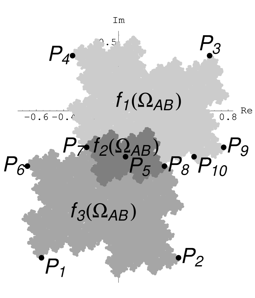
Figure 1. Components $f_{i}(\Omega_{AB})$ of the set $\Omega_{AB}$ and the points $P_{1},\ldots,P_{10}$ used in the proof of Proposition 2. $\Omega_{AB}$ is the union of the three shaded areas.

Point Coordinate $P_{1}$ $\frac{1}{2}\,(\beta^{2}-3\,\beta-1)$ $P_{2}$ $\frac{1}{2}\,(\beta^{2}-3\,\beta+1)$ $P_{3}$ $\frac{1}{2}\,(-\beta^{2}+\beta+1)$ $P_{4}$ $\frac{1}{2}\,(-\beta^{2}+\beta-1)$ $P_{5}$ $-\frac{1}{2}\,\beta$ $P_{6}$ $\frac{1}{2}\,(\beta^{2}-\beta-1)$ $P_{7}$ $\frac{1}{2}\,(-\beta^{2}-\beta-1)$ $P_{8}$ $\frac{1}{2}\,(\beta^{2}-\beta+1)$ $P_{9}$ $\frac{1}{2}\,(-\beta^{2}-\beta+1)$ $P_{10}$ $\frac{1}{2}\,(-\beta+1)$

Table 1. Coordinates of the points $P_{1},\ldots,P_{10}$ in Figure 1.

Proof.

To determine the boundary of $\Omega_{AB}$, we choose special points $P_{i}$ in $\Omega_{AB}$, see Figure 1 (for illustration) and Table 1 (for details). We first show how these points are determined. Demanding

$$P_{2}=f_{3}(P_{1}),\qquad P_{3}=f_{1}(P_{2}),\qquad P_{4}=f_{1}(P_{3}),\quad\text{and}\quad P_{1}=f_{3}(P_{4})$$

one gets the following fixed point equation

(15) $$P_{1}=f_{3}\circ f_{1}\circ f_{1}\circ f_{3}(P_{1})=\beta^{4}\,P_{1}+6\,\beta^{2}+2$$

for $P_{1}$, and similar results hold for $P_{2}$, $P_{3}$ and $P_{4}$. The unique solution of (15) is

$$P_{1}=\frac{1}{2}(\beta^{2}-3\,\beta-1).$$

Choosing

$$\begin{array}[]{lll}P_{5}=\frac{1}{2}(P_{1}+P_{3}),&P_{6}=f_{3}(P_{3}),&P_{7}=f_{1}(P_{4}),\\ P_{8}=f_{2}(P_{3}),&P_{9}=f_{1}(P_{1}),&P_{10}=\frac{1}{2}(P_{2}+P_{3})\end{array}$$

and setting $\tau$ to be the inversion in the center $P_{5}$ ($\tau:\,z\mapsto-z-\beta$) and $\kappa$ the one in the center $P_{10}$ ($\kappa:\,z\mapsto-z-\beta+1$), one can verify the following equations:

$$\begin{array}[]{lclclclcl}P_{1}&=&\tau(P_{3})\\ P_{2}&=&\tau(P_{4})&=&\kappa(P_{3})\\ P_{5}&=&\frac{1}{2}(P_{2}+P_{4})&=&\frac{1}{2}(P_{6}+P_{9})&=&\frac{1}{2}(P_{7}+P_{8})\\ P_{6}&=&\tau(P_{9})\\ P_{7}&=&f_{2}(P_{1})&=&f_{3}(P_{9})&=&\tau(P_{8})\\ P_{8}&=&f_{1}(P_{6})&=&f_{3}(P_{2})&=&\tau(P_{8})&=&\kappa(P_{9})\\ P_{10}&=&\frac{1}{2}(P_{8}+P_{9}).\end{array}$$

For the mappings, one finds

$$f_{1}\circ\tau=\tau\circ f_{3},\qquad f_{2}\circ\tau=\tau\circ f_{2}\quad\text{and}\quad f_{3}\circ\tau=\tau\circ f_{1},$$

showing that $\Omega_{AB}$ is inversion symmetric in the center $P_{5}$, i.e., $\tau(\Omega_{AB})=\Omega_{AB}$.

Denoting by $[P_{2},P_{3}]$ the “boundary” between $P_{2}$ and $P_{3}$ (the “right edge”), one finds

$$\begin{array}[]{lcl}[P_{2},P_{8}]&=&f_{3}\circ\tau\circ f_{1}([P_{2},P_{3}])\\[0.0pt] [P_{8},P_{9}]&=&f_{1}\circ\tau\circ f_{1}\circ\tau\circ f_{1}([P_{2},P_{3}])\\[0.0pt] [P_{9},P_{3}]&=&f_{1}\circ\tau\circ f_{1}([P_{2},P_{3}])\end{array}$$

and therefore the following IFS for $[P_{2},P_{3}]$:

(16) $$\begin{array}[]{lclclclcl}[P_{2},P_{3}]&=&g_{1}([P_{2},P_{3}])&\cup&g_{2}([P_{2},P_{3}])&\cup&g_{3}([P_{2},P_{3}]),\end{array}$$

where

(17) $$g_{1}(z)=-\beta^{2}\,z-\beta,\qquad g_{2}(z)=(2\beta^{2}+1)\,z+\beta^{2}+1,\quad\text{and}\quad g_{3}(z)=-\beta^{2}\,z-\beta^{2}.$$

Of course, we have not shown yet that $[P_{2},P_{3}]$ really is (a piece of) the boundary of $\Omega_{AB}$, so we just define $[P_{2},P_{3}]$ to be the unique compact solution of the IFS (16), which is inversion symmetric in the center $P_{10}$ because

$$g_{1}\circ\kappa=\kappa\circ g_{3},\qquad g_{2}\circ\kappa=\kappa\circ g_{2}\quad\text{and}\quad g_{3}\circ\kappa=\kappa\circ g_{1}.$$

Also, we know that $[P_{2},P_{3}]$ is connected since we can start the iteration with the straight line from $P_{2}$ to $P_{3}$. In each iteration, the image remains a (piecewise smooth) path from $P_{2}$ to $P_{3}$.

With the mappings $f_{1}$ and $\tau$, we get a boundary

$$\begin{array}[]{lclclclc}[P_{2},P_{3}]&\cup&f_{1}([P_{2},P_{3}])&\cup&\tau([P_{2},P_{3}]&\cup&\tau\circ f_{1}([P_{2},P_{3}])&=\\ [P_{2},P_{3}]&\cup&[P_{3},P_{4}]&\cup&[P_{4},P_{1}]&\cup&[P_{1},P_{2}]\end{array}$$

around a simply connected open set $U$ (we will prove in the next proposition that this boundary is non-self-intersecting). Now one can show that only the boundaries of $\overline{f_{i}(U)}$ intersect. Consider, for example, the region between $f_{2}(U)$ and $f_{3}(U)$. Then the boundary $[P_{7},P_{8}]$ on $f_{2}(U)$ is given by

$$\begin{array}[]{lclcl}[P_{7},P_{8}]&=&f_{2}\circ\tau\circ f_{1}([P_{2},P_{3}])&\cup&f_{2}([P_{2},P_{3}]),\end{array}$$

while the one on $f_{3}(U)$ is given by (taking orientation into account)

$$\begin{array}[]{lclcl}[P_{7},P_{8}]&=&f_{3}\circ\kappa\circ g_{2}([P_{2},P_{3}])&\cup&f_{3}\circ g_{3}([P_{2},P_{3}]).\end{array}$$

It is easy to verify that

$$f_{2}\circ\tau\circ f_{1}=f_{3}\circ\kappa\circ g_{2}\quad\text{and}\quad f_{2}=f_{3}\circ\kappa\circ g_{3}.$$

So the boundaries coincide. Similarly, one can check the region between $f_{1}(U)$ and $f_{2}(U)$ (note that $P_{7}$ and $P_{8}$ belong to all three sets $\overline{f_{i}(U)}$), and that the boundary of $U$ coincides with pieces of the boundaries of the $f_{i}(U)$ – so the situation is as expected from Figure 1. Therefore, the IFS is just touching. Also, we now know that $[P_{2},P_{3}]$ is really a piece of the boundary of $\Omega_{AB}$. ∎

Proposition 3.

Let $\Omega_{AB}$ be the unique compact solution of the IFS $(\ref{eq:IFS-AB})$. Then its boundary is non-self-intersecting.

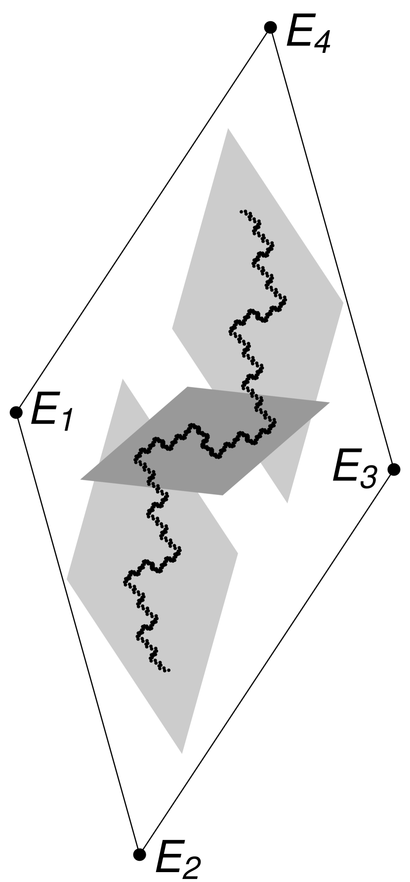
Figure 2. A rhombus $R$ with corners $E_{1},\ldots,E_{4}$, such that $g_{i}(R)\subset R$ for all $i$ (see (18)). The $g_{i}(R)$ are shaded in gray. For the coordinates of $E_{1},\ldots,E_{4}$, see Table 5.

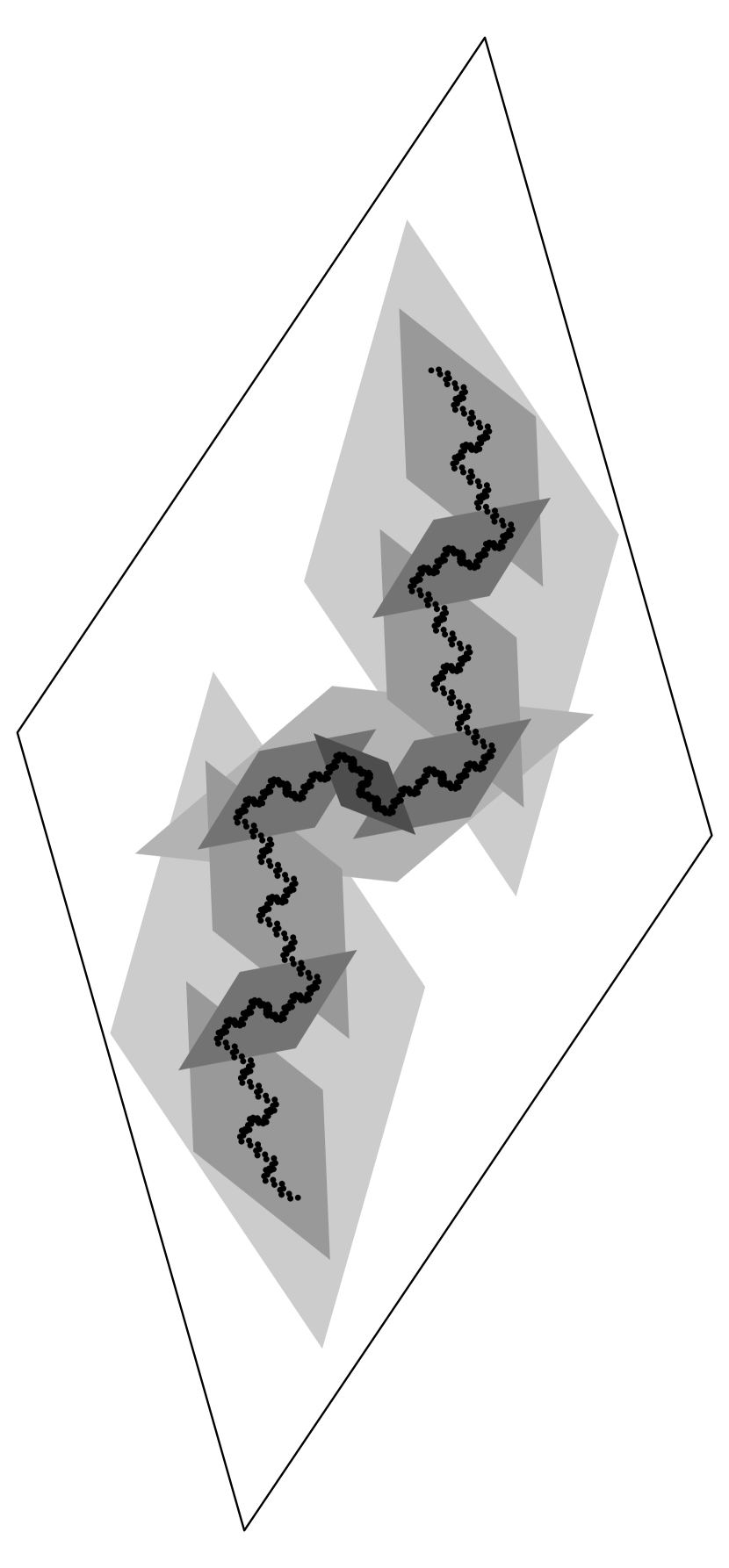
Figure 3. In addition to Figure 4, the second iteration of the rhombus $R$ is also shown, shaded in the dark gray. (20) is satisfied.

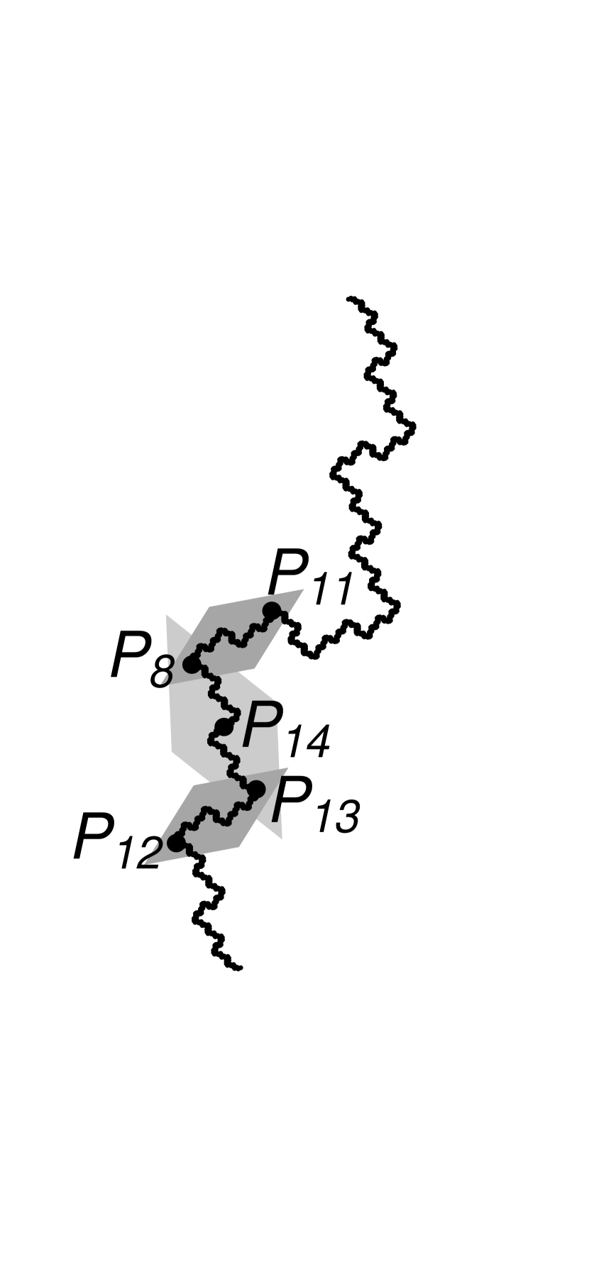
Figure 4. The situation around the “joint” $P_{8}$. We have an inversion symmetry in the center $P_{14}$. For the coordinates, see Table 5.

Proof.

We specify a (closed) rhombus $R$ (which surrounds the boundary $[P_{2},P_{3}]$ and the straight line from $P_{2}$ to $P_{3}$) such that its iteration in (12) will not leave $R$, i.e., such that

(18) $$\left(g_{1}(R)\cup g_{2}(R)\cup g_{3}(R)\right)\cap(\mathbb{R}^{2}\setminus R)=\varnothing.$$

Furthermore, we also require that

(19) $$g_{1}(R)\cap g_{3}(R)=\varnothing$$

and

(20) $$\begin{array}[]{ll}g_{1}(R)\cap g_{2}(g_{i}(R))=\varnothing&\mbox{for }i\neq 1\\ g_{2}(R)\cap g_{1}(g_{i}(R))=\varnothing&\mbox{for }i\neq 3\\ g_{2}(R)\cap g_{3}(g_{i}(R))=\varnothing&\mbox{for }i\neq 1\\ g_{3}(R)\cap g_{2}(g_{i}(R))=\varnothing&\mbox{for }i\neq 3.\end{array}$$

Such a rhombus $R$ exists, see Figure 4 for a picture of such a rhombus that satisfies the conditions of (18) and (19) and Table 5 for the coordinates of its corners (of course, we could also use a shape different from a rhombus). This rhombus also satisfies (20), see Figure 4.

Here, (19) tells us that $[P_{2},P_{8}]$ and $[P_{9},P_{3}]$ do not have a point in common; similar statements apply for (20). Each iterate of the rhombus is associated to a corresponding iterate of the boundary $[P_{2},P_{3}]$ or the straight line from $P_{2}$ to $P_{3}$ (denoted by $(P_{2},P_{3})$). We call two rhombi at the same iteration level neighbouring if their corresponding iteration of $(P_{2},P_{3})$ have a common endpoint. We see in Figure 4 that only neighbouring rhombi intersect at the second iteration level. We show that for any iteration level only neighbouring rhombi intersect.

We have verified the assertion for the first and second iteration level and proceed inductively. Since $g_{1}$, $g_{2}$ and $g{}_{3}$ are affine, we get the third iteration level as follows: The associated rhombi between $P_{2}$ and $P_{8}$ are a scaled down (by $g_{1}$) version of those of the second level, therefore the assertion holds for them. Similarly for the rhombi between $P_{8}$ and $P_{9}$ (by $g_{2}$) and between $P_{9}$ and $P_{3}$ (by $g_{3}$). So the only critical points remaining are the “joints” at $P_{8}$ and $P_{9}$. We show that at these points also only neighbouring rhombi intersect and for this, we make use of the self-similar structure of the boundary, see Figure 4: The boundary $[P_{12},P_{11}]$ is inversion symmetric in the center $P_{14}$. This is clear for $[P_{13},P_{8}]=g_{1}(g_{3}([P_{2},P_{3}]))$ (and therefore $P_{14}=g_{1}(g_{3}(P_{10}))$). But it also holds for $[P_{12},P_{13}]=g_{1}(g_{2}([P_{2},P_{3}]))$ and $[P_{8},P_{11}]=g_{2}(g_{1}(\kappa([P_{2},P_{3}])))$. So, since the assertion holds around $P_{13}$, it also holds around $P_{8}$ by symmetry. Similar arguments apply around $P_{9}$. So the assertion holds for the third iteration level, i.e., for the third iteration level only neighbouring rhombi intersect. But the same argument applies to all further iteration levels. So the assertion is true, i.e., for a given iteration level only neighbouring rhombi intersect. Also note that each rhombus has two neighbouring rhombi (with the exception of the “starting” and “ending” rhombi at $P_{2}$ and $P_{3}$ which only have one) and that there is no “rhombus loop”, i.e., going from $P_{2}$ to $P_{3}$ we cross each rhombus only once.

Now, suppose $[P_{2},P_{3}]$ is self-intersecting. Then there exist points $x,y\in[P_{2},P_{3}]$ ($x\neq y$) such that they are connected in $[P_{2},P_{3}]$ in two different ways, $W_{1}$ and $W_{2}$ (and we have a loop). We can choose points $u\in W_{1}$ and $v\in W_{2}$ such that $d(u,W_{2})=\min\{d(v,z)\mathbin{|}z\in W_{2}\}>0$ ($W_{2}\subset[P_{2},P_{3}]$ is compact) and $d(v,W_{1})>0$. But then, $u,v$ are in non-neighbouring rhombi for some iteration level $N$ (and then for all iteration levels $n\geq N$), since the length of a rhombus of the $N$th iteration level is at most $|\beta|^{2N}\cdot|E_{2}-E_{4}|$. So, we get a “rhombus loop” for this iteration level by the rhombi which overlay $W_{1}$ and $W_{2}$. This is a contradiction, therefore $[P_{2},P_{3}]$ is non-self-intersecting.

From this single edge we proceed to all of the boundary. Here, critical are the “joints” $P_{2}$, $P_{3}$, etc., again, because we get the other three parts by an affine map of this edge (e.g., $[P_{3},P_{4}]=f_{1}([P_{2},P_{3}])$) and opposite edges (i.e., $[P_{2},P_{3}]$ and $[P_{4},P_{1}]$) do not overlap, cf. Figure 5. But at $P_{2}$, an argument like the one at $P_{8}$ above applies, i.e., we have an inversion symmetry of part of the boundary in the center $\frac{1}{2}\,(P_{12}+P_{13})$ (and similar for the other “joints”). This extends our findings to the entire boundary. ∎

This also implies that the boundaries of $\Omega_{A}$, $\Omega_{B}$ and $\Omega_{C}$, respectively their union $\Omega$, are non-self-intersecting. Also, from the proof of the last proposition, we can deduce the following.

Corollary 1.

The point $0$ is an inner point of $f_{1}(\Omega_{AB})\subset\Omega_{A}$ and $-\beta$ is an inner point of $f_{3}(\Omega_{AB})\subset\Omega_{B}$.

Point Coordinate $E_{1}$ $P_{10}-i\,\frac{2}{5}\,(\beta^{2}-2\,\beta)$ $E_{2}$ $P_{2}+\frac{2}{5}\,(\beta^{2}-2\,\beta)$ $E_{3}$ $P_{10}+i\,\frac{2}{5}\,(\beta^{2}-2\,\beta)$ $E_{4}$ $P_{3}-\frac{2}{5}\,(\beta^{2}-2\,\beta)$ $P_{8}$ $\frac{1}{2}\,(\beta^{2}-\beta+1)$ $P_{11}$ $\frac{1}{2}\,(9\,\beta^{2}+\beta+5)$ $P_{12}$ $\frac{1}{2}\,(-3\,\beta^{2}-3\,\beta-1)$ $P_{13}$ $\frac{1}{2}\,(5\,\beta^{2}-\beta+3)$ $P_{14}$ $\frac{1}{2}\,(3\,\beta^{2}-\beta+2)$

Table 2. Coordinates of the points used in Figures 4 and 4.

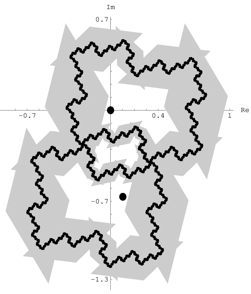
Figure 5. The points $0$ and $-\beta$ are represented as black dots. Also, the boundary is shown and the area of the rhombi (first iteration for all parts of the boundary) is shaded in gray. The boundary runs inside this shaded region, so $0$ and $-\beta$ are inner points.

Proof.

We again use the iteration of rhombi as in Proposition 3 to show that the two points are really inner points in the respective areas. For this, see Figure 5, where the first iteration of the rhombi is used for all parts of the boundary. Clearly, the points $0,-\beta$ are inner points, which can easily be checked by a simple (though somewhat tedious) calculation of distances. ∎

Proposition 4.

Let $\Omega_{AB}$ be the unique compact solution of the IFS $(\ref{eq:IFS-AB})$.

1. $\Omega_{AB}$ is inversion symmetric in the center $P_{5}=-\frac{1}{2}\beta$.

2. $\Omega_{AB}$ has Hausdorff dimension $h(\Omega_{AB})=2$.

3. $\Omega_{AB}$ has positive (Hausdorff and Lebesgue) measure (area).

4. The boundary $\partial\Omega_{AB}$ has vanishing (Lebesgue) measure.

5. There is a periodic tiling of the plane with $\Omega_{AB}$ as prototile.

Proof.

(i) See proof of Proposition 2.
(ii) Just touching implies the OSC, therefore $h(\Omega_{AB})=s(\Omega_{AB})=2$.
(iii) The OSC for $\Omega_{AB}$ (or any self-similar set with similarity dimension $s$) is equivalent to the positive Hausdorff measure condition $\mu^{s}(\Omega_{AB})>0$, where $\mu^{s}$ denotes the $s$-dimensional Hausdorff measure, see [8] and references therein. For Euclidean dimensions, Hausdorff and Lebesgue measure are connected by a nonzero multiplicative constant.
(iv) The similarity dimension $\tilde{s}=s(\partial\Omega_{AB})$ of the boundary is the solution of (contraction constants given in (17))

$$2\,|\beta|^{2\tilde{s}}+|\beta|^{3\tilde{s}}=1,$$

which is $\tilde{s}=-\log(\tau)/\log(|\beta|)\approx 1.22$ (where $\tau=\frac{1}{2}(1+\sqrt{5})$ is the golden ratio; the previous equation is solved by $|\beta|^{-\tilde{s}}=\tau$). Therefore, the statement follows from $h(\partial\Omega_{AB})\leq s(\partial\Omega_{AB})$.
(v) Because of the inversion symmetries $\tau$ of $\Omega_{AB}$ and $\kappa$ of $\partial\Omega_{AB}$ from $P_{2}$ to $P_{3}$ (see proof of Proposition 2), the “right edge” and the “left edge” differ only by a translation $P_{2}-P_{1}=1$, and, similarly, the “upper edge” and the “lower edge” differ by $P_{2}-P_{3}=\beta^{2}-2\,\beta$. ∎

Proposition 5.

Let $\Omega_{A},\,\Omega_{B},\,\Omega_{C}$ be the solution of the IFS $(\ref{eq:IFS})$, and $\Omega=\Omega_{A}\cup\Omega_{B}\cup\Omega_{C}$. Then $\Omega$ is a compact set, homeomorphic to a disc, with positive area. The boundary $\partial\Omega$ is a fractal of vanishing Lebesgue measure, which is non-self-intersecting. The set $\Omega$ admits a lattice tiling of $\mathbb{R}^{2}$, where the lattice is spanned by $P_{2}-P_{6}=-\beta+1$ and $P_{2}-P_{3}=\beta^{2}-2\,\beta$.

Proof.

It is clear from our construction that $\Omega$ is a compact set with simply connected interior. We have also seen that the boundary is connected and consists of finitely many pieces, each of which is obtained from a construction as used in the proof of Proposition 2. So, $\Omega$ must be homeomorphic to a disc. The remaining statements follow directly from Propositions 3 and 4, because the mappings in (14) are affine and the just touching property also holds for $\Omega=\Omega_{A}\cup\Omega_{B}\cup\Omega_{C}$. Since we also know the boundary of $\Omega$ (we have an IFS for every part of it), we can also verify the translation vectors by comparing the corresponding iterated function systems. Also, see Figure 6 for a depiction of these vectors. ∎

Corollary 2.

$\varLambda(\Omega)$ is a regular model set.∎

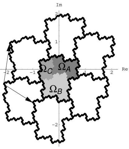
Figure 6. Components of the set $\Omega$, the periodic tiling of the plane ($\mathbb{C}$) with it and the corresponding translation vectors.

We can calculate the volume

(21) $$|\varGamma|=|\det(\boldsymbol{v}_{A},\boldsymbol{v}_{B},\boldsymbol{v}_{C})|=|\operatorname{Im}(\beta)|(3\,\alpha^{2}-4\,\alpha)=\frac{1}{2}\sqrt{59}\approx 3.84$$

of the fundamental domain of $\varGamma$. And because of the periodic tiling of the plane with $\Omega$ as a prototile, it is also easy to calculate the area $\mu_{\textnormal{int}}(\Omega)$ of $\Omega$: as $\mu_{\textnormal{int}}(\partial\Omega)=0$, $\mu_{\textnormal{int}}(\Omega)$ equals the area of a fundamental domain of the corresponding lattice of periods. This gives

(22) $$\mu_{\textnormal{int}}(\Omega)=|\det((P_{2}-P_{6}),(P_{2}-P_{3}))|=|\operatorname{Im}(\beta)|(\alpha^{2}-\alpha)=\frac{1}{2}\frac{1}{\sqrt{59}}(3\,\alpha^{2}-2\,\alpha+17)\approx 1.77.$$

Then the following lemma applies.

Lemma 1.

Let $\varGamma$ be a lattice in $\mathbb{R}\times\mathbb{R}^{m}$, $|\varGamma|$ be the volume of a measurable fundamental domain of $\varGamma$ in $\mathbb{R}\times\mathbb{R}^{m}$ with respect to the product $\mu\otimes\mu_{\textnormal{int}}$ of the Lebesgue measures $\mu$, $\mu_{\textnormal{int}}$ on $\mathbb{R}$, $\mathbb{R}^{m}$, respectively. Assume that we have a cut-and-project scheme like in $(\ref{eq:cutproj})$. If $\Omega$ is a bounded subset of $\mathbb{R}^{m}$ with almost no boundary, then the density $\operatorname{dens}(\varLambda(\Omega))$ of the corresponding regular model set in $\mathbb{R}$ is

$$\operatorname{dens}(\varLambda(\Omega))=\frac{\mu_{\textnormal{int}}(\Omega)}{|\varGamma|}.$$

Proof.

This follows from [28, Proposition 2.1] because the projection $\pi$ is one-to-one on $\varGamma$ by construction. ∎

With (6), (21) and (22), it is now easy to check that the density of the model set $\varLambda(\Omega)$ and the density of $\Sigma\textnormal{Kol}(3,1)$ are equal, i.e.,

(23) $$\frac{\mu_{\textnormal{int}}(\Omega)}{|\varGamma|}=\frac{1}{\ell}.$$

Proposition 6.

The sequence $\Sigma\textnormal{Kol}(3,1)$ is a subset of $\varLambda(\Omega)$. Further, they differ at most on positions of zero density and therefore have the same pure point diffraction spectrum.

Proof.

We choose $\boldsymbol{0},-\boldsymbol{v}_{B}\in\varGamma$. Then their projections into internal space are elements of the attractor $\Omega$, because $f_{1}(0)=0$ and $f_{3}(-\beta)=-\beta$. But starting with these two points, the iteration of the IFS in internal space just corresponds to the iteration in (3), respectively  (11), in physical space. Therefore, $\Sigma\textnormal{Kol}(3,1)\,\subset\,\varLambda(\Omega)$, because the star map of all iterates of $0$ and $-\alpha$ (i.e., $0$ and $-\beta$) stay in $\Omega$. Equation (23) shows that both sequences have the same density. So they can at most differ on positions of zero density.

Regular model sets have a pure point diffraction spectrum, see [9, 6, 29] and references therein. Therefore, the diffraction spectrum of $\varLambda(\Omega)$ is pure point, and $\Sigma\textnormal{Kol}(3,1)$, differing at most at positions of zero density, has the same spectrum by an argument in [18]. ∎

Theorem 1.

$\Sigma\textnormal{Kol}(3,1)$ is a regular model set (except possibly for positions of zero density) and has a pure point diffraction spectrum. Its autocorrelation is a norm almost periodic point measure, supported on a uniformly discrete subset of $\mathbb{Z}[\alpha]$.

Proof.

The first assertion follows from Proposition 6. The autocorrelation measure (see [18] for details) is supported on $\varLambda(\Omega)-\varLambda(\Omega)\subset\mathbb{Z}[\alpha]$. Since $\varLambda(\Omega)$ is a model set, it is also a Meyer set, hence $\varLambda(\Omega)-\varLambda(\Omega)$ is Delone. The norm almost periodicity follows from [6, Theorem 5]. ∎

What we have proved so far is enough to calculate the diffraction spectrum of $\Sigma\textnormal{Kol}(3,1)$ and Kol$(3,1)$, see Section 5. But in the next section, we want to show that $\varLambda(\Omega)$ really equals $\Sigma\textnormal{Kol}(3,1)$.

Remarks: For unimodular substitutions of Pisot type, i.e., Kol$(2m\pm 1,2m\mp 1)$ with $m\geq 1$, the procedure is essentially the same. Unfortunately, the IFS does not decouple like in (12) for $m>1$, which makes it technically more involved. For non-unimodular substitutions of Pisot type, the internal space is more complicated in having additional $p$-adic type components, see [30, 17, 7, 22, 23] for further details and examples.

The sequences $\Sigma\textnormal{Kol}(p,q)$, which are not of Pisot type, do not have a pure point spectral component outside $k=0$ by an argument in [10], see [31] for details.

Some of the results given have been studied extensively under the name of “Rauzy fractal”, e.g., that the windows have non-empty interior, that the windows do not overlap in this case (this follows from the so-called strong coincidence condition) and also the periodic tilability seems to follow from results in [1, 12, 35]. But we also need the lattice of the periodic tiling explicitly, as well as the induced IFS (16) for the boundary. Therefore, we opted to give an elementary and complete derivation here.

4. $\Sigma\textnormal{Kol}(3,1)$ is a generic model set

We set $\overset{\diamond}{\Omega}=\overset{\circ}{\Omega}_{A}\cup\overset{\circ}{\Omega}_{B}\cup\overset{\circ}{\Omega}_{C}\subset\Omega$ and $\partial\overset{\diamond}{\Omega}=\Omega\setminus\overset{\diamond}{\Omega}=\partial\Omega_{A}\cup\partial\Omega_{B}\cup\partial\Omega_{C}$. Then we can improve a statement of Proposition 6.

Proposition 7.

$\Sigma\textnormal{Kol}(3,1)$ is equal to the model set $\varLambda(\overset{\diamond}{\Omega})$.

Proof.

$\Sigma\textnormal{Kol}(3,1)\subset\varLambda(\overset{\diamond}{\Omega})$: Note that the mappings $f_{i}$ ($i\in\{0,1,3\}$) of (10’) are similarities (all directions are contracted by the same factor, here $|\beta|$). Therefore, they map balls around $x$ to balls around $f_{i}(x)$. Furthermore, they map balls in $\overset{\circ}{\Omega}_{k}$ to balls in $\overset{\circ}{\Omega}_{\ell}$ ($k,\ell\in\{A,B,C\}$). Since the starting points of the iteration (3) in internal space, namely $-\beta$ and $0$, are inner points of $\Omega_{B}$ and $\Omega_{A}$ by Corollary 1, one can also find balls of radius $\varepsilon>0$ around $-\beta$ and $0$ which lie entirely in $\overset{\circ}{\Omega}_{B}$ and $\overset{\circ}{\Omega}_{A}$, respectively. Since the iteration in physical space corresponds to the IFS in internal space, the star map of an arbitrary point in $\Sigma\textnormal{Kol}(3,1)$ is thus a point of $\overset{\diamond}{\Omega}$.
$\varLambda(\overset{\diamond}{\Omega})\subset\Sigma\textnormal{Kol}(3,1)$: Suppose $x\in\varLambda(\overset{\diamond}{\Omega})\setminus\Sigma\textnormal{Kol}(3,1)$. Then $x^{\star}$ and all its iterates of the IFS (10) are in $\overset{\diamond}{\Omega}$, by the same reasoning as before. Furthermore, the mappings $f_{i}$ ($i\in\{0,1,3\}$) are affine similarities and therefore all iterates of $x^{\star}$ are disjoint to all of the iterates of $-\beta$ and $0$. But then

$$\operatorname{dens}\Sigma\textnormal{Kol}(3,1)<\operatorname{dens}\varLambda(\overset{\diamond}{\Omega}),$$

because the set of iterates of $x$ under inflation has positive density in $\varLambda(\overset{\diamond}{\Omega})$. This contradicts Proposition 6. ∎

Note that not only the original sequence with $3$’s and $1$’s is inversion symmetric (see (4)), but also the positions in $\varLambda(\Omega_{AB})$.

Corollary 3.

$\varLambda(\Omega_{AB})$ is inversion symmetric in the center $-\frac{1}{2}\alpha$.

Proof.

The starting points $-\beta$ and $0$ and the IFS (12) are inversion symmetric in the center $P_{5}$. This corresponds, in physical space (by Galois conjugation), to inversion symmetry in the center $-\frac{1}{2}\alpha$. ∎

For the following, we need some more definitions, see [3] and [26]. If $\varLambda$ is a discrete point set in $\mathbb{R}^{d}$, we call $\mathcal{P}_{r}(u)$ an $r$-patch of a point $u\in\varLambda$, if $\mathcal{P}_{r}(u)=\varLambda\cap B_{r}(u)$, where $B_{r}(u)$ is the ball of radius $r$ about $u$. Often, we are only interested in the set of $\{\mathcal{P}_{r}(u)\mathbin{|}r>0,u\in\varLambda\}$ and an element of this set is simply called a patch. Two structures $\varLambda_{1}$ and $\varLambda_{2}$ are locally indistinguishable (or locally isomorphic or LI) if each patch of $\varLambda_{1}$ is, up to translation, also a patch of $\varLambda_{2}$ and vice versa. The corresponding equivalence class is called LI-class.

A discrete structure $\varLambda$ is repetitive, if for every $r>0$ there is a radius $R(r)>0$ such that within each ball of radius $R(r)$, no matter its position in $\mathbb{R}^{d}$, there is at least one translate of each $r$-patch. Note that every primitive substitution generates a repetitive sequence, wherefore $\Sigma\textnormal{Kol}(3,1)$ is repetitive.

We now look at generic model sets and show that $\varLambda(\Omega)$ is actually generic.

Lemma 2.

The set $C=\{c\in\mathbb{R}^{2}\mathbin{|}(c+\partial\overset{\diamond}{\Omega})\,\cap\,L^{\star}=\varnothing\}$ is dense in $\mathbb{R}^{2}$, especially $c+L^{\star}\subset C$ for $c\in C$.

Proof.

The set $C$ is not the empty set by Baire’s category theorem ($\partial\overset{\diamond}{\Omega}$ is a meager set, $L^{\star}$ is countable), by standard arguments, which in this context first appeared in [27, Section 2.2.2], also see [7]. But if $c\in C$, then $c+t\in C,\;\forall t\in L^{\star}$ (notice that $L^{\star}$ is an Abelian group), and $L^{\star}$ is dense. ∎

Proposition 8.

1. The model set $\varLambda(c+\Omega)$ is repetitive and generic for $c\in C$.

2. The model sets $\varLambda(c+\Omega)$ and $\varLambda(\tilde{c}+\Omega)$ are LI for $c,\tilde{c}\in C$.

3. $\Sigma\textnormal{Kol}(3,1)$ and $\varLambda(c+\Omega)$ are LI for $c\in C$.

Proof.

(i) The model set $\varLambda(c+\Omega)$ is generic by the definition of the set $C$. It is repetitive by [28, Theorem 6] and [29, Proposition 3.1].
(ii) This is a by now standard argument, apparently first used in [27, Lemma 2.1].
(iii) Since $\varLambda(c+\Omega)$ is repetitive, by [27, Lemma 1.2] it is enough to check that every patch of $\Sigma\textnormal{Kol}(3,1)$ also occurs as a patch of $\varLambda(c+\Omega)$: Let $\mathcal{P}$ be a patch of $\Sigma\textnormal{Kol}(3,1)$. Then $\mathcal{P}^{\star}\subset\overset{\diamond}{\Omega}$ by Proposition 7, and since $\mathcal{P}$ is a finite patch, we even know that there is an $\varepsilon>0$ such that $\mathcal{P}^{\star}\subset\overset{\diamond}{\Omega}_{\varepsilon}$, where $\overset{\diamond}{\Omega}_{\varepsilon}=\{t\in\mathbb{R}^{2}\mathbin{|}t\in\overset{\diamond}{\Omega},\,\operatorname{dist}(t,\partial\overset{\diamond}{\Omega})>\varepsilon\}$. The set $C$ is dense by Lemma 2, therefore there is a $\tilde{c}\in C$ such that $\mathcal{P}^{\star}\subset\tilde{c}+\Omega$. Then $\mathcal{P}\subset\varLambda(\tilde{c}+\Omega)$ and $\Sigma\textnormal{Kol}(3,1)$ and $\varLambda(\tilde{c}+\Omega)$ are LI. Since LI is an equivalence relation, it follows from (ii) that $\Sigma\textnormal{Kol}(3,1)$ and $\varLambda(c+\Omega)$ are LI for every $c\in C$. ∎

Proposition 9.

Define $C_{0}=\{c\in C\mathbin{|}0\in c+\Omega\}$. Then, for every $r>0$ and $c\in C_{0}$, we get

$$B_{r}(0)\cap\Sigma\textnormal{Kol}(3,1)=B_{r}(0)\cap\left(\varLambda(c+\Omega)+t\right)=B_{r}(0)\cap\varLambda(c+t^{\star}+\Omega)$$

for an appropriate $t\in\mathbb{Z}[\alpha]$. Additionally, it follows that $c+t^{\star}\in C_{0}$.

Proof.

By Proposition 8(iii) we know that $\varLambda(c+\Omega)$ and $\Sigma\textnormal{Kol}(3,1)$ are LI, therefore the patch $B_{r}(0)\cap\Sigma\textnormal{Kol}(3,1)$ occurs somewhere in $\varLambda(c+\Omega)$. By the choice of $C_{0}$, we can translate this patch in $\varLambda(c+\Omega)$ with $t\in\mathbb{Z}[\alpha]$ to the origin. In internal space, this is a translation $t^{\star}$ and by Lemma 2 we have $c+t^{\star}\in C$. But $\Sigma\textnormal{Kol}(3,1)$ has a point at the origin, so we even have $c+t^{\star}\in C_{0}$. ∎

Theorem 2.

$\Sigma\textnormal{Kol}(3,1)$ is a regular generic model set.

Proof.

Since $\Sigma\textnormal{Kol}(3,1)$ is the fixed point of a primitive substitution, it is repetitive, and the corresponding dynamical system is minimal, see [29, Proposition 3.1].

By Proposition 8(iii) the model set $\varLambda(c+\Omega)$ for $c\in C$ is in the LI-class of $\Sigma\textnormal{Kol}(3,1)$, hence the latter must be the limit of some sequence $(t_{i})_{i}$ of translations of $\varLambda(c+\Omega)$, where the translates $t_{i}$ can be restricted to elements of $\mathbb{Z}[\alpha]$ and $c+t_{i}\in C_{0}$ by Proposition 9.

However, if $\partial\Omega\cap L^{\star}\neq\varnothing$, there is a point $\tilde{x}\in\partial\overset{\diamond}{\Omega}\cap L^{\star}\cap\overset{\circ}{\Omega}$ with $\tilde{x}\in\partial\Omega_{A}\cap\partial\Omega_{B}$ (so $\tilde{x}$ lies on the common boundary of $\Omega_{A}$ and $\Omega_{B}$). This is because by appropriate combinations of the mappings $g_{1},g_{2},g_{3},\tau,\kappa,f_{0},f_{1},f_{2},f_{3},f_{4}$ and the translations by $P_{2}-P_{1},P_{2}-P_{3},P_{2}-P_{6}$ of Section 3, which all map $L^{\star}$ onto $L^{\star}$, we can “move” points on $\partial\overset{\diamond}{\Omega}$ from every “edge” to every other “edge”. We have $\varepsilon_{0}=\operatorname{dist}(\tilde{x},\partial\overset{\diamond}{\Omega}\setminus(\partial\Omega_{A}\cap\partial\Omega_{B}))>0$.

The inverse star image of this point must then be in any limit of sequences $\varLambda(t^{\star}_{i}+c+\Omega)$ with $c+t^{\star}_{i}\to 0$, but it is not in $\Sigma\textnormal{Kol}(3,1)$ — which is a contradiction. So no such point can exist and $\partial\Omega\cap L^{\star}=\varnothing$.

Regularity was established in Theorem 1 together with Proposition 7. ∎

This argument is rather general and applies in other situations as well. For a more elementary proof see the appendix.

Remark: By Proposition 5 we know that $\bigcup_{t\in G}(t+\Omega)=\mathbb{R}^{2}$, where $G=\langle-\beta+1,\,\beta^{2}-2\,\beta\rangle_{\mathbb{Z}}$ is a rank $2$ free Abelian group (a $2$-dimensional lattice) and by Theorem 2 that $L^{\star}=\mathbb{Z}[\beta]\,\subset\,\dot{\bigcup}_{t\in G}(t+\overset{\circ}{\Omega})$, where $\dot{\cup}$ denotes disjoint union. In physical space, we get

$$L=\mathbb{Z}[\alpha]=\dot{\bigcup_{s\in G^{\prime}}}(s+\Sigma\textnormal{Kol}(3,1)),$$

where

$$G^{\prime}=\langle-\alpha+1,\,\alpha^{2}-2\,\alpha\rangle_{\mathbb{Z}}=\langle\ell_{C}-\ell_{B},\,\ell_{A}-\ell_{B}\rangle_{\mathbb{Z}},$$

i.e., $\mathbb{Z}[\alpha]$ is the disjoint union of translates of the regular, generic model set $\Sigma\textnormal{Kol}(3,1)$. The set of translations needed is a rank $2$ subgroup, whose Galois dual in $\mathbb{Z}[\beta]$ is a lattice. But we can also write

$$L=\mathbb{Z}[\alpha]=\dot{\bigcup_{r\in\Sigma\textnormal{Kol}(3,1)}}(r+G^{\prime}),$$

so $L/G^{\prime}$ is a coset system with the structure of a model set. Now, let $\lambda(m)$ be the $m$-th element of $\Sigma\textnormal{Kol}(3,1)$ ($m\in\mathbb{Z}$). Then one can show that the induced group structure on this coset system is $(\lambda(m))+(\lambda(n))=(\lambda(m+n))$, i.e., it is the action of $\mathbb{Z}$ on $\Sigma\textnormal{Kol}(3,1)$. This group structure lines up with the deformation in the next section.

5. Deformation and Diffraction

In the cut-and-project scheme (7) with $H=\mathbb{R}^{m}$, let $\varphi:\mathbb{R}^{m}\to\mathbb{R}^{d}$ be a continuous function with compact support (e.g., $\Omega$). We call

$$\varLambda_{\varphi}(\Omega)=\{x+\varphi(x^{\star})\mathbin{|}x\in\varLambda(\Omega)\}$$

a deformed model set if it is also a Delone set, see [9]. The model set $\varLambda(\Omega)$ can be seen as deformed model set where the associated function $\varphi$ is trivial, i.e., $\varphi\equiv 0$. The diffraction spectrum of (deformed) model sets (where each of its points is represented by a normalized Dirac measure, say) can be calculated explicitly, see [9] for details. We write $\delta_{k}$ for the Dirac measure at $k$, i.e., $\delta_{k}(f)=f(k)$ for $f$ continuous. Also, we need the dual of a lattice $\varGamma\subset\mathbb{R}^{n}$ defined as

$$\varGamma^{\ast}:=\{y\in\mathbb{R}^{n}\mathbin{|}x.y\in\mathbb{Z},\,\forall x\in\varGamma\},$$

with $x.y$ denoting the Euclidean scalar product.

Proposition 10.

[9] Let $\varLambda_{\varphi}(\Omega)$ be a deformed model set in $\mathbb{R}^{d}$ constructed with a regular model set $\varLambda(\Omega)$ and a continuous function $\varphi$ of compact support. Then, the diffraction pattern of $\varLambda_{\varphi}(\Omega)$ is the positive pure point measure

$$\hat{\gamma}=\sum_{k\in\pi(\varGamma^{\ast})}|c_{k}(\varLambda_{\varphi}(\Omega))|^{2}\,\delta_{k},$$

where $\varGamma^{\ast}$ is the dual lattice of $\varGamma$, $\delta_{k}$ is the Dirac measure at $k$ and $c_{k}(\varLambda_{\varphi}(\Omega))$ is the Fourier-Bohr coefficient of $\varLambda_{\varphi}(\Omega)$ at $k$. This Fourier-Bohr coefficient exists and has the value

(24) $$c_{k}(\varLambda_{\varphi}(\Omega))=\left\{\begin{array}[]{cl}\frac{1}{|\varGamma|}\int_{\Omega}e^{-2\pi i\,(k.\varphi(y)-k^{\star}.y)}dy,&\text{if }(k,k^{\star})\in\varGamma^{\ast},\\ 0,&\text{otherwise.}\\ \end{array}\right.$$

∎

For a regular model set $\varLambda(\Omega)$ (where $\varphi\equiv 0$), the Fourier-Bohr coefficient is just given by the (inverse) Fourier transform of the characteristic function of the window $\Omega$.

For $\Sigma\textnormal{Kol}(3,1)$, we note that the support $F$ of the spectrum is dense in $\mathbb{R}$ since it is given by the $\mathbb{Z}$-span of the projection of the dual lattice vectors, i.e.,

(25) $$F=\mathbb{Z}\cdot\pi(\boldsymbol{v}^{\ast}_{A})+\mathbb{Z}\cdot\pi(\boldsymbol{v}^{\ast}_{B})+\mathbb{Z}\cdot\pi(\boldsymbol{v}^{\ast}_{C}),$$

but $\pi(\boldsymbol{v}^{\ast}_{B})=(\alpha-1)\,\pi(\boldsymbol{v}^{\ast}_{A})$ and therefore they are linearly independent over $\mathbb{Q}$.

To deform $\Sigma\textnormal{Kol}(3,1)$ to Kol$(3,1)$, we make the linear ansatz $\varphi(x^{\star})=a\,x^{\star}_{1}+b\,x^{\star}_{2}$, where $x^{\star}_{i}$ denotes the $i$th Cartesian component of the vector $x^{\star}\in\mathbb{R}^{2}$. With this $\varphi$, we now deform all bond lengths $\ell_{i}$ to the average bond length $\ell$, i.e., we have to solve the following linear system of equations ($i\in\{A,B,C\}$):

$$(\boldsymbol{v}_{i})_{1}+a\,(\boldsymbol{v}_{i})_{2}+b\,(\boldsymbol{v}_{i})_{3}=\ell.$$

This over-determined system is solved by

$$\begin{split}&a=\ell-1=\frac{1}{2}(-\alpha^{2}+\alpha+5)\approx 1.17\quad\text{and}\\ &b=\frac{\operatorname{Im}(\beta)}{59}\cdot(-\alpha^{2}-17\,\alpha+31)=\frac{1}{2\,\sqrt{59}^{3}}(-413\,\alpha^{2}+885\,\alpha-59)\approx-0.13.\end{split}$$

Due to the linearity of $\varphi$ (and the positivity of the bond lengths involved), this deformation does not alter the order of the points (i.e., for $x,x^{\prime}\in\varLambda(\Omega)$ with $x<x^{\prime}$, we always have $x+\varphi(x^{\star})<x^{\prime}+\varphi({x^{\prime}}^{\star})$). Note that the support $F$ of the spectrum stays the same as in (25), only the Fourier-Bohr coefficients change.

The positions in $\varLambda_{\varphi}(\Omega_{i})$ are now subsets of $\ell\cdot\mathbb{Z}$. To be more precise, we even have

$$\varLambda_{\varphi}(\Omega_{A})\cup\varLambda_{\varphi}(\Omega_{B})\cup\varLambda_{\varphi}(\Omega_{C})\,=\,\ell\cdot\mathbb{Z}.$$

Because of this embedding into $\ell\cdot\mathbb{Z}$, the diffraction spectrum of each of the aperiodic sets $\varLambda_{\varphi}(\Omega_{i})$ is $(\ell\cdot\mathbb{Z})^{\ast}$-periodic [2], i.e., it is periodic with period $1/\ell$ (note that $\mathbb{Z}^{\ast}=\mathbb{Z}$; the diffraction spectrum of $\Sigma\textnormal{Kol}(3,1)$ is not periodic). This might not be obvious from (24) at first sight, but for $n\in\mathbb{Z}$ we have (note that $\pi(\boldsymbol{v}^{\ast}_{i})=\rho_{i}/\ell$)

(26) $$\frac{n}{\ell}=n\,\pi(\boldsymbol{v}^{\ast}_{A}+\boldsymbol{v}^{\ast}_{B}+\boldsymbol{v}^{\ast}_{C})=\pi(n\,\boldsymbol{v}^{\ast}_{A}+n\,\boldsymbol{v}^{\ast}_{B}+n\,\boldsymbol{v}^{\ast}_{C}),$$

therefore, for every $k^{\prime}=k+\frac{n}{\ell}$ with $(k,k^{\star})\in\varGamma^{\ast}$, there is also a ${k^{\prime}}^{\star}$ with $(k^{\prime},{k^{\prime}}^{\star})\in\varGamma^{\ast}$ given by

$${k^{\prime}}^{\star}=k^{\star}+\pi_{\textnormal{int}}(n\,\boldsymbol{v}^{\ast}_{A}+n\,\boldsymbol{v}^{\ast}_{B}+n\,\boldsymbol{v}^{\ast}_{C}).$$

But with the chosen $\varphi$ we get

(27) $$(k^{\prime}-k).\varphi(y)-({k^{\prime}}^{\star}-k^{\star}).y\\ =n\,y_{1}\left[\frac{a}{\ell}-\left(\pi_{\textnormal{int}}(\boldsymbol{v}^{\ast}_{A}+\boldsymbol{v}^{\ast}_{B}+\boldsymbol{v}^{\ast}_{C})\right)_{1}\right]+n\,y_{2}\left[\frac{b}{\ell}-\left(\pi_{\textnormal{int}}(\boldsymbol{v}^{\ast}_{A}+\boldsymbol{v}^{\ast}_{B}+\boldsymbol{v}^{\ast}_{C})\right)_{2}\right]=0$$

because each of the terms in square brackets vanishes. Therefore

$$c_{k}(\varLambda_{\varphi}(\Omega_{i}))\,=\,c_{k^{\prime}}(\varLambda_{\varphi}(\Omega_{i}))$$

holds, and the spectrum is periodic with period $1/\ell$.

To obtain the diffraction spectrum of Kol$(3,1)$ from here, one only has to rescale the positions in $\varLambda_{\varphi}(\Omega)$ by a factor of $1/\ell$. To summarize:

Theorem 3.

The bi-infinite sequence Kol$(3,1)$, represented with equal bond lengths, is a deformed model set and has a pure point diffraction spectrum.∎

Remarks: By the same method, we can also find a deformation $\tilde{\varphi}(x^{\star})=\tilde{a}\,x^{\star}_{1}+\tilde{b}\,x^{\star}_{2}$ such that we represent the letter ‘$1$’ of Kol$(3,1)$ with an interval of length $\tilde{\ell}$ and the letter ‘$3$’ with one of length $3\,\tilde{\ell}$. For this, the letters $A,B,C$ have bond lengths $6\,\tilde{\ell},\,4\,\tilde{\ell},\,2\,\tilde{\ell}$, respectively. For the parameters of the deformation (the average bond length must be $\ell$ again), we get

$$\begin{split}&\tilde{\ell}=\frac{1}{4}\,(7\,\alpha^{2}-15\,\alpha+1)\approx 0.49,\qquad\tilde{a}=\frac{1}{2}\,(7\,\alpha^{2}-15\,\alpha-1)\approx-0.016\quad\text{and}\\ &\tilde{b}=\frac{\operatorname{Im}(\beta)}{59}\cdot(-179\,\alpha^{2}+379\,\alpha+3)=\frac{1}{2\,\sqrt{59}^{3}}(1239\,\alpha^{2}-767\,\alpha-4661)\approx-0.36.\end{split}$$

Now (26) changes to

$$\frac{n}{\tilde{\ell}}=\pi(6\,n\,\boldsymbol{v}^{\ast}_{A}+4\,n\,\boldsymbol{v}^{\ast}_{B}+2\,n\,\boldsymbol{v}^{\ast}_{C}),$$

and with the same calculation as before one gets an equation which corresponds to (27), where the two terms in square brackets

$$\left[\frac{\tilde{a}}{\tilde{\ell}}-\left(\pi_{\textnormal{int}}(6\,\boldsymbol{v}^{\ast}_{A}+4\,\boldsymbol{v}^{\ast}_{B}+2\,\boldsymbol{v}^{\ast}_{C})\right)_{1}\right]\quad\text{and}\quad\left[\frac{\tilde{b}}{\tilde{\ell}}-\left(\pi_{\textnormal{int}}(6\,\boldsymbol{v}^{\ast}_{A}+4\,\boldsymbol{v}^{\ast}_{B}+2\,\boldsymbol{v}^{\ast}_{C})\right)_{2}\right]$$

also both vanish. Therefore, the spectrum is periodic with period $1/\tilde{\ell}$ as expected [2], since $\varLambda_{\tilde{\varphi}}(\Omega)\subsetneqq\tilde{\ell}\cdot\mathbb{Z}$. This representation with integer bond lengths (after rescaling) has the advantage that the union of the three aperiodic sets $\varLambda_{\tilde{\varphi}}(\Omega_{i})$ is still an aperiodic set. Clearly, it is also pure point diffractive.

Kol$(3,1)$ in its natural setting with intervals of length $1$, or of lengths $3$ and $1$, can be obtained as a deformation of the model set $\Sigma\textnormal{Kol}(3,1)$ derived above, where the intervals have incommensurate length. The basic theory of this is fully developed in [9, 19], but one can also understand, from a dynamical systems point of view, which deformations are stable in the sense that they do not change the spectral type of the dynamical spectrum (and hence of the diffraction spectrum, due to unique ergodicity), see [4].

Appendix: An alternative proof of Theorem 2

By Proposition 9 we can choose a sequence $(c_{i})_{i}$ with $c_{i}=c+t^{\star}_{i}\in C_{0}$ ($t^{\star}_{i}\in L^{\star}$) such that $B_{r_{i}}\cap\Sigma\textnormal{Kol}(3,1)=B_{r_{i}}\cap\varLambda(c_{i}+\Omega)$ for every sequence $(r_{i})_{i}$ with $r_{i}>i$. Also, this statement holds for every subsequence $(c_{i_{j}})_{j}$.

Now, assume $\partial\overset{\diamond}{\Omega}\cap L^{\star}\neq\varnothing$. Then we have a point $\tilde{x}\in\partial\overset{\diamond}{\Omega}\cap L^{\star}\cap\overset{\circ}{\Omega}$ with $\tilde{x}\in\partial\Omega_{A}\cap\partial\Omega_{B}$. Set $\varepsilon_{0}=\operatorname{dist}(\tilde{x},\partial\overset{\diamond}{\Omega}\setminus(\partial\Omega_{A}\cap\partial\Omega_{B}))>0$. Then a translation $y\neq 0$ of $\Omega$ with $y\in B_{\varepsilon_{0}}(0)\cap C$ has the following effect: $\tilde{x}\in y+\overset{\diamond}{\Omega}$, because by the definition of $C$, $\tilde{x}$ cannot be on the boundary $y+\partial\overset{\diamond}{\Omega}$, and by the choice of $\varepsilon_{0}$, it must either be in $y+\Omega_{A}$ or $y+\Omega_{B}$.

Now take a sequence $(c_{i})_{i}$ as above. Clearly, this sequence must converge to $0$. Therefore, there is an $N$ such that $|c_{i}|<\varepsilon_{0}$ for all $i>N$. By choosing an appropriate subsequence $(c_{i_{j}})_{j}$ we get a sequence $(\tilde{c}_{j})_{j}$ with $\tilde{c}_{j}=c_{i_{j}}$ such that $\tilde{x}$ is always either in $\tilde{c}_{j}+\Omega_{A}$ or in $\tilde{c}_{j}+\Omega_{B}$. Also we have $B_{r_{i}}\cap\Sigma\textnormal{Kol}(3,1)=B_{r_{i}}\cap\varLambda(\tilde{c}_{i}+\Omega)$ for $r_{i}>i$. But both $\pi$ and $\pi_{\textnormal{int}}$ are one-to-one. Therefore, the inverse of the star map of $\tilde{x}$ must be a point of each $\varLambda(\tilde{c}_{i}+\Omega)$ and it also must be in $B_{R}(0)$ for some $R<\infty$. But by Proposition 7, it is not in $\Sigma\textnormal{Kol}(3,1)$. Therefore we get a contradiction and our assumption is wrong. So, $0\in C$ and $\Sigma\textnormal{Kol}(3,1)$ is generic by Proposition 8(i). ∎

References

- [1] P. Arnoux and S. Ito, “Pisot substitutions and Rauzy fractals”, Bull. Belg. Math. Soc. Simon Stevin 8 (2001), 181–207.
- [2] M. Baake, “Diffraction of weighted lattice subsets”, Canadian Math. Bulletin 45 (2002), 483–498; math.MG/0106111.
- [3] M. Baake, “A guide to mathematical quasicrystals”, in: Quasicrystals, eds. J.-B. Suck, M. Schreiber and P. Häussler, Springer, Berlin (2002), pp. 17–48; math-ph/9901014.
- [4] M. Baake and D. Lenz, “Deformation of Delone dynamical systems and topological conjugacy”; in preparation.
- [5] M. Baake and R.V. Moody, “Self-similar measures for quasicrystals”, in: Directions in Mathematical Quasicrystals, eds. M. Baake and R.V. Moody, AMS, Providence (2000), pp. 1–42; math.MG/0008063.
- [6] M. Baake and R.V. Moody, “Weighted Dirac combs with pure point diffraction”; preprint math.MG/0203030.
- [7] M. Baake, R.V. Moody and M. Schlottmann, “Limit-(quasi)periodic point sets as quasicrystals with -adic internal spaces”, J. Phys. A: Math. Gen. 31 (1998), 5755–5765; math-ph/9901008.
- [8] C. Bandt, “Self-similar tilings and patterns described by mappings”, in: The Mathematics of Long-Range Aperiodic Order, ed. R.V. Moody, Kluwer, Dordrecht (1997), pp. 45–83.
- [9] G. Bernuau and M. Duneau, “Fourier Analysis of deformed model sets”, in: Directions in Mathematical Quasicrystals, eds. M. Baake and R.V. Moody, AMS, Providence (2000), pp. 43–60.
- [10] E. Bombieri and J.E. Taylor, “Which distributions of matter diffract? An initial investigation”, J. Physique Coll. C3 (1986), 19–29.
- [11] S.I. Borewicz and I.R. Šafarevič, “Zahlentheorie”, Birkhäuser, Basel, 1966.
- [12] V. Canterini and A. Siegel, “Geometric representation of substitutions of Pisot type”, Trans. Amer. Math. Soc. 353 (2001), 5121–5144.
- [13] F.M. Dekking, “The spectrum of dynamical systems arising from substitutions of constant length”, Z. Wahrscheinlichkeitstheorie verw. Gebiete 41 (1978), 221–239.
- [14] F.M. Dekking, “Regularity and irregularity of sequences generated by automata”, Sém. Th. Nombres Bordeaux 1979–80, exposé 9, 901–910.
- [15] F.M. Dekking, “What is the long range order in the Kolakoski sequence?”, in: The Mathematics of Long-Range Aperiodic Order, ed. R.V. Moody, Kluwer, Dordrecht (1997), pp. 115–125.
- [16] G.A. Edgar, “Measure, Topology and Fractal Geometry”, Springer, New York, 1990.
- [17] F. Gähler and R. Klitzing, “The diffraction pattern of self-similar tilings”, in: The Mathematics of Long-Range Aperiodic Order, ed. R.V. Moody, Kluwer, Dordrecht (1997), pp. 141–174.
- [18] A. Hof, “On diffraction by aperiodic structures”, Commun. Math. Phys. 169 (1995), 25–43.
- [19] A. Hof, “Diffraction by aperiodic structures”, in: The Mathematics of Long-Range Aperiodic Order, ed. R.V. Moody, Kluwer, Dordrecht (1997), pp. 239–268.
- [20] J.E. Hutchinson, “Fractals and self-similarity”, Indiana Univ. Math. J. 30 (1981), 713–747.
- [21] W. Kolakoski, “Self generating runs, Problem 5304”, Amer. Math. Monthly 72 (1965), 674.
- [22] J.-Y. Lee and R.V. Moody, “Lattice substitution systems and model sets”, Discrete Comput. Geom. 25 (2001), 173–201; math.MG/0002019.
- [23] J.-Y. Lee, R.V. Moody and B. Solomyak, “Pure point dynamical and diffraction spectra”, Annales Henri Poincaré 3 (2002), 1003–1018; mp_arc/02-39.
- [24] J.M. Luck, C. Godrèche, A. Janner and T. Janssen, “The nature of the atomic surfaces of quasiperiodic self-similar structures”, J. Phys. A: Math. Gen. 26 (1993), 1951–1999.
- [25] R.V. Moody, “Meyer sets and their duals”, in: The Mathematics of Long-Range Aperiodic Order, ed. R.V. Moody, Kluwer, Dordrecht (1997), pp. 403–441.
- [26] R.V. Moody, “Model sets: a survey”, in: From Quasicrystals to More Complex Systems, eds. F. Axel, F. Dénoyer and J.P. Gazeau, EDP Sciences, Les Ulis, and Springer, Berlin (2000), pp. 145–166; math.MG/0002020.
- [27] M. Schlottmann, “Geometrische Eigenschaften quasiperiodischer Strukturen”, Dissertation, Universität Tübingen (1993).
- [28] M. Schlottmann, “Cut-and-project sets in locally compact Abelian groups”, in: Quasicrystals and Discrete Geometry, ed. J. Patera, AMS, Providence (1998), pp. 247–264.
- [29] M. Schlottmann, “Generalized model sets and dynamical systems”, in: Directions in Mathematical Quasicrystals, eds. M. Baake and R.V. Moody, AMS, Providence (2000), pp. 43–60.
- [30] A. Siegel, “Represéntation des systèmes dynamiques substitutifs non unimodulaires”, Ergodic Theory & Dynam. Systems, in press; preprint available from the author’s homepage101010 Presently at: http://www.irisa.fr/symbiose/people/siegel/Pro/publi.htm .
- [31] B. Sing, “Spektrale Eigenschaften der Kolakoski-Sequenzen”, Diploma Thesis, Universität Tübingen (2002); available from the author.
- [32] B. Sing, “Kolakoski- are limit-periodic model sets”, J. Math. Phys. 44 (2003), 899-912; math-ph/0207037.
- [33] V.F. Sirvent, “Modélos geométricos asociados a substituciones”, Habilitation (trabajo de ascenso), Universidad Simón Bolívar (1998); available from the author’s homepage111111 Presently at: http://www.ma.usb.ve/~vsirvent/publi.html .
- [34] V.F. Sirvent and B. Solomyak, “Pure discrete spectrum for one-dimensional substitutions of Pisot type”, Canadian Math. Bulletin 45 (2002), 697–710.
- [35] V.F. Sirvent and Y. Wang, “Self-affine tiling via substitution dynamical systems and Rauzy fractals”, Pacific J. Math. 206 (2002), 465–485.