Expansive Motions and the
Polytope of Pointed Pseudo-Triangulations

Abstract

We introduce the polytope of pointed pseudo-triangulations of a point set in the plane, defined as the polytope of infinitesimal expansive motions of the points subject to certain constraints on the increase of their distances. Its $1$-skeleton is the graph whose vertices are the pointed pseudo-triangulations of the point set and whose edges are flips of interior pseudo-triangulation edges.

For points in convex position we obtain a new realization of the associahedron, i.e., a geometric representation of the set of triangulations of an $n$-gon, or of the set of binary trees on $n$ vertices, or of many other combinatorial objects that are counted by the Catalan numbers. By considering the $1$-dimensional version of the polytope of constrained expansive motions we obtain a second distinct realization of the associahedron as a perturbation of the positive cell in a Coxeter arrangement.

Our methods produce as a by-product a new proof that every simple polygon or polygonal arc in the plane has expansive motions, a key step in the proofs of the Carpenter’s Rule Theorem by Connelly, Demaine and Rote (2000) and by Streinu (2000).

ω

1 Introduction

Polytopes for combinatorial objects.

Describing all instances of a combinatorial structure (e.g. trees or triangulations) as vertices of a polytope is often a step towards giving efficient optimization algorithms on those structures. It also leads to quick prototypes of enumeration algorithms using known vertex enumeration techniques and existing code [2, 9].

One particularly nice example is the associahedron, (see Figure 4 for an example): the vertices of this polytope correspond to Catalan structures. The Catalan structures refer to any of a great number of combinatorial objects which are counted by the Catalan numbers (see the extensive list in Stanley [24, ex. 6.19, p. 219]). Some of the most notable ones are the triangulations of a convex polygon, binary trees, the ways of evaluating a product of $n$ factors when multiplication is not associative (hence the name associahedron), and monotone lattice paths that go from one corner of a square to the opposite corner without crossing the diagonal.

In this paper we describe a new polyhedron whose vertices correspond to pointed pseudo-triangulations.

Pseudo-triangulations.

Pseudo-triangulations, as well as the closely related geodesic triangulations of simple polygons, have been used in Computational Geometry in applications such as visibility [18, 19, 20, 23], ray shooting [12], and kinetic data structures [1, 14]. The minimum or pointed pseudo-triangulations introduced in Streinu [25] have applications to non-colliding motion planning of planar robot arms. They also have very nice combinatorial and rigidity theoretic properties. The polytope we define in this paper adds to the former, and is constructed exploiting the latter.

Expansive motions.

An expansive motion on a set of points $P$ is an infinitesimal motion of the points such that no distance between them decreases.

Expansive motions were instrumental in the first proof of the Carpenter’s Rule Theorem by Connelly, Demaine and Rote [6]: Every simple polygon or polygonal arc in the plane can be unfolded into convex position without collisions. Streinu [25] built on this work, realizing the importance of pseudo-triangulations in connection with expansive motions and studying their rigidity properties. This paper provides a systematic study of expansive motions in one and two dimensions. The expansive motions of a set of $n$ points in the plane form a polyhedral cone of dimension $2n-3$ (the expansion cone). As by-products of our approach we get a new proof of the existence of expansive motions for non-convex polygons and polygonal arcs (Theorem 4.3) and a characterization of the extreme rays of the expansion cone of a planar point set in general position, as equivalence classes of pointed pseudo-triangulations with one convex hull edge removed, modulo rigid subcomponents (Proposition 2.8).

Our tool is the introduction of constrained expansions as expansive motions with a special lower bound on the edge length increase. They form a polyhedron obtained by translation of the facets of the expansion cone. Our main result is the following (see a more precise statement as Theorem 3.1):

Theorem.

Let $P$ be a set of $n$ points in general position in the plane, $b$ of them in the boundary of the convex hull. Then, there is a choice of constraints which produces as constrained expansions of $P$ a simple polyhedron of dimension $2n-3$ with a unique maximal bounded face of dimension $2n-b-3$ whose vertices correspond to pointed pseudo-triangulations and edges correspond to flips between them.

The flips mentioned in the statement are a certain neighborhood structure among pointed pseudo-triangulations (flips of interior edges). See the details in Section 2.

Two appearances of the associahedron.

For points in convex position, pseudo-triangulations coincide with triangulations. We prove (Corollary 5.5) that, in this case, our construction gives a polytope affinely equivalent to the standard $(n-3)$-dimensional associahedron obtained as a secondary polytope of the point set [28, Section 9.2]. Perhaps surprisingly, this shows that the secondary polytope of $n$ points in convex position in the plane (which lives in $\mathbb{R}^{n}$) can naturally be embedded as a face in a $(2n-3)$-dimensional unbounded polyhedron.

The associahedron appears again as the analog of our construction for points in one dimension (Section 5.3).

Rigidity.

The connection of these results with rigidity theory is also worth mentioning. Pointed pseudo-triangulations are special instances of infinitesimally minimally rigid frameworks in dimension $2$, whose combinatorial structure is well understood (see [13]). One-dimensional minimally rigid frameworks are trees, another well understood combinatorial structure. Adding the constraint of expansiveness is what leads to pointed pseudo-triangulations in $2$d, and to the special non-crossing and alternating trees which appear in Section 5.3.

Future perspectives.

It is our hope that the insight into one- and two-dimensional motions may eventually lead to generalizations to higher dimensions. There is no satisfactory definition of an analog of pseudo-triangulations in $3$ dimensions. The $3$-dimensional version of the robot arm motion planning problem, with potential applications to computational biology (protein folding), is much more challenging.

Overview.

In Section 2 we give the preliminary definitions and results. Section 3 contains the main result, the construction of the polytope of pointed pseudo-triangulations (ppt-polytope). Section 4 applies the main result to get a new proof for the existence of expansive motions for non-convex polygons and polygonal arcs in the plane. In Section 5 we present an alternative construction of the ppt-polytope and two special cases leading to the associahedron: points in convex position and the polytope of constrained expansions in dimension $1$. Section 6 attempts to put the results in 1 and 2 dimensions into a broader perspective, with the aim of extending the results to higher dimensions and to point sets which are not in general position. We conclude with some final comments in Section 7.

2 Preliminaries

Abbreviations and conventions.

Throughout this paper we will assume general position for our point sets, i.e. we assume that no $d+1$ points in $\mathbb{R}^{d}$ lie in the same hyperplane (unless otherwise specified). We abbreviate “polytope of pointed pseudo-triangulations” as ppt-polytope, “one-degree-of-freedom mechanism” as 1DOF mechanism and “pseudo-triangulation expansive mechanism” as pte-mechanism.

For an ordered sequence of $d+1$ points $q_{0},\dots,q_{d}\in\mathbb{R}^{d}$, $\det(q_{0},\dots,q_{d})$ denotes the determinant of the $(d+1)\times(d+1)$ matrix with columns $(q_{0},1),\dots,\allowbreak(q_{d},1)$. Equivalently, $\det(q_{0},\dots,q_{d})$ equals $d!$ times the Euclidean volume of the simplex with those $d+1$ vertices, with a sign depending on the orientation.

Pseudo-triangulations.

A pseudo-triangle is a simple polygon with only three convex vertices (called corners) joined by three inward convex polygonal chains, see Figure 1a. In particular, every triangle is a pseudo-triangle. A pseudo-triangulation is a partitioning of the convex hull of a point set $P=\{p_{1},\ldots,p_{n}\}$ into pseudo-triangles using $P$ as vertex set.

Pseudo-triangulations are graphs embedded on $P$, i.e. graphs drawn in the plane on the vertex set $P$ and with straight-line segments as edges. We will work with other graphs embedded in the plane. If edges intersect only at their end-points, as is the case for pseudo-triangulations, the graphs will be called non-crossing or plane graphs. A graph is pointed at a vertex $v$ if there is (locally) an angle at $v$ strictly larger than $\pi$ and containing no edges. Under our general position assumption, convex-hull vertices are pointed for any embedded graph, as are vertices of degree at most two. A graph is called pointed if it is pointed at every vertex. Parts (b) and (c) of Figure 1 (including the broken edges) show two pointed pseudo-triangulations of a certain point set.

Figure 1: (a) A pseudo-triangle. (b) A minimum, or pointed, pseudo-triangulation. (c) The broken edge in (b) is flipped, and gives another pointed pseudo-triangulation. (d) A schematic drawing of the flip operation. (e) The two edges involved in a flip may share a common vertex $p$.

The following properties of pseudo-triangulations were initially proved for the slightly different situation of pseudo-triangulations of convex objects by Pocchiola and Vegter [18, 19]. For completeness, we sketch the easy proofs (see also [3]).

Lemma 2.1.

(Streinu [25]) Let $P$ be a set of $n$ points in general position in the plane. Let $G$ be a pointed and non-crossing graph on $P$.

• $G$ has at most $2n-3$ edges, with equality if and only if it is a pseudo-triangulation.

• If $G$ is not a pseudo-triangulation, then edges can be added to it keeping it non-crossing and pointed.

Proof.

(a) If the graph $G$ is not connected, we can analyze the components separately. So let us assume that it is connected. Let $e$ and $f$ be the numbers of edges and bounded faces in $G$. Let $a^{+}$ and $a^{-}$ denote the number of angles which are $>\pi$ and $<\pi$, respectively. (By our general position assumption, there are no angles equal to $\pi$.) Clearly, $a^{+}+a^{-}=2e$. Pointedness means $a^{+}=n$ and, since any bounded face has at least three convex vertices, $a^{-}\geq 3f$ with equality if and only if $G$ is a pseudo-triangulation. The equation $2e\geq n+3f$, together with Euler’s formula $e=n+f-1$, implies $e\leq 2n-3$ (and $f\leq n-2$).

(b) The basic idea is that the addition of geodesic paths (i.e., paths which have shortest length among those sufficiently close to them) between convex vertices of a polygon keeps the graph pointed and non-crossing and, unless the polygon is a pseudo-triangle, there is always some of these geodesic paths going through its interior. ∎

Streinu [25] proved the following additional properties of pointed pseudo-triangulations, which we do not need for our results but which may interest the reader:

• Every pseudo-triangulation on $n$ points has at least $2n-3$ edges, with equality if and only if it is pointed. Hence, pointed pseudo-triangulations are the pseudo-triangulations with the minimum number of edges. For this reason they are called minimum pseudo-triangulations in [25]. In contrast with part (b) of Lemma 2.1, not every pseudo-triangulation contains a pointed one. An example of this is a regular pentagon with its central point, triangulated as a wheel. Hence, a minimal pseudo-triangulation is not always pointed.

• The graph of any pointed pseudo-triangulation has the Laman property: it has $2n-3$ edges and the subgraph induced on any $k$ vertices has at most $2k-3$ edges. This property characterizes generically minimally rigid graphs in the plane ([15], see also [13]); that is, graphs which are minimally rigid in almost all their embeddings in the plane.

• All pointed pseudo-triangulations can be obtained starting with a triangle and adding vertices one by one and adding or adjusting edges, in much the same way as the Henneberg construction of generically minimally rigid graphs (cf. [13, page 113]), suitably modified to give pointed pseudo-triangulations in intermediate steps (see the details in [25]).

The other crucial properties of pointed pseudo-triangulations that we use are that all interior edges can be flipped in a natural way (part (a) of the following statement) and that the graph of flips between pointed pseudo-triangulations of any point set is connected. Both results were known to Pocchiola and Vegter for pseudo-triangulations of convex objects (see [18, 19]). Parts (b) and (c) of Figure 1 show a flip between pointed pseudo-triangulations. An $O(n^{2})$ bound on the diameter of the flip graph is proved in [3].

Lemma 2.2.

(Flips between pointed pseudo-triangulations) Let $P$ be a point set in general position in the plane.

1. (Definition of Flips) When an interior edge (not on the convex hull) is removed from a pointed pseudo-triangulation of $P$, there is a unique way to put back another edge to obtain a different pointed pseudo-triangulation.

2. (Connectivity of the flip graph) The graph whose vertices are pointed pseudo-triangulations and whose edges correspond to flips of interior edges is connected.

Proof.

[3, 25] (a) When we remove an interior edge from a pointed pseudo-triangulation we get a planar and pointed graph with $2n-4$ edges. The same arguments of the proof of Lemma 2.1 imply now that $a^{-}=3f+1$. Hence, the new face created by the removal must be a pseudo-quadrilateral (that is, a simple polygon with exactly four convex vertices).

In any pseudo-quadrilateral there are exactly two ways of inserting an interior edge to divide it into pseudo-triangles, which can be obtained by the shortest paths between opposite convex vertices of the pseudo-quadrilateral (see the details in Lemma 2.1 of [26], and a schematic drawing in Figure 1d). One of these two is the edge we have removed, so only the other one remains. Note that the two interior edges of a pseudo-quadrilateral may be incident to the same vertex, see Figure 1e. This can only happen when the interior angle at this vertex is bigger than $\pi$.

(b) Let $p$ be a convex hull vertex in $P$. Pointed pseudo-triangulations in which $p$ is not incident to any interior edge are just pointed pseudo-triangulations of $P\setminus\{p\}$ together with the two tangent edges from $p$ to the convex hull of the rest. By induction, we assume all those pointed pseudo-triangulations to be connected to each other. To show that all others are also connected to those, just observe that if a pointed pseudo-triangulation has an interior edge incident to $p$, then a flip on that edge inserts an edge not incident to $p$. (The case of Figure 1e cannot happen for a hull vertex $p$.) Hence the number of interior edges incident to $p$ decreases. ∎

Infinitesimal rigidity.

In this paper we work mostly with points in dimensions $d=2$ and $d=1$. Occasionally we will use superscripts to denote the components of the vectors $p_{i}=(p_{i}^{1},\ldots,p_{i}^{d})$.

An infinitesimal motion on a point set $P=\{p_{1},\ldots,p_{n}\}\in\mathbb{R}^{d}$ is an assignment of a velocity vector $v_{i}=(v_{i}^{1},\ldots,v_{i}^{d})$ to each point $p_{i}$, $i=1,\ldots,n$. The trivial infinitesimal motions are those which come from (infinitesimal) rigid transformations of the whole ambient space. In $\mathbb{R}^{2}$ these are the translations (for which all the $v_{i}$’s are equal vectors) and rotations with a certain center $p_{0}$ (for which each $v_{i}$ is perpendicular and proportional to the segment $p_{0}p_{i}$). Trivial motions form a linear subspace of dimension $\binom{d+1}{2}$ in the linear space $(\mathbb{R}^{d})^{n}$ of all infinitesimal motions. Two infinitesimal motions whose difference is a trivial motion will be considered equivalent, leading to a reduced space of non-trivial infinitesimal motions of dimension $dn-\binom{d+1}{2}$. In particular, this is $n-1$ for $d=1$ and $2n-3$ for $d=2$. Rather than performing a formal quotient of vector spaces we will “tie the framework down” by fixing $\binom{d+1}{2}$ variables. E.g., for $d=1$ we can choose:

$$v_{1}=0$$ (1)

and for $d=2$ (assuming w.l.o.g. that $p_{2}^{2}\neq p_{1}^{2}$):

$$v_{1}^{1}=v_{1}^{2}=v_{2}^{1}=0$$ (2)

Here, $p_{1}$ and $p_{2}$ can be any two vertices. A different choice of normalizing conditions only amounts to a linear transformation in the space of infinitesimal motions.

In rigidity theory, a graph $G=(P,E)$ embedded on $P$ is customarily called a framework and denoted by $G(P)$. We will use the term framework when we want to emphasize its rigidity-theoretic properties (stresses, motions), but we will use the term graph when speaking about graph-theoretic properties, even if graph is embedded on a set $P$. For a given framework $G=(P,E)$, an infinitesimal motion such that $\langle p_{i}-p_{j},v_{i}-v_{j}\rangle=0$ for every edge $ij\in E$ is called a flex of $G$. This condition states that the length of the edge $ij$ remains unchanged, to first order. The trivial motions are the flexes of the complete graph, provided that the vertices span the whole space $\mathbb{R}^{d}$. A framework is infinitesimally rigid if it has no non-trivial flexes. It is infinitesimally flexible or an infinitesimal mechanism otherwise.

Infinitesimal motions are to be distinguished from global motions, which describe paths for each point throughout some time interval. In this paper we are not concerned with global motions, nor their associated concept of rigidity, weaker than infinitesimal rigidity ([7, Theorem 4.3.1] or [13, page 6]). Let us also insist that we distinguish between infinitesimal motions (of the point set) and flexes (of the framework or embedded graph), while the terms flex and infinitesimal motion are sometimes equivalent in the rigidity theory literature.

The (infinitesimal) rigidity map $M_{G(P)}\colon(\mathbb{R}^{d})^{n}\to\mathbb{R}^{E(G)}$ is a linear map associated with an embedded framework $G(P)$, $P\subset\mathbb{R}^{d}$. It sends each infinitesimal motion $(v_{1},\dots,v_{n})\in(\mathbb{R}^{d})^{n}$ to the vector of infinitesimal edge increases $(\langle p_{i}-p_{j},v_{i}-v_{j}\rangle)_{ij\in E}$. When no confusion arises, it will be simply denoted as $M$. The number $\langle p_{i}-p_{j},v_{i}-v_{j}\rangle$ is called the strain on the edge $ij$ in the engineering literature. As usual, the image of $M$ is denoted by $\operatorname{Im}M=\{\,f\mid f=Mv\,\}$. The matrix of $M$ is called the rigidity matrix. In this matrix, the row indexed by the edge $ij\in E$ has $0$ entries everywhere except in the $i$-th and $j$-th group of $d$ columns, where the entries are $p_{i}-p_{j}$ and $p_{j}-p_{i}$, respectively.

The kernel of $M$ (after reducing $\mathbb{R}^{dn}$ to $\mathbb{R}^{dn-\binom{d+1}{2}}$ by forgetting trivial motions) is the space of flexes of $G(P)$. In particular, a framework is infinitesimally rigid if and only if the kernel of its associated rigidity map $M$ is the subspace of trivial motions. In general, the dimension of the (reduced) space of flexes is the degree of freedom (DOF) of the framework. A 1DOF mechanism is a mechanism with one degree of freedom.

Finally, expansive (infinitesimal) motions $v_{1},\ldots,v_{n}$ are those which simultaneously increase (perhaps not strictly) all distances: $\langle p_{i}-p_{j},v_{i}-v_{j}\rangle\geq 0$ for every pair $i,j$ of vertices. A mechanism is expansive if it has non-trivial expansive flexes.

The following results of Streinu [25] can be obtained as a corollary of our main result (see the proof after the statement of Theorem 3.1).

Proposition 2.3.

(Rigidity of pointed pseudo-triangulations [25])

1. Pointed pseudo-triangulations are minimally infinitesimally rigid (and therefore rigid).

2. The removal of a convex hull edge from a pointed pseudo-triangulation yields a 1DOF expansive mechanism (called a pseudo-triangulation expansive mechanism or shortly a pte-mechanism). ∎

Part (a) is in accordance with the fact that the graph of any pointed pseudo-triangulation has the Laman property, and hence is generically rigid in the plane. It is a trivial consequence of (a) that the removal of an edge creates a (not necessarily expansive) 1DOF mechanism. The expansiveness of pte-mechanisms (part (b)) was proved in [25] using the Maxwell-Cremona correspondence between self-stresses and 3-d liftings of planar frameworks, a technique that was introduced in [6].

Self-stresses.

A self-stress (or an equilibrium stress) on a framework $G(P)$ (see [27] or [6, Section 3.1]) is an assignment of scalars $w_{ij}$ to edges such that $\forall i\in P$, $\sum_{ij\in E}w_{ij}(p_{i}-p_{j})=0$. That is, the self-stresses are the row dependences of the rigidity matrix $M$. The proof of the following lemma is then straightforward.

Lemma 2.4.

Self-stresses form the orthogonal complement of the linear subspace $\operatorname{Im}M\subset\mathbb{R}^{\binom{d}{2}}$. In other words, $(w_{ij})_{ij\in E}$ is a self-stress if and only if for every infinitesimal motion $(v_{1},\dots,v_{n})\in(\mathbb{R}^{d})^{n}$ the following identity holds:

$$\sum_{ij\in E}w_{ij}\langle p_{i}-p_{j},v_{i}-v_{j}\rangle=0\qed$$

As an example, the following result gives explicitly a stress for the complete graph on any affinely dependent point set:

Lemma 2.5.

Let $\sum_{i=1}^{n}\alpha_{i}p_{i}=0$, $\sum\alpha_{i}=0$, be an affine dependence on a point set $P=\{p_{1},\dots,p_{n}\}$. Then, $w_{ij}=\alpha_{i}\alpha_{j}$ for every $i,j$ defines a self-stress of the complete graph $G$ on $P$.

Proof.

For any $p_{i}\in P$ we have:

$$\sum_{ij\in G}w_{ij}(p_{i}-p_{j})=\sum_{j=1}^{n}\alpha_{i}\alpha_{j}(p_{i}-p_{j})=\alpha_{i}p_{i}\sum_{j=1}^{n}\alpha_{j}-\alpha_{i}\sum_{j=1}^{n}\alpha_{j}p_{j}=0.\qed$$

Let us analyze here the case of $d+2$ points $P=\{p_{1},\dots,p_{d+2}\}$ in general position in $\mathbb{R}^{d}$ (this is the first non-trivial case, because no self-stress can arise between affinely independent points). It can be easily checked that, under these assumptions, removing any single edge from the complete graph on $P$ leaves a minimally infinitesimally rigid graph. This implies that the complete graph has a unique self-stress (up to a scalar factor). This self-stress is the one given in Lemma 2.5 for the unique affine dependence on $P$. The coefficients of this dependence can be written as:

$$\alpha_{i}=(-1)^{i}\det([p_{1},\dots,p_{d+2}]\backslash\{p_{i}\}).$$

(Recall that $\det(q_{0},\dots,q_{d})$ is $d!$ times the signed volume of the simplex spanned by the $d+1$ points $q_{0},\dots,q_{d}\in\mathbb{R}^{d}$.)

The special case $d=2$, $n=4$ will be extremely relevant to our purposes, and it will be convenient to renormalize the unique self-stress as follows:

Lemma 2.6.

The following gives a self-stresses for any four points $p_{1},\dots,p_{4}$ in general position in the plane:

$$w_{ij}:=\frac{1}{\det(p_{i},p_{j},p_{k})\det(p_{i},p_{j},p_{l})}$$ (3)

where $k$ and $l$ are the two indices other than $i$ and $j$.

Proof.

Set $\alpha_{i}=(-1)^{i}\det([p_{1},\dots,p_{4}]\backslash\{p_{i}\})$ in Lemma 2.5 and divide all the $w_{ij}$’s of the resulting self-stress by the non-zero constant

$$-\det(p_{1},p_{2},p_{3})\det(p_{1},p_{2},p_{4})\det(p_{1},p_{3},p_{4})\det(p_{2},p_{3},p_{4}).\qed$$

The direct application of Lemma 2.5 would give as $w_{ij}$ a product of two determinants, rather than the inverse of such a product. The reason why we prefer the self-stress of Lemma 2.6 is because of the signs it produces. The reader can easily check, considering the two cases of four points in convex position and one point inside the triangle formed by the other three, that with the choice of Lemma 2.6 boundary edges always receive positive stress and interior edges negative stress. This uniformity is good for us because in both cases pointed pseudo-triangulations are the graphs obtained deleting from the complete graph any single interior edge.

The expansion cone.

We are given a set of $n$ points $P=(p_{1},\ldots,p_{n})$ in $\mathbb{R}^{d}$ that are to move with (unknown) velocities $v_{i}\in\mathbb{R}^{d}$, $i=1,\ldots,n$. An expansive motion is a motion in which no inter-point distance decreases. This is described by the system of homogeneous linear inequalities:

$$\langle p_{i}-p_{j},v_{j}-v_{i}\rangle\geq 0,\qquad\forall\ 1\leq i<j\leq n$$ (4)

and hence defines a polyhedral cone.

The only motions in the intersection of all facets of the cone are the trivial motions. Thus, when we add normalizing equations like (1) or (2), we get a pointed polyhedral cone containing the origin as a vertex. We call it the cone of expansive motions or simply the expansion cone of $P$.

An extreme ray of the expansion cone is given by a maximal set of inequalities satisfied with equality by non-trivial motions. Each inequality corresponds to an edge of the point set, so that the ray corresponds to a graph embedded in our point set. The cardinality of this set of edges is at least the dimension of the cone minus 1, but may be much larger. Let’s analyze the low dimensional cases.

For $d=1$ the expansion cone is not very interesting. Let’s assume that the points $p_{i}\in\mathbb{R}$ are labeled in increasing order $p_{1}<p_{2}<\cdots<p_{n}$. Then:

Proposition 2.7.

The expansion cone in one dimension has $n-1$ extreme rays corresponding to the motions where $p_{1},\ldots,p_{i}$ remain stationary and the points $p_{i+1},\ldots,p_{n}$ move away from them at uniform speed:

$$0=v_{1}=v_{2}=\cdots=v_{i}<v_{i+1}=\cdots=v_{n}$$ (5)

Proof.

Note that the actual values of $p_{i}$ are immaterial in this case. The expansion cone is given by the linear system $v_{j}\geq v_{i}$, $1\leq i\leq j\leq n$ plus the extra condition $v_{1}=0$, and any maximal set of inequalities satisfied with equality and yet not trivial is obviously given by (5). ∎

The $2$d case is more complex and requires additional terminology. 1DOF mechanisms may contain rigid subcomponents (r-components, cf. [13]): maximal sets of some $k$ vertices spanning a Laman subgraph on $2k-3$ edges. The r-components of pte-mechanisms are themselves pseudo-triangulations spanning convex subpolygons including all points in their interior. Adding edges to complete each r-component to a complete subgraph yields a collapsed pte-mechanism (see Figures 2 and 3).

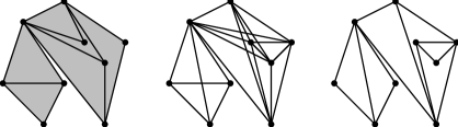
Figure 2: A pte-mechanism with rigid sub-components (convex subpolygons) drawn shaded, the corresponding collapsed pte-mechanism, and another pte-mechanism that yields the same expansive motion.

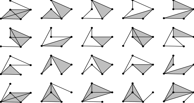
Figure 3: The collapsed pte-mechanisms corresponding to the 20 extreme rays of the expansion cone for a planar point set of $5$ points. The rigid sub-components (complete subgraphs) are shaded.

Proposition 2.8.

In dimension $2$, the extreme rays of the expansion cone correspond to the collapsed pte-mechanisms. ∎

The proof will be given in Section 4.1, after we have determined the extreme rays of a perturbed version of the polytope.

The polytope of constrained expansions.

The construction we will give in section 3 can roughly be interpreted as separating the pseudo-triangulations contained in the same collapsed pte-mechanisms, to obtain a polyhedron whose vertices correspond to distinct pseudo-triangulations. The original expansion cone is highly degenerate: its extreme rays contain information about all the bars whose length is unchanged by a motion of a 1DOF expansive mechanism. We would like to perturb the constraints (4) to eliminate these degeneracies and recover pure pseudo-triangulations. We do so by giving up homogeneity, i.e., by translating the facets of the expansion cone. Our system will become:

$$\langle v_{j}-v_{i},p_{i}-p_{j}\rangle\geq f_{ij},\qquad\ \forall 1\leq i<j\leq n$$ (6)

for some numbers $f_{ij}$. In some cases we will change these inequalities to equations for the edges on the convex hull of the given point set.

$$\langle v_{j}-v_{i},p_{i}-p_{j}\rangle=f_{ij},\qquad\ \text{for the convex hull edges $ij$}.$$ (7)

Section 3 proves our main result, Theorem 3.1: For any point set in general position in the plane and for some appropriate choices of the parameters $f_{ij}$, (6) defines a polyhedron whose vertices are in bijection with pointed pseudo-triangulations and all lie in a unique maximal bounded face given by (7). We call this face the “polytope of pointed pseudo-triangulations” or ppt-polytope.

A similar thing in 1d is done in Section 5.3, with the surprising outcome that the (unique) maximal bounded face of the polyhedron turns out to be an associahedron with vertices corresponding to non-crossing alternating trees (which are Catalan structures, as shown in [10]). The next paragraph prepares the ground for this result.

The associahedron.

The associahedron is a polytope which has a vertex for every triangulation of a convex $n$-gon, and in which two vertices are connected by an edge of the polytope if the two triangulations are connected by an edge flip. Equivalently, various types of Catalan structures are reflected in the associahedron. Fig. 4 shows an example.

Figure 4: The three-dimensional associahedron. The vertices represent all triangulations of a convex hexagon or all possible ways to insert parentheses into the product $a*b*c*d*e$. Left: a symmetric representation, the secondary polytope of a regular hexagon. Right: our representation, from Section 5.3. Both pictures are orthogonal projections.

There is an easy geometric realization of this polytope associated with each set $P$ of $n$ points in convex position in the plane, as a special case of a secondary polytope (Gel^′fand, Zelevinskiǐ, and Kapranov [11], see also Ziegler [28, Section 9.2]). Every triangulation is represented by a vector $(a_{1},\ldots,a_{n})$ of $n$ component with the entry $a_{i}$ being simply the sum of the areas of all triangles of the triangulation that are incident to the $i$-th vertex. We will refer to this realization as the classical realization of the associahedron. It depends on the location of the vertices of the convex $n$-gon, but all polytopes that one gets in this way are combinatorially equivalent. Their face lattice is the poset of polygonal subdivisions of the $n$-gon or, in the terminology of the previous paragraphs, non-crossing and pointed graphs embedded in $P$ and containing the $n$ convex hull edges. But observe that the word “pointed” is superfluous for a graph with vertices in convex position. The order structure in this poset is just inclusion of edge sets (in reverse order since maximal graphs represent vertices).

Dantzig, Hoffman, and Hu [8, Section 2], and independently de Loera et al. [17] in a more general setting, have given other representations of the set of triangulations as the vertices of a 0-1-polytope in $\binom{n}{3}$ variables corresponding to the possible triangles of a triangulation (the universal polytope), or in $\binom{n}{2}$ variables corresponding to the possible edges of a triangulation. These realizations are in a sense most natural, but they have higher dimensions and have more adjacencies between vertices than the associahedron. Every classical associahedron, however, arises as a projection of the universal polytope. The first published realization of an associahedron is due to Lee [16], but it is not fully explicit. A few earlier and more complicated ad-hoc realizations that were never published are mentioned in Ziegler [28, Section 0.10].

In this paper the associahedron appears in two forms. First, we will show that for $n$ points in convex position our polytope of pointed pseudo-triangulations is affinely equivalent to the secondary polytope of the configuration, which is a classical associahedron (Section 5.2). Second, as mentioned before, our construction adapted to a one-dimensional point configuration produces in a natural way an associahedron (Section 5.3). Notice that in dimension $1$ the coordinates $p_{i}$ can be eliminated from the constraints (6). Only the order of points along the line matters. One can also look at the whole arrangement of hyperplanes of the form

$$v_{j}-v_{i}=g_{ij}.$$

This arrangement, for various special values of $g$, has been the object of extensive combinatorial studies. For $g\equiv 0$ it is the classical Coxeter or reflection arrangement of type $A_{n}$. The case $g\equiv 1$ has been studied by Postnikov and Stanley [22]. The expansion cone of a 1d point set is the positive cell in the arrangement $A_{n}$, and our associahedron is a bounded face of the polyhedron obtained by translating the facets of this cell.

A different realization of the associahedron based in the root system of type $A_{n}$ has recently appeared in [5]. It is interesting that these two new associahedra are not affinely equivalent to any classical associahedron obtained as a secondary polytope, or to one another. Also, that we are trying to get a simple polyhedron, in contrast to the above-mentioned choices of $g$ which lead to highly degenerate arrangements.

3 The Main Result: the Polytope of Pointed Pseudo-Triangulations

In this section we prove our main result.

Theorem 3.1.

For every set $P=\{p_{1},\dots,p_{n}\}$ of $n\geq 3$ planar points in general position, there is a choice of $f_{ij}$’s for which equations (6) together with the normalizing equations (2) define a simple polyhedron $\bar{X}_{f}(P)$ of dimension $2n-3$ with the following properties:

1. The face poset of the polyhedron equals the opposite of the poset of pointed and non-crossing graphs on $P$, by the map sending each face to the set of edges whose corresponding equations (6) are satisfied with equality over that face. In particular:

   1. Vertices of the polyhedron are in 1-to-1 correspondence with pointed pseudo-triangulations of $P$.

   2. Bounded edges correspond to flips of interior edges in pseudo-triangulations, i.e., to pseudo-triangulations with one interior edge removed.

   3. Extreme rays correspond to pseudo-triangulations with one convex hull edge removed.

2. The face $X_{f}(P)$ obtained by changing to equalities (7) those inequalities from (6) which correspond to convex hull edges of $P$ is bounded (hence a polytope) and contains all vertices. In other words, it is the unique maximal bounded face, and its 1-skeleton is the graph of flips among pointed pseudo-triangulations.

The proof is a consequence of lemmas proved throughout this section. Theorem 3.9 states that the choice $f_{ij}:=\det(a,p_{i},p_{j})\det(b,p_{i},p_{j})$ produces the desired object, where $a$ and $b$ are any fixed points in the plane. In Section 5.1 we will derive a more canonical description of the polyhedron (and the polytope) in question.

It turns out that the polyhedron $\bar{X}_{f}(P)$ is the most convenient object for the proof. The properties of the polytope $X_{f}(P)$ (part 2 of the theorem) and the extreme ray description of the expansion cone (Proposition 2.8), which may be more interesting by themselves, are then easily derived.

Before going on, let us see that Theorem 3.1 implies Proposition 2.3. Observe that a framework is minimally infinitesimally rigid if and only if the hyperplanes $\langle p_{i}-p_{j},v_{i}-v_{j}\rangle=0$ corresponding to its edges $ij$ meet transversally and at a single point, in the $(2n-3)$-dimensional space given by equations (2). Part 1.a of our theorem says that this happens for the $2n-3$ translated hyperplanes $\langle p_{i}-p_{j},v_{i}-v_{j}\rangle=f_{ij}$ corresponding to any pointed pseudo-triangulation, hence giving part (a) of Proposition 2.3. An (infinitesimally) expansive 1DOF mechanism is one whose corresponding hyperplanes intersect in a line contained in the expansion cone. Part 1.c of the theorem says that this happens for a pointed pseudo-triangulation with one hull edge removed, giving part (b) of Proposition 2.3.

The polyhedron and the polytope of constrained expansions.

The solution set $v\in{(\mathbb{R}^{2})}^{n}$ of the system of inequalities (6) together with the normalizing equations (2) will be called the polyhedron of constrained expansions $\bar{X}_{f}(P)$ for the set of points $P$ and perturbation parameters (constraints) $f$. We will frequently omit the point set $P$ when it is clear from the context. A solution $v$ may satisfy some of the inequalities in (6) with equality: the corresponding edges $E(v)$ of $G$ are said to be tight for that solution. In the same way, for a face $K$ of $\bar{X}_{f}$ we call tight edges of $K$ and denote $E(K)$ the edges whose equations are satisfied with equality over $K$ (equivalently, over a relative interior point of $K$). This is the correspondence that Theorem 3.1 refers to: the edges $E(K)$ of a face $K$ form the pointed and non-crossing graph corresponding to that face.

When $f\equiv 0$, we just get the expansion cone $\bar{X}_{0}$ itself (in this sense, our notations $\bar{X}_{0}$ and $\bar{X}_{f}$ are consistent.) This cone equals the recession cone of $\bar{X}_{f}$, for any choice of $f$. (The recession cone of a polyhedron is the cone of vectors parallel to infinite rays contained in the polyhedron.) We will first establish a few properties of the expansion cone.

Lemma 3.2.

1. The expansion cone $\bar{X}_{0}$ is a pointed polyhedral cone of full dimension $2n-3$ in the subspace defined by the three equations (2). (In this context, “pointed” means that the origin is a vertex of the cone.)

2. Consider the set $E(v)$ of tight edges for any feasible point $v\in\bar{X}_{0}$. If $E(v)$ contains

   1. two crossing edges,

   2. a set of edges incident to a common vertex with no angle larger than $\pi$ (witnessing that $E(v)$ is not pointed at this vertex), or

   3. a convex subpolygon,

   then $E(v)$ must contain the complete graph between the endpoints of all involved edges. In case (iii), this complete graph also includes all points inside the convex subpolygon.

Proof.

(a) The dilation (scaling motion) $v_{i}:=p_{i}$ satisfies all inequalities (4) strictly. By adding a suitable rigid motion, the three equations (2) can be satisfied, too, without changing the status of the inequalities (4), and so we get a relative interior point in the $(2n-3)$-dimensional subspace (2).

If the cone were not pointed, it would contain two opposite vectors $v$ and $-v$. From this we would conclude that $\langle v_{j}-v_{i},p_{j}-p_{i}\rangle=0$ for all $i,j$, and hence $v$ would be a flex of the complete graph on $P$. By the normalizing equations (2), $v$ must then be $0$.

(b) We first consider (iii), which is the most involved case. Let $v$ be an expansive motion which preserves all edge lengths of some convex polygon. First we see that $v$ preserves all distances between polygon vertices: indeed, if it preserves lengths of polygon edges but is not a trivial motion of the polygon then the angle at some polygon vertex $p_{i}$ infinitesimally decreases, because the sum of angles remains constant. But decreasing the angle at $p_{i}$ while preserving the lengths of the two incident edges implies that the distance between the two vertices adjacent to $p_{i}$ in the polygon decreases. This is a contradiction.

By choosing $p_{1}$ and $p_{2}$ in (2) to be polygon vertices, the above implies that the polygon remains stationary under $v$. Now no interior point $p_{i}$ can move with respect to the polygon, without decreasing the distance to some polygon vertex: If $v_{i}\neq 0$, there is at least one hull vertex $p_{j}$ in the half-plane $\langle p_{i}-p_{j},v_{i}\rangle<0$. The edge $ij$ will then violate condition (4).

Case (ii) is similar: If the edges incident to a vertex $p_{i}$ do not move rigidly, at least one angle between two neighboring edges must decrease, and, this angle being less than $\pi$, this implies that the distance between the endpoints of these edges decreases, a contradiction.

For case (i), we apply Lemma 2.4 to our given four-point set in convex position, with the self-stress of Lemma 2.6, which is positive for the four hull edges and negative for the two diagonals. This implies that this four-point set can have no non-trivial expansive motion which is not strictly expansive on at least one of the two diagonals. ∎

As an immediate consequence of Lemma 3.2(a), we get:

Corollary 3.3.

$\bar{X}_{f}(P)$ is a $(2n-3)$-dimensional unbounded polyhedron with at least one vertex, for any choice of parameters $f$. ∎

It is easy to derive part 2 of Theorem 3.1 from part 1. For every vertex or bounded edge of $\bar{X}_{f}(P)$, the set $E(v)$ contains all convex hull edges of $P$. On the contrary, for any unbounded edge (ray) of $\bar{X}_{f}(P)$, the set $E(v)$ misses some convex hull edge of $P$. Hence, by setting to equalities the inequalities corresponding to convex hull edges we get a face $X_{f}(P)$ of $\bar{X}_{f}(P)$ which contains all vertices and bounded edges of $\bar{X}_{f}(P)$, but no unbounded edge.

In order to prove part 1, we first need to check that indeed $X_{f}$ is a bounded face, and hence a polytope which we call the polytope of constrained expansions or pce-polytope for the set of points $P$ and perturbation parameters $f$.

Lemma 3.4.

For any choice of $f$, $X_{f}(P)$ is a bounded set.

Proof.

Suppose that $v_{0}+tv$ is in $X_{f}$ for all $t\geq 0$. Then we must have $v\in X_{0}$. Hence, it suffices to show that $X_{0}=0$, i.e. that the framework consisting of all convex hull edges has no non-trivial expansive flexes. This is an immediate consequence of Lemma 3.2b(iii). ∎

Reducing the problem to four points.

We call a choice of the constants $f=(f_{ij})\in\mathbb{R}^{\binom{n}{2}}$ valid if the corresponding polyhedron $\bar{X}_{f}$ of constrained expansions has the combinatorial structure claimed in Theorem 3.1.

Lemma 3.5.

A choice of $f\in\mathbb{R}^{\binom{n}{2}}$ is valid if and only if the graph $E(v)$ of tight edges corresponding to any feasible point $v\in\bar{X}_{f}(P)$ is non-crossing and pointed.

Proof.

Necessity is trivial, by definition of being valid. To see sufficiency note that, by Corollary 3.3, $\bar{X}_{f}$ has dimension $2n-3$. Thus, any vertex $v$ of the polyhedron is incident to at least $2n-3$ faces $E(v)$. If $E(v)$ is non-crossing and pointed, Lemma 2.1 implies that $E(v)$ has exactly $2n-3$ incident faces and is a pointed pseudo-triangulation. In particular, the polyhedron is simple. Also, since the tight edges of faces incident to $v$ are different subgraphs of $E(v)$, the poset of faces incident to the vertex $v$ is the poset of all subgraphs of the pointed pseudo-triangulation $E(v)$.

It remains only to show that every pointed pseudo-triangulation actually appears as a vertex, for which we use a somewhat indirect argument, based on the fact that the flip graph is connected. This type of argument has also been used by Carl Lee for the case of the associahedron in [16], where it is attributed to Gil Kalai and Micha Perles.

Since the polytope is simple, every vertex $v$ is incident to $2n-3$ edges of $\bar{X}_{f}$. The sets of tight edges corresponding to them are the $2n-3$ subgraphs of $E(v)$ obtained removing a single edge. We denote by $K_{ij}$ the polyhedral edge corresponding to the removal of $ij$. By Lemma 3.4, if $ij$ is interior then $K_{ij}$ is bounded. Hence, it is incident to another vertex, which must correspond to a pointed pseudo-triangulation that completes $E(v)-\{ij\}$. By Lemma 2.2(a), this can only be the one obtained from $E(v)$ by a flip at $ij$. Together with the fact that the flip graph is connected (Lemma 2.2(b)) and that $\bar{X}_{f}$ has at least one vertex, this implies that all pointed pseudo-triangulations appear as vertices of $\bar{X}_{f}$, and hence that all pointed and non-crossing graphs appear as well.

Also, the extreme rays have the structure predicted in Theorem 3.1. For a convex hull edge $ij$, $K_{ij}$ must be an unbounded edge because there is no other pointed pseudo-triangulation that contains $E(v)-\{ij\}$. ∎

We now conclude that valid perturbation vectors $f\in\mathbb{R}^{\binom{n}{2}}$ can be recognized by looking at $4$-point subsets only.

Lemma 3.6.

A choice of $f\in\mathbb{R}^{\binom{n}{2}}$ is valid if and only if it is valid when restricted to every four points of $P$.

Proof.

By the previous Lemma, if $f$ is not valid for $P$ then there is a point $v$ of $\bar{X}_{f}$ for which the graph $E(v)$ is either non-pointed or crossing. In either case, there is a subset of four points $P^{\prime}\subseteq P$ on which the induced subgraph is non-pointed or crossing. Let $v^{\prime}$ and $f^{\prime}$ denote $v$ and $f$ restricted to $P^{\prime}$. Then, $v^{\prime}$ is in $\bar{X}_{f^{\prime}}(P^{\prime})$ and the graph $E(v^{\prime})$ is crossing or not pointed, hence $f^{\prime}$ is not valid on $P^{\prime}$. Contradiction. ∎

The case of four points.

Theorem 3.7.

A choice of perturbation parameters $f\in\mathbb{R}^{\binom{4}{2}}$ on four points $P=(p_{1},p_{2},p_{3},p_{4})$ forms a valid choice if and only if

$$\sum_{1\leq i<j\leq 4}w_{ij}f_{ij}>0,$$ (8)

where the $w_{ij}$’s are the unique self-stress on the four points, with signs chosen as in Lemma 2.6.

For a set of four points $P=(p_{1},p_{2},p_{3},p_{4})$, we denote by $G_{ij}$ the graph on $P$ whose only missing edge is $ij$. Recall that the choice of self-stress on four points has the property that $G_{ij}$ is pointed and non-crossing (equivalently, $ij$ is interior) if and only if $w_{ij}$ is negative.

Since $\bar{X}_{f}(P)$ is five-dimensional, for every vertex $v$ the set $E(v)$ contains at least five edges. Therefore $E(v)$ is either the complete graph or one of the graphs $G_{ij}$. Theorem 3.7 is then a consequence of Lemma 3.5 and the following statement.

Lemma 3.8.

Let $R:=\sum_{1\leq i<j\leq 4}w_{ij}f_{ij}$. For every edge $kl$, the following properties are equivalent:

1. The graph $G_{kl}$ appears as a vertex of $X_{f}(P)$.

2. $R$ and $w_{kl}$ have opposite signs.

Proof.

The graph $G_{kl}$ appears as a face if and only if the (unique, since $G_{kl}$ is rigid) motion with edge length increase $f_{ij}$ for every edge $ij$ other than $kl$ has edge length increase on $kl$ greater than $f_{kl}$. In this case, by rigidity of $G_{kl}$, the face is actually a vertex. But, for this motion:

$$0\!\!\! = \!\!\!\!\!\sum_{1\leq i<j\leq 4}\!\!w_{ij}\langle p_{j}-p_{i},v_{j}-v_{i}\rangle=\!\sum_{1\leq i<j\leq 4}\!\!w_{ij}f_{ij}+w_{kl}(\langle p_{k}-p_{l},v_{k}-v_{l}\rangle-f_{kl})$$

$$= R+w_{kl}(\langle p_{k}-p_{l},v_{k}-v_{l}\rangle-f_{kl}).$$

Hence, $\langle p_{k}-p_{l},v_{k}-v_{l}\rangle>f_{kl}$ is equivalent to $R$ and $w_{kl}$ having opposite sign. ∎

Observe that the previous lemma implicitly includes the statement that the complete graph appears as a vertex if and only if $R=0$. The only if part of this is actually an easy consequence of Lemma 2.4. In this case $X_{f}$ degenerates to a single point.

To complete the proof of Theorem 3.1 we still need to show that valid choices of perturbation parameters exist:

Theorem 3.9.

Let $a$ and $b$ be any two points in the plane. For any point set $P=\{p_{1},\ldots,p_{n}\}$ in general position in the plane, the following choice of parameters $f$ is valid:

$$f_{ij}=\det(a,p_{i},p_{j})\det(b,p_{i},p_{j})$$ (9)

Proof.

This follows from the following Lemma, taking into account Lemma 3.6 and Theorem 3.7.

Lemma 3.10.

For any two points $a$ and $b$ and for any four points $p_{1},\dots,p_{4}$ in general position in the plane, we have

$$\sum_{1\leq i<j\leq 4}w_{ij}f_{ij}=1,$$

where $f_{ij}$ is given by (9) and $w_{ij}$ are the self-stress of Lemma 2.6.

Proof.

Let us consider the four points $p_{i}$ as fixed and regard $R=\sum w_{ij}f_{ij}$ as a function of $a$ and $b$.

$$R(a,b)=\sum_{1\leq i<j\leq 4}\det(a,p_{i},p_{j})\det(b,p_{i},p_{j})w_{ij}.$$

For fixed $b$, $R(a,b)$ is clearly an affine function of $a$. We claim that $R(p_{i},b)=1$ for each of the four points $p_{1},\dots,p_{4}$, which implies that $R(a,b)$ is constantly equal to $1$. To prove the claim, without loss of generality we take $a=p_{1}$. Now, $R(p_{1},b)$ is an affine function of $b$. By a similar argument as before, it suffices to show $R(p_{1},b)=1$ for the three affinely independent points $b=p_{2},p_{3},p_{4}$. Without loss of generality we look only at $R(p_{1},p_{2})$. Then, $f_{ij}=0$ for every $i,j$ except $f_{34}=\det(p_{1},p_{3},p_{4})\det(p_{2},p_{3},p_{4})$. Hence,

$$R(p_{1},p_{2})=w_{34}f_{34}=\frac{\det(p_{1},p_{3},p_{4})\det(p_{2},p_{3},p_{4})}{\det(p_{3},p_{4},p_{1})\det(p_{3},p_{4},p_{2})}=1.\qed$$

This proof is quite easy, but it does not provide much intuition why this choice of $f$ works. The first valid choice that we found by heuristic considerations was the function

$$f^{\prime}_{ij}={\textstyle\frac{1}{2}}\cdot\left(|p_{i}|^{2}+|p_{j}|^{2}+\langle p_{i},p_{j}\rangle\right)\cdot|p_{i}-p_{j}|^{2}.$$ (10)

The intuition behind this is as follows. Looking back to Lemma 3.6, there are two cases of four points: in convex position and as a triangle with a point in the middle. In both cases we want to avoid the situation that all interior edges (inside the convex hull) are tight, while the hull edges expand at least at their prescribed rate $f_{ij}$. Thus, we want $f_{ij}$ to be big for the “peripheral” edges and small for the “central” edges. (This goal is in accordance with Theorem 3.7, as our choice of $\omega_{ij}$ is positive on boundary edges and negative on interior ones.)

A function which has this property of being on average bigger on the border of a region than in the middle is the convex function $|x|^{2}$. When we integrate $|x|^{2}$ over the edge $p_{i}p_{j}$ and multiply the result by the edge length (because $f_{ij}$ is expressed in terms of the derivative of the squared edge length), we get (10), up to a multiplicative constant.

The parameters $f^{\prime}_{ij}$ are valid. Indeed, it can be checked that $\sum w_{ij}f^{\prime}_{ij}=1$ holds for all 4-tuples of points: setting $a=b=0$ in the definition (9) of $f$, the difference

$$f^{\prime}_{ij}-f_{ij}=:g_{ij}=\left[|p_{i}|^{2}|p_{i}|^{2}+|p_{j}|^{2}|p_{j}|^{2}-(|p_{i}|^{2}+|p_{j}|^{2})\langle p_{i},p_{j}\rangle\right]/2$$

satisfies $\sum_{i,j}w_{ij}g_{ij}=0$, which follows from Lemma 2.4 with $v_{i}={|p_{i}|}^{2}p_{i}/2$.

Of course, the equation $\sum w_{ij}f^{\prime}_{ij}=1$ can be trivially checked by expanding the values of $\omega_{ij}$ and $f^{\prime}_{ij}$ with the help of a computer algebra package. Attempts to find a more classical proof have lead to the function $f_{ij}$ of (9).

4 Applications of the Main Result

4.1 The Expansion Cone

As mentioned in the previous section, the expansion cone is the recession cone $\bar{X}_{0}$ of the pce-polyhedron $\bar{X}_{f}$, whose structure we know. The extreme rays of $\bar{X}_{0}$ are precisely the extreme rays of $\bar{X}_{f}$, shifted to start at 0, but parallel rays of $\bar{X}_{f}$ give rise to only one ray of $\bar{X}_{0}$, of course.

Studying when this happens will allow us to give now a rather easy proof of the characterization of the extreme rays of $\bar{X}_{0}$ (Proposition 2.8): We conclude from Theorem 3.1 that the extreme rays correspond to pointed pseudo-triangulations with one hull edge removed, i.e., pte-mechanisms. Any convex subpolygon in a pte-mechanism must be rigid in the mechanism, according to Lemma 3.2b(iii). This corresponds to the fact that every convex subpolygon of a pointed pseudo-triangulation contains a pointed pseudo-triangulation of that polygon and the enclosed points, and is therefore rigid. We still have to show that these r-components are the only subcomponents that move rigidly in the (unique) flex $v$ on a pte-mechanism $G(P)$.

Lemma 4.1.

Let $P^{\prime}\subset P$ be a maximal subset that moves (infinitesimally) rigidly by the unique flex $v$ of the pte-mechanism $G(P)$.

1. Then $P^{\prime}$ contains all points of $P$ within its convex hull,

2. $G$ contains no edge which either crosses the boundary of the convex hull of $P^{\prime}$ or gives a non-pointed graph together with the boundary of $P^{\prime}$, and

3. $G$ contains all boundary edges of the convex hull of $P^{\prime}$.

Proof.

(a) A subset $P^{\prime}\subset P$ moves rigidly if and only if $E(v)$, considered in $\bar{X}_{0}$, contains the complete subgraph spanned by $P^{\prime}$. Then part (a) follows from Lemma 3.2b(iii).

(b) An edge $ij\in G\subseteq E(v)$ in either of those two situations would, by Lemma 3.2b(i) or (ii), imply that the complete graph on $P^{\prime}\cup ij$ is part of $E(v)$. and hence $i$ and $j$ are rigidly connected to $P^{\prime}$. On the other hand, either of the two conditions implies that one of $i$ or $j$ is not in $P^{\prime}$, violating maximality of $P^{\prime}$ as a subset which moves rigidly.

(c) Assume that a hull edge $ij$ of $P^{\prime}$ is missing in $G$. Let $G^{\prime}$ be the graph obtained adding $ij$ to $G$. Since $P^{\prime}$ moves rigidly, $G^{\prime}$ is still a 1DOF mechanism. On the other hand, part (b) implies that $G^{\prime}$ is still a pointed and non-crossing graph. Since $G$ had $2n-4$ edges, $G^{\prime}$ has $2n-3$ edges and, by Lemma 2.1, it is a pointed pseudo-triangulation. This is a contradiction, because pointed pseudo-triangulations are infinitesimally rigid (Proposition 2.3). ∎

If follows from the last statement that the rigidly moving components are precisely the convex subpolygons of the pte-mechanism, and two pte-mechanisms yield the same motion (extreme ray) if and only if they lead to the same collapsed pte-mechanism, thus concluding the proof of Proposition 2.8. ∎

4.2 Strictly Expansive Motions and Unfoldings of Polygons

Lemma 4.2.

Let $G(P)$ be a non-crossing and pointed framework in the plane. Then, $G(P)$ has a non-trivial expansive flex if and only if it does not contain all the convex hull edges. In this case, there is an expansive motion that is strictly expansive on all the convex hull edges not in $G$.

Proof.

If all the convex hull edges are in $G$, then Lemma 3.4 implies the statement: the face of $\bar{X}_{f}$ corresponding to $G$ is bounded and, hence, it degenerates to the origin in $\bar{X}_{0}$. If a certain convex hull edge $ij$ is not in $G$, then we extend $G$ to a pointed pseudo-triangulation, according to Lemma 2.1. Removing $ij$ yields a pte-mechanism, whose expansive motion is strictly expansive on $ij$. Adding all such motions for the different missing hull edges gives the stated motion. ∎

This immediately gives the following theorem.

Theorem 4.3.

Let $G(P)$ be a non-crossing non-convex plane polygon or a plane polygonal arc that does not lie on a straight line. Then there is an expansive motion that is strictly expansive on at least one edge. ∎

This statement has been crucial to show that every simple polygon in the plane can be unfolded by a global motion into convex position and every polygonal arc can be straightened, without collisions [6, 25]. The proof given in those papers is based on several reduction steps between infinitesimal motions, self-stresses, and polyhedral terrains. The above new proof is completely independent, although not less indirect.

Actually, one can work a little harder in the proof of Lemma 4.2 and show that any edge $ij\notin G$ that is not contained inside a convex subpolygon of $G$ can be chosen to be strictly expansive. (The proof constructs an appropriate pte-mechanism by a flipping argument, applied to the minimal convex subpolygon enclosing the chosen edge.) By adding several motions of $G(P)$ one can obtain an expansive motion that is strictly expansive on all eligible edges, and hence, in Theorem 4.3, there is a motion that is strictly expansive on all edges $ij\notin G$. This is actually the statement that was proved in [6], in a more general setting.

5 Other Constructions

In this section we present three related results: a different representation for the ppt-polytope that is less dependent on some seemingly arbitrary choice of parameters $f$, and the two constructions leading to the associahedron: $2$-dimensional points in convex position and the one-dimensional expansion polytope.

5.1 A redefinition of the ppt-polyhedron

Let $P=\{p_{1},\dots,p_{n}\}$ be a fixed point configuration in general position. As before, with each possible choice of parameters $f=(f_{ij})\in\mathbb{R}^{\binom{n}{2}}$ we associate the polyhedron $\bar{X}_{f}$ defined by the constraints (2) and (6), and the polytope $X_{f}$ obtained setting to equalities the inequalities corresponding to convex hull edges. The case $f\equiv 0$ produces the expansion cone, with the polytope degenerating to a point. The choice $f_{ij}=\det(0,p_{i},p_{j})^{2}$, among others, produces our polytope of pointed pseudo-triangulations, according to Theorem 3.9. But the results of Section 3 imply that actually any other choice of $f_{ij}$’s would provide (combinatorially) the same polyhedron and polytope as long as it satisfies inequality (8) for every four points $p_{i_{1}}$, $p_{i_{2}}$, $p_{i_{3}}$ and $p_{i_{4}}$, where the $w_{ij}$’s are the self-stress on the four points with sign chosen as in Lemma 2.6.

In this section we give a new construction for this polyhedron, with the advantage that it does not depend on any choice of parameters. It has the disadvantage, however, that it involves more variables: one for each of the ${\binom{n}{2}}$ possible edges among the $n$ points.

The basic idea is to study the image of the previously defined ppt-polytope under the rigidity map $M\colon\mathbb{R}^{2n}\to\mathbb{R}^{\binom{n}{2}}$ for the complete graph on $P$, using the variables $\delta_{ij}:=\langle p_{i}-p_{j},v_{i}-v_{j}\rangle$. The following lemma is a stronger version of Lemma 2.4.

Lemma 5.1.

(Equivalence of parameters) Let $\delta=(\delta_{ij})$ be a vector in $\mathbb{R}^{\binom{n}{2}}$. Then, the following properties are equivalent:

1. $\delta\in\operatorname{Im}M$

2. For any four points $p_{i_{1}}$, $p_{i_{2}}$, $p_{i_{3}}$ and $p_{i_{4}}$ in $P$ one has

   $$\sum_{i<j\in\{i_{1},i_{2},i_{3},i_{4}\}}w_{ij}\delta_{ij}=0$$

   where the $w_{ij}$’s are a nonzero self-stress of the complete graph on those four points.

Proof.

The implication (a)$\Rightarrow$(b) follows directly from one direction of Lemma 2.4. Lemma 2.4 also gives (b)$\Rightarrow$(a) for each quadruple: if (a) holds, then for each four points there is an infinitesimal motion $(a_{i_{1}},a_{i_{2}},a_{i_{3}},a_{i_{4}})$ whose image by the rigidity map of the four points are the six relevant entries of $\delta$. The motion for a quadruple is not unique, but any two choices differ only by a trivial motion of the quadruple.

To define a global motion $(a_{1},\dots,a_{n})$ of the whole configuration, let us start by setting $a_{1}=(0,0)$ and $a_{2}=(0,b)$, where $b$ must be the unique number satisfying $\langle p_{1}-p_{2},(0,b)\rangle=\delta_{12}$. (We assume without loss of generality that $p_{1}$ and $p_{2}$ do not have the same $y$-coordinate.) The condition $\delta=M(a)$ on the edges $1i$ and $2i$ then uniquely defines $a_{i}$ for every $i\neq 1,2$, because these two equations are linearly independent, the directions $p_{i}-p_{1}$ and $p_{i}-p_{2}$ being not parallel. To see that this global motion satisfies $\delta=M(a)$ also for any other edge $ij$ ($i\neq 1,2$, $j\neq 1,2$), it is sufficient to consider the quadruple $(p_{1},p_{2},p_{i},p_{j})$. By construction, the motion $(a_{1},a_{2},a_{i},a_{j})$ satisfies the condition $\delta=M(a)$ for five of the six edges in the quadruple. Assumption (b) says that $\sum_{k,l\in\{1,2,i,j\}}w_{kl}\delta_{ij}=0$ which, by Lemma 2.4, implies that $\delta$ restricted to $(p_{1},p_{2},p_{i},p_{j})$ is the set of edge increases produced by some motion $v=(v_{1},v_{2},v_{i},v_{j})$. This motion can be normalized to $v_{1}=(0,0)$ and $v_{2}=(0,b)$ and then it must coincide with $a$ by our uniqueness argument above. ∎

This, together that the observation that the kernel of $M$ consists only of trivial motions immediately gives the following lemma.

Lemma 5.2.

For any $f\in\mathbb{R}^{\binom{n}{2}}$, the polyhedron $\bar{X}_{f}$ is linearly isomorphic to the one defined in ${\binom{n}{2}}$ variables $\delta_{ij}=\delta_{ji}$ by the following ${\binom{n}{4}}$ equations and ${\binom{n}{2}}$ inequalities.

$$\sum_{i<j\in\{i_{1},i_{2},i_{3},i_{4}\}}w_{ij}\delta_{ij}=0,\qquad\forall\ i_{1},i_{2},i_{3},i_{4}\in\{1,\dots,n\},$$

$$\delta_{ij}\geq f_{ij},\qquad\forall\ i,j\in\{1,\dots,n\}.$$

Moreover, setting to equalities the inequalities corresponding to convex hull edges produces a polytope linearly isomorphic to $X_{f}$. ∎

By making the change of variables $d_{ij}=f_{ij}-\delta_{ij}$ and taking into account that $\sum w_{ij}f_{ij}=1$ for any four points, for the valid choices $f$ of Theorem 3.9, we conclude:

Theorem 5.3.

For any given point set $P=\{p_{1},\dots,p_{n}\}$ in the plane in general position, the following ${\binom{n}{4}}$ equations and ${\binom{n}{2}}$ inequalities define a simple polyhedron in $\mathbb{R}^{\binom{n}{2}}$ linearly isomorphic to the polyhedron $\bar{X}_{f}(P)$ of Theorem 3.1, with $f_{ij}$ chosen as in Theorem 3.9.

• $\sum w_{ij}d_{ij}=1$ for every quadruple, where the $w_{ij}$’s of each equation are the self-stress on the corresponding quadruple stated in Lemma 2.6.

• $d_{ij}\leq 0$ for every variable.

The maximal bounded face in the polyhedron is obtained setting to equalities the inequalities corresponding to convex hull edges. ∎

The $\binom{n}{4}$ equations are highly redundant. It follows from the proof of Lemma 5.1 that the $\binom{n-2}{2}$ quadruples involving two fixed vertices are sufficient. Subtracting this number from the number $\binom{n}{2}$ of variables actually gives the right dimension $2n-3$ of the polyhedron.

5.2 Convex position and the associahedron

Suppose now that our $n$ points $P=\{p_{1},\dots,p_{n}\}$ are in (ordered) convex position. In this subsection all indices are regarded modulo $n$. In Section 2 we noticed that the polytope of pointed pseudo-triangulations of $P$ is combinatorially the same thing as the secondary polytope, which for a convex $n$-gon is an associahedron. We prove here that, in fact, the secondary polytope and the ppt-polytope are affinely isomorphic.

The first problem we encounter is that so far we have only facet descriptions for the ppt-polytope, while the secondary polytope is defined by the coordinates of its vertices. We recall that the secondary polytope lives in $\mathbb{R}^{n}$ and that the $i$-th coordinate of the vertex corresponding to a certain triangulation $T$ equals the total area of all triangles of $T$ incident to $p_{i}$. Denote this area as $\operatorname{Area}_{T}(p_{i})$. For convenience we will work with a normalized definition of area of a triangle with vertices $p$, $q$ and $r$ as being equal to $|\det(p,q,r)|$. We also assume our points to be ordered counter-clockwise, so that $\det(p_{i},p_{j},p_{k})$ is positive if and only if $i$, $j$ and $k$ appear in this order in the cyclic ordering of $\{1,\dots,n\}$. In this way

$$\operatorname{Area}_{T}(p_{i}):=\sum_{l=1}^{t-1}\det(p_{i},p_{j_{l}},p_{j_{l+1}})$$

where $\{p_{j_{1}},\dots,p_{j_{t}}\}$ is the ordered sequence of vertices adjacent to $p_{i}$ in $T$.

Our first task is to compute the coordinates of the vertices of the ppt-polytope. Notice that by definition the coordinates corresponding to edges of $T$ are zero, since the inequalities corresponding to the edges of $T$ are satisfied with equality. It will turn out that we do not need all the coordinates, but only those corresponding to almost-convex-hull edges $p_{i-1}p_{i+1}$.

Lemma 5.4.

Let $T$ be a triangulation of $P$. Then, in the ppt-polytope of Theorem 5.3, the coordinate $d_{i-1,i+1}$ corresponding to an almost-convex-hull edge equals

$$d_{i-1,i+1}=-\det(p_{i-1},p_{i},p_{i+1})\left(\operatorname{Area}_{T}(p_{i})-\det(p_{i-1},p_{i},p_{i+1})\right).$$

Proof.

Let $p_{j_{1}},\dots,p_{j_{t}}$ be the ordered sequence of vertices adjacent to $p_{i}$ in $T$, with $p_{j_{1}}=p_{i+1}$ and $p_{j_{t}}=p_{i-1}$. We will prove by induction on $k=2,\ldots,t$ that the coordinate $d_{j_{1}j_{k}}$ of the ppt-polytope vertex corresponding to $T$ equals

$$d_{j_{1}j_{k}}=-\det(p_{i},p_{j_{1}},p_{j_{k}})\operatorname{Area}(p_{j_{1}},\dots,p_{j_{k}})$$

where $\operatorname{Area}(p_{j_{1}},\dots,p_{j_{k}})$ denotes the area of the polygon with vertices $p_{j_{1}},\dots,\allowbreak p_{j_{k}}$, in that order. This reduces to the formula in the statement for $k=t$.

The base case $k=2$ is trivial: since $j_{1}j_{2}$ is an edge in the triangulation, we have $d_{j_{1}j_{2}}=0$. To compute $d_{j_{1}j_{k}}$ for $k>2$ we consider the quadruple $p_{i},p_{j_{1}},p_{j_{k-1}},p_{j_{k}}$. The only non-zero $d$’s on this quadruple are $d_{j_{1}j_{k-1}}$ and $d_{j_{1}j_{k}}$. (For $k=3$, $d_{j_{1}j_{k-1}}$ is also zero.) Hence, the equation $\sum w_{\alpha\beta}d_{\alpha\beta}=1$ for this quadruple reduces to

$$d_{j_{1}j_{k}}w_{j_{1}j_{k}}+d_{j_{1}j_{k-1}}w_{j_{1}j_{k-1}}=1.$$

From this we infer the stated value for $d_{j_{1}j_{k}}$ from the known values of the other quantities:

$$w_{j_{1}j_{k}} = \frac{1}{\det(p_{i},p_{j_{1}},p_{j_{k}})\det(p_{j_{1}},p_{j_{k-1}},p_{j_{k}})},$$

$$w_{j_{1}j_{k-1}} = \frac{-1}{\det(p_{i},p_{j_{1}},p_{j_{k-1}})\det(p_{j_{1}},p_{j_{k-1}},p_{j_{k}})},\hbox{\ and}$$

$$d_{j_{1}j_{k-1}} = -\det(p_{i},p_{j_{1}},p_{j_{k-1}})\operatorname{Area}(p_{j_{1}},\dots,p_{j_{k-1}}).$$

(The last equation is the inductive hypothesis.) ∎

This Lemma immediately implies the following:

Corollary 5.5.

1. The affine map

   $$a_{i}=-\frac{d_{i-1,i+1}}{\det(p_{i-1},p_{i},p_{i+1})}+\det(p_{i-1},p_{i},p_{i+1})$$

   gives the coordinates $(a_{1},\dots,a_{n})$ of a triangulation in the secondary polytope in terms of its coordinates $(d_{ij})_{ij\in{\binom{n}{2}}}$ in the ppt-polytope of Theorem 5.3.

2. The substitution $d_{ij}=f_{ij}-\langle p_{i}-p_{j},v_{i}-v_{j}\rangle$ in the above formula gives an affine map $\mathbb{R}^{2n}\to\mathbb{R}^{n}$ sending the ppt-polytope of Theorem 3.1 to the secondary polytope, whenever the $f_{ij}$’s are a valid choice satisfying

   $$\sum_{1\leq i<j\leq 4}w_{ij}f_{ij}=1$$

   for every quadruple, such as the choices in Theorem 3.9. ∎

Observe that Corollary 5.5 implies that, for points in convex position, we can consider the ppt-polytope of Theorem 5.3 as lying in the $n$-dimensional space given by the coordinates $d_{i-1,i+1}$. For the polyhedron, we additionally need the coordinates $d_{i,i+1}$. (These are zero on the polytope, but not on the polyhedron.)

5.3 The 1-Dimensional Case: the Associahedron Again

By considering $1$-dimensional expansive motions, in this section we will recover the associahedron via a different route. The analogy of this construction to the 2-dimensional case will become even more apparent in Section 6.

The polytope of constrained expansions in dimension 1.

In the 1-dimensional case we will rewrite constraints (6) in the form

$$v_{j}-v_{i}\geq g_{ij},\qquad\forall i<j.$$ (11)

One set of inequalities is equivalent to the other under the change of constants $g_{ij}(p_{j}-p_{i})=f_{ij}$, for any $i<j$. This reformulation explicitly shows that the solution set does not depend on the point set $P=\{p_{1},\dots,p_{n}\}$ that we choose. We denote this solution set $\bar{X}_{g}$, to mimic the notation of the 2-dimensional case.

It is easy to see that the polyhedron $\bar{X}_{g}$ is full-dimensional and it contains no lines if we add the normalization equation $v_{1}=0$. Hence, after normalization, it has dimension $n-1$ and contains some vertex. For any vertex $v$ or for any feasible point $v\in\bar{X}_{g}$, we may look at the set $E(v)$ of tight inequalities at $v$:

$$E(v):=\{\,ij\mid 1\leq i<j\leq n,v_{j}-v_{i}=g_{ij}\,\}$$

We regard $E(v)$ as the set of edges of a graph on the vertices $\{1,\ldots,n\}$.

One may get various polyhedra by choosing different numbers $g_{ij}$ in (11). We choose them with the following properties.

$$g_{il}+g_{jk}>g_{ik}+g_{jl},\qquad\forall 1\leq i<j\leq k<l\leq n.$$ (12)

For $j=k$ we use this with the interpretation $g_{jj}=0$, so we require

$$g_{il}>g_{ik}+g_{kl},\qquad\forall 1\leq i<k<l\leq n.$$ (13)

One way to satisfy these conditions is to select

$$g_{ij}:=h(t_{j}-t_{i}),\quad\forall i<j$$ (14)

for an arbitrary strictly convex function $h$ with $h(0)=0$ and arbitrary real numbers $t_{1}<\cdots<t_{n}$. The simplest choice is $h(t)=t^{2}$ and $t_{i}=i$, yielding $g_{ij}=(i-j)^{2}$.

Two edges $ij$ and $jk$ with $i<j<k$ are called transitive edges, and edges $ik$ and $jl$ with $i<j<k<l$ are called crossing edges.

Lemma 5.6.

If $g$ satisfies $(\ref{eq:f4}$–$\ref{eq:f3})$ and $v\in\bar{X}_{g}$, then $E(v)$ cannot contain transitive or crossing edges.

Proof.

If we have two transitive edges $ij,jk\in E(v)$ this means that $v_{j}-v_{i}=g_{ij}$ and $v_{k}-v_{j}=g_{jk}$. This gives $v_{k}-v_{i}=g_{ij}+g_{jk}<g_{ik}$, by (13), and thus $v$ cannot be in $\bar{X}_{g}$ because it violates (6). The other statement follows similarly. ∎

Non-crossing alternating trees.

A graph without transitive edges is called an alternating or intransitive graph: every path in an alternating graph changes continually between up and down.

Lemma 5.7.

A graph on the vertex set $\{1,\ldots,n\}$ without transitive or crossing edges cannot contain a cycle.

Proof.

Assume that $C$ is a cycle without transitive edges. Let $i$ and $m$ be the lowest and the highest-numbered vertex of a cycle $C$, and let $ik$ be an edge of $C$ incident to $i$, but different from $im$. The next vertex on the cycle after $k$ must be between $i$ and $k$; continuing the cycle, we must eventually reach $m$, so there must be an edge $jl$ which jumps over $k$, and we have a pair $ik$, $jl$ of crossing edges. ∎

Since the polyhedron is $(n-1)$-dimensional, the set $E(v)$ of a vertex $v$ must contain at least $n-1$ edges. We have just seen that it is acyclic, and hence it must be a tree and contain exactly $n-1$ edges. So we get:

Proposition 5.8.

$\bar{X}_{g}$ is a simple polyhedron. The tight inequalities for each vertex correspond to non-crossing alternating trees. ∎

We will see below that $\bar{X}_{g}$ contains in fact all non-crossing alternating trees as vertices.

A new realization of the associahedron.

Let’s look at the combinatorial properties of these trees. Alternating trees have been studied in combinatorics in several papers, see for example [21, 22] or  [24, Exercise 5.41, pp. 90–92] and the references given there. Non-crossing alternating trees were studied only by Gelfand, Graev, and Postnikov, under the name of “standard trees”. They proved the following fact [10, Theorem 6.4].

Proposition 5.9.

The non-crossing alternating trees non $n+1$ points are in one-to-one correspondence with the binary trees on $n$ vertices, and hence their number is the $n$-th Catalan number ${\binom{2n}{n}}/(n+1)$. ∎

The bijection given in [10] to prove this fact is that the vertices of the binary tree correspond to the edges of the alternating tree. It is easy to see that every non-crossing alternating tree must contain the edge $1n$. Removing this edge splits the tree into two parts; they correspond to the two subtrees of the root in the binary tree. The two parts are handled recursively. Even simpler is the bijection to bracketings (ways to insert $n-1$ pairs of parentheses in a string of $n$ letters). Just change edge $ij$ by a parenthesis enclosing the $i$-th and $j$-th letter.

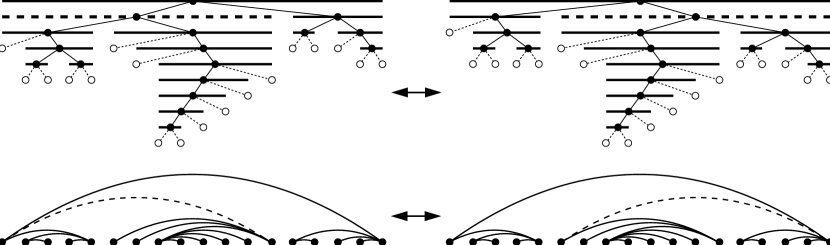
(((a((bc)(de))) (f(g(((((hi)j)k)l)m))))((no)(p(qr)))) $\ \longleftrightarrow\$ ((a((bc)(de)))((f(g(((((hi)j)k)l)m))) ((no)(p(qr)))))

Figure 5: The bijection between binary trees (up), non-crossing alternating trees (middle) and bracketings (bottom). The flipping operation in each case is shown, and the elements affected by the flip are highlighted.

Figure 5 gives an example of these correspondences, including the correspondence of the respective flipping operations: If we remove any edge $e\neq 1n$ from a non-crossing alternating tree $T$, there is precisely one other non-crossing alternating tree $T^{\prime}$ which shares the edges $T-\{e\}$ with $T$. This exchange operation corresponds under the above bijection to a tree rotation of the binary tree, and to a single application of the associative law (remove a pair of interior parentheses and insert another one in the only possible way) in a bracketing.

Observe that still we don’t know that all the non-crossing and alternating trees appear as vertices of $X_{g}$. But this is easy to prove: since $X_{g}$ is simple of dimension $d-2$, its graph is regular of degree $d-2$. And it is a subgraph of the graph of rotations between binary trees, which is also $(d-2)$-regular and connected. Hence, the two graphs coincide.

If we now look at faces of $\bar{X}_{g}$, rather than vertices, the tight edges for each of them form a non-crossing alternating forest. Such a forest $G$ is an expansive mechanism if and only if the edge $1n$ is not in $G$: If that edge is present, $p_{1}$ and $p_{n}$ are fixed and any other $p_{i}$ must approach one of the two. If the edge $1n$ is not present, then let $i$ be the maximum index for which $1i$ is present. Then the motion $v_{1}=\cdots=v_{i}=0<v_{i+1}=\cdots=v_{n}$ is an expansive flex of $G$.

Hence, $\bar{X}_{g}$ has a unique maximal bounded face, the facet given by the equation $v_{n}-v_{1}=g_{1n}$ and corresponding to the edge $1n$ alone. This facet is then an $(n-2)$-dimensional simple polytope that we denote $X_{g}$. The $n-2$ neighbors of each vertex $v$ correspond to the $n-2$ possible exchanges of edges different from $1n$ in the tree $E(v)$.

Theorem 5.10.

$X_{g}$ is a simple $(n-2)$-dimensional polytope whose face poset is that of the associahedron. Vertices are in one-to-one correspondence with the non-crossing alternating trees on $n$ vertices. Two vertices are adjacent if and only if the two non-crossing alternating trees differ in a single edge.

$\bar{X}_{g}$ is an unbounded polyhedron with the same vertex set as $X_{g}$. The extreme rays correspond to the non-crossing alternating trees with the edge $1n$ removed.

Proof.

Only the statement regarding the face poset remains to be proved. This can be proved in two ways: On the one hand, we already know that the graphs of $X_{g}$ and of the $(d-2)$-associahedron coincide (the latter being the graph of rotations between binary trees). And simple polytopes with the same graph have also the same face poset. (This is a result of Blind and Mani; see [28, Section 3.4]). As a second proof, the correspondence between non-crossing alternating trees and bracketings trivially extends to a correspondence between non-crossing alternating forests containing $1n$ and “partial bracketings” in a string of $n$ letters which include the parentheses enclosing the whole string. The poset of such things is the face poset of the associahedron (see [24], Proposition 6.2.1 and Exercise 6.33). In particular, the face-poset of $X_{g}$ is a subposet of the face-poset of the associahedron, and two polytopes of the same dimension cannot have their face posets properly contained in one another. This is true in general by topological reasons, but specially obvious in our case since we know our polytopes to be simple and their vertices to correspond one to one. Each vertex is incident to exactly $\binom{d-2}{i}$ faces of dimension $i$ in both polytopes, and two subsets of cardinality $\binom{d-2}{i}$ cannot be properly contained in one another. ∎

A result which is related to Theorem 5.10 was proved by Gelfand, Graev, and Postnikov [10, Theorem 6.3], in a setting dual to ours: there a triangulation of a certain polytope was constructed. The non-crossing alternating trees correspond to the simplices of the triangulation. It is shown explicitly that the simplices form a partition of the polytope. Certain numbers $g_{ij}$ are then associated with the vertices of the polytope to show that the triangulation is a projection of the boundary of a higher-dimensional polytope. Incidentally, the numbers that were suggested for this purpose are $(i-j)^{2}$, which coincides with the simple proposal given above after (14), but the calculations are not given in the paper [10].

One easily sees that the conditions $(\ref{eq:f4}$–$\ref{eq:f3})$ on $g$ are also necessary for the theorem to hold: If any of these conditions would hold as an equality or as an inequality in the opposite direction, the argument of Lemma 5.6 would work in the opposite direction, and certain non-crossing alternating trees would be excluded. Thus, $(\ref{eq:f4}$–$\ref{eq:f3})$ are a complete characterization of the “valid” parameter values $g_{ij}$.

Further Remarks.

The result we presented in this section is surprising in two ways: first, that it produces such a well studied object as the associahedron; second, that it requires additional types of linear constraints that are not needed in dimension $2$. Indeed, inequalities (13) in the 1-dimensional case are the exact analog of inequalities (8) in the 2-dimensional case, as we will see in Section 6. But the constraints (12) have no analog. This second aspect makes the task of producing $3$d generalization of the constructions of this paper more challenging, as there does not seem to be a straightforward pattern for producing the linear constraints whose instantiations in 1d and 2d give the polytopes of expansive motions.

The conditions (12–13) leave a lot of freedom for the choice of the variables $g_{ij}$. We have an ${\binom{n}{2}}$-dimensional parameter space. This is in contrast to the classical representation, which has $2n$ parameters (the coordinates of $n$ points in the plane). If we select the parameters to be integral, we obtain an associahedron which is an integral polytope (this is also true for the classical associahedron for a polygon with integer vertices.) But observe that, in fact, the associahedra obtained here are in a sense much more special than the classical associahedra obtained as secondary polytopes. They have $n-2$ pairs of parallel facets, given by the equations $v_{i}=v_{1}+g_{1i}$ and $v_{i}=v_{n}-g_{in}$ (i.e., corresponding to the pairs of edges $1i$ and $in$). See the right picture of Figure 4, where $n=5$. This is no surprise, since we have constructed our polytope by perturbing (a region of) a Coxeter arrangement, whose hyperplanes are in extremely non-general position.

One can check that classical associahedra have no parallel facets. Hence, are associahedra are not affinely equivalent to the classical ones. Recently, Chapoton, Fomin and Zelevinsky [5] have shown another construction of the associahedron having as facet normals the root system of type $A_{n}$ (more generally, they show a similar construction for all root systems). Still, our associahedra are not affinely equivalent to theirs: Comparing the right part of our Figure 4 with their Figure 2 we see that both are 3-dimensional associahedra with three pairs of parallel facets but in their realization the three remaining facets share a vertex while in ours they do not. It is however conceivable that they are related by projective transformations.

Figure 6: (a) The non-crossing alternating trees appear as a face of a ppt-polytope. (b) Another associahedron in the same ppt-polytope.

The non-crossing alternating trees also appear directly as a face of the ppt-polytope. Consider the configuration of points shown in Figure 6, consisting of a convex chain $\{p_{1},\ldots,p_{n}\}$ and an additional point $p_{0}$. The pseudotriangulations containing all the edges from $p_{0}$ to the other points (Figure 6a), correspond to the non-crossing alternating trees on $p_{1},\ldots,p_{n}$, forming an associahedron of dimension $n-2$. Another associahedron (of dimension $n-3$) appears as a different face of this ppt-polytope: the face corresponding to the edges of the convex chain (Figure 6b). These two faces are disjoint.

Relations to optimization and the Monge matrices.

Constraints of the form (11) are commonly found in project planning and critical path analysis. The variables $v_{i}$ represent unknown start times of tasks, and the constraints (11) specify waiting conditions between different tasks. For example, the minimization of $v_{n}-v_{1}$ is a longest path problem in an acyclic network. The different vertices of $X_{g}$ correspond to the different optimal solutions when we apply various linear objective functions.

Matrices $G=(g_{ij})$ with the property (12) are said to have the Monge property, if we set $g_{ii}=0$ and $g_{ij}=\infty$ for $i>j$. The Monge property has received a great deal of attention in optimization because it arises often in applications and it characterizes special classes of optimization problems that can be solved efficiently, see [4] for a survey.

The dual linear program of the linear programming problem (11) (with a suitable objective function) is a minimum-cost flow problem on an acyclic network with edges $ij$ for $1\leq i<j\leq n$, and cost coefficients $-g_{ij}$. Network flow is actually one of the oldest areas in optimization in which the Monge property has been applied, and where it has been shown that optimal solutions can be obtained by a greedy algorithm in certain cases. The non-crossing alternating trees are just the different possible subgraphs of those edges which carry flow in an optimal solution.

6 Towards a General Framework, in Arbitrary Dimension

To make more explicit the analogy between our 1d and 2d constructions we’ll rewrite the $1$d construction back in terms of inequalities (6) instead of (11). As we mentioned at the beginning of Section 5.3, the way to do this is to substitute $g_{i,j}=f_{i,j}/(p_{j}-p_{i})$ everywhere. In particular, the constraints (13) become

$$\frac{f_{ik}}{p_{i}-p_{k}}+\frac{f_{kl}}{p_{k}-p_{l}}+\frac{f_{il}}{p_{l}-p_{i}}>0.$$

But $w_{ik}=\frac{1}{p_{i}-p_{k}}$, $w_{kl}=\frac{1}{p_{k}-p_{l}}$ and $w_{il}=\frac{1}{p_{l}-p_{i}}$ define a self-stress on any 1-dimensional point set $\{p_{i},p_{k},p_{l}\}$. Hence, inequalities (13) are the exact analog of inequalities (8) of the 2d case. The difference is that in 2d these inequalities are necessary and sufficient for a choice of parameters to be “valid”, while in 1d we need the additional constraints (12), which do not follow from (13) as the following example shows:

$$g_{12}=g_{23}=g_{34}=1,\qquad g_{13}=g_{24}=2.2,\qquad g_{14}=3.3.$$

Let’s see what would be a generalization of the 1d and 2d cases to arbitrary dimension. For any finite point set $P=\{p_{1},\dots,p_{n}\}$ spanning $\mathbb{R}^{d}$ (in general position or not) there is a well-defined cone of expansive motions $\bar{X}_{0}$ of dimension $nd-\binom{d+1}{2}$, which is the positive region in the arrangement of hyperplanes defined by the constraints (4). Every choice of perturbation parameters $(f_{ij})_{i,j\in\{1,\dots,n\}}$, via inequalities (6), produces a polyhedron of constrained expansions $\bar{X}_{f}$, whose faces are in correspondence with some graphs embedded on $P$. If the $f_{ij}$’s are sufficiently generic, this polyhedron is simple and:

• The face poset of $\bar{X}_{f}$ is isomorphic to a subposet of the graphs embedded on $P$, ordered by reverse inclusion.

• The maximal graphs in this subposet are some of the infinitesimally minimally rigid frameworks on $P$.

• Adjacent vertices on the polyhedron correspond to graphs differing only by one edge.

The main question is whether there is a clever choice of the $f_{ij}$’s or a sensible choice of a special family of minimally rigid frameworks to be the vertices of the polyhedron which admits a nice and simple geometric characterization, as non-crossing alternating trees in 1d or pointed pseudo-triangulations in 2d do. In particular, what should be the analog of pointed pseudo-triangulations on a point set in general position in 3d? One difficulty is that the combinatorics of minimally rigid graphs in dimension three is not fully understood. Perhaps a good case to start with would be points in convex and general position in dimension $3$, for which the convex hull edges provide a very canonical minimally rigid framework to start with.

Another observation is that both in the 1d and 2d cases that we have treated here, the resulting polytope $\bar{X}_{f}$ has a unique maximal bounded face. This is related to the graph of flips between the special minimally rigid frameworks considered being connected and regular, which is an extra desirable property.

It would even be interesting to have a good generalization of the 2d case to point sets which are not in general position. If we use the 2d definition of $f$ from equations (9) with many points on a common line, there are solutions in which all the inequalities are tight. In this way we get essentially the one-dimensional expansion cone of Proposition 2.7, when we project all vectors $v_{i}$ on the direction of that line. (This is the same situation as when all relations (13) are satisfied as equations.) One way to get rid of this degeneracy is to “perturb the perturbations” by adding an infinitesimal component of the one-dimensional expansion parameters of Section 5.3: instead of $f$ we use $f^{(2)}_{ij}+\varepsilon f^{(1)}_{ij}$, where $f^{(2)}$ is valid for two-dimensional point sets, $f^{(1)}_{ij}$ satisfy the restrictions required for the 1d perturbation parameters, and $\varepsilon>0$ is sufficiently small. The situation would be like in Figure 6a when the points on the convex chain converge to being collinear. We have not further investigated this idea.

Another consideration which may help to treat degenerate point sets and arbitrary-dimensional ones is that the ideas in Section 5.1 generalize with not much difficulty under very weak general position assumptions. Let us first try to generalize Lemma 5.1. We need to decide what is the right analog of the statement in part (b). We propose the following. Remember that a circuit of a point set $P=\{p_{1},\dots,p_{n}\}\subset\mathbb{R}^{d}$ is a minimal affinely dependent subset. If $P$ is in general position, its set of circuits ${\cal C}(P)$ is $\binom{P}{d+2}$. In general, any set of $d+2$ points spanning $d$ dimensions contains a unique circuit, but this circuit can have less than $d+2$ elements. In any case, the complete graph on a circuit $C$ has (up to a constant factor) a unique self stress $(w_{ij})_{i,j\in C}$ with no vanishing $w_{ij}$, which is the one given by Lemma 2.5.

Let us consider the following linear maps:

$$M\colon\qquad\mathbb{R}^{dn}\quad \longrightarrow \quad\mathbb{R}^{\binom{n}{2}}$$

$$(v_{1},\dots,v_{n}) \longmapsto \langle v_{i}-v_{j},p_{i}-p_{j}\rangle,$$

$$\Delta\colon\qquad\mathbb{R}^{\binom{n}{2}}\quad \longrightarrow \qquad\mathbb{R}^{{\cal C}(P)}$$

$$\{f_{ij}\}_{ij\in{\binom{n}{2}}} \longmapsto \Big{\{}\sum_{ij\in C}w_{ij}f_{ij}\Big{\}}_{C\in{\cal C}(P)}.$$

$M$ is just the rigidity map of the complete graph on $P$. The equivalence of (b) and (c) in Lemma 5.1 can be rephrased as

$$\ker\Delta=\operatorname{Im}M,\hbox{ for every planar point set in general position.}$$

But in fact the same is true in arbitrary dimension and under much weaker assumptions than general position:

Proposition 6.1.

For any point set $P\subset\mathbb{R}^{d}$, $\operatorname{Im}M\subseteq\ker\Delta$. If $P$ has $d$ affinely independent points whose spanned hyperplane contains no other point of $P$, then the reversed inclusion also holds.

Proof.

That $\operatorname{Im}M\subset\ker\Delta$ (i.e., $\Delta\circ M=0$) is one direction of Lemma 2.4. To prove $\ker\Delta\subset\operatorname{Im}M$, let $f\in\mathbb{R}^{\binom{n}{2}}$ be such that $\sum_{ij\in C}w_{ij}f_{ij}=0$ for every circuit $C$. We want to find a motion $a=(a_{1},\dots,a_{n})$ for which $M(a)=f$. Without loss of generality assume that $p_{1},\dots,p_{d}$ are the claimed affinely independent points. Let us fix a motion $(a_{1},\dots,a_{d})$ for the first $d$ points satisfying the $\binom{d}{2}$ equations of the system $Ma=f$ concerning these points. This motion exists and is unique up to an arbitrary translational and rotational component, because the complete graph on any affinely independent point set is minimally infinitesimally rigid.

By assumption, $\{p_{1},\dots,p_{d},p_{i}\}$ is an affine basis for every $i>d$, and hence the complete graph on it is again minimally infinitesimally rigid. Thus, there is a motion $(a^{\prime}_{1},\dots,a^{\prime}_{d},a_{i})$ satisfying the $\binom{d+1}{2}$ corresponding equations of the system $Ma=f$. Adding translations and rotations we can assume $a^{\prime}_{j}=a_{j}$, $j=1,\dots,d$. So we have constructed a motion $(a_{1},\dots,a_{n})$ which restricts to the one chosen for the $d$ first points and which satisfies all the equations for pairs of points that include one of the first $d$.

It remains to show that the equations are also satisfied for the edges $kl$ with $k,l>d$. We follow the same idea as in the proof of Lemma 5.1. Our assumption on the point set implies that the unique circuit $C$ contained in $\{p_{1},\dots,p_{d},p_{k},p_{l}\}$ uses both $p_{k}$ and $p_{l}$. To simplify notation, assume that this circuit is $\{p_{1},\dots,p_{i},p_{k},p_{l}\}$. By Lemma 2.4, there is a feasible motion $(a^{\prime}_{1},\dots,a^{\prime}_{i},a^{\prime}_{k},a^{\prime}_{l})$. By translations and rotations we assume $a_{j}=a^{\prime}_{j}$ for $j=1,\dots,i$. Observe now the value of $\langle v-u,p_{j_{1}}-p_{j_{2}}\rangle$, for any of the points in the circuit and for any vectors $v$ and $u$, depends only on the projection of $v$ and $u$ to the affine subspace spanned by $C$. Since the complete graphs on $\{p_{1},\dots,p_{i}\}$, on $\{p_{1},\dots,p_{i},p_{k}\}$ and on $\{p_{1},\dots,p_{i},p_{l}\}$ are minimally infinitesimally rigid when motions are restricted to that subspace, we conclude that the projections of $a_{k}$ and $a_{l}$ to that affine subspace coincide with the projections of $a^{\prime}_{k}$ and $a^{\prime}_{l}$. In particular, $\langle a_{l}-a_{k},p_{l}-p_{k}\rangle=\langle a_{l}^{\prime}-a_{k}^{\prime},p_{l}-p_{k}\rangle=f_{kl}.$ ∎

Hence, Lemma 5.1 and its corollary, Lemma 5.2, hold in this generalized setting, with one equation per circuit instead of one equation per 4-tuple. The weakened general position assumption for $d$ of the points holds for every planar point set, since, by Sylvester’s theorem, any finite set of points in the plane, not all on a single line, has a line passing through only two of the points.

In dimension 3, however, the same is not true, and actually there are point sets for which $\operatorname{Im}M\neq\ker\Delta$. Consider the case of six points, three of them in one line and three in another, with the two lines being skew (not parallel and not crossing). These two sets of three points are the only two circuits in the point set. In particular, $\ker\Delta$ has at most codimension 2 in $\mathbb{R}^{15}$, i.e., it has dimension at least 13. On the other hand, $\operatorname{Im}M$ has at most the dimension of the reduced space of motions, $18-6=12$.

7 Final Comments

We describe some open questions and ideas for further research. The main questions related to this work are how to extend the constructions from dimensions $1$ and $2$ to $3$ and higher, and how to treat subsets in special position in 2d. The expectation is that this would give a coherent definition for “pseudo-triangulations” in higher dimensions. Some ideas in this direction have been mentioned in Section 6.

Is our choice of $f_{ij}$’s in Section 3 essentially unique? The set of valid choices for a fixed point set is open in $\mathbb{R}^{\binom{n}{2}}$. But, what if we restrict our attention to choices for which, as in Theorem 3.9, each $f_{ij}$ depends only on the points $p_{i}$ and $p_{j}$, and not the rest of the configuration? Observe that if we want this, then Theorem 3.7 provides an infinite set of conditions on the infinite set of unknowns $\{f(p,q):p,q\in\mathbb{R}^{2}\}$. It follows from Lemma 5.1 that adding to a valid choice $(f_{ij})_{i,j\in\{1,\dots,n\}}$ any vector $(\delta_{ij})_{i,j\in\{1,\dots,n\}}$ in the image of the rigidity map we still get a valid choice. And, of course, we can also scale any valid choice by a positive constant. This gives a half-space of valid choices of dimension ${\binom{n}{2}}+1$. Is this all of it?

It would also be interesting to see if there is a deeper reason behind Lemma 3.10. We have actually been able to extend the identity $\sum w_{ij}f_{ij}=1$ to a more general class of planar graphs than just the complete graph on four vertices: to wheels (graphs of pyramids). A wheel is a cycle with an additional vertex attached to every vertex of the cycle. For a wheel embedded in the plane in general position, formulas that are quite similar to (3) in Lemma 2.6 define a self-stress $w_{ij}$ on its edges which make the identity $\sum w_{ij}f_{ij}=1$ true. (Since the wheel is infinitesimally rigid and has $2n-2$ edges, the self-stress is unique up to a scalar factor.) We take this as a hint that the identity of Lemma 3.10 might be an instance of a more general phenomenon which we don’t fully understand.

Figure 7: (a) The Delaunay triangulation of a point set in convex position. (b-c) The triangulations minimizing and maximizing the objective function $(p_{1},\dots,p_{n})$ over the ppt-polytope, respectively. The triangulations in (b) and (c) are invariant under affine transformations, whereas (a) is not.

Another issue, with which we raised the introduction, is that having a representation of combinatorial structures as vertices of a polytope opens the way for selecting a particular structure, by optimizing some linear functional over the polytope. For example, the minimization of the objective function with coefficient vector $(|p_{1}|^{2},\dots,|p_{n}|^{2})$ over the secondary polytope gives the Delaunay triangulation. The opposite choice gives the furthest-site Delaunay triangulation. The most natural choice of objective function for the polytope of pointed pseudo-triangulations is $(p_{1},\dots,p_{n})$ or its opposite, i.e., minimize or maximize $\sum_{i}\langle p_{i},v_{i}\rangle$ over all constrained expansions which are tight on convex hull edges. Even if, for points in convex position, our ppt-polytope is affinely isomorphic to the secondary polytope, this functional on the ppt-polytope does not, in general, give the Delaunay triangulation of those points, see Figure 7. In fact, the result on the ppt-polytope is invariant under affine transformations of the point set, while the Delaunay triangulation is not. The properties of the pointed pseudo-triangulations that are defined in this way await further studies.

Added in proof.

The second author, together with David Orden, has extended the main construction of this paper to a simple polyhedron of dimension $3n-3$ with a unique maximal bounded face whose vertices are all the pseudo-triangulations of the point set. Bounded edges correspond to either classical edge-flips or to the creation or destruction of pointedness at a vertex by the deletion or inclusion of a single edge. The face poset of this polyhedron is (essentially) the poset of all non-crossing graphs on the point set.

About the Authors

Günter Rote is at the Institut für Informatik, Freie Universität Berlin, Takustraße 9, D-14195 Berlin, Germany, rote@inf.fu-berlin.de. Francisco Santos is at the Departamento de Matemáticas, Estadística y Computación, Universidad de Cantabria, E-39005 Santander, Spain, santos@matesco.unican.es. Ileana Streinu is at the Department of Computer Science, Smith College, Northampton, MA 01063, USA, streinu@cs.smith.edu.

References

- [1] Pankaj Agarwal, Julien Basch, Leonidas Guibas, John Hershberger, and Li Zhang, Deformable free space tilings for kinetic collision detection. in Bruce Randall Donald, Kevin Lynch and Daniela Rus (eds.), Algorithmic and Computational Robotics: New Directions, th Int. Workshop on Alg. Found. Robotics (WAFR), A K Peters, 2000, pp. 83–96.
- [2] David Avis and Komei Fukuda, Reverse search for enumeration. Discrete Appl. Math. 65 (1996), 21–46.
- [3] Hervé Brönnimann, Lutz Kettner, Michel Pocchiola, and Jack Snoeyink. Counting and enumerating pseudo-triangulations with the greedy flip algorithm. Manuscript, submitted for publication, 2001.
- [4] Rainer E. Burkard, Bettina Klinz, and Rüdiger Rudolf, Perspectives of Monge properties in optimization. Discrete Appl. Math. 70 (1996), 95–161.
- [5] Frederic Chapoton, Sergey Fomin, and Andrei Zelevinsky, Polytopal realizations of generalized associahedra, preprint math.CO/0202004, 25 pages, February 2002.
- [6] Robert Connelly, Erik D. Demaine, and Günter Rote, Straightening polygonal arcs and convexifying polygonal cycles. Discrete & Computational Geometry, to appear. Preliminary version in Proc. 41st Ann. Symp. on Found. of Computer Science (FOCS 2000), Redondo Beach, California; IEEE Computer Society Press, Washington, D.C., 2000, pp. 432–442; an extended version is available as technical report B 02-02, Freie Universität Berlin, Institut für Informatik, 2002.
- [7] Robert Connelly and Walter Whiteley, Second-order rigidity and prestress tensegrity frameworks. SIAM Journal on Discrete Mathematics 9 (1996), 453–491.
- [8] George B. Dantzig, Alan J. Hoffman, T. C. Hu, Triangulations (tilings) and certain block triangular matrices. Math. Programming 31 (1985), 1–14.
-
[9]
Komei Fukuda,
cdd code.
http://www.ifor.math.ethz.ch/staff/fukuda/fukuda.html - [10] Israel M. Gelfand, M. I. Graev, and Alexander Postnikov, Combinatorics of hypergeometric functions associated with positive roots. In: Arnold, V. I. et al. (ed.), The Arnold-Gelfand Mathematical Seminars: Geometry and Singularity Theory. Boston, Birkhäuser. pp. 205–221 (1997)
- [11] Israel M. Gel′fand, Andrei V. Zelevinskiǐ, and M. M. Kapranov, Discriminants of polynomials in several variables and triangulations of Newton polyhedra. Leningrad. Math. J. 2 (1991), 449–505, translation from Algebra Anal. 2 (1990), No. 3, 1–62.
- [12] Michael Goodrich and Roberto Tamassia, Dynamic ray shooting and shortest paths in planar subdivisions via balanced geodesic triangulations. J. Algorithms 23 (1997), 51–73.
- [13] Jack Graver, Brigitte Servatius, and Hermann Servatius, Combinatorial Rigidity. AMS Graduate Studies in Mathematics vol. 2, 1993.
- [14] David Kirkpatrick, Jack Snoeyink, and Bettina Speckmann, Kinetic collision detection for simple polygons. International Journal of Computational Geometry and Applications 12 (2002), 3–27. Extended abstract in Proc. 16th Ann. Symposium on Computational Geometry, pp. 322–330, 2000.
- [15] G. Laman, On graphs and rigidity of plane skeletal structures. J. Engineering Math. 4 (1970), 331–340.
- [16] Carl Lee, The associahedron and triangulations of the -gon. European J. Combinatorics 10 (1989), 551–560.
- [17] Jesús A. de Loera, Serkan Hoşten, Francisco Santos, and Bernd Sturmfels, The polytope of all triangulations of a point configuration. Documenta Mathematica, J. DMV 1 (1996), 103–119.
- [18] Michel Pocchiola and Gert Vegter, Topologically sweeping visibility complexes via pseudo-triangulations. Discr. & Comput. Geometry 16 (1996), 419–453.
- [19] Michel Pocchiola and Gert Vegter, The visibility complex. Int. J. Comput. Geom. Appl. 6 (1996), 279–308.
- [20] Michel Pocchiola and Gert Vegter, Pseudo-triangulations: Theory and applications. In Proc. 12th Ann. ACM Sympos. Comput. Geom., ACM Press, May 1996, pp. 291–300.
- [21] Alexander Postnikov, Intransitive trees. J. Combin. Theory, Ser. A 79 (1997), 360–366.
- [22] Alexander Postnikov and Richard P. Stanley, Deformations of Coxeter hyperplane arrangements. J. Combin. Theory, Ser. A 91 (2000), 544–597.
- [23] B. Speckmann and C. D. Tóth, Vertex -guards in simple polygons. In Abstracts of the 18th European Workshop on Computational Geometry (EuroCG), April 10–12, 2002, Warszawa, Poland, pp. 12–15. Full version submitted for publication.
- [24] Richard Stanley, Enumerative Combinatorics. Vol. 2, Cambridge University Press, 1999.
- [25] Ileana Streinu, A combinatorial approach to planar non-colliding robot arm motion planning, In Proc. 41st Ann. Symp. on Found. of Computer Science (FOCS 2000), Redondo Beach, California, November 2000, pp. 443–453.
- [26] Ileana Streinu, A combinatorial approach to planar non-colliding robot arm motion planning, preprint, 2002.
- [27] Walter Whiteley, Rigidity and Scene Analysis, in: Jacob E. Goodman and Joseph O’Rourke (eds.) Handbook of Discrete and Computational Geometry, CRC Press, 1997, pp. 893–916.
- [28] Günter Ziegler, Lectures on Polytopes (2nd ed.), Springer-Verlag, 1999.