Hyperbolic constant mean curvature one surfaces: Spinor representation and trinoids in hypergeometric functions

1 Introduction

 

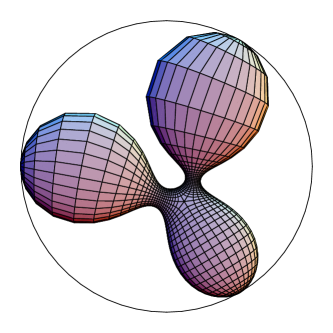
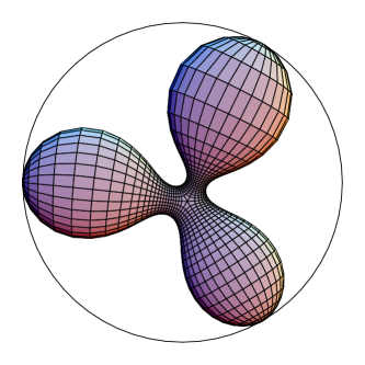
Fig. 1: Non-symmetric trinoids

For minimal surfaces in $\mathbb{R}^{3}$ there is a representation, due to Weierstrass, in terms of holomorphic data. The Gauss-Codazzi equations for minimal surfaces in $\mathbb{R}^{3}$ are equivalent to those for surfaces in hyperbolic space with constant mean curvature 1 (CMC-1 surfaces). This lead Bryant [Br] to derive a representation for CMC-1 surfaces in terms of holomorphic data.

The holomorphic data used in the Weierstrass representation for minimal surfaces consists alternatively of a function and a one-form, or of two spinors with the same spin structure [Bo, KS]. These functions, forms, and spinors are defined on the same Riemann surface as the conformal minimal immersion which they represent. Bryant’s representation for CMC-1 surfaces also involves two spinors with the same spin structure. Other researchers prefer an equivalent version involving a function and a one-form [UY93, CHR]. But the functions, forms, and spinors that comprise the holomorphic data for Bryant’s representation are not defined on the same Riemann surface as the conformal immersion they represent. As a result, a considerable amount of the great power of complex function theory is lost. In particular, Bryant’s representation does not yield explicit formulas for CMC-1 surfaces unless their topology is very simple.

In this paper, we present a different representation for CMC-1 surfaces in terms of holomorphic spinors which are defined on the same Riemann surface as the immersion. This global representation is only a slight modification of Bryant’s representation, but it is much more useful if one wants to derive explicit formulas for CMC-1 surfaces. We present a derivation of both representations based on the method of moving frames.

We use the global representation to derive explicit formulas for CMC-1 surfaces of genus $0$ with three regular ends which are asymptotic to catenoid cousins (CMC-1 trinoids). These surfaces were classified by Umehara and Yamada [UY96], but they do not present explicit formulas.

2 The spinor representation of surfaces in $\mathbb{H}^{3}$

Minkowski 4-space $\mathcal{L}^{4}$ with the canonical Lorentzian metric of signature $(-,+,+,+)$ can be represented as the space of $2\times 2$ hermitian matrices. We identify $(x_{0},x_{1},x_{2},x_{3})\in\mathcal{L}^{4}$ with the matrix

$$X=x_{o}I+\sum_{\alpha=1}^{3}x_{\alpha}\overline{\sigma}_{\alpha}=\begin{pmatrix}x_{0}+x_{3}&x_{1}+ix_{2}\\ x_{1}-ix_{2}&x_{0}-x_{3}\end{pmatrix}\in\operatorname{Herm}(2).$$

where $\overline{\sigma}_{\alpha}$ are complex conjugate Pauli matrices

$$\overline{\sigma}_{1}=\begin{pmatrix}0&1\\ 1&0\end{pmatrix}=\sigma_{1},\overline{\sigma}_{2}=\begin{pmatrix}0&i\\ -i&0\end{pmatrix}=-\sigma_{2},\overline{\sigma}_{3}=\begin{pmatrix}1&0\\ 0&-1\end{pmatrix}=\sigma_{3}.$$

In terms of the corresponding matrices the scalar product of vectors $X$ and $Y$ is

$$\langle X,\,Y\rangle\,=\,-\frac{1}{2}\;\operatorname{tr}(X\,\sigma_{2}\,Y^{T}\,\sigma_{2}).$$

Under this identification, hyperbolic 3-space

$$\mathbb{H}^{3}=\{(x_{0},x_{1},x_{2},x_{3})\in\mathcal{L}^{4};\sum_{i=1}^{3}x_{i}^{2}-x_{0}^{2}=-1,x_{0}>0\}$$

is represented as

$$\mathbb{H}^{3} =\{X\in\operatorname{Herm}(2);\langle X,X\rangle=-1=-\det(X),\operatorname{tr}(X)>0\}$$

$$=\{a\cdot a^{*};a\in\operatorname{\mathit{SL}}(2,\mathbb{C})\},$$

where $a^{*}=\overline{a}^{T}$.

Consider a smooth orientable surface in hyperbolic 3-space. The induced metric $\Omega$ generates the complex structure of a Riemann surface $\mathcal{R}$. The surface is given by an immersion $F=(F_{0},F_{1},F_{2},F_{3}):\,\mathcal{R}\,\to\mathbb{H}^{3},$ and the metric is conformal: $\Omega=e^{u}\,dzd\bar{z}$ where $z=x+iy$ is a local coordinate on $\mathcal{R}$. The conformality of the parameterization is equivalent to

$$\langle F_{z},\,F_{z}\rangle=\langle F_{\overline{z}},\,F_{\overline{z}}\rangle=0,\quad\langle F_{z},\,F_{\overline{z}}\rangle=\frac{1}{2}\,e^{u}.$$

Here $F_{z},F_{\overline{z}}$ are the partial derivatives with

$$\frac{\partial}{\partial z}=\frac{1}{2}(\frac{\partial}{\partial x}-i\,\frac{\partial}{\partial y}),\quad\frac{\partial}{\partial\overline{z}}=\frac{1}{2}(\frac{\partial}{\partial x}+i\,\frac{\partial}{\partial y}).$$

The vectors $F,F_{x},F_{y}$ and the unit normal $N$ define an orthogonal moving frame on the surface

$$\langle F,F\rangle=-1,\quad\langle N,N\rangle=1.$$

The first and the second fundamental forms are

$$\langle dF,\,dF\rangle =e^{u}\,dz\,d\overline{z},$$

$$-\langle dF,\,dN\rangle =Q\,dz^{2}+H\,e^{u}\,dz\,d\overline{z}+\overline{Q}\,d\overline{z}^{2},$$

where

$$Q=\langle F_{z\,z},\,N\rangle,\quad H\,e^{u}=2\,\langle F_{z\,\overline{z}},\,N\rangle.$$

Here, $Q\,dz^{2}$ is the Hopf differential and $H$ is the mean curvature of $F$.

Conformal immersions in ${\mathbb{H}}^{3}$ can be described locally, on a domain $D\subset{\mathbb{C}}$, by a smooth mapping $\varphi:\,D\,\to\operatorname{\mathit{SL}}(2,\mathbb{C})$ which transforms the basis $I,\overline{\sigma}_{1},\overline{\sigma}_{2},\overline{\sigma}_{3}$ into the moving frame $F,F_{x},\,F_{y},\,N$:

$$F =\varphi\,\varphi^{*},$$

$$F_{x} =e^{u/2}\,\varphi\,\overline{\sigma}_{1}\,\varphi^{*},$$

$$F_{y} =e^{u/2}\,\varphi\,\overline{\sigma}_{2}\,\varphi^{*},$$

$$N =\varphi\,\overline{\sigma}_{3}\,\varphi^{*}.$$

In the complex coordinate $z=x+iy$ we have

$$dF=e^{u/2}\,\varphi\,\begin{pmatrix}0&dz\\ d\overline{z}&0\end{pmatrix}\,\varphi^{*}.$$

The Gauss-Weingarten equations in terms of $\varphi$ are

$$\varphi_{z} =\varphi\,\widetilde{U}, \qquad\widetilde{U} =\begin{pmatrix}u_{z}/4&\frac{1}{2}\,(H+1)\,e^{u/2}\\ -Q\,e^{-u/2}&-u_{z}/4\end{pmatrix},$$ (2.1)

$$\varphi_{\overline{z}} =\varphi\,\widetilde{V}, \qquad\widetilde{V} =\begin{pmatrix}-u_{\overline{z}}/4&\overline{Q}\,e^{-u/2}\\ -\frac{1}{2}\,(H-1)\,e^{u/2}&u_{\overline{z}}/4\end{pmatrix}.$$ (2.2)

Their compatibility condition are the Gauss-Codazzi equations

$$u_{z\,\overline{z}}\,+\,\frac{1}{2}\,(H^{2}-1)\,e^{u}\,-\,2\,Q\,\overline{Q}\,e^{-u} =0,$$ (2.3)

$$\overline{Q}_{z}=\frac{1}{2}\,H_{\overline{z}}\,e^{u},$$

$$Q_{\overline{z}}=\frac{1}{2}\,H_{z}\,e^{u}.$$

Globally, not $\varphi$ but

$$\Phi\,\begin{pmatrix}\sqrt{dz}&0\\ 0&\sqrt{d\overline{z}}\end{pmatrix}$$ (2.4)

is well defined, where $\Phi=e^{u/4}\,\varphi$. This is a spinor on the Riemann surface $\mathcal{R}$; it is independent of the choice of a local coordinate $z$ on $\mathcal{R}$. Note that $\det\Phi=e^{u/2}$.

We arrive at the following

Theorem 1.

A conformal immersion $F:{\mathcal{R}}\to{\mathbb{H}}^{3}$ with Gauss map $N$ defines, uniquely up to sign, a spinor (2.4) on $\mathcal{R}$ such that locally

$$F =e^{-u/2}\Phi\,\Phi^{*},$$ (2.5)

$$dF =\Phi\,\begin{pmatrix}0&dz\\ d\overline{z}&0\end{pmatrix}\Phi^{*},$$

$$N =e^{-u/2}\Phi\,\overline{\sigma}_{3}\,\Phi^{*}.$$

Furthermore, $e^{u/2}=\det\Phi$ and

$$\Phi^{-1}\,\Phi_{z} =U, \qquad U =\begin{pmatrix}u_{z}/2&\frac{1}{2}\,(H+1)\,e^{u/2}\\ -Q\,e^{-u/2}&0\end{pmatrix},$$ (2.6)

$$\Phi^{-1}\,\Phi_{\overline{z}} =V, \qquad V =\begin{pmatrix}0&\overline{Q}\,e^{-u/2}\\ -\frac{1}{2}\,(H-1)\,e^{u/2}&u_{\overline{z}}/2\end{pmatrix}.$$

Conversely, given a spinor (2.4) on $\mathcal{R}$ with $\Phi$ satisfying (2.6), where $e^{u/2}=\det\Phi$, formulas (2.5) describe a conformally parametrized surface in $\mathbb{H}^{3}$ and its Gauss map $N$.

3 The Weierstrass representation for CMC-1 surfaces in $\mathbb{H}^{3}$

Let $F$ be a surface in $\mathbb{H}^{3}$ with constant mean curvature $H=1$ (CMC-1 surface). The corresponding $\Phi$ of theorem 1 satisfies

$$\Phi_{z} =\Phi\,U, \qquad U =\begin{pmatrix}u_{z}/2&e^{u/2}\\ -Q\,e^{-u/2}&0\end{pmatrix},$$ (3.1)

$$\Phi_{\overline{z}} =\Phi\,V, \qquad V =\begin{pmatrix}0&\overline{Q}\,e^{-u/2}\\ 0&u_{\overline{z}}/2\end{pmatrix},$$

Since, by the second equation, the $\overline{z}$-derivative of the first column of $\Phi$ vanishes,

$$\Phi=\begin{pmatrix}{\mathsf{P}}&*\\ {\mathsf{Q}}&*\end{pmatrix},$$ (3.2)

where ${\mathsf{P}}$ and ${\mathsf{Q}}$ are holomorphic spinors on $\mathcal{R}$; see (2.4). Furthermore, the first equation of (3.1), equation (3.2), and $\det\Phi=e^{u/2}$ imply that the Hopf differential is related to ${\mathsf{P}}$ and ${\mathsf{Q}}$ by

$$Q={\mathsf{P}}^{\prime}{\mathsf{Q}}-{\mathsf{Q}}^{\prime}{\mathsf{P}}.$$ (3.3)

The hyperbolic Gauss map (see [UY96]) is

$$G=-{\mathsf{P}}/{\mathsf{Q}}.$$ (3.4)

Setting $H=1$ in (2.3), one obtains the Gauss-Codazzi equations for CMC-1 surfaces:

$$u_{z\,\overline{z}}\,-\,2\,Q\,\overline{Q}\,e^{-u} =0,$$

$$Q_{\overline{z}}=0.$$

They are invariant with respect to the transformation

$$Q \to\lambda\,Q,$$ (3.5)

$$e^{u} \to|\lambda|^{2}\,e^{u},\qquad\lambda\in\mathbb{C}\setminus\{0\}.$$

Thus, every CMC-1 surface $F$ in $\mathbb{H}^{3}$ possesses a two-parameter family $F_{\lambda}$ of deformations (3.5) within the CMC-1 class.

Consider the corresponding $\Phi(z,\,\overline{z},\,\lambda)$ which is a solution of the system

$$\Phi_{z} =\Phi\,U(\lambda), \qquad U(\lambda) =\begin{pmatrix}u_{z}/2&|\lambda|e^{u/2}\\ -\frac{\lambda}{|\lambda|}Q\,e^{-u/2}&0\end{pmatrix},$$ (3.6)

$$\Phi_{\overline{z}} =\Phi\,V(\lambda), \qquad V(\lambda) =\begin{pmatrix}0&\frac{\overline{\lambda}}{|\lambda|}\overline{Q}\,e^{-u/2}\\ 0&u_{\overline{z}}/2\end{pmatrix}.$$ (3.7)

Now let $\lambda\rightarrow 0$ while $\frac{\lambda}{|\lambda|}=1$. The corresponding equations have solutions of the form

$$\Phi_{0}=\begin{pmatrix}{\mathsf{p}}&\overline{\mathsf{q}}\\ -{\mathsf{q}}&\overline{\mathsf{p}}\end{pmatrix}$$ (3.8)

where ${\mathsf{p}}$ and ${\mathsf{q}}$ are holomorphic spinors on the universal covering $\widetilde{\mathcal{R}}$ of $\mathcal{R}$, and

$$\begin{split}e^{u/2}&=|{\mathsf{p}}|^{2}+|{\mathsf{q}}|^{2},\\ Q&=-{\mathsf{p}}^{\prime}{\mathsf{q}}+{\mathsf{p}}{\mathsf{q}}^{\prime}.\end{split}$$ (3.9)

Remark.

Note that ${\mathsf{P}}$ and ${\mathsf{Q}}$ are well defined holomorphic spinors on the Riemann surface $\mathcal{R}$, but the spinors ${\mathsf{p}}$ and ${\mathsf{q}}$ are only well defined on the universal cover $\widetilde{\mathcal{R}}$ of $\mathcal{R}$.

Let $\Phi_{1}=\Phi|_{\lambda=1}$ and denote by $\Psi$ the quotient

$$\Phi_{1}\,=\,\Psi\,\Phi_{0}\,.$$ (3.10)

Theorem 2.

The mapping $\Psi:\widetilde{\mathcal{R}}\to\operatorname{\mathit{SL}}(2,\mathbb{C})$ defined by (3.10) is holomorphic and satisfies

$$\Psi_{z} =\Psi\begin{pmatrix}{\mathsf{p}}{\mathsf{q}}&{\mathsf{p}}^{2}\\ -{\mathsf{q}}^{2}&-{\mathsf{p}}{\mathsf{q}}\end{pmatrix},$$ (3.11)

$$\Psi_{z} =\begin{pmatrix}{\mathsf{P}}{\mathsf{Q}}&{\mathsf{P}}^{2}\\ -{\mathsf{Q}}^{2}&-{\mathsf{P}}{\mathsf{Q}}\end{pmatrix}\Psi,$$ (3.12)

where ${\mathsf{p}}$, ${\mathsf{q}}$ are the holomorphic spinors on $\widetilde{\mathcal{R}}$ defined by (3.8), and ${\mathsf{P}}$, ${\mathsf{Q}}$ are the holomorphic spinors on $\mathcal{R}$ defined by (3.2).

The immersion $F:\mathcal{R}\to\mathbb{H}^{3}$ is recovered by

$$F=\Psi\Psi^{*}.$$ (3.13)

Proof.

Since

$$\Psi_{\overline{z}}=(\Phi_{1}\,{\Phi_{0}}^{-1})_{\overline{z}}=\Phi_{1}({\Phi_{1}}^{-1}\Phi_{1\,\overline{z}}-{\Phi_{0}}^{-1}\Phi_{0\,\overline{z}}){\Phi_{0}}^{-1},$$

equations (3.6) imply $\Psi_{\overline{z}}=0$. Hence $\Psi$ is holomorphic.

Similarly one finds that,

$$\Psi_{z}=e^{u/2}\Phi_{1}\begin{pmatrix}0&1\\ 0&0\end{pmatrix}\Phi_{0}^{-1},$$

and hence,

$$\Psi^{-1}\,\Psi_{z}\,=\,e^{u/2}\,\Phi_{0}\,\begin{pmatrix}0&1\\ 0&0\end{pmatrix}\,\Phi_{0}^{-1}$$

and

$$\Psi_{z}\,\Psi^{-1}\,=\,e^{u/2}\,\Phi_{1}\,\begin{pmatrix}0&1\\ 0&0\end{pmatrix}\,\Phi_{1}^{-1}.$$

Now, (3.8) and (3.2) imply (3.11), (3.12). Finally, equation (2.5) and $\Phi_{0}{\Phi_{0}}^{*}=e^{u/2}I$ imply the immersion formula (3.13). ∎

By equation (3.11) and the immersion formula (3.13), the spinors ${\mathsf{p}}$ and ${\mathsf{q}}$ determine the surface $F$ up to a hyperbolic isometry. The metric and Hopf differential are related to ${\mathsf{p}}$ and ${\mathsf{q}}$ by (3.9). This representation of CMC-1 surfaces, which is due to Bryant [Br], is therefore an intrinsic and metric description. It is also essentially local, since the spinors ${\mathsf{p}}$ and ${\mathsf{q}}$ are not well defined on the Riemann surface $\mathcal{R}$, but only on its universal cover. This is a serious disadvantage if one wants to construct CMC-1 surfaces with non-trivial topology. In particular, this prohibits in all but the simplest cases the integration of equation (3.11) in closed form.

Formula (3.12), on the other hand, is a global representation of a CMC-1 surface by holomorphic spinors ${\mathsf{P}}$ and ${\mathsf{Q}}$ on $\mathcal{R}$. Unfortunately, these spinors do in general not determine the surface up to isometry. While the Hopf differential and the hyperbolic Gauss map are determined by (3.3) and (3.4), the metric depends non-trivially on the particular solution of (3.12). But there is also the global condition that the immersion $F$ obtained from (3.13) is well defined on $\mathcal{R}$. This, together with ${\mathsf{P}}$ and ${\mathsf{Q}}$, may determine the surface uniquely if $\mathcal{R}$ is not simply connected. The condition that $F$ is well defined on $\mathcal{R}$ implies the following corollary.

Corollary 1.

Let $F:\mathcal{R}\to\mathbb{H}^{3}$ be a CMC-1 surface in $\mathbb{H}^{3}$ and $\Phi$ its spinor frame (3.2), defining holomorphic spinors ${\mathsf{P}}$ and ${\mathsf{Q}}$ on $\mathcal{R}$. Then equation (3.12) has a solution $\Psi:\widetilde{\mathcal{R}}\to\operatorname{\mathit{SL}}(2,\mathbb{C})$ with unitary monodromy.

Conversely, one obtains the following representation theorem.

Theorem 3.

Let ${\mathsf{P}}$ and ${\mathsf{Q}}$ be two holomorphic spinors with the same spin structure on a Riemann surface $\mathcal{R}$ and suppose $\Psi:\widetilde{\mathcal{R}}\to\operatorname{\mathit{SL}}(2,\mathbb{C})$ a solution of equation (3.12) with unitary monodromy. Then equation (3.13) defines a CMC-1 immersion $F:{\mathcal{R}}\to\mathbb{H}^{3}$.

Rossman, Umehara, Yamada, and others describe CMC-1 surfaces in terms of the ‘secondary Gauss map’ $g=-{\mathsf{p}}/{\mathsf{q}}$ and the one-form $\omega=-{\mathsf{q}}^{2}\,dz$. Thus, instead of equation (3.11), they write

$$d\Psi=\Psi\begin{pmatrix}g&-g^{2}\\ 1&-g\end{pmatrix}\omega.$$

The secondary Gauss map $g$ and one-form $\omega$ are not defined on the same Riemann surface $\mathcal{R}$ on which the conformal immersion $F$ is defined. The hyperbolic Gauss map $G=-{\mathsf{P}}/{\mathsf{Q}}$ and the holomorphic one-form $\Omega=-{\mathsf{Q}}^{2}\,dz$, one the other hand, are defined on the Riemann surface $\mathcal{R}$. In terms of these, equation (3.12) reads

$$d\Psi=\begin{pmatrix}G&-G^{2}\\ 1&-G\end{pmatrix}\Psi\Omega.$$

Even though Rossman, Umehara and Yamada are aware of this equation [RUY], they do not consider $G$ and $\Omega$ as the Weierstrass data for the CMC-1 immersion $F$ but for a dual immersion.

4 Catenoid cousin, catenoidal ends and n-noids

 

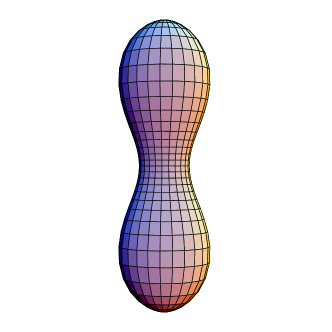
(a) $\lambda<\tfrac{1}{2}$

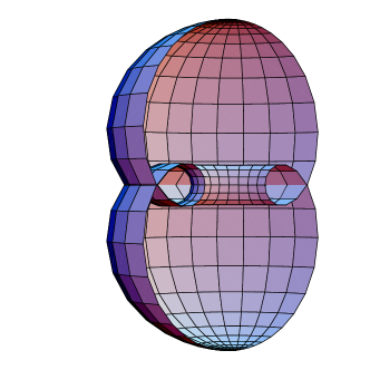
(b) $\lambda>\tfrac{1}{2}$

Fig. 2: CMC-1 twonoids in the Poincaré model of $\mathbb{H}^{3}$.

Let us start our investigation of special CMC-1 surfaces in $\mathbb{H}^{3}$ with a simple example of the catenoid cousins which we also call twonoids. Since the Gauss equations of CMC-1 surfaces in $\mathbb{H}^{3}$ and of minimal surfaces in $\mathbb{R}^{3}$ coincide these surfaces are locally isometric. The catenoid cousins are surfaces isometric to the catenoids. They were investigated by Bryant [Br].

These surfaces are of genus zero with two regular ends. In our global spinorial description, twonoids are immersions

$$F=\Psi\Psi^{*}:\mathbb{C}\setminus\{0\}\to\mathbb{H}^{3},$$

where $\Psi$ satisfies the differential equation (3.12) with the Weierstrass data

$${\mathsf{P}}=\frac{p_{0}}{z}+p_{\infty},\qquad{\mathsf{Q}}=\frac{q_{0}}{z}+q_{\infty}.$$

(By applying a suitable hyperbolic isometry and a coordinate transformation $z\to az$ to $F$ one can reduce this to the simpler case $p_{0}=q_{\infty}=0$, $p_{\infty}=q_{0}$.) This equation can be solved explicitly in elementary functions. A particular solution with determinant 1 is

$$\Psi_{0}=cB\begin{pmatrix}z^{1/2}&0\\ 0&z^{-1/2}\end{pmatrix}C\begin{pmatrix}z^{\lambda}&0\\ 0&z^{-\lambda}\end{pmatrix},$$

where

$$B =\begin{pmatrix}\left(\frac{p_{0}}{z}+p_{\infty}\right)&\frac{p_{0}}{p_{0}q_{\infty}-p_{\infty}q_{0}}\\ -\left(\frac{q_{0}}{z}+q_{\infty}\right)&-\frac{q_{0}}{p_{0}q_{\infty}-p_{\infty}q_{0}}\end{pmatrix},$$

$$C =\begin{pmatrix}\frac{2\lambda-1}{2(p_{0}q_{\infty}-p_{\infty}q_{0})}&-\frac{2\lambda+1}{2(p_{0}q_{\infty}-p_{\infty}q_{0})}\\ 1&1\end{pmatrix},$$

$$\lambda=\frac{1}{2}\sqrt{1+4(p_{0}q_{\infty}-p_{\infty}q_{0})},\quad c=\sqrt{\frac{p_{0}q_{\infty}-p_{\infty}q_{0}}{2\lambda}}.$$

The general solution with determinant 1 is $\Psi=\Psi_{0}A$, with $A\in\operatorname{\mathit{SL}}(2,\mathbb{C})$. Since multiplying $A$ on the right with a unitary matrix does not change the immersion $F$, we may assume $A$ to be hermitian. When continued along a path going around the puncture $z=0$ in the counterclockwise direction, $\Psi$ is transformed into $\Psi\mathcal{M}_{0}$, where the monodromy matrix is

$$\mathcal{M}_{0}=-A^{-1}\begin{pmatrix}e^{2\pi i\lambda}&0\\ 0&e^{-2\pi i\lambda}\end{pmatrix}A.$$

For $\mathcal{M}_{0}$ to be unitary, $\lambda$ must be real. If $\lambda$ is not half-integer, then $A$ must be diagonal. In fact, it suffices to consider $A=I$, since different $A$ yield the same surface up to a hyperbolic isometry and a coordinate change $z\to az$. If $\lambda$ is half-integer, then $A$ is arbitrary. In this case, one obtains also surfaces which are not surfaces of revolution, and which are not locally isometric to a catenoid.

For the surfaces of revolution, the profile curve is embedded if $\lambda<\frac{1}{2}$, and it has a single self-intersection if $\lambda>\frac{1}{2}$, see Fig. 2.

There are no compact CMC-1 surfaces in $\mathbb{H}^{3}$. Bryant has shown that the Riemann surface of a complete conformal immersion $F:\mathcal{R}\to\mathbb{H}^{3}$ of finite total curvature can be compactified: $\mathcal{R}=\hat{\mathcal{R}}\setminus\left\{a_{1},a_{2},\dotsc,a_{N}\right\}$, where $\hat{\mathcal{R}}$ is a compact Riemann surface [Br]. Moreover, Collin, Hauswirth, and Rosenberg have shown that a properly embedded annular end is of finite total curvature and regular [CHR]. The punctures $a_{1},a_{2},\dotsc,a_{N}$ correspond to the ends of the immersion. For their classification one uses the hyperbolic Gauss map $G=-{\mathsf{P}}/{\mathsf{Q}}$. The end corresponding to a point $a_{i}\in\hat{\mathcal{R}}$ is called regular if $G$ can be meromorphically extended to $a_{i}$, and irregular if it is an essential singularity of $G$. Motivated by the behavior of the Weierstrass data at the punctures of twonoids, it is natural to give the following analytic definition of the catenoidal ends.

Definition 1.

The end corresponding to a puncture $a_{i}$, is called catenoidal, if the spinors ${\mathsf{P}}$, ${\mathsf{Q}}$ have only simple poles at $a_{i}$.

I. e., it is required that, for a local coordinate $z$ centered in $a_{i}$, the Weierstrass data ${\mathsf{P}}$, ${\mathsf{Q}}$ satisfy

$${\mathsf{P}}=\frac{p_{0}}{z}+O(1)\quad\text{and}\quad{\mathsf{Q}}=\frac{q_{0}}{z}+O(1)\quad\text{for}\quad z\to 0.$$

Obviously, catenoidal ends are regular.

We call a compact CMC-1 surface of genus zero with $n$ catenoidal ends an $n$-noid. Normalizing one end to $z=\infty$, all $n$-noids can be conformally parametrized as

$$F:\mathbb{C}\setminus\{a_{1},a_{2},\dotsc,a_{n-1}\}\to\mathbb{H}^{3}$$

with the Weierstrass data

$${\mathsf{P}}=\sum_{i=1}^{N-1}\frac{p_{i}}{z-z_{i}}+p_{\infty},\quad{\mathsf{Q}}=\sum_{i=1}^{N-1}\frac{q_{i}}{z-z_{i}}+q_{\infty}.$$ (4.1)

At a catenoidal end, the system (3.12) is locally gauge equivalent to a Fuchsian system. Indeed, let $z=0$ be a puncture and suppose ${\mathsf{P}}$ and ${\mathsf{Q}}$ satisfy

$${\mathsf{P}}=\frac{a_{-1}}{z}+a_{0}+o(1),\quad{\mathsf{Q}}=\frac{b_{-1}}{z}+b_{0}+o(1)\quad\text{for}\quad z\to 0.$$ (4.2)

The following lemma is obtained by direct calculation.

Lemma 1.

If $\Psi$ satisfies equation (3.12) with ${\mathsf{P}}$, ${\mathsf{Q}}$ as in (4.2), then the gauge equivalent $\widetilde{\Psi}$ defined by

$$\Psi=\begin{pmatrix}a_{-1}&0\\ -b_{-1}&\frac{1}{a_{-1}}\end{pmatrix}\,\begin{pmatrix}\frac{1}{\sqrt{z}}&0\\ 0&\sqrt{z}\end{pmatrix}\widetilde{\Psi}$$

satisfies an equation $\widetilde{\Psi}_{z}=\widetilde{A}\widetilde{\Psi}$, with

$$\widetilde{A}=\frac{1}{z}\begin{pmatrix}\frac{1}{2}+r&1\\ -r^{2}&-\frac{1}{2}-r\end{pmatrix}+O(1)\quad\text{for}\quad z\to\infty,$$

where $r=a_{-1}b_{0}-a_{0}b_{-1}$.

Corollary 2.

Under the conditions of the lemma, the local monodromy of (3.12) around $z=0$ is

$$M=\begin{pmatrix}e^{2\pi i\alpha}&0\\ 0&e^{-2\pi i\alpha}\end{pmatrix}\quad\text{with}\quad\alpha=\frac{1}{2}+\sqrt{\frac{1}{4}+r}.$$

5 Trinoids. Reduction to a Fuchsian system

The rest of the paper is devoted to explicit description of the trinoids, which are CMC-1 immersions of genus zero with three catenoidal ends. Without loss of generality the punctures can be normalized to $0,1,\infty$. By equation (4.1), the trinoids are thus conformal immersions $F:\mathbb{C}\setminus\{0,1\}\to\mathbb{H}^{3}$ with Weierstrass data

$${\mathsf{P}}=\frac{p_{0}}{z}+\frac{p_{1}}{z-1}+p_{\infty},\quad{\mathsf{Q}}=\frac{q_{0}}{z}+\frac{q_{1}}{z-1}+q_{\infty}.$$ (5.1)

The asymptotics at $z=0$, $z=1$ and $z=\infty$ are as follows.

$$z\to 0: {\mathsf{P}}=\frac{p_{0}}{z}+(p_{\infty}-p_{1})+o(1), {\mathsf{Q}}=\frac{q_{0}}{z}+(q_{\infty}-q_{1})+o(1),$$

$$z\to 1: {\mathsf{P}}=\frac{p_{1}}{z-1}+(p_{0}+p_{\infty})+o(1), {\mathsf{Q}}=\frac{q_{1}}{z-1}+(q_{0}+q_{\infty})+o(1),$$

$$z\to\infty: {\mathsf{P}}=p_{\infty}+\frac{p_{0}+p_{1}}{z}+o(1), {\mathsf{Q}}=q_{\infty}+\frac{q_{0}+q_{1}}{z}+o(1).$$

By corollary 2, the the local monodromy around $j=0,1,\infty$ is

$$M_{j}=\begin{pmatrix}e^{2\pi i\alpha_{z}}&0\\ 0&e^{-2\pi i\alpha_{z}}\end{pmatrix},\qquad\alpha_{j}=\frac{1}{2}+\sqrt{\frac{1}{4}+c_{j}},$$ (5.2)

where

$$c_{0} =\langle p,q\rangle_{10}+\langle p,q\rangle_{0\infty},$$ (5.3)

$$c_{1} =\langle p,q\rangle_{10}+\langle p,q\rangle_{1\infty},$$

$$c_{\infty} =\langle p,q\rangle_{0\infty}+\langle p,q\rangle_{1\infty},$$

and

$$\langle p,q\rangle_{ij}=p_{i}q_{j}-p_{j}q_{i},\quad i\neq j,\quad i,j=0,1,\infty.$$

In our integration of trinoids we proceed as follows. First, we show that the corresponding system (3.12) is globally gauge equivalent to a Fuchsian system with three singularities. The latter can be solved explicitly in terms of hypergeometric functions. This provides explicit formulas for the monodromy matrices of the original system. By theorem 3, trinoids are obtained if the monodromy matrices are unitary.

Proposition 1.

If $\Psi$ satisfies equation (3.12) with ${\mathsf{P}}$, ${\mathsf{Q}}$ as in equation (5.1), then $\Phi$ defined by $\Psi=D\Phi$,

$$D=\begin{pmatrix}P&\alpha_{1}\,z+\beta_{1}\\ -Q&\alpha_{2}\,z+\beta_{2}\end{pmatrix}\,\begin{pmatrix}\sqrt{z-1}&0\\ \frac{k}{z\,\sqrt{z-1}}&\frac{1}{\sqrt{z-1}}\end{pmatrix}\,\begin{pmatrix}\frac{2\,\alpha}{\mu}&0\\ 1&1\end{pmatrix},$$ (5.4)

satisfies the Fuchsian system

$$\Phi_{z}\,=\,\left(\frac{A_{0}}{z}+\frac{A_{1}}{z-1}\right)\,\Phi,\,$$ (5.5)

with

$$A_{0}=\begin{pmatrix}\alpha&0\\ 0&-\alpha\end{pmatrix}\,A_{1}=\begin{pmatrix}\beta&\gamma\\ \delta&-\beta\end{pmatrix}.$$

Here, the coefficients are as follows:

$$\alpha =\,\frac{1}{2}\,\left(1-\sqrt{1+4\,\langle p,q\rangle_{0\infty}+4\,\langle p,q\rangle_{10}}\,\right),$$ (5.6)

$$\beta =\,\frac{1}{2}\,\frac{\langle p,q\rangle_{10}\,(1-2\,\alpha)-\langle p,q\rangle_{0\infty}}{\langle p,q\rangle_{0\infty}+\langle p,q\rangle_{10}}\,,$$

$$\gamma =\langle p,q\rangle_{0\infty}\,\left(\frac{\langle p,q\rangle_{1\infty}}{\Delta}+\frac{1}{\alpha}\right)\,,$$

$$\delta =\,\frac{\Delta}{\langle p,q\rangle_{0\infty}}\,\frac{\Delta+\langle p,q\rangle_{1\infty}\,\alpha}{\Delta-\langle p,q\rangle_{0\infty}\,\langle p,q\rangle_{10}+(\Delta+\langle p,q\rangle_{1\infty})\,\alpha}\,,$$

$$\mu =\,2\,\langle p,q\rangle_{0\infty}\left(1-k\,\frac{\langle p,q\rangle_{1\infty}}{\Delta}\right)\,,$$

$$k =\,\Delta\,\frac{\langle p,q\rangle_{0\infty}\,\langle p,q\rangle_{10}-\Delta\,\alpha}{\Delta^{2}+\langle p,q\rangle_{10}\,\langle p,q\rangle_{0\infty}\,\langle p,q\rangle_{1\infty}}\,,$$

$$\alpha_{1} =\,-\frac{p_{\infty}\,\langle p,q\rangle_{10}}{\Delta}\,,\quad\alpha_{2}\,=\,\frac{q_{\infty}\,\langle p,q\rangle_{10}}{\Delta}\,,$$

$$\beta_{1} =\,\frac{p_{0}\,\langle p,q\rangle_{1\infty}}{\Delta}\,,\qquad\beta_{2}\,=\,-\frac{q_{0}\,\langle p,q\rangle_{1\infty}}{\Delta}\,,$$

$$\Delta =\,\langle p,q\rangle_{10}\,\langle p,q\rangle_{0\infty}+\langle p,q\rangle_{10}\,\langle p,q\rangle_{1\infty}+\langle p,q\rangle_{0\infty}\,\langle p,q\rangle_{1\infty}\,.$$

Proof.

We will construct the gauge transformation as a composition of three more elementary transformations $D=BCM$. Only the $B$ part is non-trivial. Construct a matrix $B=\begin{pmatrix}P&S\\ -Q&T\end{pmatrix}$ with $\det B=1$ which transforms $A$ to its Jordan form:

$$A\,=\,B\,\begin{pmatrix}0&1\\ 0&0\end{pmatrix}\,B^{-1}.$$

The determinant condition can be satisfied by choosing

$$S=\alpha_{1}\,z+\beta_{1},\qquad T=\alpha_{2}\,z+\beta_{2}.$$

Then the condition $\det B=1$ implies the system of linear equations

$$\mathcal{A}\,\begin{pmatrix}\alpha_{1}\\ \alpha_{2}\\ \beta_{1}\\ \beta_{2}\end{pmatrix}\,=\,\begin{pmatrix}0\\ 0\\ 0\\ 1\end{pmatrix},\qquad\mathcal{A}\,=\,\begin{pmatrix}q_{\infty}&p_{\infty}&0&0\\ 0&0&q_{0}&p_{0}\\ q_{1}&p_{1}&q_{1}&p_{1}\\ q_{0}+q_{1}&p_{0}+p_{1}&q_{\infty}&p_{\infty}\end{pmatrix}\,.$$

Note that $\det\mathcal{A}=\Delta$. Formulas (5.6) for $\alpha_{1},\,\alpha_{2},\,\beta_{1}$ and $\beta_{2}$ give the solution of the system.

After this first gauge transformation $\Psi=B\/\widetilde{\Psi}$ we obtain the equation $\widetilde{\Psi}_{z}=\widetilde{A}\,\widetilde{\Psi}$ with

$$\widetilde{A}=\begin{pmatrix}\frac{\langle p,q\rangle_{10}\langle p,q\rangle_{0\infty}}{\Delta}\frac{1}{z}+\frac{\langle p,q\rangle_{10}\langle p,q\rangle_{1\infty}}{\Delta}\frac{1}{z-1}&1+\frac{\langle p,q\rangle_{10}\langle p,q\rangle_{0\infty}\langle p,q\rangle_{1\infty}}{\Delta^{2}}\\ \frac{\langle p,q\rangle_{0\infty}}{z^{2}}+\frac{\langle p,q\rangle_{1\infty}}{(z-1)^{2}}+\frac{\langle p,q\rangle_{10}}{z^{2}\,(z-1)^{2}}&-\frac{\langle p,q\rangle_{10}\langle p,q\rangle_{0\infty}}{\Delta}\frac{1}{z}-\frac{\langle p,q\rangle_{10}\langle p,q\rangle_{1\infty}}{\Delta}\frac{1}{z-1}\end{pmatrix}.$$

The next transformation $\widetilde{\Psi}=C\,\widehat{\Psi}$, $C=\begin{pmatrix}\sqrt{z-1}&0\\ \frac{k}{z\,\sqrt{z-1}}&\frac{1}{\sqrt{z-1}}\end{pmatrix}$ almost brings the equation to Fuchsian form: $\widehat{\Psi}_{z}=\widehat{A}\,\widehat{\Psi}$, where

$$\widehat{A}=\frac{1}{\Delta^{2}}\begin{pmatrix}\frac{\hat{a}_{11}^{0}}{z}+\frac{\hat{a}_{11}^{1}}{z-1}&\frac{\hat{a}_{12}^{1}}{z-1}\\ \frac{\hat{a}_{21}^{0}}{z}+\frac{\hat{a}_{21}^{1}}{z-1}+\frac{\hat{a}_{21}^{2}}{z^{2}}&\frac{\hat{a}_{22}^{0}}{z}+\frac{\hat{a}_{22}^{1}}{z-1}\end{pmatrix},$$

where

$$\hat{a}_{11}^{0} =-\hat{a}_{22}^{0}\,=\,\Delta\,\langle p,q\rangle_{10}\,\langle p,q\rangle_{0\infty}-k\,\hat{a}\,,$$

$$\hat{a}_{11}^{1} =-\hat{a}_{22}^{1}\,=\,\Delta\,\langle p,q\rangle_{10}\,\langle p,q\rangle_{1\infty}-\frac{\Delta^{2}}{2}+k\,\hat{a}\,,$$

$$\hat{a}_{12}^{1} =\hat{a}\,,$$

$$\hat{a}_{21}^{0} =\Delta^{2}\,(\langle p,q\rangle_{0\infty}-\langle p,q\rangle_{10})-k\,(\Delta^{2}-2\,\Delta\,\langle p,q\rangle_{10}\,\langle p,q\rangle_{1\infty})+k^{2}\,\hat{a}\,,$$

$$\hat{a}_{21}^{1} =\Delta^{2}\,(\langle p,q\rangle_{1\infty}+\langle p,q\rangle_{10})+k\,(\Delta^{2}-2\,\Delta\,\langle p,q\rangle_{10}\,\langle p,q\rangle_{1\infty})-k^{2}\,\hat{a}\,,$$

$$\hat{a}_{21}^{2} =-\Delta^{2}\,(\langle p,q\rangle_{0\infty}+\langle p,q\rangle_{10})+k\,(\Delta^{2}-2\,\Delta\,\langle p,q\rangle_{10}\,\langle p,q\rangle_{0\infty})+k^{2}\,\hat{a}\,,$$

$$\hat{a} =\Delta^{2}+\langle p,q\rangle_{10}\,\langle p,q\rangle_{0\infty}\,\langle p,q\rangle_{1\infty}\,.$$

Choosing

$$k=\,\Delta\,\frac{\langle p,q\rangle_{10}\,\langle p,q\rangle_{0\infty}-\frac{1}{2}\,(1-\sqrt{1+4\,\langle p,q\rangle_{10}+4\,\langle p,q\rangle_{0\infty}})\,\Delta}{\Delta^{2}+\langle p,q\rangle_{10}\,\langle p,q\rangle_{0\infty}\,\langle p,q\rangle_{1\infty}},$$

we bring $\widehat{A}$ to the Fuchsian form ($\hat{a}_{21}^{2}=0$):

$$\widehat{A}\,=\,\frac{\widehat{A}_{0}}{z}+\frac{\widehat{A}_{1}}{z-1}\,,\qquad\widehat{A}_{0}\,=\,\begin{pmatrix}\alpha&0\\ \mu&-\alpha\end{pmatrix},\quad\widehat{A}_{1}\,=\,\begin{pmatrix}\hat{\beta}&\hat{\gamma}\\ \hat{\delta}&-\hat{\beta}\end{pmatrix},$$

with $\alpha$ and $\mu$ given by (5.6) and

$$\hat{\beta}\, =\,-\frac{\langle p,q\rangle_{0\infty}\,\langle p,q\rangle_{1\infty}}{\Delta}+\frac{1}{2}-\alpha\,,$$

$$\hat{\gamma}\, =\,\frac{\Delta^{2}+\langle p,q\rangle_{10}\,\langle p,q\rangle_{0\infty}\,\langle p,q\rangle_{1\infty}}{\Delta^{2}}\,,$$

$$\hat{\delta}\, =\,\frac{2\,k\,\langle p,q\rangle_{0\infty}\,\langle p,q\rangle_{1\infty}}{\Delta}-\langle p,q\rangle_{0\infty}+\langle p,q\rangle_{1\infty}.$$

Finally, the transformation $\widehat{\Psi}=M\Phi$ with $M=\begin{pmatrix}\frac{2\,\alpha}{\mu}&0\\ 1&1\end{pmatrix}$ implies (5.5) with $\beta$, $\gamma$, $\delta$ as in (5.6). ∎

6 Trinoids. Solution of the Fuchsian system

A Fuchsian system of two first-order differential equations with three singularities can be solved explicitly in terms of hypergeometric functions. Let us diagonalize the singularities of $A$:

$$A_{0}=L_{0}\Lambda_{0}L_{0}^{-1},\ A_{1}=L_{1}\Lambda_{1}L_{1}^{-1},\ -A_{0}-A_{1}=L_{\infty}\Lambda_{\infty}L_{\infty}^{-1},$$ (6.1)

where

$$\Lambda_{0}=\alpha\sigma_{3},\quad\Lambda_{1}=\tau\sigma_{3},\quad\Lambda_{\infty}=\rho\sigma_{3},$$ (6.2)

$$\tau\,=\,\sqrt{\beta^{2}+\gamma\,\delta},\quad\rho\,=\,\sqrt{(\alpha+\beta)^{2}+\gamma\,\delta}.$$

Remark.

For simplicity we consider in this paper only the generic case when the differences of the eigenvalues of the singularities of the Fuchsian system are non-integer, i. e.

$$2\alpha,2\tau,2\rho\notin{\mathbb{Z}}.$$ (6.3)

The case of half-integer $\alpha,\tau$ or $\rho$ can be treated similarly, although the computations are involved because many degenerated cases have to be considered considered.

Denote by $\Phi^{(0)},\Phi^{(1)}$ and $\Phi^{(\infty)}$ the canonical solutions of (5.5) determined by their asymptotics at the singularities

$$\Phi^{(0)} =(L_{0}+o(z))z^{\Lambda_{0}},\qquad z\to 0,$$ (6.4)

$$\Phi^{(1)} =(L_{1}+o(z-1))(z-1)^{\Lambda_{1}},\qquad z\to 1,$$

$$\Phi^{(\infty)} =(L_{\infty}+o(1/z))z^{-\Lambda_{\infty}},\qquad z\to\infty.$$

Theorem 4.

The canonical solutions of the Fuchsian system (5.5) are given by

$$\Phi^{(0)}(z)\,=\,$$

$$\begin{pmatrix}\begin{aligned} &-\tfrac{2\alpha+1}{\delta}z^{\alpha}\,(z-1)^{\tau}\,\cdot\\ &{{}_{2}F_{1}}(a,b;c;z)\end{aligned}&\begin{aligned} &z^{1-\alpha}\,(z-1)^{\tau}\,\cdot\\ &{{}_{2}F_{1}}(a-c+1,b-c+1;2-c;z)\end{aligned}\\ &\\ \begin{aligned} &z^{1+\alpha}\,(z-1)^{\tau}\,\cdot\\ &{{}_{2}F_{1}}(a+1,b+1;c+2;z)\end{aligned}&\begin{aligned} &\tfrac{2\alpha-1}{\gamma}z^{-\alpha}\,(z-1)^{\tau}\,\cdot\\ &{{}_{2}F_{1}}(a-c,b-c;-c;z)\end{aligned}\end{pmatrix}\,,$$ (6.5)

$$\Phi^{(1)}(z)\,=\,$$

$$\begin{pmatrix}\begin{aligned} &\tfrac{\beta+\tau}{\delta}z^{\alpha}\,(z-1)^{\tau}\,\cdot\\ &{{}_{2}F_{1}}(a,b;a+b-c+1;1-z)\\ \end{aligned}&\begin{aligned} &z^{\alpha}\,(z-1)^{-\tau}\,\cdot\\ &{{}_{2}F_{1}}(c-a,c-b;c-a-b+1;1-z)\end{aligned}\\ &\\ \begin{aligned} &z^{-\alpha}\,(z-1)^{\tau}\,\cdot\\ &{{}_{2}F_{1}}(a-c,b-c;a+b-c+1;1-z)\end{aligned}&\begin{aligned} &-\tfrac{\beta+\tau}{\gamma}z^{-\alpha}\,(z-1)^{-\tau}\,\cdot\\ &{{}_{2}F_{1}}(-a,-b;c-a-b+1;1-z)\end{aligned}\end{pmatrix}\,,$$ (6.6)

$$\Phi^{(\infty)}(z)=$$

$$\begin{pmatrix}\begin{aligned} &\tfrac{\gamma(c-a)}{a(\beta+\tau)}z^{-\tau-\rho}(z-1)^{\tau}\cdot\\ &{{}_{2}F_{1}}(a,a-c+1;a-b+1;\frac{1}{z})\\ \end{aligned}&\begin{aligned} &z^{-\tau+\rho}(z-1)^{\tau}\cdot\\ &{{}_{2}F_{1}}(b,b-c+1;b-a+1;\frac{1}{z})\end{aligned}\\ &\\ \begin{aligned} &z^{-\tau-\rho}(z-1)^{\tau}\cdot\\ &{{}_{2}F_{1}}(a+1,a-c;a-b+1;\frac{1}{z})\end{aligned}&\begin{aligned} &\tfrac{b(\beta+\tau)}{\gamma(c-b)}z^{-\tau+\rho}(z-1)^{\tau}\cdot\\ &{{}_{2}F_{1}}(b+1,b-c;b-a+1;\frac{1}{z})\end{aligned}\end{pmatrix},$$ (6.7)

where ${{}_{2}F_{1}}(a,b,c;z)$ is the hypergeometric function and

$$a=\alpha+\tau+\rho,\quad b=\alpha+\tau-\rho,\quad c=2\alpha.$$

The proof is given in Appendix B. It is a direct but long computation. The canonical solutions (6.5)–(6.7) have branch points at $z=0$, $z=1$ and $z=\infty$. We choose the branch cuts from $1$ to $\infty$ along the positive real axis and from $0$ to $\infty$ along the negative real axis.

Let us compute the monodromy group of system (5.5). Fix a base point $a\in\widehat{\mathbb{C}}\setminus\{0,1,\infty\}$ and a matrix $R_{0}\in\operatorname{\mathit{SL}}(2,\mathbb{C})$. Let $\Phi(z)$ be a solution of (5.5) with $\Phi(a)=R_{0}$. Its analytic continuation $\Phi_{\gamma}(z)$ along a loop $\gamma\,\in\,\pi_{1}(\widehat{\mathbb{C}}\setminus\{0,1,\infty\})$ determines the monodromy matrix $M_{\gamma}\in\operatorname{\mathit{SL}}(2,\mathbb{C})$ through

$$\Phi_{\gamma}(z)=\Phi(z)M(\gamma).$$

Remark.

Thus one obtains a representation $\gamma\mapsto M^{-1}(\gamma)\in\operatorname{\mathit{SL}}(2,\mathbb{C})$ of the fundamental group of the sphere with three punctures. This representation is defined up to a conjugation, which is due to the choice of $a$ and $R_{0}$. We keep in mind this freedom and choose $\Phi(z)$ to be the canonical solution $\Phi(z)=\Phi^{(0)}(z)$ in $z=0$.

Let $\gamma_{0},\gamma_{1},\gamma_{\infty}$ denote the usual set of generators of the fundamental group $\pi_{1}(\widehat{\mathbb{C}}\setminus\{0,1,\infty\})$, i. e. positively oriented loops around the points $0,1,\infty$. Denote by

$$M_{\nu}:=M(\gamma_{\nu}),\quad\nu=0,1,\infty,$$

the corresponding monodromy matrices generating the monodromy group.They satisfy the cyclic relation

$$M_{\infty}M_{1}M_{0}=I.$$ (6.8)

The canonical solutions differ by the connection matrices $E_{\nu}$

$$\Phi^{(0)}(z)=\Phi^{(\nu)}(z)E_{\nu},\qquad\nu=0,1,\infty.$$

By definition, $E_{0}=I$. Formulas for other two connection matrices are more complicated and are proved in Appendix B.

Lemma 2.

The connection matrices are as follows:

$$E_{1} =\begin{pmatrix}-\frac{2\alpha+1}{\beta+\tau}\frac{\Gamma(c)\Gamma(c-a-b)}{\Gamma(c-a)\Gamma(c-b)}&\frac{2\alpha-1}{\gamma}\frac{\Gamma(-c)\Gamma(c-a-b)}{\Gamma(-a)\Gamma(-b)}\\ &\\ -\frac{2\alpha+1}{\delta}\frac{\Gamma(c)\Gamma(a+b-c)}{\Gamma(a)\Gamma(b)}e^{2\tau\pi i}&-\frac{2\alpha-1}{\beta+\tau}\frac{\Gamma(-c)\Gamma(a+b-c)}{\Gamma(a-c)\Gamma(b-c)}e^{2\tau\pi i}\end{pmatrix},$$ (6.9)

$$E_{\infty} =\begin{pmatrix}\frac{2\alpha+1}{\delta}\frac{a(\beta+\tau)}{\gamma(a-c)}\frac{\Gamma(c)\Gamma(b-a)}{\Gamma(b)\Gamma(c-a)}e^{a\pi i}&\frac{a(\beta+\tau)}{\gamma(a-c)}\frac{\Gamma(2-c)\Gamma(b-a)}{\Gamma(b-c+1)\Gamma(1-a)}e^{(a-c)\pi i}\\ &\\ -\frac{2\alpha+1}{\delta}\frac{\Gamma(c)\Gamma(a-b)}{\Gamma(a)\Gamma(c-b)}e^{b\pi i}&-\frac{\Gamma(2-c)\Gamma(a-b)}{\Gamma(a-c+1)\Gamma(1-b)}e^{(b-c)\pi i}\end{pmatrix},$$ (6.10)

where the coefficients are as in Theorem 4.

The definition (6.4) of the canonical solutions imply for the monodromy matrices of the Fuchsian system (5.5):

$$M_{\nu}=E_{\nu}^{-1}e^{2\pi i\Lambda_{\nu}}E_{\nu},\qquad\nu=0,1,\infty.$$

Substituting formula (6.9), and taking into account the cyclic relation (6.8), and that the gauge transformation (5.4) changes the sign of the monodromy matrix at $z=1$, we arrive at the following theorem.

Theorem 5.

The monodromy matrices of the solution $\Psi=D\Phi^{(0)}$ of the differential equation (3.12) with ${\mathsf{P}}$, ${\mathsf{Q}}$ as in (5.1) are as follows:

$$\mathcal{M}_{0} =\begin{pmatrix}e^{2\pi i\alpha}&0\\ 0&e^{-2\pi i\alpha}\end{pmatrix},\qquad\mathcal{M}_{\infty}=\mathcal{M}_{0}^{-1}\mathcal{M}_{1}^{-1},$$ (6.11)

$$\mathcal{M}_{1} =\begin{pmatrix}e^{2\pi i\tau}-2i\frac{\sin\pi a\sin\pi b}{\sin\pi c}&\frac{2\pi i}{\gamma}\frac{2\alpha-1}{2\alpha+1}\frac{\Gamma^{2}(-c)}{\Gamma(-a)\Gamma(-b)\Gamma(a-c)\Gamma(b-c)}\\ &\\ \frac{2\pi i}{\delta}\frac{2\alpha+1}{2\alpha-1}\frac{\Gamma^{2}(c)}{\Gamma(a)\Gamma(b)\Gamma(c-a)\Gamma(c-b)}&e^{2\pi i\tau}+2i\frac{\sin\pi(c-a)\sin\pi(c-b)}{\sin\pi c}\end{pmatrix}.$$

7 Trinoids. Moduli

The immersion formula

$$F=\Psi\Psi^{*}$$ (7.1)

with $\Psi$ satisfying the trinoid equation describes a trinoid if and only if the monodromy group of $\Psi$ is unitary. The monodromy group of the equation is defined up to a conjugation. We call the monodromy group (6.11) unitarizable if there exists $R\in\operatorname{\mathit{SL}}(2,{\mathbb{C}})$ such that all the matrices

$$R^{-1}\mathcal{M}_{0}R,\quad R^{-1}\mathcal{M}_{1}R,\quad R^{-1}\mathcal{M}_{\infty}R.$$

are unitary. In this case the immersion formula (7.1) with $\Psi$ given by

$$\Psi(z)=D\Phi^{(0)}(z)R$$

describes a trinoid.

Theorem 6.

The monodromy group of the differential equation (3.12), with ${\mathsf{P}}$, ${\mathsf{Q}}$ as in (5.1) is unitarizable if and only if

(i)

$\alpha,\,\tau,\,\rho\,\in\,\mathbb{R}$;

(ii)

$\sin\pi a\sin\pi b\sin\pi(a-c)\sin\pi(b-c)<0$.

Proof.

The necessity of the condition (i) is obvious. Then $a,b,c\in{\mathbb{R}}$ and formulas of Theorem 1 imply $\beta,\,\gamma,\,\delta\in\mathbb{R}$. The matrix $R^{-1}{\mathcal{M}}_{\nu}R$ is unitary if and only if

$$RR^{*}={\mathcal{M}}_{\nu}RR^{*}{\mathcal{M}}_{\nu}^{*}.$$

For $\nu=0$ this implies $RR^{*}=\operatorname{diag}(r^{2},r^{-2})$ with $r\in{\mathbb{R}}$. For $\nu=1$ we get

$$r^{4}\frac{(2\alpha+1)^{2}\gamma}{(2\alpha-1)^{2}\delta}\frac{\Gamma^{2}(c)\Gamma(-a)\Gamma(-b)\Gamma(a-c)\Gamma(b-c)}{\Gamma^{2}(-c)\Gamma(a)\Gamma(b)\Gamma(c-a)\Gamma(c-b)}=1.$$ (7.2)

Applying $\Gamma(x)\Gamma(1-x)=\dfrac{\pi}{\sin(\pi x)}$ we get that the right hand side is positive, and thus a formula for $r$, if and only if condition (ii) holds. ∎

Umehara and Yamada [UY96] classify CMC-1 trinoids according the conical singularities of their metric (see also [UY96]). A conformal metric $e^{u}\,dz\,d\overline{z}$ is said to have a conical singularity of order $\beta$ at $z=z_{0}$, if

$$u=2\beta\log|z-z_{0}|+O(z-z_{0})\quad\text{for}\quad z\to z_{0}.$$

The metric of a CMC-1 trinoid has three conical singularities. Let their degrees be $\beta_{1}$, $\beta_{2}$, and $\beta_{3}$, and let $B_{j}=\pi(\beta_{j}+1)$. Umehara and Yamada derive the following condition for the $B_{j}$:

$$\cos^{2}B_{1}+\cos^{2}B_{2}+\cos^{2}B_{3}+2\cos B_{1}\cos B_{2}\cos B_{3}<1.$$

It turns out that this condition is equivalent to inequality (ii) of theorem 6. The crux is to show that $\beta_{1}=-2(\alpha+k_{1})$, $\beta_{2}=-2(\tau+k_{2})$, and $\beta_{3}=-2(\rho+k_{3})$ with $k_{1},k_{2},k_{3}\in\mathbb{Z}$. From this, one obtains by a long but elementary calculation

$$\cos^{2}B_{1}+\cos^{2}B_{2}+\cos^{2}B_{3}+2\cos B_{1}\cos B_{2}\cos B_{3}-1\\ =\sin\pi a\sin\pi b\sin\pi(a-c)\sin\pi(b-c).$$

Indeed, equation (3.10) expresses the unbranched $\Phi_{1}$ as the product of $\Psi$ and $\Phi_{0}$. Since $\Psi z^{-\Lambda_{0}}$ is unbranched at $z=0$, this implies that $z^{\Lambda_{0}}\Phi_{0}$ is also unbranched at $z=0$. From this, one deduces that $z^{\alpha}{\mathsf{p}}$ and $z^{\alpha}{\mathsf{q}}$ are meromorphic at $0$. With (3.9), one obtains $\beta_{1}=-2(\alpha+k_{1})$. The analogous expressions for $\beta_{2}$ and $\beta_{3}$ follow by symmetry.

We will derive a condition in terms of the parameters $p_{0}$, $p_{1}$, $p_{\infty}$, $q_{0}$, $q_{1}$, $q_{\infty}$ of the Weierstrass data (5.1). It is convenient to shift $c$’s in (5.3) by $1/4$,

$$d_{0} =\frac{1}{4}+\langle p,q\rangle_{10}+\langle p,q\rangle_{0\infty},$$

$$d_{1} =\frac{1}{4}+\langle p,q\rangle_{10}+\langle p,q\rangle_{1\infty},$$

$$d_{\infty} =\frac{1}{4}+\langle p,q\rangle_{0\infty}+\langle p,q\rangle_{1\infty}.$$

Introduce the fractional part $\{x\}$ as a mapping

$$\{\,\}:\,\mathbb{R}\to\,[-\tfrac{1}{2},\tfrac{1}{2}).$$

Proposition 2.

The monodromy group of the differential equation (3.12), with ${\mathsf{P}}$, ${\mathsf{Q}}$ as in (5.1) is unitarizable if and only if $d_{0},d_{1},d_{\infty}\geq 0$ and

$$(|\{\sqrt{d_{0}}\}|,|\{\sqrt{d_{1}}\}|,|\{\sqrt{d_{\infty}}\}|)\in{\mathcal{D}},$$

where

$$\mathcal{D}=\left\{(\Delta_{1},\Delta_{2},\Delta_{3})\in\mathbb{R}^{3}\;:\Delta_{1},\Delta_{2},\Delta_{3}\geq 0,\quad\begin{aligned} &\Delta_{1}+\Delta_{2}+\Delta_{3}>\tfrac{1}{2}\,,\\ &\Delta_{1}+\Delta_{2}-\Delta_{3}<\tfrac{1}{2}\,,\\ &\Delta_{1}+\Delta_{3}-\Delta_{2}<\tfrac{1}{2}\,,\\ &\Delta_{2}+\Delta_{3}-\Delta_{1}<\tfrac{1}{2}\,.\end{aligned}\right\}$$ (7.3)

Proof.

Condition (i) of Theorem 6 and $\alpha=\tfrac{1}{2}-\sqrt{d_{0}},\,\tau=\sqrt{d_{1}},\,\rho=\sqrt{d_{\infty}}$ imply that $d_{0},d_{1},d_{\infty}$ are non-negative. We have

$$a=\frac{1}{2}-\sqrt{d_{0}}+\sqrt{d_{1}}+\sqrt{d_{\infty}},\ b=\frac{1}{2}-\sqrt{d_{0}}+\sqrt{d_{1}}-\sqrt{d_{\infty}},\ c=1-2\sqrt{d_{0}}.$$

Further, using

$$\sin\pi a\,\sin\pi b\,\sin\pi(a-c)\,\sin\pi(b-c)=$$

$$\left(\cos\pi(a-b)-\cos\pi(a+b)\right)\left(\cos\pi(a-b)-\cos\pi(a+b-2c)\right)=$$

$$\left(\cos 2\pi\sqrt{d_{\infty}}+\cos 2\pi(\sqrt{d_{0}}-\sqrt{d_{1}})\right)\left(\cos 2\pi\sqrt{d_{\infty}}+\cos 2\pi(\sqrt{d_{0}}+\sqrt{d_{1}})\right)=$$

$$\cos\pi(|\{\sqrt{d_{0}}\}|+|\{\sqrt{d_{1}}\}|+|\{\sqrt{d_{\infty}}\}|)\cos\pi(|\{\sqrt{d_{0}}\}|+|\{\sqrt{d_{1}}\}|-|\{\sqrt{d_{\infty}}\}|)\times$$

$$\cos\pi(|\{\sqrt{d_{0}}\}|-|\{\sqrt{d_{1}}\}|+|\{\sqrt{d_{\infty}}\}|)\cos\pi(-|\{\sqrt{d_{0}}\}|+|\{\sqrt{d_{1}}\}|+|\{\sqrt{d_{\infty}}\}|)$$

we transform condition (ii) of Theorem 6 to $(|\{\sqrt{d_{0}}\}|,|\{\sqrt{d_{1}}\}|,|\{\sqrt{d_{\infty}}\}|)\in{\mathcal{D}}$. ∎

There is an elementary derivation of the description (7.3) of the moduli space, which does not involve hypergeometric functions. Indeed, the local data provide us with the local monodromies (5.2), i. e. with the eigenvalues

$$e^{\pm 2\pi\alpha_{0}},\qquad e^{\pm 2\pi\alpha_{1}},\qquad e^{\pm 2\pi\alpha_{\infty}}$$

of the monodromy matrices ${\mathcal{M}}_{0},{\mathcal{M}}_{1}$ and ${\mathcal{M}}_{\infty}$. We have ${\mathcal{M}}_{0},{\mathcal{M}}_{1},{\mathcal{M}}_{\infty}\in\operatorname{\mathit{SL}}(2,{\mathbb{C}})$ with ${\mathcal{M}}_{\infty}{\mathcal{M}}_{1}{\mathcal{M}}_{0}=I$, and the problem is to characterize the unitarizable monodromies. This problem is equivalent to the following one: What is the necessary and sufficient condition for the existence of a gauge $G\in\operatorname{\mathit{SL}}(2,{\mathbb{C}})$ such that all the matrices $G{\mathcal{M}}_{0}G^{-1},G{\mathcal{M}}_{1}G^{-1},G{\mathcal{M}}_{\infty}G^{-1}$ belong to $\operatorname{\mathit{SU}}(2)$?

First, let us normalize the eigenvalues as follows:

$$0<\alpha_{0},\alpha_{1},\alpha_{\infty}<\frac{1}{2}.$$

Note that the case of half-integer coefficients is excluded (6.3). Without loss of generality one can assume ${\mathcal{M}}_{0}$ to be diagonal

$${\mathcal{M}}_{0}=\begin{pmatrix}e^{2\pi i\alpha_{0}}&0\\ 0&e^{-2\pi i\alpha_{0}}\end{pmatrix}.$$

Further, by an appropriate diagonal gauge transformation let us normalize the sum of the off-diagonal terms of ${\mathcal{M}}_{1}$ to vanish:

$${\mathcal{M}}_{1}=\begin{pmatrix}u&v\\ -v&w\end{pmatrix},\qquad{\mathcal{M}}_{\infty}^{-1}={\mathcal{M}}_{1}{\mathcal{M}}_{0}=\begin{pmatrix}ue^{2\pi i\alpha_{0}}&ve^{-2\pi i\alpha_{0}}\\ -ve^{2\pi i\alpha_{0}}&we^{-2\pi i\alpha_{0}}\end{pmatrix}.$$

Now, ${\mathcal{M}}_{1},{\mathcal{M}}_{\infty}\in\operatorname{\mathit{SU}}(2)$ if and only if

$$\begin{split}uw+v^{2}&=1,\\ u+w&=2\cos 2\pi\alpha_{1},\\ ue^{2\pi i\alpha_{0}}+we^{-2\pi i\alpha_{0}}&=2\cos 2\pi\alpha_{\infty}\end{split}$$

with real $v\in{\mathbb{R}}$. The last two equations are equivalent to $w=\bar{u}$ and

$${\rm Re}\,u = \cos 2\pi\alpha_{1},$$

$$\sin 2\pi\alpha_{0}{\rm Im}\,u = \cos 2\pi\alpha_{0}\cos 2\pi\alpha_{1}-\cos 2\pi\alpha_{\infty}.$$

There exists real $v$ in the first equation of (7) if and only if

$$|{\rm Im}\,u|<\sin 2\pi\alpha_{1}.$$

Substituting the formula for ${\rm Im}\,u$ we obtain the system

$$\cos 2\pi(\alpha_{0}+\alpha_{1}) < \cos 2\pi\alpha_{\infty},$$

$$\cos 2\pi(\alpha_{0}-\alpha_{1}) > \cos 2\pi\alpha_{\infty}.$$

With the chosen normalization these two inequalities are equivalent to

$$1-\alpha_{\infty}>\alpha_{0}+\alpha_{1}>\alpha_{\infty},$$

$$\alpha_{\infty}>\alpha_{0}-\alpha_{1}>-\alpha_{\infty}$$

respectively. Finally we get the following conditions

$$\alpha_{0}+\alpha_{1}+\alpha_{\infty} < 1,$$ (7.4)

$$\alpha_{0}+\alpha_{1}-\alpha_{\infty} > 0,$$

$$\alpha_{0}-\alpha_{1}+\alpha_{\infty} > 0,$$

$$-\alpha_{0}+\alpha_{1}+\alpha_{\infty} > 0.$$

In our notations (5.2) we have

$$\alpha_{i}\equiv\pm(\frac{1}{2}+\sqrt{d_{i}})\qquad({\rm mod}\ {\mathbb{Z}}).$$

The representative in the interval $(0,\frac{1}{2})$ is

$$\alpha_{i}=\frac{1}{2}-|\{\sqrt{d_{i}})\}|.$$

Finally, written in terms of $|\{\sqrt{d_{i}})\}|$ conditions (7.4) coincide with (7.3).

Note that condition (7.3) can be derived from a result of Biswas [Bi]. He found the necessary and sufficient condition for the existence of a flat irreducible $U(2)$ connection on a punctured sphere such that the local monodromies around any puncture is in the preassigned conjugacy class. Since for three punctures the conjugacy classes data determine the monodromy, Biswas’ condition characterizes the unitarizable monodromy groups of trinoids.

Finally, CMC-1 trinoids are constructed as follows: Take Weierstrass data $p_{0},p_{1},p_{\infty},q_{0},q_{1},q_{\infty}$ satisfying the conditions of proposition 2 and apply the immersion formula (7.1) with $\Psi$ given by

$$\Psi(z)= D\Phi^{(0)}(z)R$$

$$= D\Phi^{(1)}(z)E_{1}R$$

$$= D\Phi^{(\infty)}(z)E_{\infty}R,$$

choosing the representation converging in the corresponding parameter domain. Here, $D$ is the gauge matrix (5.4), $\Phi^{(\nu)}(z)$ the canonical solutions (6.5), (6.6), (6.7), $E_{\nu}$ the connection matrices and $R=\operatorname{diag}(r,r^{-1})$ with $r$ from (7.2).

   

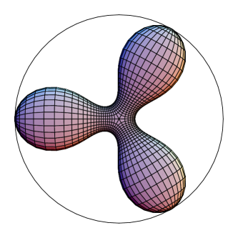
(a) $d_{0}<D_{0}$

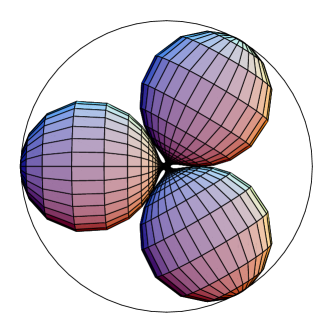
(b) $d_{0}=0,2332\approx D_{0}$

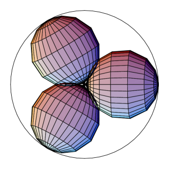
(c) $d_{0}=0,2400$

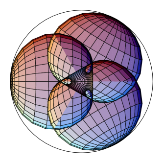
(d) $d_{0}>D_{0}$

Fig. 3: Symmetric trinoids

The CMC-1 trinoids build a three-parameter family. Indeed, let us fix the points on the absolute applying isometries of $\mathbb{H}^{3}$. We fix the images of the ends $z_{j},j=0,1,\infty$ at the points $(-\tfrac{1}{2},0,-\tfrac{\sqrt{3}}{2})$, $(1,0,0)$ and $(-\tfrac{1}{2},0,\tfrac{\sqrt{3}}{2})$ respectively. This implies the following relations between the parameters $p_{0},p_{1},p_{\infty},q_{0},q_{1},q_{\infty}$:

$$p_{0}= (2-\sqrt{3})q_{0},$$ (7.5)

$$p_{1}= -q_{1},$$

$$p_{\infty}= (2+\sqrt{3})q_{\infty}.$$

Two embedded examples are shown in Fig. 1 in the introduction.

The condition $d_{0}=d_{1}=d_{\infty}$ characterizes the symmetric trinoids. They build a one-parameter family characterized by the parameter $d_{0}$. There is $D_{0}<\tfrac{1}{4}$ such that all symmetric trinoids with $d_{0}<D_{0}$ are embedded and all trinoids with $d_{0}>D_{0}$ are not embedded, see Fig. 3.

Fig. 4: Parameter lines in the $z$-plane

Figs. 1 and 3 were produced using the software Mathematica, which provides an implementation of the hypergeometric function. The parameterization in these figures was chosen to show the umbilic points at the centers of both sides of the symmetric trinoids. We split the complex $z$-plane in three domains associated to the ends and use the following parameterization for these domains

$$z=\begin{cases}z(w_{0}),&\text{for end $z=0$},\\ z(w_{1}),&\text{for end $z=1$},\\ z(w_{\infty}),&\text{for end $z=\infty$}\end{cases}\quad z(w_{j})=\frac{z_{1}-z_{\infty}}{z_{1}-z_{0}}\frac{w_{j}-z_{0}}{w_{j}-z_{\infty}},$$

where $w_{j}=(-\frac{\tilde{w}+1}{\tilde{w}-1})^{\tfrac{2}{3}}z_{j}$, $z_{0}=e^{i\tfrac{\pi}{6}}$, $z_{1}=e^{i\tfrac{5\pi}{6}}$, $z_{\infty}=e^{i\tfrac{3\pi}{2}}$, $|\tilde{w}|\leq 1$. The corresponding parameter lines $w\in\mathbb{R}$, $w\in i\mathbb{R}$ in the $z$-plane are shown in Fig. 4.

The Mathematica notebook as well as additional images of trinoids can be found from the URL http://www-sfb288.math.tu-berlin.de/~bobenko

Acknowledgment We are grateful to Alexander Its for a useful correspondence and for showing his formulas on integration of Fuchsian systems with three singularities in hypergeometric functions prior to publication of his book. This research was financially supported by Deutsche Forschungsgemeinschaft (SFB 288 ”Differential Geometry and Quantum Physics”).

Appendix A Basic facts about the hypergeometric function

We present some facts about the hypergeometric function used in the proofs of Theorem 4 and Lemma 2.

The function represented by the infinite series $\overset{{}^{\infty}}{\underset{n=0}{\sum}}\frac{(a)_{n}\,(b)_{n}}{(c)_{n}}\,\frac{z^{n}}{n!}$ within its circle of convergence and its analytic continuation is called the hypergeometric function ${{}_{2}F_{1}}(a,b;c;z)$. The symbol $(a)_{n}$ is defined as

$$(a)_{n}\,=\,a(a+1)(a+2)\dotsb(a+n-1)\,=\,\frac{\Gamma(a+n)}{\Gamma(a)}\,.$$

Thus

$${{}_{2}F_{1}}(a,b;c;z)\,=\,\frac{\Gamma(c)}{\Gamma(a)\,\Gamma(b)}\,\sum_{n=0}^{\infty}\frac{\Gamma(a+n)\,\Gamma(b+n)}{\Gamma(c+n)}\frac{z^{n}}{n!}\,.$$

For later use we give some formulas for hypergeometric functions [MOS, Er, WW].

Differentiation formula.

$$\frac{d^{n}}{dz^{n}}\,{{}_{2}F_{1}}(a,b;c;z)\,=\,\frac{(a)_{n}\,(b)_{n}}{(c)_{n}}\,{{}_{2}F_{1}}(a+n,b+n;c+n;z)\,.$$

Gauss’ contiguous relations.

The six functions

$${{}_{2}F_{1}}(a\pm 1,b;c;z),\quad{{}_{2}F_{1}}(a,b\pm 1;c;z),\quad{{}_{2}F_{1}}(a,b;c\pm 1;z)$$

are called contiguous to ${{}_{2}F_{1}}(a,b;c;z)$. A relation between ${{}_{2}F_{1}}(a,b;c;z)$ and any two contiguous functions is called a contiguous relation. By these relations, one can expresses the function ${{}_{2}F_{1}}(a+l,b+m;c+n;z)$ with $l,m,n\in\mathbb{Z}$, $c+n\neq 0,\,-1,\,-2,\,\dotsc$ as a linear combination of ${{}_{2}F_{1}}(a,b;c;z)$ and one of its contiguous functions. The coefficients are rational functions of $a,\,b,\,c,\,z$. For example, one has the following formulas:

$${{}_{2}F_{1}}(a+1,b+1;c+1;z)\,=\,\frac{1}{a\,b\,(1-z)}\,\\ \left[c\,(a+b-c)\;{{}_{2}F_{1}}(a,b;c;z)+(c-a)\,(c-b)\;{{}_{2}F_{1}}(a,b;c+1;z)\right]\,,$$ (A.1)

$${{}_{2}F_{1}}(a+1,b+1;c+2;z)\,=\,\\ \frac{c\,(c+1)}{a\,b\,z}\,\left[{{}_{2}F_{1}}(a,b;c;z)-{{}_{2}F_{1}}(a,b;c+1;z)\right]\,.$$ (A.2)

The connection between hypergeometric functions of $z$ and of $1-z$.

For $|\arg(1-z)|<\pi$ and $c-a-b\not\in\{0,\pm 1,\pm 2,\dotsc\}$,

$${{}_{2}F_{1}}(a,b;c;z)=\\ \frac{\Gamma(c)\Gamma(c-a-b)}{\Gamma(c-a)\Gamma(c-b)}{{}_{2}F_{1}}(a,b;a+b-c+1;1-z)+\\ (1-z)^{c-a-b}\frac{\Gamma(c)\Gamma(a+b-c)}{\Gamma(a)\Gamma(b)}{{}_{2}F_{1}}(c-a,c-b;c-a-b+1;1-z).$$ (A.3)

The hypergeometric differential equation

$$z\,(1-z)\,\frac{d^{2}w}{dz^{2}}+[c-(a+b+1)\,z]\,\frac{dw}{dz}-a\,b\,w\,=\,0$$ (A.4)

has three regular singular points $z=0,\,1,\,\infty$. The pairs of characteristic exponents at these points are

$$\rho_{0}\, =\,0\,, \quad\rho_{1}\, =\,0\,, \quad\rho_{\infty}\, =\,a\,,$$

$$\rho_{0}^{\prime}\, =\,1-c\,, \quad\rho_{1}^{\prime}\, =\,c-a-b\,, \quad\rho_{\infty}^{\prime}\, =\,b$$

respectively. The hypergeometric function ${{}_{2}F_{1}}(a,b;c;z)$ is a solution of the hypergeometric differential equation which is unbranched at $z=0$.

Proposition 3 ([Kl]).

The fundamental system of linearly independent solutions of hypergeometric differential equation (A.4) at the singular points $z=0,1,\infty$ is given by

$$w_{1}^{(0)}(z)\, =\,{{}_{2}F_{1}}(a,b;c;z)\,,$$

$$w_{2}^{(0)}(z)\, =\,z^{1-c}\,{{}_{2}F_{1}}(a-c+1,b-c+1;2-c;z)\,,$$

$$w_{1}^{(1)}(z)\, =\,{{}_{2}F_{1}}(a,b;a+b-c+1;1-z)\,,$$

$$w_{2}^{(1)}(z)\, =\,(1-z)^{c-a-b}\,{{}_{2}F_{1}}(c-b,c-a;c-a-b+1;1-z)\,,$$

$$w_{1}^{(\infty)}(z)\, =\,z^{-a}\,{{}_{2}F_{1}}(a,a-c+1;a-b+1;\frac{1}{z})\,,$$

$$w_{2}^{(\infty)}(z)\, =\,z^{-b}\,{{}_{2}F_{1}}(b,b-c+1;b-a+1;\frac{1}{z})\,.$$

Riemann’s differential equation.

The hypergeometric differential equation is a special case of Riemann’s differential equation

$$\frac{d^{2}w}{dz^{2}}+\left[\frac{1-\rho_{a}-\rho_{a}^{\prime}}{z-a}+\frac{1-\rho_{b}-\rho_{b}^{\prime}}{z-b}+\frac{1-\rho_{c}-\rho_{c}^{\prime}}{z-c}\right]\,\frac{dw}{dz}\\ +\left[\frac{\rho_{a}\,\rho_{a}^{\prime}\,(a-b)\,(a-c)}{z-a}+\frac{\rho_{b}\,\rho_{b}^{\prime}\,(b-c)\,(b-a)}{z-b}+\frac{\rho_{c}\,\rho_{c}^{\prime}\,(c-a)\,(c-b)}{z-c}\right]\\ \times\frac{w}{(z-a)\,(z-b)\,(z-c)}\,=\,0\,.$$

The characteristic exponents $\rho_{a}$, ${\rho_{a}}^{\prime}$; ${\rho_{b}}$, ${\rho_{b}}^{\prime}$; $\rho_{c}$, ${\rho_{c}}^{\prime}$ must satisfy the additional relation

$$\sum_{j=0,1,\infty}\,(\rho_{j}+{\rho_{j}}^{\prime})=1.$$

The following symbol is used for Riemann’s differential equation:

$$P\left\{\begin{matrix}a&b&c&\\ \rho_{a}&\rho_{b}&\rho_{c}&;z\\ \rho_{a}^{\prime}&\rho_{b}^{\prime}&\rho_{c}^{\prime}&\end{matrix}\right\}\,.$$

It is also used to denote the set of solutions of the equation and called Riemann P-function.

In particular, the hypergeometric differential equation (A.4) is

$$P\left\{\begin{matrix}0&\infty&1&\\ 0&a&0&;z\\ 1-c&b&c-a-b&\end{matrix}\right\}\,.$$

The generalized hypergeometric differential equation

$$\frac{d^{2}w}{dz^{2}}+\left[\frac{1-\rho_{0}-\rho_{0}^{\prime}}{z}+\frac{1-\rho_{1}-\rho_{1}^{\prime}}{z-1}\right]\,\frac{dw}{dz}\\ +\left[\frac{-\rho_{0}\,\rho_{0}^{\prime}}{z}+\frac{\rho_{1}\,\rho_{1}^{\prime}}{z-1}+\rho_{\infty}\,\rho_{\infty}^{\prime}\right]\,\frac{w}{z\,(z-1)}\,=\,0$$ (A.5)

is represented by

$$P\left\{\begin{matrix}0&\infty&1&\\ \rho_{0}&\rho_{\infty}&\rho_{1}&;z\\ \rho_{0}^{\prime}&\rho_{\infty}^{\prime}&\rho_{1}^{\prime}&\end{matrix}\right\}\,.$$

The following two transformations formulas are valid for Riemann’s $P$-function

$$1.\quad P\left\{\begin{matrix}0&\infty&1&\\ \rho_{0}&\rho_{\infty}&\rho_{1}&;z\\ \rho_{0}^{\prime}&\rho_{\infty}^{\prime}&\rho_{1}^{\prime}&\end{matrix}\right\}\\ =\,z^{-k}\,(z-1)^{-l}\,P\left\{\begin{matrix}0&\infty&1&\\ \rho_{0}+k&\rho_{\infty}-k-l&\rho_{1}+l&;z\\ \rho_{0}^{\prime}+k&\rho_{\infty}^{\prime}-k-l&\rho_{1}^{\prime}+l&\end{matrix}\right\}\,;\\ 2a.\quad P\left\{\begin{matrix}0&\infty&1&\\ \rho_{0}&\rho_{\infty}&\rho_{1}&;z\\ \rho_{0}^{\prime}&\rho_{\infty}^{\prime}&\rho_{1}^{\prime}&\end{matrix}\right\}\,=\,P\left\{\begin{matrix}1&\infty&0&\\ \rho_{0}&\rho_{\infty}&\rho_{1}&;1-z\\ \rho_{0}^{\prime}&\rho_{\infty}^{\prime}&\rho_{1}^{\prime}&\end{matrix}\right\}\,;\\ 2b.\quad P\left\{\begin{matrix}0&\infty&1&\\ \rho_{0}&\rho_{\infty}&\rho_{1}&;z\\ \rho_{0}^{\prime}&\rho_{\infty}^{\prime}&\rho_{1}^{\prime}&\end{matrix}\right\}\,=\,P\left\{\begin{matrix}\infty&0&1&\\ \rho_{0}&\rho_{\infty}&\rho_{1}&;\frac{1}{z}\\ \rho_{0}^{\prime}&\rho_{\infty}^{\prime}&\rho_{1}^{\prime}&\end{matrix}\right\}\,.\hfill$$

Proposition 4.

The fundamental system of linear independent solutions of generalized hypergeometric equation (A.5) at the singular points $z=0,\,1,\,\infty$ is given by

$$w_{1}^{(0)}(z)\, =\,z^{\rho_{0}}\,(z-1)^{\rho_{1}}\,{{}_{2}F_{1}}(a,b;c;z)\,,$$

$$w_{2}^{(0)}(z)\, =\,z^{\rho_{0}^{\prime}}\,(z-1)^{\rho_{1}}\,{{}_{2}F_{1}}(a-c+1,b-c+1;2-c;z)\,,$$

$$w_{1}^{(1)}(z)\, =\,z^{\rho_{0}}\,(z-1)^{\rho_{1}}\,{{}_{2}F_{1}}(a,b;a+b-c+1;1-z)\,,$$

$$w_{2}^{(1)}(z)\, =\,z^{\rho_{0}}\,(z-1)^{\rho_{1}^{\prime}}\,{{}_{2}F_{1}}(c-b,c-a;c-a-b+1;1-z)\,,$$

$$w_{1}^{(\infty)}(z)\, =\,z^{-\rho_{1}-\rho_{\infty}}\,(z-1)^{\rho_{1}}\,{{}_{2}F_{1}}(a,a-c+1;a-b+1;\frac{1}{z})\,,$$

$$w_{2}^{(\infty)}(z)\, =\,z^{-\rho_{1}-\rho_{\infty}^{\prime}}\,(z-1)^{\rho_{1}}\,{{}_{2}F_{1}}(b,b-c+1;b-a+1;\frac{1}{z})\,,$$

where

$$a\,=\,\rho_{0}+\rho_{1}+\rho_{\infty}\,,\quad b\,=\,\rho_{0}+\rho_{1}+\rho_{\infty}^{\prime}\,,\quad c\,=\,1+\rho_{0}-\rho_{0}^{\prime}\,.$$

Appendix B The proofs of Theorem 4 and Lemma 2

Proof of Theorem 4.

Reduce the Fuchsian system (5.5)

$$\begin{pmatrix}\varphi_{11}^{\prime}&\varphi_{12}^{\prime}\\ \varphi_{21}^{\prime}&\varphi_{22}^{\prime}\end{pmatrix}\, =\,\begin{pmatrix}\frac{\alpha}{z}+\frac{\beta}{z-1}&\frac{\gamma}{z-1}\\ \frac{\varepsilon^{2}\,\delta}{z-1}&-\frac{\alpha}{z}-\frac{\beta}{z-1}\end{pmatrix}\cdot\begin{pmatrix}\varphi_{11}&\varphi_{12}\\ \varphi_{21}&\varphi_{22}\end{pmatrix}\,$$

$$=\,\begin{pmatrix}a_{11}&a_{12}\\ a_{21}&a_{22}\end{pmatrix}\cdot\begin{pmatrix}\varphi_{11}&\varphi_{12}\\ \varphi_{21}&\varphi_{22}\end{pmatrix}$$

to the following system of second-order differential equations.

$$\left\{\begin{minipage}[c]{420.61192pt} \@@amsalign\varphi_{1j}^{\prime}&=a_{11}\varphi_{1j}+a_{12}\varphi_{2j},\quad j=1,2\\ \varphi_{2j}^{\prime}&=a_{21}\varphi_{1j}+a_{22}\varphi_{2j},\quad j=1,2\\ \varphi_{1j}^{\prime\prime}&=\varphi_{1j}^{\prime}\left(a_{11}+a_{22}+\tfrac{a_{12}^{\prime}}{a_{12}}\right)+\varphi_{1j}\left(a_{12}a_{21}-a_{11}a_{22}+\tfrac{a_{11}^{\prime}a_{12}-a_{11}a_{12}^{\prime}}{a_{12}}\right)\\ &=\varphi_{1j}^{\prime}\left(-\tfrac{1}{z-1}\right)+\varphi_{1j}\left(\tfrac{\alpha^{2}-\alpha}{z^{2}}+\tfrac{\beta^{2}+\gamma\delta}{(z-1)^{2}}+\tfrac{\alpha(2\beta+1)}{z(z-1)}\right),\quad j=1,2\\ \varphi_{2j}^{\prime\prime}&=\varphi_{2j}^{\prime}\left(a_{11}+a_{22}+\tfrac{a_{21}^{\prime}}{a_{21}}\right)+\varphi_{2j}\left(a_{12}a_{21}-a_{11}a_{22}+\tfrac{a_{22}^{\prime}a_{21}-a_{22}a_{21}^{\prime}}{a_{21}}\right)\\ &=\varphi_{2j}^{\prime}\left(-\tfrac{1}{z-1}\right)+\varphi_{2j}\left(\tfrac{\alpha^{2}+\alpha}{z^{2}}+\tfrac{\beta^{2}+\gamma\delta}{(z-1)^{2}}+\tfrac{\alpha(2\beta-1)}{z(z-1)}\right),\quad j=1,2. \end{minipage}\right.$$

Equations (B.3), (B.4) are the generalized hypergeometric differential equations with the characteristic exponents

$$\rho_{0}\, =\,\alpha\,, \quad\rho_{1}\, =\,\sqrt{\beta^{2}+\gamma\,\delta}\,, \quad\rho_{\infty}\, =\,\sqrt{(\alpha+\beta)^{2}+\gamma\,\delta}\,,$$

$$\rho_{0}^{\prime}\, =\,1-\alpha\,, \quad\rho_{1}^{\prime}\, =\,-\sqrt{\beta^{2}+\gamma\,\delta}\,, \quad\rho_{\infty}^{\prime}\, =\,-\sqrt{(\alpha+\beta)^{2}+\gamma\,\delta}$$

and

$$\widetilde{\rho}_{0}\, =\,1+\alpha\,, \quad\widetilde{\rho}_{1}\, =\,\sqrt{\beta^{2}+\gamma\,\delta}\,, \quad\widetilde{\rho}_{\infty}\, =\,\sqrt{(\alpha+\beta)^{2}+\gamma\,\delta}\,,$$

$$\widetilde{\rho}_{0}^{\prime}\, =\,-\alpha\,, \quad\widetilde{\rho}_{1}^{\prime}\, =\,-\sqrt{\beta^{2}+\gamma\,\delta}\,, \quad\widetilde{\rho}_{\infty}^{\prime}\, =\,-\sqrt{(\alpha+\beta)^{2}+\gamma\,\delta}$$

respectively. Chose the ansatz

$$\Phi^{(0)}(z)\,=\,\begin{pmatrix}k_{11}\,w_{1}^{(0)}(z)&w_{2}^{(0)}(z)\\ \widetilde{w}_{1}^{(0)}(z)&k_{22}\,\widetilde{w}_{2}^{(0)}(z)\end{pmatrix}\,,$$

for a solution of the Fuchsian system at $z=0$. Here, $w_{1}^{(0)}(z),\,w_{2}^{(0)}(z)$ and $\widetilde{w}_{1}^{(0)}(z),\,\widetilde{w}_{2}^{(0)}(z)$ are linearly independent solutions of equations (B.3) and (B.4), respectively. Due to Proposition 4, the function $w_{1}^{(0)}(z)$, $w_{2}^{(0)}(z)$, $\widetilde{w}_{1}^{(0)}(z)$, $\widetilde{w}_{2}^{(0)}(z)$ can be chosen as follows:

$$w_{1}^{(0)}(z) =\,z^{\alpha}\,(z-1)^{\tau}\,{{}_{2}F_{1}}(a,b;c;z)\,,$$

$$w_{2}^{(0)}(z) =\,z^{1-\alpha}\,(z-1)^{\tau}\,{{}_{2}F_{1}}(a-c+1,b-c+1;2-c;z)\,,$$

$$\widetilde{w}_{1}^{(0)}(z) =\,z^{1+\alpha}\,(z-1)^{\tau}\,{{}_{2}F_{1}}(a+1,b+1;c+2;z)\,,$$

$$\widetilde{w}_{2}^{(0)}(z) =\,z^{-\alpha}\,(z-1)^{\tau}\,{{}_{2}F_{1}}(a-c,b-c;-c;z)\,,$$

where

$$a\, =\,\rho_{0}+\rho_{1}+\rho_{\infty}\,=\,\alpha+\tau+\rho\,,$$

$$b\, =\,\rho_{0}+\rho_{1}+\rho_{\infty}^{\prime}\,=\,\alpha+\tau-\rho\,,$$

$$c\, =\,1+\rho_{0}-\rho_{0}^{\prime}\,=\,2\alpha\,,$$

$$\widetilde{a}\, =\,\widetilde{\rho}_{0}+\widetilde{\rho}_{1}+\widetilde{\rho}_{\infty}\,=\,1+\alpha+\tau+\rho\,=\,a+1,$$

$$\widetilde{b}\, =\,\widetilde{\rho}_{0}+\widetilde{\rho}_{1}+\widetilde{\rho}_{\infty}^{\prime}\,=\,1+\alpha+\tau-\rho\,=\,b+1,$$

$$\widetilde{c}\, =\,1+\widetilde{\rho}_{0}-\widetilde{\rho}_{0}^{\prime}\,=\,2+2\alpha\,=\,c+2\,.$$

The coefficients $k_{11},\,k_{22}$ follow from the conditions (B.1), (B.2):

$$k_{11}\,\frac{d}{dz}w_{1}^{(0)}(z)-a_{11}\,k_{11}\,w_{1}^{(0)}(z)-a_{12}\,k_{21}\,\widetilde{w}_{1}^{(0)}(z)\,=\\ z^{\alpha}\,(z-1)^{\tau-1}\,\biggl{[}-\gamma\,z\,{{}_{2}F_{1}}(a+1,b+1;c+2,z)\biggr{.}\\ \biggl{.}+k_{11}\,\biggl{(}(\tau-\beta)\,{{}_{2}F_{1}}(a,b;c,z)+\frac{a\,b}{c}\,(z-1)\,{{}_{2}F_{1}}(a+1,b+1;c+1,z)\biggr{)}\biggr{]}\overset{\eqref{ReduceGauss1},\eqref{ReduceGauss2}}{=}\,\\ z^{\alpha}\,(z-1)^{\tau-1}\,\biggl{[}-\gamma\,\frac{c\,(c+1)}{a\,b}\,\biggl{(}{{}_{2}F_{1}}(a,b;c,z)-{{}_{2}F_{1}}(a,b;c+1,z)\biggr{)}\biggr{.}\\ \biggl{.}+k_{11}\,\biggl{(}(\tau-\beta+a+b-c)\,{{}_{2}F_{1}}(a,b;c,z)-\frac{(c-a)\,(c-b)}{c}\,{{}_{2}F_{1}}(a,b;c+1;z)\biggr{)}\biggr{]}\,=\\ z^{\alpha}\,(z-1)^{\tau-1}\,\biggl{[}\frac{\gamma\,(2\alpha+1)}{\tau-\beta}\,\biggl{(}{{}_{2}F_{1}}(a,b;c+1;z)-{{}_{2}F_{1}}(a,b;c,z)\biggr{)}\biggr{.}\\ \biggl{.}+k_{11}\,(\tau+\beta)\,\biggl{(}{{}_{2}F_{1}}(a,b;c+1;z)-{{}_{2}F_{1}}(a,b;c,z)\biggr{)}\biggr{]}\,=\,0.$$

Hence, $k_{11}\,=\,-\frac{2\alpha+1}{\delta}$. The formula for $k_{22}$ is obtained analogously.

From Proposition 4 we know the system of two linear independent solutions for the equations (B.3), (B.4) both in the neighborhood of $z=1$ and of $z=\infty$. In the same way as for the canonical solution $\Phi^{(0)}(z)$ we prove the formulas for $\Phi^{(1)}(z)$ and $\Phi^{(\infty)}(z)$. ∎

Proof of Lemma 2.

Let us compute the connection matrix $E_{1}$. Using the representations (6.5) and (6.6) for $\Phi^{(0)}(z)$ and $\Phi^{(1)}(z)$ we have

$$\Phi_{11}^{(1)}(z)\,E_{1}^{11}+\Phi_{12}^{(1)}(z)\,E_{1}^{21}\\ =\frac{\beta+\tau}{\delta}\,z^{\alpha}\,(z-1)^{\tau}\,{{}_{2}F_{1}}(a,b;a+b-c+1;1-z)\,E_{1}^{11}\\ +z^{\alpha}\,(z-1)^{-\tau}\,{{}_{2}F_{1}}(c-a,c-b;c-a-b+1;1-z)\,E_{1}^{21}\\ =\,\Phi_{11}^{(0)}(z)\,=\,-\frac{2\alpha+1}{\delta}z^{\alpha}\,(z-1)^{\tau}\,{{}_{2}F_{1}}(a,b;c;z)\\ \overset{(\ref{connect0_1})}{=}\,-\frac{2\alpha+1}{\delta}z^{\alpha}\,(z-1)^{\tau}\,\left[\frac{\Gamma(c)\,\Gamma(c-a-b)}{\Gamma(c-a)\,\Gamma(c-b)}\,{{}_{2}F_{1}}(a,b;a+b-c+1;1-z)\right.\\ \left.+(1-z)^{c-a-b}\,\frac{\Gamma(c)\,\Gamma(a+b-c)}{\Gamma(a)\,\Gamma(b)}\,{{}_{2}F_{1}}(c-a,c-b;c-a-b+1;1-z)\right]\\ =\,-\frac{2\alpha+1}{\delta}\,\frac{\Gamma(c)\,\Gamma(c-a-b)}{\Gamma(c-a)\,\Gamma(c-b)}\,z^{\alpha}\,(z-1)^{\tau}\,{{}_{2}F_{1}}(a,b;a+b-c+1;1-z)\\ -\frac{2\alpha+1}{\delta}\,\frac{\Gamma(c)\,\Gamma(a+b-c)}{\Gamma(a)\,\Gamma(b)}\,z^{\alpha}(z-1)^{\tau}(1-z)^{-2\tau}\,{{}_{2}F_{1}}(c-a,c-b;c-a-b+1;1-z)\,,$$ (B.6)

since Theorem 4 implies $c-a-b=-2\,\tau$.

Here the branches of $z$ and $(z-1)$ are fixed by $0<\arg z<2\pi$ and $0<\arg(z-1)<2\pi$. Using

$$(z-1)^{\tau}(1-z)^{-2\tau}=(z-1)^{-\tau}e^{2\tau\pi i}$$

and identifying the coefficients at the hypergeometric functions in (B.6) we obtain

$$E_{1}^{11}\, =\,-\frac{2\alpha+1}{\beta+\tau}\,\frac{\Gamma(c)\Gamma(c-a-b)}{\Gamma(c-a)\Gamma(c-b)},$$

$$E_{1}^{21}\, =\,-\frac{2\alpha+1}{\delta}\,\frac{\Gamma(c)\Gamma(a+b-c)}{\Gamma(a)\Gamma(b)}e^{2\tau\pi i}.$$

It is easy to verify that the equality

$$\Phi_{21}^{(0)}(z)\,=\,\Phi_{21}^{(1)}(z)\,E_{1}^{11}+\Phi_{22}^{(1)}(z)\,E_{1}^{21}$$

also holds. Similarly we can obtain the formulas for $E_{1}^{12}$ and $E_{1}^{22}$. The computation for $E_{\infty}$ is analogous. ∎

References

[Bi]
I. Biswas, A criterion for the existence of a parabolic stable
bundle of rank two over the projective line, Int. Journal of
Math. 9:5 (1998), 523-533
[Bo]
A.I. Bobenko, Surfaces in terms of by matrices. Old and
new integrable cases, In: A. Fordy, J. Wood (eds.), Harmonic
maps and integrable systems, Vieweg, Brauschweig, 1994, pp.
83-127
[Br]
R.L. Bryant, Surfaces of mean curvature one in hyperbolic space,
Astérisque, 154-155 (1987), 321-347
[CHR]
P. Collin, L. Hauswirth, H. Rosenberg, The geometry of finite
topology Bryant surfaces, Ann. of Math. (2), 153(3)
(2001), 623-659
[Er]
A. Erdélyi, W. Magnus, F. Oberhettinger, F.G. Tricomi, Higher transcendental functions. Vol. I, McGraw-Hill
Book Co., New York, 1953
[Kl]
F. Klein, Vorlesungen über die hypergeometrische
Funktion, Springer-Verlag, Berlin, 1981. Reprint of the 1933
original
[KS]
R. Kusner, N. Schmitt, The spinor representation of surfaces in
space, arXiv:dg-ga/9610005, (1996)
[MOS]
W. Magnus, F. Oberhettinger and R. P. Soni, Formulas and
theorems for the special functions of mathematical physics,
Springer-Verlag, Berlin, 1966
[RUY]
W. Rossman, M. Umehara, K. Yamada, Irreducible constant mean
curvature 1 surfaces in hyperbolic space with positive genus, Tôhoku Math. J., 49 (1997), 449-484
[UY93]
M. Umehara, K. Yamada, Complete surfaces of constant mean
curvature-1 in the hyperbolic 3-space, Ann. of Math., 137 (1993), 611-638
[UY96]
M. Umehara, K. Yamada, Surfaces of constant mean curvature in
with prescribed hyperbolic Gauss map, Math. Ann.,
304(2) (1996), 203-209
[UY96]
M. Umehara, K. Yamada, Metrics of constant curvature 1 with three
conical singularities on the 2-sphere, Illinois J. Math.,
44(1) (2000), 72-94
[WW]
E.T. Whittaker, G.N. Watson, A course of modern analysis,
Cambridge University Press, Cambridge 1962