How to sum up triangles

Abstract

We prove configuration theorems that generalize the Desargues, Pascal, and Pappus theorems. Our generalization of the Desargues theorem allows us to introduce the structure of an Abelian group on the (properly extended) set of triangles which are perspective from a point. In barycentric coordinates, the corresponding group operation becomes the addition in $\mathbb{R}^{3}$.

Keywords: configuration theorems, projective plane, additive group of triangles, barycentric coordinates

MSC: 51A20, 51A30, 51E15

1 Configuration theorems

1.1 The Desargues theorem and its generalization

In this paper we deal with points and (straight) lines on the (real projective) plane. By a configuration we understand a set of points and lines on this plane.

Definition 1.1.

If there is a correspondence between two configurations such that all the lines passing through the corresponding points meet in a point $O$, then we say that these configurations are perspective from the point $O$ and we call $O$ the perspective center.

If there is a correspondence between two configurations such that all the intersection points of the corresponding lines lie on a line $\ell$, then we say that these configurations are perspective from the line $\ell$ and we call $\ell$ the perspective axis.

Theorem (Desargues).

If two triangles are perspective from a point, they are also perspective from a line.

The converse (also referred to as the “dual”) Desargues theorem holds as well: if two triangles are perspective from a line, then they are perspective from a point.

An interested reader can find a proof of the Desargues theorem in the books [1], [2], [4].

Thus, the Desargues theorem states that the intersection points of the corresponding sides of two perspective triangles lie on a line. Can we say anything about the intersection points of non-corresponding sides? It turns out that we can!

Definition 1.2 (The main construction).

Let $A_{1}A_{2}A_{3}$ and $B_{1}B_{2}B_{3}$ be triangles perspective from a point $S$. Let $(i,j,k)$ stand for a permutation of the numbers 1, 2, 3. Let $P_{ij}$ be the intersection point of the lines $A_{i}A_{k}$ and $B_{j}B_{k}$. We denote $S_{k}=A_{i}A_{j}\cap B_{i}B_{j}$ and $C_{k}=P_{ik}P_{ki}\cap P_{jk}P_{kj}$ (see fig. 1).

Theorem 1.1 (Generalized Desargues theorem).

The triangle $C_{1}C_{2}C_{3}$ is perspective to the triangles $A_{1}A_{2}A_{3}$ and $B_{1}B_{2}B_{3}$ from the point $S$.

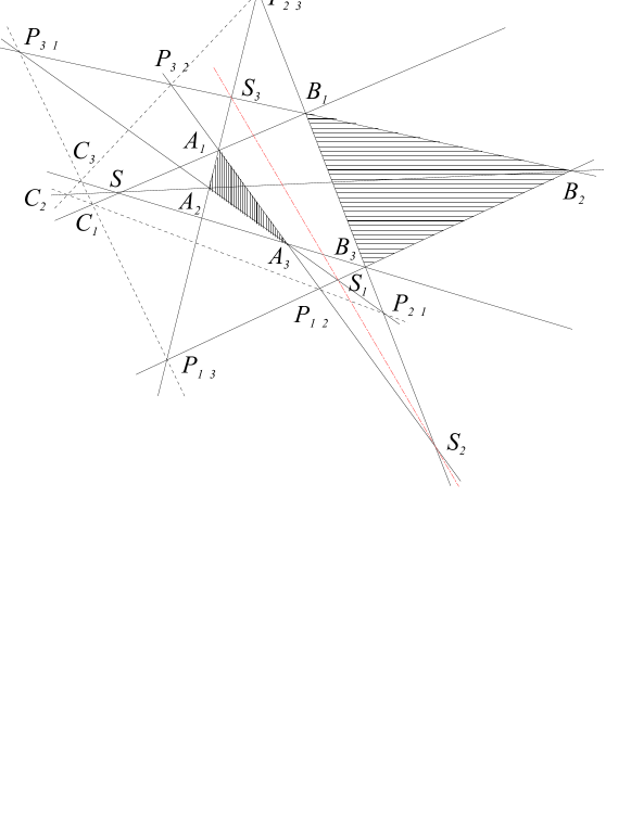
Figure 1: Desargues theorem and its generalization

We will give two proofs of this theorem.

Proof 1.

Let us check that the triangles $\Delta_{1}=S_{1}P_{21}P_{12}$ and $\Delta_{2}=S_{3}P_{23}P_{32}$ are perspective from the point $S_{2}$. For this purpose we will show that the lines $P_{21}P_{23}$, $P_{12}P_{32}$, and $S_{1}S_{3}$ pass through the point $S_{2}$. Observe that $P_{21}P_{23}$ is actually the line $B_{3}B_{1}$ and that $P_{12}P_{32}$ is actually the line $A_{1}A_{3}$. Therefore these two lines intersect in the point $S_{2}$. It remains to notice that $S_{1}$, $S_{2}$, and $S_{3}$ are collinear by an application of the Desargues theorem to the triangles $A_{1}A_{2}A_{3}$ and $B_{1}B_{2}B_{3}$.

Thus, the triangles $\Delta_{1}$ and $\Delta_{2}$ are perspective from a point. Hence, by the Desargues theorem, the intersection points of the corresponding sides,

$$A_{2} =S_{1}P_{21}\cap S_{3}P_{23},$$

$$B_{2} =S_{1}P_{12}\cap S_{3}P_{32},$$

$$C_{2} =P_{21}P_{12}\cap P_{23}P_{32},$$

are collinear. Analogously, $C_{1}\in A_{1}B_{1}$, $C_{3}\in A_{3}B_{3}$, which completes the proof. ∎

Proof 2.

We will need the following fact about algebraic curves (see [3], chapter 1, § 1, Theorem 4 for $n=4$):

Let $A_{ij}$ be (pairwise distinct) intersection points of lines $p_{i}$, $q_{j}$, $1\leqslant i,j\leqslant 4$. If all the following points

$$\begin{array}[]{cccc}A_{11},&A_{12},&A_{13},&A_{14},\\ A_{21},&A_{22},&A_{23},&A_{24},\\ A_{31},&A_{32},&A_{33},\\ A_{41},&A_{42}\\ \end{array}$$

belong to an algebraic curve of degree four, then the remaining points $A_{34}$, $A_{43}$, $A_{44}$ belong to this curve as well.

Consider the triangles $A_{1}A_{2}A_{3}$ and $B_{1}B_{2}B_{3}$ that are perspective from the point $S$. Construct the points $P_{ij}$. Define the points $C_{i}$ not as in the main configuration but as follows: $C_{1}^{\prime}=P_{12}P_{21}\cap A_{1}B_{1}$, $C_{2}^{\prime}=P_{12}P_{21}\cap P_{23}P_{32}$, $C_{3}^{\prime}=P_{23}P_{32}\cap A_{3}B_{3}$. Let us denote straight lines in an over-determined way by listing those points of the obtained configuration which belong to these lines. Consider the lines

$$p_{1} =P_{23}A_{1}A_{2}P_{13}, q_{1} =P_{31}A_{2}A_{3}P_{21}, r_{1} =P_{31}P_{13},$$

$$p_{2} =P_{31}P_{32}B_{1}B_{2}, q_{2} =P_{13}P_{12}B_{3}B_{2}, r_{2} =P_{32}A_{1}A_{3}P_{12},$$

$$p_{3} =C_{3}^{\prime}SA_{3}B_{3}, q_{3} =C_{1}^{\prime}SA_{1}B_{1}, r_{3} =P_{23}B_{1}B_{3}P_{21},$$

$$p_{4} =C_{2}^{\prime}C_{1}^{\prime}P_{12}P_{21}, q_{4} =C_{2}^{\prime}C_{3}^{\prime}P_{32}P_{23}, r_{4} =SA_{2}B_{2}.$$

We see that the intersection points of $p_{i}$ and $q_{i}$ give 16 points of our configuration. All of them, except maybe $C_{1}^{\prime}$, $C_{2}^{\prime}$, and $C_{3}^{\prime}$, belong to a curve of degree four that is the union of the four lines $r_{1}$, $r_{2}$, $r_{3}$, and $r_{4}$. In the notations of the above mentioned theorem from [3] we have $C_{1}^{\prime}=A_{43}$, $C_{2}^{\prime}=A_{44}$, $C_{3}^{\prime}=A_{34}$. Therefore, these points must also belong to the union of the lines $r_{i}$. It is easy to check that none of the lines $r_{i}$ contains five points of our configuration. Hence the points $C_{3}^{\prime}$ and $C_{1}^{\prime}$ lie on $r_{1}$; and the point $C_{2}^{\prime}$ lies on $r_{4}$. This completes the proof. ∎

In the book [2] (§ 22), the Reye configuration with parameters (12, 4, 16, 3) is described. The vertices of the configuration are the vertices of a cube, its center, and three points at infinity which correspond to the directions of the edges of the cube. The lines of the configuration are the edges and the four main diagonals of the cube. It is not difficult to verify that the configuration described in Theorem 1.1 is dual to the Reye configuration.

Remark. The Pascal theorem can be proven by similar considerations. In fact, it is a theorem on associativity of the addition operation for points on an elliptic curve. Unfortunately our theorem 1.1 does not seem to be associated with any operation for objects related to a curve of degree four. We do not have even a configuration theorem for a generic curve of degree four.

1.2 The Pappus and Pascal theorems

In this subsection we will prove generalizations of the Pappus and Pascal theorems. Readers familiar with the polar transform and dual theorems can easily generalize the Brianchon theorem along the same lines.

Theorem (Pascal).

If a simple hexagon is inscribed in a conic section, then the three intersection points of opposite sides of the hexagon are collinear.

Theorem (Pappus).

Let the points $A_{1}$, $A_{2}$, $A_{3}$ lie on one line and the points $B_{1}$, $B_{2}$, $B_{3}$ lie on another line. Then the intersection points of the pairs of lines $A_{1}B_{2}$ and $A_{2}B_{1}$, $A_{1}B_{3}$ and $A_{3}B_{1}$, $A_{2}B_{3}$ and $A_{3}B_{2}$ are collinear.

Proofs of these theorems are given, e.g., in [1], [3].

We will obtain a generalization of the Pascal theorem if we consider the intersection points of non-opposite sides. Analogously, in order to generalize the Pappus theorem, we consider the intersection points of “non-symmetric” lines. We will use the following notations. Let $A_{1}$, $A_{2}$, $A_{3}$, $B_{1}$, $B_{2}$, $B_{3}$ denote the initial points (in the Pappus theorem) or the hexagon’s vertices (in the Pascal theorem; one should pay attention to the order of the vertices, see fig. 2). For every permutation $(i,j,k)$ of the numbers 1, 2, 3, let $Q_{ij}$ denote the intersection point of the lines $A_{i}B_{k}$ and $B_{j}A_{k}$.

Theorem 1.2 (Generalized Pascal theorem).

Let $A_{1}B_{3}A_{2}B_{1}A_{3}B_{2}$ be an inscribed hexagon. Then the lines $Q_{12}Q_{21}$, $Q_{13}Q_{31}$, and $Q_{23}Q_{32}$ meet in a point.

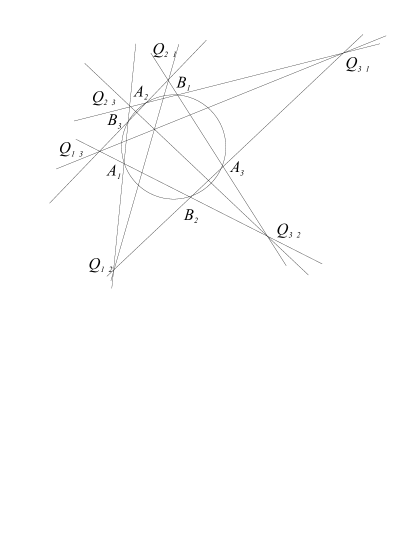
Figure 2: A generalization of the Pascal theorem

Theorem 1.3 (Generalized Pappus theorem).

Let the conditions of the Pappus theorem be fulfilled. Then the lines $Q_{12}Q_{21}$, $Q_{13}Q_{31}$, and $Q_{23}Q_{32}$ meet in a point.

Proof.

Consider the triangles $Q_{12}Q_{23}Q_{31}$ and $Q_{21}Q_{32}Q_{13}$. The intersection points of the opposite sides of these triangles are exactly the points dealt with in the Pascal theorem (for the hexagon $A_{1}B_{3}A_{2}B_{1}A_{3}B_{2}$). Therefore these triangles are perspective from a line and hence from a point. This completes the proof. ∎

Let us give another, well-known way to generalize the Pascal theorem.

Theorem (Another generalization of the Pascal theorem).

Denote $S_{ik}=A_{i}A_{j}\cap B_{j}B_{k}$. Then the three lines $l_{i}=S_{jk}S_{kj}$ meet in a point.

Proof.

Denote $S=A_{3}B_{3}\cap A_{2}B_{2}$. By the Pascal theorem (using a slightly different enumeration of points), the points $S$, $S_{32}$, and $S_{23}$ are collinear. Applying the Pappus theorem to the triples $B_{3}$, $S_{13}$, $B_{2}$ and $A_{2}$, $S_{21}$, $B_{3}$, we infer that the point $U=B_{2}S_{21}\cap A_{3}S_{13}$ belongs to $l$. Applying the Pappus theorem to the triples $B_{2}$, $S_{12}$, $S_{13}$ and $A_{3}$, $S_{31}$, $S_{21}$, we infer that the point $Z=S_{12}S_{21}\cap S_{13}S_{31}$ belongs to $l$. This completes the proof. ∎

1.3 Projective duality

Let us consider the main construction on the projective plane. Notice that projective transformations preserve all the elements of the construction. Moreover, from the projective viewpoint, the choice of the point $S$ and of the lines $\ell_{1}$, $\ell_{2}$, and $\ell_{3}$ does not lead to loss of generality. Indeed, using a suitable projective transformation, we can map this triple of concurrent lines into any other triple of concurrent lines. In particular, the structure of the “additive group of triangles” described in Section  2 does not depend on this choice.

Let us choose a polar transform of the projective plane. Applying it to all the elements of the main configuration, we obtain a theorem dual to Theorem 1.1:

Theorem 1.4.

Let the triangles $A=A_{1}A_{2}A_{3}$ and $B=B_{1}B_{2}B_{3}$ be perspective from a line $s$. For $i=1$, $2$, $3$, let $L_{i}$ denote the intersection points of the corresponding sides: $L_{i}=A_{k}A_{j}\cap B_{k}B_{j}$. Let $C_{k}=A_{i}B_{j}\cap A_{j}B_{i}$. Then the triangle $C=C_{1}C_{2}C_{3}$ is perspective to the triangles $A_{1}A_{2}A_{3}$ and $B_{1}B_{2}B_{3}$ from the line $s$ (see fig. 3).

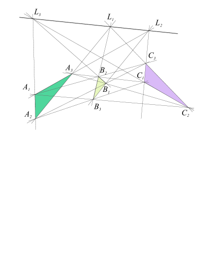
Figure 3: The dual to the main construction

Since a polar transform is involutory, Theorem 1.4 follows from Theorem 1.1.

Definition 1.3 (Central and axis models).

The construction used in Theorem 1.1 (fig. 1) will be referred to as the central model. The construction used in Theorem 1.4 (fig. 3) will be referred to as the axis model.

In the central model we fix the point $S$ and the three lines $\ell_{1}$, $\ell_{2}$, $\ell_{3}$ that pass through this point. In the axis model we fix the line $s$ and the three points $L_{1}$, $L_{2}$, $L_{3}$ that belong to this line. For brevity of notations, we denote by $A$ the triangle $A_{1}A_{2}A_{3}$ (where $A_{i}\in\ell_{i}$ for the central model; $A_{i}A_{j}$ contains the point $L_{k}$ for the axis model).

2 Additive group of triangles

Let us remind how the addition of points on an elliptic curve is defined. First, one introduces certain “geometric” construction. Given two points $A$ and $B$ on an elliptic curve, this construction allows us to construct one more point of the curve, $C$. Namely, $C$ is the third point where the line $AB$ intersects the elliptic curve. Denote this as $C=A\cdot B$. Now the addition operation is defined as follows. We fix an arbitrary point $E$ on the curve and put $A+B=E\cdot(A\cdot B)$. The point $E$ plays the role of a neutral element (the “zero”).

However, this method requires a discussion of certain technical details. And it turns out that it is natural to consider the curve not on a plane but on the complex projective plane. The definition of the point $C$ requires further conventions if $A=B$ or if the line $AB$ is tangent to the curve. Finally, one often chooses as $E$ a point at infinity. This leads to a somewhat “mysterious” definition of the sum: having constructed the point $A\cdot B$, one symmetrically reflects it with respect to the axis $x$. The top of the theory is a construction of elliptic functions that are homomorphisms between the additive group of points of an elliptic curve and the complex torus.

In this section we will define an addition operation on the set of perspective triangles. The configuration theorem given in the previous subsection (Theorem 1.4) allows us to construct a triangle by two given triangles. This however requires some technical comments, for instance, in the case of coinciding triangles. In order to define the addition we need only to repeat the operation with a fixed triangle. However, to introduce such an operation, it requires a certain completion of the set of triangles. It is convenient to choose an “infinitely remote triangle” as the fixed element. Then the barycentric coordinates will play the role of an elliptic function.

2.1 Sum of perspective triangles

Definition 2.1.

Let $A$ and $B$ be two triangles perspective from a point $S$ or a line $s$. By the generalized Desargues theorem, these triangles define the third triangle, $C$, which we call the pre-sum of the triangles $A$ and $B$. We denote this as $C=A\boxplus B$.

Let us describe some obvious properties of this operation.

Lemma 2.1.

The operation “pre-sum” possesses the following properties:

1) $A\boxplus B=B\boxplus A$.

2) If $A\boxplus B=C$, then $A\boxplus C=B$ and $B\boxplus C=A$.

Remark 2.1.

The set of triangles is not closed with respect to the operation “pre-sum”. For example, the reader can easily see from the fig. 1 that all the three vertices of the triangle $C$ can coincide with the point $S$ for a certain choice of the triangles $A$ and $B$.

Definition 2.2.

Let $F$ be an arbitrary fixed triangle. The sum of triangles $A$ and $B$ is defined as $A+B=F\boxplus(A\boxplus B)$ whenever this formula makes sense.

Remark 2.2.

A set equipped with an operation that has properties as in Lemma 2.1 is called a quasi-group. Let us stress that the axioms of a quasi-group do not imply associativity of the operation $A+B=F\boxplus(A\boxplus B)$. For instance, applying the Pappus theorem, we can construct from two triples of collinear points $A$ and $B$ the third triple, $C=A\boxplus B$. It is easy to verify that such an operation satisfies Lemma 2.1. But then a “sum” arising by an analogy with Definition 2.2 is not associative.

Further we will deal with the axis model. Let the perspective axis, $s$, be at infinity (this can be always achieved with the help of an appropriate projective transformation). For technical reasons, it is convenient to choose $F$ to be an infinitely remote triangle (this notion will be clarified later). Thus, in the rest of the paper we will use the following definition of the sum.

Definition 2.3.

Let $A$ and $B$ be triangles perspective from a line $s$, and let $C=A\boxplus B$. Let $C_{0}$ denote the mass center of the triangle $C$. Let $D$ be a triangle that is centrally symmetric to the triangle $C$ with respect to the point $C_{0}$. We call $D$ the sum of the triangles $A$ and $B$ and write this as $D=A+B$.

We will prove below that this operation is commutative and associative (which justifies calling it a sum). We will show that the symmetry with respect to the mass center is actually a computation of the pre-sum of a given triangle with a certain “infinitely remote triangle” (see Example 3.3). The latter will play the role of the neutral element (the “zero”) for the addition operation. Let us remark that the operation defined in Definition 2.2 is also commutative and associative and gives rise to the same Abelian group. The proof of this is completely analogous to that in the case of the sum defined in Definition 2.3.

2.2 Barycentric coordinates and the space of triangles

Applying an appropriate projective transformation, we can always achieve that the line $s$ in the axis model is at infinity. In this case the corresponding sides of the triangles $A$, $B$, and $C=A\boxplus B$ are parallel (see fig. 4). Below we understand by triangles only triangles which have the same directions of sides.

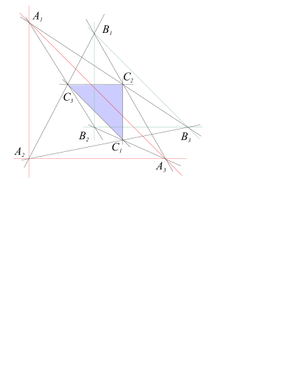
Figure 4: The dual construction with an axis at infinity

Choose any triangle $E=E_{1}E_{2}E_{3}$. Below we understand by coordinates of a point on the affine plane the barycentric coordinates of this point with respect to the triangle $E$ (see [5]). With the help of these coordinates we will introduce coordinates on the set of triangles.

Definition 2.4 (Barycentric coordinates on the set of triangles).

Every triangle $D$ is uniquely determined by the coordinates $(d_{1},d_{2},d_{3})$ (where $d_{1}+d_{2}+d_{3}=1$) of its mass center and by the coefficient $d$ of the only homothecy which transforms $D$ into $E$ (the parallel translation is by definition a homothecy with $d=1$). Consequently, this triangle is uniquely determined by a triple of parameters, $(\delta_{1},\delta_{2},\delta_{3})$, such that

$$\delta_{1}:\delta_{2}:\delta_{3}=d_{1}:d_{2}:d_{3}\,,\qquad\delta_{1}+\delta_{2}+\delta_{3}=d\,.$$

The parameters $(\delta_{1},\delta_{2},\delta_{3})$ are called the barycentric coordinates of the triangle $D$.

The connection between the coordinates ($d_{1}$, $d_{2}$, $d_{3}$; $d$) and the barycentric coordinates $(\delta_{1},\delta_{2},\delta_{3})$ is given by

$$\delta_{i}=d\cdot d_{i}\qquad\ d=\delta_{1}+\delta_{2}+\delta_{3};\quad d_{i}=\frac{\delta_{i}}{d}=\frac{\delta_{i}}{\sum\delta_{i}}\quad(i=1,2,3).$$

Example 2.1.

Let us find the coordinates of the vertices of a triangle $D=D_{1}D_{2}D_{3}$ with the mass center $D_{0}$ in terms of its barycentric coordinates $\delta_{1}$, $\delta_{2}$, $\delta_{3}$. For this purpose we notice that the vector $\overrightarrow{D_{0}D_{3}}$ is homothetic to the vector $\overrightarrow{E_{0}E_{3}}$ with a coefficient $\frac{1}{d}$:

$$D_{3}=D_{0}+\frac{1}{d}\,(E_{3}-E_{0})=\frac{1}{d}\,(\delta_{1},\delta_{2},\delta_{3})+\frac{1}{d}\,\Bigr{(}\!-\frac{1}{3},-\frac{1}{3},\frac{2}{3}\Bigl{)}=\Bigl{(}\frac{\delta_{1}-1/3}{d},\frac{\delta_{2}-1/3}{d},\frac{\delta_{3}+2/3}{d}\Bigr{)}.$$

Coordinates of the other vertices are computed analogously.

Let us remark that there exists no (geometric) triangle if the sum of the coordinates vanishes.

Definition 2.5.

Let us extend the set of geometric triangles by adding formal elements whose barycentric coordinates are given by parameters $(\delta_{1},\delta_{2},\delta_{3})$ with $\delta_{1}+\delta_{2}+\delta_{3}=0$. We call the resulting space the space of triangles; it is formally isomorphic to $\mathbb{R}^{3}$.

Triangles which have small sum of their coordinates are of a “big size”. It is therefore natural to expect that the formal elements admit an interpretation as “infinitely remote” triangles (see Section 3.1).

2.3 The main theorem

Theorem 2.1.

The operation “$+$” defined in Definition 2.3 coincides, in the barycentric coordinates, with the addition operation in $\mathbb{R}^{3}$.

Proof.

Let $A$ and $B$ be two triangles with coordinates $(\alpha_{1},\alpha_{2},\alpha_{3})$, $\sum\alpha_{i}=a\neq 0$, and $(\beta_{1},\beta_{2},\beta_{3})$, $\sum b_{i}=b\neq 0$, respectively. Let their pre-sum $C=A\boxplus B$ be also a triangle, i.e., $\sum\gamma_{i}=c\neq 0$ for coordinates $(\gamma_{1},\gamma_{2},\gamma_{3})$ of $C$. Let us find the coordinates of the triangle $C$. The triangles $A_{1}C_{3}A_{2}$ and $B_{2}C_{3}B_{1}$ (see fig. 4) are homothetic; the homothecy coefficient is $A_{2}A_{1}/B_{2}B_{1}=\frac{1/a}{1/b}$. Hence $a\cdot A_{1}C_{3}=b\cdot C_{3}B_{2}$. This implies that the point $C_{3}$ is the mass center of the points $(a,A_{1})$ and $(b,B_{2})$. That is,

$$C_{3}=\frac{1}{a+b}\,(a\cdot A_{1}+b\cdot B_{2})=\frac{1}{a+b}\,\bigl{(}(\alpha_{1}+2/3,\alpha_{2}-1/3,\alpha_{3}-1/3)+(\beta_{1}-1/3,\beta_{2}+2/3,\beta_{3}-1/3)\bigr{)}=\\ =\Bigl{(}\frac{-(\alpha_{1}+\beta_{1})-1/3}{-(a+b)},\frac{-(\alpha_{2}+\beta_{2})-1/3}{-(a+b)},\frac{-(\alpha_{3}+\beta_{3})+2/3}{-(a+b)}\Bigr{)}\,.$$ (1)

Coordinates of the points $C_{1}$ and $C_{2}$ are found in the same way. Notice that

$$C_{2}-C_{1}=\frac{1}{-(a+b)}\,(-1,1,0)=\frac{1}{-(a+b)}\,(E_{2}-E_{1})\,.$$

Therefore, the sum of coordinates of the triangle $C$ (which is the homothecy coefficient of $C\rightarrow E$) equals to $-(a+b)$. Multiplying this quantity by the coordinates of the mass center $C_{0}$ of the triangle $C$, we will obtain the coordinates of $C$. The coordinates of $C_{0}$ are given by

$$\frac{C_{1}+C_{2}+C_{3}}{3}=\left(\frac{-(\alpha_{1}+\beta_{1})}{-(a+b)},\frac{-(\alpha_{2}+\beta_{2})}{-(a+b)},\frac{-(\alpha_{3}+\beta_{3})}{-(a+b)}\right)\,.$$

Therefore, the coordinates of the triangle $C$ are

$$(-(\alpha_{1}+\beta_{1}),-(\alpha_{2}+\beta_{2}),-(\alpha_{3}+\beta_{3}))\,.$$ (2)

It is clear that the central symmetry transformation with respect to the mass center reverses the coordinates of a triangle. Thus, coordinates of the sum $A+B$ equal to

$$(\alpha_{1}+\beta_{1},\alpha_{2}+\beta_{2},\alpha_{3}+\beta_{3})\,.$$ (3)

∎

Corollary.

The operation “$+$” defined in Definition 2.3 extends to a commutative and associative operation on the space of triangles. The resulting “additive group of triangles” is isomorphic to the additive group $\mathbb{R}^{3}$.

3 Technical details

3.1 Geometric interpretation of formal triangles

As we show below, almost all formal triangles admit a geometric interpretation.

Definition 3.1 (Barycentric coordinates on the line at infinity).

Let $X$ be a point with barycentric coordinates $(x_{1},x_{2},x_{3})$, $\sum x_{i}=1$. Then $\overrightarrow{OX}=\sum x_{i}\overrightarrow{OE_{i}}$ for any point $O$. Similarly, for a triple of numbers $(y_{1},y_{2},y_{3})$ with vanishing sum, we can consider vector $\sum y_{i}\overrightarrow{OE_{i}}$. Apparently, this vector does not depend on $O$. Therefore, the triple $(y_{1},y_{2},y_{3})$ determines a direction (in fact, a vector; the direction is obtained after a factorization over the scalar multiplier). We call the homogeneous triple $(y_{1},y_{2},y_{3})$ the barycentric coordinates of this direction (= coordinates of a point on the line at infinity).

Definition 3.2.

A pseudo-triangle with coordinates $(p_{1},p_{2},p_{3})$, $\sum p_{i}=0$, is an ordered triple of directions with the following coordinates

$$(p_{1}+\tfrac{2}{3},p_{2}-\tfrac{1}{3},p_{3}-\tfrac{1}{3}),\quad(p_{1}-\tfrac{1}{3},p_{2}+\tfrac{2}{3},p_{3}-\tfrac{1}{3}),\quad(p_{1}-\tfrac{1}{3},p_{2}-\tfrac{1}{3},p_{3}+\tfrac{2}{3})\,.$$

The points of the line at infinity corresponding to these directions (or the directions themselves) are called the vertices of the pseudo-triangle. A formal element of the space of triangles with coordinates $(p_{1},p_{2},p_{3})$, $\sum p_{i}=0$, is regarded as a pseudo-triangle $(p_{1},p_{2},p_{3})$.

Example 3.1.

Let $A$ and $C$ be triangles that are centrally symmetric to each other with respect to a point which is not the middle of any of the sides of these triangles. Let us find their pre-sum. Constructing the main configuration, we observe that the lines $A_{i}C_{j}$ and $A_{j}C_{i}$ are parallel for all pairs $i$, $j$ (see fig. 5). Thus, the “triangle” $A\boxplus C$ is a triple of points at infinity, i.e., it is a pseudo-triangle.

Example 3.2.

What is a pseudo-triangle which has coordinates $(0,0,0)$ ? Its vertices are the directions $(\frac{2}{3},-\frac{1}{3},-\frac{1}{3})$, $(-\frac{1}{3},\frac{2}{3},-\frac{1}{3})$, $(-\frac{1}{3},-\frac{1}{3},\frac{2}{3})$. Choosing the mass center of the triangle $E$ as the point $O$ in Definition 3.1, we see that these directions are the directions of the medians of the triangle $E$ (or of any other triangle).

On the projective plane, the main construction without any additional conventions allows us to find the sum of a triangle and a pseudo-triangle.

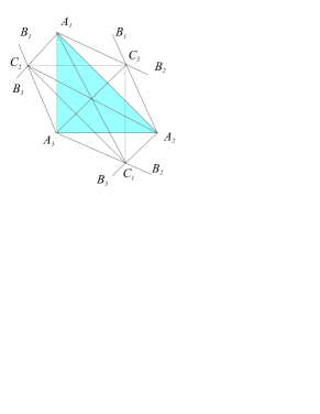
Figure 5: Addition of a triangle with the zero triangle

Example 3.3.

Let us find the pre-sum of a triangle $A$ and the pseudo-triangle $B$ with coordinates $(0,0,0)$. Vertices of the pseudo-triangle $B(0,0,0)$ are the directions of the medians of the triangle $A$ (see Example 3.2). Constructing the main configuration, we obtain that the pre-sum in question is simply the reflection of the triangle $A$ with respect to its mass center (see fig. 5).

Let us remark that, although the barycentric coordinates are defined up to multiplication by a constant, pseudo-triangles with distinct coordinates correspond to different triples of directions.

The definition of a pseudo-triangle does not make sense only for the three sets of parameters: $(-\frac{2}{3},\frac{1}{3},\frac{1}{3})$, $(\frac{1}{3},-\frac{2}{3},\frac{1}{3})$, and $(\frac{1}{3},\frac{1}{3},-\frac{2}{3})$ since, by virtue of Definition 3.1, points of the line at infinity can not have three vanishing coordinates.

Definition 3.3.

The three formal elements of the space of triangles, which have the coordinates $(-\frac{2}{3},\frac{1}{3},\frac{1}{3})$, $(\frac{1}{3},-\frac{2}{3},\frac{1}{3})$, or $(\frac{1}{3},\frac{1}{3},-\frac{2}{3})$, are called the completely-pseudo-triangles.

Thus, the formal elements in Definition 2.5 are either pseudo-triangles or completely-pseudo-triangles. This classification is exhausting.

3.2 Corrections to the main construction

As before, we deal with the axis model. It is easy to see that certain ambiguities in the main construction for triangles $A$ and $B$ appear in the three following cases:

1) if two sides of the triangles $A$ and $B$ belong to the same line (e.g., if the points $A_{1}$, $A_{2}$, $B_{1}$, $B_{2}$ are collinear, then the lines $A_{1}B_{2}$ and $A_{2}B_{1}$ coincide and the vertex $C_{3}$ is not defined);

2) if $A=B$ (which is a stronger degeneration of the previous case; here none of the vertices of the triangle $C$ is defined);

3) if the triangles $A$ and $B$ are centrally symmetric to each other with respect to the middle of their (common) side (say, if $A_{1}A_{2}=B_{2}B_{1}$, then the lines $A_{1}B_{2}$ and $A_{2}B_{1}$ are not defined).

In the first two cases the pre-sum is a triangle; in the third case it is a completely-pseudo-triangle. Below we explain how to modify the main construction so that the pre-sum for these degenerate cases can be found geometrically.

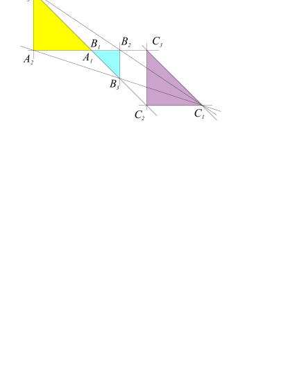
Figure 6: The simplest degenerate case of pre-summation

3.2.1 The case of two coinciding sides

Assume that $A_{1}=B_{1}$ but $A_{2}\neq B_{2}$ and that the triangles $A$ and $B$ are not centrally symmetric to each other (see fig. 6). Then $C_{1}$ is determined by the main construction. About $C_{2}$ and $C_{3}$ we know only that $C_{2}\in A_{1}B_{3}=B_{1}A_{3}$ and $C_{3}\in A_{1}B_{2}=A_{2}B_{1}$. This information allows us to construct $C_{2}$ and $C_{3}$ geometrically (say, $C_{2}=A_{1}B_{3}\cap C_{1}S_{3}$, where $S_{3}$ is the infinitely remote point of the line $A_{1}A_{2}$). The case of $A_{2}=B_{1}$ and the case when the points $A_{1}$, $B_{1}$, $A_{2}$, $B_{2}$ lie on a line can be treated analogously. In all these cases the coordinates of the pre-sum are given by the formula (2). This is clear from taking a limit.

3.2.2 Geometric definition of $A\boxplus A$

Let us require that the property $A\boxplus(A\boxplus A)=A$ hold. In the central model, this implies that the vertices of the triangle $A$ belong to the sides of the triangle $A\boxplus A$. Let us construct $A\boxplus A$. Denote $X_{i}=A_{j}A_{k}\cap SA_{i}$ (see fig. 7). Let $Y_{j}$ be the harmonic complement of the point $S$ to the pair $\{A_{j},X_{j}\}$. Then three quadruples of the form $\Gamma_{j}=\{S,Y_{j}\}\{A_{j},X_{j}\}$ are harmonic. Projecting the quadruple $\Gamma_{j}$ from the point $A_{i}$ onto the line $SA_{k}$, we obtain a harmonic quadruple $\{S,Y_{k}^{\prime}\}\{X_{k},A_{k}\}$, where $Y_{k}^{\prime}=A_{i}Y_{j}\cap SA_{k}$. This implies that the points $Y_{k}$ and $Y_{k}^{\prime}$ coincide since they both are harmonic complements of the point $S$ to the pair $\{A_{k},X_{k}\}$. Consequently, the points $A_{i}$, $Y_{j}$, $Y_{k}$ are collinear. Therefore, $Y_{1}Y_{2}Y_{3}$ is the desired triangle $A\boxplus A$.

Let us remark that $X_{1}X_{2}X_{3}=A/2$ in the sense that $X_{1}X_{2}X_{3}\boxplus X_{1}X_{2}X_{3}=A$.

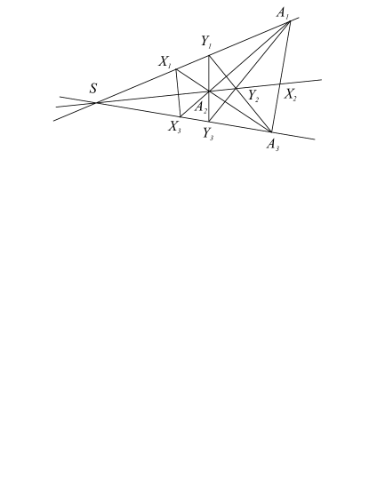
Figure 7: Adding a triangle to itself

For the axis model, the condition “the vertices of $A$ lie on the sides of $A\boxplus A$” is replaced with the condition “the vertices of $A\boxplus A$ lie on the sides of $A$”. This means that $A\boxplus A$ is the triangle whose vertices are the middles of the sides of $A$. It is easy to see that this synthetic definition is consistent with Definition 2.4 and the formula (2).

3.2.3 Sum of triangles that are symmetric with respect to the middle of a side

In this case we can suggest only a formal rule.

Assume that $A_{1}=B_{2}$ and $A_{2}=B_{1}$. Then the main construction allows us to construct two (infinitely remote) vertices. The third vertex, $A_{1}B_{2}\cap A_{2}B_{1}$, is not defined. In the case under consideration we have $\alpha_{1}+\alpha_{2}+\alpha_{3}=-(\beta_{1}+\beta_{2}+\beta_{3})$. Analogously to Example 2.1, we verify that coordinates of the triangles satisfy the following relations

$$\alpha_{1}=-\beta_{1}-\frac{1}{3},\quad\alpha_{2}=-\beta_{2}-\frac{1}{3},\quad\alpha_{3}=-\beta_{3}+\frac{2}{3}\,.$$

In this case we can define the resulting pre-sum as the completely-pseudo-triangle with coordinates $(-\frac{1}{3},-\frac{1}{3},\frac{2}{3})$.

Conversely, adding the completely-pseudo-triangle $(-\frac{1}{3},-\frac{1}{3},\frac{2}{3})$ with a triangle $A$, we obtain a triangle that is symmetric to $A$ with respect to the side $A_{1}A_{2}$.

These definitions are consistent with the properties in Lemma 2.1 and perfectly agree with the formula (2).

3.3 Pre-sum of two pseudo-triangles

It is not difficult to verify that the pre-sum on the projective plane of two centrally symmetric triangles with coordinates $(\alpha_{1},\alpha_{2},\alpha_{3})$ and $(\beta_{1},\beta_{2},\beta_{3})$ (see Example 3.1) is a pseudo-triangle with coordinates $p_{i}=-(\alpha_{i}+\beta_{i})$. That is the formula (2) is satisfied. One can similarly compute coordinates of the pre-sum of a triangle and a pseudo-triangle.

In order to give a geometric description of addition of pseudo-triangles, we consider the following parameterization of the space of pseudo- (including completely-pseudo-) triangles. We regard pseudo- and completely-pseudo-triangles as pre-sums of a fixed triangle (e.g., the triangle $E$) with those that are symmetric to it. We regard these symmetric triangles as parameters of pseudo-triangles.

It can be shown (for instance, employing the barycentric coordinates) that for every pseudo-triangle there exists a unique parameterizing triangle. Pre-summation of pseudo-triangles is described by the following lemma:

Lemma 3.1.

If triangles $B$ and $C$ are symmetric to the triangle $E$ and pseudo-triangles $X$ and $Y$ are defined as the pre-sums $E\boxplus B$ and $E\boxplus C$, then $X\boxplus Y=E\boxplus D$, where $D_{i}$ are the middle points of the intervals $B_{i}C_{i}$.

The proof is left for an interested reader.

Acknowledgment: The authors are grateful to A. Bytsko for help with translation of the manuscript.

Department of mathematics and mechanics
St.Petersburg State University
Bibliotechnaya pl. 2
198904 St.Petersburg, Russia

e-mail: kostik@kk1437.spb.edu, fedor@fp5607.spb.edu

References

- [1] Coxeter, H.S.M. and Greitzer, S.L.: Geometry revisited (Random House, NY, 1967).
- [2] Hilbert, D. and Cohn-Vossen, S.: Geometry and the imagination (Chelsea Publishing Co., NY, 1952).
- [3] Prasolov, V. and Solovyev, Y.: Elliptic functions and elliptic integrals, Translations of Mathematical Monographs, v. 170 (AMS, Providence, RI, 1997).
- [4] Efimov, N.V: Higher geometry (English transl.) (Mir Publishers, Moscow,1980).
- [5] Balk, M.B. and Boltyanskij, V.G.: Geometry of masses (in Russian), Bibliotechka “Kvant”, v. 61 (Nauka, Moscow, 1987).