Generalised Thurston-Bennequin invariants for real algebraic surface singularities

Abstract.

A generalised Thurston-Bennequin invariant for a Q-singularity of a real algebraic variety is defined as a linking form on the homologies of the real link of the singularity. The main goal of this paper is to present a method to calculate the linking form in terms of the very good resolution graph of a real normal unibranch singularity of a real algebraic surface. For such singularities, the value of the linking form is the Thurston-Bennequin number of the real link of the singularity. As a special case of unibranch surface singularities, the behaviour of the linking form is investigated on the Brieskorn double points $x^{m}+y^{n}\pm z^{2}=0$.

1. Introduction

The link of a real algebraic surface singularity is a contact 3-manifold with the canonical contact structure the set of complex tangencies. Furthermore, the real link in this contact manifold is a Legendrian link. The linking form is defined as a rational valued form on the first homology of the real link whenever the rational linking number is well-defined in the link of the singularity, i.e. when the link is a $\mathbb{Q}$-homology sphere (see Section 2.2 or [9] for the definition of the linking form). For such a link, the linking form, when evaluated on a pair of classes of knots of the real link, gives the rational linking number of the knots with contact framing. In the case when the real link is connected, i.e. the singularity is unibranch, the outcome of the linking form is by definition the Thurston-Bennequin number.

Therefore, one can consider the linking form as a generalised Thurston-Bennequin invariant. It is generalised in the sense that (i) it is defined for a link in a contact manifold, (ii) the knots of the link are not necessarily integrally null-homologous but they bound rationally, (iii) it is rational valued.

A method to compute this linking form has already been presented for surface singularities $f(x,y)\pm z^{2}=0$ ($f(x,y)$ reduced) using real deformations of the singularity [10].

The main result of this paper is Theorem 15, Section 5, which presents a method to calculate the generalised Thurston-Bennequin number of the connected real link of a normal real algebraic surface Q-singularity using a very good resolution graph of the singularity with the condition that the singularity is numerically Gorenstein. In particular, Theorem 15 is valid for all the unibranch hypersurface singularities in $\mathbb{C}^{3}$. Furthermore, we give an example which exhibits how the method works algorithmically for singularities with more than one real branch.

In the proof of Theorem 15, we make use of the fact that the generalised Thurston-Bennequin number of the connected real link of a surface singularity gives by definition the self-intersection of the oriented real part of the surface in the complex surface relative to the link of the singularity. This is not valid anymore if the real part is non-oriented. Theorem 15 determines how much the generalised Thurston-Bennequin number differs from the self-intersection of the real part. This difference is a non-integer rational number in general.

In the second part of the article, as a special case of hypersurface singularities, for which Theorem 15 is valid, we deduce some properties for the Thurston-Bennequin numbers of the Brieskorn double points $x^{m}+y^{n}\pm z^{2}=0$ with $m$, $n$ relatively prime. We first express the conditions under which the Thurston-Bennequin numbers become integer (see Corollary 18 and Corollary 20, Section 6). Then we investigate the behaviour of the Thurston-Bennequin numbers with changing $m$ and $n$ (see Theorems 21, 22 and 24, Section 6). These theorems show that one can calculate the Thurston-Bennequin numbers for large $m$ and $n$ in terms of the Thurston-Bennequin numbers corresponding to sufficiently small $m$ and $n$

The main approach in the proofs is to use Theorem 15. In fact, Corollary 18 is a direct consequence of Theorem 15. We prove Corollary 20 and Theorem 21 by observing the change in the very good resolution graph of the singularity when $m$ is held fixed and $n$ is varied (see Section 3) and using the results of Section 4.

The proofs of Theorems 22 and 24, Section 6, do not involve resolution graphs. Rather, we construct new real algebraic surfaces as branched double coverings of appropriate weighted homogeneous surfaces; these new algebraic surfaces contain at the same time both singularities involved in each theorem.

Notation: In this article, the manifold $\overline{X}$ is usually the quotient of the manifold $X$ by complex conjugation except in the case $\overline{\mathbb{C}P^{2}}$ which is $\mathbb{C}P^{2}$ with reverse orientation.

Acknowledgments. I would like to thank Sergey Finashin (METU, Ankara) for having introduced me the problem, for his invaluable guidance and his inspiration and to Yıldıray Ozan (METU, Ankara) for many stimulating discussions. In addition, I would like to thank CMAT, Ecole Polytechnique, Palaiseau where I completed this work as a postdoc.

2. Preliminary notions and definitions

2.1. The real branches of a real surface Q-singularity and the linking form

Let $\mathbb{C}X$ be the complex point set of a real algebraic surface with complex conjugation ${\rm conj}:\mathbb{C}X\rightarrow\mathbb{C}X$; let $\mathbb{R}X$ denote the set of the real points of $\mathbb{C}X$ and $\overline{X}$ denote the quotient $\mathbb{C}X/{\rm conj}$. Let $x$ be an isolated singularity of $\mathbb{C}X$ and $\mathbb{C}U$ be a small compact cone-like neighbourhood of $x$ [16].

It is known that the boundary $\mathbb{C}M=\partial\,\mathbb{C}U$ is a 3-manifold with a canonical contact structure determined by the distribution of complex lines that exist uniquely in the tangent space over each point of $\mathbb{C}M$ [22]. Furthermore, since the real link $\mathbb{R}M$ is tangent to the unique complex line at each point, $\mathbb{R}M$ is a Legendrian link in $\mathbb{C}M$. Although $\mathbb{C}M$ is not a complex manifold, we use the notation with prefix $\mathbb{C}$ to emphasize that $\mathbb{C}M$ is fixed under ${\rm conj}$ of $\mathbb{C}X$. With the same idea in mind, $\mathbb{R}M$ denotes the subset of $\mathbb{C}M$ fixed pointwise by ${\rm conj}$. Finally $\overline{M}$ will denote $\partial\overline{U}$.

A singular point $x\in\mathbb{C}X$ is called a topologically rational singularity (or a Q-singularity) if its link $\mathbb{C}M$ is a $\mathbb{Q}$-homology sphere. Point $x$ is called a $\overline{Q}$-singularity if $\overline{M}$ is a $\mathbb{Q}$-homology sphere. Let $x\in\mathbb{C}X$ be a Q-singularity and let $\sigma$ denote the number of connected components of the real link $\mathbb{R}M$. Each connected component of $\mathbb{R}M$ is called a real branch of $\mathbb{C}X$ at $x$. If $\sigma=1$, i.e. if $\mathbb{R}M$ is a knot, then we will say that $x$ is a real unibranch singularity. For example, the Brieskorn singularity $\{x^{m}+y^{n}+z^{d}=0\}$, $\gcd(m,n,d)=1$ is an isolated Q-singularity which is a real unibranch singularity.

Let $\gamma_{1},\ldots,\gamma_{\sigma}$ be the connected components of $\mathbb{R}M$ and $\xi_{i}$ be a Thurston-Bennequin framing of $\gamma_{i}$ in $\mathbb{C}M$, i.e. a choice of trivialisation of a tubular neighbourhood of $\gamma_{i}$ in $\mathbb{C}M$. Let us denote by $\gamma_{i}^{\xi_{i}}$ the knot obtained by a small shift of $\gamma_{i}$ in the direction of $\xi_{i}$. Consider the bilinear form

$${\rm tb}_{x}:H_{1}(\mathbb{R}M;\mathbb{Q})\times H_{1}(\mathbb{R}M;\mathbb{Q})\rightarrow\mathbb{Q}$$

defined on the generators by:

$${\rm tb}_{x}([\gamma_{i}],[\gamma_{j}])={\rm lk}(\gamma_{i},\gamma_{j}^{\xi_{j}})\mbox{ in }\mathbb{C}M$$

and extended linearly over $H_{1}(\mathbb{R}M;\mathbb{Q})$ (see [9] or [10]). Here lk is the rational linking number in $\mathbb{C}M$. Note that if $i=j$, then ${\rm tb}_{x}([\gamma_{i}],[\gamma_{i}])={\rm tb}(\gamma_{i})$, the rational Thurston-Bennequin number of the Legendrian knot [3]. The form ${\rm tb}_{x}$ is called the linking form.

It is essential to note the following: Let $\sigma_{i}$ denote the component of closure of $\mathbb{R}U-\{x\}$ containing $\gamma_{i}$; the real surface $\sigma_{i}$ is a cone over $\gamma_{i}$ topologically. Consider a tangent vector field $\nu_{i}$ on $\sigma_{i}$ directed outward along $\gamma_{i}$. Then $\sqrt{-1}\cdot\nu_{i}$ coincides with $\xi_{i}$, the Thurston-Bennequin framing, proving that in case $\sigma_{i}$ and $\sigma_{j}$ are oriented, the form ${\rm tb}_{x}$ evaluated on $[\gamma_{i}]$ and $[\gamma_{j}]$ is nothing but the rational intersection of $\sigma_{i}$ and $\sigma_{j}$ in $\mathbb{C}U$ relative to the boundary, i.e. :

(1) $${\rm tb}_{x}([\gamma_{i}],[\gamma_{j}])=\langle\sigma_{i},\sigma_{j}\rangle_{(\mathbb{C}U,\mathbb{C}M)}.$$

Similarly as above, for a $\overline{Q}$-singularity, one can define a bilinear form $\overline{{\rm tb}}_{x}$ on $H_{1}(\mathbb{R}M;\mathbb{Q})$ by letting

$$\overline{{\rm tb}}_{x}([\gamma_{i}],[\gamma_{j}])={\rm lk}(q(\gamma_{i}),q(\gamma_{j}^{\xi_{j}}))\mbox{ in }\overline{M}=q(\mathbb{C}M)$$

where $q:\mathbb{C}X\rightarrow\overline{X}$ is the quotient map. For a $\overline{Q}$-singularity, ${\rm tb}_{x}$ and $\overline{{\rm tb}}_{x}$ satisfy [10]:

(2) $$\overline{{\rm tb}}_{x}=2\,{\rm tb}_{x}.$$

The linking form ${\rm tb}_{x}$ corresponding to a singularity with $\sigma$ real branches is represented by a $\sigma\times\sigma$ matrix. We are going to denote by $[{\rm tb}_{x}]$ the $\sigma\times\sigma$ matrix in the basis $\gamma_{1},\ldots,\gamma_{\sigma}$. We will not mention $\gamma_{i}$s whenever there is no confusion and we will also allow permuted indexing. The matrix $[{\rm tb}_{x}]$ of a real unibranch singularity $x$ is a $1\times 1$ matrix and in that case, ${\rm tb}_{x}$ will be called the Thurston-Bennequin number of the real unibranch singularity $x$ as well.

An algorithmic method was introduced in [10], Theorem B, to compute the Thurston-Bennequin numbers of the real unibranch singularities $f(x,y)\pm z^{2}=0$ where $f(x,y)$ is a real polynomial with an isolated real singularity. This method makes use of the diagrams of Gusein-Zade [13] and A’Campo [1] which are obtained by small real generic deformations of the singularity $f(x,y)=0$ in $\mathbb{C}^{2}$.

A more general approach for computation of the Thurston-Bennequin number associated to a normal unibranch Q-singularity was partly announced in [10] using a resolution of the singularity. Below, Theorem 15, Section 5, offers a method to compute the Thurston-Bennequin number of a real normal unibranch Q-singularity using a very good resolution graph of the singularity. In the case the real part of the ambient real algebraic surface is oriented, Theorem 15 gives Equation 1.

2.2. Resolution graphs

Let $\mathbb{C}X$ be a normal complex surface and $\rho:\mathbb{C}\widetilde{X}\rightarrow\mathbb{C}X$ be a resolution of $\mathbb{C}X$. The preimage $E=\rho^{-1}({\rm sing}(\mathbb{C}X))\subset\mathbb{C}\widetilde{X}$ is called the exceptional set and each irreducible curve in the exceptional set is called an exceptional curve of the resolution $\rho$. Let the number of exceptional curves in $E$ be $s$; then the exceptional curves of $E$ will be denoted by $E_{1},\ldots,E_{s}$.

The resolution $\rho$ is said to be good if the exceptional curves are smoothly embedded and any two intersecting exceptional curves intersect at normal crossings. A very good resolution is a good resolution with any pair of exceptional curves having at most one common point. A good and a very good resolution always exist for any analytic surface (cf. [15] or [7]).

The dual graph of a resolution of a surface singularity is constructed by representing each exceptional curve by a vertex and connecting two vertices by an edge if the corresponding exceptional curves intersect. It is well known that the dual graph $\Gamma$ of a good resolution of a normal surface singularity is connected. The $s$ vertices $e_{1},\ldots,e_{s}$ of $\Gamma$ correspond to $E_{1},\ldots,E_{s}$ respectively. Each vertex $e_{i}$ ($1\leq i\leq s$) is endowed with a pair of integers: the self intersection $n_{i}$ and the genus $g_{i}$ of $E_{i}$. Two vertices $e_{i}$ and $e_{j}$ are connected by $n_{ij}$ edges where $n_{ij}$ is the number of points in $E_{i}\cap E_{j}$.

From now on, let us assume that $\Gamma$ is the dual graph of a very good resolution $\rho:\mathbb{C}\widetilde{X}\rightarrow\mathbb{C}X$ and also that $\Gamma$ is a tree.

If a vertex $e$ of $\Gamma$ is connected to more than two vertices, then $e$ is called a rupture vertex. A vertex adjacent to one and only one vertex of $\Gamma$ is called a terminal vertex. The star of a subgraph $\sigma$ of $\Gamma$ is a subgraph of $\Gamma$ consisting of $\sigma$ and all the edges connected to any vertex of $\sigma$. The star of $\sigma$ is denoted by ${\rm star}(\sigma)$ (see Figure 1).

a rupture vertex

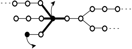
a terminal point

Figure 1. A terminal point, a rupture vertex and its star

Let $e$ be a vertex of $\Gamma$. Let us denote by $\Gamma_{e}$ the subgraph $\Gamma-{\rm star}(e)$ of $\Gamma$. Since $\Gamma$ is a tree, the graph $\Gamma_{e}$ is disconnected if $e$ is not a terminal vertex. Each connected component of $\Gamma_{e}$ is called an arm of $e$. The number of arms of $e$ is equal to the number of edges connected to $e$.

Let $e_{1},\ldots,e_{k}$ be a set of vertices of a graph $\Gamma$. The subgraph spanned by the vertices $e_{1},\ldots,e_{k}$ is the subgraph of $\Gamma$ consisting of the vertices $e_{1},\ldots,e_{k}$ and all the edges of $\Gamma$ connecting any pair of vertices $e_{i}$ and $e_{j}$ with $1\leq i,j\leq k$.

The complex conjugation ${\rm conj}$ of $\mathbb{C}\widetilde{X}$ induced by that of $\mathbb{C}X$ defines a map on the vertices of $\Gamma$ as the following:

$${\rm conj}(e_{i})=\bar{e}_{i}=\left\{\begin{array}[]{ll}e_{i},&\mbox{if $E_{i}$ is real}\\ e_{j},&\mbox{if }{\rm conj}(E_{i})=E_{j}.\end{array}\right.$$

This map is 1-1 and onto since each exceptional curve $E_{i}$ is either real or it does not contain any real point at all. In fact, any normal singularity of a complex surface locally can be thought of as a branched cover of $\mathbb{C}^{2}$ branched along a singular curve [15]. Hence a resolution of the singularity can be constructed (as in Section 3) by taking the branched cover of a resolution of $\mathbb{C}^{2}$ and then by normalizing. Each exceptional curve in the resolution of $\mathbb{C}^{2}$ can be made real so that, in the cover, the preimage of each exceptional curve is real. This said, the claim follows (for this fact see [11] or for real resolutions see [21]).

Now, if an exceptional curve is real, the corresponding vertex will be called real; otherwise it will be called an imaginary vertex. Note that the map conj on the vertices of a resolution graph is a symmetry of the graph.

Let us denote by $\Gamma_{\mathbb{R}}$ and $\Gamma_{\mathbb{C}}$ the subgraphs spanned by the real and respectively imaginary vertices of $\Gamma$. Furthermore, let ${\mathcal{C}}_{e}$ denote the set of imaginary arms in $\Gamma_{e}$, that is, the arms of $e$ on which every vertex is imaginary.

Let $e$ be a rupture vertex of $\Gamma$. We will assign a weight $n^{\sigma}$ to each imaginary arm $\sigma$ in ${\mathcal{C}}_{e}$ and a number $n^{\prime}_{e}$ to vertex $e$. First assume that the arm $\sigma\in{\mathcal{C}}_{e}$ is a bamboo, i.e. contains no rupture vertex. Let there be $k$ vertices $e_{1},\ldots,e_{k}$ on $\sigma$ such that $e_{i}$ is closer than $e_{j}$ to $e$ if $i<j$ $(1\leq i,j\leq k)$. Then the weight of arm $\sigma$ is defined to be the continued fraction:

$$n^{\sigma}={n_{1}-\frac{1}{n_{2}-\frac{1}{\cdots-\frac{1}{n_{k}}}}}.$$

If the imaginary arms of vertex $e$ are all bamboos, then define:

$$n^{\prime}_{e}=n_{e}-\sum_{\sigma\in{\mathcal{C}}_{e}}\frac{1}{n^{\sigma}}.$$

Now, let an imaginary arm $\sigma\in{\mathcal{C}}_{e}$ consist of vertices $e_{1},\ldots,e_{k}$, some of which may be rupture vertices. For each rupture vertex $e_{i}$ on $\sigma$ compute $n^{\prime}_{e_{i}}$ recursively; furthermore, put $n^{\prime}_{i}=n_{i}$ if $e_{i}$ is a vertex on $\sigma$ that is not a rupture vertex. For a short hand notation, we put $n^{\prime}_{i}=n^{\prime}_{e_{i}}$. Then define

$$n^{\sigma}={n^{\prime}_{1}-\frac{1}{n^{\prime}_{2}-\frac{1}{\cdots-\frac{1}{n^{\prime}_{k}}}}}.$$

2.3. Embedded resolution graphs

Let us consider the reduced real algebraic curve $\mathbb{C}A=\{f(x,y)=0\}$ in $\mathbb{C}^{2}$ with a singularity at 0 and with no other singular point. One can resolve $\mathbb{C}A$ by a series of blow-ups of $\mathbb{C}^{2}$. Topologically the blown-up surface is $\mathbb{C}^{2}\#t\overline{\mathbb{C}P^{2}}$ where $t$ is the number of blowing-ups. Let us denote the resolution by $\rho^{\prime}:\mathbb{C}\widetilde{Y}\rightarrow\mathbb{C}^{2}$ where $\mathbb{C}\widetilde{Y}=\mathbb{C}^{2}\#t\overline{\mathbb{C}P^{2}}$. The preimage $(\rho^{\prime})^{-1}(\mathbb{C}A)$ as a divisor is called the total transform of $\mathbb{C}A$. The closure of the preimage $(\rho^{\prime})^{-1}(\mathbb{C}A-\{0\})$ as a divisor is called the proper transform of $\mathbb{C}A$, denoted by $\mathbb{C}\widetilde{A}$. Each component of $\mathbb{C}\widetilde{A}$ is smooth and can be made to transversally intersect the exceptional curves by sufficiently many blow-ups at the points of non-transversal intersection.

Let us furnish the resolution graph corresponding to the resolution $\rho^{\prime}$ with the following further data. Let the number of exceptional curves of $\rho^{\prime}$ be $t$. Each component of the proper transform $\mathbb{C}\widetilde{A}$ which intersects an exceptional curve $E_{i}$ ($1\leq i\leq t$) is specified in the resolution graph by an arrow attached to the vertex $e_{i}$. For instance, if $f(x,y)$ is irreducible, then there exists one arrow on the graph. Furthermore, each vertex $e_{i}$ is assigned a multiplicity $m_{i}\in\mathbb{Z}$; each arrow is assigned a multiplicity 1. Such an ‘extended’ graph is called an embedded resolution graph and is denoted by $\Gamma_{f}$. It is easy to see that $\Gamma_{f}$ is always a tree with arrows.

We extend the definition for a rupture vertex on an embedded resolution graph as follows: A vertex of $\Gamma_{f}$ which is adjacent to more than two vertices or two vertices and an arrow is called a rupture vertex of $\Gamma_{f}$.

The multiplicity $m_{i}$ of an exceptional curve $E_{i}$ is the vanishing order of the map $f\circ\rho^{\prime}:\widetilde{Y}\rightarrow\mathbb{C}$ on $E_{i}$. In other words, in the chart of $\widetilde{Y}$ containing the intersection point of $E_{i}$ and $E_{j}$, the neighbourhood of the intersection can be viewed as $\{(x,y)\in\mathbb{C}^{2}|x^{m_{i}}y^{m_{j}}=0\}$ with an appropriate choice of local coordinates $(x,y)$.

It is well known that the following identity is satisfied on $\Gamma_{f}$ for every $k$, $1\leq k\leq t$ (cf. e.g. [12], p. 251):

(3) $$n_{k}m_{k}+\sum_{\stackrel{{\scriptstyle 1\leq i\leq t}}{{i\neq k,n_{ik}\neq 0}}}m_{i}=0.$$

As a special case, it is going to be useful to understand the algorithmic construction of the embedded resolution graph for $f(x,y)=x^{m}+y^{n}$, $\gcd(m,n)=1$. Assume that $m>n$. One can immediately observe that the blow-up sequence associated to the singularity of $f(x,y)=0$ at 0 is directly related with the Euclidean algorithm for $m$ and $n$:

$$m=q_{l}n+r_{l};$$

$$n=q_{l-1}r_{l}+r_{l-1};$$

$$r_{l}=q_{l-2}r_{l-1}+r_{l-2};$$

$$\cdots$$

$$r_{3}=q_{1}r_{2}+1;$$

$$r_{2}=q_{0}\cdot 1$$

where $r_{l}<n$, $r_{i}\in\mathbb{Z}^{+}$ and $r_{i-1}<r_{i}$ for all $i$ with $1<i<l$. The line containing $q_{i}$ above corresponds to $q_{i}$ consecutive blow-ups so that there are $\sum_{i=0}^{l}q_{i}$ vertices of $\Gamma_{f}$. Let us index the vertices of $\Gamma_{f}$ in the following way: $e_{q_{i},j}$ with $0\leq i\leq l$ and $1\leq j\leq q_{i}$ denotes the vertex created by $j^{\rm th}$ blow-up within the $q_{i}$ consecutive blow-ups. The unique arrow is attached to the vertex $e_{q_{0},q_{0}}$. The graph $\Gamma_{f}$, the vertices $e_{q_{i},j}$ and their multiplicities are shown in Figure 2.

$m_{i}:\;\;n$            $q_{l}n$                 $\cdots$              $q_{l-1}m$         $q_{l}n\!+\!r_{l}=m$

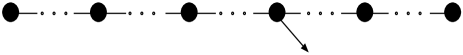
$\underbrace{\mbox{ \hskip 51.21504pt}}_{\displaystyle q_{l}\mbox{ times}}$             $\underbrace{\mbox{ \hskip 51.21504pt}}_{\displaystyle q_{0}\mbox{ times}}$            $\underbrace{\mbox{ \hskip 51.21504pt}}_{\displaystyle q_{l-1}\mbox{ times}}$

Figure 2.

The unique rupture vertex $e_{q_{0},q_{0}}$ of $\Gamma_{f}$ will be denoted by $e_{0}$. The arm of $e_{0}$ with the terminal vertex of multiplicity $n$ (respectively $m$) will be called an ($n$)-arm (respectively ($m$)-arm) of $\Gamma_{f}$.

3. Resolution graphs of Brieskorn double points

Let $f(x,y)=x^{m}+y^{n}$, $\mathbb{C}X$ be the double branched cover of $\mathbb{C}^{2}$ determined by $f(x,y)\pm z^{2}=0$, the branching locus being $\mathbb{C}A=\{f(x,y)=0\}$. Note that the Brieskorn double surface $\mathbb{C}X$ has a normal Q-singularity at 0 (see e.g. [20], Chapter 1).

We are going to consider the commutative diagram:

$$\begin{array}[]{rcl}\mathbb{C}\widetilde{X}&\stackrel{{\scriptstyle\textstyle\rho}}{{\longrightarrow}}&\mathbb{C}X\\ \widetilde{p}\Big{\downarrow}&&\Big{\downarrow}p\\ \mathbb{C}\widehat{A}\subset\mathbb{C}\widetilde{Y}&\stackrel{{\scriptstyle\textstyle\rho^{\prime}}}{{\longrightarrow}}&\mathbb{C}^{2}\supset\mathbb{C}A\end{array}$$

where $p:(x,y,z)\mapsto(x,y)$ is the projection, $\rho:\mathbb{C}\widetilde{X}\rightarrow\mathbb{C}X$ is a very good resolution and $\widetilde{p},\rho^{\prime}$ are defined as follows.

The non-singular surface $\mathbb{C}\widetilde{X}$ can be constructed in two steps. This construction, which is sketched below, can be traced, for example, in [14], Section 0; [12] Section 7.2 or [17]. At the first step, the embedded resolution graph $\Gamma_{f}$ is constructed. Furthermore, if two exceptional curves with odd multiplicities intersect, they are made disjoint by an additional blow-up at the point of intersection. Denote the graph obtained in that way by $\Gamma^{\prime}_{f}$ and the corresponding resolution by $\rho^{\prime}:\mathbb{C}\widetilde{Y}=\mathbb{C}^{2}\#s\overline{\mathbb{C}P}^{2}\rightarrow\mathbb{C}^{2}$ where $s$ is the number of blow-ups employed so far.

Next, let $\mathbb{C}\widehat{A}\subset\mathbb{C}\widetilde{Y}$ be the union of the proper transform $\mathbb{C}\widetilde{A}=(\rho^{\prime})^{-1}(\mathbb{C}A)$ and the exceptional curves in $\mathbb{C}\widetilde{Y}$ with odd multiplicity. The double covering of $\mathbb{C}\widetilde{Y}$ branched along $\mathbb{C}\widehat{A}$ with an appropriate choice of real structure gives $\mathbb{C}\widetilde{X}$. The covering map is denoted by $\widetilde{p}$.

If $E_{i}$ is an exceptional curve in $\mathbb{C}\widetilde{Y}$ with odd multiplicity, then the preimage $\widetilde{p}^{-1}(E_{i})$ is connected and has self intersection $\frac{n_{i}}{2}$. An exceptional curve $E_{i}$ of even multiplicity intersects either with two vertices of odd multiplicity or with no vertices of odd multiplicity. In case of former, $\widetilde{p}^{-1}(E_{i})$ is connected and has self intersection $2n_{i}$. In the latter case, $\widetilde{p}^{-1}(E_{i})$ is constituted of two exceptional curves, each with self-intersection $n_{i}$.

The graph constructed in this way is a good resolution graph and can be changed into a minimal good resolution graph by blowing-down the $(-1)$-curves that do not intersect more than two exceptional curves. We are going to denote by $\Gamma(m,n)$ the resolution graph corresponding to $\rho$.

Let the graph $\Gamma(m,n)$ have $r$ vertices. and let $E^{i}$ (respectively $e^{i}$) ($1\leq i\leq s$) denote the exceptional curves of $\rho$ (respectively the corresponding vertices of $\Gamma(m,n)$). The covering map $\widetilde{p}:\mathbb{C}\widetilde{X}\rightarrow\mathbb{C}\widetilde{Y}$ induces a map $\widetilde{p}:\Gamma(m,n)\rightarrow\Gamma_{f}$, sending $e^{i}$ to $e_{j}$ if $E^{i}$ lies in $\widetilde{\rho}^{-1}(E_{j})$.

The following facts on $\Gamma_{f}$ and $\Gamma(m,n)$ are direct consequences of the algorithm summarised above and at the end of previous section.

Lemma 1.

Let $f(x,y)=x^{m}+y^{n}$ $(\gcd(m,n)=1)$, $e_{0}$ be the rupture vertex of $\Gamma_{f}$ and $\widetilde{p}:\Gamma(m,n)\rightarrow\Gamma_{f}$ be the covering map induced by $\widetilde{p}:\mathbb{C}X=\{x^{m}+y^{n}\pm z^{2}=0\}\rightarrow\mathbb{C}^{2}\#t\overline{\mathbb{C}P}^{2}$. Then:

(i) Multiplicity of $e_{0}=m_{e_{0}}=mn$.

(ii) $\widetilde{p}^{-1}(e_{0})$ is one vertex. Let us denote it by $e^{0}\in\Gamma(m,n)$.

(iii) Let $\sigma$ be an arm of $e_{0}$. Each connected subgraph of $\Gamma(m,n)$ in the preimage $\widetilde{p}^{-1}(\sigma)$ is an arm of $e^{0}$.

(iv) There are $\gcd(m,2)$ arms of $e^{0}$ in the preimage of an ($n$)-arm of $\Gamma_{f}$. Analogously, there are $\gcd(n,2)$ arms of $e^{0}$ in the preimage of an ($m$)-arm.

(v) Number of arms of $e^{0}$ is 3 and each arm of $e^{0}$ is a bamboo.

The fact (iii) above allows the following definition: each arm of $\Gamma(m,n)$ in the preimage of an ($n$)-arm of $\Gamma_{f}$ will be called an ($n$)-arm of $\Gamma(m,n)$. Analogous definition is made for an ($m$)-arm of $\Gamma(m,n)$.

Note that any real algebraic surface defined as a double cover of $\mathbb{C}^{2}$ branched along the reduced curve $\{f(x,y)=0\}$ can be assigned two complex conjugations (see e.g. [5], Section 2.2.4). For the case of Brieskorn double surfaces when $f(x,y)=x^{m}+y^{n}$, let us denote the complex conjugations by ${\rm conj}_{\pm}$ and the corresponding complex surfaces $\{x^{m}+y^{n}\pm z^{2}=0\}$ by $\mathbb{C}X_{\pm}$. First, we give a proof of the following fact pointed out in [10]:

Proposition 2.

Let $\Gamma_{\mathbb{R}}^{\pm}(m,n)$ be the subgraph spanned by the vertices of $\Gamma(m,n)$ fixed under the action of ${\rm conj}_{\pm}$. If $m$ and $n$ are odd, then

$$\Gamma_{\mathbb{R}}^{\pm}(m,n)=\Gamma(m,n).$$

If $m$ is odd and $n$ is even, then

$$\Gamma_{\mathbb{R}}^{-}(m,n)=\Gamma(m,n)$$

and $\Gamma_{\mathbb{R}}^{+}(m,n)$ is the subgraph of $\Gamma(m,n)$ spanned by the rupture vertex and the the ($n$)-arm.

Proof.

If $m$ and $n$ are both odd, then the resolution graph $\Gamma(m,n)$ has no symmetry but the identity. Since complex conjugations correspond to symmetries of the resolution graph, both choices of complex conjugation coincide and all exceptional curves are fixed under conjugation of either choice so that the first assertion follows.

Now let us assume that $m$ is odd and $n$ is even. Let $f(x,y)=x^{m}+y^{n}$ and let $e_{0}$ be the rupture vertex of $\Gamma_{f}$. The multiplicity $m_{0}$ of $E_{0}$ is $mn$ and the self intersection is $-1$. The embedded resolution graph $\Gamma_{f}$ around the vertex $e_{0}$ is shown in Figure 3(a). The two vertices $e_{1}$ and $e_{2}$ adjacent to $e_{0}$ have multiplicities of different parities by Equation 3, Section 2.3. Let us assume that $m_{1}$ is odd and $m_{2}$ is even. In a properly chosen chart of $\mathbb{C}^{2}\#t\overline{\mathbb{C}P}^{2}$ around the point of intersection $E_{0}\cap E_{1}$, the configuration of the exceptional curves $E_{0}$, $E_{1}$, $E_{2}$ and the proper transform $\mathbb{C}\widetilde{A}$ is shown in Figure 3(b). The curve $E_{1}\cup\mathbb{C}\widetilde{A}$ is in the branching locus and is expressed by $x^{mn}(x+1)=0$ in this chart.

$e_{1}$        $e_{0}$        $e_{2}$                            $\mathbb{C}\widetilde{A}$     $E_{1}$        $E_{2}$

$E_{0}$

$-1$

$0$

Figure 3.

Suppose that the double covering $\mathbb{C}X$ of $\mathbb{C}^{2}$ branched along $\mathbb{C}A$ is determined by $\{x^{m}+y^{n}-z^{2}=0\}$. Then above the subset ${\mathcal{S}}=\{(x,y)|-1<x<0\}$ of the chart in Figure 3(b) lie the imaginary points of $\mathbb{C}X$ and above the points outside ${\mathcal{S}}$ on the chart lie the real points of $\mathbb{C}X$. In particular, each connected component of the preimage $\widetilde{p}^{-1}(E_{2})$ is real so that all the exceptional curves on its arm have real connected components on their preimages. Also $\widetilde{p}^{-1}(\mathbb{C}\widetilde{A})$, $\widetilde{p}^{-1}(E_{0})$ and $\widetilde{p}^{-1}(E_{1})$ are real in $\mathbb{C}X$.

Alternatively, suppose that $\mathbb{C}X=\{x^{m}+y^{n}+z^{2}=0\}$. It follows with an analogous argument to the previous paragraph that this time each connected component of the preimage $\widetilde{p}^{-1}(E_{2})$ contains no real point because of the sign change. ∎

Proposition 3.

Let

$$n^{\prime}=\left\{\begin{array}[]{ll}n+2m&m\;\;{\rm odd}\\ n+m&m\;\;{\rm even}.\end{array}\right.$$

For $f(x,y)=x^{m}+y^{n}$ and $f^{\prime}(x,y)=x^{m}+y^{n^{\prime}}$, the resolution graph $\Gamma_{f^{\prime}}$ differs from $\Gamma_{f}$ by a pair of terminal vertices. The outermost vertex has multiplicity $m$ and self intersection $-2$ while the adjacent vertex has multiplicity $2m$ (see Figure 4). Furthermore, the resolution graph $\Gamma(m,n^{\prime})$ differs from $\Gamma(m,n)$ by a terminal vertex on each ($n$)-arm of $\Gamma(m,n^{\prime})$.

Proof.

Let us denote the surfaces $\{f(x,y)+z^{2}=0\}$ and $\{f^{\prime}(x,y)+z^{2}=0\}$ by $X$ and $X^{\prime}$ and the branching curves $\{f(x,y)=0\}$ and $\{f^{\prime}(x,y)=0\}$ by $A$ and $A^{\prime}$ respectively.

$e_{1}\;\;\;\;\;\;\;\;e_{2}$

${\displaystyle{m\atop-2}\;\;\;\;\;{2m\atop n_{2}}}$

Figure 4. $\Gamma_{f^{\prime}}$ has two extra vertices for odd $m$

First suppose that $m$ is odd. Let us blow-up $\mathbb{C}^{2}$ once at 0 to obtain a proper transform $A^{\prime}_{1}\subset\mathbb{C}^{2}\#\overline{\mathbb{C}P}^{2}$ of $A^{\prime}$ and an exceptional curve $E_{1}$ with self intersection $n_{1}=-1$ and multiplicity $m_{1}=m$. Then let us blow-up the $\mathbb{C}^{2}$-chart of $\mathbb{C}^{2}\#\overline{\mathbb{C}P}^{2}$ containing the singular point of $A^{\prime}_{1}$. The exceptional set contains the exceptional curve $E_{1}$ with $n_{1}=-2$ transversally intersecting an exceptional curve $E_{2}$ with $n_{1}=-1$, $m_{2}=2m$. Furthermore the proper transform $A^{\prime}_{2}$ of $A^{\prime}_{1}$ has a singularity at $A^{\prime}_{2}\cap E_{2}$ given locally by $f(x,y)=x^{m}+y^{n}=0$, identical to the curve $A$.

Further blow-ups to resolve the singularity of $A^{\prime}_{2}$ increase the self intersection of $E_{2}$ at least by 1 and produce a proper transform $A^{\prime}_{t}$ of $A^{\prime}$ and the exceptional curves $E_{3},\ldots,E_{t}$. The curves $A^{\prime},E_{3},\ldots,E_{t}$ are transverse to $E_{2}$ and constitute the graph $\Gamma_{f}$ which is a subgraph of $\Gamma_{f^{\prime}}$. Therefore the embedded resolution graph $\Gamma_{f^{\prime}}$ associated to $f^{\prime}$ differs from $\Gamma_{f}$ by the two vertices $e_{1}$ and $e_{2}$ appended to one end of $\Gamma_{f}$.

Now consider the very good resolution $\rho^{\prime}:\widetilde{X^{\prime}}\rightarrow\mathbb{C}^{2}\#t\overline{\mathbb{C}P^{2}}$ associated to $\Gamma_{f^{\prime}}$. The preimages $(\rho^{\prime})^{-1}(E_{1})$ and $(\rho^{\prime})^{-1}(E_{2})$ are rational curves with self intersections $-1$ and $-2n_{2}\leq-4$ respectively. Blowing $(\rho^{\prime})^{-1}(E_{1})$ down, we end up with a vertex on $\Gamma(m,n^{\prime})$ with self intersection at most $-3$ (before further possible blow-downs of $-1$ curves). This vertex is appended to the ($n$)-arm of $\Gamma(m,n)$.

For the case of even $m$, the proof is analogous except that in the beginning one needs to blow-up only once to obtain a new vertex in $\Gamma(m,n^{\prime})$ representing an exceptional curve of multiplicity $m$ and self intersection $-k$. Also note that, different from the odd case, there are two ($n$)-arms on $\Gamma_{f}$ and two ($n^{\prime}$)-arms on $\Gamma_{f^{\prime}}$. ∎

Corollary 4.

$\Gamma(m,n+4m/(m,2))$ differs from $\Gamma(m,n)$ by two extra vertices at the end of each of its ($n$)-arms.

Proposition 5.

The self intersection of the terminal vertex of each ($n$)-arm of the graph $\Gamma(m,n+4m/(m,2))$ is $-2$.

Proof.

Assume first that $m$ is odd. Let $n^{\prime}=n+4m$ and $f^{\prime}(x,y)=x^{m}+y^{n^{\prime}}$. One has the terminal part of an $(n^{\prime})$-arm of $\Gamma_{f^{\prime}}$ as shown in Figure 5(a). To see this one needs to apply four consequent blow-ups as described in the proof of Proposition 3. Then it is straightforward to verify that the terminal part of an ($n^{\prime}$)-arm of $\Gamma(m,n^{\prime})$ is as in Figure 5(b). Blowing down the $(-1)$-curves, the proof follows.

$\!e_{1}^{\prime}\;\;\;\;\;\;\;\;\,e_{1}\;\;\;\;\;\;\;\;\,e_{2}^{\prime}\;\;\;\;\;\;\;\;e_{2}$                    $e_{1}^{\prime}\;\;\;\;\;\;\;\,e_{1}\;\;\;\;\;\;\;\,e_{2}^{\prime}\;\;\;\;\;\;\;\,e_{2}$

${\displaystyle{m\atop-2}\;\;\;\;{2m\atop-2}\;\;\;\;\;\;{3m\atop-2}\;\;\;\;\;\;{4m\atop n_{2}}}$                   $-1\;\;\;\;\;-4\;\;\;\;\;-1\;\;\;\;\;\;\;\;2n_{2}$

(a)                                                              (b)

Figure 5. Resolution graphs (a) $\Gamma_{f^{\prime}}$, (b) $\Gamma(m,n+4m)$ for odd m

The case for even $m$ is similar. ∎

4. The characteristic set of a resolution graph and the first Chern class

Let us consider a very good resolution $\rho:\mathbb{C}\widetilde{U}\rightarrow\mathbb{C}U$ of a compact cone-like neighbourhood $\mathbb{C}U$ of a normal singularity and denote $\mathbb{C}\widetilde{M}=\partial\mathbb{C}\widetilde{U}$. As in [8], let $c$ be the unique class in $H^{2}(\mathbb{C}\widetilde{U},\mathbb{C}\widetilde{M};\mathbb{Q})\equiv H^{2}(\mathbb{C}\widetilde{U},\mathbb{C}\widetilde{M})\otimes\mathbb{Q}$ such that $j^{*}(c)=c_{1}(\mathbb{C}\widetilde{U})\in H^{2}(\mathbb{C}\widetilde{U};\mathbb{Z})$ where $j:\mathbb{C}\widetilde{U}\rightarrow(\mathbb{C}\widetilde{U},\mathbb{C}\widetilde{M})$ is the inclusion map. The canonical class $K\in H_{2}(\mathbb{C}\widetilde{U};\mathbb{Q})$ is defined to be the Lefschetz dual $LD(-c)$ and can be expressed as $\sum_{1\leq i\leq s}a_{i}E_{i}$ where $a_{i}\in\mathbb{Q}$ and $s$ is the number of exceptional curves of the resolution.

If the singularity above is numerically Gorenstein, i.e. $K$ is integral, then $K$ is integral dual to the second Stiefel-Whitney class $w=w_{2}(\mathbb{C}\widetilde{U},\mathbb{C}\widetilde{M};\mathbb{Z})$. Therefore, we can write $w=\sum_{1\leq i\leq s}\hat{a}_{i}E_{i}$ where $\hat{a}_{i}=(a_{i}\!\mod\!2)$ and $E_{i}$ is identified with its dual in $H^{2}(\mathbb{C}\widetilde{U},\mathbb{C}\widetilde{M};\mathbb{Z})$. Note that $w$ satisfies the Wu formula:

(4) $$w\cdot E_{i}\equiv E_{i}\cdot E_{i}\mbox{ (mod 2) for all }i,1\leq i\leq s$$

and furthermore for $1\leq i,j\leq s$, the matrix of the intersection form $Q_{\mathbb{C}\widetilde{U}}$ on $\mathbb{C}\widetilde{U}$ has the entries

$$E_{i}\cdot E_{j}=\left\{\begin{array}[]{ll}n_{ij},&i\neq j\\ n_{i},&i=j\end{array}\right.$$

in the basis $E_{1},\ldots,E_{s}$.

For a normal, numerically Gorenstein Q-singularity, let $\Gamma$ be a very good resolution graph with $s$ vertices and $w$ be expressed as a sum as above. The characteristic set ${\mathcal{W}}$ of $\Gamma$ is defined as the following set of vertices of $\Gamma$:

$${\mathcal{W}}=\{e_{i}\in\Gamma|\hat{a}_{i}=1\}.$$

It is algorithmic to determine the characteristic set of a very good resolution graph. Nevertheless, the relation between $c_{1}(\mathbb{C}\widetilde{U})$ and ${\mathcal{W}}$ may lead to some general properties.

Now let $p:\mathbb{C}X\rightarrow\mathbb{C}^{2}$ be a double covering branched along an irreducible singular curve $\mathbb{C}A=\{f(x,y)=0\}$ that has an isolated singularity at 0. Note that the singularity of $\mathbb{C}X$ is normal and numerically Gorenstein (see e.g. [8]).

As in Section 3, consider the commutative diagram:

$$\begin{array}[]{rcl}\mathbb{C}\widetilde{U}&\stackrel{{\scriptstyle\textstyle\rho}}{{\longrightarrow}}&\mathbb{C}U\\ \widetilde{p}\Big{\downarrow}&&\Big{\downarrow}p\\ \mathbb{C}\widetilde{V}&\stackrel{{\scriptstyle\textstyle\rho^{\prime}}}{{\longrightarrow}}&B^{4}\subset\mathbb{C}^{2}\end{array}$$

where $B^{4}$ is a sufficiently small ball around 0 so that $\mathbb{C}U$ is cone-like. Let $\widetilde{A}$ denote the proper transform of $\mathbb{C}A\cap B^{4}$ under $\rho^{\prime}$ and $\widehat{A}\subset\mathbb{C}\widetilde{V}$ the branching locus of the double covering $\widetilde{p}$; $E^{i}\subset\mathbb{C}\widetilde{U}$ ($1\leq i\leq s$) denote the exceptional curves of the very good resolution $\rho$; $E_{i}\subset\mathbb{C}\widetilde{V}$ ($1\leq i\leq t$) denote the exceptional curves of the resolution $\rho^{\prime}$. Denote the multiplicity of $E_{i}$ by $m_{i}$. We can express

$$c_{1}(\mathbb{C}\widetilde{U})=\sum_{i=1}^{s}a_{i}E^{i},\;\;\;\;\;c_{1}(\mathbb{C}\widetilde{V})=\sum_{i=1}^{s}b_{i}E_{i}.$$

Above and what follows below, $E^{i}\in H_{2}(\mathbb{C}\widetilde{U})$ is always identified with the image $j_{U}^{*}(LD(E_{i}))$ of its Lefschetz dual $LD(E_{i})\in H^{2}(\mathbb{C}\widetilde{U},\partial\mathbb{C}\widetilde{U})$ under the homomorphism $j_{U}^{*}$ induced by the inclusion $j_{U}:\mathbb{C}\widetilde{U}\rightarrow(\mathbb{C}\widetilde{U},\partial\mathbb{C}\widetilde{U})$ and $E_{i}$ is identified with the image $j_{V}^{*}(LD(E_{i}))$ under the inclusion $j_{V}:\mathbb{C}\widetilde{V}\rightarrow(\mathbb{C}\widetilde{V},\partial\mathbb{C}\widetilde{V})$.

Proposition 6.

Assume that $E_{j}=\widetilde{p}(E^{i})$ for some $i$ and $j$ with $1\leq i\leq s$ and $1\leq j\leq t$. If the multiplicity $m_{j}$ of $E_{j}$ is odd then the coefficient $a_{i}$ in $c_{1}(\mathbb{C}\widetilde{U})$ is even.

Proof.

First note that $c_{1}(\mathbb{C}\widetilde{U})=(\widetilde{p})^{*}(c_{1}(\mathbb{C}\widetilde{V})-\frac{1}{2}[\hat{A}])$ (see e.g. [2]). The class $c_{1}(\mathbb{C}\widetilde{V})-\frac{1}{2}[\hat{A}]$ can be expressed as a sum $\sum_{i=1}^{t}d_{i}E_{i}$ in $H^{2}(\mathbb{C}\widetilde{V})$ with $d_{i}\in\mathbb{Z}$. Then,

$$c_{1}(\mathbb{C}\widetilde{U})=(\widetilde{p})^{*}(\sum_{i=1}^{t}d_{i}E_{i})={\displaystyle\sum_{1\leq i\leq t\atop m_{i}{\rm odd}}}2d_{i}(\widetilde{p})^{*}(E_{i})+{\displaystyle\sum_{1\leq i\leq t\atop m_{i}{\rm even}}}d_{i}(\widetilde{p})^{*}(E_{i})$$

which shows that all of the exceptional curves with odd multiplicities have even coefficients in $c_{1}(\mathbb{C}\widetilde{U})$. ∎

Proposition 7.

Assume that $E_{j}=\widetilde{p}(E^{i})$ for some $i$ and $j$ with $1\leq i\leq s$ and $1\leq j\leq t$. Also let $(\widetilde{p})^{*}(\frac{1}{2}[\widehat{A}])=\sum_{k=1}^{s}d_{k}E^{k}$, $d_{k}\in\mathbb{Z}$. Then $d_{i}$ is odd if and only if the multiplicity $m_{j}\equiv 2\mod\,4$.

Proof.

First let us note:

Lemma 8.

${\displaystyle[\widetilde{A}]=-\sum_{l=1}^{t}m_{l}E_{l}.}$

Proof.

The proper transform $\widetilde{A}$ intersects just one exceptional curve, say $E_{r}$. To prove the claim, it is enough to check that

$$Q_{\mathbb{C}\widetilde{V}}\bigg{(}(-\sum_{l=1}^{t}m_{l}E_{l}),E_{r}\bigg{)}=\left\{\begin{array}[]{ll}1,&r=l\\ 0,&r\neq l.\end{array}\right.$$

It is then straightforward to see that this identity is in fact a reformulation of Equation 3, Section 2.3. ∎

Since

$$[\widehat{A}]=[\widetilde{A}]+\sum_{m_{i}{\rm odd}}E_{i},$$

it follows from the lemma that

$$\begin{array}[]{ll}[\widehat{A}]&=-{\displaystyle\sum_{i=1}^{t}}m_{i}E_{i}+{\displaystyle\sum_{1\leq i\leq t\atop m_{i}{\rm odd}}}E_{i}\\ &=-{\displaystyle\sum_{1\leq i\leq t\atop m_{i}{\rm even}}}m_{i}E_{i}+{\displaystyle\sum_{1\leq i\leq t\atop m_{i}{\rm odd}}}(-m_{i}+1)E_{i}.\end{array}$$

Considering the behaviour of the transfer map from $H^{2}(\mathbb{C}\widetilde{U};\mathbb{Z})$ to $H^{2}(\mathbb{C}\widetilde{V};\mathbb{Z})$ one can deduce that

$$(\widetilde{p})^{*}\Big{(}\frac{1}{2}[\widehat{A}]\Big{)}=\sum_{1\leq k\leq t\atop m_{k}{\rm even}}\frac{m_{k}}{2}(\widetilde{p})^{*}\Big{(}E_{k}\Big{)}+\sum_{1\leq k\leq t\atop m_{k}{\rm odd}}(-m_{k}+1)(\widetilde{p})^{*}\Big{(}E_{k}\Big{)}.$$

A coefficient on the right hand side corresponding to $E_{j}$ is odd if and only if $m_{j}\equiv 2\mod\,4$. ∎

The last two propositions now prove

Proposition 9.

Let $E_{j}=\widetilde{p}(E^{i})$ for some $i$ and $j$ with $1\leq i\leq s$ and $1\leq j\leq t$. Then $a_{i}$ is odd if and only if one of the following two conditions holds: (i) $m_{j}\equiv 2\mod\,4$ and $b_{j}$ even; (ii) $4|m_{j}$ and $b_{j}$ odd.

Proposition 10.

Corresponding to the resolution $\rho^{\prime}:\mathbb{C}\widetilde{V}\rightarrow B^{4}$, consider the blow-up sequence:

$$\begin{array}[]{ccccccccccc}\mathbb{C}\widetilde{V}=Y_{t}&\stackrel{{\scriptstyle\textstyle\rho_{t}}}{{\longrightarrow}}&\ldots&\stackrel{{\scriptstyle\textstyle\rho_{k+1}}}{{\longrightarrow}}&Y_{k}&\stackrel{{\scriptstyle\textstyle\rho_{k}}}{{\longrightarrow}}&Y_{k-1}&\stackrel{{\scriptstyle\textstyle\rho_{k-1}}}{{\longrightarrow}}&\ldots&\stackrel{{\scriptstyle\textstyle\rho_{1}}}{{\longrightarrow}}&Y_{0}=B^{4}\subset\mathbb{C}^{2}\\ \cup&&&&\cup&&\cup&&&&\cup\\ \widetilde{A}&\longrightarrow&\ldots&\longrightarrow&A_{k}&\longrightarrow&A_{k-1}&\longrightarrow&\ldots&\longrightarrow&A_{0}=\mathbb{C}A\cap B^{4}\end{array}$$

where $Y_{i}$ ($1\leq i\leq t$) is obtained by blowing up $Y_{i-1}$ at the singular point of $A_{i-1}$, $\rho_{i}$ is the corresponding map and $A_{i}$ is the proper transform of $A_{i-1}$. Let $E_{k}$ denote the exceptional sphere $Cl(\rho_{k}^{-1}(A_{k-1})-A_{k})$ in $Y_{k}$. Assume that $c_{1}(Y_{k})={\displaystyle\sum_{i=1}^{k}}b^{(k)}_{i}E_{i}$, $b^{(k)}_{i}\in\mathbb{Z}$. Then,

$$c_{1}(Y_{k+1})=c_{1}(Y_{k})+\Big{(}\!\!\!-1+\!\!\!\!\sum_{1\leq i\leq k\atop E_{i}\cap E_{k}\neq\emptyset}\!\!b^{(k)}_{i}\Big{)}E_{k+1}.$$

Proof.

It is enough to show that $c_{1}(Y_{k+1})$ as expressed above satisfies the adjunction formula $E_{i}\cdot E_{i}+2=c_{1}(Y_{k+1})(E_{i})$ for all $i$, $1\leq i\leq k+1$. Let $n_{i}^{(k)}$ denote the self intersection of $E_{i}$ in $Y_{k}$. Then the self intersection $n_{i}^{(k+1)}$ of $E_{i}$ in $Y_{k+1}$ is decreased by 1 if $E_{i}\cap A_{k}\neq\emptyset$ in $Y_{k}$ and is unchanged otherwise. Furthermore, $n_{k+1}^{(k+1)}=-1$ and by Equation 3, Section 2.3, $m_{k+1}=1+\!\!\!\!\!\!{\displaystyle\sum_{1\leq i\leq k\atop E_{i}\cap E_{k+1}\neq\emptyset}}\!\!\!\!\!m_{i}$. It is now straightforward to check that $c_{1}(Y_{k+1})$ as given in the form above satisfies the adjunction formula. ∎

Remark 11.

Assume that $c_{1}(Y_{k})=\sum_{i=1}^{k}d_{i}E_{i}$. It follows from the previous proposition that

$$c_{1}(Y_{k-1})=\sum_{i=1}^{k-1}d_{i}E_{i}.$$

Proposition 12.

Let $\mathbb{C}A=\{f(x,y)=x^{m}+y^{n}=0\}\cap B^{4}$ with $\gcd(m,n)=1$. Assume that $E_{i}$ ($1\leq i\leq t$) are as above and that $c_{1}(\mathbb{C}\widetilde{V})=\sum_{i=1}^{t}b_{i}E_{i}$. Then $b_{t}$ is odd if and only if both $m$ and $n$ are odd.

Proof.

Let us adopt the notation of the remark at the end of Section 2.3 so that $t=\sum_{k=0}^{l}q_{k}$. Using Proposition 10, one can algorithmically calculate the coefficients in the expression of $c_{1}(\mathbb{C}\widetilde{V})$. Let $b_{q_{i},j}$ be the coefficient corresponding to vertex $e_{q_{i},j}$. Then, $b_{q_{l},1}=-1,b_{q_{l},2}=-2\ldots b_{q_{l},q_{l}}=-q_{l},b_{q_{l-1},1}=-q_{l}-1,b_{q_{l-1},2}=-2q_{l}-2\ldots b_{q_{l-1},q_{l-1}}=-q_{l-1}q_{l}-q_{l-1}\ldots$ Then it is straightforward to verify by induction on $l$ that:

$$-b_{t}=-b_{q_{0},q_{0}}=q_{l}n+q_{l-1}r_{l}+q_{l-2}r_{l-1}+\ldots+q_{1}r_{2}+q_{0}\cdot 1=m+n-1.$$

Hence the proof follows. ∎

5. Computation of the invariant via resolution graphs

I give the proof of the following fact which was stated in [10].

Proposition 13.

Let $\mathbb{C}E$ be a real rational $(-m)$-curve $(m>0,m\in\mathbb{Q})$ in a real algebraic Q-surface $\mathbb{C}X^{\prime}$. Let $\mathbb{R}E$ be smooth and $\mathbb{R}X^{\prime}$ be nonorientable. Consider the projection $p:\mathbb{C}X^{\prime}\rightarrow X=\mathbb{C}X^{\prime}/\mathbb{C}E$. Then the point $x=p(\mathbb{C}E)\in X$ is a Q-singularity. Furthermore one can define a bilinear form ${\rm tb}_{x}$ on $H_{1}(M)$ (where $M=S_{\epsilon}\cap p(\mathbb{R}X^{\prime})$) by pushing the framings via $p$ as in Section 2.1. The matrix of the form ${\rm tb}_{x}$ in the basis formed by the connected components of $M$ is given by:

$$[{\rm tb}_{x}]=\left\{\begin{array}[]{ccl}\left(\begin{array}[]{rr}-\frac{m}{4}&-\frac{m}{4}\\ -\frac{m}{4}&-\frac{m}{4}\end{array}\right)&,&\mathbb{R}E\mbox{ 2-sided on }\mathbb{R}X^{\prime}\\ (-m)&,&\mathbb{R}E\mbox{ 1-sided on }\mathbb{R}X^{\prime}.\end{array}\right.$$

Proof.

The point $x$ is a Q-singularity because a sufficiently small neighbourhood $\mathbb{C}U^{\prime}$ of $\mathbb{C}E$ in $\mathbb{C}X^{\prime}$ has a boundary which is a $\mathbb{Q}$-homology sphere.

Let $U$ denote $p(\mathbb{C}U^{\prime})$. Let us consider the map $c^{\prime}:\mathbb{C}U^{\prime}\longrightarrow\overline{U}$ of quotient by conjugation.

Assume first that $\mathbb{R}E$ is 2-sided on $\mathbb{R}X^{\prime}$. For $i=1,2$ put $\gamma_{i}=\partial\mathbb{C}U^{\prime}\bigcap\mathbb{R}X^{\prime}$; $\gamma_{1}$ and $\gamma_{2}$ are the two connected components of a small neighbourhood of the cycle $\mathbb{R}E$ in $\mathbb{R}X^{\prime}$. Let $A_{i}$ be the annulus on $\mathbb{R}X^{\prime}$ bounded by $\gamma_{i}$ and $\mathbb{R}E$. Assume that the canonical orientation of the disk $\overline{E}=\mathbb{C}E/{\rm conj}$ agrees with $A_{1}$. Hence, since the surface $\mathbb{R}X^{\prime}$ is nonorientable, the orientation of $\overline{E}$ also agrees with the orientation of $A_{2}$. Now consider the topological disks $\Sigma_{1}=A_{1}\cup_{\mathbb{R}E}\overline{E}$ and $\Sigma_{2}=A_{2}\cup_{\mathbb{R}E}\overline{E}$ in $\overline{U}^{\prime}$. Then it follows from Equation 1, Section 2, that:

$$\overline{tb}_{x}(\gamma_{1},\gamma_{1})=\langle\Sigma_{1},\Sigma_{1}\rangle_{(\overline{U}^{\prime}\!,\partial\overline{U}^{\prime})}=\frac{1}{2}\langle\mathbb{C}E,\mathbb{C}E\rangle_{(\mathbb{C}U^{\prime}\!,\partial\mathbb{C}U^{\prime})}=-\frac{m}{2};$$

$$\overline{tb}_{x}(\gamma_{2},\gamma_{2})=\langle\Sigma_{2},\Sigma_{2}\rangle_{(\overline{U}^{\prime}\!,\partial\overline{U}^{\prime})}=\frac{1}{2}\langle\mathbb{C}E,\mathbb{C}E\rangle_{(\mathbb{C}U^{\prime}\!,\partial\mathbb{C}U^{\prime})}=-\frac{m}{2};$$

$$\overline{tb}_{x}(\gamma_{1},\gamma_{2})=\langle\Sigma_{1},\Sigma_{2}\rangle_{(\overline{U}^{\prime}\!,\partial\overline{U}^{\prime})}=\frac{1}{2}\langle\mathbb{C}E,\mathbb{C}E\rangle_{(\mathbb{C}U^{\prime}\!,\partial\mathbb{C}U^{\prime})}=-\frac{m}{2}.$$

First part of the proof follows from Equation 2, Section 2.1.

Now assume that the cycle $\mathbb{R}E$ is 1-sided on $\mathbb{R}X^{\prime}$. In this case, a sufficiently small neighbourhood of $\mathbb{R}E$ in $\mathbb{R}X^{\prime}$ is a Möbius band, say $A$, thus has connected boundary, say $\gamma$. Observing that $\gamma=2\mathbb{R}E$, define $\Sigma$ to be the relative 2-chain $A\cup_{\mathbb{R}E}2\overline{E}$ in $\overline{U}^{\prime}$. It follows that:

$$\overline{tb}_{x}(\gamma,\gamma)=\langle\Sigma,\Sigma\rangle_{(\overline{U}^{\prime}\!,\partial\overline{U}^{\prime})}=\frac{1}{2}\cdot 4\langle\mathbb{C}E,\mathbb{C}E\rangle_{(\mathbb{C}U^{\prime}\!,\partial\mathbb{C}U^{\prime})}=-2m.$$

∎

Corollary 14.

In the previous proposition, let $\mathbb{R}X^{\prime}$ be orientable. Then

$${\rm tb}_{x}=\left(\begin{array}[]{rr}-\frac{m}{4}&\frac{m}{4}\\ \frac{m}{4}&-\frac{m}{4}\end{array}\right).$$

Proof.

We should only note that in the case of orientable $\mathbb{R}X^{\prime}$, $\mathbb{R}E$ is 2-sided on $\mathbb{R}X^{\prime}$ and the orientation of $\overline{E}$ does not agree with the orientations of $A_{1}$ and $A_{2}$ simultaneously. ∎

Theorem 15.

Let $x\in\mathbb{C}X$ be a normal, numerically Gorenstein, unibranch real Q-singularity; $\mathbb{C}U$ a small compact cone-like real neighbourhood of $x$; $\mathbb{R}M=\mathbb{R}X\cap\partial\mathbb{C}U$; $\Gamma$ be the graph of a very good resolution $\rho:\mathbb{C}\widetilde{U}\rightarrow\mathbb{C}U$ at $x$; $\mathbb{R}\widetilde{U}$ be the preimage $\rho^{-1}(\mathbb{R}U)$; ${\mathcal{W}}_{\mathbb{R}}$ be the characteristic set on $\Gamma_{\mathbb{R}}$ and $N$ be the number of vertices on $\Gamma_{\mathbb{R}}$. Then:

(5) $${\rm tb}(\mathbb{R}M)=N-1+\sum_{\scriptstyle 1\leq i\leq s\atop\scriptstyle e_{i}\in{\mathcal{W}}_{\mathbb{R}}}n^{\prime}_{i}.$$

Proof.

First note that the normality of the singularity $x$ implies that $\Gamma$ is connected. Since $x$ is assumed to be numerically Gorenstein, the canonical class of $\mathbb{C}\widetilde{U}$ is integral so that one can define the characteristic set of the graph. Furthermore since $x$ is a Q-singularity, the graph $\Gamma$ is a tree and each exceptional curve is a sphere (see e.g. [6]).

The surface $\mathbb{R}\widetilde{U}$ is smooth, connected and with boundary $\mathbb{R}M$. $\mathbb{R}\widetilde{U}$ need not to be orientable. It is nonorientable if and only if $n_{i}$ ($1\leq i\leq s$) is odd for at least one real exceptional sphere (see [21], Proposition II.6.9 and Corollary II.6.10). If $n_{i}$ is even for all exceptional spheres, then $\mathbb{R}\widetilde{U}$ is oriented and $c_{1}(\mathbb{C}\widetilde{U})\Big{|}_{\mathbb{R}\widetilde{U}}$ is even, i.e. by definition $\mathcal{W}_{\mathbb{R}}$ is empty, so that the second term on the right hand side of Equation 5 disappears and one obtains Equation 1, Section 2:

$${\rm tb}(\mathbb{R}M)=-\chi(\mathbb{R}\widetilde{U})=N-1.$$

In the general case where $\mathbb{R}\widetilde{U}$ is nonorientable, we construct a real algebraic surface $\mathbb{C}\widehat{U}$ with an oriented real part by getting rid of the terms that appear in $c_{1}(\mathbb{C}\widetilde{U})\Big{|}_{\mathbb{R}\widetilde{U}}$. So, let

$$F=\{E_{i}|e_{i}\in{\mathcal{W}}_{\mathbb{R}}\}\bigcup\{E_{i}|e_{i}\in{\mathcal{C}}_{j}\mbox{ for some }j\,(1\!\leq\!j\!\leq\!s),\mbox{ such that }e_{j}\in{\mathcal{W}}_{\mathbb{R}}\}.$$

We define:

$${\rm pr}:\mathbb{C}\widetilde{U}\rightarrow\mathbb{C}\widehat{U}=\mathbb{C}\widetilde{U}\big{/}F.$$

It is well-known that $c_{1}(\mathbb{C}\widehat{U})|_{\mathbb{R}\widehat{U}}$ is even if and only if $w_{1}(\mathbb{R}\widehat{U})$ is zero. Since each exceptional curve in the canonical class of $\mathbb{C}U$ is contracted in $\mathbb{C}\widehat{U}$, the real part $\mathbb{R}\widehat{U}$ is orientable. However, $\mathbb{R}\widehat{U}$ is not smooth. Let the number of singularities of $\mathbb{C}\widehat{U}$ be $t$ which is exactly the number of vertices in ${\mathcal{W}}_{\mathbb{R}}$. Each singular point is real and is the image ${\rm pr}(E_{i})$ where $E_{i}$ corresponds to the vertex $e_{i}\in{\mathcal{W}}_{\mathbb{R}}$; we denote this singular point by $x_{i}$.

Lemma 16.

Each singular point of $\mathbb{C}\widehat{U}$ is a Q-singularity.

Proof.

Let $x$ be such a singularity. The subgraph of $\Gamma$ spanned by the vertices corresponding to the exceptional spheres in the preimage ${\rm pr}^{-1}(x)$ is a connected, negative definite tree, i.e. a small regular neighbourhood of ${\rm pr}^{-1}(x)$ in $\mathbb{C}\widetilde{U}$ has boundary a $\mathbb{Q}$-homology sphere. ∎

Lemma 17.

Let $x_{i}\in\mathbb{R}\widehat{U}$ be one of above singularities. In the basis of the homology classes of the real branches of $x_{i}$,

$$[{\rm tb}_{x_{i}}]=\left\{\begin{array}[]{ccl}\left(\begin{array}[]{rr}\frac{n^{\prime}_{i}}{4}&\frac{n^{\prime}_{i}}{4}\\ \frac{n^{\prime}_{i}}{4}&\frac{n^{\prime}_{i}}{4}\end{array}\right)&,&\mathbb{R}E\mbox{ 2-sided on }\mathbb{R}X^{\prime}\\ (n^{\prime}_{i})&,&\mathbb{R}E\mbox{ 1-sided on }\mathbb{R}X^{\prime}.\end{array}\right.$$

Proof.

Let $\mathbb{C}\widehat{U}_{x_{i}}\subset\mathbb{C}\widehat{U}$ be a sufficiently small compact cone-like neighbourhood of $x_{i}$ and $\mathbb{C}M_{x_{i}}$ be the boundary $\partial\mathbb{C}\widehat{U}_{x_{i}}$. Let ${\mathcal{E}}$ denote the subspace of $H_{2}({\rm pr}^{-1}(\mathbb{C}\widehat{U}_{x_{i}}))$ generated by the homology classes of exceptional spheres in ${\rm pr}^{-1}(x_{i})$. The complex intersection form in $\mathbb{C}\widehat{U}_{x_{i}}$ is the restriction of the intersection form in ${\rm pr}^{-1}(\mathbb{C}\widehat{U}_{x_{i}})$ to the orthogonal complement ${\mathcal{E}}^{\perp}$ of ${\mathcal{E}}$ in $H_{2}({\rm pr}^{-1}(\mathbb{C}\widehat{U}_{x_{i}}))$, since the restriction of the intersection form in ${\rm pr}^{-1}(\mathbb{C}\widehat{U}_{x_{i}})$ to ${\mathcal{E}}$ is nondegenerate (see [10], Section 5.2). The result of the corresponding orthogonalisation process on the matrix of the intersection form coincides with the continued fractions of the self intersection numbers of the vertices on the contracted arms. The self intersection of $[E_{i}]$ restricted to the subspace $\langle{\mathcal{E}}^{\perp},[E_{i}]\rangle$ is therefore equal to the number $n^{\prime}_{i}$ defined in Section 2.2. Since the singularity $x_{i}$ is obtained by contracting $E_{i}$, the result follows from Proposition 13. ∎

Now, since $\mathbb{R}\widehat{U}$ is oriented, by Equation 1, Section 2, we get:

$$\begin{array}[]{ll}{\rm tb}(\mathbb{R}M)={\rm tb}(\mathbb{R}\widehat{M})&=\langle\mathbb{R}\widehat{U},\mathbb{R}\widehat{U}\rangle_{(\mathbb{C}\widehat{U}\!,\partial\mathbb{C}\widehat{U})}\\ &=-\chi\big{(}\mathbb{R}\widehat{U}-\{t\mbox{ points}\}\big{)}+{\displaystyle\sum_{\scriptstyle 1\leq i\leq s\atop\scriptstyle e_{i}\in{\mathcal{W}}_{\mathbb{R}}}}\langle\Sigma_{i},\Sigma_{i}\rangle_{(\mathbb{C}\widehat{U}_{x_{i}}\!,\partial\mathbb{C}\widehat{U}_{x_{i}})}\end{array}$$

where $\Sigma_{i}$ is the connected piece of the surface $\mathbb{R}\widehat{U}$ bounded by the connected components of the real link $\mathbb{R}\widehat{M}_{x_{i}}$ of ${x_{i}}$ (number of connected components is either one or two).

For any $e_{i}\in{\mathcal{W}}_{\mathbb{R}}$, first let the curve $\mathbb{R}E_{i}$ be 2-sided on the nonorientable surface $\mathbb{R}\widetilde{U}$ and $\gamma_{i1}$, $\gamma_{i2}$ be the two connected components of $\mathbb{R}\widehat{M}_{x_{i}}$. It easy to see that

$$\begin{array}[]{ll}\langle\Sigma_{i},\Sigma_{i}\rangle_{(\mathbb{C}\widehat{U}_{x_{i}}\!,\partial\mathbb{C}\widehat{U}_{x_{i}})}&={\rm tb}_{x_{i}}(\gamma_{i1},\gamma_{i1})+{\rm tb}_{x_{i}}(\gamma_{i2},\gamma_{i2})+2{\rm tb}_{x_{i}}(\gamma_{i1},\gamma_{i2})\\ &=4\cdot\frac{n^{\prime}_{i}}{4}=n^{\prime}_{i}\end{array}$$

where the second equality follows from Lemma 17. Similarly, letting $\mathbb{R}E_{i}$ be 1-sided on $\mathbb{R}\widetilde{U}$, we get ${\displaystyle\langle\Sigma_{i},\Sigma_{i}\rangle_{(\mathbb{C}\widehat{U}_{x_{i}}\!,\partial\mathbb{C}\widehat{U}_{x_{i}})}=n^{\prime}_{i}.}$ Hence,

$$\begin{array}[]{ll}{\rm tb}(\mathbb{R}M)&=-\chi\big{(}\mathbb{R}\widehat{U}-\{t\mbox{ points}\}\big{)}+{\displaystyle\sum_{\scriptstyle 1\leq i\leq s\atop\scriptstyle e_{i}\in{\mathcal{W}}_{\mathbb{R}}}}n^{\prime}_{i}\\ &=-(2-N-1)+{\displaystyle\sum_{\scriptstyle 1\leq i\leq s\atop\scriptstyle e_{i}\in{\mathcal{W}}_{\mathbb{R}}}}n^{\prime}_{i}\\ &=N-1+{\displaystyle\sum_{\scriptstyle 1\leq i\leq s\atop\scriptstyle e_{i}\in{\mathcal{W}}_{\mathbb{R}}}}n^{\prime}_{i}.\end{array}$$

∎

Note that the above calculation is an application of the Integral Formula (see [9]) applied to dimension two.

Example: Consider the singularity on the surface $\mathbb{C}X_{\pm}=\{x^{5}+y^{8}\pm z^{2}=0\}$ with the resolution graph $\Gamma(5,8)$ as in Figure 6. The five vertices belonging to the characteristic set ${\mathcal{W}}$ are marked with a cross in the figure.

The complex conjugation ${\rm conj}_{-}$ on the resolved surface $\mathbb{C}\widetilde{X}_{-}$ fixes all vertices of $\Gamma(5,8)$ (Proposition 2). Therefore ${\mathcal{W}_{\mathbb{R}}}$ is the set of the five vertices marked. Meanwhile, for $\mathbb{C}\widetilde{X}_{+}$, ${\mathcal{W}_{\mathbb{R}}}$ contains only the rupture vertex. In both cases $\mathbb{R}\widetilde{X}_{\pm}$ is nonorientable.

It follows now from Theorem 15 that

$${\rm tb}_{-}=12-1+5\cdot(-2)=1\mbox{ and }{\rm tb}_{+}=2-1+\big{(}-2-2\cdot(-\frac{9}{11})\big{)}=\frac{7}{11}.$$

The values for ${\rm tb}_{\pm}$ can be calculated by the method in [10] as well giving the same results.

$-2$      $-2$       $-2$       $-2$        $-3$

$-3$    $-2$

$-2$      $-2$       $-2$       $-2$        $-3$

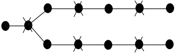
Figure 6. Resolution graph for $x^{5}+y^{8}+z^{2}=0$

5.1. Computation of the linking form for singularities with more than one real branch: an example

Suppose now that the singularity $x\in\mathbb{C}X$ has $\rho$ real branches with $\rho>1$. Then the real part $\mathbb{R}M$ of the link of singularity is disconnected. Hence the linking form ${\rm tb}$ is given by $\rho\times\rho$ matrices. Let us take for example the complex surface $\mathbb{C}X$ defined as the double cover of $\mathbb{C}^{2}$ branched along $\{y(x^{5}+y^{4})=0\}$. The boundary of the surface $\mathbb{R}U$ has two components $\alpha$ and $\beta$. With the methods of [10], one can compute that the $2\times 2$ matrix $[{\rm tb}]$ corresponding to ${\rm tb}$ in the basis $\{[\alpha],[\beta]\}$ is:

$$[{\rm tb}]=\left(\begin{array}[]{rr}{\displaystyle\frac{3}{2}}&{\displaystyle-\frac{5}{2}}\\ {\displaystyle-\frac{5}{2}}&{\displaystyle\frac{3}{2}}\end{array}\right)$$

Alternatively, one can compute this matrix using the arguments in the proof of Theorem 15. The very good resolution graph $\Gamma$ corresponding to the singularity at $0$ is as in Figure 7 where the arrows stand for the two components of the proper transform of the branching locus.

$\hskip 2.84544pt-2\hskip 8.5359pt-2\hskip 11.38092pt-2\hskip 8.5359pt-2\hskip 11.38092pt-2\hskip 8.5359pt-2\hskip 8.5359pt-2\hskip 11.38092pt-2\hskip 8.5359pt\;-2\hskip 11.38092pt-3$

Figure 7. Resolution graph for the singularity $z^{2}=y(x^{5}+y^{4})$

$-2$

There may be assigned two real structures on $\mathbb{C}\widetilde{X}$. Each of the complex conjugations fixes each vertex on the resolution graph. Fix any one of the complex conjugations. Then the surface $\mathbb{R}\widetilde{U}$ is a non-oriented surface with the two boundary components $\alpha$ and $\beta$ (see Figure 8).

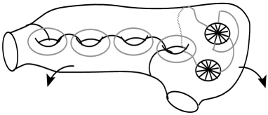
Figure 8. Real part of the surface $\{z^{2}=y(x^{5}+y^{4})\}$ after resolution

$\gamma_{6}$

$\gamma_{7}$

$\gamma_{1}$

$\gamma_{2}\;\;\;\;\;\;\;\;\;\gamma_{3}\;\;\;\;\;\;\;\;\;\gamma_{4}$

$\alpha$                               $\gamma_{5}$

$\Sigma_{1}$                                             $\Sigma_{2}$

$\beta$

Note that the curves $\gamma_{1},\ldots,\gamma_{5}$ separate $\mathbb{R}\widetilde{U}$ into two disjoint surfaces; let us denote by $\Sigma_{1}$ the one which contains $\alpha$ in its boundary and by $\Sigma_{2}$ the other surface. Note that $\Sigma_{1}$ is orientable but $\Sigma_{2}$ is not.

The curves are the real parts of the $-2$-spheres $E_{1},\ldots,E_{5}$. Let ${\mathcal{S}}={e_{1},\ldots,e_{5}}$. Furthermore ${\mathcal{W}}=\{e_{5},e_{6}\}$ is a characteristic set of $\Gamma$.

Similarly as in the proof of Theorem 15, let $F=\{E_{1},\ldots,E_{5},E_{6}\}$ and let ${\rm pr}:\mathbb{C}\widetilde{U}\rightarrow\mathbb{C}\widehat{U}=\mathbb{C}\widetilde{U}\big{/}F$. Let us denote the Q-singularities ${\rm pr}(E_{i})\in\mathbb{C}\widehat{U}$ $(i=1,\ldots 6)$ by $x_{i}$. The surface $\widehat{\Sigma}_{1}={\rm pr}(\Sigma_{1})$ is orientable, has boundary ${\rm pr}(\alpha)$ and contains five Q-singularities $x_{1},\ldots,x_{5}$. The surface $\widehat{\Sigma}_{2}={\rm pr}(\Sigma_{2})$ is orientable, has boundary ${\rm pr}(\beta)$ and contains six Q-singularities $x_{1},\ldots,x_{5},x_{6}$. It follows by the proof of Theorem 15 and Proposition 13 that

$$\begin{array}[]{ll}{\rm tb}(\alpha,\alpha)=\langle\widehat{\Sigma}_{1},\widehat{\Sigma}_{1}\rangle_{\mathbb{C}\widehat{U}\!,\partial\mathbb{C}\widehat{U}}&\displaystyle=-\chi(\widehat{\Sigma}_{1}-\{x_{1},\ldots,x_{5}\})+5\cdot(-\frac{1}{2})=4-\frac{5}{2}=\frac{3}{2};\\ {\rm tb}(\beta,\beta)=\langle\widehat{\Sigma}_{2},\widehat{\Sigma}_{2}\rangle_{\mathbb{C}\widehat{U}\!,\partial\mathbb{C}\widehat{U}}&\displaystyle=-\chi(\widehat{\Sigma}_{2}-\{x_{1},\ldots,x_{6}\})+5\cdot(-\frac{1}{2})+(-2)\\ &\displaystyle=6-\frac{5}{2}-2=\frac{3}{2};\\ {\rm tb}(\alpha,\beta)=\langle\widehat{\Sigma}_{1},\widehat{\Sigma}_{2}\rangle_{\mathbb{C}\widehat{U}\!,\partial\mathbb{C}\widehat{U}}&\displaystyle=5\cdot(\frac{-1}{2})=-\frac{5}{2}={\rm tb}(\beta,\alpha).\end{array}$$

6. On Thurston-Bennequin numbers of Brieskorn double points

The Thurston-Bennequin numbers corresponding to the Brieskorn double points $x^{m}+y^{n}\pm z^{2}=0$ ($\gcd(m,n)=1$) will be denoted by ${\rm tb}_{\pm}(m,n)$.

Corollary 18.

The number ${\rm tb}_{-}(m,n)$ is always an integer.

Proof.

By Proposition 2, Section 3, all vertices of $\Gamma(m,n)$ are fixed under the ${\rm conj}_{-}$, i.e. $\Gamma_{\mathbb{R}}=\Gamma$, so that all the non-integer terms in Equation 5, Section 5, disappear. ∎

The Thurston-Bennequin number ${\rm tb}_{+}(m,n)$ is in general non-integral.

Proposition 19.

Let $m$ be even and $n$ odd. The rupture vertex $e^{0}$ is in ${\mathcal{W}}$ if and only if $4\!\not|m$.

Proof.

The vertex $e_{0}=conj_{\pm}(e^{0})$ in the graph $\Gamma_{f}$ of $\mathbb{C}\widetilde{Y}$ has even multiplicity $mn$. Therefore by Proposition 12 and Proposition 9, Section 4, the proof follows. ∎

Corollary 20.

Assume that $4|m$ and $n$ is odd. Then ${\rm tb}_{+}(m,n)$ is integer.

Proof.

From the proposition above, it follows that there is no (non-integer) contribution of imaginary arms. ∎

The theorem below shows that if the value of $tb_{\pm}(m,n)$ is known for sufficiently small values of $m$ and $n$, the number $tb_{\pm}(m^{\prime},n^{\prime})$ can be computed for greater integers $m^{\prime}$ and $n^{\prime}$.

Theorem 21.

If $m$ is odd then

$${\rm tb}_{\pm}(m,n+4m)={\rm tb}_{\pm}(m,n).$$

If $4|m$ then

$${\rm tb}_{\pm}(m,n+2m)={\rm tb}_{\pm}(m,n).$$

If $m\equiv 2\mod\,4$ then

$${\rm tb}_{-}(m,n+2m)-{\rm tb}_{-}(m,n)=4,$$

$${\rm tb}_{+}(m,n+2m)-{\rm tb}_{+}(m,n)=\frac{4}{n(n+2m)}.$$

Proof.

Assume first that $m$ is odd. By Corollary 4, Section 3, there are two vertices appended to each ($n$)-arm of $\Gamma(m,n)$ to construct $\Gamma(m,n+4m/(m,2))$; let us call them $e_{1}$ and $e_{2}$ with $e_{1}$ being the outer-most vertex. Take an ($n$)-arm of $\Gamma(m,n)$; let us call the two vertices to be appended as $e_{1}$ and $e_{2}$ with $e_{1}$ being the outer-most vertex. By Proposition 5, Section 3, $e_{1}$ has self intersection $-2$.

To prove the theorem, it is enough to show that $e_{1}\in{\mathcal{W}}$ and $e_{2}\not\in{\mathcal{W}}$ since in that case it follows from Theorem 15, Section 5, that

$${\rm tb}_{-}(m,n+4m)={\rm tb}_{-}(m,n)-(-2)+(-2)={\rm tb}_{-}(m,n).$$

Recall that by Proposition 5, the terminal part added to $\Gamma_{f}$ to construct the graph $\Gamma_{f^{\prime}}$ corresponding to $\widetilde{Y}^{\prime}$ is as in Figure 5(a). The exceptional curves $E_{1}^{\prime}$ and $E_{2}^{\prime}$ have odd multiplicities $m$ and $3m$ respectively. Therefore by Proposition 6, Section 4, the vertices of $\Gamma(m,n+4m)$ corresponding to the exceptional curves $\widetilde{p}^{-1}(E^{\prime}_{1})$ and $\widetilde{p}^{-1}(E^{\prime}_{2})$ are not in ${\mathcal{W}}$. It follows that the vertex corresponding to the exceptional curve $\widetilde{p}^{-1}(E_{1})$ must appear in ${\mathcal{W}}$ for Equation 4, Section 4, to be satisfied in $\mathbb{C}\widetilde{U}^{\prime}$. Again in order to satisfy Equation 4, the vertex corresponding to the exceptional curve $E_{2}$ is not included in ${\mathcal{W}}$.

Assume now that $m$ is divisible by 4 and $n$ is odd. By Proposition 2, Corollary 4, Section 3, and Proposition 19, it follows that ${\rm tb}_{+}(m,n+2m)={\rm tb}_{+}(m,n)$. For the relation on the invariant ${\rm tb}_{-}$, we first note that, as in the proof of Proposition 3, Section 3, the terminal part of the resolution graph $\Gamma_{f^{\prime}}$ is as shown in Figure 9. The multiplicity of the sphere $E_{1}$ is $m$ hence by Lemma 7, the preimage $(\widetilde{p})^{*}(E_{1})$ does not contribute mod $2$ to $(\widetilde{p})^{*}(\frac{1}{2}[\widehat{A^{\prime}}])$.

$e_{1}\;\;\;\;\;e_{2}$

${\displaystyle{m\atop-2}\;\;\;\,{2m\atop-k}}$

Figure 9.

The coefficient $b_{1}$ of the cycle $E_{1}$ in $c_{1}(\mathbb{C}\widetilde{V}^{\prime})$ is $-1$ because $E_{1}$ is produced after the first blow-up of $\mathbb{C}^{2}$ (cf. Proposition 10, Section 4). Therefore by Proposition 7, Section 4, the vertex of $\Gamma(m,n+4m)$ corresponding to $\widetilde{p}^{-1}(E_{1})$ is in ${\mathcal{W}}$. As a consequence, $\widetilde{p}^{-1}(E_{2})$ is not in ${\mathcal{W}}$.

(One can also show that $\widetilde{p}^{-1}(E_{2})$ is not in ${\mathcal{W}}$ by the following reasoning: the multiplicity of $E_{2}$ is $2m$. Since $E_{2}$ is produced after the second blow-up of $\mathbb{C}^{2}$, the coefficient $b_{2}$ is $-2$ so that $a_{2}=0\mbox{ mod }2$. Therefore the vertex of $\Gamma(m,n+4m)$ corresponding to $\widetilde{p}^{-1}(E_{2})$ is not in ${\mathcal{W}}$.)

Now assume that $m\equiv 2$ $(\!\!\!\mod\,4)$ and $n$ is odd. The terminal part of the resolution graph $\Gamma_{f^{\prime}}$ is again as in Figure 9. Note that $b_{1}=-1$ and $b_{2}=-2$ so that by Proposition 9, $e_{1},e_{2}\not\in{\mathcal{W}}$. It follows from Theorem 15 that

$$tb_{-}(m,n+2m)-{\rm tb}_{-}(m,n)=-\chi(\mathbb{R}X^{\prime})+\chi(\mathbb{R}X)=2\cdot 2=4.$$

For the last claim in the theorem, we observe by Proposition 19 that $e^{0}\in{\mathcal{W}}_{\mathbb{R}}$. It follows from Corollary 4 that $\Gamma(m,n+2m)$ and $\Gamma(m,n)$ differ in the pair of $(n+2m)$-arms of the former and pair of ($n$)-arms of the latter. Let $\sigma^{\prime}$ be an $(n+2m)$-arm of $\Gamma(m,n+2m)$ and $\sigma$ be an ($n$)-arm of $\Gamma(m,n)$. By Theorem 15

$$tb_{+}(m,n+2m)-{\rm tb}_{+}(m,n)=2(\frac{1}{n^{\sigma^{\prime}}}-\frac{1}{n^{\sigma}}).$$

By [18] Theorem 3.6.1, it follows that

$$\frac{1}{n^{\sigma^{\prime}}}-\frac{1}{n^{\sigma}}=-\frac{1}{m(n+2m)}+\frac{1}{mn}=\frac{2}{n(n+2m)}$$

and the proof follows. ∎

Theorem 22.

Let $m$ be odd and $k,t\in\mathbb{Z}^{+}$, $4km>t$. Then

$${\rm tb}_{\pm}(m,4km-t)+{\rm tb}_{\pm}(m,t)=-2.$$

Proof.

Consider the weighted homogeneous surface $\mathbb{C}P(4k,1,1)$ with a unique singularity at $[1:0:0]$ (cf. [6] Appendix B for a brief introduction to weighted projective spaces) and the curve $\mathbb{C}A=\{x^{m}+u^{4km-t}v^{t}=0\}$ in $\mathbb{C}P(4k,1,1)$. $\mathbb{C}A$ has a pair of singularities at $[0:0:1]$ and $[0:1:0]$. Let $\mathbb{C}\widetilde{P}(4k,1,1)$ obtained by blowing-up $\mathbb{C}P(4k,1,1)$ at $[1:0:0]$. Denote the resolution by $\rho$.

The plan of the proof is as the following. First we construct a branched double covering $p:\mathbb{C}X\rightarrow\mathbb{C}P(4k,1,1)$ whose branching locus contains the curve $\mathbb{C}A$. The surface $\mathbb{C}X$ has the real Brieskorn double points corresponding to $(m,t,2)$ and $(m,4km-t,2)$. Then we show that $\mathbb{R}X$ is orientable and $\overline{X}=\mathbb{C}X/{\rm conj}$ is a $\mathbb{Q}$-homology sphere so that $\big{\langle}\mathbb{R}X,\mathbb{R}X\big{\rangle}_{\overline{X}}=0$. Using this identity, we obtain a relation between ${\rm tb}_{\pm}(m,4km-t)$ and ${\rm tb}_{\pm}(m,t)$.

The smooth surface $\mathbb{C}\widetilde{P}(4k,1,1)$ is biholomorphic to the Hirzebruch surface $\mathbb{F}_{4k}$ and the section $S_{\infty}\subset\mathbb{C}\widetilde{P}(4k,1,1)$ has self intersection $-4k$ (see e.g. [2]). Let $S_{0}$ be the zero section and $F$ be a fiber of ruling in $\mathbb{C}\widetilde{P}(4k,1,1)$. One can show that $[\rho^{-1}(\mathbb{C}A)]\!=\!m[S_{0}]$ and $\big{(}[\rho^{-1}(\mathbb{C}A)]+[S_{\infty}]\big{)}\!=\!(m+1)[S_{0}]-4k[F]$. Hence, $[\rho^{-1}(\mathbb{C}A)]$ is odd and $\big{(}[\rho^{-1}(\mathbb{C}A)]+[S_{\infty}]\big{)}$ is even. Therefore there exist a double covering $\widetilde{p}:\mathbb{C}\widetilde{X}\rightarrow\mathbb{C}\widetilde{P}$ branched along $\rho^{-1}(\mathbb{C}A)\cup S_{\infty}$. The covering $\widetilde{p}$ is associated either with the complex conjugation ${\rm conj}_{-}$ or with $conj_{+}$. Let us assume that $\widetilde{p}$ is associated with ${\rm conj}_{-}$ first.

Consider the commutative diagram:

$$\begin{array}[]{rcccl}\mathbb{C}\widetilde{X}&\stackrel{{\scriptstyle\textstyle\widetilde{\rho}}}{{\longrightarrow}}&\mathbb{C}X&\stackrel{{\scriptstyle\textstyle c^{\prime}}}{{\longrightarrow}}&\mathbb{C}X/{\rm conj}=\overline{X}\\ \widetilde{p}\Big{\downarrow}&&\Big{\downarrow}p&&\Big{\downarrow}\overline{p}\\ \mathbb{F}_{4k}=\mathbb{C}\widetilde{P}(4k,1,1)&\stackrel{{\scriptstyle\textstyle\rho}}{{\longrightarrow}}&\mathbb{C}P(4k,1,1)&\stackrel{{\scriptstyle\textstyle c}}{{\longrightarrow}}&\mathbb{C}P(4k,1,1)/{\rm conj}=\overline{P}\end{array}$$

where $p:\mathbb{C}X\rightarrow\mathbb{C}P(4k,1,1)$ is the double covering with branching locus $\mathbb{C}A\cup\rho(S_{\infty})=\mathbb{C}A\cup\{[1:0:0]\}\subset\mathbb{C}P(4k,1,1)$ and $c$, $c^{\prime}$ are maps of quotient by conjugation. Note that $\mathbb{C}X=\mathbb{C}\widetilde{X}/E$ where $E=\widetilde{p}^{-1}(S_{\infty})$ with $E^{2}=-2$ and $\mathbb{C}X$ has isolated singularities at $p^{-1}([1:0:0])$, $p^{-1}([0:1:0])$ and $p^{-1}([0:0:1])$, the last two being Brieskorn double points corresponding to $(m,t,2)$ and $(m,4km-t,2)$ respectively.

It is easy to check that $c_{1}(\mathbb{C}\widetilde{X})$ is even. Therefore the surface $\mathbb{R}\widetilde{X}$ is orientable. In particular, $\mathbb{R}\widetilde{X}$ is a torus and $\mathbb{R}X$ is a pinched torus. To see this, let $\Delta$ be the subset of $\mathbb{R}\widetilde{P}(4k,1,1)$ such that $\Delta=\widetilde{p}(\mathbb{R}\widetilde{X})$. Then $\Delta$ is the closure of one of the connected components of $\mathbb{R}\widetilde{P}(4k,1,1)-\big{(}\rho^{-1}(\mathbb{R}A)\cup S_{\infty}\big{)}$. Therefore $\Delta$ is an annulus (see Figure 10). Note that the choice of $\Delta$ is determined by the choice of the complex conjugation ${\rm conj}_{\pm}$.

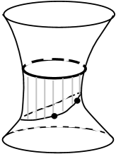
Figure 10. $\mathbb{R}\widetilde{A}\cup\mathbb{R}S_{\infty}$ bounds an annulus on $\mathbb{R}\widetilde{P}(4,1,1)$

$\mathbb{R}S_{\infty}$

$\Delta$

$\rho^{-1}(\mathbb{R}A)$

$\mathbb{R}X$ has three singular points: $P_{1}=p^{-1}([0:1:0])$, $P_{2}=p^{-1}([0:0:1])$ and $P_{3}=p^{-1}([1:0:0])$. The point $P_{3}$ is obtained by contracting $E$ in $\mathbb{C}\widetilde{X}$. It follows from Corollary 14, Section 5, that

(6) $$[{\rm tb}_{P_{3}}]=\left[\!\!\begin{array}[]{rr}-\frac{k}{2}&\frac{k}{2}\\ \frac{k}{2}&-\frac{k}{2}\end{array}\right].$$

Finally we observe that $\overline{P}$ and $\overline{X}$ are $\mathbb{Q}$-homology 4-spheres. For the former, we note the well-known fact that $\mathbb{C}P(k,1,1)$ is a $\mathbb{Q}$-homology manifold with cohomology $H^{*}(\mathbb{C}P(k,1,1);\mathbb{Q})=H^{*}(\mathbb{C}P^{2};\mathbb{Z})\otimes\mathbb{Q}$. Then it follows from [4], Section III.5, that $\overline{P}(k,1,1)$ is a $\mathbb{Q}$-homology sphere.

In order to prove that $\overline{X}$ is a $\mathbb{Q}$-homology sphere, it is enough to show that $\overline{p}:\overline{X}\rightarrow\overline{P}$ is branched along a 2-sphere. In fact, the branching locus is the Arnold surface $\mathcal{A}=\overline{A}\cup_{\partial}c\big{(}\mathbb{R}P(4k,1,1)-\mbox{int}(p(\mathbb{R}X))\big{)}\subset\overline{P}(k,1,1)$ where $\overline{A}=c(\mathbb{C}A)$. Since $\mathbb{C}{A}$ is a sphere, it follows immediately that $\mathcal{A}$ is a sphere.

Therefore there is no rational 2-homology in $\overline{X}$. In particular, the pinched torus $c^{\prime}(\mathbb{R}X)$ has self intersection 0 in $\overline{X}$. It follows from this fact and Equation 6 that:

$$\begin{array}[]{ll}0&=\big{\langle}c^{\prime}(\mathbb{R}X),c^{\prime}(\mathbb{R}X)\big{\rangle}_{\overline{X}}\\ &=\overline{{\rm tb}}_{P_{1}}(\mathbb{R}X,\mathbb{R}X)+\overline{{\rm tb}}_{P_{2}}(\mathbb{R}X,\mathbb{R}X)+\overline{{\rm tb}}_{P_{3}}(\mathbb{R}X,\mathbb{R}X)-2\chi(\mathbb{R}X-3\mbox{ points})\\ &=\overline{{\rm tb}}_{P_{1}}+\overline{{\rm tb}}_{P_{2}}+\big{(}-\frac{k}{2}+\frac{k}{2}-\frac{k}{2}+\frac{k}{2}\big{)}-2\cdot(-2)\\ &=\overline{{\rm tb}}_{P_{1}}+\overline{{\rm tb}}_{P_{2}}+4.\end{array}$$

The proof follows from Equation 2, Section 2.3. For an extended discussion of this proof, see also [19]. ∎

Remark 23.

Theorem 22 is not true for the two singularities $x^{m}+y^{2km-t}+z^{2}=0$ and $x^{m}+y^{t}+z^{2}=0$ for arbitrary $k$ with $k,t\in\mathbb{Z}^{+}$. In fact, the proof fails for odd $k$ since in that case $\widetilde{p}^{-1}(S_{\infty})$ would have self intersection $\frac{-2k}{2}=-k$ in $\mathbb{C}\widetilde{X}$, that is, $\mathbb{R}\widetilde{X}$ and $\mathbb{R}X$ would be nonorientable so that the Equation 1 would not be valid.

Theorem 24.

Let $m$ be even and $k,t\in\mathbb{Z}^{+}$, $2km>t$. Then

$${\rm tb}_{-}(m,2km-t)+{\rm tb}_{-}(m,t)=\left\{\begin{array}[]{ll}-4,&4|m\\ -4+4k,&m\equiv 2\mod 4.\end{array}\right.$$

Proof.

The idea and constructions are much similar to the previous proof. This time let us consider $\mathbb{C}A=\{x^{m}+u^{2km-t}v^{t}=0\}$ in the weighted homogeneous surface $\mathbb{C}P(2k,1,1)$. The surface $\mathbb{R}P(2k,1,1)$ and $\mathbb{R}A$ are now as in Figure 11. Let us denote by $\Delta$ the disc bounded by $\mathbb{R}A$ in $\mathbb{R}P(2k,1,1)$. The curve $\mathbb{C}A$ is even in $H_{2}(\mathbb{C}P(2k,1,1);\mathbb{Z})$ and there exists a double covering of $\mathbb{C}P(2k,1,1)$ with branching locus $\mathbb{C}A$.

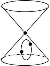
Figure 11. $\mathbb{R}A$ bounds a disc on $\mathbb{R}P(2k,1,1)$

Let us first consider the case when the double covering is equipped with the complex conjugation ${\rm conj}_{-}$; denote the covering surface by $\mathbb{C}X_{-}$. Then $p(\mathbb{R}X_{-})=\mathbb{R}P(2k,1,1)-\mbox{int}(\Delta)$. Let us denote by $P_{1}$ and $P_{2}$ the two singular points of $\mathbb{R}X_{-}$ over the two singular points of $\mathbb{C}A$. Since

$$\begin{array}[]{ll}c_{1}(\mathbb{C}X_{-})&=p^{*}\big{(}c_{1}(\mathbb{C}P(2,1,1))+\frac{1}{2}[\mathbb{C}A]\big{)}\\ &=\big{(}2+\frac{m}{2}\big{)}p^{*}(S_{\infty})+\big{(}2(k+1)+mk\big{)}p^{*}(F),\end{array}$$

$\mathbb{R}\widetilde{X}_{-}$ is orientable if and only if $4|m$.

The complex surface $\overline{P}=\mathbb{C}P(2k,1,1)/{\rm conj}$ is a $\mathbb{Q}$-homology sphere. Since the Arnold surface $\mathcal{A}=\overline{A}\cup_{\partial}c(\Delta)$ is a 2-sphere, it follows that $\overline{X}_{-}=\mathbb{C}X_{-}/{\rm conj}$ is a $\mathbb{Q}$-homology 4-sphere.

If $4|m$, the surface $\mathbb{R}X_{-}$ is an oriented surface of genus 2 with two of its nontrivial cycles pinched (see Figure 12); the two points $P_{3}$ and $P_{4}$ obtained in this way are Q-singularities with

$$[{\rm tb}_{P_{3}}]=[{\rm tb}_{P_{4}}]=\left[\!\!\begin{array}[]{rr}-\frac{2k}{4}&\frac{2k}{4}\\ \frac{2k}{4}&-\frac{2k}{4}\end{array}\right]$$

observed by Corollary 14, Section 5.

$P_{3}$                       $P_{4}$

$P_{1}$

$P_{2}$

Figure 12.

$$\begin{array}[]{ll}\mbox{Hence, \hskip 42.67912pt }0&=\big{\langle}c^{\prime}(\mathbb{R}X_{-}),c^{\prime}(\mathbb{R}X_{-})\big{\rangle}_{\overline{X}_{-}}\\ &=\sum_{i=1}^{4}\overline{{\rm tb}}_{P_{i}}(\mathbb{R}X_{-},\mathbb{R}X_{-})-2\chi(\mathbb{R}X_{-}-4\mbox{ points})\\ &=\overline{{\rm tb}}_{P_{1}}+\overline{{\rm tb}}_{P_{2}}+0+0+-2\cdot(-2-2)\\ &=\overline{{\rm tb}}_{P_{1}}+\overline{{\rm tb}}_{P_{2}}+8.\end{array}$$

The proof for the first claim now follows from Equation 2, Section 2.1.

If $m\equiv 2\mbox{ mod }4$, then $\mathbb{R}\widetilde{X}_{-}$ is not orientable. But as in the proof of Theorem 15, we observe that $\mathbb{R}X_{-}=\mathbb{R}\widetilde{X}_{-}/\widetilde{p}^{-1}(S_{\infty})$ is orientable. The two Q-singularities $P_{3}$ and $P_{4}$ obtained in this way have

$$[{\rm tb}_{P_{3}}]=[{\rm tb}_{P_{4}}]=\left[\!\!\begin{array}[]{rr}-\frac{2k}{4}&-\frac{2k}{4}\\ -\frac{2k}{4}&-\frac{2k}{4}\end{array}\right]$$

so that

$$\begin{array}[]{ll}0&=\sum_{i=1}^{4}\overline{{\rm tb}}_{P_{i}}(\mathbb{R}X_{-},\mathbb{R}X_{-})-2\chi(\mathbb{R}X_{-}-4\mbox{ points})\\ &=\overline{{\rm tb}}_{P_{1}}+\overline{{\rm tb}}_{P_{2}}+2\big{(}-\frac{k}{2}-\frac{k}{2}-\frac{k}{2}-\frac{k}{2}\big{)}+-2\cdot(-2-2)\\ &=\overline{{\rm tb}}_{P_{1}}+\overline{{\rm tb}}_{P_{2}}-8k+8\end{array}$$

completing the proof for the second claim. ∎

References

- [1] A’Campo, N.: Le groupe de monodromie du déploiement des singularités isol éées de courbes planes. I. (French) Math. Ann. 213, 1–32 (1975)
- [2] Beauville A.: Surface Algébriques Complexes, Astérisque 54, Société Mathématique de France 1978
- [3] Bennequin D.: Entrelacements et équations de Pfaff. Astérisque 107-108, 87–161 (1983)
- [4] Bredon, G.E: Introduction to compact transformation groups, Pure and Applied Mathematics, Vol. 46, New York-London: Academic Press 1972
- [5] Degtyarev A.I., Kharlamov V.M.: Topological properties of real algebraic varieties: du cot de chez Rokhlin. Russ. Math. Surv. 55 (4), 735-814 (2000)
- [6] Dimca A.: Singularities and Topology of Hypersurfaces, Springer-Verlag 1992
- [7] Durfee A.: Fifteen characterization of rational double points and simple critical points. Enseign. Math. (2) 25, no. 1-2, 131–163 (1979)
- [8] Durfee A.: The signature of smoothings of complex surface singularities. Math. Ann. 232, 85–98 (1978)
- [9] Finashin, S. M.: An integral formula for the complex intersection number of real cycles in a real algebraic variety with topologically rational singularities. (English. English, Russian summary) Zap. Nauchn. Sem. S.-Peterburg. Otdel. Mat. Inst. Steklov. (POMI) 279, Geom. i Topol. 6, 241–245, 250–251 (2001)
- [10] Finashin S. M.: Complex intersection of real cycles in real algebraic varieties and generalized Arnold-Viro inequalities. preprint, math.AG/9902022
- [11] Finashin S. M.: Rokhlin’s question and smooth quotients by complex conjugation of singular real algebraic surfaces. Topology, ergodic theory, real algebraic geometry, 109–119, Amer. Math. Soc. Transl. Ser. 2, 202, Amer. Math. Soc., Providence, RI 2001.
- [12] Gompf R.E., Stipsicz A.I.: 4-Manifolds and Kirby Calculus, Graduate Studies in Mathematics 20, AMS 1999
- [13] Gusein-Zade, S.M. Intersection matrices for certain singularities of functions of two variables. (Russian, English) Funct. Anal. Appl. 8, 10-13 (1974); translation from Funkts. Anal. Prilozh. 8, No.1, 11-15 (1974)
- [14] Harer J., Kas A., Kirby R.: Handlebody decomposition of complex surface, Memoirs AMS, No. 350, Providence, RI, USA, vol. 62 1986
- [15] Laufer H.B.: Normal Two-Dimensional Singularities, Annals of Math. Studies 71, Princeton University Press 1971
- [16] Milnor J.: Singular Points of Complex Hypersurfaces, Annals of Math. Studies 61, Princeton University Press 1968
- [17] Némethi A.: Five lectures on normal surface singularities. With the assistance of Ágnes Szilárd and Sándor Kovács. Bolyai Soc. Math. Stud., 8, Low Dimensional Topology(Eger, 1996/Budapest, 1998), 269–351, János Bolyai Math. Soc., Budapest (1999)
- [18] Orlik P., Wagreich P.: Isolated singularities of algebraic surfaces with C∗ action. Ann. of Math. 2 93, 205–228 (1971)
- [19] Öztürk F.: On Thurston-Bennequin numbers of Brieskorn double points. Proceedings of Istanbul Singularity Workshop, June 2001, to appear
- [20] Saveliev, N.: Invariants for homology 3-spheres, Encyclopaedia of Mathematical Sciences, 140, Low-Dimensional Topology, I. Berlin: Springer-Verlag 2002
- [21] Silhol R.: Real Algebraic Surfaces, Lecture Notes in Math. 1392, Berlin: Springer-Verlag 1989
- [22] Varcenko A. N.: Contact structures and isolated singularities. (Russian) Vestnik Moskov. Univ. Ser. I Mat. Mekh. 101, no. 2, 18—21 (1980)