High resolution conjugate filters for the simulation of flows

Abstract

This paper proposes a Hermite-kernel realization of the conjugate filter oscillation reduction (CFOR) scheme for the simulation of fluid flows. The Hermite kernel is constructed by using the discrete singular convolution (DSC) algorithm, which provides a systematic generation of low-pass filter and its conjugate high-pass filters. The high-pass filters are utilized for approximating spatial derivatives in solving flow equations, while the conjugate low-pass filter is activated to eliminate spurious oscillations accumulated during the time evolution of a flow. As both low-pass and high-pass filters are derived from the Hermite kernel, they have similar regularity, time-frequency localization, effective frequency band and compact support. Fourier analysis indicates that the CFOR-Hermite scheme yields a nearly optimal resolution and has a better approximation to the ideal low-pass filter than previously CFOR schemes. Thus, it has better potential for resolving natural high frequency oscillations from a shock. Extensive one- and two-dimensional numerical examples, including both incompressible and compressible flows, with or without shocks, are employed to explore the utility, test the resolution, and examine the stability of the present CFOR-Hermite scheme. Extremely small ratio of point-per-wavelength (PPW) is achieved in solving the Taylor problem, advancing a wavepacket and resolving a shock/entropy wave interaction. The present results for the advection of an isentropic vortex compare very favorably to those in the literature.

Key Words: hyperbolic conservation laws; conjugate filters; discrete singular convolution; Hermite kernel; high resolution.

I Introduction

The rapid progress in constructing high performance computers gives great impetus to the development of innovative high order computational methods for solving problems in computational fluid dynamics (CFD). With high-order numerical methods, complex flow structures are expected to be resolved more accurately in both space and time. For flow problems with sophisticate structures, high resolution is a must in order for the structural information to be correctly extracted. High order numerical resolution is of crucial importance in all kinds of simulations of turbulence. For example, direct numerical simulation (DNS) of turbulence is one of the typical situations where high resolution schemes are definitely required because the amplitude of the Fourier response of the velocity field is continuously distributed over a wide range of wavenumbers. The situation is more complex in the large eddy simulation (LES), where the energy spectrum is not only continuous, but also slow decaying at sufficiently high wavenumbers. Unlike a linear problem, the numerical error of the $q$th order finite difference scheme is not linearly scaled with the power of grid size $\Delta^{q}$. Thus numerical errors have to be strictly controlled by choosing a grid which is much smaller than the smallest spatial structure in turbulent motion[1]. The simulation become more difficult as the Reynolds number increases. For incompressible Euler flows, although the total kinetic energy is conserved, its spectral distribution of the solution could move towards the high frequency end with respect to the time evolution. As a consequence, the integration will collapse at a sufficiently long time with a finite computational grid due to the limited high frequency resolution of a given scheme. Nevertheless, a higher resolution scheme can dramatically improve the stability of the numerical iterations compared with a lower resolution one because of its ability to better resolve the high frequency components. Using three candidate schemes, i.e., a second-order finite difference scheme, a forth-order finite difference scheme and a pseudo‘spectral scheme, Browning and Kreiss[2] demonstrated that in the long-time DNS of turbulence, only the forth-order scheme can yield results comparable with those of the pseudospectral scheme.

Apart from the DNS and LES of turbulence, computational aeroacoustics (CAA) is another area where high resolution schemes are highly demanded for the simulation of waves with large spectral bandwidth and amplitude disparity[3]. For an imperfectly expanded supersonic jet, the Strouhal number ranges from $10^{-2}$ to $10^{1}$. The velocity fluctuation of the radiated sound wave can be four orders of magnitude smaller than that of the mean flow. Therefore, the real space and time numerical simulation of turbulence flow and sound wave interaction in an open area and long time process is still a severe challenge to practitioners of CAA. Obviously, high resolution schemes can be used to alleviate the demanding on a dense mesh in this situation.

The concept of high resolution is subjective. For a given scheme, it might provide a relatively high resolution for one problem but fail doing so for another problem. Yang et al[4] show that for the heat equation, a local scheme delivers higher accuracy than the Fourier pseudospectral method, while the latter achieves better accuracy in solving the wave equation. Essentially, the pseudospectral method possesses the highest numerical resolution for approximating bandlimited periodic $L^{2}$ functions. However, it might not be the most accurate method for other problems. It is noted that much argument given to the numerical resolution of computational schemes in the literature is analyzed with respect to the discrete Fourier transform. Such a resolution should be called Fourier resolution and differs much from the numerical resolution in general. It is commonly believed that a scheme of high Fourier resolution, i.e., it provides a good approximation to the Fourier transform of the derivative operators over a wider range of wavenumbers, will perform well in numerical computations. Although the results of discrete Fourier analysis might be consistent with the numerical resolution and be useful for a large class of problems, they are strictly valid only for bandlimited periodic $L^{2}$ functions. For example, the Fourier resolution of the standard finite difference schemes is not very high as given by the Fourier analysis. However, the standard finite difference schemes are the exact schemes for approximating appropriate polynomials.

There are two approaches to obtain high resolutions in a numerical computation. One is to employ a spectral method, such as the pseudospectral or Chebyshev method. In general spectral methods provide very high numerical resolution for a wide variety of physical problems. However, they often have stringent constraints on applicable boundary conditions and geometries. The other approach is to modified the coefficients of the standard finite difference scheme so that the high frequency components of a function are better approximated under the cost of the approximation accuracy for the low wavenumbers. Typical examples include the compact scheme [5] and dispersion relation preserving (DRP) scheme [6]. Fourier analysis of the both schemes indicates that they can give a better representation in a broader wavenumber range than their central difference counterparts. Therefore, they might yield a good resolution for small flow structures in a more stable manner. These modified finite difference schemes are very popular and give better numerical results for many physical problems.

The presence of shock waves adds an extra level of difficulty to the seeking of high resolution solutions. Formally, a shock will lead to a first-order error which will propagate to the region away from the discontinuity in a solution obtained by using a high order method[7]. Therefore, the attainable overall order of resolution is limited. However, for a given problem, the approximation accuracy achieved by using a high resolution scheme can be much higher than that obtained by using a low resolution scheme. In the context of shock-capturing, high resolution refers this property not only in smooth regions but also in regions as close to the discontinuity as possible. One of popular high order shock-capturing schemes is an essential non-oscillatory (ENO) scheme[8, 9, 10]. The key idea of the ENO scheme is to suppress spurious oscillations near the shock or discontinuities, while maintaining a higher-order accuracy at smooth regions. This approach was further extended into a weighted essentially non-oscillatory (WENO) scheme[11]. The WENO approach takes a linear combination of a number of high-order schemes of both central difference and up-wind type. The central difference type of schemes has a larger weight factor at the smooth region while the up-wind type of schemes plays a major role near the shock or discontinuity. The arbitrarily high order schemes which utilize the hyperbolic Riemann problem for the advection of the higher order derivatives (ADER)[12] and monotonicity preserving WENO scheme[13] are the most recent attempts in developing higher-order shock-capturing schemes. These schemes are very efficient for many hyperbolic conservation law systems.

One of the most difficult situations in the CFD is the interaction of shock waves and turbulence, which occurs commonly in high speed flows such as buffeting, air intaking and jet exhaust. Many high order shock-capturing schemes are found to be too dissipative to be applicable for the long-time integration of such flows[14, 15]. In the framework of free decaying turbulence, the effect of a subgrid-scale model was masked by some high-order shock-capturing schemes. Excessive dissipation degrades the numerical resolution and smears small-scale structures. Typically, there are two ways to reduce the excessive numerical dissipation. One is to rely on shock sensors for switching on-off dissipative terms locally. The spatial localization of the sensors is crucial to the success of the approach. In the framework of synchronization, a set of interesting nonlinear sensors was proposed[16] for achieving optimal localization automatically. The other approach is to develop low dissipation schemes, such as filter schemes. In fact, a filter, or a dissipative term, can be extracted from a regular scheme, such as the ENO. Such a term can be combined with another high-order non-dissipative scheme, such as a central difference scheme, to construct a new shock-capturing scheme [17, 18]. The overall dissipation of the new scheme can be controlled by using an appropriate switch. Numerical experiments have shown that these schemes can be of higher accuracy and less dissipative than the original shock-capturing schemes[18].

Recently, a conjugate filter oscillation reduction (CFOR) has been proposed as a nearly optimal approach for treating hyperbolic conservation laws[19, 20]. The CFOR seeks a uniform high resolution both in approximating derivatives and in filtering spurious oscillations. The conjugated filters are constructed by using the discrete singular convolution (DSC) algorithm, which provides a spectral-like resolution in a smooth region. Moreover, the accuracy of the DSC algorithm is controllable by adjusting the width of the computational support. From the point of signal processing, the DSC approximations of derivatives are high-pass filters, whereas, spurious oscillations are removed by using a conjugate low-pass filter, without resort to upwind type of dissipative terms. The low-pass and high-pass filters are conjugated in the sense that they are generated from the same DSC kernel expression. The resolution of the CFOR scheme is therefore determined by the common effective frequency band of the high-pass and low-pass filters. The effective frequency band is the wavenumber region on which both low-pass and high-pass filters have correct frequency responses. Although, the errors produced at a discontinuity are still of the first order, their absolute values are very small due the use of the high resolution CFOR scheme.

There are a variety of DSC kernels that can be used for realizing the CFOR scheme[21]. In fact, these kernels might exhibit very different characteristic in numerical computations, in particular, for shock-capturing. The latter is very sensitive to the property of DSC kernels. So far, the most widely used kernels is the regularized Shannon kernel (RSK)[19, 20]. The success of the RSK in numerical computations, particularly, in shock capturing, motivates us to search for new DSC kernels which might have more desirable features for certain aspects of shock-capturing. Indeed, Hermite kernel (HK) is a very special candidate[22, 23, 24]. Compared with the RSK, the Hermite kernel has a narrow effective frequency band but its low-pass filter better approximates the idea low-pass filter. As such, we speculate that the Hermite kernel should have a resolution similar to the RSK in the smooth flow region and might have better overall performance in the presence of shock. Extensive numerical tests are given in this paper to explore the utility and potential of the CFOR-Hermite scheme.

The rest of this paper is organized as follows. In Section II, we give a brief introduction to the DSC algorithm and Hermite kernel. The CFOR scheme based on the Hermite kernel is also described in this section. The time marching schemes are discussed. Extensive numerical results are presented in Section III to demonstrate the use of the CFOR-Hermite and to explore its resolution limit. Concluding remarks are given in Section IV.

II Theory and algorithm

This section present the spatiotemporal discretizations of a flow equation. Fourier analysis is carried out for both the low-pass and high-pass filters generated from the Hermite kernel. Time marching schemes are described after the introduction to the discrete singular convolution (DSC) and conjugate filter oscillation reduction (CFOR) scheme.

A DSC-Hermite algorithm and CFOR scheme

Discrete singular convolution (DSC) is an effective approach for the numerical realization of singular convolutions, which occurs commonly in science and engineering. The DSC algorithm has been widely used in computational science in recent years. In this section we will give a brief review on the DSC algorithm before introducing a new kernel, the Hermite kernel. For more details of the background and application of the DSC algorithm in partial difference equations, the reader is referred to Refs. [21, 24, 25, 26].

In the context of distribution theory, a singular convolution can be defined by

$$F(t)=(T*\eta)(t)=\int_{-\infty}^{\infty}T(t-x)\eta(x)dx,$$ (1)

where $T$ is a singular kernel and $\eta(x)$ is an element of the space of test functions. Interesting examples include singular kernels of Hilbert type, Abel type and delta type. The former two play important roles in the theory of analytical functions, processing of analytical signals, theory of linear responses and Radon transform. Since delta type kernels are the key element in the theory of approximation and the numerical solution of differential equations, we focus on the singular kernels of delta type

$$T(x)=\delta^{(q)}(x),~{}~{}~{}~{}(q=0,1,2,\cdots),$$ (2)

where superscript $(q)$ denotes the $q$th-order “derivative” of the delta distribution, $\delta(x)$, with respect to $x$, which should be understood as generalized derivatives of distributions. When $q=0$, the kernel, $T(x)=\delta(x)$, is important for the interpolation of surfaces and curves, including applications to the design of engineering structures. For hyperbolic conservation laws and Euler systems, two special cases, $q=0$ and $q=1$ are involved, whereas for the full Naiver-Stokes equations, the case of $q=2$ will be also invoked. Because of its singular nature, the singular convolution of Eq. (1) cannot be directly used for numerical computations. In addition, the restriction to the test function is too strict for most practical applications. To avoid the difficulty of using singular expressions directly in numerical computations, we consider a sequence of approximations of the form

$$\lim_{\alpha\rightarrow\alpha_{0},{\rm or}\beta\rightarrow\beta_{0},\cdots}\delta^{(q)}_{\alpha,\beta,\cdots}(x)=\delta^{(q)}(x),~{}~{}~{}~{}(q=0,1,2,\cdots),$$ (3)

where ${\alpha,\beta,\cdots}$ are a family of parameters which characterize the approximation and ${\alpha_{0},\beta_{0}}$ are generalized limits. At least one of the parameters in Eq. (3) has to take a limit. One of the most commonly used DSC kernels is the regularized Shannon kernel (RSK)

$$\delta_{\sigma,\Delta}(x-x_{k})={\sin{\pi\over\Delta}(x-x_{k})\over{\pi\over\Delta}(x-x_{k})}\exp\left({(x-x_{k})^{2}\over 2\sigma^{2}}\right),$$ (4)

where $\Delta$ is the grid spacing and $\sigma$ characterizes width of the Gaussian envelop. The regularity of the kernel approximation can be improved by using a Gaussian regularizer. Obviously, for a given $\sigma\neq 0$, the limit of $\Delta\rightarrow 0$ reproduces the delta distribution. Numerical approximation to a function $f$ (low-pass filtering) and its $q$th derivative (high-pass filtering) are realized by the following discrete convolution algorithm

$$f^{(q)}(x)\approx\sum_{k=-W}^{W}\delta^{(q)}_{\sigma,\Delta}(x-x_{k})f(x_{k}),\quad(q=0,1,2,\cdots),$$ (5)

where $\{x_{k}\}_{k=-W}^{W}$ are a set of discrete grid points which are centered at $x$, and $2W+1$ is the computational bandwidth, or effective kernel support, which is usually smaller than the entire computational domain.

In this work, we consider the Hermite function expansion of the delta distribution[22, 23, 24]

$$\delta_{\sigma,\Delta}(x-x_{k})=\frac{1}{\sigma}\mbox{exp}\left(-\frac{(x-x_{k})^{2}}{2\sigma^{2}}\right)\sum_{k=0}^{n/2}\left(-\frac{1}{4}\right)^{k}\frac{1}{\sqrt{2\pi}k!}H_{2k}\left(\frac{x-x_{k}}{\sqrt{2}\sigma}\right),$$ (6)

where $H_{2k}(x)$ is the usual Hermite polynomial. The delta distribution is recovered by taking the limit $n\rightarrow\infty$. The Hermite function expansion of the Dirac delta distribution was proposed by Korevaar[22] over forty years ago and was considered by Hoffman et. al. for wave propagations[23]. Further discussion of its connections to wavelets and the DSC algorithm can be found in Ref. [24](b). Just like other DSC kernels, the expression (6) is a low-pass filter, see FIG. 7. Its approximation to the idea low-pass filter is effectively controlled by the parameter $\sigma$. The $q$th order derivative is readily given by the analytical differentiation of expression (6) with the use of recursion relations

$$H_{k}^{(2)}(x)-2xH^{(1)}_{k}(x)+2kH_{k}(x)=0;$$ (7)

$$H^{(1)}_{k}(x)=2kH_{k-1}(x).$$ (8)

In numerical applications, optimal results are usually obtained if the Gaussian window size $\sigma$ varies as a function of the central frequency $\pi/\Delta$, such that $r=\sigma/\Delta$ is a parameter chosen in computations. In FIG. 7, we plot the frequency responses of both the regularized Shannon kernel (RSK) and Hermite kernel (HK). It is seen that the effective frequency band of the RSK is slightly wider than that of the HK. The most distinctive difference of these two kernels occurs in their low-pass filters. Compared with the RSK, the HK low-pass filters decay fast at high wavenumbers and thus better approximate the ideal low-pass filter. As a result, they are expected to remove high-frequency errors much more efficiently. The ramification of these differences in numerical computations is examined extensively in the next section.

The essence of the CFOR scheme is the following. Since the DSC high-pass filters have a limited effective frequency band, short wavelength numerical errors will be produced when these high-pass filters are used for numerical differentiations. Conjugate low-pass filters are designed to remove such errors. The resulting solution should be reliable over the effective frequency band, i.e., the low wavenumber region on which both high-pass and low-pass filters are very accurate. A total variation diminishing (TVD) switch is used to activate the low-pass filter whenever the total variation of the approximate solution exceeds a prescribed criteria. By adjusting the parameter $r$ in the low-pass filter which determines the effective frequency band with a given DSC kernel, the oscillation near the shock can be reduced efficiently. Since the DSC-Hermite kernel is nearly interpolative, the low-pass filter in the CFOR scheme is implemented via prediction ($u(x_{i})\rightarrow u(x_{i+\frac{1}{2}})$) and restoration ($u(x_{i+\frac{1}{2}})\rightarrow u(x_{i})$) [19, 20]. The CFOR scheme with the RSK has been successfully applied to a variety of standard problems, such as inviscid Burgers’ equation, Sod and Lax problems, shock-tube problems, flow past a forward facing step and the shock/entropy wave interaction[19, 20].

B Time marching schemes

In this work, we study four types of systems: 2D incompressible Euler system, 1D linear advective equation, 1D compressible Euler system and 2D compressible Euler system. For the incompressible Euler system, we adopt a third-order Runge-Kutta scheme, where a potential function is introduced to update the pressure in each stage and the bi-conjugate gradient method is used to solve the Poisson equation of the potential function for the pressure difference. More detail of the scheme can be found Ref. [26, 27]. For all the other systems, a standard forth-order Runge-Kutta scheme is employed for time integrations.

The choice of the time increment needs special care to assure that the solution is not only stable but also time accurate. To ensure the iteration of the 2D incompressible Naiver-Stokes system to be stable under a third-order Runge-Kutta scheme, the following CFL condition should be satisfied [10]

$$\Delta t\left[\underset{i,j}{\mbox{max}}\left(\frac{|u_{ij}|}{\Delta x}+\frac{|v_{ij}|}{\Delta y}\right)+\frac{2}{\mbox{Re}}\left(\frac{1}{\Delta x^{2}}+\frac{1}{\Delta y^{2}}\right)\right]\leq 1.$$ (9)

For the time integration of the linear advection equation, Hu et al [28] demonstrated that a stricter restraint should be posed on $\Delta t$ to guarantee the solution to be time accurate. In this work, we test the numerical resolution of the proposed CFOR-Hermite scheme by using different small time increments $\Delta t$ to ensure the overall numerical error is dominated by the spatial discretization.

III Numerical Experiments

In this section, a few benchmark numerical problems, including, the incompressible 2D Euler flow, a 1D wave equation, 1D and 2D compressible Euler systems, are employed to test shock-capturing capability of the proposed CFOR-Hermite scheme and to examine the numerical resolution of the scheme. We choose the CFOR-Hermite parameters of $n=88$ and $W=32$ for all the computations. The parameter of $r=3.05$ is used for high-pass filtering and the prediction. For restoration, $r<3.05$ is used.

Example 1. Taylor problem

As a benchmark test, the Taylor problem governed by the 2D incompressible Navier-Stokes equations is commonly used to access the accuracy and stability of schemes in CFD[10, 27]. The extension of this problem to the test of resolution can be found in Ref. [4]. Since the viscous term leads to the dissipation of the initial wave, the long-time evolution accuracy of a numerical scheme can be masked by the viscous decay. In the present computation, we consider the incompressible Euler version of this problem, i.e. Taylor problem without the viscous term.

With a periodic boundary condition, the 2D time dependent incompressible Euler equation admits the following exact solution

$$u(x,y,t) = -\mbox{cos}(kx)\mbox{sin}(ky)$$ (10)

$$v(x,y,t) = \quad\mbox{sin}(kx)\mbox{cos}(ky)$$ (11)

$$p(x,y,t) = -\left(\mbox{cos}(2kx)+\mbox{cos}(2ky)\right)/4.0,$$ (12)

where $u,v,p$ denote the velocity in $x$- and $y$-directions and the pressure, respectively. Here $k$ is the wavenumber of the velocity solution. Note that the wavenumber of the pressure is twice as much as that of the velocity. Therefore, for a given $k$ value, the overall accuracy is limited by the capability of resolving the pressure. The computation domain is chosen as $[0,2\pi]\times[0,2\pi]$ with periodic boundary conditions in both directions. Mesh size of the computational domain is $1/N$, and $N=64$ is used in all the tests in this problem. We examine the resolution of the CFOR scheme with a variety of $k$ values. The numerical errors with respect to the exact velocity $u$ are listed in Table VIII, whereas the ratio of grid points per wavelength (PPW) is computed according to the pressure wavenumber ($2k$). The PPW is a good measure of the numerical resolution for many problems of wave nature. Comparison is also carried out between the regularized Shannon kernel (RSK) and the Hermite kernel, since we speculate that for this smooth problem the RSK should have a better performance with a high wavenumber due to its wider effective frequency band as shown in FIG. 7.

The results in Table VIII exhibit high accuracy of the DSC algorithm, realized both by the RSK and HK. It is not surprising that with the increase of the wavenumber $k$, the accuracy of the numerical scheme degrades due to the finite effective frequency band. In FIG. 7, we analyze the Fourier resolution of the RSK and HK (the stars) against the Fourier response of the exact solution with a given $k$ (the straight lines). Their relative locations in the Fourier domain tell us the approximation errors. The accuracy of the final results is eventually limited by the Fourier resolution, i.e., the effective frequency band of the kernel. First, we note that results in Table VIII are qualitatively consistent with the analysis in FIG. 7. For example, the analysis indicates that the RSK has a better Fourier resolution than the RK. The numerical results in Table VIII show the same tendency. Quantitatively, the frequency response error of the first order derivative approximated by using the RSK is about $10^{-10}$ at wavenumber $2k=26$. The errors of numerical results are also about $5\times 10^{-11}$ and thus match the Fourier analysis. In general, there is a good consistence between the prediction of Fourier analysis and the experimental results for the RSK. In a dramatic case, the PPW ratio is reduced to 2.1, which is very close to the Nyquist limit of 2. It is noted that the CFOR-RSK still performs very well for this case. This confirms the spectral nature of the CFOR-RSK scheme.

For the Hermite kernel, the errors at $2k=20$ and 26 are slightly smaller than those predicted by the Fourier analysis. This discrepancy is due to the fact that the actual errors measured are for the velocity rather than for the pressure. The pressure error might not fully propagate to the velocity because only the pressure gradient contributes to velocity changes. Comparing with the RSK, the Hermite kernel has a narrow effective frequency band, and thus performs not as well as the RSK. However, a careful examination on the FIG. 7 reveals that the Hermite kernel has a sharp decay in its conjugate low-pass filter as the wavenumber increases. Therefore, it is expected to perform better in the case of shock-capturing involving natural high frequency oscillations. This is indeed the case as demonstrated in the example of shock/entropy wave interaction.

Example 2. Double shear layers

This problem is also governed by the 2D incompressible Euler equations with periodic conditions[10]. The problem is not analytically solvable due to the following initial conditions

$$u(x,y,t) = \begin{cases}\mbox{tanh}\left(\frac{2y-\pi}{2\rho}\right),&\mbox{if}~{}y\leq\pi\\ \mbox{tanh}\left(\frac{3\pi-2y}{2\rho}\right),&\mbox{if}~{}y>\pi\end{cases}$$ (13)

$$v(x,y,t) = \delta\mbox{sin}(x),$$ (14)

where, $\rho$ represents the thickness of the shear layer. Such initial conditions describe a thin horizontal shear layer disturbed by a small vertical velocity. The initial flow quickly evolves into roll-ups with smaller and smaller scales until the full resolution is lost[10]. A small $\rho$ speeds up the formation of small-scale roll-ups. The initial shear layers become discontinuous as $\rho$ approaches zero. In order to resolve the fine structures of roll-ups, high-order schemes are necessary. However, the use of high-order schemes along is not sufficient for achieving high resolution. The shock-capturing ability is required for solving this problem. Bell, Colella and Glaz[29] introduced a second order Godunov-type shock-capturing scheme to simulate this incompressible flow. E and Shu[10] considered an ENO scheme for handling this case. Recently, Liu and Shu[30] applied a discontinuous Galerkin method to this problem. In the present work, we examine the performance of the CFOR-Hermite scheme for this problem. The low-pass filter will be activated whenever spurious oscillations are generated from the flow fields. The parameter $r=2.6$ is used in the restoration.

We consider the case of $\rho=1/15$ and $\delta=0.05$ in our simulation. The time increment is fixed as $0.002$ and a mesh of $64^{2}$ is used. We note that a finer mesh was considered in previous work[29, 10, 30]. One of our objectives is to demonstrate that the CFOR gives excellent results with a coarse mesh.

FIG. 7 depicts the velocity contours at $t=4,6,8$ and 10. It is seen that very good resolution is obtained in such a coarse grid. The present results are very smooth and the integration is very stable. Spurious oscillations are effectively removed by the conjugate low-pass filter. There is no serious distortion occurring to the channels connecting individual vorticity centers. It is worthwhile to stress that if a numerical scheme is highly dissipative, the vorticity cores which should be skew circle shape (see FIG. 7 for cases $t=4,6$) will be smeared to a circle shape. The quality of the present solution at early times is comparable to that of the spectral solution given by E and Shu[10].

Example 3. Advective sine-Gaussian wavepacket

This 1D problem is designed to examine the resolution of the CFOR-Hermite approach with a linear advection equation $\frac{\partial u}{\partial t}+c\frac{\partial u}{\partial x}=0$ with a smooth solution. In this problem, the initial data is taken as a wavepacket constructed by using a Gaussian envelop modulated by a sine wave with a wavenumber $k$

$$u(x,t=0)=\mbox{sin}[2\pi k(x-x_{0})]e^{\frac{(x-x_{0})^{2}}{\sigma^{2}}}$$ (15)

where $x_{0}$ is the center of the wavepacket, initially located in the $x=0$. The parameter $\sigma$ is chosen such that tail of the wavepacket will be small enough inside the domain. In present study, we choose $\sigma=\sqrt{2}/10$. The computational domain is set to [-1,1] with periodic boundary conditions. If $c=1$, the configuration of the initial wavepacket repeats itself every 2 time units. We consider a variety of wavenumbers $k$ to explore the resolution limit of the present CFOR-Hermite scheme. The mesh size is chosen as $1/N$ while $N=100$. Two time increments are selected to ensure that the time discretization error is negligible. As our scheme is extremely accurate, it requires a very small time increment to fully demonstrate its machine precision when $k=5$. Both the exact solution and numerical approximation at $t=100$ are plotted in FIG. 7 for a comparison. Obviously, there is no visual difference between them. Our results are listed in Tables VIII and VIII for a quantitative evaluation. For a large $k$ value, the wavepacket is highly oscillatory. It is a challenge for a low resolution scheme to resolve the advective wave. We explore the limitation of the present scheme by choosing a variety of $k$ values. The performance of the CFOR-Hermite scheme can be well predicted by the Fourier analysis as shown in FIG. 7. It is noted that the Fourier transform of a Gaussian is still a Gaussian. The accuracy of the results is limited by the Fourier resolution of the Hermite differentiation, whose errors are indicated in FIG. 7 for a number of different wavenumbers. For example, the case with $k=20$ is safely located to the left of the $\Delta\omega=10^{-10}$, which is the error of the differentiation. As a result, the CFOR error for the case of $k=20$ is of the order of $10^{-10}$ or less, with a small time increment. However, for the case of $k=30$, its Gaussian tail is truncated by the limit $\Delta\omega=10^{-4}$. Consequently, the highest accuracy can not exceed this limitation, even with a small time increment.

The long time behavior of the CFOR-Hermite scheme for this problem is presented in Table VIII. We integrate the system as long as 100 time units to investigate the reliability of the present approach for some large $k$ values ($k=20$ and 25). The corresponding PPW values are 5 and 4 respectively. Both the long time stability and numerical resolution demonstrated in this problem are very difficult for most existing shock-capturing schemes to achieve.

Example 4. Advective 2D isentropic vortex

In this case, an isentropic vortex is introduced to a uniform mean flow, by small perturbations in velocity, density and the temperature. These perturbations involve all the three types of waves, i.e., vorticity, entropy and acoustic waves. The background flow and the perturbation parameters are given, respectively by

$$(u_{\infty},v_{\infty},p_{\infty},T_{\infty})=(1,1,1,1),$$ (16)

and

$$u^{\prime}=-\frac{\lambda}{2\pi}(y-y_{0})e^{\eta(1-r^{2})},$$ (18)

$$v^{\prime}=\frac{\lambda}{2\pi}(x-x_{0})e^{\eta(1-r^{2})},$$ (19)

$$T^{\prime}=-\frac{(\gamma-1)\lambda^{2}}{16\eta\gamma\pi^{2}}e^{2\eta(1-r^{2})},$$ (20)

where $r=\sqrt{(x-x_{0})^{2}+(y-y_{0})^{2}}$ is the distance to the vortex center, $\lambda=5$ is the strength of the vortex and $\eta$ is a parameter determining the gradient of the solution, and is unity in this study. By the isentropic relation, $p=\rho^{\gamma}$ and $T=p/\rho$, the perturbation in $\rho$ is required to be

$$\rho=(T_{\infty}+T^{\prime})^{1/(\gamma-1)}=\left[1-\frac{(\gamma-1)\lambda^{2}}{16\eta\gamma\pi^{2}}e^{2\eta(1-r^{2})}\right]^{1/(\gamma-1)}.$$ (21)

The governing equation is the compressible Euler equations with periodic boundary conditions[18]. This problem was considered to measure the formal order and the stability in long-time integrations of many high order schemes[18] because it is analytically solvable.

To be consistent with the literature[18], we chose a computational domain of $[0,10]\times[0,10]$ with the initial vortex center located at $(5,5)$. Our results are tabulated in Tables VIII and VIII. Results of many standard schemes[18] are also listed in these tables for a comparison. To be consistent with Ref. [18] the error measures used in this problem are defined as

$$L_{1} = {1\over(N+1)^{2}}\sum_{i=0}^{N}\sum_{j=0}^{N}|f_{i,j}-\bar{f}_{i,j}|$$ (22)

$$L_{2} = {1\over(N+1)}\left[\sum_{i=0}^{N}\sum_{j=0}^{N}|f_{i,j}-\bar{f}_{i,j}|^{2}\right]^{1\over 2},$$ (23)

where $f$ is the numerical result and $\bar{f}$ the exact solution. Note that these definitions differ from the standard ones used in other problems. In Ref. [18], the CFL=0.5 was used and was nearly optimal. In our computation, the optimal time increment is much smaller because the nature of high resolution. We have set CFL=0.01 in some of our computations to release the full potential of the present scheme. It is noted that there is a dramatic gain in the accuracy as the mesh is refined from $40\times 40$ to $80\times 80$. The numerical order reaches 15 indicating that the proposed scheme is of extremely high order. The present results obtained at the $80^{2}$ mesh are about $400$ times more accurate than those of other standard schemes obtained at $320^{2}$. Therefore, by using the present approach, a dramatical reduction of the mesh size and computing time can be gained for 3D large scale computations.

The stability of the time integration is another useful test for numerical schemes. We choose a mesh of $80\times 80$ to test the accuracy at long time computations with CFL=0.5. Although the time increment is not optimal for present scheme, practical computations usually require the time increment to be as large as possible, especially for long time integrations. Numerical solutions are sampled at $t=2,10,50$ and 100. To prevent the numerical errors from their nonlinear growth, the conjugate low-pass filter is activated to stabilize the computation. This problem differs from the advective sine-Gaussian wavepacket, where the equation is linear and the growth of the numerical error is fairly slow. The superior stability of the present CFOR scheme can be observed from Table VIII and FIG. 7. Even at $t=100$, the accuracy is still extremely high and the vortex core is well preserved.

Example 5. Shock/entropy wave interaction

To further examine the resolution of the CFOR-Hermite scheme in the presence of shock waves, the interaction of shock/entropy waves is employed. In this case, small amplitude, low-frequency entropy waves are produced in the upstream of a shock. After the interaction with the shock, these waves are compressed in frequency and amplified in the amplitude. This is a standard test problem for high-order shock-capturing schemes and its governing equation is the compressible Euler system[9]. A linear analysis can be used to estimate the wave amplitude after the shock, which depends only on the shock strength and the amplitude before the shock. Therefore, the performance of a shock-capturing scheme can be evaluated by checking against the linear analysis. Low order methods perform poorly due to the oscillatory feature of the compressed waves. The ratio of frequencies before and after the shock depends only on the shock strength. The problem is defined in a domain of [0,5] and with following initial conditions[9]

$$(\rho,u,p)=\left\{\begin{array}[]{lcrl}(3.85714,&2.629369,&10.33333);&x\leq 0.5\\ (e^{-\epsilon\sin(\kappa x)},&0,&1.0);&x>0.5\\ \end{array}\right.,$$ (26)

where $\epsilon$ and $\kappa$ are the amplitude and wavenumber of the entropy wave before the shock. These initial conditions represent a Mach 3 shock. We fix the amplitude of the wave $\epsilon$ before the shock to be 0.01. Accordingly the amplitude after the shock is determined to be 0.08690716 by the linear analysis. In our previous study[20], the CFOR-RSK scheme was successfully applied to this problem. Here we focus on the resolution of the Hermite kernels. A variety of pre-shock wavenumbers $\kappa$ are considered for this purpose and the corresponding parameters are summarized in Table VIII. Uniform meshes with grid spacing $1/N$ and $r=2.55$ are used for all the cases and their entropy waves are plotted in FIG. 7.

The entropy waves after the shock are well predicted in all the test cases, as indicated by the fully developed amplitude of entropy waves after the shock. A low order scheme or a scheme with excessive dissipation will lead to dramatical damping of the entropy waves. For $\kappa$=13, a mesh of $N=400$ is enough to well resolve the problem. When such a mesh is used in case of $\kappa=26$, the resolution is still very good. On a refined mesh $N=800$, the $\kappa=26$ case is better resolved as shown in FIG. 7(d). In our previous test using the CFOR-RSK scheme, the case of $\kappa=52$ was quite difficult to resolve on the mesh of $N=800$. Such a difficulty is postponed in the present CFOR-Hermite scheme. The entropy waves of the case $\kappa=52$ with $N=800$ are plotted in FIG. 7(e), where the resolution is very good. Obviously, the good performance of the present CFOR-Hermite is attributed to its fast decay feature of the low-pass filter in its Fourier frequency response, see FIG. 7. When a finer mesh of $N=1200$ is used for the case of $\kappa=52$, the quality of the solution near the shock front improves remarkably. Keeping the PPW being 5, a mesh of $N=1000$ is used for the case of $\kappa=65$ and results with high resolution are obtained, as shown in FIG. 7(g). It can be noted that there is a slight over-dumping at the tail of the generated entropy waves and a remarkable improvement is achieved as the mesh is refined from $N=1000$ to $N=1200$, see FIG. 7(h). As the last example, the case of $\kappa=70$ is considered on the same mesh. Obviously, the CFOR-Hermite scheme yields a good solution for such a high wavenumber too. To our knowledge, such a high resolution has not been reported in the literature yet.

IV Conclusion Remarks

This paper introduces the conjugate filter oscillation reduction (CFOR) scheme with a Hermite kernel for the numerical simulation of both incompressible and compressible flows. The CFOR-Hermite scheme is based on a discrete singular convolution (DSC) algorithm, which is a potential approach for the computer realization of singular convolutions. In particular, the DSC algorithm provides accurate approximations for spatial derivatives, which are high-pass filters form the point view of signal processing, in the smooth region of the solution. Therefore, the DSC algorithm makes it possible to resolve complex flow structures with a very small ratio of point-per-wavelength (PPW) in fluid dynamical simulations. The essential idea of the CFOR scheme is that, a similar high-resolution low-pass filter which is conjugated to the high-pass filters will be activated to eliminate high-frequency errors whenever the spurious oscillation is generated in the flow for whatever reasons. The conjugate low-pass and high-pass filters are nearly optimal for shock-capturing and spurious oscillation suppression in the sense that they are generated from the same expression and consequently have similar order of regularity, effective frequency band and compact support.

An efficient and flexible DSC kernel plays a key role in the present CFOR scheme for resolving problems involving sharp gradients or shocks. Fourier analysis is conducted for both regularized Shannon kernel (RSK) and Hermite kernel. A comparison of both kernels reveals that the RSK has a wider effective frequency band for its high-pass filters, whereas the Hermite kernel gives a better approximation to the idea low-pass filter. As a consequence, the DSC-RSK scheme achieves a better PPW ratio for flows without spurious oscillations, while the proposed CFOR-Hermite scheme performs better for shock-capturing with natural high frequency oscillations. The effective frequency bands of both kernels are much wider than those of most prevalent spatial discretization schemes.

Extensive numerical examples are employed to access the accuracy, test the stability, demonstrate the usefulness and most importantly, examine the resolution of the present CFOR-Hermite scheme. Our test cases cover four types of flow systems: 2D incompressible Euler systems, 1D linear advective equation, 2D compressible Euler systems and 1D shock/entropy wave interaction. Comparison is made between the RSK and Hermite kernel for the 2D incompressible flow. The DSC-RSK scheme performs better than the DSC-Hermite for smooth initial values. The capability of the CFOR-Hermite scheme for flow simulations is illustrated by a variety of test examples. It is about $10^{5}$ times more accurate than some popular shock-capturing schemes in the advancement of a 2D isentropic vortex flow. Its advantage over the CFOR-RSK scheme is exemplified in predicting the shock/entropy wave interaction, where reliable results are attained at about 5 PPW. Such a small ratio indicates that the present CFOR-Hermite has a great potential for being used for large scale computations with a very small mesh to achieve a given resolution.

Acknowledgment

This work was supported in part by the National University of Singapore.

Error	Kernel	$k$(PPW)
		1(32)	2(16)	5(6.4)	10(3.2)	13(2.5)	15(2.1)
$L_{2}$	Hermite	6.63E-15	9.53E-15	2.45E-14	6.74E-13	1.01E-5	-
	RSK	4.88E-15	3.55E-15	1.96E-14	1.47E-12	5.89E-11	1.55E-3
$L_{\infty}$	Hermite	2.78E-15	4.66E-15	1.86E-14	5.26E-13	4.79E-6	-
	RSK	2.33E-15	3.55E-15	1.64E-14	9.69E-13	4.19E-11	8.37E-4

TABLE I.: $L_{2}$ and $L_{\infty}$ errors of Taylor problem with Hermite kernel and RSK at $t=2$. The PPW ratio in the bracket is calculated according to the wavenumber of the pressure.

Time	$k$(PPW)
	5(20)	10(10)	15(6.7)	20(5)	25(4)	30(3.3)
2	2.00E-11	3.47E-10	2.26E-9	9.01E-9	3.34E-8	4.71E-5
4	4.01E-11	6.95E-10	4.53E-9	1.80E-8	6.68E-8	9.41E-5
6	6.01E-11	1.04E-9	6.79E-9	2.70E-8	1.00E-7	1.41E-4
8	8.02E-11	1.39E-9	9.06E-9	3.60E-8	1.34E-7	1.88E-4
10	1.00E-10	1.74E-9	1.13E-8	4.51E-8	1.67E-7	2.35E-4

TABLE II.: $L_{1}$ error for the advective sine-Gaussian wavepacket, $\Delta t=10^{-4}$.

Time	$k$(PPW)
	5(20)	10(10)	15(6.7)	20(5)	25(4)	30(3.3)
2	1.17E-14	4.77E-14	4.23E-14	5.86E-12	2.21E-8	4.70E-5
4	2.11E-14	8.86E-14	8.23E-14	1.17E-11	4.43E-8	9.41E-5
6	2.46E-14	1.36E-13	1.11E-13	1.76E-11	6.64E-8	1.41E-4
8	3.19E-14	1.79E-13	1.46E-13	2.35E-11	8.86E-8	1.88E-4
10	4.01E-14	2.27E-13	1.73E-13	2.93E-11	1.11E-7	2.36E-4

TABLE III.: $L_{1}$ error for the advective sine-Gaussian wavepacket, $\Delta t=5\times 10^{-6}$.

Time		10	20	50	80	100
$L_{1}$	$k$=20	4.51E-8	9.01E-8	2.25E-7	3.60E-7	4.51E-7
	$k$=25	1.67E-7	3.34E-7	8.35E-7	1.34E-6	1.67E-6
$L_{\infty}$	$k$=20	2.78E-7	5.56E-7	1.39E-6	2.22E-6	2.78E-6
	$k$=25	1.51E-6	3.02E-6	7.55E-6	1.21E-5	1.51E-5

TABLE IV.: Errors for the advective sine-Gaussian wavepacket in long-time integrations.

N		CFOR1	CFOR2	C4	ENO	MUSCL	WENO	ENOACM	MUSCLACM	WENOACM
40	error	2.37E-5	6.45E-6	1.13E-3	1.28E-3	2.39E-3	9.39E-4	7.81E-4	1.29E-3	6.11E-4
80	error	4.73E-9	2.79E-10	5.78E-5	2.08E-4	5.99E-4	7.07E-5	6.68E-5	2.79E-4	4.58E-4
	order	12.29	14.50	4.29	2.62	1.99	3.73	3.55	2.19	3.74
160	error	3.34E-10	3.76E-11	3.79E-6	3.01E-5	1.26E-4	2.46E-6	7.84E-6	5.31E-5	2.95E-6
	order	3.82	2.89	3.93	2.79	2.25	4.84	3.09	2.40	3.97
320	error	5.12E-11	3.20E-11	2.41E-7	4.07E-6	2.26E-5	8.52E-8	6.82E-7	8.61E-6	2.13E-7
	order	2.71	0.23	3.97	2.89	2.47	4.85	3.52	2.62	3.79

TABLE V.: $L_{1}$ error for the density at $t=2$; The CFL number is 0.01 for CFOR² and 0.5 for all the other schemes; C4: fourth-order accurate, conservative centered scheme; ENO: third-order; MUSCL: third-order; WENO: fifth-order; XXX^ACM denotes that the C4 scheme is used as the basic scheme with the XXX being a characteristic-based filter, while Harten’s artificial compression method is used as a sensor to indicate the local numerical dissipation, see Ref. [18].

N		CFOR1	CFOR2	C4	ENO	MUSCL	WENO	ENOACM	MUSCLACM	WENOACM
40	error	4.35E-5	1.80E-5	2.92E-3	4.09E-3	8.29E-3	3.16E-3	2.47E-3	4.05E-3	2.08E-3
80	error	1.41E-8	1.06E-9	1.90E-4	6.75E-4	2.26E-3	2.64E-4	2.08E-4	1.14E-3	1.48E-4
	order	11.59	14.05	3.94	2.60	1.88	3.58	3.57	1.83	3.81
160	error	1.03E-9	4.73E-10	1.23E-5	8.69E-5	5.91E-4	1.10E-5	2.51E-5	3.12E-4	9.44E-6
	order	3.78	1.16	3.95	2.96	1.94	4.58	3.05	1.87	3.97
320	error	4.14E-10	4.08E-10	7.84E-7	1.33E-5	1.31E-4	2.93E-7	2.19E-6	6.07E-5	6.85E-7
	order	1.31	0.21	3.97	2.71	2.17	5.23	3.52	2.36	3.78

TABLE VI.: $L_{2}$ error for the density at $t=2$. See Table VIII for captions.

Time	2	10	50	100
$L_{1}$	4.73E-9	1.23E-8	4.58E-8	1.05E-7
$L_{2}$	1.41E-8	3.64E-8	1.41E-7	3.17E-7

TABLE VII.: Errors for the density at different times (CFL=0.5, N=80).

Case No.	1	2	3	4	5	6	7	8	9
$k$	13	13	26	26	52	52	65	65	70
N	400	800	400	800	800	1200	1000	1200	1200
PPW	10	20	5	10	5	7.5	5	6	5.58

TABLE VIII.: A summary of test cases for the shock/entropy wave interaction.

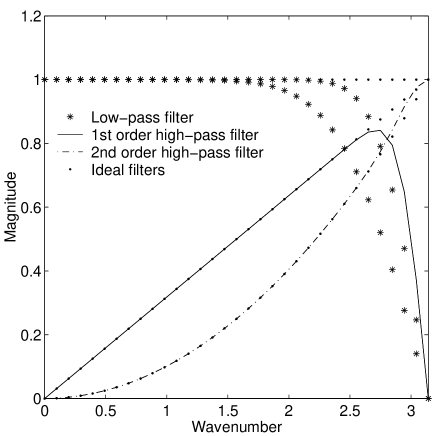
(a) RSK

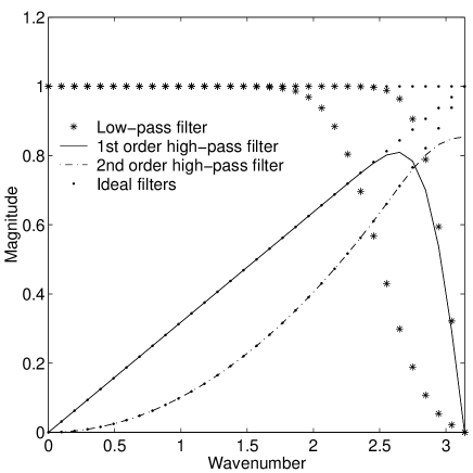
(b) HK

FIG. 1.: Frequency responses of the conjugate DSC filters (in the unit of $1/\Delta$), The maximum amplitude of the filters is normalized to the unit. For HK: $W$=32; $r$=3.05 for high-pass filters; $r$=2.5 for the left low-pass filter; $r$=3.05 for the right low-pass filter. For RSK: $W$=32; $r$=5.4 for high-pass filters; $r$=2.0 for the left low-pass filter; $r$=3.2 for the right low-pass filter.

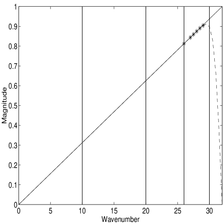
(a) RSK

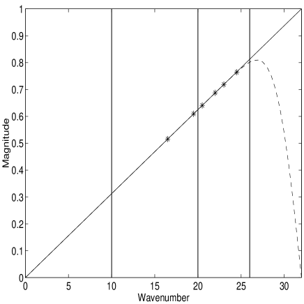
(b) HK

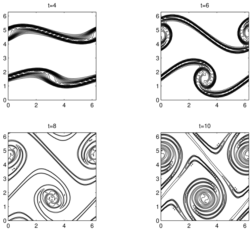
FIG. 2.: Fourier analyses for the Taylor problem. Wavenumbers are rescaled such that the maximum is the half of mesh number, i.e., 32 unit length. Sharp peaks are 1D projections of frequency responses of the exact solutions. Six stars indicate the critical wavenumber beyond which $\Delta\omega$, will be greater than $10^{-10},10^{-7},10^{-6},10^{-5},10^{-4},10^{-3}$, respectively (from the left to the right). Here, $\Delta\omega$ is the difference between the exact first-order derivative (the diagonal line) and the kernel approximation (the dashed line).

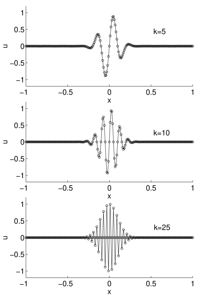
FIG. 3.: Contours of vorticity for double shear layer problem at different time.

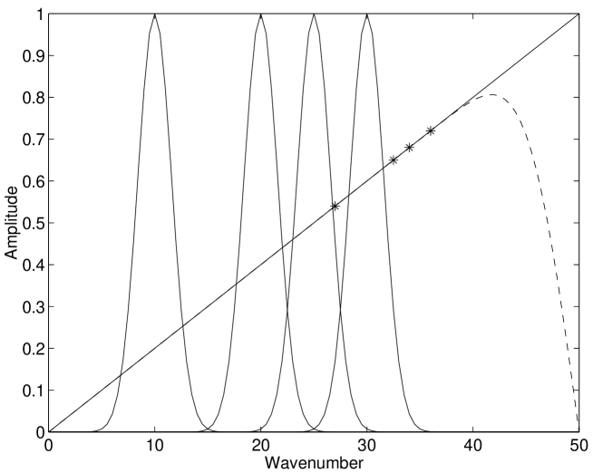
FIG. 4.: The sine-Gaussian wavepackets at $t=100$. Exact solutions are plotted in solid lines and numerical ones are given by circles.

FIG. 5.: Fourier analyses for the advective sine-Gaussian wavepacket. Wavenumbers are rescaled such that the maximum is the half of mesh number, i.e., 50 unit length. Four Gaussian peaks correspond to $k=10,20,25,30$, respectively. Four stars indicate the critical wavenumbers beyond which $\Delta\omega$ will be greater than $10^{-10},10^{-6},10^{-5},10^{-4}$, respectively (from the left to the right). Here, $\Delta\omega$ is the difference between the exact first-order derivative (the diagonal line) and the kernel approximation (the dashed line).

(a) $t=2$

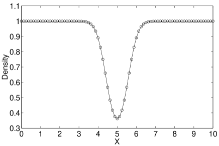
(b) $t=10$

(c) $t=50$

(d) $t=100$

FIG. 6.: Density profiles in horizontal cutting at four times. Solid line is the exact profile and the circle dots denote the numerical results. $N=80$; CFL=0.5. See also the Table VIII for numerical errors.

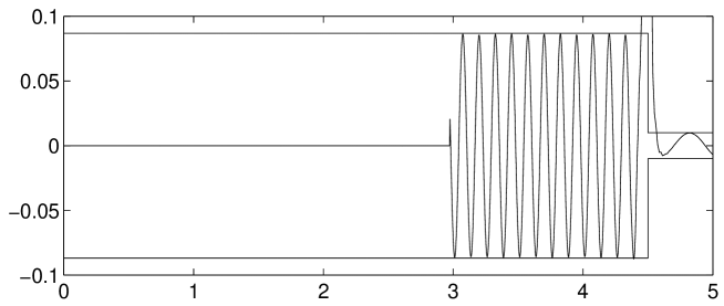
(a) $k=13,N=400$

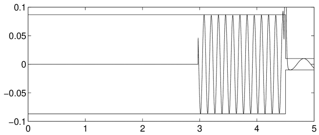
(b) $k=13,N=800$

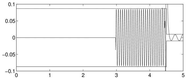
(c) $k=26,N=400$

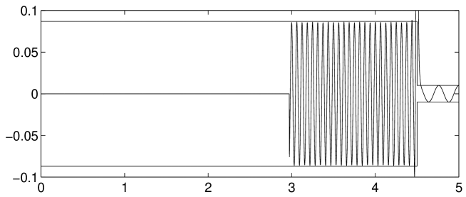
(d) $k=26,N=800$

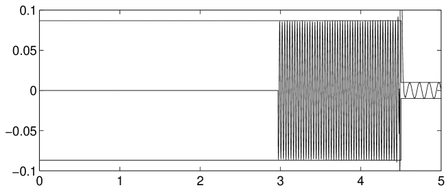
(e) $k=52,N=800$

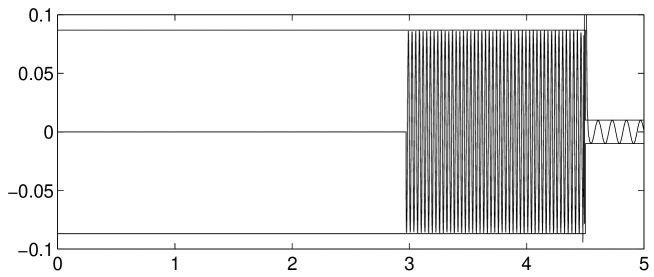
(f) $k=52,N=1200$

(g) $k=65,N=1000$

(h) $k=65,N=1200$

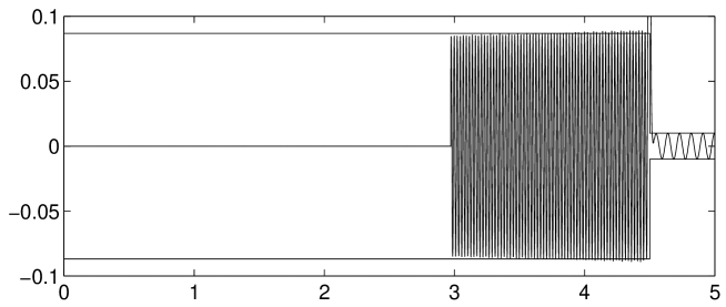
(i) $k=70,N=1200$

FIG. 7.: Entropy waves for different pre-shock wavenumber.

REFERENCES

- [1] S. Ghosal, An analysis of numerical errors in large-eddy simulations of turbulence, J. Comput. Phys. 125, 187-206 (1996).
- [2] G. L. Browning and H.-O. Kreiss, Comparison of numerical methods for the calculation of two-dimensional turbulence, Math. Comput. 186, 389-410 (1989).
- [3] C. K. W. Tam, Computational aeroacoustics: issues and methods, AIAA Journal, 13(10), 1788-1796 (1995).
- [4] S. Y. Yang, Y. C. Zhou and G. W. Wei, Comparison of the discrete singular convolution algorithm and the Fourier pseudospectral method for solving partial differential equations, Comput Phys. Commun. in press.
- [5] S. K. Lele, Compact finite difference scheme with spectral-like resolution, J. Comput. Phys. 103, 16-42 (1992).
- [6] C. K. W. Tam and J. C. Webb, Dispersion-relation-preserving finite difference schemes for Computational Acoustics, J. Comput. Phys. 107, 262-281 (1993).
- [7] B. Engquist and B. Sjögreen, Examples of error propagation from discontinuities, Barriers and Challenges in Computational Fluid Dynamics, edited by V. Venkatakrishnan, Manuel D. Salas and Sukumar R. Chakravarthy (Boston, MA : Kluwer Academic Publishers, 1998), p. 27.
- [8] A. Harten, B. Engquist, S. Osher and S. Chakravarthy, Uniform high-order accurate essentially non-oscillatory schemes, III, J. Comput. Phys. 71, 231-303 (1987).
- [9] C.-W. Shu, Essentially non-oscillatory and weighted essentially non-oscillatory schemes for hyperbolic conservation laws, ICASE Report, No. 97-65, (1997).
- [10] W. E and C.-W. Shu, A numerical resolution study of high order essentially non-oscillatory schemes applied to incompressible flow, J. Comput. Phys. 110, 39-46 (1994).
- [11] X.-D. Liu, S. Osher, and T. Chan, Weighted essentially non-oscillatory schemes, J. Comput. Phys. 115, 200-212 (1994).
- [12] E. F. Toro, R. C. Millington and V. A. Titarev, ADER: arbitrary-order non-oscillatory advection scheme, Proc. 8th International Conference on Non-linear Hyperbolic Problems, Magdeburg, Germany, March, 2000.
- [13] D. S. Balsara and C.-W. Shu, Monotonicity preserving weighted essentially non-oscillatory Schemes with Increasingly High Order of Accuracy, J. Comput. Phys. 160, 405-452 (2000).
- [14] S. Lee, S. K. Lele and P. Moin, Interaction of isotropic turbulence with shock waves: Effect of shock strength, J. Fluid Mech. 340, 225-247 (1997).
- [15] E. Garnier, M. Mossi, P. Sagaut, P. Comet and M. Deville, On the use of shock-capturing scheme for large-eddy simulation, J. Comput. Phys. 153, 273-311 (2001).
- [16] G. W. Wei, Synchronization of single-side averaged coupling and its application to shock capturing, Phys. Rev. Lett. 86, 3542-3545 (2001).
- [17] H. C. Yee, N. D. Sandham and M. J. Djomehri, Low-dissipative high-order shock-capturing methods using characteristic-based filters, J. Comput. Phys. 150, 199-238 (1999).
- [18] E. Garnier, P. Sagaut and M. Deville, A class of explicit ENO filters with application to unsteady flows, J. Comput. Phys. 170, 184-204 (2001).
- [19] G. W. Wei, and Y. Gu, Conjugated filter approach for solving Burgers’ equation, J. Comput. Appl. Math. revised. arXiv:math.SC/0009125, Sept. 13, (2000).
- [20] Y. Gu and G. W. Wei, Conjugated filter approach for shock capturing, submitted.
- [21] G. W. Wei, Discrete singular convolution for the solution for the Fokker-Planck equations, J. Chem. Phys. 110, 8930-8942 (1999).
- [22] J. Korevaar, Pansions and the theory of Fourier transforms, Amer. Math. Soc. Trans. 91, 53-101 (1959).
- [23] D. K. Hoffman, N. Nayar, O. A. Sharafeddin and D. J. Kouri, Analytic banded approximation for the discretized free propagator, J. Phys. Chem. 95, 8299-8305 (1991).
- [24] G. W. Wei, Wavelets generated by using discrete singular convolution kernels, J. Phys. A, Mathematical and General, 33, 8577-8596 (2000).
- [25] G. W. Wei, A new algorithm for solving some mechanical problems, Comput. Methods Appl. Mech. Engng. 190, 2017-2030 (2001).
- [26] D.C. Wan, B. S. V. Patnaik and G. W. Wei, A new benchmark quality solution for the buoyancy driven cavity by discrete singular convolution, Numer. Heat Transfer B - Fundamentals, 40, 199-228 (2001).
- [27] D. C. Wan and Y. C. Zhou and G. W. Wei, Numerical solution of incompressible flows by discrete singular convolution, Int. J. Numer. Meth. Fluid. in press.
- [28] F. Q. Hu, M. Y. Hussaini and J. Manthey, Low-dissipation and -dispersion Runge-Kutta schemes for computational acoustic, NASA TR-94-102.
- [29] J. B. Bell, P. Colella and H. M. Glaz, A 2nd-order projection method for the incompressible Navier Stokes equations, J. Comput. Phys. 85, 257-283 (1989).
- [30] J.-G. Liu and C.-W. Shu, A high-order discontinuous Galerkin method for 2D incompressible flows, J. Comput. Phys. 160, 577-596 (2000).