A global stability criterion for scalar functional differential equations

Abstract

We consider scalar delay differential equations $x^{\prime}(t)=-\delta x(t)+f(t,x_{t})\ (*)$ with nonlinear $f$ satisfying a sort of negative feedback condition combined with a boundedness condition. The well known Mackey-Glass type equations, equations satisfying the Yorke condition, and equations with maxima all fall within our considerations. Here, we establish a criterion for the global asymptotical stability of a unique steady state to $(*)$. As an example, we study Nicholson’s blowflies equation, where our computations support the Smith’s conjecture about the equivalence between global and local asymptotical stabilities in this population model.

1 Introduction

We start by considering the simple autonomous linear equation

$$x^{\prime}(t)=-\delta x(t)+ax(t-h),$$ (1)

governed by friction ($\delta\geq 0$) and delayed negative feedback ($a<0$). Necessary and sufficient conditions for the asymptotic stability of (1) are well known [5]. For example, in the simplest case $\delta=0$, Eq. (1) is asymptotically stable if and only if $-ah\in(0,\pi/2)$. If we allow for a variable delay in (1), we obtain the equation

$$x^{\prime}(t)=-\delta x(t)+ax(t-h(t)),\ 0\leq h(t)\leq h,$$ (2)

whose stability analysis is more complicated than that of the autonomous case. Nevertheless several sharp stability conditions were established for Eq. (2). The first of them is due to Myshkis (see [5, p. 164]) and it states that in the case $\delta=0$ the inequality $-a\sup_{\mathbb{R}}h(t)<3/2$ guarantees the asymptotic stability in (2). This condition is sharp (this fact was established by Myshkis himself). In particular, the upper bound $3/2$ can not be increased to $\pi/2$. Later on, the result by Myshkis has been improved by different authors, the most celebrated extensions are due to Yorke [17] and Yoneyama [16] (both for $\delta=0$). Finally, the Myshkis condition has been recently generalized [6] for $\delta>0$: Eq. (2) is asymptotically stable if

$$-\frac{\delta}{a}\exp{(-h\delta)}>\ln\frac{a^{2}-a\delta}{\delta^{2}+a^{2}}.$$ (3)

We note that for every fixed $a,\delta$ and $h>0$ condition (3) is sharp, and in the limit case $\delta=0$ it coincides with the Myshkis condition. Here the sharpness means that if $a,\delta,h$ do not satisfy (3), then the asymptotic stability of Eq. (2) can be destroyed by an appropriate choice of a periodic delay $h(t)$ (see [6, Theorem 4.1]). Returning to Eq. (1), we can observe that (3) approximates exceptionally well the exact stability domain for (1) given in [5]: see Fig. 1, where the domains of local (dashed line) and global (solid line) stability are shown in coordinates $(-a/\delta,\exp(-\delta h))$. When $\delta=0$, we obtain $3/2$ as an approximation for $\pi/2$.

It is a rather surprising fact that the sharp global stability condition (3) works not only for linear equations, but as well for a variety of nonlinear delay differential equations of the form

$$x^{\prime}(t)=-\delta x(t)+f(t,x_{t}),\ \ (x_{t}(s)\stackrel{{\scriptstyle def}}{{=}}x(t+s),\ s\in[-h,0]),$$ (4)

where $f:\mathbb{R}\times{\mathcal{C}}\to\mathbb{R}$, ${\mathcal{C}}\stackrel{{\scriptstyle def}}{{=}}C[-h,0],$ is a measurable functional satisfying the additional condition (H) given below. Due to the rather general form of (H), Eq. (4) incorporates, possibly after some transformations, some of the most celebrated delay equations, such as equations satisfying the Yorke condition [17], equations of Wright [5, 8], Lasota-Wazewska, and Mackey-Glass [2, 7, 10], and equations with maxima [6, 11]. Solutions to some of these equations can exhibit chaotic behavior so that the analysis of their global stability is of great importance –at least on the first stage of the investigation (see [7, p.148] for further discussion). As an example, in Section 2 we consider Nicholson’s blowflies equation, for which our computations support the conjecture of Smith posed in [14].

Let us explain briefly the nature of our further assumptions. In part, they are motivated by the sharp stability results for (4) obtained in [17] ($\delta=0$) and [6] ($\delta>0$) under the assumption that for some $a<0$ and for all $\phi\in{\mathcal{C}}$, the following Yorke condition holds:

$$a\mathcal{M}(\phi)\leq f(t,\phi)\leq-a\mathcal{M}(-\phi).$$ (5)

Here $\mathcal{M}:{\mathcal{C}}\to\mathbb{R}$ is the monotone continuous functional (sometimes called the Yorke functional) defined by $\mathcal{M}(\phi)=\max\{0,\max_{s\in[-h,0]}\phi(s)\}$. In general, $f$ satisfying (5) is nonlinear in $\phi$. On the other hand, in some sense it has a “quasi-linear” form (for example, $f(\phi)=\max_{s\in[-h,0]}\phi(s)$ can be written as $f(\phi)=\phi(-s_{\phi})$). In particular, $f$ is sub-linear in $\phi$, which makes impossible the application of the results from [6, 17] to the strongly nonlinear cases such as the celebrated Wright equation

$$x^{\prime}(t)=a(1-\exp(-x(t-h))),\ a<0,$$ (6)

which is also globally asymptotically stable if $-ah\in(0,3/2)$. Roughly speaking, the Yorke $3/2$-stability condition does not imply the Wright $3/2$-stability result. Our recent studies [8] of (6) revealed the following interesting fact: the essential feature of the function $f(x)=a(1-\exp(-x)))$ in (6) allowing the extension of the Wright $3/2$-stability result to some other nonlinearities is the position of the graph of $f$ with respect to the graph of the rational function $r(x)=ax/(1+bx)$ which coincides with $f$, $f^{\prime}$ and $f^{\prime\prime}$ at $x=0$. This suggests the idea to consider a “rational in $\mathcal{M}$” version of the “linear in $\mathcal{M}$” condition (5) to manage the strongly nonlinear cases of (4). Therefore, we will assume the following conditions (H):

(H1)

$f:\mathbb{R}\times{\mathcal{C}}\to\mathbb{R}$ satisfies the Carathéodory condition (see [5, p.58]). Moreover, for every $q\in\mathbb{R}$ there exists  $\vartheta(q)\geq 0$ such that $f(t,\phi)\leq\vartheta(q)$ almost everywhere on $\mathbb{R}$ for every $\phi\in C$ satisfying the inequality $\phi(s)\geq q,s\in[-h,0]$.

(H2)

There are $b\geq 0,\ a<0$ such that

$$f(t,\phi) \ \geq\ \frac{a\mathcal{M}(\phi)}{1+b\mathcal{M}(\phi)}\ {\rm for\ all\ }\phi\in{\mathcal{C}};$$ (7)

$$f(t,\phi) \ \leq\ \frac{-a\mathcal{M}(-\phi)}{1-b\mathcal{M}(-\phi)}{\rm\ for\ all\ }\phi\in{\mathcal{C}}{\rm\ such\ that\ }\min_{s\in[-h,0]}\phi(s)>-b^{-1}\in[-\infty,0).$$ (8)

(H) is a kind of negative feedback condition combined with a boundedness condition; they will cause solutions to remain bounded and to tend to oscillate about zero. Furthermore, (H) implies that $x=0$ is the unique steady state solution for Eq. (4) with $\delta>0$. On the other hand, (H) does not imply that the initial value problems for (4) have a unique solution. In any case, the question of uniqueness is not relevant for our purposes. Notice finally that if (H2) holds with $b=0$ (which is precisely (5)), then (H1) is satisfied automatically with $\vartheta(q)=-aM(-q)$.

Now we are ready to state the main result of this work:

Theorem 1.

Assume that (H) holds and let $x:[\alpha,\omega)\to\mathbb{R}$ be a solution of (4) defined on the maximal interval of existence. Then $\omega=+\infty$ and $x$ is bounded on $[\alpha,+\infty)$. If, additionally, condition (3) holds, then $\lim_{t\to+\infty}x(t)=0$. Furthermore, condition (3) is sharp within the class of equations satisfying (H): for every triple $a<0,\ \delta>0,\ h>0$ which do not meet (3), there is a nonlinearity $f$ satisfying (H) and such that the equilibrium $x(t)=0$ of the corresponding Eq. (4) is not asymptotically stable.

It should be noticed that in this paper we do not consider the limit cases when $b=0$ and/or $\delta=0$. When $b=0,\delta>0$, Theorem 1 was proved in [6, Theorem 2.9]. The limit case $\delta=0,\ b\geq 0$ can be addressed by adapting the proofs in [8]. Here, due to the elimination of the friction term $-\delta x$, an additional condition is necessary (see [9] for details). In this latter case, (3) takes the limit form $-ah\in(0,3/2)$.

Remark 1.1.

The set of four parameters ($h>0,\delta>0,a<0,b>0$) can be reduced. Indeed, the change of time $\tau=\delta t$ transforms (4) into the same form but with $\delta=1$. Finally, since $\mathcal{M}$ is a positively homogeneous functional ($\mathcal{M}(k\phi)=k\mathcal{M}(\phi)$ for every $k\geq 0$, $\phi\in{\mathcal{C}}$), and since the global attractivity property of the trivial solution of (4) is preserved under the simple scaling $x=b^{-1}y$, the exact value of $b>0$ is not important and we can assume that $b=1$. Also, the change of variables $x=-y$ transforms (4) into $y^{\prime}(t)=-\delta y(t)+[-f(t,-y_{t})]$ so that it suffices that at least one of the two functionals $f(t,\phi),-f(t,-\phi)$ satisfy (7) and (8).

To prove Theorem 1, in Sections 3 and 4 we will construct and study several one-dimensional maps which inherit the stability properties of Eq. (4). The form of these maps depends strongly on the parameters: in fact, we will split the domain of all admissible parameters given by (3) into several disjoint parts and each one-dimensional map will be associated to a part. Some of the maps are rather simple and an elementary analysis is sufficient to study their stability properties. Some other maps are more complicated: for example, the proof of Lemma 11 involves the concept of Schwarz derivative, whose definition and several of its properties are recalled below. Unfortunately, several important one-dimensional maps appear in an implicit form and though this form may be simple, its analysis requires considerable effort. For the convenience of the reader, the hardest and most technical parts of our estimations are placed in an appendix (Section 6). In Section 2, we will show the significance of the hypotheses (H) again by applying Theorem 1 to the well-known Nicholson blowflies equation.

2 On the Smith conjecture and equations with non-positive Schwarzian

2.1 A global stability condition

In this section we will apply our results to the delay differential equation

$$N^{\prime}(u)=-\delta N(u)+pN(u-h)e^{-\gamma N(u-h)},\ h>0,$$ (9)

used by Gurney et al. (see [14, p. 112]) to describe the dynamics of Nicholson’s blowflies. Here $p$ is the maximum per capita daily egg production rate, $1/\gamma$ is the size at which the population reproduces at its maximum rate, $\delta$ is the per capita daily adult death rate, $h$ is the generation time and $N(u)$ is the size of population at time $u.$ In view of the biological interpretation, we only consider positive solutions of (9). If $p\leq\delta,$ Eq. (9) has only one constant solution $x\equiv 0.$ For $p>\delta,$ the equation has an unstable constant solution $x\equiv 0$ and a unique positive equilibrium $N^{*}=\gamma^{-1}\ln(p/\delta)$. Global stability in Eq. (9) (when all positive solutions tend to the equilibrium $N^{*}$) has been studied by various authors by using different methods (see [2, 3, 14] for more references). Nevertheless, the exact global stability condition was not found. In this aspect, the work [14], where the conjecture about the equivalence between local and global asymptotic stabilities for Eq. (9) was posed (see [14, p. 116]), is of special interest for us. Indeed, an application of our main result to (9) strongly supports this conjecture, showing a surprising proximity between the boundaries of local and global stability domains; see Fig. 1 and the following proposition:

Theorem 2.

The positive equilibrium $N^{*}$ of Nicholson’s blowflies equation (9) is globally asymptotically stable if either $c\in(-1,0]$ or

$$\mathbf{\theta}>c\ln[(c^{2}+c)/(c^{2}+1)]\,,\,c>0,$$ (10)

where $\mathbf{\theta}=\exp(-\delta h)\,,\,c=\ln(p/\delta)-1.$

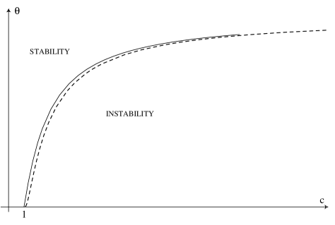
Fig. 1: Domains of global and local stability in coordinates $(c,\theta)$, $c=-a/\delta$, $\theta=\exp(-\delta h)$.

It follows from the observation given below (3) that condition (10) is sharp within the class of equations $N^{\prime}(u)=-\delta N(u)+pN(u-\rho(u))e^{-\gamma N(u-\rho(u))}$ with variable delay $\rho:\mathbb{R}\to[0,h]$.

As it can be seen from (10), not all parameters are independent in (9). Indeed, if we set $\tau=h\delta,u=t/\delta,q=p/\delta,x(t)=\gamma N(u)$, then (9) takes the form

$$x^{\prime}(t)=-x(t)+g(x(t-\tau)),$$ (11)

where $g(x)=qx\exp(-x)$. For every $q>1$, it has a unique positive equilibrium $x(t)\equiv\ln q$, which is globally asymptotically stable if $\ln(q)\leq 2$ (see [3]). The change of variables $x(t)=\ln q+y(t)$ reduces Eq. (11) to the equation $y^{\prime}(t)=-y(t)+w(y(t-\tau)),$ where $w(y)=(y+\ln q)e^{-y}-\ln q$. In Section 5, we will show that the nonlinearity $w(y)$ satisfies the following conditions (W) within some domain which attracts all nonnegative solutions of (11):

1. $w\in C^{3}(\mathbb{R},\mathbb{R})$,  $xw(x)<0$ for $x\neq 0$ and $w^{\prime}(0)<0$.

2. $w$ is bounded below and has at most one critical point $x^{*}\in\mathbb{R}$ which is a local extremum.

3. The Schwarz derivative $(Sw)(x)=w^{\prime\prime\prime}(x)(w^{\prime}(x))^{-1}-(3/2)\left(w^{\prime\prime}(x)(w^{\prime}(x))^{-1}\right)^{2}$ of $w$ is nonnegative: $(Sw)(x)\leq 0$ for all $x\neq x^{*}$.

Since $w^{\prime}(0)=\ln(e\delta/p)<0$ and $w^{\prime\prime}(0)>0$ if $\ln q>2$, Theorem 2 is a consequence of the following results:

Lemma 3.

[8] Let $w$ meet conditions (W) and $w^{\prime\prime}(0)>0$. Then the functional $f(t,\phi)=w(\phi(-h))$ satisfies hypotheses (H) with $a=w^{\prime}(0)$ and $b=-w^{\prime\prime}(0)/(2w^{\prime}(0))$.

Corollary 4.

Suppose that $w$ satisfies (W) and $w^{\prime\prime}(0)>0$. If (3) holds with $a=w^{\prime}(0)$, then the trivial steady state attracts all solutions of the delay differential equation

$$x^{\prime}(t)=-\delta x(t)+w(x(t-h)),\ \delta>0.$$ (12)

Corollary 4 can be applied in a similar way to obtain global stability conditions for the positive equilibrium of other delay differential equations arising in biological models. For example, we can mention the celebrated Mackey-Glass equation proposed in 1977 to model blood cell populations (see, e.g., [10]), which is of the form (12) with $w(x)=b/(1+x^{n})$, $b>0$, $n>1$. Another important model that can be considered within our approach is the Wazewska-Czyzewska and Lasota equation describing the erythropoietic (red-blood cell) system. In this case $w(x)=b_{1}\exp(-b_{2}x),\ b_{i}>0$.

As it was proved in [8], the conclusion of Corollary 4 also holds for $\delta=0$ by replacing (3) with its limit form $-ah\leq 3/2$. In the particular case of the Wright equation, this result coincides with the $3/2$- stability theorem by Wright (see [8] for more details).

2.2 The Smith and Wright conjectures revisited

Let us look again on Fig. 1, which shows the boundaries of the domains of local and global asymptotic stability for the Nicholson equation; this observation (as well as Proposition 8 stated below) suggests the following

Conjecture 2.1.

Under conditions (W), the trivial solution of Eq. (12) is globally attracting if it is locally asymptotically stable.

An interesting particularity of Conjecture 2.1 is that it coincides with the celebrated Wright conjecture if we take $\delta=0,\ w(x)=a(1-\exp(-x)),$ and it coincides with the Smith conjecture if we take Nicholson’s blowflies equation.

Now, the following result was obtained in [15] as a simple consequence of an elegant approach toward stable periodic orbits for Eq. (12) with Lipschitz nonlinearities:

Proposition 5.

[15] For every $\alpha\geq 0$ there exists a smooth strictly decreasing function $w$ satisfying (W1), (W2), $-w^{\prime}(0)=\alpha$ and such that Eq. (12) has a nontrivial periodic solution which is hyperbolic, stable and exponentially attracting with asymptotic phase (so therefore (12) is not globally stable).

Proposition 5 shows clearly that the strong dependence between local (at zero) and global asymptotical stabilities of Eq. (12) cannot be explained only with the concepts presented in (W1), (W2). We notice here that the condition of negative Schwarz derivative in Eq. (12) appears naturally also in some other contexts of the theory of delay differential equations, see e.g. [10, Sections 6–9], where it is explicitly used, and [5, Theorem 7.2, p. 388], where the condition $Sw<0$ is implicitly required.

3 Preliminary stability analysis of Eq. (4)

Throughout the paper, in view of Remark 1.1, we assume that $\delta=1$ in (4) and $b=1$ in (7), (8). Hence, with $\theta\stackrel{{\scriptstyle def}}{{=}}\exp(-h)$, (3), (4), (7) and (8) take, respectively, the forms

$$-\theta/a > \ln\frac{a^{2}-a}{a^{2}+1};$$ (13)

$$x^{\prime}(t) = -x(t)+f(t,x_{t});$$ (14)

$$f(t,\phi) \geq r(\mathcal{M}(\phi)),\ {\rm for\ all\ }\phi\in{\mathcal{C}};$$ (15)

$$f(t,\phi) \leq r(-\mathcal{M}(-\phi)),{\rm\ for\ all\ }\phi\in{\mathcal{C}}{\rm\ such\ that\ }\min_{s\in[-h,0]}\phi(s)>-1,$$ (16)

where the rational function $r(x)=ax/(1+x)$ will play a key role in our constructions. In this section, we establish that the “linear” approximation to (13) of the form

$$\quad-\theta/a>-(a+1)/(a^{2}+1)$$ (17)

implies the global stability of Eq. (14) (note here that $\ln(1+x)<x$ is true for $x>0$).

In the sequel we will use some properties of the Schwarz derivative. The following lemma can be checked by direct computation:

Lemma 6.

If $g$ and $f$ are functions which are at least $C^{3}$ then $S(f\circ g)(x)=(g^{\prime}(x))^{2}(Sf)(g(x))+(Sg)(x)$. As a consequence, the inverse $f^{-1}$ of a smooth diffeomorphism $f$ with $Sf>0$ has negative Schwarzian: $Sf^{-1}<0$.

We will also need the following lemma from [13]:

Lemma 7.

[13, Lemma 2.6] Let $q:[\alpha,\beta]\to[\alpha,\beta]$ be a $C^{3}$ map with $(Sq)(x)<0$ for all $x$. If $\alpha<\gamma<\beta$ are consecutive fixed points of some iteration $g=q^{N}$ of $q$, $N\geq 1,$ and $[\alpha,\beta]$ contains no critical point of $g$, then $g^{\prime}(\gamma)>1$.

This lemma allows us to prove the following proposition, which plays a central role in our analysis.

Proposition 8.

Let $q:[\alpha,\beta]\to[\alpha,\beta]$ be a $C^{3}$ map with a unique fixed point $\gamma$ and with at most one critical point $x^{*}$ (maximum). If $\gamma$ is locally asymptotically stable and the Schwarzian derivative $(Sq)(x)<0$ for all $x\not=x^{*}$, then $\gamma$ is the global attractor of $q$.

Proof.

Let $W$ be the connected component of the open set $S=\{x\in[\alpha,\beta]\,:\,\lim_{k\to+\infty}q^{k}(x)=\gamma\}$ which contains $\gamma$. Clearly, $g(W)\subset W$. If $W\neq[\alpha,\beta]$, then we have three possibilities: $W=[\alpha,r)$, $W=(l,\beta]$ or $W=(l,r)$, $\alpha<l<r<\beta$.

If $W=[\alpha,r)$ then $q(r)=\lim_{\epsilon\to 0+}q(r-\epsilon)\leq r\leq q(r)$, a contradiction with the fact that $q$ does not have fixed points in $[\alpha,\beta]$ different from $\gamma$. The case $W=(l,\beta]$ is completely analogous.

In the case $W=(l,r)$, by the same arguments, it should hold $q(l)=r$, $q(r)=l$. Thus $l<\gamma<r$ are consecutive fixed points of $g=q^{2}$ and $g^{\prime}(\gamma)=(q^{\prime}(\gamma))^{2}\leq 1$. By Lemma 7, $x^{*}\in(l,r)$ and therefore $q(x^{*})<r$. Since $q$ has a maximum at $x^{*}$, $r>q(x^{*})\geq q(l)$, a contradiction.

Hence $W=[\alpha,\beta]$ and therefore $\{\gamma\}$ attracts each point of $[\alpha,\beta]$. This implies that $\gamma$ is the global attractor of $q$ (see [4, Chapter 2]). ∎

Now we are in a position to begin the stability analysis of Eq. (14).

Lemma 9.

Suppose that (H) holds and let $x:[\alpha-h,\omega)\to\mathbb{R}$ be a solution of Eq. (14) defined on the maximal interval of existence. Then $\omega=+\infty$ and $M=\limsup_{t\to\infty}x(t),\ m=\liminf_{t\to\infty}x(t)$ are finite. Moreover, if $m\geq 0$ or $M\leq 0$, then $M=m=\lim_{t\to\infty}x(t)=0$.

Proof.

Note that (15) implies that $f(t,\phi)\geq a$ for all $t\in\mathbb{R}$ and $\phi\in{\mathcal{C}}$. Next, if $q\leq x_{\alpha}(s)\leq Q,\ s\in[-h,0]$ then for all $t\in[\alpha,\omega)$, we have

$$x(t) = \exp(-(t-\alpha))x(\alpha)+\int^{t}_{\alpha}\exp(-(t-s))f(s,x_{s})ds$$

$$\geq a+(\min\{q,a\}-a)\exp(-(t-\alpha))\geq\min\{q,a\}.$$

Next, (H1) implies that $f(s,x_{s})\leq\vartheta(\min\{q,a\})$ for all $s\geq\alpha$, so that

$$x(t)\leq\max\{Q,0\}+\vartheta(\min\{q,a\}),\ t\in[\alpha,\omega).$$

Hence $x(t)$ is bounded on the maximal interval of existence, which implies the boundedness of the right hand side of Eq. (14) along $x(t)$. Thus $\omega=+\infty$ due to the corresponding continuation theorem (see [5, Chapter 2]).

Next, suppose, for example, that $M=\limsup_{t\to\infty}x(t)\leq 0$. Thus we have $\lim\limits_{t\to\infty}\mathcal{M}(x_{t})=0$ so that, in virtue of (15), $f(t,x_{t})\geq\inf\limits_{s\geq t}a\mathcal{M}(x_{s})/(1+\mathcal{M}(x_{s}))\stackrel{{\scriptstyle def}}{{=}}a(t)$ where $a:[\alpha,+\infty)\to(-\infty,0]$ is nondecreasing and continuous, with $\lim_{t\to+\infty}a(t)=0$. Thus, by (3), $x(t)\geq\exp(-(t-\beta))x(\beta)+a(\beta)$ for all $t\geq\beta>\alpha$. This implies that $m=\liminf_{t\to\infty}x(t)=0$ so that $M=0$. ∎

Lemma 10.

Suppose that (H) holds and let $x:[\alpha-h,\infty)\to\mathbb{R}$ be a solution of Eq. (14). If $x$ has a negative local minimum at some point $s>\alpha$, then $\mathcal{M}(x_{s})>0$. Analogously, if $x$ has a positive local maximum at $t>\alpha$, then $\mathcal{M}(-x_{t})>0$.

Proof.

If $x(u)\leq 0$ for all $u\in[s-h,s]$, then $x^{\prime}(s)\geq-x(s)+r(\mathcal{M}(x_{s}))>0$, a contradiction. The other case is similar. ∎

Lemma 11.

Suppose that (H) holds and let $x:[\alpha-h,\infty)\to\mathbb{R}$ be a solution of Eq. (14). If (17) holds then $\lim_{t\to\infty}x(t)=0$.

Proof.

Let $M=\limsup_{t\to\infty}x(t),\ m=\liminf_{t\to\infty}x(t)$. In view of Lemma 9, we only have to consider the case $m<0<M$, since otherwise ($m\geq 0$ or $M\leq 0$) we have a non oscillatory solution to Eq. (14), which tends to zero as $t\to+\infty$. Thus in the sequel we will only consider the oscillating solutions $x(t)$. In this case there are two sequences of points $t_{j},s_{j}$ of local maxima and local minima respectively such that $x(t_{j})=M_{j}\to M,x(s_{j})=m_{j}\to m$ and $s_{j},t_{j}\to+\infty$ as $j\to\infty$.

First we prove that $M=m=0$ if $a(1-\theta)>-1$. Indeed, for each $s_{j}$ we can find $\varepsilon_{j}\to 0+$ such that $0<\mathcal{M}(x_{s})<M+\varepsilon_{j}$ for all $s\in[s_{j}-h,s_{j}]$. Next, by Lemma 10, there exists $h_{j}\in[0,h]$ such that $x(s_{j}-h_{j})=0$. Therefore, by the variation of constants formula,

$$m_{j}=\int_{s_{j}-h_{j}}^{s_{j}}e^{s-s_{j}}f(s,x_{s})ds\geq\int_{s_{j}-h_{j}}^{s_{j}}e^{s-s_{j}}r(\mathcal{M}(x_{s}))ds\geq r(M+\varepsilon_{j})(1-\theta).$$

As a limit form of this inequality, we get $m\geq r(M)(1-\theta)$. Hence $m>-1$ and we can use (16) for $\phi=x_{t}$ with sufficiently large $t$. Thus, in a similar way, we obtain that

$$M_{j}=\int_{t_{j}-h^{*}_{j}}^{t_{j}}e^{s-t_{j}}f(s,x_{s})ds\leq\int_{t_{j}-h^{*}_{j}}^{t_{j}}e^{s-t_{j}}r(-\mathcal{M}(-x_{s}))ds\leq r(m-\varepsilon^{*}_{j})(1-\theta)$$

for some sequences $\varepsilon^{*}_{j}\to 0+$ and $h^{*}_{j}\in[t_{j}-h,t_{j}]$. Hence we obtain $M\leq r(m)(1-\theta)\leq r(r(M)(1-\theta))(1-\theta)$. This gives $M^{2}\leq M(a(1-\theta)-1)$ which is only possible when $M=0$.

Now, assume that $a(1-\theta)\leq-1$. Since $m\geq r(M)(1-\theta)>a$ (see the first part of the proof), we conclude that $r^{-1}(m)=m/(a-m)>0$ is well defined. Next, for $s_{j}$ we can find a sequence of positive $\epsilon_{j}\to 0$ such that $m_{j}<m+\epsilon_{j}<0$. We claim that $x(s_{j}-h_{j})\geq r^{-1}(m+\epsilon_{j})$ for some $h_{j}\in[0,h]$. Indeed, in the opposite case, $x(s)<r^{-1}(m+\epsilon_{j})$ for all $s$ in some open neighborhood of $[s_{j}-h,s_{j}]$. Thus $f(s,x_{s})\geq r(\mathcal{M}(x_{s}))>m+\epsilon_{j}$ for all $s$ close to $s_{j}$. Finally, $x^{\prime}(s)>-x(s)+m+\epsilon_{j}>0$ almost everywhere in some neighborhood of $s_{j}$, contradicting the choice of $s_{j}$.

Next, there exists a sequence of positive $\epsilon^{*}_{j}\to 0$ such that $x(s)<M+\epsilon^{*}_{j}$ for all $s\in[s_{j}-h,s_{j}].$ Therefore, by the variation of constants formula,

$$m_{j} = x(s_{j})=e^{-h_{j}}x(s_{j}-h_{j})+\int_{s_{j}-h_{j}}^{s_{j}}e^{s-s_{j}}f(s,x_{s})ds$$

$$\geq e^{-h_{j}}r^{-1}(m+\epsilon_{j})+\int_{s_{j}-h_{j}}^{s_{j}}e^{s-s_{j}}r(\mathcal{M}(x_{s}))ds$$

$$\geq e^{-h_{j}}r^{-1}(m+\epsilon_{j})+r(M+\epsilon^{*}_{j})(1-e^{-h_{j}})\geq\theta r^{-1}(m+\epsilon_{j})+r(M+\epsilon^{*}_{j})(1-\theta),$$

so that $m-\theta r^{-1}(m)\geq r(M)(1-\theta)\geq a(1-\theta)$. This implies that $m\geq a(1-\theta)(a-m)/(a-m-\theta)>-1$, where the last inequality is evident when $1+a(1-\theta)=0$ and follows from the relations $m<0\leq(a^{2}(1-\theta)+a-\theta)/(1+a(1-\theta))$ otherwise. Since $m>-1$ we can use (16) for $\phi=x_{t}$ with sufficiently large $t$. Thus, in a similar way, we obtain that

$$M_{j} = x(t_{j})=e^{-h^{\#}_{j}}x(t_{j}-h^{\#}_{j})+\int_{t_{j}-h^{\#}_{j}}^{t_{j}}e^{s-t_{j}}f(s,x_{s})ds\leq e^{-h^{\#}_{j}}r^{-1}(M-\varepsilon_{j})+$$

$$+ \int_{t_{j}-h^{\#}_{j}}^{t_{j}}e^{s-t_{j}}r(-\mathcal{M}(-x_{s}))ds\leq\theta r^{-1}(M-\varepsilon_{j})+r(m-\varepsilon^{*}_{j})(1-\theta)$$

for some sequences $\varepsilon_{j},\varepsilon^{*}_{j}\to 0+$ and $h^{\#}_{j}\in[t_{j}-h,t_{j}]$. Thus $\psi(M)\stackrel{{\scriptstyle def}}{{=}}M-\theta r^{-1}(M)\leq r(m)(1-\theta)$. Now, $\psi:(a,+\infty)\to\mathbb{R}$ is a strictly increasing bijection so that $\chi(x)=\psi^{-1}((1-\theta)r(x))$ is well defined and strictly decreases on $(-1,+\infty)$. A direct computation shows that $\chi(-1^{-})=+\infty$ and that $\chi(+\infty)=\psi^{-1}((1-\theta)a)>-1$. Therefore $\chi:[\chi(+\infty),\chi^{2}(+\infty)]\to[\chi(+\infty),\chi^{2}(+\infty)]$. Moreover, since $M\leq\chi(m),\ m\geq\chi(M),$ we conclude that $m,M\in[\chi(+\infty),\chi^{2}(+\infty)]$ and that $[m,M]\subset\chi([m,M])$. Next, for $x>a$ we obtain by direct computation that $(S\psi)(x)=-6\theta a(a^{2}-2xa+x^{2}-\theta a)^{-2}>0.$

Since $(Sr)(x)=0$ for all $x>-1$, it follows from Lemma 6 that

$$(S\chi)(x)=((1-\theta)r^{\prime}(x))^{2}(S\psi^{-1})((1-\theta)r(x))<0.$$

Finally, by (17), $\chi^{\prime}(0)=(1-\theta)a^{2}/(a-\theta)\in(-1,0)$ so that we apply Proposition 8 (where we set $q=\chi,\ [\alpha,\beta]=[\chi(+\infty),\chi^{2}(+\infty)]$ and $\gamma=0$) to conclude that $\chi^{k}([\alpha,\beta])\to 0$ as $k\to\infty$. Since $[m,M]\subseteq\chi^{k}([m,M])\subseteq\chi^{k}([\alpha,\beta])$ for all integers $k\geq 1$, it is clear that $m=M=0$. ∎

4 Proof of the main result

The analysis done in the previous section shows that the only case that remains to consider is when

$$0<\ln\frac{a^{2}-a}{a^{2}+1}<-\theta/a\leq-\frac{a+1}{a^{2}+1}.$$

This case will be studied in the present section: we start describing a finer decomposition of the above indicated domain of parameters (denoted below as $\mathcal{D}$).

4.1 Notations and domains

In the sequel, we will always assume that $h>0$ and $a<-1$, and will use the following notations:

$$\theta=\exp(-h);\ \ \lambda=\exp(\theta/a);\ \ a_{*}=a+\frac{\theta}{1-\theta};\ \ \mu=-\frac{1}{a};\ \$$

$$\alpha(a,\theta)=(1-a)\exp(\theta/a)+a;$$

$$\beta(a,\theta)=-\frac{a^{2}+\exp(\theta/a)(1-2a+2\theta(a-1))-(1-a)^{2}\exp(2\theta/a)}{a^{2}+(a-a^{2})\exp(\theta/a)};$$

$$\gamma(a,\theta)=a^{3}\alpha(a,\theta)\frac{1-\theta+\ln\theta}{2-\theta+\ln\theta};\ \ \mathcal{R}(r)=\mathcal{R}(r,a,\theta)=\frac{\alpha(a,\theta)r}{1-\beta(a,\theta)r}.$$

Obviously, $\theta,\ \mu\in(0,1),\ a_{*}>a,$ and $\gamma(a,\theta)$ is well defined for all $\theta\in(0.16,1),$ where it can be checked that $2-\theta+\ln\theta>0$. Next, we will need the following four curves considered within the open square $(\theta,\mu)\in(0,1)^{2}$:

$$\begin{array}[]{l}\Pi_{1}=\{(\theta,\mu)\,:\,\theta=\Pi_{1}(\mu)\stackrel{{\scriptstyle def}}{{=}}\displaystyle\frac{1-\mu}{1+\mu^{2}}\}\;;\;\Pi_{2}=\{(\theta,\mu)\,:\,\theta=\Pi_{2}(\mu)\stackrel{{\scriptstyle def}}{{=}}\displaystyle\frac{1}{\mu}\ln\frac{1+\mu}{1+\mu^{2}}\};\\[8.53581pt] \Pi_{3}=\{(\theta,\mu)\,:\,\theta=\Pi_{3}(\mu)\stackrel{{\scriptstyle def}}{{=}}\displaystyle\frac{95-108\mu}{5(19+5\mu)}\}\;;\;\Pi_{4}=\{(\theta,\mu)\,:\,\theta=\Pi_{4}(\mu)\stackrel{{\scriptstyle def}}{{=}}0.8\}.\end{array}$$

The geometric relations existing between curves $\Pi_{1}-\Pi_{4}$ are shown schematically on Fig. 2. Notice that all three curves $\Pi_{j},\ j\not=4,$ have the following asymptotics at zero: $\Pi_{j}(\mu)=1-k_{j}\mu+o(\mu)$, where $k_{1}=1,k_{2}=1.5,k_{3}=1.4$. An elementary analysis shows that $\Pi_{3}$ does not intersect $\Pi_{1}$ and $\Pi_{2}$ when $\theta\in(0.8,1)$. Next, to prove our main result, we will have to use different arguments for the different domains of parameters $a,h$. For this purpose, we introduce here the following three subsets $\mathcal{D},\mathcal{D}^{*},\mathcal{S}$ of $(0,1)^{2}$

$$\mathcal{D}=\{(\theta,\mu):\Pi_{2}(\mu)\leq\theta\leq\Pi_{1}(\mu)\};$$

$$\mathcal{D}^{*}=\mathcal{D}\setminus\mathcal{S},\ {\rm where}\ \mathcal{S}=\{(\theta,\mu)\in\mathcal{D}:\ \theta\in[0.8,1),\ \Pi_{3}(\mu)\leq\theta\leq\Pi_{1}(\mu)\}.$$

We can see that $\mathcal{D}$ is situated between $\Pi_{1}$ and $\Pi_{2}$, while the sector $\mathcal{S}$ is placed among $\Pi_{1},$ $\Pi_{3},$ and $\Pi_{4}$.

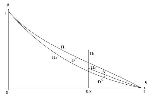
Fig. 2: Domains of global stability in coordinates $(\theta,\mu)$

Sometimes it will be more convenient for us to use the coordinates $(a,\theta)$ instead of $(\theta,\mu)$, we will preserve the same symbols for the domains and curves considered both in $(a,\theta)$ and $(\theta,\mu)$.

Let us end this section indicating several useful estimations which will be of great importance for the proof of our main result.

Lemma 12.

We have $\alpha(a,\theta)>0$, $\beta(a,\theta)>0$, and $a\alpha(a,\theta)/(1-a\beta(a,\theta))>-1$ for all $(a,\theta)\in\mathcal{D}$. Next, if $(a,\theta)\in\mathcal{S},$ then $\gamma(a,\theta)<1.$

The proof of the lemma is given in Section 6 (Lemmas 21, 22, 23).

4.2 One-dimensional map $\mathbf{F:I\to}\mathbb{R}$

Throughout this subsection, we will suppose that $(a,\theta)\in\mathcal{D}$. Therefore $a(\theta-1)/\theta-1>0$ so that the interval $I=(-1,a(\theta-1)/\theta-1)$ is not empty. Furthermore, $t_{1}=t_{1}(z)=-\ln(1-z/r(z))\in[-h,0]$ for every $z\in I\setminus\{0\}$. Consider now the map $F:I\to\mathbb{R}$ defined in the following way:

$$F(z)=\left\{\begin{array}[]{lll}0&{\rm if}\ z=0;\\ \min\limits_{t\in[0,h]}y(t,z)&{\rm if}\ z\in I\ {\rm and}\ z>0;\\ \max\limits_{t\in[0,h]}y(t,z)&{\rm if}\ z\in(-1,0),\end{array}\right.$$

where $y(t,z)$ is the solution of the initial value problem $y(s,z)=z,\ s\in[t_{1}(z)-h,t_{1}(z)],\ z\in I$ for

$$y^{\prime}(t)=-y(t)+r(y(t-h)).$$ (19)

Observe that $y(0,z)=0$ for all $z\in I$ since $y(t,z)=r(z)(1-\exp{(-t)})$ for all $t\in[t_{1}(z),t_{1}(z)+h]$. The following lemma explains why we have introduced such $F$ (moreover, condition (13) says precisely that $F^{\prime}(0)>-1$, see Section 6.2):

Lemma 13.

Let $x(t)$ be a solution of (14) and set $M=\limsup_{t\to\infty}x(t),$ $m=\liminf_{t\to\infty}x(t)$. If $m,M\in I$, then $m\geq F(M)$ and $M\leq F(m)$.

Proof.

Consider two sequences of extremal values $m_{j}=x(s_{j})\to m$, $M_{j}=x(t_{j})\to M$ such that $s_{j}\to+\infty,t_{j}\to+\infty$ as $j\to\infty$. Let $\varepsilon>0$ be such that $(m-\varepsilon,M+\varepsilon)\subset I$. Then $m_{j}\geq m-\varepsilon$ and $M_{j}\leq M+\varepsilon$ for big $j$. We will prove that $m\geq F(M)$, the case $M\leq F(m)$ being completely analogous.

By Lemma 10, we can find $\tau_{j}\in[s_{j}-h,s_{j}]$ such that $x(\tau_{j})=0$ while $x(t)<0$ for $t\in(\tau_{j},s_{j}]$. Next, $v_{j}=\tau_{j}+t_{1}(M+\varepsilon)\geq\tau_{j}-h$ because of $M+\varepsilon\in I$. Thus the solution $y(t)$ of Eq. (19) with initial condition $y(s)=M+\varepsilon,\ s\in[v_{j}-h,v_{j}]$, satisfies $y(\tau_{j})=0$ while $M+\varepsilon\equiv y(t)\geq x(t)$ for all $t\in[v_{j}-h,v_{j}]$. Furthermore, for all $s\in[v_{j},\tau_{j}],$ we have $\mathcal{M}(x_{s})\leq M+\varepsilon$ so that, by (15), $f(s,x_{s})\geq r(\mathcal{M}(x_{s}))\geq r(M+\varepsilon),$ and

$$y(t)-x(t)=\int_{\tau_{j}}^{t}e^{-(t-s)}[r(M+\varepsilon)-f(s,x_{s})]ds\geq 0,\ t\in[v_{j},\tau_{j}],$$

proving that $y(t)\geq x(t)$ for all $t\in[\tau_{j}-h,\tau_{j}]$. Now, for $t\in(\tau_{j},s_{j}],$

$$y(t)-x(t)=\int_{\tau_{j}}^{t}\exp\{-(t-s)\}(r(y(s-h))-f(s,x_{s}))ds\leq 0,$$ (20)

since $f(s,x_{s})\geq r(\mathcal{M}(x_{s}))\geq r(\mathcal{M}(y_{s}))=r(y(s-h))$. Hence, by (20), $m_{j}=x(s_{j})\geq y(s_{j})\geq F(M+\varepsilon)$ which proves that $m\geq F(M)$. ∎

To study the properties of $F$, we use its more explicit form given below:

Lemma 14.

Set $r^{-1}(u)=u/(a-u)$. For $z\in I$, $(F(z)-r(z))z\geq 0$ and

$$\theta=\int\limits_{r(z)}^{F(z)}\frac{du}{r^{-1}(u)-r(z)}.$$ (21)

Proof.

Let us consider $z>0$, the case $z<0$ being similar. Consider the solution $y(t,z)$ of Eq. (19), recall that $y(t,z)=z$ for $t\in[t_{1}-h,t_{1}],$ where $t_{1}=-\ln(1-z/r(z))\in[-h,0]$. Next, $y(t,z)=r(z)(1-\exp{(-t)}),\,t\in[t_{1},t_{1}+h]$ so that $y(0,z)=0$ and $y^{\prime}(h,z)=-y(h,z)$. Therefore $F(z)=y(t_{*},z)$ at some point $t_{*}\in(t_{1}+h,h)$ where also $y^{\prime}(t_{*},z)=0$.

Since $t_{*}\in[t_{1}+h,h]$, by the variation of constants formula we have

$$y(t_{*},z)=F(z)=e^{-(t_{*}-h)}\left[y(t_{1}+h,z)e^{t_{1}}+\int\limits_{t_{1}}^{t_{*}-h}e^{v}r(y(v,z))dv\right].$$ (22)

On the other hand, $y^{\prime}(t_{*},z)=0=-y(t_{*},z)+r(y(t_{*}-h,z))$, so that $F(z)=y(t_{*},z)=r(y(t_{*}-h,z))\geq r(z)$ and $r^{-1}(F(z))=y(t_{*}-h,z)=r(z)[1-\exp\{-(t_{*}-h)\}].$ Thus

$$t_{*}-h=\ln(r(z)/[r(z)-r^{-1}(F(z))]).$$

Let now $y(v,z)=w$ (so that $\exp(v)=r(z)/(r(z)-w)$), then

$$\int\limits_{t_{1}}^{t_{*}-h}e^{v}r(y(v,z))dv=\int\limits_{z}^{r^{-1}(F(z))}r(w)d\frac{r(z)}{r(z)-w}=$$

$$=r(z)\left[\frac{r(z)}{z-r(z)}-\frac{F(z)}{r^{-1}(F(z))-r(z)}+\int\limits_{z}^{r^{-1}(F(z))}\frac{dr(w)}{w-r(z)}\right].$$

Putting now the last expression and the values of $t_{1}$, $t_{*}-h$ in (22), we get (21). ∎

Finally, we state an important technical lemma whose proof can be found in Appendix, Lemmas 25, 26.

Lemma 15.

Assume that $(a,\theta)\in\mathcal{D}.$ Then $F(z)<\mathcal{R}(r(z))$ if $z\in((a\beta-1)^{-1},0),$ and $F(z)>\mathcal{R}(r(z))$ if $z\in(0,a(\theta-1)/\theta-1),$ where $\mathcal{R}$ is defined in Subsection 4.1.

We will also consider $\mathcal{F}:(a_{*},+\infty)\to\mathbb{R}$ defined by $\mathcal{F}(x)=F(x/(a-x))$. It can be easily seen that $\mathcal{F}(r(z))=F(z)$ for all $z\in I$.

4.3 One-dimensional map $\mathbf{F_{1}:[0,+\infty)\to}(a,0]$

By definition, for $z\geq 0,$ $F_{1}(z)=\min_{t\in[0,h]}y(t)$, where $y(t,z)$ satisfies (19) and has the initial value $y(s,z)=(1-e^{-s})r(z),\ s\in[-h,0]$. We will need the following

Lemma 16.

Let $x(t)$ be a solution of (14) and set $M=\limsup_{t\to\infty}x(t),$ $m=\liminf_{t\to\infty}x(t)$. If $(a,\theta)\in\mathcal{D}$, then $m\geq F_{1}(M).$

Proof.

Take $\varepsilon,s_{j},t_{j},m_{j},M_{j},\tau_{j}$ as in the first two paragraphs of the proof of Lemma 13. Then, for $t\in[\tau_{j}-h,\tau_{j}],$ we have

$$x(t)=\int_{\tau_{j}}^{t}e^{-(t-u)}f(u,x_{u})du\leq\int_{\tau_{j}}^{t}e^{-(t-u)}r(M+\varepsilon)du=y(t-\tau_{j},M+\varepsilon).$$

Thus, if $u\in[s_{j}-h,s_{j}]$, then $\mathcal{M}(x_{u}(s))\leq\mathcal{M}(y_{u}(s,M+\varepsilon))$ so that

$$f(u,x_{u})\geq r(\mathcal{M}(y_{u}(s,M+\varepsilon)))=r(r(M)(1-e^{-(u-h-\tau_{j})})).$$

This implies that

$$m_{j} = x(s_{j})\geq\int_{\tau_{j}}^{s_{j}}e^{-(s_{j}-u)}r(r(M)(1-e^{-(u-h-\tau_{j})}))du$$

$$= \int_{\tau_{j}}^{s_{j}}e^{-(s_{j}-u)}r(y(u-h,M+\varepsilon))du=y(s_{j}-\tau_{j},M+\varepsilon)\geq F_{1}(M+\varepsilon).$$

Since $\varepsilon>0$ and $m_{j}\to m$ are arbitrary, the lemma is proved. ∎

Lemma 17.

Set $r_{1}(z)=r(r(z)(1-e^{h}))$. For $z>0$ we have that $F_{1}(z)>a$ and

$$\frac{r_{1}(z)\theta}{r(z)}=\int_{r_{1}(z)}^{F_{1}(z)}\frac{du}{r^{-1}(u)-r(z)}.$$ (23)

Proof.

Take $t_{*}\in(0,h)$ such that

$$F_{1}(z)=y(t_{*},z)=\int_{0}^{t_{*}}e^{-(t_{*}-u)}r(r(z)(1-e^{-(u-h)}))du.$$ (24)

Since $y^{\prime}(h)>0$, we have that $y^{\prime}(t_{*})=0$ and therefore $F_{1}(z)=y(t_{*})=-y^{\prime}(t_{*})+r(y(t_{*}-h))=r(y(t_{*}-h))>a.$ This implies that $r^{-1}(F_{1}(z))=y(t_{*}-h)=r(z)(1-\exp\{-(t_{*}-h)\}),$ from where

$$t_{*}-h=\ln(r(z)/[r(z)-r^{-1}(F_{1}(z))]).$$ (25)

Now, using (25) and setting $\xi=r(z)(1-e^{-(u-h)})$ in (24), we obtain

$$F_{1}(z) = -(r(z)-r^{-1}(F_{1}(z)))\int_{r(z)(1-e^{h})}^{r^{-1}(F_{1}(z))}r(\xi)d\frac{1}{\xi-r(z)}$$

$$= -(r(z)-r^{-1}(F_{1}(z)))\Biggl{(}\frac{r(\xi)}{\xi-r(z)}\Biggl{|}_{r(z)(1-e^{h})}^{r^{-1}(F_{1}(z))}+\int_{r(z)(1-e^{h})}^{r^{-1}(F_{1}(z))}\frac{dr(\xi)}{\xi-r(z)}\Biggl{)}.$$

Simplifying this relation, we obtain (23). ∎

We conclude this section by stating two lemmas which compare $F_{1}$ and the associated function $\mathcal{F}_{1}(r)\stackrel{{\scriptstyle def}}{{=}}F_{1}(r/(a-r))$ with rational functions. The proofs of these statements are based on rather careful estimations of identity (23) and are given in Appendix, Lemmas 27, 30, 31 (it should be noted that $\mathcal{R}$ approximates extremely well $\mathcal{F}_{1}$ so that a very meticulous analysis of (23) is needed).

Lemma 18.

If $(a,\theta)\in\mathcal{D}^{*}$ and $z\geq a(\theta-1)/\theta-1$ then $F_{1}(z)>\mathcal{R}(r(z)).$

Lemma 19.

If $(a,\theta)\in\mathcal{S}$ and $z>0$, then

$$\mathcal{F}_{1}(r(z))>\frac{1+\ln\theta-\theta}{2+\ln\theta-\theta}\frac{ar(z)}{1+r(z)\frac{1+\ln\theta-\theta}{1-\theta}}=\mathcal{R}_{2}(r(z)).$$ (26)

Furthermore, $\mathcal{R}_{2}(a)>-1$ and $r(\mathcal{R}_{2}(a))<1/\beta.$

4.4 Proof of Theorem 1

Let $x:[\alpha-h,\infty)\to\mathbb{R}$ be a solution of Eq. (14) and set $M=\limsup_{t\to\infty}x(t),\ m=\liminf_{t\to\infty}x(t)$. We will reach a contradiction if we assume that $m<0<M$ (note that the cases $M\leq 0$ and $m\geq 0$ were already considered in Lemma 9).

First suppose that $(a,\theta)\in\mathcal{S}$. By Lemmas 16 and 19, we obtain that

$$m\ \geq\ F_{1}(M)=\mathcal{F}_{1}(r(M))\ >\ \mathcal{R}_{2}(r(M))>-1.$$ (27)

Take now an arbitrary $z\geq 0$. Since $r(z)\in(a,0]$ and $\mathcal{R}_{2}(z)$ is increasing on $(a,0]$, we get $r(\mathcal{R}_{2}(r(z)))<1/\beta$ due to Lemma 19. Therefore, the rational function $\lambda\stackrel{{\scriptstyle def}}{{=}}\mathcal{R}\circ r\circ\mathcal{R}_{2}\circ r:[0,\infty)\to[0,\infty)$ is well defined. By Lemmas 13 and 15, we obtain

$$M\leq\mathcal{F}(r(m))<\mathcal{R}(r(\mathcal{R}_{2}(r(M))))=\lambda(M).$$

On the other hand, due to the inequality $\lambda^{\prime}(0)=\gamma(a,\theta)<1$ (see Lemma 12), we obtain that $\lambda(z)<z$ for all $z>0$, a contradiction.

Let now $(a,\theta)\in\mathcal{D}^{*}$ and define the rational function $R:[0,+\infty)\to(-\infty,0]$ as $R=\mathcal{R}\circ r$. We note that (13) implies $R^{\prime}(0)=a\alpha(a,\theta)\in(-1,0)$. Next,

$$m>R(M)>\mathcal{R}(a)>-1.$$ (28)

Indeed, if $M\leq a(\theta-1)/\theta-1,$ then Lemmas 13 and 15 imply that $m\geq F(M)>\mathcal{R}(r(M))=R(M)$. If $M\geq a(\theta-1)/\theta-1,$ then Lemmas 16 and 18 give that $m\geq F_{1}(M)>\mathcal{R}(r(M))=R(M).$ The last inequality in (28) follows from Lemma 12. Finally, applying Lemmas 13 and 15, and using (28) and the inequality $R\circ R(x)<x,\ x>0,$ which holds since $(R\circ R)^{\prime}(0)=(R^{\prime}(0))^{2}<1$, we obtain that

$$M\leq F(m)<\mathcal{R}(r(m))<\mathcal{R}(r(R(M)))=R(R(M))<M,$$

a contradiction.

To prove the second part of Theorem 1 take $a<0$ and $h>0$ such that (13) is not satisfied. Then, by Theorem 2.9 from [6] there is a continuous functional $f$ satisfying (5) and such that the equilibrium $x(t)=0$ in (14) is not locally asymptotically stable.

5 Some estimations of the global attractor for (11)

To complete the proof of Theorem 2, we need to estimate the bounds of the global attractor to (11). We start by stating a result from [3]

Lemma 20.

[3] Let $q>1$. Then there exist finite positive limits

$$M=\limsup_{t\to\infty}x(t)\,,\,m=\liminf_{t\to\infty}x(t)$$

for every nonnegative solution $x(t)\not\equiv 0$ of (11). Moreover, $[m,M]\subseteq g([m,M])$ and $[m,M]\subseteq g_{1}([m,M]),$ where $g_{1}=\theta\ln q+(1-\theta)g,\ \theta=\exp(-\tau).$

Since the global stability of Eq. (11) for $\ln q\in(0,2]$ was already proved in [3], we can suppose that $\ln q>2$. In this case the minimal root $x_{1}$ of equation $g(x_{1})=\ln q\$ belongs to the interval $(0,1)$. Note that $x=1<\ln q$ is the point of absolute maximum for $g$ and $g_{1}=(1-\theta)g+\theta\ln q,$ so that $g(1)>\ln q$ and $g_{1}(1)>\ln q$. We will use the information about the values of $g$ and $g_{1}$ at $x_{1}<1<\ln q$ in the subsequent analysis.

Now, let us consider an arbitrary solution $x(t)$ of (11) and its bounds $m,M$ defined in Lemma 20. It is clear that if we prove the existence of $m_{*}=m_{*}(q)$ such that $m\geq m_{*}(q)>x_{1}$ and $m_{*}(q)$ does not depend on $x(t)$, then the change of variables $y=x-\ln q$ transforms Eq. (11) into an equation satisfying (W) within the domain of attraction, and therefore Theorem 1 can be applied.

Since $[m,M]\subseteq g([m,M])$, we obtain immediately that either $m=M=\ln q$ or $m<\ln q<M.$ In the first case the theorem is proved, so we will consider the second possibility. Next, since $z<g(z)$ for $z\in(0,\ln q)$, we have that $g(m)>m$ and

$$[m,M]\subseteq g([m,M])\subseteq[\min\{g(m),g(M)\},g(1)]=[g(M),g(1)].$$

Hence, $[m,M]\subseteq g([g(M),g(1)])\subseteq[\min\{g^{2}(1),g^{2}(M)\},g(1)]$. On the other hand, since $g(M)<\ln q$ we get analogously that $g^{2}(M)>g(M)$. Next, since $g$ is decreasing on $[1,+\infty)$ and $g(1)\geq M$ we find that $g^{2}(1)\leq g(M)$. Thus $g^{2}(1)\leq g(M)<g^{2}(M)$ so that $\min\{g^{2}(1),g^{2}(M)\}=g^{2}(1)$ and $[m,M]\subseteq[g^{2}(1),g(1)]$. Therefore $m\geq g(g(1))$. Since the inequality $m\geq g_{1}(g_{1}(1))$ can be proved analogously, the proof of theorem will be completed if we establish that $m_{*}(q)=\max\{g^{2}(1),g_{1}^{2}(1)\}>x_{1}$. We have

(i) $g^{2}(1)>x_{1}$ for all $\ln q\in[2,2.833157].$ This is an obvious fact if $g^{2}(1)\geq 1$, so that we only need to consider the case $x_{1},g^{2}(1)\in(0,1)$. Since $g$ is increasing on $(0,1)$, the inequality $g^{2}(1)>x_{1}$ is equivalent to $g^{3}(1)>g(x_{1})=\ln q$ in this case. Finally, a direct computation shows that

$$g^{3}(1)-\ln q=q^{3}e^{-1-q/e}\exp(-q^{2}e^{-1-q/e})-\ln q>0$$

whenever $\ln q\in[2,2.833157].$

(ii) $g_{1}^{2}(1)>x_{1}$ for all $\ln q>2.5$. First, let us note that $x_{1}\leq\ln q+y_{1},$ where

$$y_{1}=\left(2-\ln q-\sqrt{(\ln q)^{2}+4\ln q-4}\right)/2$$

is the negative root of $\tilde{g}(y)=(y+\ln q)(1-y+y^{2}/2)-\ln q$. Indeed, with $x=y+\ln q$ and $y\in(y_{1},0)$, we have that $g(x)-\ln q=qxe^{-x}-\ln q=(y+\ln q)e^{-y}-\ln q\geq\tilde{g}(y)>0.$

Since $g_{1}^{2}(1)\geq g_{1}(+\infty)=\theta\ln q,$ to finish the proof of (ii), it suffices to show that $\theta\ln q\geq\ln q+y_{1}.$ Taking into account (10) and using the inequality $\ln(1+x)\geq x/(1+x)$, we obtain that

$$(\theta-1)\ln q-y_{1} = (\theta-1)(1+c)-y_{1}\geq(1+c)(-1+c\ln((c^{2}+c)/(c^{2}+1))-y_{1}$$

$$\geq -2-\frac{2-\ln q-\sqrt{(\ln q)^{2}+4\ln q-4}}{2}\geq 0,\quad{\rm for}\quad\ln q\geq 5/2.$$

6 Appendix

6.1 Preliminary estimations

 

Lemma 21.

For all $(a,\theta)\in\mathcal{D}$, we have that $\alpha(a,\theta)>0,\ \beta(a,\theta)>0$, and

$$T(a,\theta)\stackrel{{\scriptstyle def}}{{=}}\ (a^{2}-a)\beta(a,\theta)(1-\theta)+\alpha(a,\theta)-(1-\theta)\geq 0.$$

Proof.

Since $a(\theta-1)>1$ for all $(a,\theta)\in\mathcal{D}$ and

$$\begin{array}[]{ll}1+x<\exp(x)<1+x+x^{2}/2&\;{\rm for}\ x<0,\\ \vskip 3.0pt plus 1.0pt minus 1.0pt\cr\exp(x)>1+x+x^{2}/2+x^{3}/6&\;{\rm for}\ x>0,\end{array}$$ (29)

we have $\alpha(a,\theta)=(1-a)\exp(\theta/a)+a>(1-a)(1+\theta/a)+a=1-\theta+\theta/a>0.$ Analogously, $\beta(a,\theta)>0$ for all $(a,\theta)\in\mathcal{D}$ because of the following chain of relations

$$- a\alpha(a,\theta)\beta(a,\theta)e^{-\theta/a}=a^{2}e^{-\theta/a}-(1-a)^{2}e^{\theta/a}+(1-2a+2\theta(a-1))$$

$$\geq a^{2}(1-\frac{\theta}{a}+\frac{\theta^{2}}{2a^{2}}-\frac{\theta^{3}}{6a^{3}})-(1-a)^{2}(1+\frac{\theta}{a}+\frac{\theta^{2}}{2a^{2}})+(1-2a+2\theta(a-1))$$

$$= \frac{\theta}{6a^{2}}(-3\theta-a(\theta^{2}-6\theta+6))>\frac{\theta(2\theta a-2a-\theta)}{2a^{2}}>0.$$

To prove that $T(a,\theta)\geq 0$ for all $(a,\theta)\in\mathcal{D}$, we replace $\alpha,\beta$ with their values in $\alpha T$:

$$\begin{array}[]{ll}\quad\alpha(a,\theta)T(a,\theta)=&\!\!\!a(2a-a^{2}-a\theta+a^{2}\theta-1+\theta)\\[5.69054pt] &\!\!\!+2\theta(a-1)(-2a+a\theta+1-\theta)\lambda-(1-a)^{2}(-a+a\theta-\theta)\lambda^{2}.\end{array}$$ (30)

It should be noticed that $-a+a\theta-\theta=a(\theta-1)-\theta>1-\theta>0$. Similarly, $2\theta(a-1)(-2a+a\theta+1-\theta)<0$ so that $T(a,\theta)\geq 0$ if

$$\theta(-a+a\theta-\theta)(4a^{4})^{-1}[-\theta(-\theta+a\theta-2a)^{2}+4(\theta-1)a^{3}]>0,$$

where the last expression was obtained from (30) by replacing $\lambda=\exp(\theta/a)$ by $1+\theta/a+\theta^{2}/2a^{2}>\exp(\theta/a)$. Taking into account that $a(\theta-1)>1$ and $\theta<1$ for $(a,\theta)\in\mathcal{D}$, we end the proof of this lemma by noting that $4(\theta-1)a^{3}-\theta(\theta-a\theta+2a)^{2}\geq 4a^{2}-(\theta-a\theta+2a)^{2}=(-4a-\theta+a\theta)\theta(1-a)>0.$ ∎

Lemma 22.

For all $(a,\theta)\in\mathcal{D}$ one has

$$\frac{a\alpha(a,\theta)}{1-a\beta(a,\theta)}>-1.$$ (31)

Proof.

It follows directly from the definitions of $\alpha(a,\theta)$ and $\mathcal{D}$ that $a\alpha(a,\theta)>-1$ for all $(a,\theta)\in\mathcal{D}$. Now, (31) follows from the fact that $a\beta(a,\theta)<0$ if $(a,\theta)\in\mathcal{D}$. ∎

Lemma 23.

If $(a,\theta)\in\mathcal{S},$ then $\gamma(a,\theta)<1.$

Proof.

Notice that $(a,\theta)\in\mathcal{S}$ implies that $\theta\in[0.8,1)$ and $\theta>\Pi_{3}(-1/a)$ (or, equivalently, $a>\pi_{3}(\theta)\stackrel{{\scriptstyle def}}{{=}}-1/\Pi_{3}^{-1}(\theta)=(108+25\theta)(95\theta-95)^{-1}$). Here $\Pi_{3}^{-1}$ is the inverse function of $\Pi_{3}$. Next we prove the inequality

$$\frac{1-\theta+\ln\theta}{2-\theta+\ln\theta}+\frac{(\theta-1)^{2}(2-\theta)}{2}>0,\quad\theta\in[0.8,1),$$ (32)

which is equivalent to the relation

$$\Xi(q)\stackrel{{\scriptstyle def}}{{=}}q(q-2)(q^{2}+1)+(2+q^{2}-q^{3})\ln(q+1)>0,\quad q\in[-0.2,0),$$

with $\theta=q+1$ (note that $1-q+\ln(q+1)>0$ for $q\in[-0.2,0)$). To do that, we will need the following approximation of $\ln(1+q)$ when $q\in[-0.2,0)$:

$$\ln(1+q)>q-0.5q^{2}+0.4q^{3},\ \ q\in[-0.2,0).$$ (33)

(Indeed, function $y(x)=\ln(1+x)-(x-0.5x^{2}+0.4x^{3})$ has exactly one critical point $x=-1/6$ on $[-0.2,0)$, and $y(-0.2)=0.00005644\dots>0$, $y(0)=0$). Inequality (33) implies that $\Xi(q)\geq-0.1q^{3}(5q+2-9q^{2}+4q^{3}).$ Now, since $(5q+2-9q^{2}+4q^{3})>0$ for all $q\in[-0.2,0)$, we have that $\Xi(q)>0$ and thus (32) is proved.

Next, due to (29) and (32),

$$\gamma(a,\theta)\leq a^{3}(1-\theta+\frac{\theta}{a}-\frac{\theta^{2}}{2a}+\frac{\theta^{2}}{2a^{2}})\frac{(\theta-1)^{2}(\theta-2)}{2}=w(a,\theta),$$

so that $\gamma(\pi_{3}(\theta),\theta))\leq w(\pi_{3}(\theta),\theta)).$ Now, $w(\pi_{3}(\theta),\theta))$ is a fifth degree polynomial and an elementary analysis shows that $w(\pi_{3}(\theta),\theta))<1$ for all $\theta\in[0.8,1).$ Since

$$\partial w(a,\theta)/\partial a=0.25(2-\theta)(\theta-1)^{2}[a(\theta-1)(2a+2\theta)+a(4a(\theta-1)-2\theta)]<0,$$

we conclude that $\gamma(a,\theta)\leq w(a,\theta)<1$ for $a>\pi_{3}(\theta).$ ∎

Lemma 24.

Let $(a,\theta)\in\mathcal{D}$ and $r>-1/4$. Set $\mathcal{J}(r)=\mathcal{I}(N(r))$, where $\mathcal{I}(N)=N\coth(\nu N/2),\ \nu=-\theta/a,\ N(r)=\sqrt{1+4r}.$ Then $\mathcal{J}^{\prime}(0)>0$ and

$$\mathcal{J}(r)\leq\mathcal{J}(0)+\mathcal{J}^{\prime}(0)r=\frac{1+\lambda}{1-\lambda}+\Biggl{(}2\frac{1+\lambda}{1-\lambda}+\frac{4\theta\lambda}{a(1-\lambda)^{2}}\Biggl{)}r.$$ (34)

Proof.

Set $k(N)=e^{2\nu N}-2\nu Ne^{\nu N}-1>0$; then $k(0)=0$ and $k^{\prime}(N)=2\nu e^{\nu N}[e^{\nu N}-1-\nu N]>0$ for all $N>0$. Hence $\mathcal{I}\,^{\prime}(N)=k(N)/(e^{\nu N}-1)^{2}>0$ and $\mathcal{J}^{\prime}(0)=\mathcal{I}\,^{\prime}(1)N^{\prime}(0)>0.$

Next, since $dN/dr=2(1+4r)^{-1/2}=2/N,\quad d^{2}N/dr^{2}=-4/N^{3},$ we obtain that

$$\mathcal{J}^{\prime\prime}(r) = \frac{\partial^{2}\mathcal{I}(N(r))}{\partial r^{2}}=\frac{\partial^{2}\mathcal{I}(N)}{\partial N^{2}}\Biggl{(}\frac{\partial N(r)}{\partial r}\Biggl{)}^{2}+\frac{\partial\mathcal{I}(N)}{\partial N}\Biggl{(}\frac{\partial^{2}N(r)}{\partial r^{2}}\Biggl{)}$$

$$= \frac{4[-e^{3\nu N}+e^{2\nu N}(2\nu^{2}N^{2}-2\nu N+1)+e^{\nu N}(2\nu^{2}N^{2}+2\nu N+1)-1]}{N^{3}(e^{\nu N}-1)^{3}}$$

$$= \frac{\sum_{j=0}^{+\infty}p_{j}(\nu N)^{j}}{N^{3}(e^{\nu N}-1)^{3}}<0,\quad{\rm since\ }(\nu N)>0,\ p_{j}=0,\ j=0,\dots,5,{\rm\ and}$$

$$p_{j}=\frac{4}{(j-2)!}\Bigl{(}\frac{-3^{j}+2^{j}+1}{j(j-1)}+\frac{-2^{j}+2}{j-1}+2^{j-1}+2\Bigl{)}<0,\ j\geq 6.$$

Thus $\mathcal{J}(r)\leq\mathcal{J}(0)+\mathcal{J}^{\prime}(0)r$ and (34) is proved. ∎

6.2 Properties of function $\mathbf{F}$

To study the properties of functions $F:I\to\mathbb{R}$ and $\mathcal{F}:J=(a_{*},+\infty)\to\mathbb{R},$ defined in subsection 4.2, it will be more convenient to use the integral representation (21) instead of the original definition of $F$. It should be noted that conditions $xF(x)<0,\ (F(x)-r(x))x>0,\ x\in I\setminus\{0\}$ define $F$ in a unique way: moreover $F$ and $\mathcal{F}$ are continuous and smooth at $0$ with $\mathcal{F}^{\prime}(0)=\alpha(a,\theta)$, $\mathcal{F}^{\prime\prime}(0)=2\alpha(a,\theta)\beta(a,\theta)$. We have taken into consideration these facts to define the rational functions $R$ and $\mathcal{R}$ (see Subsection 4.2); however, since we do not use anywhere these characteristics of $F$, their proof is omitted here.

Lemma 25.

Assume that $r\in[a_{*},0]$. Then

$$\mathcal{F}(r)>\alpha\,r/(1-\beta r)=\mathcal{R}(r).$$ (35)

Proof.

1. First, suppose that $4r+1>0$ and $r\not=0$. Since $0>\mathcal{F}(r)>r$, we have, for every $z\in[r,\mathcal{F}(r)]$ and $a<0$,

$$r^{-1}(z)=z/(a-z)=(z/a)(1+(z/a)+(z/a)^{2}+\cdots)>(z/a)+(z/a)^{2}.$$ (36)

Hence

$$\theta=\int_{r}^{\mathcal{F}(r)}\frac{dz}{z(a-z)^{-1}-r}<\int\limits_{r}^{\mathcal{F}(r)}\frac{dz}{\frac{z}{a}+(\frac{z}{a})^{2}-r}=a\int\limits_{r/a}^{\mathcal{F}(r)/a}\frac{du}{u+u^{2}-r}.$$ (37)

Now, since for $r<0$ the roots $\alpha_{1}=(-1-\sqrt{1+4r})/2,\quad\alpha_{2}=(-1+\sqrt{1+4r})/2$ of the equation $u^{2}+u-r=0$ are negative, we obtain

$$a\int\limits_{r/a}^{\mathcal{F}(r)/a}\frac{du}{u+u^{2}-r}=-\frac{a}{\sqrt{1+4r}}\ln\Bigl{(}\frac{\mathcal{F}(r)-a\alpha_{1}}{\mathcal{F}(r)-a\alpha_{2}}\ \frac{r-a\alpha_{2}}{r-a\alpha_{1}}\Bigl{)}>\theta.$$ (38)

The last inequality implies that

$$\frac{\mathcal{F}(r)-a\alpha_{1}}{\mathcal{F}(r)-a\alpha_{2}}\ \frac{r-a\alpha_{2}}{r-a\alpha_{1}}>\exp(\frac{\theta\sqrt{1+4r}}{-a})\stackrel{{\scriptstyle def}}{{=}}\omega(r)\geq 1.$$ (39)

Taking into account that $\mathcal{F}(r)-a\alpha_{2}<0$ and $r-a\alpha_{1}<0$, and replacing $\alpha_{1},\alpha_{2}$ in (39) by their values, we obtain

$$\mathcal{F}(r)>\frac{r(2a^{2}-a+a\frac{\omega(r)+1}{\omega(r)-1}\sqrt{1+4r})}{2r+a+a\frac{\omega(r)+1}{\omega(r)-1}\sqrt{1+4r}}.$$

Next, since $\mathcal{J}(r)=\frac{\omega(r)+1}{\omega(r)-1}\sqrt{1+4r}$, we can apply Lemma 24 to see that

$$\begin{array}[]{ll}\mathcal{F}(r)&\!\!\!>\displaystyle\frac{r(2a-1+\mathcal{J}(r))}{2r/a+1+\mathcal{J}(r)}\ \geq\ \displaystyle\frac{r(2a-1+\mathcal{J}(0)+\mathcal{J}^{\prime}(0)r)}{2r/a+1+\mathcal{J}(0)+\mathcal{J}^{\prime}(0)r}\\ \vskip 6.0pt plus 2.0pt minus 2.0pt\cr&\!\!\!=\displaystyle\frac{r(\lambda+a(1-\lambda))+\frac{1}{2}\mathcal{J}^{\prime}(0)(1-\lambda)r^{2}}{1+(\frac{1-\lambda}{a}+\frac{1}{2}\mathcal{J}^{\prime}(0)(1-\lambda))r}\stackrel{{\scriptstyle def}}{{=}}\mathcal{L}(r).\end{array}$$

Now, $\mathcal{L}(r)=(a_{1}r+a_{2}r^{2})/(1+a_{3}r)$, with $a_{1}>0,a_{2}>0$. Moreover, since $0<\mathcal{J}(r)\leq\mathcal{J}(0)+\mathcal{J}^{\prime}(0)r,$ all denominators in (6.2) are positive so that $1+a_{3}r>0$. Next,

$$\qquad a_{1}a_{3}-a_{2}=(\lambda+a(1-\lambda))\Biggl{(}\frac{1-\lambda}{a}+\frac{1}{2}\mathcal{J}^{\prime}(0)(1-\lambda)\Biggl{)}-\frac{1}{2}\mathcal{J}^{\prime}(0)(1-\lambda)\leq 0.$$ (40)

Indeed, the last inequality is equivalent to the obvious relation

$$\frac{\lambda+a(1-\lambda)}{a}<0\leq\frac{1}{2}(1-\lambda)(1-a)\mathcal{J}^{\prime}(0)$$

(notice that $\alpha=\lambda+a(1-\lambda)>0,$ while, by Lemma 24, $\mathcal{J}^{\prime}(0)>0$).

Finally, since the inequality $(a_{1}r+a_{2}r^{2})(1+a_{3}r)^{-1}\geq a_{1}r(1+(a_{3}-a_{2}/a_{1})r)^{-1}$ holds for $r<0,\ a_{1}>0,\ a_{2}>0,\ 1+a_{3}r>0,\ a_{1}a_{3}\leq a_{2}$, we obtain

$$\mathcal{F}(r)>\frac{a_{1}r}{1+(a_{3}-\frac{a_{2}}{a_{1}})r}=\frac{r(\lambda+a(1-\lambda))}{1+(\frac{1-\lambda}{a}+\mathcal{J}^{\prime}(0)\frac{1-\lambda}{2}-\frac{\mathcal{J}^{\prime}(0)(1-\lambda)}{2(\lambda+a(1-\lambda))})r}=\mathcal{R}(r).$$

Hence the statement of the lemma is proved for $r\in(-1/4,0)$. As an important consequence of the first part of proof, we get the following relation

$$\lim\limits_{r\to-1/4}\frac{r(2a^{2}-a+a\frac{\omega(r)+1}{\omega(r)-1}\sqrt{1+4r})}{2r+a+a\frac{\omega(r)+1}{\omega(r)-1}\sqrt{1+4r}}=\frac{a^{2}(1-\theta)+\theta a/2}{\theta(2a-1)-4a^{2}}\geq\mathcal{R}(-1/4),$$

which will be used in the next stage of proof.

2. The case $r=-1/4.$

From (37), evaluated at $r=-1/4$, we get $\theta<(-2a^{2})/(2\mathcal{F}(-1/4)+a)+(4a^{2})/(2a-1),$ so that

$$\mathcal{F}(-1/4)>\frac{a^{2}(1-\theta)+\theta a/2}{\theta(2a-1)-4a^{2}}\geq\mathcal{R}(-1/4).$$

3. Assume now that $4r+1<0.$ We have

$$\qquad\quad a\int\limits_{r/a}^{\mathcal{F}(r)/a}\frac{du}{u+u^{2}-r}=\frac{2a}{\sqrt{-4r-1}}\Biggl{(}\arctan\frac{2\mathcal{F}(r)+a}{a\sqrt{-4r-1}}-\arctan\frac{2r+a}{a\sqrt{-4r-1}}\Biggl{)}.$$ (41)

By (37) and (41), we obtain

$$2\mathcal{F}(r)+a>a\sqrt{-4r-1}\frac{\frac{2r+a}{a\sqrt{-4r-1}}+\tan\frac{\theta\sqrt{-4r-1}}{2a}}{1-\frac{2r+a}{a\sqrt{-4r-1}}\tan\frac{\theta\sqrt{-4r-1}}{2a}}.$$

Now, since $\tan x\leq x+x^{3}/3$ for $x\in(-\pi/2,0)$ and $a<0$, we obtain

$$\mathcal{F}(r)>r\frac{a^{2}(1-\theta)+\theta a/2+\theta^{3}(-r-\frac{1}{4})(\frac{1}{2a}-1)(3)^{-1}}{a^{2}-\theta(r+\frac{a}{2})-\theta^{3}(-r-\frac{1}{4})(\frac{a}{2}+r)(3a^{2})^{-1}}=G(r).$$ (42)

Therefore it will be sufficient to establish that $G(r)\geq\mathcal{R}(r)$ for $r<-1/4$. First, note that by the second part of the proof

$$G(-1/4)=\frac{a^{2}(1-\theta)+\theta a/2}{\theta(2a-1)-4a^{2}}\geq\mathcal{R}(-1/4).$$

Let us consider now the function $H(r)=G(r)-\mathcal{R}(r)$ for $r\leq 0.$ Since $G(r)=G_{1}(r)/G_{2}(r)$, where $G_{j}$ are polynomials in $r$ of second degree, $H(r)$ can be written as

$$H(r)=\frac{G_{1}(r)(1-\beta r)-\alpha rG_{2}(r)}{G_{2}(r)(1-\beta r)}=\frac{H_{1}(r)}{H_{2}(r)},$$ (43)

so that $H$ is a quotient of two polynomials of third degree with $H_{2}(r)>0$ for $r\leq 0.$ We get $\lim_{r\to-\infty}G(r)=a^{2}(1-1/(2a))>0,$ and therefore $H(-\infty)=\lim_{r\to-\infty}H(r)>0.$ Furthermore, $H(0)=0$ and

$$H^{\prime}(0)=\frac{1-\theta(1-\frac{1}{2a})+\frac{\theta^{3}}{12a^{2}}(1-\frac{1}{2a})}{1-\frac{\theta}{2a}+\frac{\theta^{3}}{24a^{3}}}-(a+e^{\frac{\theta}{a}}(1-a))=\frac{\sum_{k=5}^{+\infty}p_{k}\theta^{k}}{1-\frac{\theta}{2a}+\frac{\theta^{3}}{24a^{3}}}>0,$$

since the denominator of the last fraction is positive and $p_{2m+1}>0,\ p_{2m}<0,\ p_{2m+1}+p_{2m+2}>0$ for $m\geq 2$. Here we use the formula

$$p_{k}=\frac{a-1}{a^{k}k!}(1-\frac{k}{2}+\frac{k(k-1)(k-2)}{24}),\ k\geq 5.$$

Finally, since $H(-1/4)=G(-1/4)-\mathcal{R}(-1/4)\geq 0$, there exists at least one zero of $H(r)$ in the interval $[-1/4,0)$. $H_{1}(r)$ is a polynomial of third degree in $r$ and therefore it cannot have more than three zeros. Hence, since $H(-\infty)>0$ and $H(-1/4)\geq 0,$ we obtain that $H(r)\geq 0$ if $r<-1/4.$ ∎

Lemma 26.

If $(a,\theta)\in\mathcal{D}$, then $\mathcal{F}(r)<\mathcal{R}(r)$ for all $r\in(0,1/\beta)$.

Proof.

By definition of $\mathcal{F}$, we have that $z>0$ if $r>0$ and $z\in[\mathcal{F}(r),r]$. We begin the proof by assuming that $r\in(0,a^{2}-a).$ Since $z>0,a<0$, we find that $z(a-z)^{-1}<z/a+z^{2}/a^{2}$. Therefore, (37) holds under our present conditions. Now, since $r>0$, the roots of equation $u^{2}+u-r=0$ are $\alpha_{1}=(-1-\sqrt{1+4r})/2<0,\quad\alpha_{2}=(-1+\sqrt{1+4r})/2>0.$ Next, since $\mathcal{F}(r)-a\alpha_{1}<r-a\alpha_{1}<0$ for all $r\in(0,a^{2}-a)$, we obtain that the relations (38), (39) hold in the new situation and therefore

$$\mathcal{F}(r)<\frac{a^{2}\alpha_{1}\alpha_{2}(\omega(r)-1)+ar(\alpha_{1}-\omega(r)\alpha_{2})}{-a\alpha_{2}+r+\omega(r)(a\alpha_{1}-r)}=\frac{r(2a^{2}-a+a\frac{\omega(r)+1}{\omega(r)-1}\sqrt{1+4r})}{2r+a+a\frac{\omega(r)+1}{\omega(r)-1}\sqrt{1+4r}},$$

where the denominator is positive for every $r\in(0,a^{2}-a)$. Now, recall that $\mathcal{J}(r)=\frac{\omega(r)+1}{\omega(r)-1}\sqrt{1+4r}$ ; applying Lemma 24, we obtain $\mathcal{J}(r)\leq\mathcal{J}(0)+\mathcal{J}^{\prime}(0)r$. Next, since for all $r\in(0,a^{2}-a)$ we have that $2r/a+1+\mathcal{J}(r)=-2(a(\omega(r)-1))^{-1}(-a\alpha_{2}+r+\omega(r)(a\alpha_{1}-r))>0,$ and the function $p(x)=(r(2a-1+x))(2r/a+1+x)^{-1}$ is increasing in $x$, we get $\mathcal{F}(r)<\mathcal{L}(r)$ (compare with (6.2)). Now, $(a_{1}r+a_{2}r^{2})(1+a_{3}r)^{-1}\leq a_{1}r(1+(a_{3}-a_{2}/a_{1})r)^{-1}$ if $a_{1}a_{3}-a_{2}\leq 0,\ r>0,$ $\ a_{1}>0,\ a_{2}>0$ . Therefore, by (40), $\mathcal{L}(r)\leq\mathcal{R}(r)$.

Now we assume that $r\geq a^{2}-a.$ Taking into account that $z(a-z)^{-1}<0$ for $z>0,$ we obtain the inequality

$$\theta=\int_{r}^{\mathcal{F}(r)}\frac{dz}{z(a-z)^{-1}-r}<\int_{r}^{\mathcal{F}(r)}\frac{dz}{-r}=\frac{\mathcal{F}(r)-r}{-r},$$

so that $\mathcal{F}(r)<r(1-\theta)$. Finally, the inequality $r(1-\theta)\leq\mathcal{R}(r)=\alpha r/(1-\beta r)$ is equivalent to $r\geq(1-\theta-\alpha)/((1-\theta)\beta)$, which holds for all $r\geq a^{2}-a$ due to the relation $a^{2}-a\geq(1-\theta-\alpha)/((1-\theta)\beta)$, established in Lemma 21. ∎

6.3 Properties of function $\mathbf{F_{1}}$ in the domain $\mathcal{D}^{*}$

Suppose now that $(a,\theta)\in\mathcal{D}^{*}.$ We study some properties of function $F_{1}$ and the associated function $\mathcal{F}_{1}:(a,0)\to\mathbb{R}$ defined as $\mathcal{F}_{1}(r(z))=F_{1}(z),$ which, by Lemma 17, satisfies

$$\frac{r_{1}(r)\theta}{r}=\int\limits_{r_{1}(r)}^{\mathcal{F}_{1}(r)}\frac{dz}{r^{-1}(z)-r}\,,\,\mbox{ where }r_{1}(r)=\frac{ar(\theta-1)}{\theta+r(\theta-1)}.$$

Lemma 27.

Assume that $(a,\theta)\in\mathcal{D}^{*}$ and that the inequalities $a<r\leq a_{*}=a+\theta/(1-\theta)$ hold. Then $\mathcal{F}_{1}(r)>\mathcal{R}(r).$

Proof.

Since $r_{1}(r)<\mathcal{F}_{1}(r)<0$ and $a_{*}<-1$ for $(a,\theta)\in\mathcal{D}^{*},$ using (36) we get

$$\frac{r_{1}(r)\theta}{r}<\int\limits_{r_{1}(r)}^{\mathcal{F}_{1}(r)}\frac{dz}{\frac{z}{a}+(\frac{z}{a})^{2}-r}=a\int\limits_{r_{1}(r)/a}^{\mathcal{F}_{1}(r)/a}\frac{du}{u+u^{2}-r}.$$

The last integral can be transformed as it was done in (41) to obtain

$$\frac{r_{1}(r)\theta}{r}<\frac{2a}{\sqrt{-4r-1}}\Biggl{(}\arctan\frac{2\mathcal{F}_{1}(r)+a}{a\sqrt{-4r-1}}-\arctan\frac{2r_{1}+a}{a\sqrt{-4r-1}}\Biggl{)}.$$

Therefore

$$\varsigma_{1}\stackrel{{\scriptstyle def}}{{=}}\arctan\frac{2\mathcal{F}_{1}(r)+a}{a\sqrt{-4r-1}}<\arctan\frac{2r_{1}+a}{a\sqrt{-4r-1}}+\frac{\theta r_{1}\sqrt{-4r-1}}{2ar}\stackrel{{\scriptstyle def}}{{=}}\varsigma_{2}+\varsigma_{3},$$

and since $\varsigma_{1},\varsigma_{2}\in(0,\pi/2),\varsigma_{3}<0$, we obtain

$$2\mathcal{F}_{1}(r)+a>a\sqrt{-4r-1}\frac{\frac{2r_{1}+a}{a\sqrt{-4r-1}}+\tan\frac{\theta r_{1}\sqrt{-4r-1}}{2ar}}{1-\frac{2r_{1}+a}{a\sqrt{-4r-1}}\tan\frac{\theta r_{1}\sqrt{-4r-1}}{2ar}}.$$

Since $\tan x<x+x^{3}/3$ for $x\in(-\pi/2,0)$, we have

$$\mathcal{F}_{1}(r)>\frac{A_{1}(P)r+A_{2}(P)r^{2}}{B_{0}(P)+B_{1}(P)r+B_{2}(P)r^{2}}=G_{1}(r,P,a,\theta),$$ (44)

where

$$A_{1}(P)=(1-\theta)P+\frac{\theta}{2a}P^{2}+\frac{\theta^{3}}{24a^{3}}(2a-P)P^{3},\quad A_{2}(P)=\frac{\theta^{3}}{6a^{3}}(2a-P)P^{3},$$

$$B_{0}(P)=1-\frac{\theta P}{2a}+\frac{\theta^{3}P^{3}}{24a^{3}},\quad B_{1}(P)=-\frac{\theta P^{2}}{a^{2}}+\frac{\theta^{3}P^{3}}{6a^{3}}+\frac{\theta^{3}P^{4}}{12a^{4}},\quad B_{2}(P)=\frac{\theta^{3}P^{4}}{3a^{4}},$$

$$P=P(r,a,\theta)=r_{1}/r=\frac{a(\theta-1)}{\theta+r(\theta-1)}.$$

After substitution of the value of $P$ into (44), we get

$$\mathcal{F}_{1}(r)>G_{1}(r,P(r,a,\theta),a,\theta)\stackrel{{\scriptstyle def}}{{=}}\mathcal{G}_{1}(r,a,\theta)=\frac{rM(r,a,\theta)}{N(r,a,\theta)},$$

where

$$M(r,a,\theta) = 24(A_{1}(P)+A_{2}(P)r)(\theta+r(\theta-1))^{4}$$

$$= -(\theta-1)^{2}a[13\theta^{3}-\theta^{5}-2\theta^{2}(\theta-1)(\theta+3)(3\theta-8)r-$$

$$-4\theta(2\theta^{2}-15)(\theta-1)^{2}r^{2}+24(\theta-1)^{3}r^{3}],$$

$$N(r,a,\theta) = 24(B_{0}(P)+B_{1}(P)r+B_{2}(P)r^{2})(\theta+r(\theta-1))^{4}=35\theta^{4}-9\theta^{5}$$

$$+\theta^{7}-3\theta^{6}+\theta^{3}(\theta-1)(7\theta^{3}-17\theta^{2}-47\theta+153)r+12\theta^{2}(\theta^{3}-2\theta^{2}$$

$$-6\theta+19)(\theta-1)^{2}r^{2}-12\theta(3\theta-11)(\theta-1)^{3}r^{3}+24(\theta-1)^{4}r^{4}.$$

To prove our lemma, it suffices to check the inequality $\mathcal{G}_{1}(r,a,\theta)\geq\mathcal{R}(r)$ for $r\in[a,a_{*}]$. First, considering $N(r,a,\theta)=N(r,\theta)$ as a polynomial in $r$ of the form $N(r,a,\theta)=\sum_{k=0}^{4}N_{k}(\theta)r^{k}$, we can check that $(-1)^{k}N_{k}(\theta)>0$ for $\theta\in(0,1)$ and therefore, for all $\theta\in(0,1)$ and $r<0$,

$$N(r,a,\theta)=24(B_{0}(P)+B_{1}(P)r+B_{2}(P)r^{2})(\theta+r(\theta-1))^{4}>0.$$ (45)

Since $N(r,a,\theta)>0,\ 1-\beta r>0$ (recall that $\beta(a,\theta)>0$ in the domain $\mathcal{D}$), the inequality $rM(r,a,\theta)/N(r,a,\theta)\geq\alpha r/(1-r\beta)$ is equivalent to

$$Q(r,a,\theta)\stackrel{{\scriptstyle def}}{{=}}(1-r\beta(a,\theta))M(r,a,\theta)-\alpha(a,\theta)N(r,a,\theta)\leq 0.$$ (46)

Now, an easy comparison of $\mathcal{G}_{1}(a_{*},a,\theta)=G_{1}(a_{*},1,a,\theta)$ with $G(a_{*})$ given in (42) shows that the inequality (46) is fulfilled for $r=a_{*}.$ In next two lemmas, we will prove that $\partial Q(r,a,\theta)/\partial r>0$ for all $r\in[a,a_{*}].$ Therefore, since $Q(a_{*},a,\theta)\leq 0,$ we obtain $Q(r,a,\theta)\leq 0$ for $r\in[a,a_{*}],$ which proves that $\mathcal{F}_{1}(r)>\mathcal{R}(r).$ ∎

Lemma 28.

$S(r,a,\theta)=\frac{\partial}{\partial r}Q(r,a,\theta)>0$ at the point $r=a_{*}$.

Proof.

Recall that we are interested in the case $r=a_{*}$, when $P=1$. By (46) and the above definitions of $M(r,a,\theta),N(r,a,\theta)$,

$$Q(r,a,\theta)=24(\theta+r(\theta-1))^{4}((A_{1}(P)+A_{2}(P)r)(1-\beta r)-\alpha(B_{0}(P)+B_{1}(P)r+B_{2}(P)r^{2})).$$

Next, setting $P^{\prime}=\partial P(r,a,\theta)/\partial r\mid_{r=a_{*}}=-a^{-1}$, $A^{\prime}_{j}=\partial A_{j}(a,\theta,P)/\partial P|_{P=1},$ $B^{\prime}_{j}=\partial B_{j}(a,\theta,P)/\partial P|_{P=1},\ A_{j}=A_{j}(a,\theta,1),B_{j}=B_{j}(a,\theta,1)$, we obtain that

$$\partial Q(r,a,\theta)/\partial r|_{r=a_{*}}=24(Q_{1}(r,a,\theta)+Q_{2}(r,a,\theta)),$$ (47)

where

$$Q_{1} = 4a^{3}(\theta-1)^{4}((A_{1}+A_{2}a_{*})(1-\beta a_{*})-\alpha(B_{0}+B_{1}a_{*}+B_{2}a_{*}^{2}))$$

$$+a^{4}(\theta-1)^{4}((A^{\prime}_{1}+A^{\prime}_{2}a_{*})(1-\beta a_{*})-\alpha(B^{\prime}_{0}+B^{\prime}_{1}a_{*}+B^{\prime}_{2}a_{*}^{2}))P^{\prime};$$

$$Q_{2} = a^{4}(\theta-1)^{4}(A_{2}-\beta A_{1}-\alpha B_{1}-2a_{*}\beta A_{2}-2a_{*}\alpha B_{2}).$$

Now, for the convenience of the reader, the following part of the proof will be divided in several steps.

Step (i): $Q_{2}(r,a,\theta)>0$. Indeed, consider the second degree polynomial

$$\chi_{1}(r)\stackrel{{\scriptstyle def}}{{=}}(A_{1}+A_{2}r)(1-\beta r)-\alpha(B_{0}+B_{1}r+B_{2}r^{2}).$$

Notice that $\chi_{1}(r)=\frac{H_{1}(r)}{r},$ where $H_{1}$ is defined in (43). This implies that the unique critical point of $\chi_{1}$ belongs to $(-1/4,+\infty)$ and that $\chi_{1}(+\infty)=-\infty$. Hence $\chi^{\prime}_{1}(r)>0$ for all $r<-1/4$ so that $Q_{2}(\theta,a,r)=a^{4}(\theta-1)^{4}\chi^{\prime}_{1}(r)>0$.

Step (ii): The following inequality holds:

$$(A^{\prime}_{1}+A^{\prime}_{2}a_{*})(B_{0}+B_{1}a_{*}+B_{2}a_{*}^{2})-(A_{1}+A_{2}a_{*})(B^{\prime}_{0}+B^{\prime}_{1}a_{*}+B^{\prime}_{2}a_{*}^{2})>0.$$ (48)

Indeed, the left-hand side of (48) can be transformed into

$$\begin{array}[]{l}\displaystyle\frac{1}{576a^{6}(1-\theta)^{3}}(-\theta^{6}(3\theta+1)^{3}+12\theta^{6}(3\theta+1)^{2}(\theta-1)a\\ \vskip 3.0pt plus 1.0pt minus 1.0pt\cr-24\theta^{4}(\theta-1)(3\theta+1)(2\theta^{3}-2\theta^{2}+3\theta-5)a^{2}+32\theta^{3}(2\theta^{4}-2\theta^{3}+18\theta^{2}\\ -39\theta-9)(\theta-1)^{2}a^{3}-48\theta^{2}(8\theta^{3}-41\theta^{2}+30\theta-9)(\theta-1)^{2}a^{4}\\ -576\theta(\theta^{2}-\theta+2)(\theta-1)^{3}a^{5}+576(\theta-1)^{4}a^{6}).\end{array}$$ (49)

Taking into account that $\eta\stackrel{{\scriptstyle def}}{{=}}(\theta-1)a>1,$ the sum of the first two terms in (49) is positive:

$$-\theta^{6}(3\theta+1)^{3}+12\theta^{6}(3\theta+1)^{2}(\theta-1)a=\theta^{6}(3\theta+1)^{2}(-(3\theta+1)+12(\theta-1)a)>0.$$

The other terms in (49), can be written as

$$a^{2}(-24\theta^{4}(\theta-1)(3\theta+1)(2\theta^{3}-2\theta^{2}+3\theta-5)$$

$$+32\theta^{3}(2\theta^{4}-2\theta^{3}+18\theta^{2}-39\theta-9)(\theta-1)\eta$$

$$-48\theta^{2}(8\theta^{3}-41\theta^{2}+30\theta-9)\eta^{2}-576\theta(\theta^{2}-\theta+2)\eta^{3}+576\eta^{4})\stackrel{{\scriptstyle def}}{{=}}a^{2}\Upsilon(\theta,\eta).$$

By the Taylor formula,

$$\Upsilon(\theta,\eta)=\Upsilon(\theta,1)+(\eta-1)\partial\Upsilon(\theta,1)/\partial\eta+0.5(\eta-1)^{2}\partial^{2}\Upsilon(\theta,\eta_{1})/\partial\eta^{2},$$ (50)

where $\eta_{1}\in[1,2].$ It is easy to verify that

$$\Upsilon(\theta,1) = -8(\theta-1)^{2}[\theta^{4}(18\theta^{3}-2\theta^{2}+27\theta-81)+(108\theta^{3}-54\theta^{2}-72)]>0,$$

$$\partial\Upsilon(\theta,1)/\partial\eta = 32(\theta-1)[(2\theta^{6}+18\theta^{4}+36)(\theta-1)-45\theta^{2}(\theta-1)^{2}-36]>0,$$

$$\partial^{2}\Upsilon(\theta,\eta)/\partial\eta^{2} = 3456\eta(2\eta-\theta(\theta^{2}-\theta+2))-96\theta^{2}(8\theta^{3}-41\theta^{2}+30\theta-9)>0$$

(here we use the inequality $8\theta^{3}-41\theta^{2}+30\theta-9<0,\ \theta\in[0,1]$).

Finally, by (50), $\Upsilon(\theta,\eta)>0$ for $\theta\in(0,1),\eta\in(1,2).$

Step (iii): We have

$$\varrho\stackrel{{\scriptstyle def}}{{=}}(B^{\prime}_{0}+B^{\prime}_{1}a_{*}+B^{\prime}_{2}a_{*}^{2})(B_{0}+B_{1}a_{*}+B_{2}a_{*}^{2})^{-1}<1.$$ (51)

Indeed, taking into account (45), the latter inequality is equivalent to

$$(\upsilon\stackrel{{\scriptstyle def}}{{=}})\qquad\frac{\theta^{3}}{12a^{3}}+a_{*}(-\frac{\theta}{a^{2}}+\frac{\theta^{3}}{3a^{3}}+\frac{\theta^{3}}{4a^{4}})+\frac{\theta^{3}}{a^{4}}a^{2}_{*}<1.$$

Now, we know that $|a_{*}|\leq|a|$ and $|a^{-1}|<1-\theta$ (so that $\theta/|a|<1/4$). Therefore $\upsilon<1/4+(1/3)(1/16)+1/16<1$.

Step (iv): $Q_{1}(r,a,\theta)>0.$ First, using (45) and (48), we obtain that

$$(A^{\prime}_{1}+A^{\prime}_{2}a_{*})(1-\beta a_{*})-\alpha(B^{\prime}_{0}+B^{\prime}_{1}a_{*}+B^{\prime}_{2}a_{*}^{2})$$

$$\geq\varrho((A_{1}+A_{2}a_{*})(1-\beta a_{*})-\alpha(B_{0}+B_{1}a_{*}+B_{2}a_{*}^{2})).$$

Next, using inequality (46) which was proved at $r=a_{*}$, we find that

$$(A_{1}+A_{2}a_{*})(1-\beta a_{*})-\alpha(B_{0}+B_{1}a_{*}+B_{2}a_{*}^{2})=\frac{Q(a_{*},a,\theta)}{24(\theta+a_{*}(\theta-1))^{4}}<0.$$

Therefore,

$$Q_{1}(r,a,\theta)\geq a^{3}(\theta-1)^{4}((A_{1}+A_{2}a_{*})(1-\beta a_{*})-\alpha(B_{0}+B_{1}a_{*}+B_{2}a_{*}^{2}))(4-\varrho)>0.$$

Step (v): Recalling (47) and Steps (i),(iv), we finish the proof of the lemma. ∎

Lemma 29.

$S(r,a,\theta)>0$ for $r\in[a,a_{*}].$

Proof.

Differentiating function $Q$ given by (46), we obtain

$$S(r,a,\theta) = \sum\limits_{i=0}\limits^{3}S_{i}(\theta,a)r^{i}=96(\theta-1)^{4}(\beta a(\theta-1)-\alpha)r^{3}$$

$$+(-12(\theta-1)^{4}a\theta(2\theta^{2}-15)\beta+36\theta(\theta-1)^{3}(3\theta-11)\alpha-72(\theta-1)^{5}a)r^{2}$$

$$+(-4a\theta^{2}(\theta-1)^{3}(\theta+3)(3\theta-8)\beta-24\theta^{2}(\theta-1)^{2}(\theta^{3}-2\theta^{2}-6\theta+19)\alpha$$

$$+8a\theta(\theta-1)^{4}(2\theta^{2}-15))r$$

$$+a(\theta-1)^{2}\theta^{3}(13-\theta^{2})\beta-\theta^{3}(\theta-1)(7\theta^{3}-17\theta^{2}-47\theta+153)\alpha$$

$$+2a\theta^{2}(\theta-1)^{3}(\theta+3)(3\theta-8).$$

Now, inequalities $S_{i}(a,\theta)r^{i}<0,\ i=3,2,1,0,$ are equivalent to $a\theta(\theta-1)\beta>T_{i}(a,\theta),$ where

$$T_{3}(a,\theta)=\theta\alpha,\quad T_{2}(a,\theta)=\frac{-6a(\theta-1)^{2}+3\theta(3\theta-11)\alpha}{2\theta^{2}-15},$$

$$T_{1}(a,\theta)=\frac{2a(\theta-1)^{2}(2\theta^{2}-15)-6\theta(\theta^{3}-2\theta^{2}-6\theta+19)\alpha}{3\theta^{2}+\theta-24},$$

$$T_{0}(a,\theta)=\frac{2a(\theta-1)^{2}(3\theta^{2}+\theta-24)-\theta(7\theta^{3}-17\theta^{2}-47\theta+153)\alpha}{\theta^{2}-13}.$$

Next, for $(a,\theta)\in\mathcal{D}^{*},$ the following inequalities hold

$$T_{3}(a,\theta)>T_{2}(a,\theta),$$ (52)

$$T_{2}(a,\theta)>T_{1}(a,\theta),$$ (53)

$$T_{1}(a,\theta)>T_{0}(a,\theta).$$ (54)

Indeed, taking into account that $\alpha=(1-a)\exp(\theta/a)+a$, inequality (53) is equivalent to

$$\begin{array}[]{l}4\theta^{6}-8\theta^{5}-41\theta^{4}+108\theta^{3}+99\theta^{2}-312\theta-306+\\[2.84526pt] +3\theta(4\theta^{5}-8\theta^{4}-45\theta^{3}+106\theta^{2}+97\theta-306)e^{\theta/a}(1-a)a^{-1}<0.\end{array}$$ (55)

Since $3\theta(4\theta^{5}-8\theta^{4}-45\theta^{3}+106\theta^{2}+97\theta-306)<0$, it is sufficient to prove (55) for the maximum value in $a$ of the function $\frac{1-a}{-a}e^{\frac{\theta}{a}}.$ The derivative of this function is equal to $-e^{\theta/a}(a\theta-a-\theta)/a^{3},$ and it is positive if $a<\theta/(\theta-1).$ Hence, it is sufficient to verify (55) at $a=\pi_{1}(\theta)=-1/\Pi_{1}^{-1}(\theta)=(1+\sqrt{1+4\theta(1-\theta)})/(2(\theta-1))$ if $\theta\in(0,0.8],$ and at $a=\pi_{3}(\theta)=-1/\Pi_{3}^{-1}(\theta)=(133+25(\theta-1))/(95(\theta-1))$ if $\theta\in[0.8,1).$

Using (29) and replacing the value $a=\pi_{3}(\theta)$ in (55), we get the following expression:

$$\frac{q^{2}}{2(133+25q)^{3}}[-40522972+220135634q-410248779q^{2}+204446752q^{3}+279016108q^{4}$$

$$+23396520q^{5}-209505145q^{6}-30804850q^{7}+35072100q^{8}+7581000q^{9}],$$

which is negative for $\theta=q+1\in[0.8,1).$ Direct computations show that (55) holds if $a=\pi_{1}(\theta)$ and $\theta\in[0,0.8].$

Analogously, inequality (52) is equivalent to

$$-(6-3\theta^{2}+6\theta+2\theta^{3})-\theta(18-9\theta+2\theta^{2})e^{\theta/a}(1-a)a^{-1}<0.$$ (56)

Using (29) and substituting the value $a=\pi_{3}(\theta)$ in (56), we get the expression

$$\frac{q^{2}}{2(133+25q)^{3}}[-4465209-971090q-12743680q^{2}$$

$$-5731130q^{3}-2242475q^{4}+1103900q^{5}-1263500q^{6}],$$

which is negative for $\theta=q+1\in[0.8,1).$ Direct computations show again that (56) is satisfied for $a=\pi_{1}(\theta)$ and $\theta\in[0,0.8].$

Finally, (54) is equal to

$$\begin{array}[]{l}(\theta^{6}-16\theta^{5}+2\theta^{4}+226\theta^{3}+63\theta^{2}-570\theta-762)+\\ \vskip 3.0pt plus 1.0pt minus 1.0pt\cr+\theta(15\theta^{5}-32\theta^{4}-212\theta^{3}+550\theta^{2}+813\theta-2190)e^{\theta/a}(1-a)a^{-1}<0.\end{array}$$ (57)

Next, employing (29) and using the value $a=\pi_{3}(\theta)$ in (57), we get the expression

$$\frac{q^{2}}{2(133+25q)^{3}}[-14595952+471367808q-1571124744q^{2}-18258802q^{3}+723267159q^{4}$$

$$+399356020q^{5}-311046000q^{6}-73063100q^{7}+42576625q^{8}+9476250q^{9}],$$

which is negative for $\theta=q+1\in[0.8,1).$ Direct computations also show in this case that (57) holds if $a=\pi_{1}(\theta)$ and $\theta\in[0,0.8].$

To finish the proof of this lemma, we take an arbitrary $r\in[a,a_{*}]$ (so that $r=a_{*}k,k\geq 1$) and write function $S(r,a,\theta)$ in the form

$$S(r,a,\theta)=\sum_{i=0}^{3}S_{i}(a,\theta)a_{*}^{i}k^{i}=k^{3}(S_{3}a_{*}^{3}+\frac{1}{k}S_{2}a_{*}^{2}+\frac{1}{k^{2}}S_{1}a_{*}+\frac{1}{k^{3}}S_{0}).$$

First, note that $S_{3}a_{*}^{3}>0$. Indeed, if $S_{3}a_{*}^{3}\leq 0,$ then, in view of (52)-(54), $S_{i}a_{*}^{i}\leq 0$ for $i=0,1,2$, and therefore $S(a_{*},a,\theta)\leq 0$, contradicting Lemma 28. Next, the conclusion of Lemma 29 is obvious if $S_{i}a_{*}^{i}\geq 0$ for all $i=0,1,2$. Finally, if $S_{i}a_{*}^{i}\leq 0$ and $S_{i+1}a_{*}^{i+1}>0$ for some $i$, then using the above representation for $S(r,a,\theta)$ and relations (53)-(54), it is easy to see that $S(r,a,\theta)\geq S(a_{*},a,\theta)>0$ for $r\in[a,a_{*}].$ ∎

6.4 Properties of function $\mathbf{F_{1}}$ in the domain $\mathcal{S}$

 

Lemma 30.

If $r\in(a,0)$ and $h\leq 1$, then

$$\mathcal{F}_{1}(r)>\frac{1-h-e^{-h}}{2-h-e^{-h}}\frac{ar}{1+r\frac{1-h-e^{-h}}{1-e^{-h}}}=\mathcal{R}_{2}(r).$$ (58)

Proof.

Take $z>0$ and consider the point $t_{*}\in(0,h)$ defined in (24); by Lemma 17, $F_{1}(z)>a$. Since $r(r(z)(1-e^{-(s-h)}))<0$ for all $s\in(0,h)$, it follows from (24) that

$$\begin{array}[]{l}\mathcal{F}_{1}(r(z))=F_{1}(z)>e^{-(t^{*}-h)}\displaystyle\int_{0}^{h}e^{s-h}r(r(z)(1-e^{-(s-h)}))ds=\\[17.07164pt] =\displaystyle\frac{r(z)-r^{-1}(F_{1}(z))}{r(z)}\displaystyle\int_{-h}^{0}e^{u}r(r(z)(1-e^{-u}))du=\phi(r(z))-r^{-1}(F_{1}(z))\psi(r(z)),\end{array}$$ (59)

where

$$\psi(x)=\phi(x)/x,\ \phi(x)=\int_{-h}^{0}e^{u}r(x(1-e^{-u}))du.$$

Applying Jensen’s inequality [12, p. 110] to the last integral, we obtain that

$$\begin{array}[]{ll}\phi(x)&\!\!\!\!=\displaystyle\int_{-h}^{0}(1-e^{-h})r(x(1-e^{-u}))d\left(e^{u}/(1-e^{-h})\right)\\ &\!\!\!\!\geq(1-e^{-h})r\Biggl{(}\displaystyle\frac{\int_{-h}^{0}x(e^{u}-1)du}{1-e^{-h}}\Biggl{)}=\displaystyle\frac{ax(1-h-e^{-h})}{1+x\frac{1-h-e^{-h}}{1-e^{-h}}}\stackrel{{\scriptstyle def}}{{=}}x\mathcal{H}(x).\end{array}$$ (60)

Denote $\psi=\psi(r)$, $\phi=\phi(r)$, $\mathcal{F}_{1}=\mathcal{F}_{1}(r)$. Now, for $r<0$, (59) implies that $\mathcal{F}_{1}>\phi-(\mathcal{F}_{1}\psi)/(a-\mathcal{F}_{1})$. Since $a-\mathcal{F}_{1}<0,$ we conclude that

$$\mathcal{F}_{1}^{2}-\mathcal{F}_{1}(\phi+\psi+a)+a\phi>0.$$ (61)

Next we prove that, under our assumptions,

$$(\psi+\phi+a)^{2}-4a\phi>(\psi+\phi-a-2\psi_{0})^{2}\geq 0,$$ (62)

where $\psi_{0}=a(1-h-e^{-h})$. Indeed, (62) amounts to

$$\psi(\psi_{0}r+a+\psi_{0})>\psi_{0}(a+\psi_{0}).$$

Since $\psi_{0}r+a+\psi_{0}<0$, the latter inequality is equivalent to

$$\psi<\frac{\psi_{0}(a+\psi_{0})}{\psi_{0}r+a+\psi_{0}}=\frac{a(1-h-e^{-h})}{1+r\frac{1-h-e^{-h}}{2-h-e^{-h}}}\,\stackrel{{\scriptstyle def}}{{=}}\mathcal{G}(r),$$

which holds because for $a<0,r<0,h\leq 1$ we have $\mathcal{H}(r)<\mathcal{G}(r),$ and since, by (60), $\psi(r)\leq\mathcal{H}(r)$. Now, the inequalities $a\phi(r(z))>0$, (62) and the continuous dependence of $\phi(r),\psi(r),\mathcal{F}_{1}(r)$ on $r\in(a,0)$ imply that the quadratic polynomial $y(x)=x^{2}-x(\phi+\psi+a)+a\phi$ has two roots $x_{1}=x_{1}(r)<x_{2}=x_{2}(r)$ with the same sign and that this sign is the same for all $r\in(a,0)$. Similarly, by (61), we have that either $\mathcal{F}_{1}(r)<x_{1}(r)$ or $\mathcal{F}_{1}(r)>x_{2}(r)$ for all $r\in(a,0)$. Since $\mathcal{F}_{1}(0^{-})=0>x_{1}(0^{-})=\psi_{0}+a$, we conclude that $x_{1}(r),x_{2}(r)$ are negative for all $r\in(a,0)$, and $\mathcal{F}_{1}(r)>x_{2}(r)$. In other words,

$$\begin{array}[]{ll}\mathcal{F}_{1}&\!\!\!\!>\frac{1}{2}(\psi+\phi+a+\sqrt{(\psi+\phi+a)^{2}-4a\phi})\\ \vskip 6.0pt plus 2.0pt minus 2.0pt\cr&\!\!\!\!=\displaystyle\frac{2a\phi}{\psi+\phi+a-\sqrt{(\psi+\phi+a)^{2}-4a\phi}}\geq\displaystyle\frac{2a\phi}{2(a+\psi_{0})},\end{array}$$ (63)

where the last inequality is due to the following consequence of (62):

$$\sqrt{(\psi+\phi+a)^{2}-4a\phi}\geq-a+\phi+\psi-2\psi_{0}.$$

Finally, combining (60) and (63), we obtain (58). ∎

Lemma 31.

Assume that $(a,\theta)\in\mathcal{S}$. Then $r(\mathcal{R}_{2}(a))<\beta^{-1}.$

Proof.

Step (i): In the new variables $q=\theta-1,k=a(\theta-1)$, the expression for $\mathcal{R}_{2}(a)$ takes the form

$$\mathcal{R}_{2}(a)=\frac{-q+\ln(q+1)}{1-q+\ln(q+1)}\frac{k^{2}}{q^{2}-k(-q+\ln(q+1))}.$$

Next we prove that

$$\mathcal{R}_{2}(a)\geq\frac{6k^{2}(q-1)}{3kq^{2}-4kq+12+6k}\stackrel{{\scriptstyle def}}{{=}}\bar{R}_{2}(q,k)$$ (64)

for all $q\in[-0.2,0),k\in[1,1.5].$ (Note that for $(a,\theta)\in\mathcal{D}$, the inequalities $1\leq a(\theta-1)\leq 1.5$ hold). Indeed, we have

$$\mathcal{R}_{2}(a)-\bar{R}_{2}=\frac{-k^{2}C(q,k)}{(1-q+L)(-q^{2}-kq+kL)(3kq^{2}-4kq+12+6k)},$$

where $L=\ln(1+q),$ and

$$C(q,k) = q(6q^{3}-12q^{2}+3kq^{2}+6q-8kq-12)$$

$$+(14kq+12-9kq^{2}+6q^{2}-6q^{3})L+6k(q-1)L^{2}.$$

Next, the following inequalities hold in an obvious way for $q\in[-0.2,0)$ and $k\in[1,1.5]$:

$$1-q+\ln(1+q)\geq 1-q+q/(1+q)>0,$$

$$3kq^{2}-4kq+12+6k>0,$$

$$-q^{2}-kq+k\ln(1+q)<-q^{2}<0.$$

Thus $C(q,k)>0$ will imply that $\mathcal{R}_{2}(a)>\bar{R}_{2}$. Now, in view of (33) and the obvious inequalities $\min_{\{q\in[-0.2,0),k\in[1,1.5]\}}(14kq+12-9kq^{2}+6q^{2}-6q^{3})\geq 7.26>0$ and $6k(q-1)<0$, we obtain that $C(q,k)>(q^{3}/50)(-168kq^{3}+48kq^{4}-120q^{3}+255kq^{2}+270q^{2}-150q-110kq-50k-60)\geq-0.356176q^{3}>0$.

Step (ii): Using the new variables, we obtain the following expression for $\alpha$:

$$\alpha(a,\theta)=\alpha(k/q,1+q)=(1-k/q)\exp(q(q+1)/k)+k/q.$$

We will prove that $\alpha>-q(24k^{2}-12k-7q)/(24k^{2})\stackrel{{\scriptstyle def}}{{=}}\bar{\alpha}>0.$ Indeed, since $\exp(x)>1+x+x^{2}/2+x^{3}/6$ for all $x=q(1+q)/k<0$, we get

$$\alpha(q,k)-\bar{\alpha}>q^{2}(24k)^{-3}[4q^{4}+(12-4k)q^{3}+12q^{2}+(-12k^{2}+12k+4)q+k],$$

where the right-hand side is positive for all $q\in[-0.2,0),k\in[1,1.5]$.

Step (iii): Set $E=\exp(\frac{q(q+1)}{k})$. Here we prove that

$$\alpha\beta = -k/q-(q/k)(-2q+2k-1)E+(k-q)^{2}(kq)^{-1}E^{2}$$

$$< \bar{\beta}_{0}\stackrel{{\scriptstyle def}}{{=}}q^{2}(q+1)[2k^{2}-q(k+2k^{2})+q^{2}(9-11k+2k^{2})](6k^{4})^{-1}.$$

Indeed, due to (29) and since $\frac{-q}{k}(-2q+2k-1)>0,$ $\frac{(k-q)^{2}}{kq}<0,$ we obtain

$$\bar{\beta}_{0}-\alpha\beta>(1/6)(q/k)^{4}(q+1)(-8q^{2}+10kq-16q+1)>0$$

if $q\in[-0.2,0),\ k\in[1,1.5]$.

Step (iv): First, note that $\bar{R}_{2}(q,k)>-1$ for all $q\in[-0.2,0),k\in[1,1.5]$ so that $r(\bar{R}_{2}(q,k))$ and $r(\mathcal{R}_{2}(a))$ are well defined. Moreover, since $r$ is strictly decreasing over $(-1,0)$, in virtue of (64) we get

$$0<r(\mathcal{R}_{2}(a))<r(\bar{R}_{2})=\frac{6k^{3}(q-1)}{q[3kq^{2}+q(6k^{2}-4k)-6k^{2}+6k+12]}.$$ (65)

Step (v): The above steps imply that

$$r(\mathcal{R}_{2}(a))\beta=r(\mathcal{R}_{2}(a))\alpha\beta/\alpha<r(\bar{R}_{2})\bar{\beta}_{0}/\bar{\alpha}.$$

Hence, Lemma 28 will be proved if we show that $r(\bar{R}_{2})\bar{\beta}_{0}/\bar{\alpha}-1<0$. We have

$$\qquad r(\bar{R}_{2})\frac{\bar{\beta}_{0}}{\bar{\alpha}}-1=\frac{\sum_{i=0}^{4}Z_{i}q^{i}}{(3kq^{2}-4qk+12+6k-6k^{2}+6qk^{2})(-12k-7q+24k^{2})}\,,$$ (66)

where $Z_{0}=24k(6k^{3}-7k^{2}-9k+6),\ Z_{1}=-144k^{4}+120k^{3}-114k^{2}+42k+84,\ Z_{2}=-2k(36k^{2}+93k-94),\ Z_{3}=3k(16k^{2}+8k+7),\ Z_{4}=-24k(k-1)(2k-9).$

Now, in view of (65), we have that the denominator of the right-hand side of (66) is positive for all $q\in[-0.2,0),k\in[1,1.5]$. Therefore it suffices to prove that $\sum_{i=0}^{4}Z_{i}q^{i}<0$; we finish the proof by observing that, for $q\in[-0.2,0),\ k\in[1,1.5],$

$$Z_{0}+Z_{1}q\leq Z_{0}-0.2Z_{1}=0.3(2k-3)(288k^{3}+112k^{2}-154k-5)-21.3<0,$$

$$Z_{2}q^{2}=-2kq^{2}(36k^{2}+93k-94)<0,$$

$$Z_{3}+Z_{4}q\geq Z_{3}-0.2Z_{4}=57.6k^{3}-28.8k^{2}+64.2k>0.$$

∎

References

- [1] F. Brauer and C. Castillo-Chávez, Mathematical models in population biology and epidemiology, Springer-Verlag, 2001.
- [2] K. Cooke, P. van den Driessche and X. Zou, Interaction of maturation delay and nonlinear birth in population and epidemic models, J. Math. Biol., 39 (1999), pp. 332-352.
- [3] I. Györi and S. Trofimchuk, Global attractivity in Dynamic Syst. Appl., 8 (1999), pp. 197-210.
- [4] J.K. Hale, Asymptotic behavior of dissipative systems, Mathematical Surveys and Monographs 25, A.M.S., Providence, Rhode Island, 1988.
- [5] J. K. Hale and S. M. Verduyn Lunel, Introduction to functional differential equations, Applied Mathematical Sciences, Springer-Verlag, 1993.
- [6] A. Ivanov, E. Liz and S. Trofimchuk, Halanay inequality, Yorke stability criterion, and differential equations with maxima, Tohoku Math. J., 54 (2002), pp. 277-295.
- [7] Y. Kuang, Delay differential equations with applications in population dynamics, Academic Press, 1993.
- [8] E. Liz, M. Pinto, G. Robledo, V. Tkachenko and S. Trofimchuk, Wright type delay differential equations with negative Schwarzian, Discrete Contin. Dynam. Systems, 9 (2003), pp. 309-321.
- [9] E. Liz, V. Tkachenko and S. Trofimchuk, Yorke and Wright -stability theorems from a unified point of view, Discrete Contin. Dynam. Systems, Proceedings of the fourth international conference on Dynamical Systems and Differential Equations, in press.
- [10] J. Mallet-Paret and R. Nussbaum, A differential-delay equation arising in optics and physiology, SIAM J. Math. Anal., 20 (1989), pp. 249–292.
- [11] M. Pinto and S. Trofimchuk, Stability and existence of multiple periodic solutions for a quasilinear differential equation with maxima, Proc. Roy. Soc. Edinburgh Sect. A, 130 (2000), pp. 1103-1118.
- [12] H.L. Royden, Real Analysis, The Macmillan Company, 1969.
- [13] D. Singer, Stable orbits and bifurcation of maps of the interval. SIAM J. Appl. Math., 35 (1978), pp. 260 -267.
- [14] H.L. Smith, Monotone Dynamical Systems. An Introduction to the Theory of Competitive and Cooperative systems, AMS, Providence, RI, 1995.
- [15] H.-O. Walther, Contracting return maps for some delay differential equations, in Functional Differential and Difference Equations, T. Faria and P. Freitas Eds., Fields Institute Communications series, A.M.S., 2001, pp. 349-360.
- [16] T. Yoneyama, On the Stability theorem for one-dimensional delay-differential equations, J. Math. Anal. Appl., 125 (1987), pp. 161-173.
- [17] J.A. Yorke, Asymptotic stability for one dimensional differential-delay equations, J. Differential Equations, 7 (1970), pp. 189–202.