Quandle Homology Theory and Cocycle Knot Invariants

Abstract

This paper is a survey of several papers in quandle homology theory and cocycle knot invariants that have been published recently. Here we describe cocycle knot invariants that are defined in a state-sum form, quandle homology, and methods of constructing non-trivial cohomology classes.

1 Prologue

We start with an example and its history. Figure 1 is an illustration of the knotted surface diagram for an embedded $2$-sphere in the $4$-sphere, $S^{4}$. The $2$-sphere is obtained by doubling a slice disk of the stevadore’s knot. The diagram is a broken surface diagram that is obtained from a generic projection of the surface into $3$-space by indicating over/under crossing information in a way similar to the classical case. Specifically, the portion of the surface that is closest to the hyperplane of projection is depicted as an unbroken sheet while the sheet that is further away is broken locally into two sheets. See [14] for details.

Figure 2 indicates the three local pictures at double, triple, and branch points of the projection. A diagram can have branch and triple points in general, although the diagram in Fig. 1 does not. At a triple point, we have a notion of top, middle and bottom sheets. The adjectives describe the relative proximity to the hyperplane into which the knotted surface has been projected.

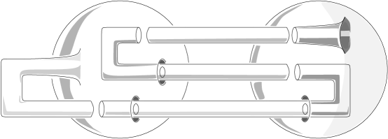
Figure 1: Example 10 in “Quick Trip”

The sphere that is illustrated first appeared in the manuscript [22] by Fox and Milnor, and later as Example 10 in Fox’s “Quick Trip” [21], described in a motion picture form. This knotted sphere is not obtained by the spinning construction [1]. This can be seen as follows. The Alexander polynomial of a spun knot agrees with that of the underlying classical knot since their fundamental groups are isomorphic. The first homology $H_{1}(\tilde{X})$ (called the knot module), of the infinite cyclic cover $\tilde{X}$ of the complement $X$ of the sphere in $S^{4}$ in question, is $\mathbb{Z}[T,T^{-1}]/(2-T)$ as a $\Lambda=\mathbb{Z}[T,T^{-1}]$-module, thus the Alexander polynomial is not symmetric.

Figure 2: Broken surface diagrams

Fox’s Example 11 can be recognized as the same sphere as Example 10 with its orientation reversed. Its Alexander polynomial is $(1-2T)$. Thus the sphere illustrated in Fig. 1 is non-invertible: It is not ambiently isotopic to the same surface with its orientation reversed.

Example 12 of “Quick Trip” has as its knot module $\Lambda/(2-T,1-2T)$. It is obtained from the previous two examples by combining some of their portions. The fact that this ideal is not principal also illustrates the difference between classical knot theory and knotted surfaces. Note that the argument of asymmetric ideals no longer applies to Example 12. It is also interesting to note that this example is in fact the $2$-twist spun trefoil [33], although Zeeman’s twist spin construction appeared later in 1965 [44].

Hillman [24] showed that this knotted sphere was non-invertible using the Farber-Levine pairing. Ruberman [40] used Casson-Gordon invariants to prove the same result, with other new examples of non-invertible knotted spheres. Neither technique applies directly to the same knot with a trivial $1$-handle attached. Kawauchi [31, 32] has generalized the Farber-Levine pairing to higher genus surfaces, showing that such a torus is also non-invertible. The method we survey in this article shows this fact [7] using an invariant defined in a state-sum form from quandle cohomology theory, called the cocycle knot invariant. The cocycle knot invariant has also been used to prove new geometric results [41].

We asked Ruberman if he had proved non-invertibility of the $2$-twist-spun trefoil on his first excursion to the Georgia Topology Conference in 1982. (Incidentally, the first named author also had his topology debute at GTC1982. The second named author debued at GTC1990.) Ruberman told us that the era was correct, although he did not present the result then. His dissertation, however, was inspired by the paper by Sumners [42], which showed, in particular, that any $2$-sphere in $4$-space that contains the Stevedore’s knot as a cross-section is knotted, such as the above examples in “Quick Trip.”

In Section 4 below, we will give the definition of the cocycle invariant for classical knots and for knotted surfaces in $4$-space. Our motivation came from the Jones polynomial and quantum invariants of $3$-manifolds. A common feature of the quantum invariants is the state-sum definition, and it has been asked since their discovery whether such invariants exist in higher dimensions (see [13, 15] for such attempts). We briefly review the state-sum definition of Jones polynomial and a related invariant for triangulated $3$-manifolds — the Dijkgraaf-Witten invariant.

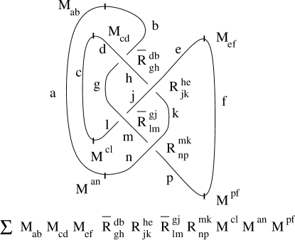
Figure 3: Bracket polynomial of knots

The Bracket Model

The bracket polynomial of a classical knot or link is obtained as follows. The knot is projected generically into the plane, and a height function on the plane is chosen. Let an index set $S=\{1,2\}$ (in general a finite set), whose elements are called spins, be given and fixed. Let ${\cal A}$ denote the set of arcs obtained from the given knot diagram by deleting local maxima, minima, and crossing points. The coloring ${\cal C}$ is a map ${\cal C}:{\cal A}\rightarrow S$.

Boltzmann weights $B(\tau,{\cal C})$ are assigned at minima, maxima, and crossings as follows: Local minima are assigned $M^{ab}$, local maxima are assigned $M_{ab}$, crossings are assigned $R^{ab}_{cd}$ if the over crossing arc has positive slope, or $\overline{R}^{ab}_{cd}$ if the over-crossing arc has negative slope, where each weight is defined with a variable $A$ and $i=\sqrt{-1}$ by

$$M^{ab}=M_{ab}=\left\{\begin{array}[]{ll}iA&\mbox{if \quad$a=0$, $b=1$}\\ (iA)^{-1}&\mbox{if \quad$a=1$, $b=0$}\\ 0&\mbox{otherwise}\end{array}\right.,$$

$$R^{ab}_{cd} = A\delta^{a}_{c}\delta^{b}_{d}+A^{-1}M^{ab}M_{cd},$$

$$\overline{R}^{ab}_{cd} = A^{-1}\delta^{a}_{c}\delta^{b}_{d}+AM^{ab}M_{cd}.$$

Here, $\delta$ denotes Kronecker’s delta. The bracket polynomial, as a polynomial in $A$, is defined by the state-sum

$$\langle K\rangle=\sum_{\cal C}\prod_{\tau}B(\tau,{\cal C}),$$

where the product is taken over all crossings, and the sum is taken over all colorings. The Jones polynomial is obtained from the bracket by normalizing and substituting. Spefically, the quantity ${\mathcal{L}}_{K}(A)=(-A)^{-3w}\langle K\rangle$ is a knot invariant, where the exponent $w$ is the writhe of the diagram $K$, and $V(t)={\mathcal{L}}_{K}(t^{-1/4})$ is the Jones polynomial. In Fig. 3, a colored knot diagram and its Boltzmann weights are depicted. For a given coloring (denoted by lower case letters $a$ through $p$ excluding $i$ ) on arcs, the product of the Boltzmann weights are given at the bottom of the figure. The sum is taken over all colorings, see [29] for details.

The Dijkgraaf-Witten Invariant

Similar state-sum invariants were defined for $3$-manifolds in [16] using group cocycles and the state-sum concept as follows. A combinatorial definition for Chern-Simons invariants with finite gauge groups was given using $3$-cocycles of group cohomology. We follow Wakui’s description, see [43] for more detailed treatments. Let $T$ be a triangulation of an oriented closed $3$-manifold $M$, with $a$ vertices and $n$ tetrahedra. Give an ordering to the set of vertices. Let $G$ be a finite group. Let ${\cal C}:$ $\{$ oriented edges $\}\rightarrow G$ be a map such that (1) for any triangle with vertices $v_{0},v_{1},v_{2}$ of $T$, ${\cal C}(\langle v_{0},v_{2}\rangle)={\cal C}(\langle v_{1},v_{2}\rangle){\cal C}(\langle v_{0},v_{1}\rangle)$, where $\langle v_{i},v_{j}\rangle$ denotes the oriented edge with endpoints $v_{1}$ and $v_{2}$, and (2) ${\cal C}(-e)={\cal C}(e)^{-1}$. Such a map ${\cal C}$ is called a (group) coloring. Let $\alpha:G\times G\times G\rightarrow A$, $(g,h,k)\mapsto\alpha[g|h|k]\in A$, be a $3$-cocycle with values in a multiplicative abelian group $A$, $\alpha\in Z^{3}(G;A)$. The $3$-cocycle condition is written as

$$\alpha[h|k|l]\alpha[gh|k|l]^{-1}\alpha[g|hk|l]\alpha[g|h|kl]^{-1}\alpha[g|h|k]=1.$$

Then the Dijkgraaf-Witten invariant is defined by

$$Z_{M}=\frac{1}{|G|^{a}}\sum_{{\cal C}}\prod_{i=1}^{n}W(\sigma,{\cal C})^{\epsilon_{i}}.$$

Here $a$ denotes the number of the vertices of the given triangulation, $W(\sigma,{\cal C})=\alpha[g|h|k]$ where ${\cal C}(\langle v_{0},v_{1}\rangle)=g$, ${\cal C}(\langle v_{1},v_{2}\rangle)=h$, ${\cal C}(\langle v_{2},v_{3}\rangle)=k$, for the tetrahedron $\sigma=|v_{0}v_{1}v_{2}v_{3}|$ with the ordering $v_{0}<v_{1}<v_{2}<v_{3}$, and $\epsilon=\pm 1$ according to whether or not the orientation of $\sigma$ with respect to the vertex ordering matches the orientation of $M$, see Fig. 4.

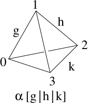
Figure 4: A $3$-cocycle assigned at a triangle

2 Quandles and Quandle Colorings

In this section we define quandles, quandle colorings, and illustrate that counting quandle colorings can be formulated as a state-sum. This definition will help motivate the definition of the quandle cocycle invariants that we will define in Section 4.

A quandle, $X$, is a set with a binary operation $(a,b)\mapsto a*b$ such that

(I) For any $a\in X$, $a*a=a$.

(II) For any $a,b\in X$, there is a unique $c\in X$ such that $a=c*b$.

(III) For any $a,b,c\in X$, we have $(a*b)*c=(a*c)*(b*c).$

A rack is a set with a binary operation that satisfies (II) and (III).

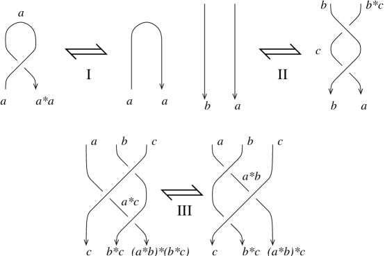
Figure 5: Reidemeister moves and quandle conditions

Racks and quandles have been studied in, for example, [2, 18, 26, 29, 36]. The axioms for a quandle correspond respectively to the Reidemeister moves of type I, II, and III (see Fig. 5 and [18, 29], for example). A function $f:X\rightarrow Y$ between quandles or racks is a homomorphism if $f(a\ast b)=f(a)*f(b)$ for any $a,b\in X$. The following are typical examples of quandles.

• A group $X=G$ with $n$-fold conjugation as the quandle operation: $a*b=b^{-n}ab^{n}$.

• Any set $X$ with the operation $x*y=x$ for any $x,y\in X$ is a quandle called the trivial quandle. The trivial quandle of $n$ elements is denoted by $T_{n}$.

• Let $n$ be a positive integer. For elements $i,j\in\{0,1,\ldots,n-1\}$, define $i\ast j\equiv 2j-i\pmod{n}$. Then $\ast$ defines a quandle structure called the dihedral quandle, $R_{n}$. This set can be identified with the set of reflections of a regular $n$-gon with conjugation as the quandle operation.

• Any $\Lambda(={\mathbb{Z}}[T,T^{-1}])$-module $M$ is a quandle with $a*b=Ta+(1-T)b$, $a,b\in M$, called an Alexander quandle. Furthermore for a positive integer $n$, a mod-$n$ Alexander quandle ${\mathbb{Z}}_{n}[T,T^{-1}]/(h(T))$ is a quandle for a Laurent polynomial $h(T)$. It is finite if the coefficients of the highest and lowest degree terms of $h$ are units in $\mathbb{Z}_{n}$.

Figure 6: Quandle relation at a crossing

Let $X$ be a fixed quandle. Let $K$ be a given oriented classical knot or link diagram, and let ${\cal R}$ be the set of (over-)arcs. The normals are given in such a way that (tangent, normal) matches the orientation of the plane, see Fig. 6. A (quandle) coloring ${\cal C}$ is a map ${\cal C}:{\cal R}\rightarrow X$ such that at every crossing, the relation depicted in Fig. 6 holds. More specifically, let $\beta$ be the over-arc at a crossing, and $\alpha$, $\beta$ be under-arcs such that the normal of the over-arc points from $\alpha$ to $\beta$. Then it is required that ${\cal C}(\gamma)={\cal C}(\alpha)*{\cal C}(\beta)$.

Alternately, a coloring can be described as a quandle homomorphism as follows. Classical knots have fundamental quandles that are defined via generators and relations. The theory of quandle presentations is given a complete treatment in [18]. Specifically, the generators of the fundamental quandle correspond to the arcs in a diagram. The quandle relation $a*b=c$ holds where $a$ is the generator that corresponds to the underarc away from which the normal to the over arc points, $b$ is the generator that corresponds to the overarc, and $c$ corresponds to the underarc towards which the transversal’s normal points, see Fig. 6. A coloring of a classical knot diagram by a quandle $X$ gives rise to a quandle homomorphism from the fundamental quandle to the quandle $X$.

The number $\mbox{Col}_{X}(K)$ of colorings of a knot diagram $K$ by a fixed finite quandle $X$ is a knot invariant, and has a description as a state-sum as follows.

For a finite quandle $X$, consider the set of maps $\{{\cal D}:{\cal R}\rightarrow X\}$ (without the requirement of a quandle coloring). For a given such a map ${\cal D}$, define the Boltzmann weight at a crossing $\tau$, with over-arc $\beta$ whose normal points from the under-arc $\alpha$ to the under-arc $\gamma$, by

$$B(\tau,{\cal D})=\left\{\begin{array}[]{ll}1&{\mbox{\rm if}}\ \ {\cal D}(\alpha)*{\cal D}(\beta)={\cal D}(\gamma)\\ 0&{\mbox{\rm otherwise}}.\end{array}\right.$$

Then the number of quandle colorings is written by a state-sum $\mbox{Col}_{X}(K)=\sum_{{\cal D}}\prod_{\tau}B(\tau,{\cal D})$. We could also use colorings similar to those used in the bracket, or we could write $\mbox{Col}_{X}(K)=\sum_{{\cal C}}\prod_{\tau}B_{1}(\tau,{\cal C})$, where ${\cal C}$ ranges over only quandle colorings ${\cal C}$, and $B_{1}(\tau,{\cal C})\equiv 1$ is a constant function. Either way, it is natural to ask whether we can modify the weights $1$ to a general function.

Fox’s $n$-coloring is a quandle coloring by the dihedral quandle $R_{n}$. The classical result that a knot is non-trivially Fox $p$-colorable if and only if $p|\Delta(-1)$ (where $\Delta(t)$ denotes the Alexander polynomial) has been generalized by Inoue [25] to the following:

Let $\Delta_{K}^{(i)}(T)$ denote the greatest common divisor of all $(n-i-1)$ minor determinants of the presentation matrix for the knot module obtained via the Fox calculus.

Theorem 2.1

[25] Let $p$ be a prime number, $J$ an ideal of the ring $\Lambda_{p}=\mathbb{Z}_{p}[T,T^{-1}]$ and let $Q(K)$ denote a knot quandle. For each $i\geq 0$, put $e_{i}(T)=\Delta_{K}^{(i)}(T)/\Delta_{K}^{(i+1)}(T).$ Then the number of all quandle homomorphisms of the knot quandle $Q(K)$ to the Alexander quandle $\Lambda_{p}/J$ is equal to the cardinality of the module $\Lambda_{p}/J\oplus\oplus_{i=0}^{n-2}\{\Lambda_{p}/(e_{i}(T),J)\}$

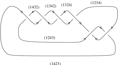
Figure 7: A coloring of $6_{1}$ by $QS_{6}$

Example 2.2

The Alexander quandle $S_{4}=\mathbb{Z}_{2}[T,T^{-1}]/(T^{2}+T+1)$ has four elements that are represented as $0,1,T,$ and $T+1$. This quandle colors both the trefoil ($3_{1}$) and the figure $8$ knot ($4_{1}$) as one can easily see directly or by considering the mod-$2$ reduction of the Alexander polynomials. In either case, the order of $S_{4}$ is $4$ but the determinants are $3$ and $5$, for $3_{1}$ and $4_{1}$, respectively. Thus quandle colorings are more general than Fox colorings.

Example 2.3

The quandle $QS_{6}$ consists of the $4$-cycles $a=(1234)$, $A=(1432)$, $b=(1243)$, $B=(1342)$, $c=(1324)$, and $C=(1423)$ with group conjugation as the quandle operation. Figure 7 illustrates a coloring of the knot $6_{1}$ by $QS_{6}$. This quandle has $R_{3}$ as a quotient quandle. The map $f(a)=f(A)=0$, $f(b)=f(B)=1$, and $f(c)=f(C)=2$ is a quandle homomorphism. The equalizers ($E_{y}=\{x:f(x)=f(y)\}$) are all the two element trivial quandle. Recently, Angela Harris has shown that $QS_{6}$ is not an Alexander quandle of the form $\Lambda_{n}/(h)$ where $h$ is a polynomial.

3 Quandle Homology and Cohomology Theories

In this section, we present twisted quandle homology, which was discussed in [4], and specialize it to the untwisted theory subsequently. Originally, rack homology and homotopy theory were defined and studied in [19], and a modification to quandle homology theory was given in [7] to define a knot invariant in a state-sum form. Then they were generalized to a twisted theory in [4]. Computations are found in [8, 9] and also in [34, 37] by other authors.

Let $\Lambda=\mathbb{Z}[T,T^{-1}]$, and let $C_{n}^{\rm TR}(X)=C_{n}^{\rm TR}(X;\Lambda)$ be the free module over $\Lambda$ generated by $n$-tuples $(x_{1},\dots,x_{n})$ of elements of a quandle $X$. Define a homomorphism $\partial=\partial^{T}_{n}:C_{n}^{\rm TR}(X)\to C_{n-1}^{\rm TR}(X)$ by

$$\partial^{T}_{n}(x_{1},x_{2},\dots,x_{n})$$

$$=\sum_{i=1}^{n}(-1)^{i}\left[T(x_{1},x_{2},\dots,x_{i-1},x_{i+1},\dots,x_{n})\right.$$

$$-\left.(x_{1}\ast x_{i},x_{2}\ast x_{i},\dots,x_{i-1}\ast x_{i},x_{i+1},\dots,x_{n})\right]$$

for $n\geq 2$ and $\partial^{T}_{n}=0$ for $n\leq 1$. We regard that the $i=1$ terms contribute $(1-T)(x_{2},\ldots,x_{n})$. Then $C_{\ast}^{\rm TR}(X)=\{C_{n}^{\rm TR}(X),\partial^{T}_{n}\}$ is a chain complex. For any $\Lambda$-module $A$, let $C_{\ast}^{\rm TR}(X;A)=\{C_{n}^{\rm TR}(X)\otimes_{\Lambda}A,\partial^{T}_{n}\}$ be the induced chain complex, where the induced boundary operator is represented by the same notation. Let $C^{n}_{\rm TR}(X;A)=\mbox{Hom}_{\Lambda}(C_{n}^{\rm TQ}(X),A)$ and define the coboundary operator $\delta=\delta^{n}_{\rm TR}:C^{n}_{\rm TR}(X;A)\to C^{n+1}_{\rm TR}(X;A)$ by $(\delta f)(c)=(-1)^{n}f(\partial c)$ for any $c\in C_{n}^{\rm TQ}(X)$ and $f\in C^{n}_{\rm TR}(X;A)$. Then $C^{\ast}_{\rm TR}(X;A)=\{C^{n}_{\rm TR}(X;A),\delta^{n}_{\rm TR}\}$ is a cochain complex. The $n\/$-th homology and cohomology groups of these complexes are called twisted rack homology group and cohomology group, and are denoted by $H_{n}^{\rm TR}(X;A)$ and $H^{n}_{\rm TR}(X;A)$, respectively.

Let $C_{n}^{\rm TD}(X;A)$ be the subset of $C_{n}^{\rm TR}(X;A)$ generated by $n$-tuples $(x_{1},\dots,x_{n})$ with $x_{i}=x_{i+1}$ for some $i\in\{1,\dots,n-1\}$ if $n\geq 2$; otherwise let $C_{n}^{\rm TD}(X;A)=0$. If $X$ is a quandle, then $\partial^{T}_{n}(C_{n}^{\rm TD}(X;A))\subset C_{n-1}^{\rm TD}(X;A)$ and $C_{\ast}^{\rm TD}(X;A)=\{C_{n}^{\rm TD}(X;A),\partial^{T}_{n}\}$ is a sub-complex of $C_{\ast}^{\rm TR}(X;A)$. Similar subcomplexes $C^{\ast}_{\rm TD}(X;A)=\{C^{n}_{\rm TD}(X;A),\delta_{T}^{n}\}$ are defined for cochain complexes. The $n\/$-th homology and cohomology groups of these complexes are called twisted degeneracy homology group and cohomology group, and are denoted by $H_{n}^{\rm TD}(X;A)$ and $H^{n}_{\rm TD}(X;A)$, respectively.

Put $C_{n}^{\rm TQ}(X;A)=C_{n}^{\rm TR}(X;A)/C_{n}^{\rm TD}(X;A)$ and $C_{\ast}^{\rm TQ}(X;A)=\{C_{n}^{\rm TQ}(X;A),{\partial}^{T}_{n}\}$, where all the induced boundary and coboundary operators are denoted by $\partial={\partial}^{T}_{n}$ and $\delta={\delta}_{T}^{n}$, respectively. A cochain complex $C^{\ast}_{\rm TQ}(X;A)=\{C^{n}_{\rm TQ}(X;A),{\delta}_{T}^{n}\}$ is similarly defined. The $n\/$-th homology and cohomology groups of these complexes are called twisted homology group and cohomology group, and are denoted by

$$H_{n}^{\rm TQ}(X;A)=H_{n}(C_{\ast}^{\rm TQ}(X;A)),\quad H^{n}_{\rm TQ}(X;A)=H^{n}(C^{\ast}_{\rm TQ}(X;A)).$$

The groups of (co)cycles and (co)boundaries are denoted using similar notations.

Example 3.1

The $1$-cocycle condition is written for $\eta\in Z^{1}_{TQ}(X;A)$ as

$$-T\eta(x_{2})+T\eta(x_{1})+\eta(x_{2})-\eta(x_{1}*x_{2})=0,\quad\mbox{or}$$

$$T\eta(x_{1})+(1-T)\eta(x_{2})=\eta(x_{1}*x_{2}).$$

Note that this means that $\eta:X\rightarrow A$ is a quandle homomorphism.

The $2$-cocycle condition is written for $\phi\in Z^{2}_{TQ}(X;A)$ as

$$T[-\phi(x_{2},x_{3})+\phi(x_{1},x_{3})-\phi(x_{1},x_{2})]$$

$$+ [\phi(x_{2},x_{3})-\phi(x_{1}*x_{2},x_{3})+\phi(x_{1}*x_{3},x_{2}*x_{3})]=0\quad\mbox{or}$$

$$T\phi(x_{1},x_{2})+\phi(x_{1}*x_{2},x_{3})$$

$$= T\phi(x_{1},x_{3})+(1-T)\phi(x_{2},x_{3})+\phi(x_{1}*x_{3},x_{2}*x_{3}).$$

The geometric meaning of this condition will become clear in Section 4.

The original untwisted quandle homology is described as a specification of $T=1$. Specifically, in the definition of the boundary homomorphism $\partial^{T}_{n}$, set $T=1$, and define all the cycle, boundary, homology groups similarly. Then use Hom$(\ -\ ;A)$ to define cohomology theory. Thus we assume that the coefficients $A$ simply form an abelian group. We obtain degenerate, rack, and quandle homology groups denoted by $H^{\rm W}_{*}(X;A)$ for $W=D,R,Q$, respectively. Similarly, $H_{\rm W}^{n}(X;A)$ denotes the corresponding cohomology groups. The cohomology theory $H_{\rm R}^{*}$ was defined in [19]. It was seen in [9] that the short exact sequence:

$$0\to C_{n}^{\rm D}(X)\stackrel{{\scriptstyle i}}{{\to}}C_{n}^{\rm R}(X)\stackrel{{\scriptstyle j}}{{\to}}C_{n}^{\rm Q}(X)\to 0$$

gives rise to the following homology long exact sequence:

$$\cdots\stackrel{{\scriptstyle\partial_{\ast}}}{{\to}}H_{n}^{\rm D}(X;A)\stackrel{{\scriptstyle i_{\ast}}}{{\to}}H_{n}^{\rm R}(X;A)\stackrel{{\scriptstyle j_{\ast}}}{{\to}}H_{n}^{\rm Q}(X;A)\stackrel{{\scriptstyle\partial_{\ast}}}{{\to}}H_{n-1}^{\rm D}(X;A)\to\cdots$$

and it was shown in [11] by geometric arguments that the sequence splits in low dimensions. This result was improved upon in [34] by Litherland and Nelson where they showed the following:

Theorem 3.2

[34] The above long exact sequence splits into short exact sequences

$$0{\to}H_{n}^{\rm D}(X;A){\to}H_{n}^{\rm R}(X;A){\to}H_{n}^{\rm Q}(X;A){\to}0.$$

In fact, they construct a projection $p:C_{n}^{\rm R}(X){\to}C_{n}^{\rm D}(X)$ thereby splitting the short exact sequence of chain complexes.

4 Cocycle Knot Invariants

Untwisted Cocycle Invariants

Let $K$ be a classical knot or link diagram. Let a finite quandle $X$, and an (untwisted) quandle $2$-cocycle $\phi\in Z^{2}_{\rm Q}(X;A)$ be given. A (Boltzmann) weight, $B(\tau,{\cal C})$ (that depends on $\phi$), at a crossing $\tau$ is defined as follows. Let ${\cal C}$ denote a coloring ${\cal C}:{\cal R}\rightarrow X$. Let $\beta$ be the over-arc at $\tau$, and $\alpha$, $\gamma$ be under-arcs such that the normal to $\beta$ points from $\alpha$ to $\gamma$, see Fig. 6. Let $x={\cal C}(\alpha)$ and $y={\cal C}(\beta)$. Then define $B(\tau,{\cal C})=\phi(x,y)^{\epsilon(\tau)}$, where $\epsilon(\tau)=1$ or $-1$, if (the sign of) the crossing $\tau$ is positive or negative, respectively. By convention, the crossing in Fig. 6 is positive if the orientation of the under-arc points downward.

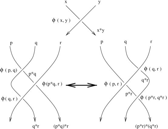
Figure 8: The untwisted $2$-cocycle condition and type III move

The (quandle) cocycle knot invariant is defined by the state-sum expression

$$\Phi(K)=\sum_{{\cal C}}\prod_{\tau}B(\tau,{\cal C}).$$

The product is taken over all crossings of the given diagram $K$, and the sum is taken over all possible colorings. The values of the partition function are taken to be in the group ring ${\bf Z}[A]$ where $A$ is the coefficient group written multiplicatively. The state-sum depends on the choice of $2$-cocycle $\phi$. This is proved [7] to be a knot invariant. Figure 8 shows the invariance of the state-sum under the Reidemeister type III move. The sums of cocycles, equated before and after the move, is the $2$-cocycle condition given in Example 3.1 with the evaluation $T=1$.

The following variations have been considered.

• Lopes [35] observed that the family $\{\prod_{\tau}B(\tau,{\cal C})\}_{\cal C}$ is a knot invariant, without taking summation. In particular, infinite quandles can be used for coloring in this case.

• For a link $L=K_{1}\cup\ldots\cup K_{n}$, let ${\cal T}_{i}$, $i=1,\ldots,n$, be the set of crossings at which the under-arcs belong to the component $K_{i}$. Then it was observed [4] that $\{\sum_{\cal C}\prod_{\tau\in{\cal T}_{i}}B(\tau,{\cal C})\}_{i=1}^{n}$ is a link invariant, strictly stronger than the single state-sum.

Twisted Cocycle Invariants

Let $K$ be an oriented knot diagram with normals. The (underlying) diagram divides the plane into regions. Take an arc $\ell$ from the region at infinity to a region $H$ such that $\ell$ intersects the arcs (missing crossings) of the diagram transversely in finitely many points. The Alexander numbering ${\cal L}(H)$ of a region $H$ is the number of such intersections counted with signs. This does not depend on the choice of an arc $\ell$.

Figure 9: Alexander numbering of a crossing

Let $\tau$ be a crossing. There are four regions near $\tau$, and the unique region from which normals of over- and under-arcs point is called the source region of $\tau$. The Alexander numbering ${\cal L}(\tau)$ of a crossing $\tau$ is defined to be ${\cal L}(R)$ where $R$ is the source region of $\tau$. Compare with [10]. In other words, ${\cal L}(\tau)$ is the number of intersections, counted with signs, between an arc $\ell$ from the region at infinity to $\tau$ approaching from the source region of $\tau$. In Fig. 9, the source region $R$ is the left-most region, and the Alexander numbering of $R$ is $k$, and so is the Alexander numbering of the crossing $\tau$.

Let a classical knot (or link) diagram $K$, a finite quandle $X$, a finite Alexander quandle $A$ be given. A coloring of $K$ by $X$ also is given and is denoted by ${\cal C}$. A twisted (Boltzmann) weight, $B_{T}(\tau,{\cal C})$, at a crossing $\tau$ is defined as follows. Let ${\cal C}$ denote a coloring. Let $\beta$ be the over-arc at $\tau$, and $\alpha$, $\gamma$ be under-arcs such that the normal to $\beta$ points from $\alpha$ to $\gamma$. Let $x={\cal C}(\alpha)$ and $y={\cal C}(\beta)$. Pick a twisted quandle $2$-cocycle $\phi\in Z^{2}_{\rm TQ}(X;A)$. Then define $B_{T}(\tau,{\cal C})=[\phi(x,y)^{\epsilon(\tau)}]^{T^{-{\cal L}(\tau)}}$, where $\epsilon(\tau)=1$ or $-1$, if the sign of $\tau$ is positive or negative, respectively. Here, we use the multiplicative notation of elements of $A$, so that $\phi(x,y)^{-1}$ denotes the inverse of $\phi(x,y)$. Recall that $A$ admits an action by $\mathbb{Z}=\{T^{n}\}$, and for $a\in A$, the action of $T$ on $a$ is denoted by $a^{T}$. To specify the action by ${T^{-{\cal L}(\tau)}}$ in the figures, each region $R$ with Alexander numbering ${\cal L}(R)=k$ is labeled by the power $T^{-k}$ framed with a square, as depicted in Fig. 9.

The state-sum, or a partition function, is the expression

$$\Phi_{T}(K)=\sum_{{\cal C}}\prod_{\tau}B_{T}(\tau,{\cal C}).$$

The product is taken over all crossings of the given diagram, and the sum is taken over all possible colorings. The value of the weight $B_{T}(\tau,{\cal C})$ is in the coefficient group $A$ written multiplicatively. Hence the value of the state-sum is in the group ring ${\bf Z}[A]$.

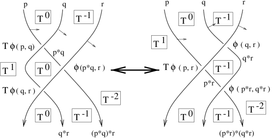
Figure 10: The twisted $2$-cocycle condition and type III move

It was proved in [5] that $\Phi_{T}(K)$ is a knot invariant, called the (quandle) twisted cocycle invariant. Figure 10 depicts the invariance under the type III move, where the left-most region is assumed to have Alexander numbering $-1$. The sum over all these cocycles, equated before and after the move, gives the $2$-cocycle condition written in Example 3.1.

Cocycle Invariants for Knotted Surfaces

The state-sum invariant is defined in an analogous way for oriented knotted surfaces in $4$-space using their projections and diagrams in $3$-space. Specifically, the above steps can be repeated as follows, for a fixed finite quandle $X$ and a knotted surface diagram $K$.

Figure 11: Colors at double curves and $3$-cocycle at a triple point

• The diagrams consist of double curves and isolated branch and triple points [14]. Along the double curves, the coloring rule is defined using normals in the same way as classical case, as depicted in the left of Fig. 11.

• The Alexander numbering ${\cal L}$ of regions divided by a given diagram is defined similarly.

• The source region $R$ and the Alexander numbering ${\cal L}(\tau)={\cal L}(R)$ are defined for a triple point $\tau$ using orientation normals.

• The sign $\epsilon(\tau)$ of a triple point $\tau$ is defined [14] in such a way that it is positive if and only if the normals ot top, middle, bottom sheets, in this order, match the orientation of $3$-space.

• For a coloring ${\cal C}$, the Boltzman weight at a triple point $\tau$ is defined by $B_{T}(\tau,{\cal C})=$ $[\theta(x,y,z)^{\epsilon(\tau)}]^{T^{-{\cal L}(\tau)}}$, where $\theta$ is a $3$-cocycle, $\theta\in Z^{3}_{\rm TQ}(X;A)$. In the right of Fig. 11, the triple point $\tau$ is positive, and ${\cal L}(\tau)=0$, so that $B_{T}(\tau,{\cal C})=\theta(p,q,r)$.

• The state-sum is defined by $\Phi_{T}(K)=\sum_{{\cal C}}\prod_{\tau}B_{T}(\tau,{\cal C}).$

By checking the analogues of Reidemeister moves for knotted surface diagrams, called Roseman moves, it was shown in [5] that $\Phi_{T}(K)$ is an invariant, called the (twisted quandle) cocycle invariant of knotted surfaces.

Similarly, the state-sum invariant in the untwisted case was defined earlier in [6] and [7]. In the untwisted case, there is no Alexander numbering, and the Boltzmann weight at a triple point is simply the quantity $B(\tau,{\cal C})=\theta(x,y,z)^{\epsilon(\tau)}$ where $x,y,z$ are the colors on the source regions of the bottom, middle, and top sheets at the triple points.

In all of these cases, the value of the state-sum invariant depends only on the cohomology class represented by the defining cocycle. In particular, a coboundary will simply count the number of colorings of a knot or knotted surface by the quandle $X$.

Applications

Two important topological applications have been obtained using the cocycle invariants.

• The $2$-twist spun trefoil $K$ and its orientation-reversed counterpart $-K$ have shown to have distinct cocycle invariants using a cocycle in $Z^{3}_{Q}(R_{3};\mathbb{Z}_{3})$, providing a proof that $K$ is non-invertible [7].

  The higher genus surfaces obtained from $K$ by adding arbitrary number of trivial $1$-handles are also non-invertible, since such handle additions do not alter the cocycle invariant.

  We note, again, that this result in higher genus cases is not immediately obtained from [24, 40], although higher genus generalizations of the Farber-Levine pairing [32] can be used.

• The projection of the $2$-twist spun trefoil was shown to have at least four triple points [41].

  The same cocycle group $Z^{3}_{Q}(R_{3};\mathbb{Z}_{3})$, but a different cocycle found in [37] was used.

5 Virtual Knots and Quandle Homology

In this section, we describe $2$-dimensional quandle homology classes as cobordism classes of quandle colored virtual knot diagrams. See [11, 19, 20, 23] for more general geometric descriptions of homology classes.

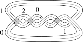
Figure 12: A colored virtual knot

Consider an untwisted quandle homology class of a quandle $X$, and represent the class by $\eta\in Z_{2}^{\rm Q}(X)$. Write $\eta$ as a sum of $2$-chains $\eta=\sum_{j}\epsilon_{j}(a_{j},b_{j})$ where $\epsilon_{j}=\pm 1$. For each $j$ with $\epsilon_{j}=1$, consider a positive crossing diagram in which the over-arc is colored $b_{j}$ and the under-arc away from which the normal to the over arc points is colored $a_{j}$. Similarly, when $\epsilon_{j}=-1$ we consider a negative crossing of the same form. The boundary of the chain is $\pm(a_{j}-a_{j}*b_{j})$ which is the difference in the colors on the under-arcs. Since $\eta$ is a cycle these boundary terms cancel over the sum of the crossings.

Thus to represent the $2$-cycle, we take a disjoint union of colored crossings, and join the end-point arcs together when they have the correct orientation and the same color. The arcs are joined together formally, and the joining need not occur on a planar diagram, obtaining a colored “virtual knot diagram.” Virtual knots have been popularized by L.H. Kauffman who has found, for example, that the diagram in Fig. 12 has trivial Jones polynomial. A virtual knot can be regarded as a knot on a surface [27].

Conversely, a colored virtual knot diagram represents a $2$-cycle. In Fig. 12, such a diagram colored with $R_{3}=\{0,1,2\}$ is depicted. The colored crossings in shaded squares, from left to right, represent $2$-chains $(0,1)$, $(1,2)$, and $-(1,0)$, respectively, and therefore, this diagram shows that the $2$-chain $(0,1)+(1,2)-(1,0)$ is a $2$-cocycle. The unshaded crossings between bands can be regarded as virtual crossings. These bands connecting shaded squares correspond to identifying matching boundaries in the above construction. Some remarks are in order.

• There is a one-to-one correspondence [11] between (1) quandle colored virtual knot diagrams modulo the virtual Reidemeister moves and colored cobordisms, and (2) $2$-dimensional quandle homology classes.

• This geometric representations were used to estimate the rank of rack homology groups in [20, 23] for some racks and quandles.

• This was also used to show that a certain long exact sequence splits [11] at low dimensions, as mentioned in Section 4.

• The $2$-dimensional regions near crossings in classical diagrams can also be colored to represent $3$-cycles. Such colorings were used in [39] to give an alternate proof that left- and right handed trefoils are not equivalent.

• The cocycle invariants can be interpreted as a formal sum of the Kronecker product between a fixed cocycle and such cycles constructed above represented by colored diagrams. Such an interpretation was used in [12] to evaluate the cocycle invariants.

• Twisted cycles have a similar interpretation, but the consistency of Alexander numbering requires care.

• The untwisted homology group $H_{2}^{\rm Q}(R_{3})$ is trivial. Thus the cycle $(0,1)+(1,2)-(1,0)$ is a boundary. Meanwhile, the fundamental quandle [30] of the virtual knot in Fig. 12 can be computed to be $R_{3}$. Thus we have the interesting situtation in which a knot, with any coloring by its fundamental quandle elements, is null-homologous in the $2$-dimensional cycle group of its fundamental quandle.

6 Constructions of Cocycles from Extension Theory of Quandles

The first constructions of quandle cocycles were a combination of hand and computer calculations [7, 8]. Here we summarize two important cases. To describe cocycles, denote the characteristic function by

$$\chi_{a}(x)=\left\{\begin{array}[]{ll}1&{\mbox{\rm if }}\ a=x\\ 0&{\mbox{\rm if }}\ a\neq x\end{array}\right.,$$

where $a$, $x$ are $n$-tuples of elements of a quandle $X$.

• For the Alexander quandle $S_{4}=\mathbb{Z}_{2}[T,T^{-1}]/(T^{2}+T+1)$, the $\mathbb{Z}_{2}$-valued function

  $$\phi=\sum_{a\neq b\;a,b\neq T}\chi_{a,b}$$

  represents a non-trivial cohomology class in $H^{2}_{\rm Q}(S_{4};\mathbb{Z}_{2})\cong\mathbb{Z}_{2}$.

• It was computed that $H^{3}_{\rm Q}(R_{3};\mathbb{Z}_{3})\cong\mathbb{Z}_{3}$ and a generator is given by

  $$\theta=-\chi_{(0,1,0)}+\chi_{(0,2,0)}-\chi_{(0,2,1)}+\chi_{(1,0,1)}+\chi_{(1,0,2)}+\chi_{(2,0,2)}+\chi_{(2,1,2)}\in Z^{3}_{\rm Q}(R_{3};\mathbb{Z}_{3}).$$

In [7] it was mentioned that the trefoil ($3_{1}$) and the figure-eight knot $(4_{1})$ have non-trivial cocycle invariants with the cocycle $\phi$. It was also shown that the $2$-twist spun trefoil is not invertible using the $3$-cocycle $\theta$. This was proven using similar techniques in [39]. Recently, Satoh and Shima [41] have shown that any diagram for the $2$-twist spun trefoil has at least 4 triple points using a $3$-cocycle in $Z^{3}_{\rm Q}(R_{3};\mathbb{Z}_{3})$ discovered by Mochizuki [37]. Mochizuki [37], Litherland and Nelson [34] have developed more techniques for computing quandle homology and cohomology.

For quantum invariants, solutions (R-matrices) to the Yang-Baxter equations were discovered by calculations first, and then Drinfeld [17] developed a theory of quantum groups whose representations gave rise to R-matrices. This construction is seen as an obstruction to co-commutativity satisfying the next order (the Yang-Baxter) relation, or, deformation theory of an algebraic structure giving rise to a solution to a higher order relation. Considering analogies between group and quandle cohomology theories, it is, then, natural to seek such methods of finding cocycles in deformation and extension theories of quandles. An extension theory of quandles was developed in [5] for the twisted case as follows (see also [4, 12]), in analogy with the group cohomology theory (one sees that the following is in parallel to Chapter IV of [3]).

• Let $X$ be a quandle and $A$ be an Alexander quandle, so that $A$ admits an action by $\mathbb{Z}$ whose generator is denoted by $T$. Let $\phi\in Z^{2}_{\rm TQ}(X;A)$. Let $AE(X,A,\phi)$ be the quandle defined on the set $A\times X$ by the operation $(a_{1},x_{1})*(a_{2},x_{2})=(a_{1}*a_{2}+\phi(x_{1},x_{2}),x_{1}*x_{2})$.

• The above defined operation $*$ on $A\times X$ indeed defines a quandle $AE(X,A,\phi)=(A\times X,*)$, which is called an Alexander extension of $X$ by $(A,\phi)$.

• Let $X$ be a quandle and $A$ be an Alexander quandle. Recall that $\eta\in Z^{1}_{\rm TQ}(X;A)$ implies that $\eta:X\rightarrow A$ is a quandle homomorphism. Let $0\rightarrow N\stackrel{{\scriptstyle i}}{{\rightarrow}}G\stackrel{{\scriptstyle p}}{{\rightarrow}}A\rightarrow 0$ be an exact sequence of $\mathbb{Z}[T,T^{-1}]$-module homomorphisms among Alexander quandles. Let $s:A\rightarrow G$ be a set-theoretic section (i.e., $ps=$id_A) with the “normalization condition” $s(0)=0$. Then $s\eta:X\rightarrow G$ is a mapping, which is not necessarily a quandle homomorphism. We measure the failure by $2$-cocycles. Since $p[Ts\eta(x_{1})+(1-T)s\eta(x_{2})]=p[s\eta(x_{1}*x_{2})]$ for any $x_{1},x_{2}\in A$, there is $\phi(x_{1},x_{2})\in N$ such that

  $$Ts\eta(x_{1})+s\eta(x_{2})=i\phi(x_{1},x_{2})+[Ts\eta(x_{2})+s\eta(x_{1}*x_{2})].$$

  This defines a function $\phi\in C^{2}_{\rm TQ}(X;N)$. Then it was shown that $\phi\in Z^{2}_{\rm TQ}(X;N)$.

• Let $s^{\prime}:A\rightarrow G$ be another section, and $\phi^{\prime}\in Z^{2}_{\rm TQ}(X;N)$ be a $2$-cocycle determined by

  $$Ts^{\prime}\eta(x_{1})+s^{\prime}\eta(x_{2})=i\phi^{\prime}(x_{1},x_{2})+[Ts^{\prime}\eta(x_{2})+s^{\prime}\eta(x_{1}*x_{2})].$$

  Then it was shown that $[\phi]=[\phi^{\prime}]\in H^{2}_{\rm TQ}(X;N)$.

• It was shown that if $[\phi]=0\in H^{2}_{\rm TQ}(X;N)$, then $\phi$ extends to a quandle homomorphism to $G$, i.e., there is a quandle homomorphism $\eta^{\prime}:X\rightarrow G$ such that $p\eta^{\prime}=\eta$.

The above results were summarized as

Theorem 6.1

[5] The obstruction to extending $\eta:X\rightarrow A$ to a quandle homomorphism $X\rightarrow G$ lies in $H^{2}_{\rm TQ}(X;N)$.

Conversely, we have the following.

Lemma 6.2

[5] Let $X$, $E$ be quandles, and $A$ be an Alexander quandle. Suppose there exists a bijection $f:E\rightarrow A\times X$ with the following property. There exists a function $\phi:X\times X\rightarrow A$ such that for any $e_{i}\in E$ ($i=1,2$), if $f(e_{i})=(a_{i},x_{i})$, then $f(e_{1}*e_{2})=(a_{1}*a_{2}+\phi(x_{1},x_{2}),x_{1}*x_{2})$. Then $\phi\in Z^{2}_{\rm TQ}(X;A)$.

This lemma implies that under the same assumption we have $E=AE(X,A,\phi)$, where $\phi\in Z^{2}_{\rm TQ}(X;A)$, and by identifying such quandles, we obtain cocycles as desired. We identify such examples, and include a proof, as it provides explicit formulas of cocycles.

Let $\Lambda_{p}=\mathbb{Z}_{p}[T,T^{-1}]$ for a positive integer $p$ (or $p=0$, in which case $\Lambda_{p}$ is understood to be $\Lambda=\mathbb{Z}[T,T^{-1}]$). Note that since $T$ is a unit in $\Lambda_{p}$, $\Lambda_{p}/(h)$ for a Laurent polynomial $h\in\Lambda_{p}$ is isomorphic to $\Lambda_{p}/(T^{n}h)$ for any integer $n$, so that we may assume that $h$ is a polynomial with a non-zero constant (without negative exponents of $T$).

Lemma 6.3

[5] Let $h\in\Lambda_{p^{m}}$ be a polynomial with leading and constant coefficients invertible, or $h=0$. Let $\bar{h}\in\Lambda_{p^{m-1}}$ and $\tilde{h}\in\Lambda_{p}$ be such that $\bar{h}\equiv h\ \mbox{mod}\ (p^{m-1})$ and $\tilde{h}\equiv h\ \mbox{mod}\ (p)$, respectively (in other words, $\bar{h}$ is $h$ with its coefficients reduced modulo $p^{m-1}$, and $\tilde{h}$ is $h$ with its coefficients reduced modulo $p$). Then the quandle $E=\Lambda_{p^{m}}/({h})$ satisfies the conditions in Lemma 6.2 with $X=\Lambda_{p^{m-1}}/(\bar{h})$ and $A=\Lambda_{p}/(\tilde{h})$.

In particular, $\Lambda_{p^{m}}/({h})$ is an Alexander extension of $\Lambda_{p^{m-1}}/(\bar{h})$ by $\Lambda_{p}/(\tilde{h})$:

$$\Lambda_{p^{m}}/(h)=AE(\Lambda_{p^{m-1}}/(\bar{h}),\ \Lambda_{p}/(\tilde{h}),\ \phi),$$

for some $\phi\in Z^{2}_{\rm TQ}(\Lambda_{p^{m-1}}/(\bar{h});\Lambda_{p}/(\tilde{h}))$.

Proof. Let $A\in\mathbb{Z}_{p^{m}}$. Represent $A$ in $p^{m}$-ary notation as

$$A=\sum_{i=0}^{m-1}A_{i}p^{i}$$

where $A_{i}\in\{0,\ldots,p-1\}.$ Since $p$ is fixed throughout, we represent $A$ by the sequence

$$[A_{m-1},A_{m-2},A_{m-3},\ldots,A_{0}].$$

Define $\overline{A}=[A_{m-2},\ldots,A_{0}].$ Observe that $A\equiv\overline{A}\pmod{p^{m-1}}$, and $A\equiv A_{0}\pmod{p}$.

Let $\hat{\pi}:\mathbb{Z}_{p^{m}}\rightarrow\mathbb{Z}_{p^{m-1}}$ be the map defined by $\hat{\pi}(A)=\overline{A}$. We obtain a short exact sequence:

$$0\rightarrow\mathbb{Z}_{p}\stackrel{{\scriptstyle\hat{\imath}}}{{\rightarrow}}\mathbb{Z}_{p^{m}}\stackrel{{\scriptstyle\hat{\pi}}}{{\rightarrow}}\mathbb{Z}_{p^{m-1}}\rightarrow 0$$

where $\hat{\imath}(A)=[A,0,\dots,0]$. There is a set-theoretic section $\mathbb{Z}_{p^{m}}\stackrel{{\scriptstyle\hat{s}}}{{\leftarrow}}\mathbb{Z}_{p^{m-1}}$ defined by $\hat{s}[A_{m-2},\dots,A_{0}]=[0,A_{m-2},\dots,A_{0}].$ The map $\hat{s}$ satisfies $\hat{\pi}\hat{s}={\rm id}$ and $\hat{s}(0)=0$.

For a polynomial $L(T)\in\Lambda_{p^{m}}=\mathbb{Z}_{p^{m}}[T,T^{-1}]$, write

$$L(T)=\sum_{j=-n}^{k}[A_{j,m-1},A_{j,m-2},\ldots,A_{j,0}]T^{j}.$$

Define

$$\overline{L}(T)=\sum_{j=-n}^{k}[A_{j,m-2},\ldots,A_{j,0}]T^{j}\in\Lambda_{p^{m-1}},$$

and

$$\tilde{L}(T)=\sum_{j=-n}^{k}A_{j,m-1}T^{j}\in\Lambda_{p}.$$

There is a one-to-one correspondence $f:\Lambda_{p^{m}}\rightarrow\Lambda_{p}\times\Lambda_{p^{m-1}}$ given by $f(L)=(\tilde{L},\overline{L})$. We have a short exact sequence of rings:

$$0\rightarrow\mathbb{Z}_{p}[T,T^{-1}]\stackrel{{\scriptstyle i}}{{\rightarrow}}\mathbb{Z}_{p^{m}}[T,T^{-1}]\stackrel{{\scriptstyle\pi}}{{\rightarrow}}\mathbb{Z}_{p^{m-1}}[T,T^{-1}]\rightarrow 0$$

with a set theoretic section $\mathbb{Z}_{p^{m}}[T,T^{-1}]\stackrel{{\scriptstyle s}}{{\leftarrow}}\mathbb{Z}_{p^{m-1}}[T,T^{-1}]$ where $i$, $\pi$ and $s$ are the natural maps induced by $\hat{i}$, $\hat{\pi}$ and $\hat{s}$, respectively. Note that for $L\in\Lambda_{p^{m}}=\mathbb{Z}_{p^{m}}[T,T^{-1}]$ we have $\overline{L}=\pi(L)$, and the section $s:\Lambda_{p^{m-1}}\rightarrow\Lambda_{p^{m}}$ is defined by the formula

$$s\left(\sum_{j=-n}^{k}[A_{j,m-2},\ldots,A_{j,0}]T^{j}\right)=\sum_{j=-n}^{k}[0,A_{j,m-2},\ldots,A_{j,0}]T^{j}.$$

For $L,M\in\Lambda_{p^{m}}$, let

$$s(\overline{L})*s(\overline{M})=\sum_{j}[F_{j,m-1},\ldots,F_{j,0}]T^{j}\in\Lambda_{p^{m-1}}.$$

If $L=\sum_{j}A_{j}T^{j}$, and $M=\sum_{j}B_{j}T^{j}$, then

$$L*M=B_{-n}T^{-n}+\sum_{j=-n+1}^{k+1}(A_{j-1}-B_{j-1}+B_{j})T^{j}=\sum_{j=-n}^{k}C_{j}T^{j}.$$

Furthermore,

$$\overline{L}*\overline{M} = [B_{-n,m-2},\ldots,B_{-n,0}]T^{-n}$$

$$+ \sum_{j=-n+1}^{k+1}\left([A_{j-1,m-2},\ldots,A_{j-1,0}]-[B_{j-1,m-2},\ldots,B_{j-1,0}]+[B_{j,m-2},\ldots,B_{j,0}]\right)T^{j}$$

and write the right-hand side by $\sum_{j=-n}^{k}D_{j}T^{j}$. Note that $D_{j}$’s are well-defined integers, not only elements of $\mathbb{Z}_{p^{m-2}}$. If $D_{j}$ is positive, then $F_{j,m-1}=0$, and if $D_{j}$ is negative, then $F_{j,m-1}=p-1$. Hence

$$f(L*M)=(\tilde{L}*\tilde{M}+\phi(\overline{L},\overline{M}),\overline{L}*\overline{M}),$$

where

$$\phi(\overline{L},\overline{M})=\sum_{j=-n}^{k}F_{j,m-1}.$$

This concludes the case $h=0$.

Now let $h(T)\in\mathbb{Z}_{p^{m}}[T]$ be a polynomial with leading and constant coefficients being invertible in $\mathbb{Z}_{p}$. Let $(h)$ denote the ideal generated by $h$. Since $i(\tilde{h})\subset(h)$, we obtain a short exact sequence of quotients:

$$0\rightarrow\mathbb{Z}_{p}[T,T^{-1}]/(\tilde{h})\stackrel{{\scriptstyle\overline{\imath}}}{{\rightarrow}}\mathbb{Z}_{p^{m}}[T,T^{-1}]/(h)\stackrel{{\scriptstyle\overline{\pi}}}{{\rightarrow}}\mathbb{Z}_{p^{m-1}}[T,T^{-1}]/(\overline{h})\rightarrow 0$$

with a set-theoretic section $\mathbb{Z}_{p^{m}}[T,T^{-1}]/(h)\stackrel{{\scriptstyle\overline{s}}}{{\leftarrow}}\mathbb{Z}_{p^{m-1}}[T,T^{-1}]/(\overline{h}).$ Thus we obtain a twisted cocycle

$$\phi:\mathbb{Z}_{p^{m-1}}[T,T^{-1}]/(\overline{h})\times\mathbb{Z}_{p^{m-1}}[T,T^{-1}]/(\overline{h})\rightarrow\mathbb{Z}_{p}[T,T^{-1}]/(\tilde{h})\quad\hbox{\rule{6.0pt}{6.0pt}}$$

Since $R_{n}=\Lambda_{n}/(T+1)$, we have the following.

Corollary 6.4

The dihedral quandle $E=R_{p^{m}}$, where $p,m$ are positive integers with $m>1$, satisfies the conditions in Lemma 6.2 with $X=R_{p^{m-1}}$ and $A=R_{p}$.

In particular, $R_{p^{m}}$ is an Alexander extension of $R_{p^{m-1}}$ by $R_{p}$: $R_{p^{m}}=AE(R_{p^{m-1}},\ R_{p},\ \phi)$, for some $\phi\in Z^{2}_{\rm TQ}(R_{p^{m-1}};R_{p})$.

Example 6.5

Let $X=R_{3}$ and $A=R_{3}$, then the proof of Lemma 6.3 gives an explicit $2$-cocycle $\phi$ as follows. For $\phi(r_{1},r_{2})=\phi(1,2)$, for example, one computes

$$r_{1}*r_{2}=[0,1]*[0,2]=2[0,2]-[0,1]=3=3\cdot 1+0=[1,0],$$

Hence $\phi(0,2)=1$. In terms of the characteristic function, the cocycle $\phi$ contains the term $\chi_{0,2}$. By computing the quotients for all pairs, one obtains

$$\phi=\chi_{0,2}+\chi_{1,2}+2\chi_{1,0}+2\chi_{2,0}.$$

The same argument was applied to $R_{\infty}$ to show that the quandle $R_{\infty}$ is an Alexander extension of $R_{n}$ by $R_{\infty}$, for any positive integer $n$.

Similar techniques give us untwisted cocycles [4], with explicit formulas for these $2$-cocycles as follows. In this case, the extension is called an abelian extension, denoted by $E=E(X,A,\phi)$ for $\phi\in Z^{2}_{\rm Q}(X;A)$, and the quandle operation on $E=A\times X$ is defined by $(a_{1},x_{1})*(a_{2},x_{2})=(a_{1}+\phi(x_{1},x_{2}),x_{1}*x_{2})$.

• For any positive integers $q$ and $m$, $E=\mathbb{Z}_{q^{m+1}}[T,T^{-1}]/(T-1+q)$ is an abelian extension $E=E(\mathbb{Z}_{q^{m}}[T,T^{-1}]/(T-1+q),\mathbb{Z}_{q},\phi)$ of $X=\mathbb{Z}_{q^{m}}[T,T^{-1}]/(T-1+q)$ for some cocycle $\phi\in Z^{2}_{\rm Q}(X;\mathbb{Z}_{q})$.

• For any positive integer $q$ and $m$, the quandle $E=\mathbb{Z}_{q}[T,T^{-1}]/(1-T)^{m+1}$ is an abelian extension of $X=\mathbb{Z}_{q}[T,T^{-1}]/(1-T)^{m}$ over $\mathbb{Z}_{q}$: $E=E(X,\mathbb{Z}_{q},\phi)$, for some $\phi\in Z^{2}_{\rm Q}(X;\mathbb{Z}_{q})$.

Furthermore, for untwisted $2$-cocycles, an interpretation of the cocycle knot invariant was given [4] as an obstruction to extending a given coloring of a knot diagram by a quandle $X$ to a coloring by an abelian extension $E$. Similar interpretations for twisted case or knotted surface case are unknown.

Ohtsuki [38] defined a new cohomology theory for quandles and an extension theory, together with a list of problems in the subject.

Acknowledgements

We gratefully acknowledge the contributions of our collaborators in these projects: Mohammed Elhamdadi, Daniel Jelsovsky, Seiichi Kamada, Louis Kauffman, Laurel Langford, and Marina Nikiforou. We thank the organizers of the 2001 GTC for their hard work and for allowing us the opportunity to present these results. As we were finishing this paper we received a copy of the survey [28]. We are pleased to refer the reader to that paper as well.

References

- [1] Artin, E., Zur Isotopie zweidimensionalen Flächen im , Abh. Math. Sem. Univ. Hamburg 4 (1926) 174–177
- [2] Brieskorn, E., Automorphic sets and singularities, in “Contemporary math.” 78 (1988) 45–115
- [3] Brown, K. S., Cohomology of groups, Graduate Texts in Mathematics, 87. Springer-Verlag, New York-Berlin (1982)
- [4] Carter, J, Scott, Elhamdadi, M., Nikiforou, M., Saito. M., Extensions of quandles and cocycle knot invariants, Preprint http://xxx.lanl.gov/math/abs/GT0107021
- [5] Carter, J, Scott, Elhamdadi, M., Saito. M., Twisted Quandle homology theory and cocycle knot invariants, Preprint http://xxx.lanl.gov/math/abs/GT0108051
- [6] Carter, J.S.; Jelsovsky, D.; Kamada, S.; Langford, L.; Saito, M., State-sum invariants of knotted curves and surfaces from quandle cohomology, Electron. Res. Announc. Amer. Math. Soc. 5 (1999) 146-156
- [7] Carter, J.S.; Jelsovsky, D.; Kamada, S.; Langford, L.; Saito, M., Quandle cohomology and state-sum invariants of knotted curves and surfaces, Preprint http://xxx.lanl.gov/abs/math.GT/9903135
- [8] Carter, J.S.; Jelsovsky, D.; Kamada, S.; Saito, M., Computations of quandle cocycle invariants of knotted curves and surfaces,, Advances in math 157 (2001) 36-94
- [9] Carter, J.S.; Jelsovsky, D.; Kamada, S.; Saito, M., Quandle homology groups, their betti numbers, and virtual knots,, J. of Pure and Applied Algebra 157 (2001), 135-155
- [10] Carter, J.S.; Kamada, S.; Saito, M., Alexander numbering of knotted surface diagrams, Proc. A.M.S. 128 (2000) 3761–3771
- [11] Carter, J.S.; Kamada, S.; Saito, M., Geometric interpretations of quandle homology, J. of Knot Theory and its Ramifications 10 (2001) 345-358
- [12] Carter, J.S.; Kamada, S.; Saito, M., Diagrammtic computations for quandles and cocycle knot invariants,, Contemporary Math. Proceedings of a conference on quantum topology, held in San Francisco, 1999, to appear. available at http://xxx.lanl.gov/abs/math.GT/0102092.
- [13] Carter, J.S.; Kauffman, L.H.; Saito, M., Structures and diagrammatics of four-dimensional topological lattice field theories, Adv. Math. 146 (1999) 39-100
- [14] Carter, J.S.; Saito, M., Knotted surfaces and their diagrams, Surveys and monographs, Amer. Math. Soc. 55 (1998)
- [15] Crane, L.; Kauffman, L.H.; Yetter, D.N., State-sum invariants of -manifolds, J. Knot Theory Ramifications 6 (1997) 177-234
- [16] Dijkgraaf, R.; Witten, E., Topological gauge theories and group cohomology, Comm. Math. Phys. 129 (1990)
- [17] Drinfel’d, V.G., Quantum groups, in “Proceedings of the International Congress of Mathematicians (Berkeley, Calif., 1986)” Amer. Math. Soc., Providence, RI, 1987 798-820
- [18] Fenn, R.; Rourke, C., Racks and links in codimension two, J. Knot Theory Ramifications 1 (1992) 343-406
- [19] Fenn, R.; Rourke, C.; Sanderson, B., James bundles and applications,, Preprint http://www.maths.warwick.ac.uk/∼bjs/
- [20] Flower, J., Cyclic Bordism and Rack Spaces, Ph.D. Dissertation, Warwick (1995)
- [21] Fox, R.H., A quick trip through knot theory, in “Topology of 3-manifolds and related topics” (Georgia, 1961), Prentice-Hall (1962) 120–167
- [22] Fox, R.H. ; Milnor, J.W., Singularities of 2-spheres in 4-space, Manuscript (Circa 1957)
- [23] Greene, M. T., Some Results in Geometric Topology and Geometry,, Ph.D. Dissertation, Warwick (1997)
- [24] Hillman, J.A., Finite knot modules and the factorization of certain simple knots, Math. Ann. 257 (1981) 261–274
- [25] Inoue, A. , Quandle homomorphisms of knot quandles to Alexander quandles, J. Knot Theory Ramifications 10 (2001) 813–821
- [26] Joyce, D., A classifying invariant of knots, the knot quandle, J. Pure Appl. Alg. 23 (1982) 37–65
- [27] Kamada, N.; Kamada, S., Abstract link diagrams and virtual knots, J. Knot Theory Ramifications 9 (2000) 93–106
- [28] Kamada, S., Knot invariants derived from quandles and racks, preprint (2001)
- [29] Kauffman, L.H., Knots and Physics, Series on knots and everything 1 World Scientific (1991)
- [30] Kauffman, L. H., Virtual knot theory, European J. Combin 20 (1999) 7 663–690
- [31] Kawauchi, A., Three dualities on the integral homology of infinite cyclic coverings of manifolds, Osaka J. Math. 23 (1986) 633-651
- [32] Kawauchi, A., The first Alexander modules of surfaces in 4-sphere, in “Algebra and Topology” (Taejon, 1990), Proc. KAIST Math. Workshop, 5, KAIST, Taejon, Korea (1990) 81–89
- [33] LitherLand, R., Letter to Cameron Gordon: Example 12 is the 2-twist spun trefoil,
- [34] Litherland, R.A.; Nelson, S.,, The Betti numbers of some finite racks, Preprint http://xxx.lanl.gov/abs/math.GT/0106165
- [35] Lopes, P., Quandles at finite temperatures I, Preprint http://xxx.lanl.gov/abs/math.QA/0105099
- [36] Matveev, S., Distributive groupoids in knot theory (Russian), Math. USSR-Sbornik 47 (1982) 73–83
- [37] Mochizuki, T., Some calculations of cohomology groups of finite Alexander quandles, Preprint
- [38] Ohtsuki, T. (ed), Problems on invariants of knots and -manifolds, Proeprint
- [39] Rourke, C.; Sanderson, B, There are two 2-twist-spun trefoils, Preprint http://xxx.lanl.gov/abs/math.GT/0006062
- [40] Ruberman, D., Doubly slice knots and the Casson-Gordon invariants, Trans. Amer. Math. Soc. 279 (1983) 569–588
- [41] Satoh, S.; Shima, A., The 2-twist spun trefoil has the triple number four, preprint
- [42] Sumners, D.W., Invertible Knot Cobordisms, in “Proceedings of the 1968 Georgia Topology Conference” Topology of Manifolds, ed. Cantrell, J. C, and Edwards, C.H. Jr. Markham (1970)
- [43] Wakui, M., On Dijkgraaf-Witten invariants for -manifolds, Osaka J. Math. 29 (1992) 675-696
- [44] Zeeman, E.C., Twisting spun knots, Trans. Amer. Math. Soc. 115 (1965) 471-495