Trapped modes in a waveguide with a thick obstacle

1. Introduction

The problem of finding necessary and sufficient conditions for the existence of trapped modes in waveguides has been known since 1943, [8]. The problem is the following: consider an infinite strip $M$ in $\mathbb{R}^{2}$ (or an infinite cylinder with the smooth boundary in $\mathbb{R}^{n}$). The spectrum of the (positive) Laplacian (with either Dirichlet or Neumann boundary conditions) acting on this strip is easily computable via the separation of variables; the spectrum is absolutely continuous and equals $[\nu_{0},+\infty)$. Here, $\nu_{0}$ is the first threshold, i.e. eigenvalue of the cross-section of the cylinder (so $\nu_{0}=0$ in the case of Neumann conditions). Let us now consider the domain $\tilde{\Omega}$ (the waveguide) which is a smooth compact perturbation of $M$ (for example, we insert an obstacle in $M$). The essential spectrum of the Laplacian acting on $\tilde{\Omega}$ still equals $[\nu_{0},+\infty)$, but there may be additional eigenvalues (so-called trapped modes; the number of these trapped modes can be quite large, see examples in [9] and [6]). So, the problem is in finding conditions for the existence or absence of such eigenvalues and studying them when they exist. It is customary to distinguish between two situations: the Dirichlet boundary conditions (corresponding to the so-called quantum waveguides) and the Neumann boundary conditions (corresponding to the acoustic waveguides). In the Dirichlet case the first threshold $\nu_{0}>0$, so the eigenvalues can occur outside the essential spectrum. Such eigenvalues (not embedded into the essential spectrum) are stable under small perturbations, and thus they occur in a wide range of situations (see e.g. [3]). On the contrary, in the Neumann case any eigenvalue is embedded into the continuous spectrum and is very unstable. Therefore, the existence of such eigenvalues is usually due to some symmetry (obvious or hidden) of the situation. In [2] it was shown that if the obstacle is symmetric about the axis of the strip, then for a wide range of obstacles there is (at least one) eigenvalue. Later, in [1] more conditions, necessary as well as sufficient for the existence of eigenvalues were established. Also, in that paper the example of a hidden symmetry resulting in the existence of an eigenvalue was given. Once the existence of eigenvalues is established, it is natural to ask how many of them there are and how they behave. In the case of a symmetric obstacle the problem splits into two problems on the half of $\tilde{\Omega}$ (obtained by cutting the initial waveguide along its axis); one of these problems corresponds to the additional Dirichlet conditions on the added boundary; the other has additional Neumann conditions. The essential spectrum of the first sub-problem starts at the first non-zero threshold $\nu_{1}>0$ (in the case of the strip of width $2$ which we will consider in this paper, $\nu_{1}=\pi^{2}/4$), and the second sub-problem still has essential spectrum growing from zero (see next section for more details). Paper [5] studied what happens if the symmetric obstacle becomes long (in the direction of the axis of the strip). It is proved there that the number of eigenvalues of the Dirichlet sub-problem below $\nu_{1}$ is of the order of the length of the obstacle. In the present paper we study another regime of the asymptotic behaviour of such eigenvalues: suppose that the obstacle is a rectangle placed symmetrically on the axis of the strip (see figure 1).

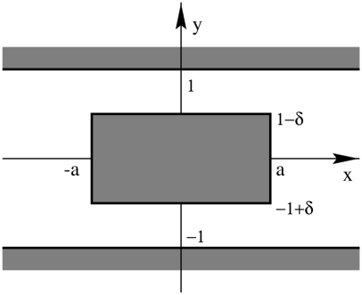
Figure 1.

Let the width of the strip be $2$, the length of the rectangle (in the direction of the axis of the strip) be $2a$ and the distance from the rectangle to the sides of the waveguide (in the direction orthogonal to the axis) be $\delta$. When $\delta=0$, the domain degenerates to the union of two semistrips. We are interested in the behaviour of the eigenvalues which lie below the first non-zero threshold $\nu_{1}=\pi^{2}/4$ when $\delta\downarrow 0$, in particular, the rate at which they tend to the threshold.

The choice of the rectangle as an obstacle is motivated by the following considerations: suppose for simplicity that $0<a<1$. Then, if the obstacle has the shape as in figure 2,

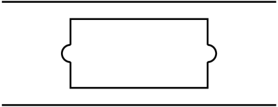
Figure 2.

the (unique) eigenvalue will stay away from the threshold $\nu_{1}$ (this can be proved using the same method as in [2]). On the other hand, if the obstacle has the shape as in figure 3,

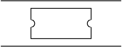
Figure 3.

it was shown in [1] that for small enough $\delta$ there are no eigenvalues below $\nu_{1}$ at all. The case of a rectangle is an intermediate one: for any $\delta$ there is a unique eigenvalue which converges towards $\nu_{1}$ as $\delta\to 0$. This makes the case of a rectangular obstacle such an interesting one. A slightly different problem about the rate of convergence of an eigenvalue to a threshold (in the context of a quantum waveguide) was considered in [4] and [7], and that problem turned out to be quite difficult (so that one has to work a lot even to get the correct order of convergence). Our problem, on the contrary, is relatively easy, and one can get the first asymptotic term without too much difficulty (in fact, only the first transversal mode contributes towards the first asymptotic term). We think that one can also obtain the second asymptotic term (by studying further transversal modes), but we have not done this in our paper. The result we have obtained is rather surprising in the sense that the rate of convergence of an eigenvalue towards the threshold depends on whether $a$ is an integer or not. We postpone the precise formulation of the result until the next section.

The proof of our result will go along the standard lines. To estimate the eigenvalue from above, we will produce the test-function (or functions, if we have several eigenvalues). To obtain the precise asymptotic constant, the test-function has to be chosen with great care. In order to estimate the eigenvalue from below, we use the technique of estimating quadratic forms, similar to the method of transference of excess energy (see [1]). There is a small difference between our approach and the method of [1]. Namely, instead of comparing the integrals of the function along different sub-regions of $\tilde{\Omega}$ (which was the key tool in [1]), in our paper we compare such integrals with values of the function in certain points.

The rest of the paper is organised in the following way: in the next section we give some preliminary information and formulate the main theorem 2.1; sections 3-5 are devoted to the proof of this theorem. For the convenience of the reader we discuss first (in the section 3) the easiest case when $a<1$. Section 4 deals with the case $a=1$ (so that in both these sections we have only one eigenvalue). Finally, in section 5 we explain which changes should be made in the proof when $a$ is arbitrary (and there are several eigenvalues).

Acknowledgement We are very grateful to D. Vassiliev and M. Levitin for helpful suggestions and comments.

2. Preliminaries

We consider the domain $\tilde{\Omega}=(-\infty,\infty)\times(-1,1)\setminus(-a,a)\times(-(1-\delta),1-\delta)$, $0<a$, $0<\delta<1$. The spectrum of $-\Delta$ with Neumann boundary conditions on $\tilde{\Omega}$ is the interval $[0,+\infty)$. To make the study of the eigenvalues easier, we split $L^{2}(\tilde{\Omega})$ into several subspaces invariant with respect of the action of $-\Delta$. First, let $\Omega$ be the half of $\tilde{\Omega}$: $\Omega=(-\infty,\infty)\times(0,1)\setminus(-a,a)\times(0,1-\delta)$. It is well known (see [2]) that if we consider the operator $L$ which acts as $-\Delta$ on $\Omega$ with Dirichlet boundary conditions on $\{y=0\}$ and Neumann boundary conditions on the rest of the boundary $\partial\Omega$, then eigenvalues of $L$ are at the same time eigenvalues of the Neumann Laplacian on $\tilde{\Omega}$. Moreover, since the essential spectrum of $L$ is $[\pi^{2}/4,+\infty)$, we can study eigenvalues below $\nu_{1}:=\pi^{2}/4$ using the variational approach. It is also convenient to make the further reduction of the domain and consider two problems on $\Omega^{\prime}:=(0,\infty)\times(0,1)\setminus(0,a)\times(0,1-\delta)$: one problem, called $L_{D}$, has Dirichlet conditions on $\{x=0\}\cup\{y=0\}$ and Neumann conditions elsewhere; the other problem, called $L_{N}$, has Dirichlet conditions on $\{y=0\}$ and Neumann conditions elsewhere (see [5] for more details of this decomposition). Then $\sigma(L)=\sigma(L_{D})\cup\sigma(L_{N})$, i.e. the spectrum of $L$ is the union of spectra of $L_{D}$ and $L_{N}$. Let $\lambda_{1}\leq\dots\leq\lambda_{n}$ be the eigenvalues of $L$ lying below $\nu_{1}$. Using the approach of [5], together with the test-function from [2], it is easy to show that $n=-[-a]$ (this will also follow from the proof of our main theorem). Moreover, if $n$ is even, then half of these eigenvalues come from $L_{N}$, and another half comes from $L_{D}$. If $n$ is odd, then the spare eigenvalue is due to $L_{N}$. It is also known that the eigenvalues coming from $L_{N}$ and $L_{D}$ are alternating and that $\lambda_{1}\in\sigma(L_{N})$. Thus, the top eigenvalue $\lambda_{n}$ is an eigenvalue of $L_{N}$ if and only if $n$ is odd. If we fix $a$ and let $\delta\to 0$, then all but the last eigenvalue remain bounded away from $\nu_{1}$, i.e. $\lambda_{n-1}<C<\nu_{1}$ uniformly over $\delta$ (see [5]). On the other hand, $\lambda_{n}\to\nu_{1}$ as $\delta\to 0$. Now we can formulate our main result.

Theorem 2.1.

If $a\not\in\mathbb{N}$, then

(2.1) $$\lambda_{n}=\frac{\pi^{2}}{4}-M(a)\delta^{2}+O(\delta^{3})$$

as $\delta\to 0$, where

(2.2) $$M(a)=\pi^{2}\tan^{2}\left(\frac{\pi\{a\}}{2}\right)=\left\{\begin{array}[]{ll}\pi^{2}\tan^{2}\left(\frac{\pi a}{2}\right)&\textrm{$2l<a<2l+1,$}\\ \pi^{2}\cot^{2}\left(\frac{\pi a}{2}\right)&\textrm{$2l+1<a<2l+2$.}\end{array}\right.$$

Here $\{a\}:=a-[a]$ is the fractional part of $a$. If $a\in\mathbb{N}$, then

(2.3) $$\lambda_{n}=\frac{\pi^{2}}{4}-M(a)\delta^{2/3}+O(\delta^{4/3})$$

as $\delta\to 0$, where

(2.4) $$M(a)=\left(\frac{\pi^{2}}{a}\right)^{2/3}.$$

The rest of the paper is devoted to the proof of this theorem.

3. $a<1$

In this case there is only one eigenvalue (coming from $L_{N}$), and we denote this eigenvalue by $\lambda$. Also, $M(a)=\pi^{2}\tan^{2}\bigl{(}\frac{\pi a}{2}\bigr{)}$. Obviously, (2.1) is equivalent to the following two inequalities:

(3.1) $$\lambda\leq\frac{\pi^{2}}{4}-M(a)\delta^{2}+O(\delta^{3})$$

and

(3.2) $$\lambda\geq\frac{\pi^{2}}{4}-M(a)\delta^{2}-O(\delta^{3}).$$

The strategy of the proof will be quite standard for problems of this sort: to prove (3.1), we will construct the test-function $\phi$ satisfying Dirichlet conditions at $\{x=0\}$ for which the Rayleigh quotient

(3.3) $$Q(\phi):=\frac{\int_{\Omega^{\prime}}|\nabla\phi|^{2}dxdy}{\int_{\Omega^{\prime}}|\phi|^{2}dxdy}=\frac{\pi^{2}}{4}-M(a)\delta^{2}+O(\delta^{3}),$$

and to prove (3.2), we will estimate the quadratic form of $L_{N}$ from below. It is relatively easy to construct the test-function $\phi$ for which

(3.4) $$Q(\phi)=\frac{\pi^{2}}{4}-K\delta^{2}-O(\delta^{3}),$$

but the constant $K$ is worse than $M(a)$. For example, let us denote by

(3.5) $$\eta_{k}(y):=\sqrt{2}\sin\frac{(2k-1)\pi y}{2}$$

($k\geq 1$) the normalized eigenfunctions of the cross-section of the strip at infinity. Then if we choose

(3.6) $$\phi(x,y)=\begin{cases}\eta_{1}(y)e^{-\delta(x-a)},&x\geq a\\ \eta_{1}(y),&x\leq a,\end{cases}$$

this function will satisfy (3.4) with $K=\pi^{2}a-1<M(a)$. In order to get the precise constant, we have to correct the function (3.6) in the region above the obstacle. This correction is not obvious, and in order to understand it, we will first prove (3.2). To begin with, we decompose $\Omega^{\prime}$ into two parts:

(3.7) $$\Omega_{l}:=(0,a)\times(1-\delta,1)$$

and

(3.8) $$\Omega_{r}:=(a,+\infty)\times(0,1).$$

The estimate of the quadratic form will be different in $\Omega_{l}$ and $\Omega_{r}$. In each of these regions we will use certain one-dimensional results to obtain the estimates. The first lemma is rather trivial; it will take care of $\Omega_{r}$.

Lemma 3.1.

For any function $\varphi\in C^{1}(\mathbf{R^{+}})$ and any $m>0$ we have:

(3.9) $$m\varphi^{2}(0)\leq\int_{0}^{\infty}\left(\varphi^{\prime}(x)^{2}+m^{2}\varphi^{2}(x)\right)dx.$$

with equality only when $\varphi(x)=Ce^{-mx}$.

Proof.

Taking into account that

$$\varphi^{2}(0)=-\int_{0}^{\infty}\frac{d}{dx}(\varphi^{2}(x))dx=-2\int_{0}^{\infty}\varphi(x)\varphi^{\prime}(x)dx,$$

we see that (3.9) is equivalent to

$$\int_{0}^{\infty}(\varphi^{\prime}(x)+m\varphi(x))^{2}dx\geq 0,$$

which makes both statements of lemma obvious. ∎

The second lemma will help us to deal with $\Omega_{l}$; this lemma is slightly more subtle.

Lemma 3.2.

Let $0<a<1$ and $f\in C^{2}[0,a],\,f^{\prime}(0)=0$. Then

(3.10) $$\int_{0}^{a}\left(\frac{df}{dx}\right)^{2}dx-\frac{\pi^{2}}{4}\int_{0}^{a}f^{2}(x)dx+\frac{\sqrt{M(a)}\,f^{2}(a)}{2}\geq 0,$$

where

(3.11) $$M(a)=\pi^{2}\tan^{2}\left(\frac{\pi a}{2}\right).$$

Moreover, equality is reached in (3.10) if

(3.12) $$f(x)=C\cos\left(\frac{\pi x}{2}\right).$$

Proof.

Without loss of generality we can assume $f$ satisfies the extra boundary condition

(3.13) $$f^{\prime}(a)=-\frac{\sqrt{M(a)}\,f(a)}{2}.$$

Indeed, given any function $f$ we can choose another function $g$ such that $g$ satisfies (3.13) and the difference of the left hand sides of (3.10) for $f$ and $g$ is arbitrarily small.

We now note that

(3.14) $$\int_{0}^{a}\left(\frac{df}{dx}\right)^{2}dx+\frac{\sqrt{M(a)}\,f^{2}(a)}{2}$$

is the quadratic form of $-\frac{d^{2}}{dx^{2}}$ with the boundary conditions $f^{\prime}(0)=0,f^{\prime}(a)=-\frac{\sqrt{M(a)}\,f(a)}{2}$.

The eigenvalues of this operator are the values of $\mu^{2}$, where $\mu$ satisfy

(3.15) $$\mu\tan(\mu a)=\frac{\sqrt{M(a)}}{2},$$

corresponding eigenfunctions being $\cos(\mu x)$. Therefore, the first eigenvalue equals $\frac{\pi^{2}}{4}$ if and only if $M(a)$ is given by (3.11). This finishes the proof of the lemma. ∎

Now we will prove (3.2). To do this, it is enough to show that whenever $u\in C^{\infty}(\Omega^{\prime})$, $u(x,0)=0$, $\frac{\partial u}{\partial x}(0,y)=0$, $\frac{\partial u}{\partial y}(x,1)=0$ the following inequality is satisfied:

(3.16) $$\int\!\!\!\int_{\Omega^{\prime}}|\nabla u|^{2}dxdy-\left(\frac{\pi^{2}}{4}-M(a)\delta^{2}-O(\delta^{3})\right)\int\!\!\!\int_{\Omega^{\prime}}|u|^{2}dxdy\geq 0$$

where $M(a)=\pi^{2}\tan^{2}\left(\frac{\pi a}{2}\right)$. Let us decompose the LHS of (3.16) as

(3.17) $$\begin{split}&\left(\int\!\!\!\int_{\Omega_{l}}|\nabla u|^{2}dxdy-\frac{\pi^{2}}{4}\int\!\!\!\int_{\Omega_{l}}|u|^{2}dxdy\right)\\ +&\left(\int\!\!\!\int_{\Omega_{r}}|\nabla u|^{2}dxdy-\frac{\pi^{2}}{4}\int\!\!\!\int_{\Omega_{r}}|u|^{2}dxdy\right)\\ +&\left(M(a)\delta^{2}+O(\delta^{4})\right)\int_{\Omega}|u|^{2}dxdy\\ =&:L(u)+R(u)+\left(M(a)\delta^{2}+O(\delta^{4})\right)\int_{\Omega}|u|^{2}dxdy\end{split}$$

(the definitions of $\Omega_{l}$ and $\Omega_{r}$ are given in (3.7) and (3.8)). The main idea of the proof is the following: it is obvious that $R(u)>0$; moreover, there is a certain extra amount of energy in $\Omega_{r}$ to spare. We wish to transfer this excess of energy into $\Omega_{l}$ using the information of one-dimensional problems, similar to the approach in [1]. However, if we do it precisely in the same way as in [1], the estimate we obtain will be too rough. Therefore, instead we transform the excess of energy of $u$ over $\Omega_{r}$ into an extra positive term involving the values of $u$ on the boundary between $\Omega_{r}$ and $\Omega_{l}$. To be more precise, we will show that

(3.18) $$R(u)\geq\frac{\sqrt{M(a)}}{2}\int_{1-\delta}^{1}|u(a,y)|^{2}dy$$

and

(3.19) $$L(u)+\frac{\sqrt{M(a)}}{2}\int_{1-\delta}^{1}|u(a,y)|^{2}dy\geq 0,$$

which obviously would lead to (3.16).

We start by examining $R(u)$ in more details. Since $u(x,0)=0$ and $\frac{\partial u}{\partial y}(x,1)=0$, we can decompose $u$ in the Fourier series when $x\geq a$:

(3.20) $$u(x,y)=\sum_{k=1}^{\infty}u_{k}(x)\eta_{k}(y)$$

($\eta_{j}$ is defined in (3.5)) After simple computations we obtain:

$$\int\!\!\!\int_{\Omega_{r}}|\nabla u|^{2}=\sum_{k=1}^{\infty}\int_{a}^{\infty}\left(u_{k}^{\prime}(x)\right)^{2}dx+\frac{\pi^{2}}{4}\sum_{k=1}^{\infty}(2k-1)^{2}\int_{a}^{\infty}u_{k}^{2}(x)dx$$

and

$$\int\!\!\!\int_{\Omega_{r}}|u|^{2}dxdy=\sum_{k=1}^{\infty}\int_{a}^{\infty}u_{k}^{2}(x)dx.$$

These formulae imply

(3.21) $$\begin{split}R(u)&=\sum_{k=1}^{\infty}\int_{a}^{\infty}\left(u_{k}^{\prime}(x)\right)^{2}dx+\frac{\pi^{2}}{4}\sum_{k=1}^{\infty}(2k-1)^{2}\int_{a}^{\infty}u_{k}^{2}(x)dx\\ &-\frac{\pi^{2}}{4}\sum_{k=1}^{\infty}\int_{a}^{\infty}u_{k}^{2}(x)dx+M(a)\delta^{2}\sum_{k=1}^{\infty}\int_{a}^{\infty}u_{k}^{2}(x)\\ &\geq\sum_{k=1}^{\infty}\int_{a}^{\infty}\left(u_{k}^{\prime}(x)\right)^{2}dx+M(a)\delta^{2}\sum_{k=1}^{\infty}\int_{a}^{\infty}u_{k}^{2}(x)dx\end{split}$$

when $\delta$ is small enough. Now lemma 3.1 implies

(3.22) $$R(u)\geq\sqrt{M(a)}\,\delta\sum_{k=0}^{\infty}u_{k}^{2}(a).$$

On the other hand, the RHS of (3.18) is

(3.23) $$\begin{split}&\frac{\sqrt{M(a)}}{2}\int_{1-\delta}^{1}|u(a,y)|^{2}dy\\ &=\frac{\sqrt{M(a)}}{2}\sum_{k=1}^{\infty}u_{k}^{2}(a)\int_{1-\delta}^{1}2\sin^{2}\left(\frac{\pi}{2}(2k-1)y\right)dy\\ &=\frac{\sqrt{M(a)}}{2}\sum_{k=1}^{\infty}u_{k}^{2}(a)\bigl{(}\delta+\frac{\sin\left(\pi\delta(2k-1)\right)}{\pi(2k-1)}\bigr{)}\leq\sqrt{M(a)}\delta\sum_{k=1}^{\infty}u_{k}^{2}(a),\end{split}$$

which, together with (3.22), proves (3.18). Equation (3.19) follows immediately if we apply lemma 3.2 to the function $u(\cdot,y)$ and then integrate the result over $y$. This finishes the proof of (3.2).

In order to construct the test-function satisfying (3.3), we try to change all inequalities in the proof of the lower bound into equalities. In other words, we need to have equalities in (3.19), (3.22), and (3.21). The lemmas explain what should we do to get equalities in (3.19) and (3.22). In order to get equality (at least up to terms $O(\delta^{3})$) in (3.21), we have to leave only the first Fourier coefficient in (3.20). This leads to the following test-function:

(3.24) $$\phi(x,y)=\left\{\begin{array}[]{ll}\cos\left(\frac{\pi a}{2}\right)e^{-\sqrt{M(a)}\,\delta(x-a)}\sin\left(\frac{\pi y}{2}\right)&\textrm{$x\geq a$,}\\ \cos\left(\frac{\pi x}{2}\right)\sin\left(\frac{\pi y}{2}\right)&\textrm{$x\leq a$.}\end{array}\right.$$

One can check that this function indeed gives us equality up to $O(\delta^{3})$ everywhere where it matters, and so it satisfies (3.3) which proves (3.1). The proof of the theorem in the case $a<1$ is thus finished.

4. $a=1$

As before, the inequality (2.3) is equivalent to the following two inequalities:

(4.1) $$\lambda\leq\frac{\pi^{2}}{4}-M(a)\delta^{2/3}+O(\delta^{4/3})$$

and

(4.2) $$\lambda\geq\frac{\pi^{2}}{4}-M(a)\delta^{2/3}-O(\delta^{4/3}).$$

We start by producing the test-function $\phi(x,y)$ with the Rayleigh quotient equal to the RHS of (4.1). Such a function is given by

(4.3) $$\phi(x,y)=\left\{\begin{array}[]{ll}e^{-\pi^{2/3}\delta^{1/3}(x-1)}\sin\left(\frac{\pi y}{2}\right)&\textrm{$x\geq 1$,}\\ \left(\cos(\mu)\right)^{-1}\cos(\mu x)\sin\left(\frac{\pi y}{2}\right)&\textrm{$x\leq 1$,}\end{array}\right.$$

where $\mu=\frac{\pi}{2}-\pi^{1/3}\delta^{2/3}$. A straightforward (though rather lengthy) computation shows that the Rayleigh quotient of this function indeed satisfies

(4.4) $$Q(\phi)=\frac{\pi^{2}}{4}-M(a)\delta^{2/3}+O(\delta^{4/3}),$$

which proves (4.1). Another way of seeing that (4.4) holds is to read the proof of (4.2) and check that the function $\phi$ changes all inequalities in it into equalities.

Now we give a proof of (4.2). The proof is quite similar to that of (3.2). The biggest change is that instead of Lemma 3.2, in the case $a=1$ we have the following result:

Lemma 4.1.

Let $f\in C^{2}[0,1]$ and $f^{\prime}(0)=0$. Then for all small enough positive $\delta$

(4.5) $$\int_{0}^{1}\left(\frac{df}{dx}\right)^{2}dx-\left(\frac{\pi^{2}}{4}-M\delta^{2/3}-C_{1}\delta^{4/3}\right)\int_{0}^{1}f^{2}(x)dx+\frac{\sqrt{M}f^{2}(1)}{2\delta^{2/3}}\geq 0,$$

where

(4.6) $$M:=M(1)=\pi^{4/3}$$

and $C_{1}$ is a constant, the precise value of which is not important. Moreover, there exists another constant $C_{2}$, such that for

(4.7) $$g(x)=\cos(\mu x)$$

with $\mu^{2}=\frac{\pi^{2}}{4}-\pi^{4/3}\delta^{2/3}$, the inequality in the opposite direction is satisfied, namely:

(4.8) $$\int_{0}^{1}\left(\frac{dg}{dx}\right)^{2}dx-\left(\frac{\pi^{2}}{4}-M\delta^{2/3}-C_{2}\delta^{4/3}\right)\int_{0}^{1}g^{2}(x)dx+\frac{\sqrt{M}g^{2}(1)}{2\delta^{2/3}}\leq 0.$$

Proof.

The proof follows similar lines to those of Lemma 3.2. Without loss of generality we can assume that $f$ satisfies the extra boundary condition

$$f^{\prime}(1)=-\frac{\sqrt{M}\,f(1)}{2\delta^{2/3}}.$$

Then

$$\int_{0}^{1}\left(\frac{df}{dx}\right)^{2}dx+\frac{\sqrt{M}\,f^{2}(1)}{2\delta^{2/3}}$$

is the quadratic form of the operator $-\frac{d^{2}}{dx^{2}}$ with boundary conditions

$$f^{\prime}(0)=0,\qquad f^{\prime}(1)=-\frac{\sqrt{M}\,f(1)}{2\delta^{2/3}}.$$

We therefore need to prove that the first eigenvalue of

(4.9) $$-f^{\prime\prime}(x)=\mu^{2}f(x),\qquad f^{\prime}(0)=0,\qquad f^{\prime}(1)=-\frac{\sqrt{M}\,f(1)}{2\delta^{2/3}}$$

equals $\frac{\pi^{2}}{4}-M\delta^{2/3}+O(\delta^{4/3})$ (this indeed would prove both statements of lemma). The eigenvalues of (4.9) are the values of $\mu_{j}^{2}$ where $\mu_{j}$ are solutions to

(4.10) $$\mu\tan(\mu)=\frac{\sqrt{M}}{2\delta^{2/3}};$$

the corresponding eigenfunctions are $\cos(\mu_{j}x)$. Therefore, we need to make sure that

(4.11) $$\sqrt{\frac{\pi^{2}}{4}-M\delta^{2/3}}\tan\left(\sqrt{\frac{\pi^{2}}{4}-M\delta^{2/3}}\right)=\frac{\sqrt{M}}{2\delta^{2/3}}+O(1).$$

The LHS of (4.11) is

$$\frac{\pi}{2}\frac{\pi}{M\delta^{2/3}}+O(1)=\frac{\pi^{2}}{2M\delta^{2/3}}+O(1).$$

This is precisely the RHS of (4.11) iff $M$ is given by (4.6). ∎

We will now prove (4.2). To do this it is enough to show that for arbitrary $u\in C^{\infty}(\Omega^{\prime})$ such that $u(x,0)=\frac{\partial u}{\partial y}(x,1)=\frac{\partial u}{\partial x}(0,y)=0$, we have

(4.12) $$\int\!\!\!\int_{\Omega^{\prime}}|\nabla u|^{2}dxdy-\left(\frac{\pi^{2}}{4}-M\delta^{2/3}-O(\delta^{4/3})\right)\int\!\!\!\int_{\Omega^{\prime}}|u|^{2}dxdy\geq 0.$$

The LHS of (4.12) can be rewritten as

$$\begin{split}&\left(\int\!\!\!\int_{\Omega_{l}}|\nabla u|^{2}dxdy-\left(\frac{\pi^{2}}{4}-M\delta^{2/3}-O(\delta^{4/3})\right)\int\!\!\!\int_{\Omega_{l}}|u|^{2}dxdy\right)\\ +&\left(\int\!\!\!\int_{\Omega_{r}}|\nabla u|^{2}dxdy-\left(\frac{\pi^{2}}{4}-M\delta^{2/3}-O(\delta^{4/3})\right)\int\!\!\!\int_{\Omega_{r}}|u|^{2}dxdy\right)\\ =&:L(u)+R(u).\end{split}$$

Similar to Section 3, we will show that

(4.13) $$R(u)\geq\frac{\sqrt{M}}{2\delta^{2/3}}\int_{1-\delta}^{1}|u(1,y)|^{2}dy$$

and

(4.14) $$L(u)+\frac{\sqrt{M}}{2\delta^{2/3}}\int_{1-\delta}^{1}|u(1,y)|^{2}dy\geq 0.$$

The proof of (4.13) is absolutely analogous to the proof of (3.18), and we will skip it. In order to prove (4.14), it is sufficient to show that

(4.15) $$\begin{split}\int\!\!\!\int_{\Omega_{l}}\left(\frac{\partial u}{\partial x}\right)^{2}dxdy&-\left(\frac{\pi^{2}}{4}-M\delta^{2/3}-C_{1}\delta^{4/3}\right)\int\!\!\!\int_{\Omega_{l}}|u|^{2}dxdy\\ &+\frac{\sqrt{M}}{2\delta^{2/3}}\int_{1-\delta}^{1}|u(1,y)|^{2}dy\geq 0\end{split}$$

for some choice of the constant $C_{1}$. This follows immediately if we apply Lemma 4.1 to the function $u(\cdot,y)$ and then integrate over $y$. The proof of (4.2) is therefore complete. The careful look at the proof together with the second part of Lemma 4.1 shows that the choice of the test-function (4.3) indeed changes all the inequalities into equalities, and so (4.1) is proved. This finishes the proof of our theorem in the case $a=1$.

5. Arbitrary $a$

Consider now the case of arbitrary $a$. The main difference between this case and the case $a\leq 1$ is the fact that now we have to take care of several test-functions, using the mini-max principle. The cases of integer and non-integer $a$ require slightly different approach as well as the cases of even and odd $[a]$. We consider in details the case of non-integer $a$ with even integer part and prove the theorem in this case. Proof of the other cases is similar, and we will not give it here. So, let us assume that $[a]=2l$, $l\in\mathbb{N}$, $a\not\in\mathbb{N}$. Then, as we have mentioned already, the number of eigenvalues $n=2l+1$, and the top eigenvalue $\lambda_{2l+1}$ comes from the Neumann problem $L_{N}$. This problem has exactly $l+1$ eigenvalues (the other $l$ eigenvalues are due to $L_{D}$). As before, we construct the test-functions to prove the upper bound

(5.1) $$\lambda_{2l+1}\leq\frac{\pi^{2}}{4}-M(a)\delta^{2}+O(\delta^{3})$$

and estimate the quadratic form to prove the lower bound

(5.2) $$\lambda_{2l+1}\geq\frac{\pi^{2}}{4}-M(a)\delta^{2}-O(\delta^{3}).$$

More precisely, in order to prove (5.1) we will construct $l+1$ functions $\phi_{1},\dots,\phi_{l+1}\in H^{1}(\Omega^{\prime})$, $\phi_{j}(x,0)=\frac{\partial\phi_{j}}{\partial x}(0,y)=\frac{\partial\phi_{j}}{\partial y}(x,1)=0$ such that every non-trivial linear combination $\phi=\sum_{j=1}^{l+1}\alpha_{j}\phi_{j}$ satisfies (3.3). As in section 3, it is relatively easy to construct test-functions which satisfy (3.3) with a weaker constant. So, once again we will start with proving the lower bound and this proof will give us the recipe for choosing the optimal test-functions. Taking into account that we are estimating the eigenvalue number $l+1$, the variational formulation of (5.2) is the following: for every set $u_{1},\dots,u_{l+1}\in C^{\infty}(\Omega^{\prime})$, $u_{j}(x,0)=0$, $\frac{\partial u_{j}}{\partial x}(0,y)=0$, $\frac{\partial u_{j}}{\partial y}(x,1)=0$ there exist constants $\alpha_{j}$, not all zeros ($1\leq j\leq l+1$), such that if $u=\sum_{j=1}^{l+1}\alpha_{j}u_{j}$, then $Q(u)\geq\frac{\pi^{2}}{4}-M(a)\delta^{2}-O(\delta^{4})$. The proof of this statement goes similarly to the proof from section 3, but we need to make two modifications. First of all, instead of lemma 3.2 we use the following lemma:

Lemma 5.1.

Let $2l<a<2l+1,l\in\mathbb{N}$ and let $f_{1},\dots,f_{l+1}\in C^{2}[0,a]$ satisfy $f_{j}^{\prime}(0)=0$. Then there exist constants $\alpha_{j}$ not all zeros ($1\leq j\leq l+1$), such that for the linear combination $f=\sum_{j=1}^{l+1}\alpha_{j}f_{j}$ the following inequality is satisfied:

(5.3) $$\int_{0}^{a}\left(\frac{df}{dx}\right)^{2}dx-\frac{\pi^{2}}{4}\int_{0}^{a}f^{2}(x)dx+\frac{\sqrt{M(a)}\,f^{2}(a)}{2}\geq 0,$$

where

(5.4) $$M(a)=\pi^{2}\tan^{2}\left(\frac{\pi a}{2}\right).$$

Moreover, inequality in the other direction is reached in (5.3) for any linear combination of the following functions:

(5.5) $$f_{j}(x)=\cos(\mu_{j}x),\qquad 1\leq j\leq l+1,$$

where $\mu_{j}$ are the first $(l+1)$ solutions to

(5.6) $$\mu_{j}\tan(\mu_{j}a)=\frac{\pi}{2}\tan\left(\frac{\pi a}{2}\right),$$

with $\mu_{l+1}=\frac{\pi}{2}$.

Proof.

The proof of this lemma is similar to the proof of Lemma 3.2. First of all we notice that without loss of generality we can assume that $f_{j}$ satisfy the additional boundary condition $\qquad f_{j}^{\prime}(a)=-\frac{\sqrt{M(a)}\,f_{j}(a)}{2}$. Then the statement of the lemma is equivalent to the fact that the $(l+1)$st eigenvalue of the problem

(5.7) $$-f^{\prime\prime}(x)=\mu^{2}f(x),\qquad f^{\prime}(0)=0,\qquad f^{\prime}(a)=-\frac{\sqrt{M(a)}\,f(a)}{2}$$

is $\frac{\pi^{2}}{4}$ and the functions (5.5) are the first $(l+1)$ eigenfunctions. As in the proof of Lemma 3.2 the eigenvalues of (5.7) are the values of $\mu_{j}^{2}$, where $\mu_{j}$ are (positive) solutions to

(5.8) $$\mu_{j}\tan(\mu_{j}a)=\frac{\sqrt{M(a)}}{2}=\frac{\pi}{2}\tan\left(\frac{\pi a}{2}\right),\qquad\mu_{1}<\mu_{2}<\dots$$

Obviously, $\mu_{j}=\pi/2$ solves (5.8), and we just have to find the number of solutions of (5.8) which are smaller than $\pi^{2}$. It is easy to see that (5.8) has precisely one solution in the interval $(0,\frac{\pi}{2a})$ and in each of the intervals $(\frac{(2j-1)\pi}{2a},\frac{(2j+1)\pi}{2a})$ ($j=1,2,\dots$). Since $\pi/2\in(\frac{(2l-1)\pi}{2a},\frac{(2l+1)\pi}{2a})$, we see that indeed $\mu_{l+1}=\pi/2$. This finishes the proof of lemma. ∎

There is another problem arising if one tries to use the proof from the previous sections directly to prove the inequality (3.19) (the proof of (3.18) is unchanged) We can not apply lemma 5.1 to the set of functions $u_{j}(\cdot,y)$ for each $y$ separately and then integrate over $y$ (like we did in the previous sections), since the choice of coefficients $\alpha_{j}$ would then depend on $y$. Therefore, we have to use the Fourier decomposition in the region above the obstacle to show that, roughly speaking, only the first Fourier term matters, which would allow us to apply lemma 5.1 only to this first term. So, let us write $u$ in terms of a Fourier Series for $0\leq x\leq a$:

$$u(x,y)=\sum_{j=0}^{\infty}\hat{u}_{j}(x)\hat{\eta}_{j}(y),$$

where

$$\hat{\eta}_{j}(y)=\left\{\begin{array}[]{ll}\delta^{-1/2}&\textrm{$j=0$,}\\ \sqrt{\frac{2}{\delta}}\,\cos\left(\frac{\pi j}{\delta}(1-y)\right)&\textrm{$j\geq 1$.}\end{array}\right.$$

After simple calculations we have

(5.9) $$\begin{split}\int\!\!\!\int_{\Omega_{l}}|\nabla u|^{2}dxdy&=\int_{0}^{a}\left(\hat{u}_{0}^{\prime}(x)\right)^{2}dx+\sum_{j=1}^{\infty}\int_{0}^{a}\left(\hat{u}_{j}^{\prime}(x)\right)^{2}dx\\ &+\frac{\pi^{2}}{\delta^{2}}\sum_{j=1}^{\infty}j^{2}\int_{0}^{a}\hat{u}_{j}^{2}(x)dx\\ \geq\int_{0}^{a}\left(\hat{u}_{0}^{\prime}(x)\right)^{2}dx&+\sum_{j=1}^{\infty}\int_{0}^{a}\left(\hat{u}_{j}^{\prime}(x)\right)^{2}dx+\frac{\pi^{2}}{\delta^{2}}\sum_{j=1}^{\infty}\int_{0}^{a}\hat{u}_{j}^{2}(x)dx\end{split}$$

and

(5.10) $$\int\!\!\!\int_{\Omega_{l}}|u|^{2}dxdy=\int_{0}^{a}\hat{u}_{0}^{2}(x)dx+\sum_{j=1}^{\infty}\int_{0}^{a}\hat{u}_{j}^{2}(x)dx.$$

Recall that we are trying to prove (3.19), i.e. that

(5.11) $$\int\!\!\!\int_{\Omega_{l}}|\nabla u|^{2}dxdy-\frac{\pi^{2}}{4}\int\!\!\!\int_{\Omega_{l}}|u|^{2}dxdy+\frac{\sqrt{M(a)}}{2}\int_{1-\delta}^{1}|u(a,y)|^{2}dy\geq 0.$$

Substituting (5.9) and (5.10) into the LHS of (5.11) gives

(5.12) $$\begin{split}&\int\!\!\!\int_{\Omega_{l}}|\nabla u|^{2}dxdy-\frac{\pi^{2}}{4}\int\!\!\!\int_{\Omega_{l}}|u|^{2}dxdy+\frac{\sqrt{M(a)}}{2}\int_{1-\delta}^{1}|u(a,y)|^{2}dy\\ &\geq\left(\int_{0}^{a}\left(\hat{u}_{0}^{\prime}(x)\right)^{2}dx-\frac{\pi^{2}}{4}\int_{0}^{a}\hat{u}_{0}^{2}(x)dx+\frac{\sqrt{M(a)}\,\hat{u}_{0}^{2}(a)}{2}\right)\\ &+\sum_{j=1}^{\infty}\left(\int_{0}^{a}\left(\hat{u}_{j}^{\prime}(x)\right)^{2}dx+\pi^{2}\left(\frac{1}{\delta^{2}}-\frac{1}{4}\right)\int_{0}^{a}\hat{u}_{j}^{2}(x)dx+\frac{\sqrt{M(a)}\,\hat{u}_{j}^{2}(a)}{2}\right)\\ &\geq\int_{0}^{a}\left(\hat{u}_{0}^{\prime}(x)\right)^{2}dx-\frac{\pi^{2}}{4}\int_{0}^{a}\hat{u}_{0}^{2}(x)dx+\frac{\sqrt{M(a)}\,\hat{u}_{0}^{2}(a)}{2}.\end{split}$$

The aim of this exercise was to reduce proving the two-dimensional inequality (5.11) to the one-dimensional one

(5.13) $$\int_{0}^{a}\left(\hat{u}_{0}^{\prime}(x)\right)^{2}dx-\frac{\pi^{2}}{4}\int_{0}^{a}\hat{u}_{0}^{2}(x)dx+\frac{\sqrt{M(a)}\,\hat{u}_{0}^{2}(a)}{2}\geq 0,$$

and this is precisely what Lemma 5.1 is about. Namely, having a set of $(l+1)$ functions $u_{1}$,…,$u_{l+1}$, we apply Lemma 5.1 to their first Fourier coefficients to get a linear combination of them which satisfies (5.13). Computations above show that this implies (3.19) and (5.2).

In order to prove (5.1), we, as always, just look carefully at the proof and try to find functions which change all the inequalities into equalities (at least up to $O(\delta^{3})$ terms). This leads to the following set of test-functions:

(5.14) $$\phi_{j}(x,y)=\left\{\begin{array}[]{ll}f_{j}(a)e^{-\sqrt{M(a)}\,\delta(x-a)}\sin\left(\frac{\pi y}{2}\right)&\textrm{$x\geq a$,}\\ f_{j}(x)\sin\left(\frac{\pi y}{2}\right)&\textrm{$x\leq a$,}\end{array}\right.$$

where $M(a)$ is as in (5.4) and $f_{j}(x)$ are (5.5). It is an easy matter to check that any linear combination of them $\phi=\sum\alpha_{j}\phi_{j}$ satisfies

(5.15) $$Q(\phi):=\frac{\int_{\Omega^{\prime}}|\nabla\phi|^{2}dxdy}{\int_{\Omega^{\prime}}|\phi|^{2}dxdy}\leq\frac{\pi^{2}}{4}-M(a)\delta^{2}+O(\delta^{3}),$$

which proves (5.1). This finishes the proof of the theorem in the case $a\neq[a]=2l$. Other cases are treated similarly.

References

• [1] E. B. Davies and L. Parnovski, Trapped modes in acoustic waveguides. Q. J. Mech. and Appl. Maths 51, 477-492 (1998).
• [2] D. V. Evans, M. Levitin and D. Vassiliev, Existence theorems for trapped modes. J. Fluid Mech. 261, 21-31 (1994).
• [3] P. Exner, Laterally coupled quantum waveguides. Cont. Math. 217, 69-82 (1998).
• [4] P. Exner and S. A. Vugalter, Asymptotic estimates for bound states in quantum waveguides coupled laterally through a narrow window. Ann. Inst. Henri Poincarre. Phys. Theor. 65 (1), 109-123 (1996).
• [5] N. S. A. Khallaf, L. Parnovski and D. Vassiliev, Trapped modes in a waveguide with a long obstacle. J. Fluid Mech, 403, 251-261 (2000).
• [6] L. Parnovski, Spectral asymptotics of the Laplace operator on manifolds with cylindrical ends. Int. J. Math. 6, 911-920 (1995).
• [7] Y. Popov, Asymptotics of bound states for laterally coupled waveguides. Rep. op Math. Phys, 43 (3), 427-437 (1999).
• [8] F. Rellich, $\ddot{U}$ber das asymptotische Verhalten der L$\ddot{o}$sungen von $\triangle u+\lambda u=0$ in unendlichen Gebieten. Jahresberichte Deutsch. Math.-Verein, 53, 57-65 (1943).
• [9] K. J. Witsch, Examples of embedded eigenvalues for the Dirichlet-Laplacian in domains with infinite boundaries. Math. Met. Appl. Sc. 12, 177-182 (1990).