Thinning genus two Heegaard spines in $S^{3}$

Abstract.

We study trivalent graphs in $S^{3}$ whose closed complement is a genus two handlebody. We show that such a graph, when put in thin position, has a level edge connecting two vertices.

1. Introduction

We briefly review the terminology of Heegaard splittings, referring the reader to [Sc] for a more complete description. A Heegaard splitting of a closed $3$-manifold $M$ is a division of $M$ into two handlebodies by a connected closed surface, called the Heegaard surface or the splitting surface. A spine for a handlebody $H$ is a graph $\mbox{$\Gamma$}\subset interior(H)$ so that $H$ is a regular neighborhood of $\Gamma$. A Heegaard spine in $M$ is a graph $\mbox{$\Gamma$}\subset M$ whose regular neighborhood $\eta(\mbox{$\Gamma$})$ has closed complement a handlebody. Equivalently, $\mbox{$\partial$}\eta(\mbox{$\Gamma$})$ is a Heegaard surface for $M$. We say that $\Gamma$ is of genus $g$ if $\mbox{$\partial$}\eta(\mbox{$\Gamma$})$ is a surface of genus $g$.

Any two spines of the same handlebody are equivalent under edge slides (see [ST1]). It’s a theorem of Waldhausen [Wa] (see also [ST2]) that any Heegaard splitting of $S^{3}$ can be isotoped to a standard one of the same genus. An equivalent statement, then, is that any Heegaard spine for $S^{3}$ can be made planar by a series of edge slides.

On the other hand, without edge slides, Heegaard spines in $S^{3}$ can be quite complicated, even for genus as low as two. For example, let $L$ be a $2$-bridge knot or link in bridge position and $\gamma$ be a level arc that connects the top two bridges. Then it’s easy to see that the graph $L\cup\mbox{$\gamma$}$ is a Heegaard spine since, once $\gamma$ is attached, the arcs of $\Gamma$ descending from $\gamma$ can be slid around on $\gamma$ until the whole graph is planar. More generally, a knot or link is called tunnel number one if the addition of a single arc turns it into a Heegaard spine. For Heegaard spines constructed in this way, it was shown in [GST] that the picture for the two-bridge knot is in some sense the standard picture. That is, if $L$ is a tunnel number one knot or link put in minimal bridge position, and $\gamma$ is an unknotting tunnel, then $\gamma$ may be slid on $L$ and isotoped in $S^{3}$ until it is a level arc. The ends of $\gamma$ may then be at the same point of $K$ (so $\gamma$ becomes an unknotted loop) or at different points (so $\gamma$ becomes a level edge). It can even be arranged that, when $\gamma$ is level, the ends of $\gamma$ lie on one or two maxima (or minima). Finally, in [GST] the notion of width for knots was extended to trivalent graphs, and it was shown that this picture of $L\cup\mbox{$\gamma$}$ is in some sense natural with respect to this measure of complexity. Specifically, if $\gamma$ is slid and isotoped to make the graph $\Gamma$ as thin as possible without moving $L$, then $\gamma$ will be made level.

This raises a natural question. As we’ve seen, choosing $\gamma$ to make $L\cup\mbox{$\gamma$}$ as thin as possible reveals that $\gamma$ can actually be made level. So suppose $\Gamma$ is an arbitrary Heegaard spine of $S^{3}$ (but trivalent so the notion of thin position is defined) and we allow no edge slides at all. Suppose a height function is given on $S^{3}$ and we isotope $\Gamma$ in $S^{3}$ to make it as thin as possible. What can then be said about the positioning of $\Gamma$? We will answer the question for genus two Heegaard spines by showing this: once a trivalent genus $2$ Heegaard spine $\Gamma$ is put in thin position, some simple edge (that is, an edge not a loop) will be level. It is an intriguing question whether there is any analogous result for higher genus Heegaard spines.

Here is an outline of the rest of the paper. In Section 2, we give some definitions and we prove prove a preliminary proposition (Proposition 2.4) generalizing a theorem of Morimoto, and a preliminary lemma (Lemma 2.13) for eyeglass graphs. In section 3 we state and prove the two main theorems of the paper (Theorems 3.1 and 3.3) together with Corollary 3.4 which gives the result stated in the abstract. In section 4 we state and prove a technical lemma (Lemma 4.1) needed in the proof of Theorem 3.3.

2. Preliminaries

Definition 2.1.

Let $\mbox{$\Gamma$}\subset S^{3}$ be a trivalent graph. Suppose a height function is defined on $S^{3}$. A cycle in $\Gamma$ is vertical if it has exactly one minimum and one maximum. $\Gamma$ is in bridge position if every minimum lies below every maximum. A regular minimum or maximum is one that does not occur at a vertex. A trivalent graph is in extended bridge position (Figure 1) if any minimum lying above a regular maximum (resp. maximum lying below a regular minimum) is a $Y$-vertex at the minimum (resp. $\lambda$-vertex at the maximum) of a vertical cycle.

Figure 1. extended bridge position

Definition 2.2.

Suppose $\mbox{$\Gamma$}\subset S^{3}$ is a trivalent graph and $H$ is a regular neighborhood. Let $\mu_{1}$, $\mu_{2}$ be two meridians of $H$ corresponding to points $p_{1},p_{2}$ on $\Gamma$. Then a path $\alpha$ between the $\mu_{i}$ is regular if it is parallel in $H-(\mu_{1}\cup\mu_{2})$ to an embedded path in $\Gamma$. That is, it intersects each meridian of $H$ in at most one point.

Definition 2.3.

An eyeglass graph (Figure 2) is a graph consisting of two cycles $e_{\pm}$ connected by an edge $e_{b}$, called the bridge edge.

Figure 2. eyeglass graph

We extend a theorem of Morimoto [Mo] that extends earlier work of Gordon-Reid [GR]:

Proposition 2.4.

Let $\Gamma$ be a trivalent Heegaard spine in $S^{3}$ whose regular neighborhood $H$ is a genus two handlebody. Suppose $Q$ is a collection of spheres in general position with respect to $\Gamma$, so $Q$ intersects $H$ in a collection of meridians, each corresponding to a point in $\mbox{$\Gamma$}\cap Q$. Suppose $Q-H$ is incompressible in the complement of $H$ and no component is a disk. Then either:

1. each component of $Q\cap\mbox{$\partial$}H$ is a non-separating curve and each component of $Q-H$ is parallel in $S^{3}-H$ to a component of $\mbox{$\partial$}H-Q$

2. each component of $Q\cap\mbox{$\partial$}H$ is a separating curve, and each component of $Q-H$ is parallel in $S^{3}-H$ to a component of $\mbox{$\partial$}H-Q$. (Each component of $Q-H$ is then necessarily an annulus).

3. $Q\cap\mbox{$\partial$}H$ contains both separating and non-separating curves. Then there is a disk $F\subset S^{3}$ whose interior is disjoint from $H\cup Q$ and $\mbox{$\partial$}F=\mbox{$\alpha$}\cup\mbox{$\beta$}$, where $\mbox{$\alpha$}\subset\mbox{$\partial$}H$, $\mbox{$\beta$}\subset Q$. Either

   1. $\alpha$ is a regular path on $\mbox{$\partial$}H$ that is disjoint from some meridian corresponding to a point in $e_{b}$ or

   2. $\alpha$ has both ends at the same separating meridian and intersects some non-separating meridian in exactly one point.

Remark: Of course, unless $\Gamma$ is an eyeglass whose bridge edge is intersected by $Q$, only the first possibility is relevant. Notice also that in case 1) or case 2) then automatically there is a disk as described in item (3a).

Proof.

The first two cases are proven by Morimoto [Mo]. So we assume $\Gamma$ is an eyeglass graph. The proof will be by induction on $Q\cap e_{b}$; when $Q\cap e_{b}=\emptyset$ the result follows from case 1), so we assume $Q\cap e_{b}\neq\emptyset$.

Let $E$ be an essential disk in the closed complement of $H$. We can assume that some component of $Q\cap H$ is a separating meridian, or else item 1) would apply. We can assume that $E\cap Q\neq\emptyset$ or else some component of $Q$ with a separating meridian would be compressible. Let $E_{0}$ be an outermost arc of $E$ cut off by $Q$. Let $\mbox{$\alpha$}=E_{0}\cap\mbox{$\partial$}H$, $\mbox{$\beta$}=E_{0}\cap Q$. We can assume there are no disks of intersection between $E_{0}$ and $Q$ since $Q$ is incompressible. If $\alpha$ connects distinct meridians of $H$ we are done, for $\alpha$ is disjoint from the meridian corresponding to any point in $Q\cap e_{b}$, so $E_{0}$ serves for $F$ in (3a). So we will suppose both ends of $\alpha$ lie at the same meridian $\mu$ of $Q$. A counting argument on the number of intersection points between $\mbox{$\partial$}E$ and the three natural meridian curves on $\partial$$\Gamma$ shows that $\mu$ cannot be non-separating.

So suppose $\mu$ is separating and $\alpha$ intersects a meridian of $e_{+}$ non-trivially. Join the ends of $\alpha$ together on $\mu$ to get a closed curve $\mbox{$\alpha$}_{+}$ lying on the boundary of a solid torus (essentially a neighborhood of $e_{+}$) and bounding a disk in its complement (the disk is the union of $E_{0}$ and a disk in $Q$). Hence $\mbox{$\alpha$}_{+}$ is a longitude and we have item 3b); a meridian of $e_{+}$ is the meridian intersected once.

The interesting case is when $\mu$ is separating and $\alpha$ is a “wave” at an end of $e_{b}$, that is, $\alpha$ is disjoint from a meridian of each cycle (Figure 3). In this case, modify $Q$ by “splitting” the end of $e_{b}$ to which $\mbox{$\partial$}E_{0}$ is incident. Equivalently, push out that meridian of $Q$ past the end of $e_{b}$ so that it splits into two meridians of, say, $e_{-}$ (Figure 4). Call the new collection of spheres $Q^{\prime}$. The splitting converts $E_{0}$ into a compressing disk for $Q^{\prime}$. Let $Q_{0}$ be the collection of spheres obtained by compressing $Q^{\prime}$ along that disk.

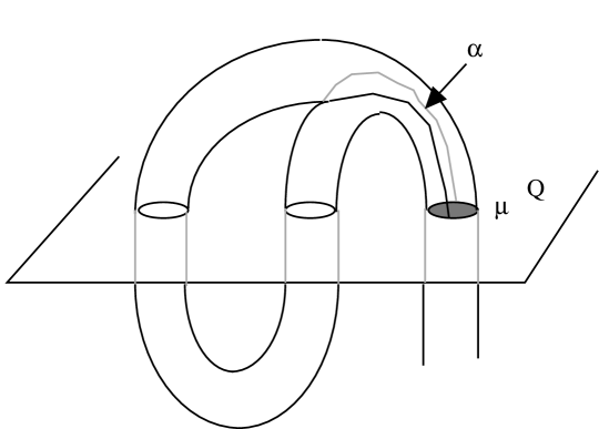
Figure 3. wave

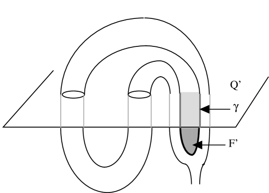
Figure 4. Splitting along a wave

Obviously $Q_{0}\cap e_{b}$ has one less point than $Q\cap e_{b}$. We claim that $Q_{0}$ is incompressible. To verify this, consider the tube dual to the compression disk (that is, $Q^{\prime}$ is recovered by tubing together two components of $Q_{0}$ along this tube). The tube is parallel to a regular arc $\gamma$ in $\mbox{$\partial$}H$ connecting the two new components of $Q_{0}$. (The regular arc is one which intersects the curve $\alpha$ in a single point.) Let $F^{\prime}$ be the disk of parallelism, so $\mbox{$\partial$}F^{\prime}$ is the union of $\gamma$ and an arc in $Q^{\prime}$ that crosses the compressing disk exactly once. If there were a further compression of $Q_{0}$ possible, it would have to fall on the same side of $Q_{0}$ as $F^{\prime}$. Then note that $F^{\prime}$ could be used to push the compressing disk off the tube. That is, the compression could have been done to $Q$, which is impossible. See Figure 5.

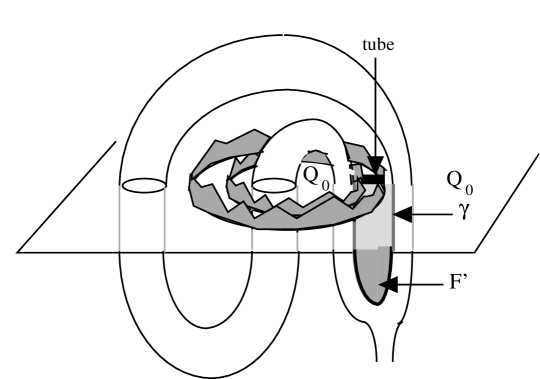
Figure 5. Tubing the spheres $Q_{0}$ to get back $Q$

So the induction hypothesis applies to $Q_{0}$. Since the first two possibilities of the lemma imply (the first case of) the third, we may as well take $F$ to be a disk as in the third possibility. Note specifically that if $Q_{0}\cap e_{b}=\emptyset$ then we can use item 1) to choose for $F$ a disk that is disjoint from $e_{b}$. When comparing the curves $\mbox{$\alpha$}=F\cap H$ and $\mbox{$\gamma$}=F^{\prime}\cap H$, we can arrange that $\mbox{$\alpha$}\cap\mbox{$\gamma$}=\emptyset$ by pushing any intersection points to the point where the tube is attached (to recover $Q^{\prime}$ from $Q_{0}$) and moving $\alpha$ across the attaching disks. Note also that at most one end of $\mbox{$\alpha$}\subset\mbox{$\partial$}F$ lies on the new meridians of $Q_{0}$ since these two meridians lie on different components of $Q_{0}$. By general position (make the tube thin) the interior of $F$ intersects $Q^{\prime}$ only in meridians of the attaching tube. Moreover, since $F$ is disjoint from $\gamma$, all intersections of $F$ with $F^{\prime}$ can be pushed via $F^{\prime}$ across the tube so that, in the end, the interior of $F$ is entirely disjoint from $Q^{\prime}$ and from $F^{\prime}$. Now use $F^{\prime}$ to $\partial$-compress $Q^{\prime}$ to recover $Q$, leaving $F$ as a disk satisfying the lemma for $Q$. ∎

We recall the definition of width for a graph; for further details see [GST]. Let $\Gamma$ be an eyeglass graph or theta graph in $S^{3}$. As in [GST], choose a height function $h$ from $S^{3}$ with two points removed to $\mathbb{R}$, and let $S(t)=h^{-}(t)$. Assume that $\Gamma$ is in Morse position with respect to $h$, that is, the critical points of $\Gamma$ with respect to $h$ occur at distinct values of $t$ and these values are distinct from the values of $h$ at the vertices of $\Gamma$. Further assume that a vertex $v$ of $\Gamma$ is either a Y-vertex (where exactly two edges of $\Gamma$ lie above $v$) or a $\lambda$-vertex (where exactly two edges of $\Gamma$ lie below $v$).

Definition 2.5.

Let $t_{0}<t_{1}<...<t_{n}$ be the successive critical heights of $\Gamma$ and suppose $t_{j}$ and $t_{k}$ are the two levels at which the vertices occur. Let $s_{i},1\leq i\leq n$ be generic levels chosen so that $t_{i-1}<s_{i}<t_{i}$. Define the width of $\Gamma$ with respect to h to be

$$W_{h}(\mbox{$\Gamma$})=2(\Sigma_{i\neq j,k}|S(s_{i})\cap(\mbox{$\Gamma$})|)+|S(s_{j})\cap(\mbox{$\Gamma$})|+|S(s_{k})\cap(\mbox{$\Gamma$})|$$

We say that $\Gamma$ is in thin position with respect to $h$ if has been isotoped to the generic position which minimizes $W_{h}$.

Figure 6. Reducing the width by $4$ via Counting Rule 1 case 4

Example 2.6.

If $\Gamma$ is a knot, then this definition of width is simply twice the width as defined by Gabai.

Example 2.7.

Suppose $e_{-}$ is a knot in $S^{3}$, in generic position with respect to $h$. Suppose $P$ is a generic level sphere that intersects $e_{-}$ in $p$ points. Construct an eyeglass graph in $S^{3}$ by attaching to $e_{-}$ the union of an edge $e_{b}$ and a loop $e_{+}$ both lying in $P$. Then when $\Gamma$ is made generic by tilting $e_{b}\cup e_{+}$,

$$W_{h}(\mbox{$\Gamma$})=W_{h}(e_{-})+4p+5.$$

Indeed, two vertices and a regular maximum (say) are added. Level spheres just below the vertices add $p$ and $p+1$ to the width. That just below the regular maximum adds $2p+4$.

We will mostly be concerned with how the width changes under isotopies of $\Gamma$, but it will be important to identify precise rules. It is simple to check the following (see Figure 6 for a sample argument):

Counting Rule 1.

1. As a maximum (either a regular maximum or a $\lambda$-vertex) is pushed below (or above) another maximum, the width does not change.

2. As a minimum (either a regular minimum or a $Y$-vertex) is pushed below (or above) another minimum, the width does not change.

3. As a regular minimum is pushed above a regular maximum, the width decreases by $8$.

4. As a regular minimum is pushed above a $\lambda$ vertex, or a regular maximum is pushed below a $Y$-vertex, the width decreases by $4$.

5. As a $Y$ vertex is pushed above a $\lambda$ vertex, or, equivalently, a $\lambda$ vertex is pushed below a $Y$-vertex, the width decreases by $2$.

6. Suppose between level spheres $P_{\pm}$ there are exactly two critical points, a regular minimum and a regular maximum on the same arc. Then replacing that arc by a vertical arc reduces the width by $4|P_{+}\cap\mbox{$\Gamma$}|+4=4|P_{-}\cap\mbox{$\Gamma$}|+4.$

Definition 2.8.

Two embeddings of a trivalent graph in $S^{3}$, both generic with respect to a height function on $S^{3}$, are width-equivalent if there is a generic isotopy from one embedding to the other so that the width is constant throughout the isotopy.

It’s obvious that any birth-death singularity during the isotopy will change the width, so the only non-generic embeddings during a width-equivalence isotopy will be ones at which two critical points are at the same level. Note that, from Counting Principle 1, the two critical points must both be maxima or both minima. In other words, if two embeddings are width-equivalent then there is an isotopy from one to the other that perhaps pushes maxima past maxima and minima past minima, but never maxima past minima.

Definition 2.9.

Suppose $\mbox{$\Gamma$}^{\prime}$ is a subgraph of a trivalent graph $\Gamma$ and $i_{1}:\mbox{$\Gamma$}\subset S^{3}$ is generic with respect to the height function $h:S^{3}\mbox{$\rightarrow$}\mathbb{R}$. We say that $\mbox{$\Gamma$}^{\prime}$ is levellable if there is an embedding $i_{2}:\mbox{$\Gamma$}\mbox{$\rightarrow$}R^{3}$ so that

• $i_{2}(\mbox{$\Gamma$}^{\prime})$ is level. That is, $hi_{2}(\mbox{$\Gamma$}^{\prime})=t,t\in\mathbb{R}$

• $i_{1}$ is width-equivalent to an embedding obtained by perturbing $i_{1}$

For example, suppose $\mbox{$\Gamma$}\subset S^{3}$ is an eyeglass graph in generic position with respect to $h$, except that one cycle $e_{\pm}$ in $\Gamma$ is level, e. g. $h(e_{+})=t$. There is a natural way to make $\Gamma$ generic, namely tilt $e_{+}$ slightly so that it is vertical, i. e. so that $e_{+}$ has a single maximum (perhaps a $\lambda$ vertex) and a single minimum (perhaps a $Y$-vertex) and one of these is the vertex of $\Gamma$ lying in $e_{+}$. The choice of whether the vertex is at the minimum or at the maximum of $e_{+}$ is determined by whether the end of the edge $e_{b}$ lies below or above the vertex. The resulting generic embedding of $\Gamma$ is one for which $e_{+}$ is levellable. In fact, using this convention, we can extend the notion of width so that it is defined when either or both of $e_{\pm}$ are level. An easy application of Counting Rule 1 shows:

Counting Rule 2.

Suppose that $e_{+}$ is level and the end of $e_{b}$ at $e_{+}$ lies below the vertex.

1. If $e_{+}$ is kept level while being moved below a regular maximum, the width increases by $4$.

2. If $e_{+}$ is kept level while being moved below a $\lambda$ vertex, the width increases by $2$.

3. If $e_{+}$ is kept level while being moved above a regular minimum, the width increases by $8$.

4. If $e_{+}$ is kept level while being moved above a $Y$ vertex, the width increases by $4$.

Of course the same rules apply when it is $e_{-}$ that is level, and symmetric rules hold if the end of $e_{b}$ at the vertex lies above the vertex. There is one final case:

Counting Rule 3.

Suppose that $e_{+}$ is level, with $h(e_{+})=t$, and the end of $e_{b}$ at $e_{+}$ lies below the vertex. Let $p=|S(t)\cap(e_{-}\cup e_{b})|$. If the end of $e_{b}$ at $e_{+}$ is moved above $e_{+}$ (introducing a new regular maximum in $e_{b}$) then the width is increased by $2p+4$.

Proof.

See Figure 7 ∎

Figure 7. Increasing $W$ by “wagging” the end of $e_{b}$

Lemma 2.10.

Let $\Gamma$ be a Heegaard spine eyeglass graph in $S^{3}$, in generic position with respect to the height function $h$. Suppose $e_{+}$ lies entirely above or entirely below $e_{-}$. Then $\Gamma$ is planar (i.e. can be isotoped to lie in a level sphere).

Proof.

The edge $e_{b}$ defines a Heegaard splitting of the reducible manifold $S^{3}-\eta(e_{+}\cup e_{-})\cong(S^{3}-\eta(e_{+})\#(S^{3}-\eta(e_{+})$. By Haken’s theorem there is some reducing sphere that intersects $e_{b}$ in a single point; planarity of $\Gamma$ (as well as the unknottedness of $e_{\pm}$) follows immediately. ∎

Lemma 2.11.

Let $\Gamma$ be the eyeglass graph described in example 2.7 and suppose $\Gamma$ is a Heegaard spine. Suppose there is a maximum of $e_{-}$ below $P$ and let $Q$ be a level sphere just above the highest such maximum. Suppose $|Q\cap\mbox{$\Gamma$}|=|Q\cap e_{-}|=q$. Then the width of $\Gamma$ can be reduced by at least $4q$.

(The symmetric statement hold if there is a minimum above $P$.)

Proof.

The proof is by induction on $q$. Let $Q^{\prime}$ be the collection of spheres obtained by maximally compressing $Q$ in the complement of $H$. Note that $Q^{\prime}$ intersects $\Gamma$ only in $e_{-}$, so Proposition 2.4 case 1 applies. The disk $F$ given by the proposition describes an isotopy that can be used to slide some part of an edge to $Q^{\prime}$. Hence, by avoiding the disks in $Q^{\prime}$ that are the results of the compressions, the edge is brought down (or up) to $Q$. The isotopy possibly passes through $Q$ on the way, but at the end $\beta$ can be taken to lie just below (resp. above) $Q$. In particular, the arc moves down past a minimum (or at least past $e_{b}\cup e_{+}$) or it moves up past a maximum. This decreases $q$ by $2$ and the width by at least $8$. This would complete the inductive step unless the arc contains the maximum just below $Q$ (which would disrupt the induction) then the arc contains at least two minima as well as that maximum. For the purposes of calculation of the resulting effect on width, we could imagine moving one of the contiguous minima up to just below the maximum (this will not thicken $\Gamma$) and then cancelling the minimum and maximum, thereby reducing the width by $4q+4$, thereby accomplishing the required reduction. ∎

For a similar but more delicate argument that will soon follow we will need to identify particularly important level spheres.

Definition 2.12.

Suppose $\mbox{$\Gamma$}\subset S^{3}$ is in generic position with respect to the height function $h$. A $Y-vertex$ at the minimum (or a $\lambda$-vertex at the maximum) of a vertical cycle is called an exceptional critical point. A generic level sphere $h^{-}(t)$ is thin if the lowest critical point above it is a minimum and the highest critical point below it is a maximum. A thin level sphere is exceptional if one (or both) of these critical points lying above or below it is exceptional.

Lemma 2.13.

Let $\Gamma$ be a Heegaard spine eyeglass graph in $S^{3}$, in generic position with respect to the height function $h$. Suppose $e_{+}$ is a vertical cycle with its minimum a $Y$-vertex $v$ and suppose that no critical height of $\Gamma$ occurs between the heights of its minimum and maximum. Suppose there is some minimum of $\Gamma$ above $e_{+}$ and $P$ is the sphere just below the lowest such minimum.

Then either $\Gamma$ is planar or the width of $\Gamma$ can be reduced by at least $2|\mbox{$\Gamma$}\cap P|$.

The symmetric statement is true for vertical cycles whose maximum is a $\lambda$-vertex.

Proof.

Special case: $e_{-}$ is disjoint from $P$.

Following Lemma 2.10 we may assume that $e_{-}$ does not lie entirely above $P$, so $e_{b}$ intersects $P$ in at least two points. The proof in this case is by induction on $|\mbox{$\Gamma$}\cap P|$, and directly mimics the proof of Lemma 2.11. Let $P^{\prime}$ be the collection of spheres obtained by maximally compressing $P$ in the complement of $H$. Since $P^{\prime}$ intersects $\Gamma$ only in $e_{b}$, Proposition 2.4 case 2 applies. The disk $F$ given by the proposition describes an isotopy that can be used to slide some part of $e_{b}$ to $P^{\prime}$. Hence, by avoiding the disks in $P^{\prime}$ that are the results of the compressions, the edge is brought down (or up) to $P$. In particular, the arc moves down past a minimum or it moves up past a maximum. This decreases $|\mbox{$\Gamma$}\cap P|$ by $2$ and the width by at least $4$. This completes the inductive step unless the arc contains the minimum just above $P$ (which would disrupt the induction). But in this case the arc contains at least two maxima as well as that minimum. For the purposes of calculation of the resulting effect on width, we could imagine moving one of the contiguous maxima down to just above the minimum (this will not thicken $\Gamma$) and then cancelling the minimum and maximum, thereby reducing the width by $4|\mbox{$\Gamma$}\cap P|+4$, via Counting Rule 1 case 6, thereby accomplishing more than the required reduction, in this case.

So henceforth we assume that $e_{-}$ intersects $P$. The structure of the argument will again mimic the proof of Lemma 2.11, though the details are a bit more complicated. Let $Q_{1},\ldots Q_{n}$, numbered from bottom to top, be the non-exceptional thin spheres for $\Gamma$. That is, just above each $Q_{i}$ is a minimum that is not the $Y$-vertex minimum of a vertical cycle, and just below each $Q_{i}$ is a maximum that is not the $\lambda$-vertex maximum of a vertical cycle. So in particular $P$ is among these spheres. Let $Q=Q_{1}\cup\ldots\cup Q_{n}$. The proof will be by induction on $\mbox{$\Gamma$}\cap Q$. Explicitly, we will show that given any counterexample, one can find a counterexample with fewer such intersection points.

Let $Q^{\prime}$ be the collection of spheres obtained by maximally compressing $Q$ in the complement of $H$. Note that $Q^{\prime}$ is disjoint from $e_{+}$. Let $F$ be the disk given by Proposition 2.4. There are two cases to consider:

Case 1: $\alpha$ is a regular arc on $\mbox{$\partial$}H$, disjoint from some meridian of $e_{b}$.

Then $F$ describes an isotopy that can be used to slide some part $e_{0}$ of an edge to $Q^{\prime}$. As usual, we can view this as bringing $e_{0}$ down (or up) to $Q$ so, at the end of the move, $e_{0}$ can be taken to lie just above (resp. below) the $Q_{i}$ to which $e_{0}$ was adjacent. In particular, the $e_{0}$ moves down past a minimum or up past a maximum. If $\mbox{$\alpha$}=\mbox{$\partial$}F\cap\mbox{$\Gamma$}$ does not go through a vertex (so $\mbox{$\alpha$}=e_{0}$), this reduces the width by at least $4$ ($8$ if the critical point it passes is not a vertex) and it reduces $\mbox{$\Gamma$}\cap Q_{i}$ by $2$. If $\alpha$ does pass through a vertex (so $e_{0}\subset\mbox{$\alpha$}$) the width drops by at least $2$ and $\mbox{$\Gamma$}\cap Q_{i}$ by $1$. Note that $\alpha$ lies between $Q_{i}$ and one of $Q_{i\pm 1}$ so, unless $P=Q_{i}$ or $Q_{i-1}$, the move can have no effect on whether $P$ remains as described, or on $\mbox{$\Gamma$}\cap P$. So unless $P=Q_{i}$ or $Q_{i-1}$ we are done, by induction. In fact, even if $P=Q_{i}$ or $Q_{i-1}$ the result of the move gives a counterexample with $Q\cap\mbox{$\Gamma$}$ reduced, so long as $P$ remains as described. That is, so long as a minimum remains just above $P$.

So suppose the slide or isotopy of $e_{0}$ to $\mbox{$\beta$}\subset Q_{i}$ removes the last minimum above $P$ and suppose first that $P=Q_{i-1}$. The effect is to remove $Q_{i-1}$ from $Q$ so the old $Q_{i}$ now serves as $P$. We compute. Let $p$ be the number of maxima between $Q_{i-1}$ and $Q_{i}$ before the move (counting any $\lambda$ vertex as $1/2$ a maximum) and let $r$ be the number of minima (counting any $Y$ vertex as $1/2$ a minimum). Then $|Q_{i-1}\cap\mbox{$\Gamma$}|-|Q_{i}\cap\mbox{$\Gamma$}|=2p-2r$. We need to show that the move just described thins $\Gamma$ by at least twice that much, plus $4$ if $\alpha$ doesn’t pass through a vertex (so $\mbox{$\Gamma$}\cap Q_{i}$ is reduced by two further points) or plus $2$ if $\alpha$ does pass through a vertex. The computation is most obvious if $\alpha$ is a single minimum with both ends on $Q_{i}$, so $r=1$ or $1/2$. Then since this minimum passes $p$ maxima the width is reduced by at least $4p$ if the minimum is regular (even if the only maximum it passes is a $\lambda$-vertex) and also $4p$ if the minimum is a $Y$-vertex, since we know that then all vertices are accounted for and the maxima are regular. In any case, we have $4p\geq 2(2p-2)+4$, completing the computation in this case.

When $\alpha$ is more complicated, containing several minima, the only difference is an even greater thinning: for computational purposes one can imagine first moving a regular minimum in $e_{0}$ above all but its contiguous maxima, then cancelling the minimum with one of those contiguous maxima. By Counting Rule 1 case 6, this already thins $\Gamma$ sufficiently; the actual isotopy would thin it even further.

The computation when $P=Q_{i}$ is similar. In this case, if the last minimum above $P$ is removed, $Q_{i+1}$ becomes the new $P$ and we need to show that the width is reduced by at least $2(|Q_{i}\cap\mbox{$\Gamma$}|-|Q_{i+1}\cap\mbox{$\Gamma$}|)$. (We do not need to add $4$ or $2$, since the move leaves $\mbox{$\Gamma$}\cap Q_{i+1}$ unchanged.) If $Q_{i}$ was the highest non-exceptional thin sphere then, for these computational purposes, substitute a sphere above $\Gamma$ for $Q_{i+1}$. Again let $p$ and $r$ be the number of maxima and minima in the relevant region, that is, between $Q_{i}$ and $Q_{i+1}$ (again, a $\lambda$ vertex or $Y$ vertex counts as only half a maximum or minimum respectively.) Since the last minimum above $P$ is being eliminated by pulling $\alpha$ down to $P$, a minimum of $\alpha$ has two contiguous maxima, which we may as well take to be the highest two maxima between the spheres. Then, for computational purposes, we can imagine eliminating that minimum first, dragging it past all but the two contiguous maxima, and then cancelling it with one of the contiguous maxima. The result is to thin by at least $4p$ (in fact $8p$ if all relevant critical points are regular) and this more than suffices.

Case 2: $\alpha$ passes exactly once through a meridian of $e_{+}$ and has its ends at the same point of $e_{b}\cap Q_{i}$.

Then $P=Q_{i}$ or $Q_{i+1}$. Suppose first that $P=Q_{i}$. Then $F$ can be used to isotope the cycle $e_{+}$ so that it lies in $Q_{i}$, but now with the end of $e_{b}$ incident to it lying above $Q_{i}$. When genericity is restored, $e_{+}$ is still vertical, but with its maximum now a $\lambda$-vertex. The simplest case to compute is when $\alpha$ runs through a single minimum of $e_{b}$, a minimum that lies just below $v$. Then the move described eliminates that regular minimum, so one less term appears in the calculation of width. This is the reverse of the operation described in Counting Rule 3, so the width is decreased by $2|Q_{i}\cap\mbox{$\Gamma$}|+4=2|P\cap\mbox{$\Gamma$}|+4$, immediately confirming the lemma. If the end of $e_{b}$ near $e_{+}$ is more complicated, the thinning is even greater.

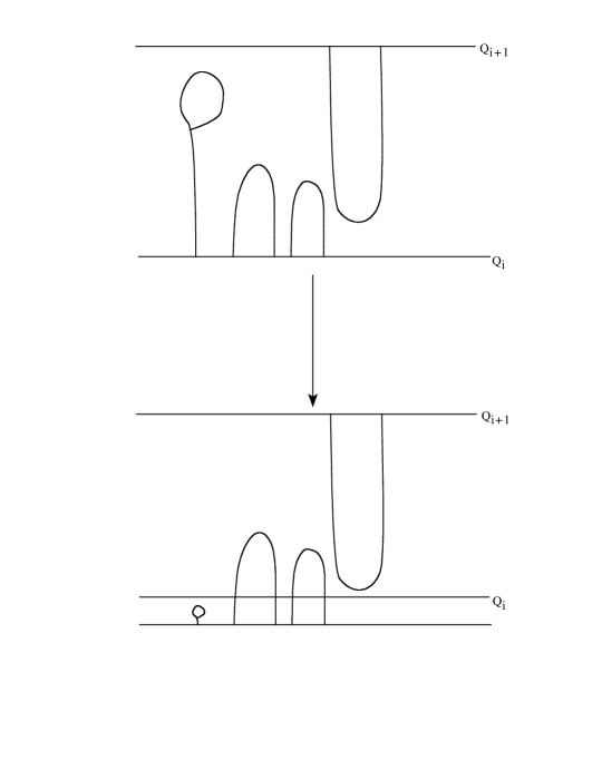
Figure 8.

Finally suppose that $P=Q_{i+1}$. In this case the isotopy given by $F$ pulls $e_{+}$ down to $Q_{i}$. Again consider the simplest case: the end segment of $e_{b}$ eliminated by the move is a simple vertical arc between $Q_{i}$ and $e_{+}$. Then $F$ pulls $e_{+}$ past $p$ maxima and $r$ minima, changing the width by $4p-8r$, essentially by Counting Rule 2. (Again a $\lambda$ vertex and $Y$ vertex count as only half a maximum or minimum respectively.) On the other hand, $|Q_{i}\cap\mbox{$\Gamma$}|$ differs from $|Q_{i+1}\cap\mbox{$\Gamma$}|$ by $2p-2r$ and $4p-8r<2(2p-2r)$. So, after the move, we have an even more extreme counterexample, and one with fewer points of intersection with $Q$. Furthermore, if $e_{b}$ is in fact more complicated than a simple vertical arc, then even more thinning would have been done. Now apply the inductive hypothesis and the contradiction completes the proof. ∎

3. Main Theorems

Theorem 3.1.

Let $\Gamma$ be a tri-valent graph that is a genus two Heegaard spine in $S^{3}$. If $\Gamma$ is in thin position then it is in extended bridge position.

Proof.

Suppose $\Gamma$ is not in extended bridge position. As previously, let $Q_{1},\ldots Q_{n}$, numbered from bottom to top, be the non-exceptional thin spheres and let $H=\eta(\mbox{$\Gamma$})$.

Suppose some $Q_{i}$ intersects $H$ only in non-separating meridians. Then the argument is much as in the Special Case of Lemma 2.13: Let $Q^{\prime}$ be the collection of spheres obtained by maximally compressing $Q_{i}$ in the complement of $H$. By Proposition 2.4 each component of $Q^{\prime}$ is parallel to a component of $\mbox{$\partial$}H-Q^{\prime}$. So in particular, there is a disk $F\subset S^{3}$ whose interior is disjoint from $H\cup Q^{\prime}$ and $\mbox{$\partial$}F=\mbox{$\alpha$}\cup\mbox{$\beta$}$, where $\mbox{$\alpha$}\subset\mbox{$\partial$}H$, $\mbox{$\beta$}\subset Q^{\prime}$ and $\alpha$ is a regular path on $\mbox{$\partial$}H$ (not intersecting some meridian of $e_{b}$, if $\Gamma$ is an eyeglass). Since $\alpha$ is disjoint from $\mbox{$\partial$}Q^{\prime}=\mbox{$\partial$}Q_{i}$, $\alpha$ lies entirely above or below, say above, the level of $Q_{i}$. Then $F$ describes an isotopy that can be used to slide some part $e_{0}$ of an edge down to $Q_{i}$. The isotopy possibly passes through $Q_{i}$ on the way, but at the end $e_{0}$ can be taken to lie just above $Q_{i}$. In particular, $e_{0}$ either lies below the minimum just above $Q_{i}$ or the arc containing that minimum has been changed to one with a single maximum just above $Q_{i}$. In any case, the graph is thinned, a contradiction.

So assume every $Q_{i}$ intersects $H$ in some separating meridians, that is, $\Gamma$ is an eyeglass graph and for each $i$, $Q_{i}\cap e_{b}\neq\emptyset$.

If any $Q_{i}$ is disjoint from both of $e_{\pm}$, we use the same argument as in the Special Case of Lemma 2.13, with $Q_{i}$ playing the role of $Q$.

So assume every $Q_{i}$ intersects either $e_{+}$ or $e_{-}$ as well as $e_{b}$. If each $e_{\pm}$ intersects some $Q_{i}$, we use the same argument as above, via Proposition 2.4 case 3. We are left with the case that $e_{+}$, say, is disjoint from all $Q_{i}$, whereas $e_{-}$ intersects every $Q_{i}$. So suppose $e_{+}$ lies between $Q_{i}$ and $Q_{i+1}$ and, for concreteness and with no loss of generality (by symmetry) assume that the point $q$ of $Q\cap e_{b}$ that is closest to $e_{+}$ lies in $Q_{i}$, some $1\leq i\leq n$. (Here if $i=n$, $Q_{i+1}$ is taken to be a level sphere above $\Gamma$.)

Claim: $e_{+}$ is a vertical cycle lying above some maximum of $\Gamma$ that lies between $Q_{i}$ and $Q_{i+1}$. The minimum of $e_{+}$ is a $Y$-vertex.

Proof of claim Let $Q^{\prime}$, as before, be the collection of spheres obtained by maximally compressing $Q_{i}$ in the complement of $H$. As we have argued, Proposition 2.4 shows that there is a disk $F$ for $Q^{\prime}$ as given in item 3b of that Proposition. That is, $\mbox{$\partial$}F$ consists of an arc $\beta$ on $Q_{i}$ with both ends at $q$ and an arc $\alpha$ on $\mbox{$\partial$}H-Q$ parallel to a cycle with both ends at $q$ and running once around $e_{+}$. $F$ can be used to pull the component of $\Gamma-Q_{i}$ that contains $e_{+}$ down to $Q_{i}$. For computational purposes we can picture this done in three stages: $e_{+}$ is replaced by a vertical cycle with its minimum (resp. maximum) at the minimum (resp. maximum) of $e_{+}$; the end of $e_{b}$ between $Q_{i}$ and $e_{+}$ is replaced by a vertical arc terminating at the minimum of $e_{+}$; and then $e_{+}$ and the end of $e_{b}$ are pulled down to $Q_{i}$. The first two steps cannot make $\Gamma$ thicker and will make it thinner unless in fact it leaves the height function on $\Gamma$ unchanged. The third move will not thicken $\Gamma$ if the original $e_{+}$ has a minimum below all the maxima (e. g. there is a regular minimum of $e_{+}$) and in fact must thin $\Gamma$ unless $e_{+}$ lies above some maximum. So, since $\Gamma$ cannot be thinned, $e_{+}$ must be a cycle containing no regular minima and lying entirely above some maximum. This proves the claim.

Having established the claim, Lemma 2.13 applied to $P=Q_{i+1}$ implies that $i=n$ so $\mbox{$\Gamma$}\cap P=\emptyset$. But even then, the argument of Lemma 2.13 still suffices to display the same contradiction: The effect of pulling $e_{+}$ to $Q_{i}$ is to alter the width by adding at most $4p-8r$. On the other hand, after the move, $Q_{i}$ is then suitable (when pushed just above $e_{+}$) for applying Lemma 2.13. (See Figure 8.) This lemma says that $\Gamma$ can be thinned by $2|Q_{i}\cap\mbox{$\Gamma$}|=4p-4r>4p-8r$. ∎

Definition 3.2.

Suppose $\Gamma$ is in bridge position. Then a level sphere separating the minima from the maxima is called a dividing sphere for $\Gamma$.

If $\Gamma$ is not in bridge position, but is in extended bridge position, then a dividing sphere is a level sphere $P$ for which every minimum above $P$ is the $Y$-vertex of a vertical cycle and every maximum below $P$ is the $\lambda$-vertex of a vertical cycle.

Theorem 3.3.

Let $\Gamma$ be a tri-valent graph that is a genus two Heegaard spine in $S^{3}$. If $\Gamma$ is in thin position then it is in extended bridge position. Either $\Gamma$ is planar or some dividing sphere is disjoint from a simple (i. e. non-loop) edge of $\Gamma$.

Proof.

Following Theorem 3.1 we can assume that $\Gamma$ is in extended bridge position. If $\Gamma$ is in (non-extended) bridge position, the proof (and Corollary 3.4) will conclude much as in Theorems [GST, 5.3, 5.14]. We note that were we content to find either a level edge or an unknotted cycle in $\Gamma$, we would be done following this case. However the pursuit of a simple edge requires more persistence. Since the delicate points in the argument will need to be repeated in the case of extended bridge position we only summarize the proof when $\Gamma$ is in bridge position:

There is a dividing sphere $Q$ between the lowest maximum and the highest minimum that cuts off both an upper disk and a lower disk. If an edge running between distinct vertices lies above or below $Q$ we are done. So we can assume that each component of $\mbox{$\Gamma$}-Q$ is either an arc or a $3$-prong. (This fact makes some of the complications in the proof of [GST, 5.3] irrelevant.) There is an argument to show that we can find such upper and lower disks so that their interiors are disjoint from $Q$ and that neither intersects $Q$ in a loop. Each is incident to exactly two points of $\mbox{$\Gamma$}\cap Q$ and it is shown that at least one point, and perhaps both, are the same for both upper and lower disks.

If both upper and lower disks are incident to the same pair of points, then these disks can be used to make a cycle (either a loop or a $2$-cycle) level. The argument of [GST, 5.14] shows that if the cycle is a loop then either $\Gamma$ could be thinned (a contradiction to hypothesis) or $e_{b}$ is already disjoint from the dividing sphere and we are done. Essentially the same argument applies in the case of a level $2$-cycle, unless the third edge too can be moved into the sphere. In the latter case, the graph is planar.

If the upper and lower disks are incident to only one point of $\mbox{$\Gamma$}\cap Q$ in common, then they may be used either to thin $\Gamma$ or to make that edge level, lying in $Q$. In this case, too, $\Gamma$ may be thinned, or another edge brought to $Q$ (creating a level $2$-cycle) this time by using an outermost disk of a meridian $E$ for $S^{3}-H$, cut off of $E$ by $Q-H$. For details see [GST, 6.1, Subcases 3a, 3b].

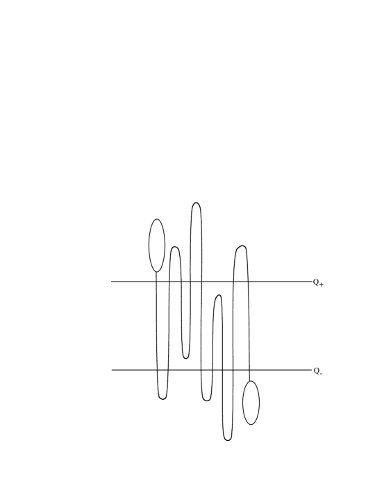
Figure 9.

So now assume that $\Gamma$ is not in bridge position, but only in extended bridge position. In particular, all thin spheres are exceptional and there is at least one exceptional thin sphere.

Claim 1: There is exactly one exceptional thin sphere and it intersects exactly one of the loops $e_{\pm}$.

Proof of Claim 1: Since there are at most two vertical cycles, there are at most two exceptional thin spheres. If there are two, denote them by $Q_{\pm}$, with $Q_{+}$ lying above $Q_{-}$ (Figure 9). Consider the lowest minimum above $Q_{+}$ and the highest maximum below $Q_{-}$. It can’t be that neither of these critical point is exceptional, for then $\Gamma$ would not be in extended bridge position. If both critical points are exceptional, then $\Gamma$ is planar by Lemma 2.10. So we may as well assume that both exceptional vertices are exceptional minima, one just above $Q_{-}$ and one just above $Q_{+}$. But then $Q_{-}$ intersects $\Gamma$ only in $e_{b}$, contradicting thin position, via Proposition 2.4 case 2.

Having established that there is exactly one exceptional thin sphere, the same argument shows that it cannot be disjoint from both $e_{\pm}$.

With no loss of generality, suppose $e_{+}$ but not $e_{-}$ is disjoint from the exceptional thin sphere $Q$.

Claim 2: The loop $e_{+}$ can be isotoped to lie in $Q$, without increasing the width of $\Gamma$.

Proof of Claim 2: Maximally compress the exceptional level sphere $Q$ in the complement of $H$ and call the result $Q^{\prime}$. Apply Lemma 2.4 to deduce that there is a disk $F$ as in item 3. Since it cannot describe a way to slide an edge segment of $\mbox{$\Gamma$}-Q$ to the level of $Q$ (that would make $\Gamma$ thinner), $\mbox{$\partial$}(F)$ must be disjoint from $e_{-}$ and run around $e_{+}$. $F$ can then be used to isotop $e_{+}$, as required. Since the vertex of the loop is immediately adjacent to $Q$, this does not thicken $\Gamma$.

Following the isotopy of Claim 2, $e_{+}$ divides $Q$ into two disks, $Q_{1}$ and $Q_{2}$. Consider the intersection of these $Q_{i}$ with a meridian disk $E$ of $S^{3}-H$. Note that there can be no closed components of intersection, since an innermost one, if essential in $Q_{i}-\mbox{$\Gamma$}$, could be used to push part of $\Gamma$ through $Q_{i}$, thinning $\Gamma$. (It is thinned, per Counting Rule 2, because an upper cap would contain no minima, and a lower cap would contain more minima than maxima). Similarly, an outermost arc of $E-Q_{i}$ can’t cut off a disk lying entirely above $Q$, for it could be used to thin and, indeed, unless $Q$ and $e_{b}$ are disjoint, so could a lower one, essentially by Counting Rule 3 applied in reverse.

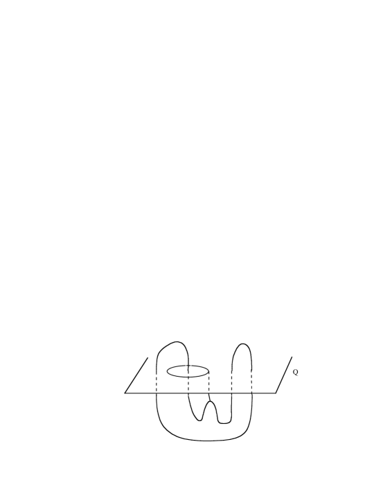
Figure 10.

So we may as well assume that $e_{b}\cap Q=\emptyset$. We know that a maximum lies just below $Q$. One possibility is that there is a regular maximum below $Q$. Another is that the only maximum below $Q$ is a $\lambda$-vertex (Figure 10).

In the second case, if the end of $e_{b}$ is incident to the $\lambda$-vertex from above, then $e_{b}$ is monotonic (for otherwise an internal maximum would lie below $Q$ or $e_{b}$ would intersect $Q$, both possibilities we are not considering). Then $e_{b}$ is disjoint from the level sphere (a dividing sphere) just below the $\lambda$-vertex, and we are done. So either there is a regular maximum below $Q$ or the $\lambda$-vertex below $Q$ has the end of $e_{b}$ incident to the vertex from below. In particular, a level sphere just below either sort of maximum would cut off an upper disk. So, as is now standard, some dividing sphere $P$ can be placed so that it simultaneously cuts off both an upper disk $D_{u}$ and a lower disk $D_{l}$. As noted above, we can assume that neither disk has a closed curve of intersection with $Q$. We now proceed to duplicate, in this context, the proof of [GST, 5.3]. The added difficulties here are apparent even at the first step. We will consider the intersections of the interiors of $D_{u}$ and $D_{l}$ with $P$.

Claim 3: (cf. [GST, Claim 5.5]) There cannot be both an upper cap and a lower cap whose boundaries are disjoint.

Proof of Claim 3: Let $C_{u}$ and $C_{l}$ denote the caps. They bound disjoint disks $P_{u}$ and $P_{l}$ in $P$. If the end segment of $e_{b}$ at $e_{+}$ is not incident to $P_{u}$ the proof is natural: pushing $C_{u}$ down to $P_{u}$ and $C_{l}$ up to $P_{l}$ will thin $\Gamma$. So assume that $e_{+}$ does lie between $C_{u}$ and $P_{u}$. If any maximum is incident to $P_{u}$ and is lower than the height of $Q$ (i. e. the height of $e_{+}$) then $\Gamma$ could be thinned by just pushing that maximum down while pushing $C_{l}$ up. So any maximum lying between $C_{u}$ and $P_{u}$ is higher than $e_{+}$. On the other hand, if any maximum not between $C_{u}$ and $P_{u}$ were above $e_{+}$ it could be pushed lower (since its easy to make the descending disk from that maximum disjoint from $C_{u}$. This too would thin $\Gamma$. Hence we see that the $p\geq 0$ maxima that are lower than $e_{+}$ are precisely those that don’t lie between $C_{u}$ and $P_{u}$.

Now consider the effect of pushing $C_{u}$ down to $P_{u}$ while simultaneously pushing $C_{l}$ up to $P_{l}$. Apply Counting Rule 2: Pushing $e_{+}$ past $p$ maxima increases the width by $4p$ whereas pushing up the $r\geq 1$ minima between $C_{l}$ and $P_{l}$ reduces the width by $8r$. (Here, as was usual in such counting above, a $\lambda$-vertex or $Y$ vertex counts as only half a maximum or minimum). The result is that, after the push, the width is increased by at most $4p-8r$. On the other hand, after the push, $P$ would satisfy the hypotheses of Lemma 2.13. It’s easy to calculate $P\cap\mbox{$\Gamma$}$: it’s $2p-2r$. Then according to that lemma, $\Gamma$ could be thinned by a further $4p-4r>4p-8r$, a contradiction establishing the claim.

Claim 4: (cf. [GST, Claim 5.6]) If there is an upper disk and a disjoint lower cap, then we can find such a pair for which the interior of the upper disk is disjoint from $P$. (The symmetric statement is of course also true.)

Proof of Claim 4: Let $B_{u}$ and $B_{l}$ denote the balls above and below the dividing sphere $P$ respectively. The proof would follow just as in [GST] if we could find a complete collection $\Delta$ of descending disks for $\mbox{$\Gamma$}\cap B_{u}$ such that the boundaries of $\Delta$ and $D_{u}$ intersect only on $P$. We do not need to worry here, as we did there, about components of $\mbox{$\Gamma$}\cap B_{u}$ that contain two vertices for if such a component exists the lemma is proven. What we do need to worry about is that any maxima that are higher than the loop $e_{+}$ have no descending disks at all (or rather, their descending disks encounter $e_{+}$ at $Q$ and do not descend to $P$, else we could thin $\Gamma$.) But because we have established above that $D_{u}$ is disjoint from $Q$ there is an easy fix. The graph $\Gamma$ intersects the region $S_{P}^{Q}\cong S^{2}\times I$ between $Q$ and $P$ in a collection of maxima and a collection of vertical arcs. At the top of one vertical arc $\epsilon_{b}$ (an end of $e_{b}$) we see the bottom half of the loop $e_{+}$. Let $T$ be the union of two trees in $Q-e_{+}$, each having a root at the vertex in $e_{+}$, each on opposite sides of $e_{+}$ and together containing all the other points of $\mbox{$\Gamma$}\cap Q$. (These points are just the tops of the vertical arcs of $\mbox{$\Gamma$}\cap S_{P}^{Q}$.) Denote the edges of $T$ by $E_{T}$. Finally, let $C\subset S_{P}^{Q}$ be the vertical cylinder $e_{+}\times I$, intersecting $\Gamma$ exactly in $\epsilon_{b}\cup e_{+}$. Define $\Delta$ to be this collection of disks: $\{E_{T}\}\times I$, $C-\eta(\epsilon_{b})$, and a set of descending disks for all maxima in $S_{P}^{Q}$, these chosen to be disjoint from the other disks in $\Delta$. Clearly $\Delta$ cuts $S_{P}^{Q}$ up into a collection of balls. See Figure 11.

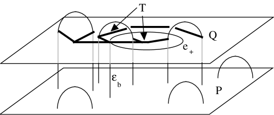
Figure 11.

Now observe that $D_{u}$ cannot involve the maxima that are higher than $Q$, else $\Gamma$ could be thinned. Hence the part of the boundary of $D_{u}$ that lies on $\Gamma$ either lies on a maximum in $S_{P}^{Q}$ or on the component containing $e_{+}$. In either case it is easily made disjoint from $\partial$$\Delta$ so that $\mbox{$\partial$}D_{u}\cap\mbox{$\partial$}\mbox{$\Delta$}$ lies entirely in $P$. The proof now follows as in [GST, Claim 5.6].

With one exception, the proof of Theorem 3.3 is now little different from the flow of the proof of [GST, Theorem 5.3]: ultimately we get upper and lower disks which can be used to push part of $\mbox{$\Gamma$}\cap B_{l}$ up while pushing part of $\mbox{$\Gamma$}\cap B_{u}$ down. Unless the latter is the component containing $e_{+}$, this immediately thins $\Gamma$. So suppose $D_{u}$ does push down $e_{+}$; let $p$ denote the point in $e_{b}$ where that component is cut off. Unless $D_{l}$ pushes up a segment incident to $p$, the proof follows by a width count and Lemma 2.13 just as in the proof of Claim 3. If the segment incident to $p$ that $D_{l}$ pushes up is a simple minimum (i. e. it does not contain the other end of $e_{b}$) then that push eliminates a critical point which we may take to lie just below $P$. In particular, for $P_{+}$ a level sphere just above $P$, the move reduces the width by $2|\mbox{$\Gamma$}\cap P_{+}|+4$ via Counting Rule 2, and this is enough again to ensure that after the move the graph is thinner.

Finally, suppose that $D_{l}$ is incident to $p$ and pushes up the other end of $e_{b}$. (This implies in particular that $e_{b}\cap P=\{p\}$.) Then after the move both the edges $e_{b}\cup e_{+}$ are level and lie in $P$. But, as usual, the move may thicken $\Gamma$ and this time there is no immediate cancellation of a critical point since $e_{b}$ was monotonic before the move, just as it would be again when genericity is restored. The thickening occurs, as usual, because the $Y$-vertex minimum of $e_{+}$ may be pulled down past $m$ maxima, in which case the width increases by $4m$. But, unless $m=0$, this leads to a contradiction: Consider the cylinder $C$ that is swept out by $e_{+}$ as it is pulled down to $P$ (effectively, this is just another way of viewing the upper disk $D_{u}$) and apply the technical Lemma 4.1 that follows. The resulting graph could in fact be thinned by a further $4m+4$, leaving it thinner than we started. So we conclude that $m=0$ and the move can be made without any thickening at all.

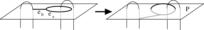
Figure 12. Tilting $e_{b}\cup e_{+}$

Once $e_{b}\cup e_{+}$ is level, tilt it slightly, creating two $Y$-vertices, say, one at each end of $e_{b}$, so $e_{+}$ is vertical with its maximum a regular maximum. Then a level sphere passing through the middle of $e_{+}$ is a dividing sphere that is disjoint from $e_{b}$, as required. See Figure 12. ∎

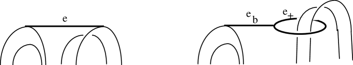
Figure 13. Levellable edge or subgraph

Corollary 3.4.

Let $\Gamma$ be a tri-valent graph that is a Heegaard spine in $S^{3}$ and suppose that $\Gamma$ is in thin position. Then at least one simple edge is levellable (cf Definition 2.9). To be specific, either $\Gamma$ is planar or (see Figure 13):

1. If $\Gamma$ is in bridge position then there is a simple edge $e\subset\mbox{$\Gamma$}$ so that

   • the knot or link $K=\mbox{$\Gamma$}-interior(e)$ is in bridge position and

   • $e$ is levellable and its ends lie at distinct maxima or at distinct minima of $K$

2. If $\Gamma$ is not in bridge position then $\Gamma$ is an eyeglass graph. For some loop (say $e_{-}$) in $\Gamma$

   • $e_{-}$ is in bridge position and

   • the subgraph $e_{b}\cup e_{+}$ is levellable and is incident to either a maximum or minimum of $e_{-}$.

Proof.

We assume $\Gamma$ is not planar and first suppose $\Gamma$ is in bridge position. Let $P$ be a dividing sphere disjoint from a non-loop edge $e$ of $\Gamma$ guaranteed by Theorem 3.3. With no loss of generality the edge $e$ lies above $P$. Let $\mbox{$\Gamma$}_{u}$ denote the part of $\Gamma$ lying above $P$. Since there are no minima above $P$, a family of descending disks for $\mbox{$\Gamma$}_{u}$ describes a parallelism between $\mbox{$\Gamma$}_{u}$ and a subgraph of $P$. In particular, $e$ can be viewed as a perturbed level edge.

Suppose next that $\Gamma$ is not in bridge position. We know from Theorem 3.1 that $\Gamma$ is extended bridge position so in particular $\Gamma$ is an eyeglass graph. Let $P$ be a dividing sphere disjoint from the edge $e_{b}$, as guaranteed by Theorem 3.3. We may as well assume $e_{b}$ lies above $P$, so one end of $e_{b}$ descends from the minimum of a vertical loop, say $e_{+}$. Since $e_{b}$ is disjoint from the dividing sphere $P$ it contains no minimum and its other end ascends from a $\lambda$-vertex, hence from a maximum of $e_{-}$. Raise that maximum along $e_{b}$ until it is the critical point just below the $Y$-vertex. Let $Q$ be a level plane that intersects the monotonic edge $e_{b}$ in a single point. Maximally compress $Q$ in the complement of $\Gamma$ and let the result be $Q^{\prime}$. As has been argued repeatedly above, if we apply Proposition 2.4 to $Q^{\prime}$ the only conclusion that does not violate thinness is possibility 3.b. In that case, the disk $F$ describes how to isotope $e_{b}\cup e_{+}$ to lie in $P$. Since there are no critical points between the heights of the ends of $e_{b}$ this has no effect on width. ∎

4. Technical Lemma

For the following technical lemma we return to the context of Example 2.7 and Lemma 2.11. That is, $e_{-}$ is generic with respect to a height function on $S^{3}$ and the subgraph $e_{b}\cup e_{+}$ is level with respect to the height function, at a height that is generic for $e_{-}$. Width is calculated by tilting $e_{b}\cup e_{+}$ slightly to restore genericity. This is independent of the direction of tilting.

Lemma 4.1.

Suppose $\Gamma$ is a non-planar eyeglass graph that is a Heegaard spine of $S^{3}$. Suppose there is a height function on $S^{3}$ and a dividing sphere $P$ for $e_{-}$ that contains both the edges $e_{b}$ and $e_{+}$. Suppose $Q$ is a level sphere above $P$ and there is a properly embedded annulus $C$ such that

1. $C$ spans the region $S_{P}^{Q}\cong S^{2}\times I$ that lies between $Q$ and $P$

2. $\mbox{$\partial$}C\cap P=e_{+}$ and

3. $C\cap\mbox{$\Gamma$}=e_{+}$.

Let $m>0$ be the number of maxima of $e_{-}$ in $S_{P}^{Q}$. Then $\Gamma$ can be isotoped so that $e_{b}\cup e_{+}$ is again level, but the width of $\Gamma$ has been reduced by at least $4m+4$.

Proof.

The cycle $e_{+}$ divides $P$ into two disks $P_{1}\cup P_{2}$. Without loss of generality, assume that $e_{b}$ lies in $P_{2}$. Let $S_{P,i}^{Q},i=1,2$ denote the component of $S_{P}^{Q}$ lying above $P_{i}$.

Case 1: Some maximum (resp. minimum) of $e_{-}$ can be pushed down (resp. up) past $P$.

Note that a plane just above or below $P$ intersects $e_{-}$ in at least $2m$ points. If the maximum that is pushed down is not the maximum contiguous to the end of $e_{b}$ then the move instantly reduces the width of $\Gamma$ by $8$, per 2.7. More importantly, after the move $\Gamma$ is in a position to apply Lemma 2.11, and so we can reduce the width by at least a further $4(2m-2)$. Thus the total width is reduced by at least $8m\geq 4m+4$.

If the maximum that is pushed down is contiguous to the end of $e_{b}$, the effect on width is to first push a regular maximum down past a $Y$-vertex (on $e_{+}$) and then to convert the regular maximum and the $Y$-vertex on $e_{-}$ into a single $\lambda$ vertex on $e_{-}$. The first move reduces the width by $4$ and the second move (eliminating a critical point) reduces it by at least a further $4m+2$.

Case 2: Some maximum of $e_{-}$ lies in $S_{P,1}^{Q}$.

The descending disk of any maximum in this region can’t intersect the end $C\cap Q$, since that end is too high. Hence the intersection of such a descending disk with $C$ consists entirely of components that are inessential in $C$. It follows that a disk in $S_{P,1}^{Q}$ can be found that isotopes a maximum of $e_{-}$ in $S_{P,1}^{Q}$ down to a level below $P$, returning us to Case 1.

Let $H$ be a regular neighborhood of $\Gamma$ and continue to call $P_{i}$ the disks obtained by removing the boundary collars given by $H\cap P_{i}$. Then each $P_{i}$ is a disk punctured by meridians of $H$ associated with points on $e_{-}$. Since $P$ was a dividing sphere for $e_{-}$, there are an odd number $p$ of such meridians (the point of $e_{-}$ at the end of $e_{b}$ does not, of course, give rise to such a meridian). $P$ divides $\mbox{$\partial$}H$ into $p+1$ components; $p-1$ of them are annuli $A_{1},\ldots,A_{p-1}$ lying between meridian disks associated to points in $e_{-}\cap P$. Two components, $U_{\pm}$ are pairs of pants, with boundary of each consisting of $\mbox{$\partial$}P_{1},\mbox{$\partial$}P_{2}$ and the boundary of a meridian associated to a point of $e_{-}\cap P$. Choose notation so that $U_{+}$ lies above $P$, the meridian curves in $\mbox{$\partial$}H$ associated to points of $e_{-}\cap P$ occur in order $\mu_{1},\ldots,\mu_{p}$ along $e_{-}$, with $\mu_{1}\subset\mbox{$\partial$}U_{+}$ and $\mu_{p}\subset\mbox{$\partial$}U_{-}$ and, finally, $\mbox{$\partial$}A_{i}=\mu_{i}\cup\mu_{i+1}$.

Not surprisingly, we consider how a meridian disk $E$ of $S^{3}-H$ intersects $P$. It will eventually be useful to have chosen $E$, among all possible meridian disks, to minimize $|E\cap P|$. Of course if $E$ is disjoint from $P$ then its boundary can’t be a meridian curve of $e_{-}$ (every sphere in $S^{3}$ separates) so it must be parallel to $\mbox{$\partial$}P_{1}$. But then it’s easy to see that $\Gamma$ is in fact planar, contradicting hypothesis. If there are any closed components of $E\cap(P_{1}\cup P_{2})$ then an innermost one on $E$ can be used to push a maximum below $P$ or a minimum above $P$. Then we are in Case 1 and the argument is complete. A similar argument applies if an outermost disk $E_{0}$ cut off from $E$ by $P_{i}$ is incident to one of the $A_{i}$. We conclude that $E\cap P$ consists entirely of arcs and, furthermore, each outermost disk is incident only to one of $U_{\pm}$. Let $E_{0}$ be any such outermost disk, with boundary the union of two arcs $\mbox{$\alpha$}\subset\mbox{$\partial$}\eta(H)\cap E$ and $\mbox{$\beta$}\subset P\cap E$ in $E$. Consider the possibilities for $\alpha$.

Case 3: One or both ends of $\alpha$ is incident to $\mbox{$\partial$}P_{2}$.

The other end of $\alpha$ can’t be incident to $\mbox{$\partial$}P_{1}$, for the arc $\mbox{$\beta$}=E_{0}\cap P$ lies either in $P_{1}$ or $P_{2}$. If the other end is incident to $\mu_{1}$ then it can be used to pull the maximum of $e_{-}$ contiguous to the end of $e_{b}$ down below $P$, again placing us in Case 1. Similarly if the other end of $\alpha$ is incident to $\mu_{p}$. In fact, if both ends of $\alpha$ lie on $\mbox{$\partial$}P_{2}$ we can accomplish the same thing, essentially using $E_{0}$ much like a cap.

Case 4: Exactly one end of $\alpha$ is incident to $\mbox{$\partial$}P_{1}$.

Again, the other end of $\alpha$ can’t be incident to $\mbox{$\partial$}P_{2}$. Suppose it is incident to $\mu_{p}$. Then, since an arc in a pair of pants is determined up to proper isotopy by its end points, the arc $\alpha$ runs once along the length of $e_{b}$, then over the minimum of $e_{-}$ that is adjacent to the end of $e_{b}$ and ends in $\mu_{p}\subset P_{1}$. The disk $E_{0}$ can be used to slide $e_{b}$, keeping the end at $e_{+}$ fixed, until $e_{b}$ becomes the arc $\mbox{$\beta$}\subset P_{1}$. See Figure 14. Afterwards, the width is unaffected, but all $m$ maxima now lie in the component $S_{P,2}^{Q}$ that no longer contains $e_{b}$. In effect, we are in Case 2 and so we are finished once again. The same argument applies if the other end of $\alpha$ is at $\mu_{1}$: Since the interior of $E_{0}$ is disjoint from $\Gamma$ the slide of $e_{b}$ to $\beta$ has no effect on the maxima in $S_{P,2}^{Q}$, or on the cylinder $C$. (The edge $e_{b}$ just passes through $C$).

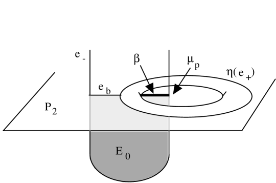
Figure 14. Case 4

Case 5: Both ends of $\alpha$ are incident to $\mbox{$\partial$}P_{1}$.

Suppose, to be concrete, that $E_{0}$ lies above $P$, so it forms a kind of cap or shroud over the part $e_{0}$ of $e_{-}$ that lies between $e_{b}$ and $\mu_{1}$. Let $A$ denote the annulus half of $\mbox{$\partial$}\eta(e_{b}\cup e_{+})$ that lies above $P$ and let $P_{u}$ denote the plane $P_{1}\cup A\cup P_{2}$. Then $\mbox{$\partial$}E_{0}\subset P_{u}$ consists of two arcs, $\mbox{$\alpha$}\subset A$ and $\mbox{$\beta$}\subset P_{1}$. A descending disk for the maximum $e_{0}$ also has boundary consisting of two arcs, one being $e_{0}$ itself and the other an arc in $P_{u}$. A standard innermost disk, outermost arc argument shows that such a disk $D$ can be found disjoint from $E_{0}$, so $\mbox{$\partial$}D$ lies in the disk in $P_{u}$ bounded by $\mbox{$\partial$}E_{0}$. In fact, $E_{0}$ can be used to remove (by piping to $E_{0}$ and then over it) any arc of $\mbox{$\partial$}D\cap A$ which is parallel to $\alpha$ in the punctured annulus $A-e_{0}$. The upshot is that, if we choose $D$ so that the arc $\mbox{$\delta$}=\mbox{$\partial$}D\cap P_{u}$ intersects $A$ in a minimal number of components, then in fact $\delta$ consists of a single arc in $A$ (running from the end of $e_{0}$ to $\mbox{$\partial$}P_{1}$) and a single arc in $P_{1}$. Once this is accomplished, the disk $D$ can be used instead of $E_{0}$ in the proof of Case 4, completing the argument in this case.

Case 6: The general case.

Following cases 3 to 6, the only remaining case to consider is one in which every outermost arc cut off by $P_{1}\cup P_{2}$ has both ends incident to $\mu_{1}$ (when the disk it cuts off lies above $P$) or both ends incident to $\mu_{p}$ (when the disk it cuts off lies below $P$). Notice that, in either case, the outermost arc forms a loop in $P$ with both ends either at $\mu_{1}$ or at $\mu_{p}$.

Claim: For any $\mu_{i},1\leq i\leq p$, there is an arc of $E\cap P$ forming a loop at $\mu_{i}$.

The proof of the claim is a particularly easy application of outermost forks. Cf [Sc] for details beyond this sketch: Label the ends of arcs of $P\cap E$ in $\mbox{$\partial$}E$ that lie on the meridians $\mu_{1},\ldots,\mu_{p}$ by the number of the corresponding meridian. We have just demonstrated that each outermost arc has either both ends labelled $1$ or both ends labelled $p$. To the collection of arcs $E\cap P$ there is naturally associated a tree in $E$, with a vertex in each component of $E-P$ and an edge connecting any vertices corresponding to adjacent components. Consider an outermost fork of this tree. Two adjacent tines of this fork have ends labelled $(1,1)$ or $(p,p)$. In order to get from one labelling to the other, the arc of $\mbox{$\partial$}E$ that lies between the ends of the two adjacent tines must go sequentially through every label from $1$ to $p$ (perhaps more than once). Since each arc of $E\cap P$ it passes by is parallel to an outermost arc, its labels must be the same. The result is a collection of arcs containing all labels $1,\ldots,p$ and having the same label at each end. (See Figure 15). These arcs, when considered in $P$, form loops at every meridian $\mu_{p}$.

Figure 15.

Having established the claim, consider this consequence: An innermost such loop contains no meridian in its interior. This means that an innermost loop can be used to $\partial$-compress $E$ to $\mbox{$\partial$}H$, dividing $E$ into two disks, at least one of which is still a meridian disk and each of which intersects $P$ in fewer arcs. Since $E$ was initially chosen to minimize $E\cap P$, this is impossible. ∎

References

- [GST] H. Goda, M. Scharlemann and A. Thompson, Levelling an unknotting tunnel, Geometry and Topology 4 (2000) 243–275.
- [GR] C. Gordon and A. Reid, Tangle decompositions of tunnel number one knots and links, J. Knot Rami. 4 (1995) 389-409.
- [Mo] K. Morimoto, Planar surfaces in a handlebody and a theorem of Gordon-Reid, Proc. Knots ’96, ed.S.Suzuki, World Sci.Publ.Co.,Singapore (1997), 127-146.
- [Sc] M. Scharlemann Outermost forks and a theorem of Jaco, Combinatorial methods in topology and algebraic geometry (Rochester 1982), Contemp. Math. 44 (1985) 189-193.
- [ST1] M. Scharlemann and A. Thompson Heegaard splittings of (surface) are standard Math. Ann. 295 (1993) 549-564.
- [ST2] M. Scharlemann and A. Thompson Thin position and Heegaard splittings of the 3- sphere Jour. Diff. Geom. 39 (1994) 343-357.
- [Wa] F. Waldhausen, Heegaard-Zerlegungen der 3-Sphäre, Topology, 7 (1968), 195-203.