Inverse spectral problem for analytic domains II:
${\mathbb{Z}}_{2}$- symmetric domains

Abstract.

This paper develops and implements a new algorithm for calculating wave trace invariants of a bounded plane domain around a periodic billiard orbit. The algorithm is based on a new expression for the localized wave trace as a special multiple oscillatory integral over the boundary, and on a Feynman diagrammatic analysis of the stationary phase expansion of the oscillatory integral. The algorithm is particularly effective for Euclidean plane domains possessing a ${\mathbb{Z}}_{2}$ symmetry which reverses the orientation of a bouncing ball orbit. It is also very effective for domains with dihedral symmetries. For simply connected analytic Euclidean plane domains in either symmetry class, we prove that the domain is determined within the class by either its Dirichlet or Neumann spectrum. This improves and generalizes the best prior inverse result (cf. [Z1, Z2, ISZ]) that simply connected analytic plane domains with two symmetries are spectrally determined within that class.

1. Introduction

This paper is part of a series (cf. [Z5, Z4]) devoted to the inverse spectral problem for simply connected analytic Euclidean plane domains $\Omega$. The motivating problem is whether generic analytic Euclidean drumheads are determined by their spectra. All known counterexamples to the question, ‘can you hear the shape of a drum?’, are plane domains with corners [GWW1], so it is possible, according to current knowledge, that analytic drumheads are spectrally determined. Our main results give the strongest evidence to date for this conjecture by proving it for two classes of analytic drumheads: (i) those with an up/down symmetry, and (ii) those with a dihedral symmetry. This improves and generalize the best prior results that simply connected analytic domains with the symmetries of an ellipse and a bouncing ball orbit of prescribed length $L$ are spectrally determined within this class [Z1, Z2, ISZ].

The proofs of the inverse results involve three new ingredients. The first is a simple and precise expression (cf. Theorem 3.1) for the localized trace of the wave group (or dually the resolvent), up to a given order of singularity, as a finite sum of special oscillatory integrals over the boundary $\partial\Omega$ of the domain with transparent dependence on the boundary defining function. Theorem 3.1 is a general result combining the Balian-Bloch approach to the wave trace expansion of [Z5] with a reduction to boundary integral operators explained in [Z4]. Presumably it could be obtained by other methods, such as the monodromy operator method of Iantchenko, Sjöstrand and Zworski [SZ, ISZ]. Aside from this initial step, this paper is self-contained.

The next and most substantial ingredient is a stationary phase analysis of the special oscillatory integrals in Theorem 3.1. To bring order into the profusion of terms in the wave trace (or resolvent trace) expansion, we use a Feynman diagrammatic method to enumerate the terms in the expansion. Diagrammatic analyses have been previously used in [AG] (see also [Bu]) to compute the sub-principal wave invariant. A novel aspect of the diagrammatic analysis in this paper is its focus on the diagrams whose amplitudes involve the maximum number of derivatives of the boundary in a given order of wave invariant. A key result, Theorem 4.2, is that only one term, the principal term in Theorem 3.1, contributes such highest derivative terms. That is, the stationary phase expansion of the principal term generates all terms of the $j$th order wave invariant (for all $j$) which depend on the maximal number $2j-2$ of derivatives of the curvature of the boundary at the reflection points. In the principal term, the ‘transparent dependence’ of the phase and amplitude on the boundary is encapsulated in the simple properties of the phase and amplitude stated in the display in Theorem 4.2. Only these properties are used to make the key calculations of the wave invariants stated in Theorem 5.1.

This focus on highest derivative terms in each wave invariant turns out to be crucial for the inverse spectral problem on domains with the symmetries studied in this article. The third key ingredient is the analysis in §6 of these highest order derivative terms in the case of domains in our two symmetry classes. The main result is that the other terms in the wave invariants are redundant, and further that the domain can be determined from the wave invariants within these symmetry classes. These results are based on the use of the finite Fourier transform to diagonalize the Hessian matrix of the length function, and an analysis of Hessian power sums.

As this outline suggests, we take a direct approach to calculating wave trace invariants and do not employ Birkhoff normal forms as in [G, Z1, Z2, Z3, ISZ]. We do this because the classical normal form of the first return map does not contain sufficient information to determine domains with only one symmetry. Therefore one would need to use the full quantum Birkhoff normal form. But we found the calculations based on the Balian-Bloch approach simpler than those involved in the full quantum Birkhoff normal form.

1.1. Statement of results

Let us now state the results more precisely. We recall that the inverse spectral problem for plane domains is to determine a domain $\Omega$ as much as possible from the spectrum of its Euclidean Laplacian $\Delta^{\Omega}_{B}$ in $\Omega$ with boundary conditions $B$:

(1) $$\left\{\begin{array}[]{l}\Delta^{\Omega}_{B}\varphi_{j}(x)=\lambda_{j}^{2}\varphi_{j}(x),\;\;\;\langle\varphi_{i},\varphi_{j}\rangle=\delta_{ij},\;\;(x\in\Omega)\\ \\ B\varphi_{j}(q)=0,\;\;\;q\in\partial\Omega\end{array}\right.$$

The boundary conditions could be either Dirichlet $B\varphi=\varphi|_{\partial\Omega}$, or Neumann $B\varphi=\partial_{\nu}\varphi|_{\partial\Omega}$ where $\partial_{\nu}$ is the interior unit normal.

We briefly introduce some other notation and terminology, referring to §2 and to [KT] -[PS] for further background and definitions regarding billiards. By $Lsp(\Omega)$ we denote the length spectrum of $\Omega$, i.e. the set of lengths of closed trajectories of its billiard flow. By a bouncing ball orbit $\gamma$ is meant a 2-link periodic trajectory of the billiard flow. The orbit $\gamma$ is a curve in $S^{*}\Omega$ which projects to an ‘extremal diameter’ under the natural projection $\pi:S^{*}\Omega\to\Omega,$ i.e. a line segment in the interior of $\Omega$ which intersects $\partial\Omega$ orthogonally at both boundary points. For simplicity of notation, we often refer to $\pi(\gamma)$ itself as a bouncing ball orbit and denote it as well by $\gamma$. By rotating and translating $\Omega$ we may assume that $\gamma$ is vertical, with endpoints at $A=(0,\frac{L}{2})$ and $B=(0,-\frac{L}{2})$. In a strip $T_{\epsilon}(\overline{AB})$ of width epsilon around $\gamma$, we may locally express $\partial\Omega=\partial\Omega^{+}\cup\partial\Omega^{-}$ as the union of two graphs over the $x$-axis, namely

(2) $$\partial\Omega^{+}=\{y=f_{+}(x),\;\;\;x\in(-\epsilon,\epsilon)\},\;\;\partial\Omega^{-}=\{y=f_{-}(x),\;\;\;x\in(-\epsilon,\epsilon)\}.$$

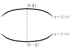
Figure 1. $\partial\Omega$ as a pair of local graphs

Our inverse results pertain to the following two classes of drumheads: (i) the class $\mathcal{D}_{1,L}$ of drumheads with one symmetry $\sigma$ and a bouncing ball orbit of length $2L$ which is reversed by $\sigma$; and (ii) the class $\mathcal{D}_{m,L}$ $(m\geq 2)$ of drumheads with the dihedral symmetry group $D_{m}$ and an invariant $m$-link reflecting ray. Let us define the classes more precisely and state the results.

1.1.1. Domains with one symmetry

The class $\mathcal{D}_{1,L}$ consists of simply connected real-analytic plane domains $\Omega$ satisfying:

• (i) There exists an isometric involution $\sigma$ of $\Omega$ which ‘reverses’ a non-degenerate bouncing ball orbit $\gamma\to\gamma^{-1}$ of length $L_{\gamma}=2L$. Hence $f_{+}(x)=-f_{-}(x)$;

• (ii) The lengths $2rL$ of all iterates $\gamma^{r}$ ($r=1,2,3,\dots$) have multiplicity one in $Lsp(\Omega)$, and in the elliptic case, the eigenvalues $e^{i\alpha}$ of the linear Poincare map $P_{\gamma}$ satisfy that $a=-2\cos\frac{\alpha}{2}$ does not belong to the ‘bad set’ ${\mathcal{B}}=\{a=0,-1,2,-2\}$.

• (iv) The endpoints of $\gamma$ are not vertices of $\partial\Omega$.

Figure 2. A domain in ${\mathcal{D}}_{1,L}$

Let Spec${}_{B}(\Omega)$ denote the spectrum of the Laplacian $\Delta_{\Omega}$ of the domain $\Omega$ with boundary conditions $B$ (Dirichlet or Neumann).

Theorem 1.1.

For Dirichlet (or Neumann) boundary conditions $B$, the map Spec${}_{B}:{\mathcal{D}}_{1,L}\mapsto{\mathbb{R}}_{+}^{{\bf N}}$ is 1-1.

Let us clarify the assumptions and consider related problems on ${\mathbb{Z}}_{2}$-symmetric domains:

(a) Under the up-down symmetry assumption, $f_{+}(x)=-f_{-}(x)$ (see Figure (2)). Hence there is ’only one’ analytic function $f$ to determine. It is quite a different problem if $\sigma$ preserves orientation of $\gamma$ (i.e. flips the domain left-right rather than up-down), which amounts to saying that $f_{\pm}$ are even functions but does not give a simple relation between them.

(b) Condition (ii) on the multiplicity of $2L$ means that $\gamma$ is the only closed billiard orbit of length $2L$. Since $\gamma=\gamma^{-1}$ for a bouncing ball orbit, the multiplicity is one rather than two. The method we use to calculate the trace combines the interior and exterior problems, and so one might think it necessary to assume that no exterior closed billiard trajectory (in the complement $\Omega^{c}$ of $\Omega$) has length $2L$. However, it is known that there exists a purely interior wave trace (cf. §1.2) and that the wave trace invariants at $\gamma$ are spectral invariants; we use the interior/exterior combination only to simplify the calculation. Therefore, it is not necessary to exclude exterior closed orbits of length $L$. When making stationary phase calculations, we only consider the interior closed orbits.

(c) The linear Poincaré map $P_{\gamma}$ is defined in §2. In the elliptic case, its eigenvalues $\{e^{\pm i\alpha}\}$ are of modulus one and we require that $a=-2\cos\frac{\alpha}{2}$ lies outside the bad set ${\mathcal{B}}$. In the hyperbolic case, its eigenvalues $\{e^{\pm\alpha}\}$ are real and they are never roots of unity in the non-degenerate case. These are generic conditions in the class of analytic domains. We refer to the angles $\alpha$ as Floquet angles. The set ${\mathcal{B}}$ consists of angle parameters where certain functions fail to be independent as one ‘iterates’ the geodesic $\gamma$. The role of this set will be described more precisely in §1.2.3.

(d) Assumption (iii) is equivalent to $f_{\pm}^{(3)}(0)\not=0$. The third derivatives $f_{\pm}^{(3)}(0)$ of $f_{\pm}$ at the endpoints of the bouncing ball orbit appear as coefficients of certain terms in the wave invariants, and we make assumption (iv) to ensure that the corresponding term does not vanish. Geometrically, $f_{\pm}^{(3)}(0)=0$ only if the endpoints of the bouncing ball orbit are vertices of $\partial\Omega$, i.e. critical points of the curvature. This is a technical condition which we believe can be removed by an extension of the argument, as will be discussed at the end of the proof. We do not give a complete argument for the sake of brevity.

As a corollary, we of course have the main result of [Z1, Z2, ISZ] that a simply connected analytic domain with the symmetries of an ellipse and with one axis of a prescribed length $L$ is spectrally determined within this class.

Corollary 1.2.

Let ${\mathcal{D}}_{2}$ be the class of analytic convex domains with central symmetry, i.e. the symmetries of an ellipse. Assume that $\{rL_{\gamma}\}$ are of multiplicity one in $Lsp(\Omega)$ up to time reversal ($r=1,2,3,\dots$). Then Spec_B: ${\mathcal{D}}\mapsto{\mathbb{R}}_{+}^{{\bf N}}$ is 1-1.

We give a new proof at the start of §6 since it is much simpler than the one-symmetry case and since the proof is simpler than the ones in [Z1, Z2].

This inverse result is also true for non-convex simply connected analytic domains with the symmetries of the ellipse if we assume one axis has length $L$ and is of multiplicity one. We stated the result only for convex domains because, by a recent result of M. Ghomi [Gh], the shortest closed trajectory of a centrally-symmetric convex domain is automatically a bouncing ball orbit, hence it is not necessary to mark the length $L$ of an invariant bouncing ball orbit.

Theorem (1.1) removes the (left/right) symmetry from the conditions on the domains considered in [Z1, Z2]. The situation for analytic plane domains is now quite analogous to that for analytic surfaces of revolution [Z3], where the rotational symmetry implies that the profile curve is up/down symmetric but not necessarily left/right symmetric.

Theorem 1.1 admits a generalization to the special piecewise analytic mirror symmetric domains with corners which are formed by reflecting the graph of an analytic function $y=f(x)$ around the $x$-axis. More precisely, let $f(x)$ be an analytic function on an interval $[-a,a]$ (for some $a$) such that $f(a)=f(-a)=0$ and that $f$ has no other zeros in $[-a,a]$. Then consider the domain $\Omega_{f}$ bounded by the union of the graphs $y=\pm f(x)$.

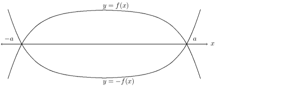
Figure 3. ${\mathbb{Z}}_{2}$ symmetric domain with corners

Let ${\mathcal{F}}$ be the class of real analytic functions with the stated properties, and consider those $f$ for which precisely one critical value of $f$ equals $L/2$. The vertical line through $(x,\pm L/2)$ is then a bouncing ball orbit. We further impose the same generic conditions on $\Omega_{f}$ as in Theorem 1.1. We denote the resulting class of real analytic graphs by ${\mathcal{F}}_{L}$.

Theorem 1.3.

Up to translation (i.e. choice of $a$), the Dirichlet (or Neumann) spectrum of $\Omega_{f}$ determines $f$ within ${\mathcal{F}}_{L}$, i.e.: Spec$:{\mathcal{F}}_{L}\mapsto{\mathbb{R}}_{+}^{{\bf N}}$ is 1-1.

The proof is identical to that of Theorem 1.1 once it is established that there exists a wave trace expansion around the length $t=2L$ of the bouncing ball orbit for domains in ${\mathcal{F}}$ with the same coefficients as in the smooth case. This fact follows from work of A. Vasy [V] on the Poisson relation for manifolds with corners. In other words, the presence of corners does not affect the wave trace expansion at the bouncing ball orbit.

1.1.2. Dihedrally symmetric domains

The second class of domains is the class $\mathcal{D}_{m,L}$ of dihedrally symmetric analytic drumheads $\Omega$, i.e. domains satisfying:

• (i) $\tau\Omega=\Omega$ for all $\tau\in D_{m}$;

• (ii) $D_{m}$ leaves invariant at least one $m$-link periodic reflecting ray $\gamma$ of length $2L$;

• (iii) The lengths $2rL$ have multiplicity one in $Lsp(\Omega)$

Figure 4. A $D_{3}$-symmetric domain

We then have:

Theorem 1.4.

For any $m\geq 2$, Spec${}_{B}:{\mathcal{D}}_{m,L}\mapsto{\mathbb{R}}_{+}^{{\bf N}}$ is 1-1.

We recall that $D_{m}$ is the group generated by elements $\{\sigma,R_{2\pi/m}\}$ where $R_{2\pi/m}$ is counter-clockwise rotation through the angle $2\pi/m$ and where $\sigma^{2}=1$, with the relations $\sigma R_{2\pi/n}\sigma=R_{-2\pi/n}.$ Also, by an $m$-link periodic reflecting ray we mean a periodic billiard trajectory with $m$ points of transversal reflection off $\partial\Omega.$ It is easy to see that such a ray exists if $\Omega$ is convex. In general, it is a non-trivial additional assumption. With this proviso, Theorem (1.4) is a second kind of generalization of the inverse spectral result of [Z1, Z2] for the class ${\mathcal{D}}_{2,L}$ of ‘bi-axisymmetric domains’. That result obviously covers the classes ${\mathcal{D}}_{2n,L}$, but the general case is new. For any prime $p$, the result for ${\mathcal{D}}_{p,L}$ is independent of any other case where $p$ does not divide $n$.

1.2. Overview

Let us give a brief overview of the proofs.

We denote by

$$E_{B}^{\Omega}(t,x,y)=\sum_{j}\cos t\lambda_{j}\varphi_{j}(x)\varphi_{j}(y)$$

the kernel of the even part of the wave group $\cos t\sqrt{\Delta_{B}^{\Omega}}$, generated by the Laplacian $\Delta_{B}^{\Omega}$ of (1) with either Dirichlet $Bu=u|_{\partial\Omega}$ or Neumann $Bu=\partial_{\nu}u|_{\partial\Omega}$ boundary conditions. Its distribution trace is defined by

(3) $$Tr1_{\Omega}E_{B}^{\Omega}(t):=\int_{\Omega}E_{B}^{\Omega}(t,x,x)dx=\sum_{j=1}^{\infty}\cos t\lambda_{j}$$

When $L_{\gamma}$ is the length of a non-degenerate periodic reflecting ray $\gamma$ of the generalized billiard flow, and when the only periodic orbits of length $L_{\gamma}$ are $\gamma$ and $\gamma^{-1}$ (the time-reversal of $\gamma$), then $Tr1_{\Omega}E_{B}^{\Omega}(t)$ is a Lagrangian distribution in the interval $(L_{\gamma}-\epsilon,L_{\gamma}+\epsilon)$ for sufficiently small $\epsilon$, and has the following expansion in terms of homogeneous singularities: (see [GM], Theorem 1, and also page 228; see also [PS] Theorem 6.3.1).

Let $\gamma$ be a non-degenerate billiard trajectory whose length $L_{\gamma}$ is isolated and of multiplicity one in $Lsp(\Omega)$. Then for $t$ near $L_{\gamma}$, the trace of the even part of the wave group has the singularity expansion

(4) $$Tr1_{\Omega}E_{B}^{\Omega}(t)\sim\Re\{a_{\gamma}(t-L_{\gamma}+i0)^{-1}+a_{\gamma 0}\log(t-L_{\gamma}+i0)+\sum_{k=1}^{\infty}a_{\gamma k}(t-L_{\gamma}+i0)^{k}\log(t-L_{\gamma}+i0)\},$$

where the coefficients $a_{\gamma k}$ (the wave trace invariants) are calculated by the stationary phase method from a microlocal parametrix for $E_{B}^{\Omega}$ at $\gamma$.

Here, $a_{\gamma}$ is a sum of the contributions from $\gamma$ and $\gamma^{-1}$, which are the same. In general, the contribution at $t=L_{\gamma}$ is the sum over all periodic orbits of length $L_{\gamma}$. The sum to the right of $\Re$ is the trace of the wave group $e^{it\sqrt{\Delta_{B}^{\Omega}}}$; the trace of the even part $E_{B}^{\Omega}(t)$ of the wave group equals the real part of that trace.

In [Z5], §3.1, this expansion was reformulated in terms of a regularized trace of the interior resolvent $R_{B}^{\Omega}(k+i\tau)=-(\Delta^{\Omega}_{B}+(k+i\tau)^{2})^{-1}:H^{s}(\Omega)\to H^{s+2}(\Omega)$, with $k\in{\mathbb{R}},\tau>0$ and with boundary condition $B$. The Schwartz kernel or Green’s kernel $G_{B}^{\Omega}(k+i\tau,x,y)\in\mathcal{D}^{\prime}(\Omega\times\Omega)$ of the resolvent is the unique solution of the boundary problem:

(5) $$\left\{\begin{array}[]{l}-(\Delta^{\Omega}_{B}+(k+i\tau)^{2})G_{B}^{\Omega}(k+i\tau,x,y)=\delta_{y}(x),\;\;\;(x,y\in\Omega)\\ \\ BG_{B}^{\Omega}(k+i\tau,x,y)=0,\;\;\;x\in\partial\Omega\end{array}\right.$$

Let $\hat{\rho}\in C_{0}^{\infty}(L_{\gamma}-\epsilon,L_{\gamma}+\epsilon)$ be a cutoff, equal to one on an interval $(L_{\gamma}-\epsilon/2,L_{\gamma}+\epsilon/2)$ which contains no other lengths in Lsp$(\Omega)$ occur in its support, and define the smoothed (and localized) resolvent with a choice of boundary conditions by

(6) $$R_{B\rho}^{\Omega}(k+i\tau):=\int_{{\mathbb{R}}}\rho(k-\mu)(\mu+i\tau)R_{B}^{\Omega}(\mu+i\tau)d\mu.$$

The definition is chosen so that

(7) $$R_{B\rho}^{\Omega}(k+i\tau)=\int_{0}^{\infty}\hat{\rho}(t)e^{i(k+i\tau)t}E_{B}^{\Omega}(t)dt.$$

Then the smoothed resolvent trace admits an asymptotic expansion of the form

(8) $$Tr1_{\Omega}R_{B\rho}^{\Omega}(k+i\tau)\sim{\mathcal{D}}_{B,\gamma}(k+i\tau)\sum_{j=0}^{\infty}B_{\gamma,j}k^{-j},\;\;\;k\to\infty,$$

where

• ${\mathcal{D}}_{B,\gamma}(k+i\tau)$ is the symplectic pre-factor

  $${\mathcal{D}}_{B,\gamma}(k+i\tau)=C_{0}\;\epsilon_{B}(\gamma)\frac{e^{i(k+i\tau)L_{\gamma}}e^{i\frac{\pi}{4}m_{\gamma}}}{\sqrt{|\det(I-P_{\gamma})|}}$$

• $P_{\gamma}$ is the Poincaré map associated to $\gamma$ (see §2 for background);

• $\epsilon_{B}(\gamma)$ is the signed number of intersections of $\gamma$ with $\partial\Omega$ (the sign depends on the boundary conditions; $\pm 1$ for each bounce for Neumann/Dirichlet boundary conditions);

• $m_{\gamma}$ is the Maslov index of $\gamma$;

• $C_{0}$ is a universal constant (e.g. factors of $2\pi$) which it is not necessary to know for the proof of Theorem 1.1.

The resolvent trace (or Balian-Bloch) coefficient $B_{\gamma,j}$ associated to a periodic orbits $\gamma,\gamma^{-1}$ is easily related to the wave trace coefficient $a_{\gamma,k}$. We henceforth work solely with the expansion (8), which we term the ‘Balian-Bloch expansion’ after [BB2]. In fact, we actually analyze the closely related resolvent trace asymptotics along logarithmic curves $k+i\tau\log k$ in the upper half plane. It is clear that the ‘Balian-Bloch coefficients’ $B_{\gamma,j}$ are spectral invariants and it is these invariants we use in our inverse spectral results.

As mentioned above, the inverse results have three main ingredients, which we now describe in detail as a guide to the paper and its connections to [Z4, Z5].

1.2.1. Reduction to boundary oscillatory integrals of the wave trace

The first step (Theorem 3.1) is a reduction to the boundary of the wave trace. This reduction was largely achieved in [Z5, Z4] by means of a rigorous version of the Balian-Bloch approach to the Poisson relation between spectrum and closed billiard orbits [BB1, BB2]. It expresses the wave trace localized at the length of a periodic reflecting ray, up to a given order of singularity, as a finite sum of oscillatory integrals $I_{M,\rho}^{\sigma,w}(k+i\tau)$ over the boundary (see (19). It is related in spirit to the monodromy operator approach of [SZ, ISZ].

1.2.2. Feynman diagram analysis and proof of Theorem 4.2

The second ingredient is a stationary phase analysis of the oscillatory integral expressions for the wave invariants at transversally reflecting periodic orbits. The key role is played by a (Feynman) diagrammatic analysis of the stationary phase expansions, which has not previously been used in inverse spectral theory (see [AG] for prior use in calculated the sub-principal invariant). As reviewed in §5.1, the terms of stationary phase expansion correspond to labelled graphs $\Gamma$ and the coefficients of the stationary phase expansion can be expressed as ‘Feynman amplitudes’ determined by the graphs $\Gamma$. The Euler characteristic of $\Gamma$ corresponds to the power $k^{-j}$ of $k$ in the wave trace expansion.

The inverse spectral problem involves a novel point of the diagrammatic analysis: namely, to separate out the (labelled graphs) of Euler characteristic $-j$ whose amplitudes contain the maximum numbers ($2j+2,2j-1$) of derivatives of $\partial\Omega.$ In Theorem 4.2 we prove that the terms in a given wave invariant which contain the maximal number of derivatives of $\partial\Omega$ only arise in the stationary phase expansion of one principal term and its time reversal, whose amplitudes have special properties stated in table in Theorem 4.2. The principal terms are defined in Definition 4.3. Only the special properties of the phase and amplitude are used in the calculation of the wave trace invariants.

The analysis leads to the explicit formulae for the top derivative parts of the wave invariants at iterates of bouncing ball orbits in Theorem 5.1. For instance, in the symmetric bouncing ball case there is only one important diagram for the even derivatives $f^{(2j)}(0)$ and two important diagrams for the odd derivatives $f^{(2j-1)}(0)$. Modulo terms involving $\leq 2j-2$ derivatives, the wave trace (or more precisely resolvent trace) invariants (cf. (4)-(8) $B_{\gamma^{r},j-1}$ take the form (cf. Corollary 5.11):

(9) $$\begin{array}[]{lll}B_{\gamma^{r},j-1}&=&(4Lr){\mathcal{A}}_{r}(0)i^{j-1}\{2(w_{{\mathcal{G}}_{1,j}^{2j,0}})\;(h_{2r}^{11})^{j}f^{(2j)}(0)\\ &&\\ &&+4(w_{{\mathcal{G}}_{2,j+1}^{2j-1,3,0}})\;(h_{2r}^{11})^{j}\frac{1}{2-2\cos\alpha/2}(f^{(3)}(0)f^{(2j-1)}(0))\\ &&\\ &&+4(w_{\widehat{{\mathcal{G}}}_{2,j+1}^{2j-1,3,0}})\;(h_{2r}^{11})^{j-2}\sum_{q=1}^{2r}(h_{2r}^{1q})^{3}(f^{(3)}(0)f^{(2j-1)}(0))\}.\end{array}$$

Here and throughout the paper we use the following notational conventions:

• $h_{2r}^{pq}$ are the matrix elements of the inverse of the Hessian $H_{2r}$ of the length function ${\mathcal{L}}$ in Cartesian graph coordinates at $\gamma^{r}$ (cf. §2).

• ${\mathcal{A}}_{r}(0)$ is an $\Omega$-independent (non-zero) constant obtained from amplitude of the principal terms at the critical bouncing ball orbit.

• $w_{{\mathcal{G}}_{1,j}^{2j,0}}$ (etc.) are certain non-zero combinatorial constants associated to Feynman graphs denoted here by ${\mathcal{G}}_{1,j}^{2j,0}$ etc. For a given graph ${\mathcal{G}}$, $w_{{\mathcal{G}}}=\frac{1}{|Aut({\mathcal{G}})|}$ where $|Aut({\mathcal{G}})|$ is the order of the symmetry group of the graph; see the discussion after (56).

The amplitude value ${\mathcal{A}}_{r}(0)$ and the Wick constants may be evaluated explicitly. However it is not necessary for the proof of Theorem 1.1 to do so and it seems more illuminating to specify the origins, rather than their values, of the various constants. We note that the $h_{2r}^{ij}$ depend on, and only on, $r$ and the eigenvalues of the Poincaré map $P_{\gamma}$ (i.e. on the Floquet angles) and on the length of $\gamma$. We also note that $\gamma=\gamma^{-1}$ when $\gamma$ is a bouncing-ball orbit (such an orbit is called reciprocal).

The analysis shows that the non-principal oscillatory integrals only give rise to sub-maximal derivative terms in the wave invariants, completing the proof of Theorem 4.2.

1.2.3. Inverse results

The third ingredient is the analysis of the top derivative terms in the wave trace invariants in the symmetry classes above. The key point is determine the $2j-1$st and $2j$th Taylor coefficients of the curvature at each reflection point from the $j-1$st wave trace invariant for $\gamma$ and its iterates $\gamma^{r}.$

We note that the previously known inverse result for analytic domains with the symmetry of an ellipse drops out immediately from (9), since the odd Taylor coefficients are zero. On the other hand, there is an obstruction to recovering the Taylor coefficients of $f$ when there is only one symmetry: namely, we must recover two Taylor coefficients $f^{(2j)}(0),f^{(2j-1)}(0)$ for each new value of $j$ (the degree of the singularity). This is the principal obstacle to overcome.

We overcome it in §6 as follows: The expression (9) for the Balian-Bloch invariants of $\gamma,\gamma^{2},\dots$ consists of two types of terms, in terms of their dependence on the iterate $r$. They have a common factor of $2rL(h_{2r}^{11})^{j-2}{\mathcal{A}}_{r}(0)$, and after factoring it out we obtain one term

$$(h_{2r}^{11})^{2}\{(w_{{\mathcal{G}}_{1,j}^{2j,0}})f^{(2j)}(0)+\frac{(w_{{\mathcal{G}}_{2,j+1}^{2j-1,3,0}})}{2-2\cos\alpha/2}f^{(3)}(0)f^{(2j-1)}(0)\}$$

which depends on the iterate $r$ through the coefficient $(h_{2r}^{11})^{2}$, and one

$$(w_{\widehat{{\mathcal{G}}}_{2,j+1}^{2j-1,3,0}})\left(\sum_{q=1}^{2r}(h_{2r}^{1q})^{3}f^{(3)}(0)f^{(2j-1)}(0)\right)$$

which depends on $r$ through the cubic sums $\sum_{q=1}^{2r}(h_{2r}^{1q})^{3}$ of inverse Hessian matrix elements $h_{2r}^{pq}$. In order to ‘decouple’ the even and odd derivatives, it suffices to show that the functions $(h_{2r}^{11})^{2}$ and $\sum_{q=1}^{2r}(h_{2r}^{1q})^{3}$ are, at least for ‘most’ Floquet angles $\alpha$, linearly independent as functions of $r\in{\mathbb{Z}}$, i.e. that $(h_{2r}^{11})^{-2}\sum_{q=1}^{2r}(h_{2r}^{1q})^{3}$ is a non-constant function of $r$. It is convenient to use the parameter $a=-2\cos\frac{\alpha}{2}$ and we write the dependence as $h_{2r}^{ij}(a)$.

We therefore define the ‘bad’ set of Floquet angles by

(10) $${\mathcal{B}}=\{a:\;\;\mbox{the sequence }\;\{(h_{2r}^{11}(a))^{-2}\sum_{q=1}^{2r}(h_{2r}^{1q}(a))^{3},\;\;r=1,2,3,\dots\}\;\mbox{is constant in }\;r\}.$$

Using facts about the finite Fourier transform and circulant matrices, we compute that ${\mathcal{B}}=\{0,1,\pm 2\}.$ Since the proof is computational, we also present a simple conceputal argument (cf. Proposition 6.7)that ${\mathcal{B}}$ is finite, although the proof only gives the poor estimate $3^{20}$ on its number of elements. For Floquet angles outside of ${\mathcal{B}}$, we can determine all Taylor coefficients $f_{+}^{(j)}(0)$ from the wave invariants and hence the analytic domain.

We use a similar strategy in the dihedral $D_{n}$-case in §7. Due to the extra symmetries, the inverse results in the dihedral case require much less information about the wave invariants than in the one symmetry case.

1.3. Related results

(i) We have already mentioned the prior result that analytic drumheads with up/down and left/right symmetries are spectrally determined in that class [Z1, Z2]. Previously, it was proved by Colin de Verdiere [CV] that such domains are spectrally rigid. To our knowledge, the only other prior result giving a ‘large’ class of spectrally domains is that of Marvizi-Melrose [MM1], in which members of a spectrally determined two-parameter family of convex plane domains are determined among generic convex domains by their spectra.

(ii) In [Z4], we extend the inverse result to the exterior problem of determining a ${\mathbb{Z}}_{2}$-symmetric configuration of analytic obstacles from its scattering phase (or resonance poles). Our result may be stated as follows: Let $\Omega={\mathbb{R}}^{2}-\{{\mathcal{O}}\cup\tau_{x,L}{\mathcal{O}}\}$ where ${\mathcal{O}}$ is a convex analytic obstacle, where $x\in{\mathcal{O}}$ and where $\tau_{x,L}$ is the mirror reflection across the orthogonal line segment of length $L$ from $x$. Thus, $\{{\mathcal{O}}\cup\tau_{x,L}({\mathcal{O}})\}$ is a ${\mathbb{Z}}_{2}$-symmetric obstacle consisting of two components. Let $\Delta_{\Omega}$ denote the Dirichlet Laplacian on $\Omega.$ We have:

Theorem 1.5.

[Z4] With the same genericity assumptions as in Theorem 1.1, the resonance poles of $\Delta_{\Omega}$ determine ${\mathcal{O}}$ within the class of ${\mathbb{Z}}_{2}$ symmetric analytic obstacles.

1.4. Future directions

An obvious future direction is to study the wave invariants without any symmetry assumptions. As will become clear from the calculations in this article (cf. Theorems 4.2 and 3.1), symmetries make ‘lower order derivative data’ in wave invariants redundant and allow one to concentrate on terms in a given wave invariant with maximal numbers of derivatives. Lacking symmetries, the lower order derivative data is no longer redundant and one has to navigate a complicated jungle of terms to determine which combinations are spectral invariants. It is plausible that one cannot work with just one orbit but must combine information from two bouncing ball orbits (they always exist in a convex plane domain). The main problem is then to extract from the wave invariants of the iterates of each bouncing ball orbit sufficient Taylor series data at the endpoints to determine the domain. To do this, it seems necessary to analyze how Feynman amplitudes of labelled diagrams behave as a function of the iterate $r$ of the orbits. The graphs themselves do not depend on $r$, so the dependence comes from the labelling.

1.5. Acknowledgements

The first draft of this article was posted in 2001 (arXiv math.SP/0111078) as part of the series now published as [Z4, Z5]. In the intervening period, some of the computational details of this article have received independent confirmation. R. Bacher found an independent proof corroborating the result of §5 that only five graphs in the Feynman diagrammatics have the right form to contribute to the highest order data [B]. C. Hillar did a numerical study of the circulant sums of §6 to corroborate that the nonlinear power sums have nonlinear $r$ dependence as $r\to\infty$. A. Vasy and J. Wunsch gave advice on [V]. We thank Y. Colin de Verdière and the spectral theory seminar at Grenoble for their patience in listening to earlier versions of this article and for their comments. Especially, we thank the referee for many remarks and corrections. The referee pointed out that ‘bad set’ ${\mathcal{B}}$ could be explicitly calculated, and the calculations were done by H. Hezari. We thank H. Hezari as well for carefully reading the final version.

Contents

1. 1 Introduction
   1. 1.1 Statement of results
      1. 1.1.1 Domains with one symmetry
      2. 1.1.2 Dihedrally symmetric domains
   2. 1.2 Overview
      1. 1.2.1 Reduction to boundary oscillatory integrals of the wave trace
      2. 1.2.2 Feynman diagram analysis and proof of Theorem 4.2
      3. 1.2.3 Inverse results
   3. 1.3 Related results
   4. 1.4 Future directions
   5. 1.5 Acknowledgements
2. 2 Billiards and the length functional
   1. 2.1 Cartesian coordinates around bouncing ball orbits
3. 3 Resolvent trace invariants
   1. 3.1 Proof of Theorem 3.1
      1. 3.1.1 Completion of proof of Theorem 3.1
4. 4 Principal term of the Balian-Bloch trace
   1. 4.1 Key properties of the principal amplitude and phase
      1. 4.1.1 Further properties of the amplitude and phase
   2. 4.2 Comparison with [Z5]
5. 5 Feynman diagrams in inverse spectral theory
   1. 5.1 Stationary phase diagrammatics
      1. 5.1.1 Stationary phase formula for $I_{M,\rho}^{\sigma,w_{\pm}}$
   2. 5.2 Maximal derivative terms
   3. 5.3 The principal terms
      1. 5.3.1 The principal term: The data $f_{\pm}^{2j}(0)$
      2. 5.3.2 The principal term: The data $f_{\pm}^{(2j-1)}(0)$
   4. 5.4 Non-principal terms
   5. 5.5 Appendix: Non-contributing diagrams
   6. 5.6 Balian-Bloch invariants at bouncing ball orbits of up-down symmetric domains
6. 6 Proof of Theorem (1.1)
   1. 6.1 Completion of the proof of Theorem 1.1
   2. 6.2 Circulant Hessian at ${\mathbb{Z}}_{2}$-symmetric bouncing ball orbits
   3. 6.3 Diagonalizing $H_{2r}^{-1}$
   4. 6.4 Matrix elements of $H_{2r}^{-1}$ at a ${\mathbb{Z}}_{2}$-symmetric bouncing ball orbit
   5. 6.5 Linear sums
   6. 6.6 Decoupling Balian-Bloch invariants
   7. 6.7 Cubic Hessian sums
      1. 6.7.1 First proof of Proposition 6.7: Dedekind sums
      2. 6.7.2 Second proof: Explicit inversion of the Hessian
   8. 6.8 Final step in proof of Theorem 1.1: Inductive determination of Taylor coefficients
   9. 6.9 The case where $f^{(3)}(0)=0$
7. 7 Proof of Theorem (1.4)
   1. 7.1 Structure of coefficients at a $D_{m}$-ray
      1. 7.1.1 $D_{m}$-rays
   2. 7.2 The principal terms
      1. 7.2.1 The principal term: The data $f^{2j}(0)$
   3. 7.3 Dihedral domains: Proof of Theorem (1.4)

2. Billiards and the length functional

We begin by establishing notation on plane billiards and length functions. After recalling basic notions, we calculate the Hessian of the length functional at iterates of a critical bouncing ball orbit in Cartesian coordinates adpated to the orbit.

We denote by $\Omega$ a simply connected analytic plane domain with boundary $\partial\Omega$ of length $2\pi$. The billiard flow $\Phi^{t}$ of $\Omega$ is the broken geodesic of the Euclidean metric on $\Omega$. That is, for $(x,\xi)\in T^{*}\Omega^{o}$, the trajectory $\Phi^{t}(x,\xi)$ follows the Euclidean straight line in the interior $\Omega^{o}$ of $\Omega$ and reflects from the boundary by Snell’s law of equal angles. By the billiard map $\beta$ of $\Omega$ we mean the map on $B^{*}\partial\Omega$ induced by $\Phi^{t}$: we add a multiple of the inward unit normal $\nu_{q}$ to $(q,\eta)\in B^{*}(\partial\Omega)$ to obtain an inward pointing unit vector $v$ at $q$. We then follow the billiard trajectory $\Phi^{t}(q,v)$ until it hits the boundary, and then define $\beta(q,\eta)$ to be its tangential projection. We refer to [PS, KT, Z5] for details and discussions of the billiard flow on domains in ${\mathbb{R}}^{2}$.

It is natural at first to parametrize $\partial\Omega$ by arclength,

(11) $$q:{\bf T}\to\partial\Omega\subset{\mathbb{R}}^{2},$$

starting at some point $q_{0}\in\partial\Omega$. Here, ${\bf T}={\mathbb{R}}\backslash 2\pi{\mathbb{Z}}$ denotes the unit circle. By an $m$-link periodic reflecting ray of $\Omega$ we mean a periodic billiard trajectory $\gamma$ which intersects $\partial\Omega$ transversally at $m$ points $q(\varphi_{1}),\dots,q(\varphi_{m})$, and reflects off $\partial\Omega$ at each point according to Snell’s law

(12) $$\frac{q(\varphi_{j+1})-q(\varphi_{j})}{|q(\varphi_{j+1})-q(\varphi_{j})|}\cdot\nu_{q(\varphi_{j})}=\frac{q(\varphi_{j})-q(\varphi_{j-1})}{|q(\varphi_{j})-q(\varphi_{j-1})|}\cdot\nu_{q(\varphi_{j})}.$$

Here, $\nu_{q(\varphi)}$ is the inward unit normal to $\partial\Omega$ at $q(\varphi)$. We refer to the segments $q(\varphi_{j})-q(\varphi_{j-1})$ as the links of the trajectory. We denote the acute angle between the link $q(\varphi_{j+1})-q(\varphi_{j})$ and the inward unit normal $\nu_{q(\varphi_{j})}$ by $\angle(q(\varphi_{j+1})-q(\varphi_{j}),\nu_{q(\varphi_{j})})$ and that between $q(\varphi_{j})-q(\varphi_{j-1})$ and the inward unit normal at $q(\varphi_{j})$ by $\angle(q(\varphi_{j})-q(\varphi_{j-1}),\nu_{q(\varphi_{j})})$, i.e. we put

(13) $$\frac{q(\varphi_{j+1})-q(\varphi_{j})}{|q(\varphi_{j+1})-q(\varphi_{j})|}\cdot\nu_{q(\varphi_{j})}=\cos\angle(q(\varphi_{j+1})-q(\varphi_{j}),\nu_{q(\varphi_{j})}).$$

For notational simplicity we often do not distinguish between a billiard trajectory in $S^{*}\Omega$ and its projection to $\Omega$.

We define the length functional on ${\bf T}^{M}$ by:

(14) $$L(\varphi_{1},\dots,\varphi_{M})=|q(\varphi_{1})-q(\varphi_{2})|+\dots+|q(\varphi_{M-1})-q(\varphi_{M})|+|q(\varphi_{M})-q(\varphi_{1})|.$$

We often use cyclic index notation where $q(\varphi_{M+1})=q(\varphi_{1}).$ It is clear that $L$ is a smooth function away from the ‘large diagonals’ $\Delta_{j,j+1}:=\{\varphi_{j}=\varphi_{j+1}\}$, where it has $|x|$ singularities. We have:

(15) $$\begin{array}[]{l}\frac{\partial}{\partial\varphi_{j}}|q(\varphi_{j})-q(\varphi_{j-1})|=-\sin\angle(q(\varphi_{j})-q(\varphi_{j-1}),\nu_{q(\varphi_{j})}),\\ \\ \frac{\partial}{\partial\varphi_{j}}|q(\varphi_{j})-q(\varphi_{j+1})|=\sin\angle(q(\varphi_{j+1})-q(\varphi_{j}),\nu_{q(\varphi_{j})})\\ \\ \implies\frac{\partial}{\partial\varphi_{j}}L=\sin\angle(q(\varphi_{j+1})-q(\varphi_{j}),\nu_{q(\varphi_{j})})-\sin\angle(q(\varphi_{j})-q(\varphi_{j-1}),\nu_{q(\varphi_{j})}).\end{array}$$

Hence, the condition that $\frac{\partial}{\partial\varphi_{j}}L=0$ is the same as (12) for the $2$-link defined by the triplet $(q(\varphi_{j-1}),q(\varphi_{j}),q(\varphi_{j+1}))$.

Let $\gamma$ denote a periodic reflecting ray of $\Omega$. The linear Poincare map $P_{\gamma}$ of $\gamma$ is the derivative at $\gamma(0)$ of the first return map to a transversal to $\Phi^{t}$ at $\gamma(0).$ By a non-degenerate periodic reflecting ray $\gamma$ we mean one whose linear Poincaré map $P_{\gamma}$ has no eigenvalue equal to one (cf. [PS, KT]). The following relates $P_{\gamma}$ and the Hessian of the length functional in angular coordinates:

Proposition 2.1.

([KT] (Theorem 3)) Let $H_{n}^{a}$ denote the Hessian of $L$ in angular coordinates $\varphi_{j}$ at a critical point $\gamma$, and let $b_{j}=\frac{\partial^{2}|q(\varphi_{j+1})-q(\varphi_{j})|}{\partial\varphi_{j}\partial\varphi_{j+1}}.$ Then

$$\det(I-P_{\gamma})=-\det(-H_{n}^{a})\cdot(b_{1}\cdots b_{n})^{-1}.$$

This identity may be proved by expressing both sides in terms of bases of horizontal and vertical Jacobi fields.

2.1. Cartesian coordinates around bouncing ball orbits

We now specialize to the case where $\gamma$ is a bouncing ball orbits (i.e. $2$-link periodic reflecting rays). As in the Introduction, we orient $\Omega$ so that the bouncing ball orbit is along the $y$-axis with endpoints $A=(0,\frac{L}{2}),B=(0,-\frac{L}{2})$ and parametrize $\partial\Omega$ near $A$ by $y=f_{+}(x)$ and near $B$ by $y=f_{-}(x)$. We do not assume the domain is up-down symmetric.

We denote by $R_{A}$, resp. $R_{B}$, the radius of curvature of $\Omega$ at the endpoints $A,B$. When $\gamma$ is elliptic, the eigenvalues of $P_{\gamma}$ are of the form $\{e^{\pm i\alpha}\}$ ($\alpha\in{\mathbb{R}}$) while in the hyperbolic case they are of the form $\{e^{\pm\alpha}\}$ ($\alpha\in{\mathbb{R}})$. They are given by the same formulae in both elliptic and hyperbolic cases:

(16) $$\left\{\begin{array}[]{ll}\cos(\alpha/2)=\sqrt{(1-\frac{L}{R_{A}})(1-\frac{L}{R_{B}})},&\;\;(\mbox{elliptic case}),\\ \\ \cosh(\alpha/2)=\sqrt{(1-\frac{L}{R_{A}})(1-\frac{L}{R_{B}})},&\;\;(\mbox{hyperbolic case}).\end{array}\right.$$

We define the length functionals in Cartesian coordinates for the two possible orientations of the $r$th iterate of a bouncing ball orbit by

(17) $${\mathcal{L}}_{\pm}(x_{1},\dots,x_{2r})=\sum_{j=1}^{2r}\sqrt{(x_{j+1}-x_{j})^{2}+(f_{w_{\pm}(j+1)}(x_{j+1})-f_{w_{\pm}(j)}(x_{j}))^{2}}.$$

Here, $w_{\pm}:{\mathbb{Z}}_{2r}\to\{\pm\}$, where $w_{+}(j)$ (resp. $w_{-}(j))$ alternates sign starting with $w_{+}(1)=+$ (resp. $w_{-}(1)=-$). Also, we use cylic index notation where $x_{2r+1}=x_{1}$.

We have:

(18) $$\begin{array}[]{lll}\frac{\partial{\mathcal{L}}_{\pm}}{\partial x_{j}}&=&\frac{(x_{j}-x_{j+1})+(f_{w_{\pm}(j)}(x_{j})-f_{w_{\pm}(j+1)}(x_{j+1}))f_{w_{\pm}(j)}^{\prime}(x_{j})}{\sqrt{(x_{j}-x_{j+1})^{2}+(f_{w_{\pm}(j)}(x_{j})-f_{w_{\pm}(j+1)}(x_{j+1}))^{2}}}\\ &&\\ &&-\frac{(x_{j-1}-x_{j})+(f_{w_{\pm}(j-1)}(x_{j-1})-f_{w_{\pm}(j)}(x_{j}))f_{w_{\pm}(j)}^{\prime}(x_{j})}{\sqrt{(x_{j}-x_{j-1})^{2}+(f_{w_{\pm}(j)}(x_{j})-f_{w_{\pm}(j-1)}(x_{j-1}))^{2}}}.\end{array}$$

We will need formulae for the entries of the Hessian of ${\mathcal{L}}_{+}$ at its critical point $(x_{1},\dots,x_{2r})=0$ in Cartesian coordinates corresponding to the $r$th repetition of a bouncing ball orbit.

Proposition 2.2.

Put

$$a=-2(1+Lf_{+}^{\prime\prime}(0))=-2(1-\frac{L}{R_{A}}),\;b=-2(1-Lf_{-}^{\prime\prime}(0))=-2(1-\frac{L}{R_{B}}).$$

Then the Hessian $H_{2r}$ of ${\mathcal{L}}_{+}$ at $x=0$ in Cartesian graph coordinates has the form $H_{2}=\frac{-1}{L}\begin{pmatrix}a&2\\ &\\ 2&b\end{pmatrix}$ for $r=1$ and for $r\geq 2$,

$$H_{2r}=\frac{-1}{L}\left\{\begin{array}[]{lllll}a&1&0&\dots&1\\ &&&&\\ 1&b&1&\dots&0\\ &&&&\\ 0&1&a&1&0\\ &&&&\\ 0&0&1&b&1\dots\\ &&&&\\ \dots&\dots&\dots&\dots&\dots\\ &&&&\\ 1&0&0&\dots&b\end{array}\right\}$$

.

Proof.

A routine calculation gives

$$\left\{\begin{array}[]{l}\frac{\partial^{2}{\mathcal{L}}_{+}}{\partial x_{j}^{2}}(0)=2(\frac{1}{L}+w_{+}(j)f_{w_{+}(j)}^{\prime\prime}(0)),\\ \\ \frac{\partial^{2}{\mathcal{L}}_{+}}{\partial x_{j}\partial x_{j+1}}(0)=\frac{-1}{L}\end{array}\right.$$

for $r\geq 2$. In the case of $r=1$, the length functional is $2||(x_{1},f_{+}(x_{1}))-(x_{2},f_{-}(x_{2}))||$. Note that for $r\geq 2$, there are two terms of ${\mathcal{L}}_{+}$ contributing to each diagonal matrix element and one to each off-diagonal element, accounting for the additional factor of $2$ in the diagonal terms. Also note that $f_{w_{+}(j)}(0)-f_{w_{+}(j+1)}(0)=w_{+}(j)L$ and that $f_{+}^{\prime\prime}(0)=\frac{-1}{R_{A}},f_{-}^{\prime\prime}(0)=\frac{1}{R_{B}}.$

∎

We remark that the Hessian in Cartesian coordinates in Proposition 2.2 differs from that in angular coordinates in [KT] in that the off-diagonal entries differ in sign. This is because the graph parametrization gives the opposite orientation to the tangent $T_{A}\partial\Omega$ than the angular parametrization and the same orientation at $T_{B}\partial\Omega$. The angular Hessian $H^{a}_{2r}$ is related to the Cartesian Hessian $H_{2r}$ by $H_{2r}^{a}=JH_{2r}J^{t}$ where $J=diag(1,-1,1,-1,\dots,1,-1)$ is the change of basis matrix. Clearly, the determinants of the two Hessians agree. Since $b_{j}=\frac{-1}{L}$, we obtain from Proposition 2.1 the following:

Corollary 2.3.

As above, let $H_{2r}$ denote the Hessian of ${\mathcal{L}}_{+}$ in Cartesian coordinates at the $r$th iterate $\gamma^{r}$ of a bouncing ball orbit $\gamma$ of length $2L$. Then

$$\det(I-P_{\gamma^{r}})=-L^{2r}\det(H_{2r}).$$

The determinant $\det H_{2r}$ is a polynomial in $\cos\frac{\alpha}{2}$ (elliptic case), resp. $\cosh\frac{\alpha}{2}$ (hyperbolic case) of degree $2r$. In the following we restrict to the elliptic case.

Proposition 2.4.

We have

$$\det H_{2r}=-L^{-2r}(2-2\cos r\alpha).$$

Proof.

Let $\lambda_{r},\lambda_{r}^{-1}$ be the eigenvalues of $P_{\gamma^{r}}$, so that $det(I-P_{\gamma^{r}})=2-(\lambda_{r}+\lambda^{-1}_{r}).$ Now, if the eigenvalues of $P_{\gamma}$ are $\{e^{\pm i\alpha}\}$ (in the elliptic case) then those of $P_{\gamma^{r}}$ are $\{e^{\pm ir\alpha}\}$, hence $det(I-P_{\gamma^{r}})=2-2\cos r\alpha.$ Similarly for the hyperbolic case. The formulae then follows form Corollary 2.3.

∎

We now consider the inverse Hessian ${\mathcal{H}}_{+}=H_{2r}^{-1}$, which will be important in the calculation of wave invariants. We denote its matrix elements by $h^{pq}_{+}$. We also denote by ${\mathcal{H}}_{-}$ the matrix in which the roles of $a,b$ are interchanged; it is the inverse Hessian of ${\mathcal{L}}_{-}$.

Proposition 2.5.

The diagonal matrix elements $h^{pp}_{+}$ are constant when the parity of $p$ is fixed, and we have:

$$\begin{array}[]{llll}p\;\;\mbox{odd}\;\;\implies&h^{pp}_{+}=h^{11}_{+},&p\;\;\mbox{even}\;\;\implies&h^{pp}_{+}=h^{22}_{+}\\ &&&\\ p\;\;\mbox{odd}\;\;\implies&h^{pp}_{-}=h^{11}_{-},&p\;\;\mbox{even}\;\;\implies&h^{pp}_{-}=h^{22}_{-},\\ &&&\\ h^{11}_{+}=h^{22}_{-},&h^{22}_{+}=h^{11}_{-}&&.\end{array}$$

Proof.

Indeed, let us introduce the cyclic shift operator on ${\mathbb{R}}^{2r}$ given by $Pe_{j}=e_{j+1}$, where $\{e_{j}\}$ is the standard basis, and where $Pe_{2r}=e_{1}.$ It is then easy to check that $P{\mathcal{H}}_{+}P^{-1}={\mathcal{H}}_{-},$ hence that $P{\mathcal{H}}_{+}^{-1}P^{-1}={\mathcal{H}}_{-}^{-1}.$ Since $P$ is unitary, this says

$$h^{pq}_{-}=\langle{\mathcal{H}}_{-}^{-1}e_{p},e_{q}\rangle=\langle P{\mathcal{H}}_{+}^{-1}P^{-1}e_{p},e_{q}\rangle=\langle{\mathcal{H}}_{+}^{-1}P^{-1}e_{p},P^{-1}e_{q}\rangle=h_{+}^{p-1,q-1}.$$

It follows that the matrix ${\mathcal{H}}_{\pm}$ is invariant under even powers of the shift operator, which shifts the indices $j\to j+2k$ ($k=1,\dots,r$). Hence, diagonal matrix elements of like parity are equal. ∎

3. Resolvent trace invariants

We now formulate the key results (Theorems 4.2-4.2) expressing localized wave traces as oscillatory integrals over the boundary with special phases and amplitudes. We then tie these statements together with the statements in Theorem 1.1 (v) of [Z5].

First, we state a general result, largely contained in [Z4, Z5] which expresses the localized resolvent trace as a finite sum of special oscillatory integrals. For simplicity we only state it for the $r$th iterate of a bouncing ball orbit.

Theorem 3.1.

Suppose that $rL_{\gamma}$ is the only length in the support of $\hat{\rho}$. Then for each order $k^{-R}$ in the trace expansion of Corollary (3.4), we have

$$Tr1_{\Omega}R_{B\rho}^{\Omega}(k+i\tau)=\sum_{\pm}\;\sum_{M:2r\leq M\leq R+2r}\;\sum_{\sigma:|\sigma|\leq R,M-|\sigma|=2r}I_{M,\rho}^{\sigma,w_{\pm}}(k)\;+O(k^{-R}),$$

where $\sigma$ runs over all maps $\sigma:\{1,\dots,M\}\to\{0,1\}$, and where $I_{M,\rho}^{\sigma,w_{\pm}}(k)$ are oscillatory integrals of the form

(19) $$\begin{array}[]{lll}I_{M,\rho}^{\sigma,w_{\pm}}(k)&=&\!\!\!\int_{[-\epsilon,\epsilon]^{2r}}\!\!\!\!\;\;\;\;\par e^{ik{\mathcal{L}}_{w_{\pm}}(x_{1},\dots,x_{2r})}\hat{\rho}({\mathcal{L}}_{w_{\pm}}(x_{1},\dots,x_{2r}))\\ &&\\ &\times&a_{M,\rho}^{\sigma,w_{\pm}}(k,x_{1},x_{2},\dots,x_{2r})dx_{1}\cdots dx_{2r}.\end{array}$$

Here, ${\mathcal{L}}_{w_{\pm}}$ is given in (17) and $a_{M,\rho}^{\sigma,w_{\pm}}$ are certain semi-classical amplitudes (cf. (43)). The asymptotics are negligible unless $M-|\sigma|=2r$ and then the order of $I_{M,\rho}^{\sigma,w_{\pm}}(k)$ equals $-|\sigma|$.

It follows that only a finite number of terms $I_{M,\rho}^{\sigma,w_{\pm}}(k)$ contribute to each order in $k$ in the expansion in Corollary 3.4:

Corollary 3.2.

We have:

$$\begin{array}[]{l}\sum_{\pm}\sum_{M:2r\leq M\leq R+2r}I_{M,\rho}^{\sigma,w_{\pm}}(k)\sim{\mathcal{D}}_{B,\gamma}(k+i\tau)\;\sum_{j=0}^{R}B_{\gamma;j}\;k^{-j}+O(k^{-R})\end{array},$$

where $B_{\gamma;j}$ are the Balian-Bloch invariants of the union of the periodic orbits $\gamma$, and ${\mathcal{D}}_{B,\gamma}(k+i\tau)$ is the symplectic pre-factor of (8).

3.1. Proof of Theorem 3.1

As mentioned above, most of the proof is contained in [Z4, Z5]. For the sake of completeness, we sketch the key elements of the proof.

We follow the path originated by Balian-Bloch and followed in many physics articles (see e.g. [BB1, BB2, AG]). It starts from the exact formula (of Fredholm-Neumann),

(20) $$R_{B}^{\Omega}(k+i\tau)=R_{0}(k+i\tau)-2\;{\mathcal{D}}\ell(k+i\tau)(I+N(k+i\tau))^{-1}r_{\Omega}{\mathcal{S}}\ell^{tr}(k+i\tau)$$

for the resolvent with given boundary conditions. Here, ${\mathcal{D}}\ell(k+i\tau)$ (resp. ${\mathcal{S}}\ell(k+i\tau)$) is the double (resp. single) layer potential, ${\mathcal{S}}^{tr}(k+i\tau)$ is the transpose, and $N(k+i\tau)$ is the boundary integral operator on $L^{2}(\partial\Omega)$ induced by ${\mathcal{D}}\ell(k+i\tau)$. Also, $R_{0}(k+i\tau)$ is the free resolvent on ${\mathbb{R}}^{2},$ and $r_{\Omega}$ is the restriction to the boundary. The Schwartz kernel of the boundary integral operator is given by plus (in the Dirichlet case) or minus (in the Neumann case)

(21) $$N(k+i\tau)f(q)=2\int_{\partial\Omega}\frac{\partial}{\partial\nu_{y}}G_{0}(k+i\tau,q,q^{\prime})f(q^{\prime})ds(q^{\prime}),$$

where $G_{0}(\lambda,x,y)$ is the free Green’s function (resolvent kernel) on ${\mathbb{R}}^{2}$, where $ds(q)$ is the arc-length measure on $\partial\Omega$, where $\nu$ is the interior unit normal to $\Omega$, and where $\partial_{\nu}=\nu\cdot\nabla$. The free Green’s kernel has an exact formula in terms of Hankel functions (31), which gives a WKB approximation to $N(k+i\tau)$ away from the diagonal. Its phase is the boundary distance function $d_{\Omega}(q,q^{\prime})$, indicating that $N(k+i\tau)$ is the quantization of the billiard map.

But as discussed extensively in [Z5, Z4, HZ], $N(k+i\tau)$ is not a classical Fourier integral operator, but is rather a non-standard kind of hybrid Fourier integral operator. Near the diagonal, it is a homogeneous pseudo-differential operator of order $-1$ (in dimension two it is actually of order $-2$ as proved in [Z5], Proposition 4.1), while away from the diagonal it is a semi-classical Fourier integral operator of order $0$ which quantizes the billiard map. To separate out these two Lagrangian submanifolds (which intersect along tangent vectors to the boundary), we introduce a cutoff $\chi(k^{1-\delta}|q-q^{\prime}|)$ to the diagonal, where $\delta>1/2$ and where $\chi\in C_{0}^{\infty}({\mathbb{R}})$ is a cutoff to a neighborhood of $0$. We then put

(22) $$N(k+i\tau)=N_{0}(k+i\tau)+N_{1}(k+i\tau),\;\;\mbox{with}$$

(23) $$\left\{\begin{array}[]{l}N_{0}(k+i\tau,q,q^{\prime})=\chi(k^{1-\delta}|q-q^{\prime}|)\;N(k+i\tau,q,q^{\prime}),\\ \\ N_{1}(k+i\tau,q,q^{\prime})=(1-\chi(k^{1-\delta}|q-q^{\prime}|))\;N(k+i\tau,q,q^{\prime}).\end{array}\right.$$

As proved in [Z5, Z4, HZ], $N_{1}((k+i\tau),q,q^{\prime}))$ is a semiclassical Fourier integral operator of order $0$ with phase equal to the boundary distance function $d_{\partial\Omega}(q,q^{\prime})$. The diagonal part $N_{0}$ is of order $-1$ (in fact, of order $-2$ [Z5]) and therefore plays a secondary role.

We now relate the expansion (8) of the regularized resolvent trace to that for $\log\det N(k+i\tau)$. This relation has already been proved in [EP, C, Z4] in somewhat different ways.

The clearest proof is to combine the interior boundary problem $\Delta^{\Omega}_{B}$ with a complementary exterior boundary problem $\Delta_{B^{\prime}}^{\Omega^{c}}$. Since we are only dealing here with Dirichlet or Neumann boundary conditions, we do not define the term ‘complementary’ but only use the term to indicate the special cases $B=D,B^{\prime}=N$ or $B=N,B^{\prime}=D.$ We therefore introduce the exterior Green’s kernel $G_{B^{\prime}}^{\Omega^{c}}(k+i\tau,x,y)\in\mathcal{D}^{\prime}(\Omega^{c}\times\Omega^{c})$ with boundary condition $B$, namely the kernel of the exterior resolvent and is the unique solution of the boundary problem:

(24) $$\left\{\begin{array}[]{l}-(\Delta_{B^{\prime}}^{\Omega^{c}}+(k+i\tau)^{2})G_{B^{\prime}}^{\Omega^{c}}(k+i\tau,x,y)=\delta_{y}(x),\;\;\;(x,y\in\Omega^{c})\\ \\ B^{\prime}G_{B^{\prime}}^{\Omega^{c}}(k+i\tau,x,y)=0,\;\;\;x\in\partial\Omega^{c}\\ \\ \frac{\partial G_{B^{\prime}}^{\Omega^{c}}(k\!+\!i\tau,x,y)}{\partial r}-i(k\!+\!i\tau)G_{B^{\prime}}^{\Omega^{c}}(k\!+\!i\tau,x,y)=o(\frac{1}{r}),\;\;\mbox{as}\;\;r\to\infty.\end{array}\right.$$

We now combine the interior and exterior operators with complementary boundary conditions $B,B^{\prime}$ into the direct sum $R_{B}^{\Omega}(k+i\tau)\oplus R^{\Omega^{c}}_{B^{\prime}}(k+i\tau).$ For simplicity, we only consider $B=D,B^{\prime}=N$. For $\hat{\rho}\in C_{0}^{\infty}({\mathbb{R}}^{+})$, we put

(25) $$R_{\rho B}^{\Omega}(k+i\tau)\oplus R_{\rho B^{\prime}}^{\Omega^{c}}(k+i\tau)\\ \hskip 20.0pt=\int_{{\mathbb{R}}}\rho(k-\mu)(\mu+i\tau)\left[R_{B}^{\Omega}(\mu+i\tau)\oplus R_{B^{\prime}}^{\Omega^{c}}(\mu+i\tau)\right]d\mu.$$

The purpose of combining the interior/exterior resolvents is revealed in the following proposition, which equates the trace of the direct sum resolvent to the Fredholm determinant of the boundary integral operator. It is proved in [Z4] and closely related statements are proved in [EP, C]. The operator $N$ is defined in (21) in the Dirichlet case. In general it depends on the boundary conditions $B,B^{\prime}$. We follow the notation of [T] except that we multiply the $N$ of [T] by $\frac{1}{2}$ to simplify some notation.

Proposition 3.3.

For any $\tau>0$, the operator $(I+N(k+i\tau))$ has a well-defined Frehdolm determinant $\det(I+N(\lambda+i\tau))$, and we have:

$$\begin{array}[]{l}Tr_{{\mathbb{R}}^{2}}[R_{\rho D}^{\Omega}(k+i\tau)\oplus R_{\rho N}^{\Omega^{c}}(k+i\tau)-R_{0\rho}(k+i\tau)]\\[6.0pt] \hskip 43.0pt=\int_{{\mathbb{R}}}\rho(k-\lambda)\frac{d}{d\lambda}\log\det(I+N(\lambda+i\tau))d\lambda.\end{array}$$

Further, for $\tau>0,\log\det(I+N(k+i\tau))$ is differentiable in $k$, $(I+N(k+i\tau))^{-1}N^{\prime}(k+i\tau)$ is of trace class and we have:

$$\frac{d}{dk}\log\det(I+N(k+i\tau))=Tr_{\partial\Omega}(I+N(k+i\tau))^{-1}N^{\prime}(k+i\tau).$$

This proposition reduces wave trace expansions to the boundary. Indeed, the direct sum resolvent is related to the direct sum wave groups as in (7):

(26) $$R_{\rho B}^{\Omega}(k+i\tau)\oplus R_{\rho B^{\prime}}^{\Omega^{c}}(k+i\tau)=\int_{0}^{\infty}\hat{\rho}(t)e^{i(k+i\tau)t}\left[E_{B}^{\Omega}(t)\oplus E_{B^{\prime}}^{\Omega^{c}}(t)\right]dt.$$

The trace of the direct sum wave group $E_{B}^{\Omega^{c}}(t)\oplus E_{B^{\prime}}^{\Omega}(t)$ has a singularity expansion as in (4) which sums over interior and exterior periodic orbits. As in (8), it may be restated in terms of the direct sum resolvent: Let $\gamma$ be a non-degenerate interior billiard trajectory whose length $L_{\gamma}$ is isolated and of multiplicity one in $Lsp(\Omega)$. Let $\hat{\rho}\in C_{0}^{\infty}(L_{\gamma}-\epsilon,L_{\gamma}+\epsilon)$, equal to one on $(L_{\gamma}-\epsilon/2,L_{\gamma}+\epsilon/2)$ and with no other lengths in its support. Then the interior trace $TrR_{B\rho}^{\Omega}(k+i\tau)$ and the exterior trace $Tr[R_{B^{\prime}\rho}^{\Omega^{c}}(k+i\tau)-R_{0\rho}(k+i\tau)]$ admit complete asymptotic expansions of the form

(27) $$\left\{\begin{array}[]{l}Tr[R_{B^{\prime}\rho}^{\Omega^{c}}(k+i\tau)-R_{0\rho}(k+i\tau)]\sim{\mathcal{D}}_{B,\gamma}(k+i\tau)\;\sum_{j=0}^{\infty}B_{\gamma,j}\;k^{-j}\\[9.0pt] TrR_{B\rho}^{\Omega}(k+i\tau)\sim{\mathcal{D}}_{B,\gamma}(k+i\tau)\;\sum_{j=0}^{\infty}B_{\gamma,j}\;k^{-j},\end{array}\right.$$

whose coefficients $B_{\gamma;j}$ are the Balian-Bloch resolvent trace invariants of periodic (internal, resp. external) billiard orbits. We can therefore sum the two expansions to produce one for the direct sum. The coefficients depend on the choice of boundary condition but we do not indicate this in the notation.

Combining the results, we get:

Corollary 3.4.

Suppose that $L_{\gamma}$ is the only length in the support of $\hat{\rho}$. Then,

$$\begin{array}[]{l}\int_{{\mathbb{R}}}\rho(k-\lambda)\frac{d}{d\lambda}\log\det(I+N(\lambda+i\tau))d\lambda\\ \\ =\int_{{\mathbb{R}}}\rho(k-\lambda)Tr_{\partial\Omega}(I+N(\lambda+i\tau))^{-1}N^{\prime}(\lambda+i\tau)d\lambda\\ \\ \sim{\mathcal{D}}_{B,\gamma}(k+i\tau)\;\sum_{j=0}^{\infty}B_{\gamma,j}\;k^{-j}\end{array},$$

where as above $B_{\gamma;j}$ are the Balian-Bloch invariants of the union of the periodic orbits $\gamma$ of length $L_{\gamma}$ of the interior and exterior problems in (27).

In proving the remainder estimate and the expansion in Proposition 3.6, we further microlocalize the result to the (interior) orbit $\gamma$. This will select out the wave invariants of the desired interior orbit $\gamma$. A periodic orbit of the billiard flow corresponds to a periodic point of the billiard map $\beta$. To microlocalize to this periodic orbit we introduce a semiclassical pseudodifferential cutoff operator $\chi_{0}(\varphi,k^{-1}D_{\varphi})$. In the case of a bouncing ball orbit, it has complete symbol $\chi(\varphi,\eta)$ supported in $V_{\epsilon}:=\{(\varphi,\eta):|\varphi|,|\eta|\leq\epsilon\}$.

Proposition 3.5.

Suppose that $\gamma$ is a bouncing ball orbit, whose length $L_{\gamma}$ is the only length in the support of $\hat{\rho}$. Let $\chi_{0}$ be a cutoff operator to the endpoints of $\gamma$. Then,

$$\begin{array}[]{l}Tr\rho*(I+N(k+i\tau))^{-1}\circ\frac{d}{dk}N(k+i\tau)\\ \\ \sim Tr\rho*(I+N(k+i\tau))^{-1}\circ\frac{d}{dk}N(k+i\tau)\circ\chi_{0}(k).\end{array}$$

We will use the formula in Corollary 3.4, as modified in Proposition 3.5, to calculate the $B_{\gamma;j}$ modulo remainders which are inessential for the inverse spectral problem. To do so, we now express the left hand side (for each order of singularity $k^{-j}$) as a finite sum of oscillatory integrals $I_{M,\rho}^{\sigma,w}$ (see (19)) plus a remainder which is of lower order than $k^{-j}.$

To define the oscillatory integrals $I_{M,\rho}^{\sigma,w}$, we first expand $(I+N(\lambda+i\tau))^{-1}$ in a finite geometric series plus remainder,

(28) $$(I\!+\!N(\lambda+i\tau))^{-1}=\sum_{M=0}^{M_{0}}(-1)^{M}\;N(\lambda+i\tau)^{M}+(-1)^{M_{0}+1}\;N(\lambda+i\tau)^{M_{0}+1}(I\!+\!N(\lambda+i\tau))^{-1},$$

and prove that, in calculating a given order of Balian-Bloch invariant $B_{\gamma,j}$, we may neglect a sufficiently high remainder.

Proposition 3.6.

For each order $k^{-J}$ in the trace expansion of Corollary (3.4) there exists $M_{0}(J)$ such that

$$\begin{array}[]{ll}(i)&\sum_{M=0}^{M_{0}}(-1)^{M}Tr\int_{{\mathbb{R}}}\rho(k-\lambda)\;N(\lambda+i\tau)^{M}N^{\prime}(\lambda+i\tau)d\lambda\\ &\\ &={\mathcal{D}}_{B,\gamma}(k+i\tau)\;\sum_{j=0}^{J}B_{\gamma,j}\;k^{-j}+O(k^{-J-1}),\\ &\\ (ii)&Tr\int_{{\mathbb{R}}}\rho(k-\lambda)N(\lambda+i\tau)^{M_{0}+1}(I\!+\!N(\lambda\!+\!i\tau))^{-1}N^{\prime}(\lambda+i\tau)d\lambda=O(k^{-J-1}).\end{array}$$

The same holds after composition with $\chi_{0}(k)$.

The proof of this Proposition is one of the principal results in [Z5, Z4]. In [Z5] the result is stated in Theorem 1.1 (iii), while the remainder trace is estimated in §8. The version stated in Proposition 3.6 is proved in §5 of [Z4]. It is simpler than Theorem 1.1 (iii) of [Z5] because the interior integral analyzed in §7 of that paper is eliminated in the reduction to the boundary.

It simplifies the formula somewhat to integrate the derivative by parts onto $\hat{\rho}$, since it eliminates the derivative in the special factor $N^{\prime}(\lambda+i\tau).$

Corollary 3.7.

For each order $k^{-J}$ in the trace expansion of Corollary (3.4) there exists $M_{0}(J)$ such that

$$\begin{array}[]{ll}(i)&\sum_{M=0}^{M_{0}}\frac{(-1)^{M}}{M+1}Tr\int_{{\mathbb{R}}}\rho^{\prime}(k-\lambda)N(\lambda+i\tau)^{M+1}d\lambda\\ &\\ &={\mathcal{D}}_{B,\gamma}(k+i\tau)\;\sum_{j=0}^{J}B_{\gamma,j}\;k^{-j}+O(k^{-J-1}),\\ &\\ (ii)&Tr\int_{{\mathbb{R}}}\rho(k-\lambda)N(\lambda+i\tau)^{M_{0}+1}(I\!+\!N(\lambda\!+\!i\tau))^{-1}N^{\prime}(\lambda+i\tau)d\lambda=O(k^{-J-1}).\end{array}$$

The same holds after composition with $\chi_{0}(k)$.

The next step is to prove that the terms in Proposition 3.6(i) may be expressed as oscillatory integrals (see (19)). This is not obvious, as mentioned above, since the $N$ operator is not a Fourier integral kernel. As indicated in (22)-(23), we handle this problem by breaking up $N$ as a sum $N=N_{0}+N_{1}$ of two terms, where $N_{0}$ has the singularity on the diagonal of a pseudodifferntial operator of order $-2$ (cf. [Z5], Proposition 4.1), and where $N_{1}$ is manifestly an oscillatory integral operator of order $0$ with phase $|q(\varphi)-q(\varphi^{\prime})|$. As mentioned above, and as discussed in detail in [Z4, HZ], the phase is a generating function of the billiard map, so the $N_{1}$ term is a quantization of $\beta.$

We thus write,

(29) $$(N_{0}+N_{1})^{M}=\sum_{\sigma:\{1,\dots,M\}\to\{0,1\}}N_{\sigma(1)}\circ N_{\sigma(2)}\circ\cdots\circ N_{\sigma(M)}.$$

In [Z5] §6, we regularized the terms by proving a composition law for products $N_{0}\circ N_{1},N_{1}\circ N_{0}$. The main technical point is that the amplitudes of $N_{0},N_{1}$ belong to the symbol class $S^{p}_{\delta}({\bf T})$ where ${\bf T}$ is the unit circle parameterizing $\partial\Omega$, consisting of symbols $a(k,\varphi)$ which satisfy:

(30) $$|(k^{-1}D_{\varphi})^{\alpha}a(k,\varphi)|\leq C_{\alpha}|k|^{p-\delta|\alpha|},\;\;\;(|k|\geq 1).$$

This follows from the classical formula (see e.g. [Z5] §4; [AG], (2.2))

(31) $$\begin{array}[]{lll}N(k+i\tau,q(\varphi_{1}),q(\varphi_{2}))&=&-\frac{i}{4}(k+i\tau)H^{(1)}_{1}((k+i\tau)|q(\varphi_{1})-q(\varphi_{2})|)\\ &&\\ &\times&\cos\angle(q(\varphi_{2})-q(\varphi_{1}),\nu_{q(\varphi_{2})})\end{array}$$

for $N$ in terms of Hankel functions and from the asymptotics of Hankel function $H^{(1)}_{1}$. We recall that the Hankel function of index $\nu$ has the integral representations ([T], Chapter 3, §6)

(32) $$\begin{array}[]{lll}H^{(1)}_{\nu}(z)&=&(\frac{2}{\pi z})^{1/2}\frac{e^{i(z-\pi\nu/2-\pi/4)}}{\Gamma(\nu+1/2)}\int_{0}^{\infty}e^{-s}s^{-1/2}(1-\frac{s}{2iz})^{\nu-1/2}ds,\end{array}$$

from which it follows that $H^{(1)}_{1}$ admits an asymptotic expansion as its argument tends to infinity of the form

(33) $$H^{(1)}_{1}(t)\sim e^{it-\frac{3\pi i}{4}}t^{-\frac{1}{2}}\sum_{j=0}^{\infty}c_{j}t^{-j},\;(t\to\infty)$$

where $c_{0}=\sqrt{2/\pi}$. Moreover, the expansion can be differentiated term by term. We set:

(34) $$a_{1}(t)=\frac{\sqrt{\frac{2}{\pi}}}{\Gamma(\frac{3}{2})}\int_{0}^{\infty}e^{-s}s^{-1/2}(1-\frac{s}{2it})^{1/2}ds,$$

so that

(35) $$H^{(1)}_{1}(t)\sim e^{it-\frac{3\pi i}{4}}t^{-\frac{1}{2}}a_{1}(t)$$

We observe that $a_{1}$ is a complex valued semi-classical symbol of order $0$ of $z\in{\mathbb{R}}_{+}$ in the sense that (cf. (30))

$$(1-\chi(k^{1-\delta}z))a_{1}((k+i\tau)z)\in S^{0}_{\delta}({\mathbb{R}}_{z}).$$

We then have

(36) $$\!\!(k\!+\!i\tau)H^{(1)}_{1}((k\!+\!i\tau)z)=(\frac{k\!+\!i\tau}{z})^{\frac{1}{2}}e^{i(k\!+\!i\tau)z}a_{1}((k\!+\!i\tau)z),$$

hence

$$\begin{array}[]{l}N_{1}(k+i\tau,q(\varphi_{1}),q(\varphi_{2}))=(1-\chi(k^{1-\delta}(\varphi_{1}-\varphi_{2})))\\ \\ \cdot(\frac{k+i\tau}{|q(\varphi_{1})-q(\varphi_{2})|})^{\frac{1}{2}}a_{1}(k+i\tau,q(\varphi_{1}),q(\varphi_{2}))e^{i(k+i\tau)|q(\varphi_{1})-q(\varphi_{2})|}\end{array}$$

with

(37) $$a_{1}(k+i\tau,q(\varphi_{1}),q(\varphi_{2})):=a_{1}((k+i\tau)|q(\varphi_{1})-q(\varphi_{2})|)\cos\vartheta_{1,2}\in S^{0}_{\delta}({\bf T}^{2}),$$

where $\vartheta_{1,2}=\angle q(\varphi_{2})-q(\varphi_{1}),\nu_{q(\varphi_{2})}).$

The main conclusion is that $N_{0}N_{1}$ and $N_{1}N_{0}$ are semiclassical Fourier integral operators with the same phase as $N_{1}$, but with an amplitude of one lower degree in $k$. This allowed us to remove all of the factors of $N_{0}$ from each of these terms except for the term $N_{0}^{M}$. Each remaining term except for $N_{0}^{M}$ is a Fourier integral operator on ${\bf T}^{m}$ for some $m\leq M$, with phase given by the length functional (14) and with amplitude in the symbol class $S^{p}_{\delta}({\bf T}^{m})$ for some $p$, consisting of symbols $a(k,\varphi_{1},\dots,\varphi_{m})$ which satisfy the analogue of (30):

(38) $$|(k^{-1}D_{\varphi})^{\alpha}a(k,\varphi)|\leq C_{\alpha}|k|^{p-\delta|\alpha|},\;\;\;(|k|\geq 1).$$

Because each removal of $N_{0}$ drops the order by one, the term $N_{1}^{M}$ is of the highest order in the sum. A later estimate on traces shows that $N_{0}^{M}$ does not contribute to the trace asymptotics (see [Z5], §9.0.7).

We summarize the result as follows. Let us rewrite the terms of (29) as

(39) $$N_{\sigma}:=N_{\sigma(1)}\circ N_{\sigma(2)}\circ\cdots\circ N_{\sigma(M)}$$

and set

(40) $$|\sigma|=\;\#\sigma^{-1}(0)=\;\mbox{the number of $N_{0}$ factors occurring in}\;N_{\sigma}.$$

In [Z5], Propositions 6.1, we show that the regularized compositions are semiclassical Fourier integral kernels.

Proposition 3.8.

We have:

(A) Suppose that $N_{\sigma}$ is not of the form $N_{0}^{M}$. Then for any integer $R>0$, $N_{\sigma}\circ\chi_{0}(k+i\tau)$ may be expressed as the sum

$$N_{\sigma}=F_{\sigma}(k,\varphi_{1},\varphi_{2})+K_{R},$$

where $F_{\sigma}$ is a semiclassical Fourier integral kernel of order $-|\sigma|$ associated to $\beta^{M-|\sigma|}$ of the form

(41) $$F_{\sigma}(k,\varphi_{1},\varphi_{2})=e^{i(k+i\tau)|q(\varphi_{1})-q(\varphi_{2})|}A_{\sigma}(k,\varphi_{1},\varphi_{2}),$$

where $A_{\sigma}(k,\varphi_{1},\varphi_{2})$ is a semi-classical amplitude, and where the remainder $K_{R}$ is a bounded smooth kernel which is uniformly of order $k^{-R}$.

(B) $N_{0}^{M}\circ\chi_{0}\sim N_{0M}\circ\chi_{0},$ where $N_{0M}$ is a semiclassical pseudodifferential operator of order $-M$. (For the notation $\chi_{0}$ see Proposition (3.5).)

As a corollary of Proposition 3.8, we obtain the following preliminary form for the trace as a sum of oscillatory integrals. It is a simplification of [Z5], Lemma 9.2 in that we do not need any interior integrals.

Corollary 3.9.

$Tr\;\rho^{\prime}\;*\;N_{\sigma}\circ\chi_{0}$ is an oscillatory integral of the form

$$\begin{array}[]{l}I_{M,\rho}^{\sigma}(k)=k^{(M-|\sigma|+3)/2}\int_{{\mathbb{R}}}\int_{{\mathbb{R}}}\int_{{\bf T}^{M-|\sigma|}}e^{ik[(1-\mu)t+\mu{\mathcal{L}}_{\sigma}(q(\varphi_{1}),\dots,q(\varphi_{M-|\sigma|}))]}e^{-\tau\log k{\mathcal{L}}_{\sigma}(q(\varphi_{1}),\dots,q(\varphi_{M-|\sigma|}))}\\ \\ \chi(\overline{q(\varphi_{1})-q(\varphi_{2})},\varphi_{1})A_{M}^{\sigma}(k\mu,\varphi_{1},\dots,\varphi_{M-|\sigma|})\hat{\rho^{\prime}}(t)dtd\mu d\varphi_{1}\cdots d\varphi_{M-|\sigma|},\end{array}$$

where $\chi(\overline{q(\varphi_{1})-q(\varphi_{2})},\varphi_{1})$ is the value at the vector $(q(\varphi_{1}),\overline{q(\varphi_{1})-q(\varphi_{2})})$ of a cutoff $\chi$ to a microlocal neighborhood in $B^{*}\partial\Omega$ of the direction of the bouncing ball orbit, where

$${\mathcal{L}}_{\sigma}(q(\varphi_{1}),\dots,q(\varphi_{M-|\sigma|}))=|q(\varphi_{1})-q(\varphi_{2})|+\cdots+|q(\varphi_{M-|\sigma|})-q(\varphi_{1})|,$$

and where $A_{M}^{\sigma}(k,\varphi_{1},\dots,\varphi_{M-|\sigma|})\in S^{-|\sigma|}_{\delta}.$

3.1.1. Completion of proof of Theorem 3.1

We now complete the proof of Theorem 3.1. To obtain our final form for the oscillatory integrals, we make some further simplifications. For simplicity of exposition, and because it is our main application, we specialize to a bouncing ball orbit. In view of Propositions 3.3 and 3.6, it suffices to prove:

Proposition 3.10.

Suppose that $rL_{\gamma}$ is the only length in the support of $\hat{\rho}$. Then for each order $k^{-R}$ in the trace expansion of Corollary (3.4), we have

$$\int_{{\mathbb{R}}}\rho(k-\lambda)\frac{d}{d\lambda}\log\det(I+N(\lambda+i\tau))d\lambda\sim\sum_{\pm}\sum_{M:2r\leq M\leq R+2r}\sum_{\sigma:|\sigma|\leq R,M-|\sigma|=2r}I_{M,\rho}^{\sigma,w_{\pm}}(k)\;+O(k^{-R}),$$

where the oscillatory integrals $I_{M,\rho}^{\sigma,w_{\pm}}(k)$ are as in Theorem 3.1.

Proof.

The first observation is that the regularized integral $I_{M,\rho}^{\sigma}(k+i\tau)$ of Corollary 3.9 has no critical points unless $M-|\sigma|=2r$ (where $rL_{\gamma}$ is the unique length in the support of $\hat{\rho}$). We will refer to these oscillatory integrals as contributing. Since each $T_{\epsilon}$ has two pieces, each contributing integral can be written as a sum of $2^{2r}$ terms $I_{M,\rho}^{\sigma,w}(k+i\tau)$, corresponding to a choice of an element $w$ of

$$\{\pm\}^{2r}:=\{w:{\mathbb{Z}}_{2r}\to\{\pm\}\}.$$

The length functional in Cartesian coordinates for a given assignment $w$ of signs is given by

(42) $${\mathcal{L}}_{w}(x_{1},\dots,x_{2r})=\sum_{j=1}^{2r}\sqrt{(x_{j\!+\!1}\!-\!x_{j})^{2}\!+\!(f_{w(j\!+\!1)}(x_{j\!+\!1})\!-\!f_{w(j)}(x_{j}))^{2}}.$$

Here, $x_{2r+1}=x_{1}.$

We further observe that $I_{M,\rho}^{\sigma,w}(k+i\tau)$ has no critical points unless $w(j)$ alternates between $+$ and $-$ as $j$ increases. Otherwise, $I_{M,\rho}^{\sigma,w}(k+i\tau)$ is negligible as $k\to\infty$. Thus, only two $w$ count asymptotically, which we denote by $w_{\pm}.$ The corresponding length functionals are given in (18) and their Hessians are given in Proposition 2.2.

In these remaining oscillatory integrals, we then eliminate the $(t,\mu)$ variables in the integral displayed in Corollary 3.9 by stationary phase. The Hessian in these variables is easily seen to be non-degenerate, and the Hessian operator equals $-\frac{\partial^{2}}{k\partial t\partial\mu}.$ The amplitude depends on $t$ only in the factor $\hat{\rho^{\prime}}(t).$ Since $\hat{\rho^{\prime}}(t)=t\hat{\rho}(t)$ and since $\hat{\rho}$ is assumed to be constant in some interval $(rL_{\gamma}-\epsilon,rL_{\gamma}+\epsilon)$, $t\hat{\rho}(t)$ is locally linear and therefore only the zeroth order and $(-1)$st order terms

$${\mathcal{L}}\hat{\rho}({\mathcal{L}})A_{M}^{\sigma}(k,x)+\frac{k}{ik}\hat{\rho}({\mathcal{L}})\frac{\partial A_{M}^{\sigma}(k,x)}{\partial k}$$

in the stationary phase expansion are non-zero. In the second term, the $k$ in the denominator comes from the Hessian operator and the $k$ in the numerator comes from the $\mu$- derivative of the amplitude. After replacing the $dtd\mu$ integral by this stationary phase expansion, we arrive at the final form of the oscillatory integrals (19) given in the Theorem, with amplitude

(43) $$a_{M}^{\sigma,w_{\pm}}(k,x)={\mathcal{L}}_{w_{\pm}}A_{M}^{\sigma}(k,x)+\frac{1}{i}\frac{\partial A_{M}^{\sigma}(k,x)}{\partial k}(k,x).$$

∎

4. Principal term of the Balian-Bloch trace

In this section, we state and begin the proof of a key result for the proof of Theorems 1.1 and 1.4. It singles out a single oscillatory integral (the principal term) from Theorem 3.1 which generates all terms of the wave trace (or Balian-Bloch) expansion which contain maximal number of derivatives of the boundary defining function per power of $k$ (i.e. order of wave invariant). As mentioned in the introduction, the other terms will turn out to be redundant for domains in our symmetry classes.

To clarify this notion of generating all the highest derivative terms, we define it formally. Below, ${\mathcal{J}}^{s}$ denotes the $s$-jet.

Definition 4.1.

Let $\gamma$ be an $m$-link periodic reflecting ray, and let $\hat{\rho}\in C_{0}^{\infty}({\mathbb{R}})$ be a cut off satisfying supp $\hat{\rho}\cap Lsp(\Omega)=\{rL_{\gamma}\}$ for some fixed $r\in{\mathbb{N}}$. Given an oscillatory integral $I(k)$, we write

$$Tr1_{\Omega}R_{B\rho}^{\Omega}(k+i\tau)\equiv I(k)\;\;\mbox{mod}\;\;{\mathcal{O}}(\sum_{j}k^{-j}({\mathcal{J}}^{2j-2}\kappa))$$

if

$$Tr1_{\Omega}R_{B\rho}^{\Omega}(k+i\tau)-I(k)$$

has a complete asymptotic expansion of the form (8), and if the coefficient of $k^{-j}$ depends on $\leq 2j-2$ derivatives of the curvature $\kappa$ at the reflection points.

For the sake of clarity, we state the next result only in the simplest case of a bouncing ball orbit. The statement is similar for any non-degenerate $m$-link periodic reflecting ray. The description of the properties of phase and amplitude are repeated from [Z4] for the sake of self-completeness. For terminology concerning billiard trajectories, we refer to §2.

Theorem 4.2.

Let $\gamma$ be a primitive non-degenerate $2$-link periodic reflecting ray, whose reflection points are points of non-zero curvature of $\partial\Omega$, and let $\hat{\rho}\in C_{0}^{\infty}({\mathbb{R}})$ be a cut off satisfying supp $\hat{\rho}\cap Lsp(\Omega)=\{rL_{\gamma}\}$ for some fixed $r\in{\mathbb{N}}$. Orient $\Omega$ so that $\gamma$ is the vertical segment $\{x=0\}\cap\Omega$, and so that $\partial\Omega$ is a union of two graphs over $[-\epsilon,\epsilon]$. Then in the sense of Definition 4.1, we have

(44) $$\begin{array}[]{l}Tr1_{\Omega}R_{B\rho}^{\Omega}(k+i\tau)\equiv\!\!\!\;\;\;\sum_{\pm}\int_{[-\epsilon,\epsilon]^{2r}}\!\!\!\!\;\;\;e^{i(k+i\tau){\mathcal{L}}_{\pm}(x_{1},\dots,x_{2r})}\hat{\rho}({\mathcal{L}}_{\pm}(x_{1},\dots,x_{2r}))a_{\pm,r}^{pr}(k,x_{1},x_{2},\dots,x_{2r})dx_{1}\cdots dx_{2r},\\[6.0pt] \end{array}$$

where the phase ${\mathcal{L}}_{\pm}(x_{1},\dots,x_{2r})$ is given in (17), and where the amplitude is given by:

$$a_{\pm,r}^{pr}(k,x_{1},\dots,x_{2r})={\mathcal{L}}_{w_{\pm}}A^{pr}_{\pm,r}(k,x_{1},\dots,x_{2r})+\frac{1}{i}\frac{\partial}{\partial k}A^{pr}_{\pm,r}(k,x_{1},\dots,x_{2r}),$$

where

(45) $$\begin{array}[]{lll}A^{pr}_{\pm,r}(k,x_{1},\dots,x_{2r})&=&\Pi_{p=1}^{2r}\;(\frac{a_{1}((k\!+\!i\tau)\sqrt{(x_{p}\!-\!x_{p\!+\!1})^{2}\!+\!(f_{w_{\pm}(p)}(x_{p})\!-\!f_{w_{\pm}(p\!+\!1)}(x_{p\!+\!1}))^{2}}}{\left((x_{p}\!-\!x_{p\!+\!1})^{2}\!+\!(f_{w_{\pm}(p)}(x_{p})\!-\!f_{w_{\pm}(p\!+\!1)}(x_{p\!+\!1})^{2}\right)^{1/4}}\\ &&\\ &\times&\ \frac{(x_{p}-x_{p+1})f^{\prime}_{w_{\pm}(p)}(x_{p})-(f_{w_{\pm}(p)}(x_{p})-f_{w_{\pm}(p+1)}(x_{p+1}))}{\sqrt{(x_{p}-x_{p+1})^{2}+(f_{w_{\pm}(p)}(x_{p})-f_{w_{\pm}(p+1)}(x_{p+1}))^{2}}})\end{array}$$

where $a_{1}$ is the Hankel amplitude in (36). Here, as above, $x_{2r+1}=x_{1}$.

Theorem 4.2 is a crucial ingredient in the proof of Theorem 1.1. It gives explicit formulae for the phase and amplitude of the principal oscillatory integrals that determine the highest order jet of $\Omega$ in each wave invariant. The notation $A^{pr}_{r},a^{pr}_{r}$ refers to the amplitude of the principal terms of the $2r$th integral; these amplitudes contain terms of all orders in $k$ and principal here does not refer to the principal symbol, i.e. the leading order term in the semi-classical expansion. The calculation of the highest derivative terms of the Balian-Bloch wave invariants uses only some key properties of the phase and principal amplitude which may be derived directly from the formulae in Theorem 4.2. They are detailed in §4.1.

The proof of theorem 4.2 requires two main steps:

1. Identification of two main terms in Theorem 3.1, the principal terms, which generate the highest derivative data, and proof that the amplitude and phase have the stated form.

2. Proof that non-principal terms contribute only lower order derivative data.

We now define the principal terms. In §4.1, Lemma 4.5, we prove that their phases and amplitudes have the stated form. We further describe the properties of the phase and amplitude which will be used in the proof of Theorem 1.1, and tie the statement of Theorem 4.2 together with the corresponding statement in [Z5]. The fact that non-principal terms do not contribute highest order derivative data to a given Balian-Bloch invariant requires the analysis of the stationary phase expansions in the next section and is given in §5.4.

Definition 4.3.

Let $\gamma$ be a $2$-link periodic orbit. The principal terms are the completely regular terms $I_{2r,\rho}^{\sigma_{0},w_{\pm}}$ coming from $N_{1}^{2r}$,i.e. with $M=2r$ and with $\sigma_{0}(j)=1$ for all $j$. The two terms correspond to the two possible orientations $w_{\pm}(j)$, of the $2r$th iterate of the bouncing ball orbit.

In other words, the principal terms are simply those coming from the term

(46) $$Tr\;\rho*\;N_{1}^{2r}(k)\circ N_{1}^{\prime}(k)\circ\chi(k)$$

in the expansion (29).

We observe that in fact, the two principal terms are equal. This is not surprising, since a bouncing ball orbit is reciprocal.

Proposition 4.4.

We have: $I_{2r,\rho}^{\sigma_{0},w_{+}}(k)=I_{2r,\rho}^{\sigma_{0},w_{-}}(k).$

Proof.

We permute the variables $x_{j}$ according to the cyclic permutation $s$ of their indices:

$$s=\left(\begin{array}[]{lllll}1&2&\cdots&r-1&r\\ &&&&\\ 2&3&\cdots&r&1\end{array}\right)$$

in the integral in (19). Since $w_{+}(s(j))=w_{-}(j)$, this takes ${\mathcal{L}}_{-}\to{\mathcal{L}}_{+}$ and $a^{0}_{-}\to a^{0}_{+}$ in (45). Indeed, ${\mathcal{L}}_{\pm}$ (resp. $a^{0}_{\pm}$) are sums (resp. products) of terms of the form $F(x_{p}-x_{p+1},f_{w_{\pm}(p)}(x_{p})-f_{w_{\pm}(p+1)}(x_{p+1})).$ Cyclically shifting the index by one moves each term (resp. factor) to the next except that it does change the index $w_{\pm}(p)$. Hence, it changes the sum (resp. product) only by shifting $w_{+}$ to $w_{-}$ (and vice-versa).

∎

Henceforth, we often omit $I_{2r,\rho}^{\sigma_{0},w_{-}}(k)$ and multiply $I_{2r,\rho}^{\sigma_{0},w_{+}}(k)$ by $2$.

4.1. Key properties of the principal amplitude and phase

We first prove that the phase and amplitude of the principal oscillatory integrals have the form stated in Theorem 4.2, and establish a few consequences. After that, we assemble all of the properties used in the proof of Theorem 1.1. In the following, we abbreviate ${\mathcal{L}}_{+}={\mathcal{L}}_{w_{+}}$. We use the notation $D_{x_{p}}=\frac{\partial}{\partial x_{p}}$ and multi-index notation for its powers.

Lemma 4.5.

The phase and principal amplitude of the principal oscillatory integrals $I_{2r,\rho}^{\sigma_{0},w_{\pm}}$ have the following properties:

$$\begin{array}[]{l}(i)~{}~{}~{}\mbox{In its dependence on the boundary defining functions}\;f_{\pm},\;\mbox{ the amplitude}\;a^{pr}_{+,r}\;\mbox{ has the form}\\[2.0pt] \hskip 21.0pt\alpha_{r}(k,x,f_{\pm},f_{\pm}^{\prime}).\\ \\ (ii)~{}~{}\mbox{As above, in its dependence on}\;x\\[4.0pt] \qquad a^{pr}_{+,r}(k,x_{1},\dots,x_{2r})={\mathcal{L}}_{+}A^{pr}_{+,r}(k,x_{1},\dots,x_{2r})+\frac{1}{i}\frac{\partial}{\partial k}A^{pr}_{+,r}(k,x_{1},\dots,x_{2r}),\;\mbox{where}\\[4.0pt] A^{pr}_{+,r}(k,x_{1},\dots,x_{2r})\;=\;\Pi_{p=1}^{2r}A_{p}(x_{p},x_{p+1})\;\;\;\;(2r+1\equiv 1)\\ \\ (iii)\mbox{At the critical point, the principal amplitude has the asymptotics}\\ \\ \;a^{pr}_{+,r}(k,0)\sim(2rL)L^{-r}{\mathcal{A}}_{r}(0)+O(k^{-1}),\;\;\mbox{where}\;{\mathcal{A}}_{r}(0)\;\mbox{depends only on}\;r\;\mbox{and not on}\;\Omega;\\ \\ \\ \\ (iiia)\;\frac{a^{pr}_{+,r}(k,0)e^{i(k+i\tau){\mathcal{L}_{+}}(0)+i\pi/4sgnHess{\mathcal{L}_{+}}(0)}}{\sqrt{\det Hess{\mathcal{L}}_{+}}}\sim(2rL)\;{\mathcal{A}}_{r}(0)\;{\mathcal{D}}_{B,\gamma}(k+i\tau)(1+O(k^{-1}))\;(cf.\ref{PR});\\ \\ (iv)\nabla a^{pr}_{+,r}(k,x_{1},\dots,x_{2r})|_{x=0}=0.\\ \\ (v)~{}D_{x_{p}}^{(2j-1)}{\mathcal{L}}_{+}|_{x=0}\equiv 2w_{+}(p)f_{w_{+}(p)}^{(2j-1)}(0)\;\;\;\mbox{mod}\;\;R_{2r}({\mathcal{J}}^{2j-2}f_{+}(0),{\mathcal{J}}^{2j-2}f_{-}(0)),\\ \\ (v.a)\;\;D_{x_{p}}^{(2j)}{\mathcal{L}}_{+}|_{x=0}\equiv 2w_{+}(p)f_{w_{+}(p)}^{(2j)}(0)\;\mbox{mod}\;R_{2r}({\mathcal{J}}^{2j-1}f_{+}(0),{\mathcal{J}}^{2j-2}f_{-}(0)),\end{array}$$

where $\equiv$ in general means equality modulo lower order derivatives of $f$.

Proof.

The oscillatory integrals $I_{2r,\rho}^{\sigma_{0},w_{\pm}}$ have the form (19) with the phases ${\mathcal{L}}_{\pm}$ (42), and by Proposition 4.4 it suffices to consider the $+$ term.

Formula (ii) for the amplitude follows from the general description of the amplitudes of all the oscillatory integrals $I_{M,\rho}^{\sigma,w}$ in the proof of Theorem 3.1 (cf. (43)). The factors $A_{\pm,r}^{pr}$ of the amplitudes of $I_{2r,\rho}^{\sigma_{0},w_{\pm}}$ are given in (45).

The further properties of the phase and amplitude stated in Lemma 4.5 may be read off directly from the formula in (45). Statements (i)-(ii) are visible from the formula. At $x=0$, the leading order term of the principal amplitude in $k$ equals $2rL$ (from the factor ${\mathcal{L}}$) times $L^{-r}$ from the $t^{-\frac{1}{2}}$ factor in the Hankel asymptotics (33)-(35) times a coefficient ${\mathcal{A}}_{r}(0)$ which depends on $r$ but not on $\Omega$ and which is due to additional factors in the asymptotics of the free Green’s function $G_{0}$: namely, a product of $2r$ factors of $\sqrt{\frac{2}{\pi}}e^{\frac{3\pi i}{4}}$ from the principal term of the Hankel amplitude $a_{1}$ (loc. cit.), factors of $\frac{-i}{4}$ in the relation between the free Green’s function $G_{0}$ and the Hankel function (31), factors of $2$ in the relation of $N(k+i\tau)$ and $G_{0}$ (21). We do not need to know ${\mathcal{A}}_{r}(0)$ or other universal factors explicitly, since they multiply all terms in the expansion. Statement (iiia) gives the principal term in the stationary phase expansion at $x=0$ and relates the Hessian determinant and $L^{-r}$ to the Poincaré determinant as in Propositions 2.1 and 2.4 (see also [AG], (3.17)). The second term is of order $k^{-1}$, so will not contribute to the highest derivative term in a given wave invariant.

From the fact that $x=0$ is a critical point of $f_{\pm}$ and $(x_{j}-x_{j-1})^{2}$ we get

(47) $$\left\{\begin{array}[]{ll}(a)&\nabla_{x}\left(\sqrt{(x_{p}\!-\!x_{p\!+\!1})^{2}\!+\!(f_{w_{\pm}(p)}(x_{p})\!-\!f_{w_{\pm}(p\!+\!1)}(x_{p\!+\!1})^{2}})\right)|_{x=0}=0\\ &\\ (b)&\nabla_{x}\left(\frac{(x_{p}-x_{p+1})f^{\prime}_{w_{\pm}(p)}(x_{p})-(f_{w_{\pm}(p)}(x_{p})-f_{w_{\pm}(p+1)}(x_{p+1}))}{\sqrt{(x_{p}-x_{p+1})^{2}+(f_{w_{\pm}(p)}(x_{p})-f_{w_{\pm}(p+1)}(x_{p+1}))^{2}}}\right)|_{x=0}=0\end{array}\right.,$$

which implies

(48) $$\begin{array}[]{ll}\nabla_{x}\;a_{+,r}^{pr}|_{x=0}&=\nabla_{x}\;D_{k}a_{+,r}^{pr}|_{x=0}=0.\end{array}$$

Statement (v) on the phase holds because

(49) $$\left\{\begin{array}[]{lll}D_{x_{p}}^{(2j-1)}{\mathcal{L}}_{+}|_{x=0}&\equiv&\sum_{\pm}((x_{p}-x_{p\pm 1})^{2}+(f_{w_{+}(p)}(x_{p})-\ f_{w_{+}(p\pm 1)}(x_{p\pm 1}))^{2})^{-1/2}\\ &&\\ &\times&(f_{w_{+}(p)}(x_{p})-\ f_{w_{+}(p\pm 1)}(x_{p\pm 1}))f_{w_{+}(p)}^{(2j-1)}(x_{p})|_{x=0}\;\mbox{mod}\;R_{2r}({\mathcal{J}}^{2j-2}f_{\pm}(0)),\\ &&\\ D_{x_{p}}^{(2j)}{\mathcal{L}}_{+}|_{x=0}&\equiv&\sum_{\pm}((x_{p}-x_{p\pm 1})^{2}+(f_{w_{+}(p)}(x_{p})-\ f_{w_{+}(p\pm 1)}(x_{p\pm 1}))^{2})^{-1/2}\\ &&\\ &\times&(f_{w_{+}(p)}(x_{p})-\ f_{w_{+}(p\pm 1)}(x_{p\pm 1}))f_{w_{+}(p)}^{(2j)}(x_{p})|_{x=0}\;\mbox{mod}\;R_{2r}({\mathcal{J}}^{2j-1}f_{+}(0),{\mathcal{J}}^{2j-2}f_{-}(0)).\end{array}\right.$$

We make the crucial observation that the $\pm$ terms are equal (and especially, do not cancel !), giving the factor of $2$ in (v) since $f_{w_{+}(p)}(0)-\ f_{w_{+}(p\pm 1)}(0)=w_{+}(p)L$.

∎

4.1.1. Further properties of the amplitude and phase

We continue the discussion of the amplitude by detailing the other special values of the phase and amplitude at the critical point that are used in the §5 in the course of proving Theorem 1.1. Although the value of the discussion will only become clear in §5, it seems best to give the details at this point.

1. In the proof of Lemma 5.6(i), we use that

   (50) $$D_{x_{p}}^{2j-2}a^{pr}_{+,r}|_{x=0}\equiv 0\;\mbox{mod}\;R_{2r}({\mathcal{J}}^{2j-2}f_{\pm}(0)),\;(\forall p=1,\dots,2r).$$

   Indeed, by the explicit formula of (45) one can only obtain the higher derivative $f_{\pm}^{2j-1}(0)$ by applying all $2j-2$ derivatives on the term $f^{\prime}_{w_{\pm}(p)}(x_{p})$ in

   $$\ \frac{(x_{p}-x_{p+1})f^{\prime}_{w_{\pm}(p)}(x_{p})-(f_{w_{\pm}(p)}(x_{p})-f_{w_{\pm}(p+1)}(x_{p+1}))}{\sqrt{(x_{p}-x_{p+1})^{2}+(f_{w_{\pm}(p)}(x_{p})-f_{w_{\pm}(p+1)}(x_{p+1}))^{2}}}.$$

   But then the accompanying factors of $x_{2p}-x_{2p+1}$ vanish at the critical point.

2. In the proof of Lemma 5.6(ii), we use that

   (51) $$D_{x_{p}}^{(2j-1)}D_{x_{q}}{\mathcal{L}}\equiv 0\;\mbox{mod}\;R_{2r}({\mathcal{J}}^{2j-2}f_{\pm}(0)),\;(\forall p=1,\dots,2r,\forall q\not=p).$$

   Indeed, in (49) $D_{x_{p}}^{(2j-1)}{\mathcal{L}}$ is displayed as a product of two factors. Since $q\not=p$, the derivative $D_{x_{q}}$ must be applied to the factor

   $$((x_{p}-x_{p+1})^{2}+(f_{w_{+}(p)}(x_{p})-\ f_{w_{+}(p+1)}(x_{p+1}))^{2})^{-1/2}(f_{w_{+}(p)}(x_{p})-\ f_{w_{+}(p+1)}(x_{p+1})),$$

   which vanishes at $x=0$ for any $q$.

3. In the same Lemma 5.6, we also use that the only non-vanishing third derivatives of ${\mathcal{L}}$ at $x=0$ are pure third derivatives in one variable $D_{x_{j}}^{3}{\mathcal{L}}$. Indeed, from (18), we see that only mixed derivatives using two consecutive indices (say, $x_{j},x_{j+1}$) can be non-zero. However, we have:

   (52) $$D_{x_{j}}^{2}D_{x_{j+1}}{\mathcal{L}}|_{x=0}=0=D_{x_{j}}D_{x_{j+1}}^{2}{\mathcal{L}}|_{x=0}.$$

   Since the identities are similar, we only consider the first, which is equivalent to

   $$D_{x_{j}}D_{x_{j+1}}\frac{(x_{j}-x_{j+1})+(f_{w_{\pm}(j)}(x_{j})-f_{w_{\pm}(j+1)}(x_{j+1}))f_{w_{\pm}(j)}^{\prime}(x_{j})}{\sqrt{(x_{j}-x_{j+1})^{2}+(f_{w_{\pm}(j)}(x_{j})-f_{w_{\pm}(j+1)}(x_{j+1}))^{2}}}|_{x=0}=0.$$

   We write the fraction as $\frac{F(x_{j},x_{j+1})}{G(x_{j},x_{j+1})},$ and note that

   $$D_{x_{j}}D_{x_{j+1}}\frac{F}{G}|_{x=0}=\frac{D_{x_{j}}D_{x_{j+1}}F}{G}|_{x=0}\;\;\mbox{if}\;F(0)=\nabla G(0)=0.$$

   When $F=(x_{j}-x_{j+1})+(f_{w_{\pm}(j)}(x_{j})-f_{w_{\pm}(j+1)}(x_{j+1}))f_{w_{\pm}(j)}^{\prime}(x_{j})$, we also have $D_{x_{j}}D_{x_{j+1}}F|_{x=0}=0.$

4. Further, we use that, for all $p$, $D_{x_{p}}^{3}{\mathcal{L}}_{+}(0)=2w_{+}(p)f_{w_{+}(p)}^{\prime\prime\prime}(0).$ Indeed, as in the calculation of the higher derivatives in Lemma 4.5, there are two terms, and each (in the notation above) has the form $\frac{D_{x_{p}}^{2}F(0)}{G(0)}$. To obtain a non-zero term, the two derivatives must fall on the factor $f_{w_{\pm}(p)}^{\prime}(x_{p})$, and thus we get

   $$\begin{array}[]{lll}D_{x_{p}}^{(3)}{\mathcal{L}}_{+}(0)&=&\sum_{\pm}((x_{p}-x_{p\pm 1})^{2}+(f_{w_{+}(p)}(x_{p})-\ f_{w_{+}(p\pm 1)}(x_{p\pm 1}))^{2})^{-1/2}\\ &&\\ &\times&(f_{w_{+}(p)}(x_{p})-\ f_{w_{+}(p\pm 1)}(x_{p\pm 1}))f_{w_{+}(p)}^{(3)}(x_{p})|_{x=0}\\ &&\\ &=&2w_{+}(p)f_{w_{+}(p)}^{(3)}(0).\end{array}$$

   Again, we observe that the $x_{p\pm 1}$ terms agree; therefore they add rather than cancel.

4.2. Comparison with [Z5]

For the sake of completeness, we tie together the statement of Theorem 4.2 with the corresponding statement (v) of Theorem 1.1 of [Z5] and with [Z4]:

Theorem 1.1 (v) of [Z5]: Let $\gamma$ be a primitive non-degenerate $m$-link periodic reflecting ray of length $L_{\gamma}$, and let $\hat{\rho}\in C_{0}^{\infty}({\mathbb{R}})$ be a cut off satisfying supp $\hat{\rho}\cap Lsp(\Omega)=\{rL_{\gamma}\}$ for some fixed $r\in{\mathbb{N}}$. Then modulo an error term $R_{2r}({\mathcal{J}}^{2j-2}\kappa(a_{j}))$ depending only on the $(2j-2)$-jet of curvature $\kappa$ of $\partial\Omega$ at the $m$ reflection points $a_{j}$ of $\gamma$, the wave invariant $B_{\gamma^{r},j-1}+B_{\gamma^{-r},j-1}$ can be obtained by applying stationary phase to the oscillatory integral

$$Tr\;\rho*\;N_{1}^{mr}\circ\chi(k)\circ{\mathcal{S}}\ell(k+i\tau)^{tr}\circ{\mathcal{D}}\ell(k+i\tau).$$

In Theorems 3.1 and 4.2, we have followed [Z4] in combining the interior and exterior problems. Taking the trace then eliminates the single and double layer potentials ${\mathcal{S}}\ell$ resp. ${\mathcal{D}}\ell$ in Theorem 1.1(v) of [Z5], allowing for the reduction of the trace to the boundary in (46).

5. Feynman diagrams in inverse spectral theory

In this section, we use the oscillatory integrals in Theorems 4.2 to obtain explicit formulae for the highest derivative terms of the wave trace invariants at a bouncing ball orbit in terms of the curvature function of the boundary. To our knowledge, these are the first explicit formulae. In the next section it will be proved that lower order derivative data is redundant for domains with our symmetries.

For simplicity we restrict to bouncing ball orbits. There are similar results for general periodic reflecting rays (see Lemma 7.1 for the dihedral case). We first state the result for domains without symmetries, and then specialize to mirror symmetric domains in Corollary 5.11. We use the graph parametrization rather than the curvature in the formulae. In the following, $h_{+}^{pq}$ are the matrix elements of the inverse Hessian $Hess({\mathcal{L}}_{+})^{-1}$ of the positively oriented length functional ${\mathcal{L}}_{+}={\mathcal{L}}_{w_{+}}$ of (18) and (42) in the principal terms.

Theorem 5.1.

Let $\Omega$ be a smooth domain with a bouncing ball orbit $\gamma$ of length $rL_{\gamma}$. Then there exist polynomials $p_{2,r,j}(\xi_{1},\dots,\xi_{2j+1};\eta_{1},\dots,\eta_{2j+1})$ which are homogeneous of degree $-j$ under the dilation $f\to\lambda f,$ which are invariant under the substitutions $\xi_{j}\iff-\eta_{j}$ and under $f(x)\to f(-x)$ such that:

• $B_{\gamma^{r},j}=p_{2,r,j}(f_{-}^{(2)}(0),f_{-}^{(3)}(0),\cdots,f_{-}^{(2j+2)}(0);f_{+}^{(2)}(0),f_{+}^{(3)}(0),\cdots,f_{+}^{(2j+2)}(0)).$

• In the Balian-Bloch (resolvent trace) expansion of Corollary 3.4 and in (27), the data $f^{(2j)}_{\pm}(0),f^{(2j-1)}_{\pm}(0)$ appear first in the $k^{-j+1}$st order term, and then only in the expansion of the principal terms;

• This coefficient has the form

  $$\begin{array}[]{l}B_{\gamma^{r},j-1}\equiv 4rL{\mathcal{A}}_{0}(r)\{2(w_{{\mathcal{G}}_{1,j}^{2j,0}})((h^{11}_{+,2r})^{j}f^{(2j)}_{+}(0)-(h^{22}_{+,2r})^{j}f^{(2j)}_{-,2r}(0))\\ \\ +4\sum_{q,p=1}^{2r}[(w_{{\mathcal{G}}_{2,j+1}^{2j-1,3,0}})(h^{pp}_{+})^{j-1}h^{qq}_{+,2r}h^{pq}_{+,2r}+(w_{\widehat{{\mathcal{G}}}_{2,j+1}^{2j-1,3,0}})(h^{pp}_{+,2r})^{j-2}(h^{pq}_{+,2r})^{3}]w_{+}(p)w_{+}(q)f_{w_{+}(p)}^{(2j-1)}(0)f_{w_{+}(q)}^{(3)}(0)\}\\ \\ +R_{2r}({\mathcal{J}}^{2j-2}f_{+}(0),{\mathcal{J}}^{2j-2}f_{-}(0)),\end{array}$$

  where the remainder $R_{2r}({\mathcal{J}}^{2j-2}f_{+}(0),{\mathcal{J}}^{2j-2}f_{-}(0))$ is a polynomial in the designated jet of $f_{\pm}.$ Here, $w_{+}(p)=(-1)^{p+1}$ and as in the introduction, $w_{{\mathcal{G}}}=\frac{1}{|Aut({\mathcal{G}})|}$ are combinatorial factors independent of $\Omega$ and $r$.

Where possible, we have simplified the sums using Proposition 2.5. The top even derivative term is calculated in Lemma 5.5 and the top odd derivative is cacluated in Lemma 5.6.

The methods we use to make the calculations could be also used to evaluate the oscillatory integrals in Theorem 3.1 and the wave invariants to all orders of derivatives. This could be useful in the inverse spectral problem for general domains without symmetry. However, we are content here to study the highest derivative terms and apply the results to domains with symmetry.

We prove Theorem 5.1 by making a stationary phase analysis of the oscillatory integrals in Corollary 3.1. As mentioned in the introduction, our strategy involves a novel feature of the stationary phase expansion, namely to separate out the terms of the stationary each order in $k$ which have the maximum number of derivatives of the boundary defining function or equivalently of its curvature.

Since the formulae (55)- (56) are very complicated, we organize the calculations by the diagrammatic method. Since Feynman diagrams have not been used before in inverse spectral theory, we digress to present the fundamentals of the diagrammatic approach to the stationary phase expansion; clear expositions are given in [A, E] (see also [AG]).

5.1. Stationary phase diagrammatics

We consider a general oscillatory integral

$$Z_{k}=\int_{{\mathbb{R}}^{n}}a(x)e^{ikS(x)}dx$$

where $a\in C_{0}^{\infty}({\mathbb{R}}^{n})$ and where $S$ has a unique critical point in supp $a$ at $0$. We write $H$ for the Hessian of $S$ at $0$ and $R_{3}$ for the third order remainder in its Taylor expansion at $x=0$:

$$S(x)=S(0)+\langle Hx,x\rangle/2+R_{3}(x).$$

The stationary phase expansion is:

$$\begin{array}[]{l}Z_{k}=(\frac{2\pi}{k})^{n/2}\frac{e^{i\pi sgn(H)/4}}{\sqrt{|detH|}}e^{ikS(0)}Z_{k}^{h\ell},\;\;\mbox{where}\\ \\ Z_{k}^{h\ell}=[a(\frac{\partial}{\partial J})e^{ikR_{3}(\frac{\partial}{\partial J})}]_{J=0}e^{-\frac{1}{2ik}\langle J,H^{-1}J\rangle}\\ \\ =\sum_{I=0}^{\infty}\sum_{V=0}^{\infty}[a(\frac{\partial}{\partial J})[\frac{ik}{V!}(R_{3}(\frac{\partial}{\partial J}))^{V}]_{J=0}\frac{[-\frac{1}{2ik}\langle J,H^{-1}J\rangle]^{I}}{I!}.\end{array}$$

The graphical analysis of the stationary phase expansion consists in the identity

(53) $$[a(\frac{\partial}{\partial J})[\frac{ik}{V!}(R_{3}(\frac{\partial}{\partial J}))^{V}]_{J=0}\frac{[-\frac{1}{2ik}\langle J,H^{-1}J\rangle]^{I}}{I!}=\sum_{({\mathcal{G}},\ell)\in G_{V,I}}\frac{I_{\ell}({\mathcal{G}})}{|Aut({\mathcal{G}})|}$$

where $G_{V,I}$ is the class of labelled graphs $({\mathcal{G}},\ell)$ with $V$ closed vertices of valency $\geq 3$ (each corresponding to the phase), with one open vertex (corresponding to the amplitude), and with $I$ edges. The function $\ell$ ‘labels’ each end of each edge of ${\mathcal{G}}$ with an index $j\in\{1,\dots,n\}.$

Remark 5.2.

The term ‘ open vertex’ is equivalent to ‘ marked’ or ‘external’ vertex in some texts, and is graphed here as an unshaded circle. A ‘ closed’ vertex is the same as an ‘unmarked’ or ‘internal’ vertex and is graphed as a shaded circle. Also, it is non-standard to include the labels $\ell$ in the notation for Feynman amplitudes; we do so because in our problems certain labels are distinguished.

Above, $|Aut({\mathcal{G}})|$ denotes the order of the automorphism group of ${\mathcal{G}}$, and $I_{\ell}({\mathcal{G}})$ denotes the ‘Feynman amplitude’ associated to the labelled graph $({\mathcal{G}},\ell)$. By definition, $I_{\ell}({\mathcal{G}})$ is obtained by the following rule: To each edge with end labels $m,n$ one assigns a factor of $\frac{-1}{ik}h^{mn}$ where as above $H^{-1}=(h^{mn}).$ To each closed vertex one assigns a factor of $ik\frac{\partial^{\nu}S(0)}{\partial x^{i_{1}}\cdots\partial x^{i_{\nu}}}$ where $\nu$ is the valency of the vertex and $i_{1}\dots,i_{\nu}$ at the index labels of the edge ends incident on the vertex. To the open vertex, one assigns the factor $\frac{\partial^{\nu}a(0)}{\partial x^{i_{1}}\dots\partial x^{i_{\nu}}}$, where $\nu$ is its valence. Then $I_{\ell}({\mathcal{G}})$ is the product of all these factors. To the empty graph one assigns the amplitude $1$. In summing over $({\mathcal{G}},\ell)$ with a fixed graph ${\mathcal{G}}$, one sums the product of all the factors as the indices run over $\{1,\dots,n\}$.

We note that the power of $k$ in a given term with $V$ vertices and $I$ edges equals $k^{\chi_{{\mathcal{G}}^{\prime}}}$, where $\chi_{{\mathcal{G}}^{\prime}}=V-I$ equals the Euler characteristic of the graph ${\mathcal{G}}^{\prime}$ defined to be ${\mathcal{G}}$ minus the open vertex. We thus have;

(54) $$Z_{k}^{h\ell}=\sum_{j=0}^{\infty}\{\sum_{({\mathcal{G}},\ell):\chi_{{\mathcal{G}}^{\prime}}=-j}\frac{I_{\ell}({\mathcal{G}})}{|Aut({\mathcal{G}})|}\}.$$

We note that there are only finitely many graphs for each $\chi$ because the valency condition forces $I\geq 3/2V.$ Thus, $V\leq 2j,I\leq 3j.$

5.1.1. Stationary phase formula for $I_{M,\rho}^{\sigma,w_{\pm}}$

Since Feynman diagrams and amplitudes are unfamiliar in wave trace calculations, we digress to give some details of the proof of (53) and to tie it together with the form of the stationary phase expansion in standard texts in partial differential equations (cf. [Hö]I). This latter form can also be used to corroborate the calculations below.

The stationary phase of ([Hö]I, Theorem 7.7.5) reads:

(55) $$Z_{k}\sim(\frac{2\pi}{k})^{n/2}\frac{e^{\frac{i\pi}{4}sgnH}e^{ikS(0)}}{\sqrt{|\det H|}}\sum_{j=0}^{\infty}k^{-j}{\mathcal{P}}_{j}a(0)$$

where

(56) $${\mathcal{P}}_{j}a(0)=\sum_{\nu-\mu=j}\sum_{2\nu\geq 3\mu}\frac{i^{-j}2^{-\nu}}{\mu!\nu!}\langle H^{-1}D,D\rangle^{\nu}(aR_{3}^{\mu})|_{x=0}$$

In diagrammatic terms, the pair $(\mu,\nu)$ correspond to graphs with $\nu=I$ edges and $\mu=V$ closed vertices, hence of Euler characteristic $\mu-\nu=-j$. We note that the factor $i^{-j}$ is common to all graphs of Euler characteristic $-j$ and in our analysis we absorb into the prefactor. To tie (56) together with (53), we sketch the proof of the latter, following the exposition in [E] in the case where the amplitude is $\equiv 1$. We outline the procedure following the notes of Etingof [E] This special case turns out to be the most important for the applications in this paper, since terms with derivatives of the amplitude will not contribute to the highest order jets in the wave invariants. The notes of Axelrod [A] give a clear discussion (as above) of the contribution of the amplitude to the Feynman amplitude.

Proposition 5.3.

We have:

$$\frac{2^{-\nu}}{\mu!\nu!}\langle H^{-1}D,D\rangle^{\nu}(R_{3}^{\mu})|_{x=0}=\sum_{({\mathcal{G}},\ell)\in G_{\nu,\mu}}\frac{I_{\ell}({\mathcal{G}})}{|Aut({\mathcal{G}})|}.$$

Proof.

We need to re-write the left side as a sum over graphs in $G_{\nu,\mu}$ (the class of graphs with $\nu$ edges, $\mu$ closed vertices of valency $\geq 3$).

Let ${\bf n}=(n_{0},n_{1},\dots)$ be a sequence of non-negative integers, of which all but a finite number are zero, and let $G({\bf n})$ denote the set of graphs with $n_{0}$ $0$-valent vertices, $n_{1}$ $1$-valent vertices etc. We are only considering the case where the amplitude equals one, one so there are no external vertices.

We write $R_{3}(x)=\sum_{m\geq 3}B_{m}(x,\dots,x)/m!,$ where $B_{m}=d^{m}S(0),$ as a sum of its homogeneous terms. Change variables $x\to\sqrt{k}x$, write $e^{ikR_{3}(\frac{x}{\sqrt{k}}))}=\Pi_{m}e^{ikB_{m}(\frac{x}{\sqrt{k}})/m!}$ and Taylor expand each exponential to obtain

(57) $$\begin{array}[]{l}Z_{k}=\sum_{{\bf n}}Z_{{\bf n}},\;\;\mbox{with}\\ \\ Z_{{\bf n}}=\int_{{\mathbb{R}}^{n}}e^{iH(y,y)/2}\Pi_{m}\frac{1}{(m!)^{n_{m}}n_{m}!}((ik)^{-\frac{m}{2}+1}B_{m}(y,\cdots,y))^{n_{m}}dy.\end{array}$$

The integral may be calculated by Wick’s formula. The diagrammatric interpretation attaches to each factor $iB_{m}$ a ‘flower’ of valency $m$, i.e. a closed vertex with $m$ outgoing edges. Thus, the index ${\bf n}$ prescribes a set of $n_{m}$ flowers of valency $m$. Let $T$ be the set of the ends of the outgoing edges of all of the flowers. For each pairing $\sigma$ of the ends one obtains a graph ${\mathcal{G}}_{{\bf n},\sigma}$.

Associated to each graph is its Feynman amplitude $F_{{\bf n},\sigma}$. As described above, one labels each end of each edge of the graph by indices in $\{1,\dots,n\}$, assigns a factor of $\frac{-1}{ik}h^{mn}$ to an edge with end labels $m,n$ and flower (closed vertex) of valency $i$ with end labels $(x_{n_{1}},\dots,x_{n_{i}})$ one assigns a factor of $ik\frac{\partial^{i}S(0)}{\partial x^{n_{1}}\cdots\partial x^{n_{i}}}$. One multiplies these expressions over all edges and closed vertices and then sums over all labelings. One then has

$$Z_{{\bf n}}=\frac{(2\pi)^{n/2}}{\sqrt{\det H}}\Pi_{m}\frac{1}{(m!)^{n_{m}}n_{m}!}k^{-n_{m}(\frac{m}{2}+1)}\sum_{\sigma}F_{{\bf n},\sigma}.$$

By comparison, in (56), one Taylor expands the full factor $e^{R_{3}}$ to obtain

$$\begin{array}[]{l}e^{ikR_{3}(\frac{x}{\sqrt{k}})}=\sum_{\mu}\frac{1}{\mu!}\left(i\sum_{m}k^{-m/2+1}B_{m}/m!\right)^{\mu}=\sum_{\mu}\frac{i^{\mu}}{\mu!}\sum_{{\bf n}:|{\bf n}|=\mu}\Pi_{m}k^{-n_{m}(\frac{m}{2}+1)}{\mu\choose{\bf n}}\frac{B_{m}^{n_{m}}}{(m!)^{n_{m}}}.\end{array}$$

Since

(58) $$\frac{1}{\mu!}\sum_{{\bf n}:|{\bf n}|=\mu}{\mu\choose{\bf n}}\Pi_{m}\frac{B_{m}^{n_{m}}}{(m!)^{n_{m}}}=\sum_{{\bf n}:|{\bf n}|=\mu}\Pi_{m}\frac{B_{m}^{n_{m}}}{(m!)^{n_{m}}(n_{m})!},$$

it follows that

(59) $$\frac{2^{-\nu}}{\mu!\nu!}\langle H^{-1}D,D\rangle^{\nu}(R_{3}^{\mu})|_{x=0}=\frac{2^{-\nu}}{\nu!}\langle H^{-1}D,D\rangle^{\nu}\sum_{{\bf n}:|{\bf n}|=\mu}\Pi_{m}\frac{B_{m}^{n_{m}}}{(m!)^{n_{m}}(n_{m})!}.$$

For each fixed ${\bf n}$, the term on the right side for this ${\bf n}$ is the $\nu$th term in the expansion of $Z_{{\bf n}}$ when (as in the proof in [Hö]) one applies the Plancherel formula to the integral (57) for $Z_{{\bf n}}$ and Taylor expands $e^{iH^{-1}(y,y)/2}.$ The $\nu$th term can be sifted out by replacing $H\to\lambda H$ and finding the term of order $\lambda^{-\nu}$ on each side. Note that $(\mu,\nu)$ are determined by ${\bf n}$ : Indeed, $\mu=\sum_{m}n_{m}$, and since each outgoing vertex is paired with exactly one other outgoing vertex to form an edge, $\nu=\frac{1}{2}\sum_{m}mn_{m}.$ We write $\mu({\bf n}),\nu({\bf n})$ for the these values. The $\lambda^{-\nu}$ terms in the sum over ${\bf n}$ with $|{\bf n}|=\mu$ run over those ${\bf n}$ for which $\nu({\bf n})=\nu$, and thus we have

$$\frac{2^{\nu}}{\nu!}\langle H^{-1}D,D\rangle^{\nu}\sum_{{\bf n}:|{\bf n}|=\mu}\Pi_{m}\frac{B_{m}^{n_{m}}}{(m!)^{n_{m}}(n_{m})!}=\Pi_{m}\frac{1}{(m!)^{n_{m}}n_{m}!}\sum_{{\bf n}:|{\bf n}|=\mu,\nu({\bf n})=\nu,\sigma}F_{{\bf n},\sigma}.$$

Finally, as explained in [E],

$$\sum_{{\bf n},\sigma}F_{{\bf n},\sigma}=\sum_{{\mathcal{G}},\ell}\frac{\Pi_{m}(m!)^{n_{m}}n_{m}!}{|Aut({\mathcal{G}})|}I_{\ell}({\mathcal{G}}).$$

The same identity holds if we restrict to pairings and graphs with $\mu$ vertices and $\nu$ edges. Cancelling common factors, we get

(60) $$\frac{(2^{-\nu})}{\nu!}\langle H^{-1}D,D\rangle^{\nu}\sum_{{\bf n}:|{\bf n}|=\mu}\Pi_{m}\frac{B_{m}^{n_{m}}}{(m!)^{n_{m}}(n_{m})!}=\sum_{({\mathcal{G}},\ell)\in G(\mu,\nu)}\frac{I_{\ell}({{\mathcal{G}}})}{|Aut({\mathcal{G}})|}.$$

Combining with (59) completes the proof.

∎

5.2. Maximal derivative terms

We now apply the diagrammatic stationary phase method to the oscillatory integrals $I_{M,\rho}^{\sigma,w_{\pm}}$ (19). Further, we consider the additional aspect of extracting from the stationary phase expansion the terms which involve the highest number of derivatives of the boundary defining function $f_{\pm}$ in each power of $k^{-1}$. Such terms with the maximal number of derivatives arise only from special graphs and from special terms in the corresponding Feynman amplitudes with special labelings of the vertices. This is a non-standard feature of diagrammatic analysis and indeed depends on the very special phase and amplitudes in $I_{M,\rho}^{\sigma,w_{\pm}}$. A further key issue is the dependence on the number of iterates $M$ of the bouncing ball orbit.

For emphasis, we state our objective as follows:

• Enumerate the diagrams of each Euler characteristic whose amplitudes contain the maximum number of derivatives of $\partial\Omega$ among diagrams of the same Euler characteristic. Determine which vertex labellings produce the maximum number of derivatives. Then determine the corresponding “maximal derivative Feynman amplitudes”, i.e. the sums of monomials containing the highest number of derivatives. We denote them by $I^{\max}({\mathcal{G}}).$

As we will see, only the principal oscillatory integrals of Definition 4.3 give rise to terms in $I^{\max}({\mathcal{G}}).$ We use the following notation for the class of labelled graphs which give rise to two types of maximal derivative terms.

• $G_{\nu,\mu}^{a,b,c}\subset G_{\nu,\mu}$ are the (not necesssarily unique) labelled graphs whose Feynman amplitude contains terms of the form $f^{(a)}(0)f^{(b)}(0)a_{0}^{(c)}(0).$ In fact, we will show that $c=0$ for all labelled graphs contributing to the highest number of derivatives of $f$ in a given order of wave invariant.

We denote by ${\mathcal{J}}^{p}$ the operation of extracting the terms with $p$ derivatives. That is, ${\mathcal{J}}^{p}$ applied to a monomial in derivatives of the phase is equal to the monomial if it contains a factor with $p$ derivatives of the phase and zero otherwise. From Proposition 5.3, we can evaluate the combinatorial coefficients of Feynman amplitudes with a specified number of derivatives.

Corollary 5.4.

We have:

$${\mathcal{J}}^{p}\frac{2^{-\nu}}{\mu!\nu!}{\mathcal{H}}_{\pm}^{\nu}(R_{3}^{\mu})|_{x_{0}=x_{1}=\cdots=x_{2m}=0}=\sum_{({\mathcal{G}},\ell)\in G(\mu,\nu)}\frac{{\mathcal{J}}^{p}I_{{\mathcal{G}},\ell}}{|Aut({\mathcal{G}})|}.$$

5.3. The principal terms

Our first step is to analyze the stationary phase expansions of the principal terms $I_{2r,\rho}^{\sigma_{0},w_{\pm}}(k)$ in the sense of Definition 4.3. By Proposition 4.4 it suffices to consider $w_{+}$. We show that the non-principal terms only contribute lower order derivative data to the Balian-Bloch invariants $B_{\gamma,j}$. In the next section, this data will be proved redundant in the case of the symmetric domains of this article. As mentioned in the introduction, we only use the attributes of the phase and amplitude described in Theorem 4.2. We now use this information to determine where the data $f_{\pm}^{2j}(0),f^{(2j-1)}_{\pm}(0)$ first appears in the stationary phase expansion for the oscillatory integrals.

The only critical point occurs where $x=0$. We denote by ${\mathcal{H}}_{\pm}$ the Hessian operator in the variables $(x_{1},\dots,x_{2r})$ at the critical point $x=0$ of the phase ${\mathcal{L}}_{\pm}.$ That is ${\mathcal{H}}_{\pm}=\langle Hess({\mathcal{L}}_{\pm})^{-1}D,D\rangle,$ where $D$ is short for $(\frac{\partial}{\partial x_{1}},\cdots,\frac{\partial}{\partial x_{2r}}).$

5.3.1. The principal term: The data $f_{\pm}^{2j}(0)$

We first claim that $f_{\pm}^{(2j)}(0)$ appears first in the $k^{-j+1}$ term in the stationary phase expansion of $I_{2r,\rho}^{\sigma_{0},w_{+}}$. This is because any labelled graph $({\mathcal{G}},\ell)$ for which $I_{\ell}({\mathcal{G}})$ contains the factor $f_{\pm}^{(2j)}(0)$ must have a closed vertex of valency $\geq 2j$, or the open vertex must have valency $\geq 2j-1.$ The minimal absolute Euler characteristic $|\chi({\mathcal{G}}^{\prime})|$ in the first case is $j-1$. Since the Euler characteristic is calculated after the open vertex is removed, the minimal absolute Euler characteristic in the second case is $j$ (there must be at least $j$ edges.) Hence such graphs do not have minimal absolute Euler characteristic. More precisely, we have:

Lemma 5.5.

In the stationary phase expansion of $I_{2r,\rho}^{\sigma_{0},w_{+}}$, the only labelled graph $({\mathcal{G}},\ell)$ with $-\chi({\mathcal{G}}^{\prime})=j-1$ with $I_{\ell}({\mathcal{G}})$ containing $f_{\pm}^{(2j)}(0)$ is given by:

• ${\mathcal{G}}_{1,j}^{2j,0,0}\in G_{1,j}$ (i.e. $\mu=V=1,I=\nu=j)$. There is a unique graph in this class. It has no open vertex, one closed vertex and $j$ loops at the closed vertex.

• The only labels producing the desired data are those $\ell_{p}$ which assign all endpoints of all edges labelled the same index $p$.

The ${\mathcal{J}}^{2j}$th part of the Feynmann amplitude is

$$I^{\max}({\mathcal{G}}_{1,j}^{2j,0})=4rL\;(w_{{\mathcal{G}}_{1,j}^{2j,0}})\;{\mathcal{A}}_{0}(r)\{\;(h^{11}_{+})^{j}f^{(2j)}_{+}(0)-(h^{11}_{-})^{j}f^{(2j)}_{-}(0)\},$$

where we neglect terms with $\leq 2j-1$ derivatives.

We are also interested in the $f_{\pm}^{(2j-1)}(0)$ terms, but postpone the calculation of the $f_{\pm}^{(2j-1)}(0)$ - terms arising from the diagram ${\mathcal{G}}_{1,j}^{2j,0}$ until Lemma 5.6(ii) (they turn out to vanish).

Figure 5. ${\mathcal{G}}_{1,j}^{2j,0,0}(-\chi=j-1,V=1,I=j),$ $j$ loops at one closed vertex. All labels the same. Form of Feynman amplitude: $(h_{+}^{pp})^{j}D_{x_{p}}^{(2j)}{\mathcal{L}}_{+}\equiv(h_{+}^{pp})^{j}f^{(2j)}(0)$

Proof.

By (56), the data $f_{\pm}^{2j}(0)$ only occurs in the term $\mu=1,\nu=j$ of (56). To see this, we note that the Hessian operator ${\mathcal{H}}^{\nu}_{+}$ associated to ${\mathcal{L}}_{+}$ has the form

$${\mathcal{H}}_{+}^{\nu}=\sum_{(i_{1},j_{1},\dots,i_{\nu},j_{\nu})}h^{i_{1}j_{1}}_{+}\cdots h^{i_{\nu}j_{\nu}}_{+}\frac{\partial^{2\nu}}{\partial x_{i_{1}}\partial x_{j_{1}}\dots\partial x_{i_{\nu}}\partial x_{j_{\nu}}}.$$

Any term $(h^{pp}_{+}D_{x_{p}}^{2})^{j}$ applied to $R_{3}$ produces a $f^{(2j)}_{\pm}(0)$ term.

We can also argue non-diagrammatically that no $\nu_{j}\geq 2(j+1)$, i.e. the power $k^{-j+1}$ is the greatest power of $k$ in which $f_{\pm}^{(2j)}(0)$ appears. Indeed, it requires $3\mu$ derivatives to remove the zero of $R_{3}^{\mu}$. That leaves $2\nu-3\mu=2j-2-\mu$ further derivatives to act on one of the terms $D^{3}R_{3}$, or $2j-2-\mu$ derivatives to act on the amplitude. The only possible solutions of $(\nu,\mu)$ are $(j-1,0),(j,1).$ Referring to statement (i) of Theorem 4.2 and to (45), we see that the principal symbol of the amplitude depends only on $f_{\pm},f_{\pm}^{\prime}$, so there is no way to differentiate the amplitude $2j-2$ times to produce the datum $f_{\pm}^{(2j)}(0).$ Hence, $(\nu,\mu)=(j,1)$ and the only possibility of producing $f_{\pm}^{(2j)}(0)$ is to throw all $2j$ derivatives on the phase.

Now let us determine $I_{\ell_{p}}^{\max}({\mathcal{G}})$ for the labelled graphs $({\mathcal{G}},\ell)$ above. The terms with maximal number $2j$ of derivatives in the Feynman amplitude (apart from the overall universal factor in (8)) are given for some non-zero constant $C_{{\mathcal{G}}}$ by

(61) $$\begin{array}[]{lll}I_{\ell_{p}}^{\max}({\mathcal{G}})&=&C_{{\mathcal{G}}}(4rL){\mathcal{A}}_{0}(r)\sum_{p=1}^{2r}(h_{+}^{pp})^{j}D_{x_{p}}^{2j}{\mathcal{L}}_{+}(0)\\ &&\\ &=&C_{{\mathcal{G}}}(4rL){\mathcal{A}}_{0}(r)\sum_{p=1}^{2r}(h_{+}^{pp})^{j}w_{+}(p)f_{w_{+}(p)}^{(2j)}(0).\end{array}$$

The factor $(4rL){\mathcal{A}}_{0}(r)$ comes from the leading value of the amplitude (cf. Lemma 4.5). By Proposition 5.3, $C_{{\mathcal{G}}}=\frac{1}{|Aut({\mathcal{G}})|}=w_{{\mathcal{G}}}$.

Indeed, to obtain $f_{\pm}^{(2j)}(0)$, all labels at all endpoints of all edges must be the same index, or otherwise put only the ‘diagonal terms’ of ${\mathcal{H}}_{+}^{j}$, i.e. those involving only derivatives in a single variable $\frac{\partial}{\partial x_{k}}$, can produce the factor $f^{(2j)}_{\pm}(0)$. We then use Lemma 4.5 (va) to complete the evaluation. The part of the $p$th term $(h_{+}^{pp})^{j}D_{x_{p}}^{2j}{\mathcal{L}}_{+}(0)$ of the sum which involves $f^{(2j)}_{w_{+}(p)}(0)$ equals

$$\begin{array}[]{l}(h_{+}^{pp})^{j}|(f_{w_{+}(p)}(0)-\ f_{w_{+}(p+1)}(0))|^{-1}(f_{w_{+}(p)}(0)-\ f_{w_{+}(p+1)}(0))f_{w_{+}(p)}^{(2j)}(0)\\ \\ =(h_{+}^{pp})^{j}w_{+}(p)f_{w_{+}(p)}^{(2j)}(0).\end{array}$$

by (49).

We then break up the sums over $p$ of even/odd parity and use Proposition 2.5 to replace the odd parity Hessian elements by $h_{+}^{11}$ and the even ones by $h_{+}^{22}$. Taking into account that $w_{+}(p)=1(-1)$ if $p$ is odd (even), we conclude that

(62) $$B_{\gamma^{r},j-1}\equiv 8rL\;(w_{{\mathcal{G}}_{1,j}^{2j,0}})\;{\mathcal{A}}_{0}(r)\{\;(h^{11}_{+})^{j}f^{(2j)}_{+}(0)-(h^{11}_{-})^{j}f^{(2j)}_{-}(0)\}+\cdots,$$

where again $\cdots$ refers to terms with $\leq 2j-1$ derivatives. We observe that, as claimed, the result is invariant under the up-down symmetry $f_{+}\iff-f_{-}$ and under the right left symmetry $f_{\pm}(x)\to f_{\pm}(-x).$

∎

Thus, we have obtained the even derivative terms in Theorem 5.1.

5.3.2. The principal term: The data $f_{\pm}^{(2j-1)}(0)$

We now consider the trickier odd-derivative data $f_{\pm}^{(2j-1)}(0)$ in the stationary expansion of $I_{2r,\rho}^{\sigma_{0},w_{\pm}}$, which will require the attributes of the amplitude (45) detailed in Theorem 4.2.

We again claim that the Taylor coefficients $f_{\pm}^{(2j-1)}(0)$ appear first in the term of order $k^{-j+1}.$ Further, only five graphs can produce such a factor, and of these only two contribute a non-zero Feynman amplitude. These two graphs are illustrated in the figures. In the following section, we will show that $f_{\pm}^{(2j-1)}(0)$ can only occur in higher order terms in $k^{-1}$ also in the singular trace terms.

To prove this, we first enumerate the labelled graphs ${\mathcal{G}}$ in the stationary phase expansion of $I_{2r,\rho}^{\sigma_{0},w_{\pm}}$ whose Feynman amplitude $I_{\ell}({\mathcal{G}})$ contains a factor of $f_{\pm}^{(2j-1)}(0)$ in the term of order $k^{-j+1}$, and we show that this data does not appear in terms of lower order in $k^{-1}.$

We recall that $\equiv$ means equality modulo $R_{2r}({\mathcal{J}}^{2j-2}f_{+}(0),{\mathcal{J}}^{2j-2}f_{-}(0))$.

Lemma 5.6.

In the stationary phase expansion of $I_{2r,\rho}^{\sigma_{0},w_{\pm}}$,

(i) There are no labelled graphs ${\mathcal{G}}$ with $-\chi^{\prime}({\mathcal{G}}):=-\chi({\mathcal{G}}^{\prime})<j-1$ for which $I_{\ell}({\mathcal{G}})$ contains the factor $f_{\pm}^{(2j-1)}(0)$.
(ii) There are exactly two types of labelled diagrams $({\mathcal{G}},\ell)$ with $\chi({\mathcal{G}}^{\prime})=-j+1$ such that $I_{\ell}({\mathcal{G}})$ is non-zero and contains the factor $f_{\pm}^{(2j-1)}(0)$. They are given by (see figures):

• ${\mathcal{G}}_{2,j+1}^{2j-1,3,0}\subset{\mathcal{G}}_{2,j+1}$ with $V=2,I=j+1$: Two closed vertices, $j-1$ loops at one closed vertex, $1$ loop at the second closed vertex, one edge between the closed vertices; no open vertex. Labels $\ell_{p,q}$: All labels at the closed vertex with valency $2j-1$ must be the same index $p$ and all at the second closed vertex must the be same index $q$. Form of Feynman amplitude: $(h^{pp}_{+})^{j-1}h^{qq}_{+}h^{pq}_{+}D_{x_{p}}^{2j-1}{\mathcal{L}}_{+}D_{x_{q}}^{3}{\mathcal{L}}_{+}\equiv(h^{pp}_{+})^{j-1}h^{qq}_{+}h^{pq}_{+}f_{\pm}^{(2j-1)}(0)f_{\pm}^{(3)}(0).$ Thus, this graph contributes

  $$I^{\max}_{{\mathcal{G}}_{2,j+1}^{2j-1,3,0}}=8rL{\mathcal{A}}_{r}(0)\;(w_{{\mathcal{G}}_{2,j+1}^{2j-1,3,0}})\sum_{p,q=1}^{2r}(h^{pp}_{+})^{j-1}h^{qq}_{+}h^{pq}_{+}w_{+}(p)w_{+}(q)f_{w_{+}(p)}^{(2j-1)}(0)f_{w_{+}(q)}^{(3)}(0).$$

• $\hat{{\mathcal{G}}}_{2,j+1}^{2j-1,3,0}\subset{\mathcal{G}}_{2,j+1}$ with $V=2,I=j+1$: Two closed vertices, with $j-2$ loops at one closed vertex, and with three edges between the two closed vertices; no open vertex. Labels $\ell_{p,q}$: All labels at the closed vertex with valency $2j-1$ must be the same index $p$ and all at the second closed vertex must the be same index $q$; $(h^{pp}_{\pm})^{j-2}(h^{pq}_{\pm})^{3}D_{x_{p}}^{2j-1}{\mathcal{L}}_{\pm}D_{x_{q}}^{3}{\mathcal{L}}_{\pm}\equiv(h^{pp}_{\pm})^{j-2}(h^{pq}_{\pm})^{3}f_{\pm}^{(2j-1)}(0)f_{\pm}^{(3)}(0).$ Thus, this graph contributes

  $$I^{\max}_{\hat{{\mathcal{G}}}_{2,j+1}^{2j-1,3,0}}=8rL{\mathcal{A}}_{r}(0)\;(w_{\hat{{\mathcal{G}}}_{2,j+1}^{2j-1,3,0}})\sum_{p,q=1}^{2r}(h^{pp}_{\pm})^{j-2}(h^{pq}_{\pm})^{3}w_{+}(p)w_{+}(q)f_{w_{+}(p)}^{(2j-1)}(0)f_{w_{+}(q)}^{(3)}(0).$$

• In addition, there are three other graphs whose Feynman amplitudes contain factors of $f_{\pm}^{(2j-1)}(0)$. But for our special phase and amplitude, the corresponding amplitudes vanish.

Proof.

It will be seen in the course of the proof that only connected graphs can contribute highest order derivative data (the amplitude for a disconnected graph is the product of the amplitudes over its components). Connected labelled graphs $({\mathcal{G}},\ell)$ with $-\chi^{\prime}\leq j-1$ for which $I_{\ell}({\mathcal{G}})$ contains the factor $f_{\pm}^{(2j-1)}(0)$ as a factor must satisfy the following constraints:

• (a) ${\mathcal{G}}$ must contain a distinguished vertex (either open or closed). If it is closed it must have valency $\geq 2j-1.$ If it is open, it must have valency $2j-2$. We denote by $\ell$ the number of loops at this vertex and by $e$ the number of non-loop edges at this vertex.

• (b) $-\chi({\mathcal{G}}^{\prime})=I-V\leq j-1$

• (c) Every closed vertex has valency $\geq 3$; hence $2I\geq 3V$.

We distinguish two overall classes of graphs: those for which the distinguished vertex is open and those for which it is closed. Statement (a) follows from the attributes of the amplitude in Theorem 4.2: In the first case, $2j-2$ derivatives must fall on the amplitude (i.e. the open vertex) to produce $f_{\pm}^{(2j-1)}(0)$. In the second case, $2j-1$ derivatives must fall on the phase (i.e. the closed vertex).

We first claim that $V\leq 2$ under constraints (a) - (c). When the distinguished vertex is open, then $V=0$ if $-\chi^{\prime}=j-1$ (as noted above), and there are no possible graphs with $-\chi^{\prime}\leq j-2.$ So assume the distinguished vertex is closed. Let us consider the ‘distinguished flower’ $\Gamma_{0}$ consisting just of this vertex and of the edges incident on it. Denoting the number of loops in $\Gamma_{0}$ by $\ell$, we must have $2\ell+e\geq 2j-1$ edges in $\Gamma_{0}$ to produce $f_{\pm}^{(2j-1)}(0).$ We then complete $\Gamma_{0}$ to a connected graph ${\mathcal{G}}$ with $-\chi^{\prime}\leq j-1$. We may add one open vertex, $V-1$ closed vertices and $N$ new edges.

Suppose that there is no open vertex. We then have:

(63) $$\left\{\begin{array}[]{l}(i)\;2\ell+e\geq 2j-1\\ \\ (ii)\;\ell+e-V+N=j-1\\ \\ (iii)\;e+2N\geq 3(V-1)\end{array}\right.$$

The last inequality follows from the facts that each new vertex has valency at least three, and that each of the $r$ edges begins at the distinguished vertex. Solving for $V$ in (ii) and plugging into (iii) we obtain $N\leq 3j-3\ell-2e$. Plugging back into (ii) we obtain $V\leq 2j-2\ell-e+1\leq 2j+1-(2j-1)=2,$ by (i). Thus the claim is proved.

Now suppose that ${\mathcal{G}}$ contains one open vertex and $V$ closed vertices. Then (i) and (ii) remain the same since the $\chi({\mathcal{G}}^{\prime})$ is computed without counting the open vertex. On the other hand, (iii) becomes $e+2N\geq 3(V-1)+1,$ since the open vertex has valence at least one. This simply subtracts one from the previous computation, giving $V\leq 1.$ Thus, the distinguished vertex is the only closed vertex.

Now we bound $N$ in the connected component of the distinguished constellation. First suppose that $V=1$. There is nothing to bound unless the graph also contains one open vertex, in which case $N$ counts the number of loops at the open vertex. We claim that $N=0$ in this case. Indeed, we have $\ell+e+N=j$. Substituting in (i), we obtain $2N+e\leq 1.$ The only solution is $N=0,e=1.$

Next we consider the case $V=2$. As we have just seen, no open vertex occurs. From (i) + (ii) we obtain $2N+e\leq 3,$ hence the only solutions are $N=1,e=1$ or $N=0,e=3.$

We tabulate these results as follows:

Graph parameters
V	$\ell$	e	N	O
0	j-1	0	0	1
1	j	0	0	0
1	j-1	1	0	1
2	j-1	1	1	0
2	j-2	3	0	0

We now determine the Feynman amplitudes for each of the associated graphs. As we will see, the amplitudes vanish for the first three lines of the table, and do not vanish for the last two. The non-vanishing diagrams are pictured in the figures (Figures 6 and 7).

• (i) The only possible graph with $V=0$ is: ${\mathcal{G}}_{0,j-1}^{0,2j-2},V=0,I=j-1$: $j-1$ loops at the open vertex. Taking into account the structure of the amplitude in Theorem 4.2, in order to produce $f^{(2j-1)}(0)$, all labels at the open vertex must be the same index $p$. We claim that the Feynman amplitude vanishes:

  (64) $$I_{{\mathcal{G}}_{0,j-1}^{0,2j-2}}^{\max}=(Const.)\sum_{p=1}^{2r}(h^{pp})^{j-1}D_{x_{p}}^{2j-2}{\mathcal{A}}\equiv 0\times f_{\pm}^{(2j-1)}(0)=0.$$

  Indeed, this is the case $(\mu,\nu)=(j-1,0)$ of (56), which corresponds to applying all derivatives $D_{x_{p}}^{2j-2}$ on the principal symbol $a^{0}$ of the amplitude for some $p=1,\dots,2r,$ and it is proved in §4.1 (50) that it vanishes.

• (ii) ${\mathcal{G}}_{1,j}^{2j,0}\subset{\mathcal{G}}_{1,j},V=1,I=j$: $j$ loops at the closed vertex. This is the graph which produced $f^{(2j)}(0)$, and we now verify that it does not produce an amplitude containing $f^{(2j-1)}(0)$. To produce $f^{(2j-1)}(0)$, all but one label must be the same ($p$), the last label different ($q\not=p$). Feynman amplitude:

  $$I_{{\mathcal{G}}_{1,j}^{2j,0}}^{\max}=(Const.)\sum_{p,q=1}^{2r}(h^{pp})^{j-1}h^{pq}D_{x_{p}}^{(2j-1)}D_{x_{q}}{\mathcal{L}}\equiv(h^{pp})^{j-1}h^{pq}f_{\pm}^{(2j-1)}(0)f_{\pm}^{\prime}(0)=0.$$

  The vanishing is verified in §4.1 (51).

• (iii) ${\mathcal{G}}_{1,j}^{2j-1,1}\subset{\mathcal{G}}_{1,j},V=1,I=j$: $j-1$ loops at the closed vertex, one edge between the open and closed vertex. To produce $f^{(2j-1)}(0)$, all labels at the closed vertex must be the same index $p$. We claim that again the Feynman amplitude vanishes:

  $$I_{{\mathcal{G}}_{1,j}^{2j-1,1}}^{\max}=(Const.)\sum_{p,q=1}^{2r}(h^{pp})^{j-1}h^{pq}D_{x_{p}}^{2j-1}{\mathcal{L}}D_{q}a^{0}\equiv 0\times f^{(2j-1)}(0)=0.$$

  Indeed, exactly one derivative is thrown on the amplitude. To check this, we note that this is the case $(\mu,\nu)=(j,1)$ of (56) in which ${\mathcal{H}}^{j}_{\pm}$ is applied to $a^{0}_{+}R_{3}.$ To produce the data $f_{\pm}^{(2j-1)}(0)$, the operators $D_{x_{p}}^{2j-1}D_{x_{q}}$ contribute by applying $D_{x_{p}}^{2j-1}$ to $R_{3}$ ($p=1,\dots,2r)$, and by applying the final derivative $D_{x_{q}}$ to the amplitude. But $\nabla a_{+}^{0}(0)=0$ by (47).

• (iv) ${\mathcal{G}}_{2,j+1}^{2j-1,3,0}\subset{\mathcal{G}}_{2,j+1}(-\chi=j-1;V=2,I=j+1$): Two closed vertices, $j-1$ loops at one closed vertex, $1$ loop at the second closed vertex, one edge between the closed vertices; the open vertex has valency $0$. All labels at the closed vertex with valency $2j-1$ must be the same index $p$ and all at the closed vertex must the be same index $q$. Since there are no derivatives of the amplitude, we extract its principal term and obtain

  $$\begin{array}[]{lll}I_{{\mathcal{G}^{\prime}}_{2,j+1}^{2j-1,3,0}}^{\max}&=&2rL{\mathcal{A}}_{r}(0)C_{{\mathcal{G}}_{2,j+1}^{2j-1,3,0}}\sum_{p,q=1}^{2r}(h^{pp}_{+})^{j-1}h^{qq}_{+}h^{pq}_{+}D_{x_{p}}^{2j-1}{\mathcal{L}}_{+}D_{x_{q}}^{3}{\mathcal{L}}_{+}\\ &&\\ &\equiv&8rL{\mathcal{A}}_{r}(0)C_{{\mathcal{G}}_{2,j+1}^{2j-1,3,0}}\sum_{p,q=1}^{2r}(h^{pp}_{+})^{j-1}h^{qq}_{+}h^{pq}_{+}w_{+}(p)w_{+}(q)f_{w_{+}(p)}^{(2j-1)}(0)f_{w_{+}(q)}^{(3)}(0).\end{array}$$

  The calculation of the coefficients is similar to that in (iii), except that now we have two factors of the phase. The factor containing $2j-1$ derivatives of ${\mathcal{L}}$ is evaluated in (iv) - (v) of the table in Lemma 4.5 and the third derivative factor is evaluated in §4.1.1 (4). Again the combinatorial constant is evaluated in Proposition 5.3.

• (v) There is a second graph $\widehat{{\mathcal{G}}}_{2,j+1}^{2j-1,3,0}\subset{\mathcal{G}}_{2,j+1}(-\chi=j-1;V=2,I=j+1$): It has two closed vertices, with $j-2$ loops at one closed vertex, and three edges between the two closed vertices; the open vertex has valency $0$. Labels $\ell_{p,q}$: All labels at the closed vertex with valency $2j-1$ must be the same index $p$ and all at the closed vertex must the be same index $q$. Again, there are no derivatives on the amplitude, and we get

  $$\begin{array}[]{lll}I_{\widehat{{\mathcal{G}}}_{2,j+1}^{2j-1,3,0}}^{\max}&=&2rL{\mathcal{A}}_{r}(0)C_{\widehat{{\mathcal{G}}}_{2,j+1}^{2j-1,3,0}}\sum_{p,q=1}^{2r}(h^{pp}_{+})^{j-2}(h^{pq}_{+})^{3}D_{x_{p}}^{2j-1}{\mathcal{L}}_{+}D_{x_{q}}^{3}{\mathcal{L}}_{+}\\ &&\\ &\equiv&2rL{\mathcal{A}}_{r}(0)C_{\widehat{{\mathcal{G}}}_{2,j+1}^{2j-1,3,0}}\sum_{p,q=1}^{2r}(h^{pp}_{+})^{j-2}(h^{pq}_{+})^{3}w_{+}(p)w_{+}(q)f_{w_{+}(p)}^{(2j-1)}(0)\;f_{w_{+}(q)}^{(3)}(0).\end{array}$$

  As noted above (cf. §4.1 (52)), other (mixed) third derivatives of ${\mathcal{L}}$ vanish on the critical set. The combinatorial constant is evaluated in Proposition 5.3.

  We now combine the terms in (iv) and (v) and evaluate the coefficients to obtain

  (65) $$\begin{array}[]{l}2rL{\mathcal{A}}_{r}(0)\;\{(w_{{\mathcal{G}}_{2,j+1}^{2j-1,3,0}})\sum_{q,p=1}^{2r}[(h^{pp}_{+})^{j-1}h^{qq}_{+}h^{pq}_{+}\\ \\ +(w_{\widehat{{\mathcal{G}}}_{2,j+1}^{2j-1,3,0}})(h^{pp}_{+})^{j-2}(h^{pq}_{+})^{3}]w_{+}(p)w_{+}(q)f_{w_{+}(p)}^{(2j-1)}(0)f_{w_{+}(q)}^{(3)}(0).\end{array}$$

  We obtain the expression stated in Theorem (5.1) by breaking up into indices of like parity and using Proposition 2.5.

∎

We pause to review the sources of the various constants and to check that sums over the several $\pm$ signs do not cancel. In particular, it is crucial that the coefficient of $I^{\max}_{\hat{{\mathcal{G}}}_{2,j+1}^{2j-1,3,0}}$ is non-zero, since it is this term which determines odd Taylor coefficients and allows us to decouple even and odd derivative terms.

Remark 5.7.

The constants and sums over $\pm$ are of the following kinds:

• The factor of ${\mathcal{L}}$ in the amplitude produces $2rL$.

• The following $\pm$ signs arise (with some redundancy): $\gamma^{\pm}$, $f_{\pm}$, $w_{\pm}$ or equivalently ${\mathcal{L}}_{\pm}$, $p$ even (odd), and the two terms of ${\mathcal{L}}$ which depend on a given index $x_{p}$ (49). Proposition 4.4 shows that the two possible choices of $w_{\pm}$ produce the same data. Since $\gamma=\gamma^{-1}$ there is no question of cancellation between $B_{\gamma^{\pm}}$.

• The odd derivative monomials with maximal derivatives of $f$ have the form

  $$f_{+}^{(2j-1)}(0)f_{+}^{(3)}(0),\;f_{+}^{(2j-1)}(0)f_{-}^{(3)}(0),\;f_{-}^{(2j-1)}(0)f_{+}^{(3)}(0),\;f_{-}^{(2j-1)}(0)f_{-}^{(3)}(0).$$

  By Theorem 5.1, the wave invariants are invariant under $f_{+}\to-f_{-},f_{-}\to-f_{+}$, hence the only possible cancellation could occur between $f_{+}^{(2j-1)}(0)f_{+}^{(3)}(0)$ and $f_{+}^{(2j-1)}(0)f_{-}^{(3)}(0)$. However, no such cancellation occurs, as noted after the calculation in (49), or in Theorem 5.1 where it is noted that the monomials always occur in the form

  $$w_{+}(p)w_{+}(q)f_{w_{+}(p)}^{(2j-1)}(0)f_{w_{+}(q)}^{(3)}(0).$$

  In fact, the $\pm$ sum in each factor $D_{x_{p}}^{2j}{\mathcal{L}},D_{x_{p}}^{2j-1}{\mathcal{L}},D_{x_{p}}^{3}{\mathcal{L}}$ gives rise to a factors of $4$ in odd derivative terms, and factors of $2$ in even derivative terms. For the same reason, no cancellations occur between the sum over $p$ even versus $p$ odd.

Figure 6. $(iv):{\mathcal{G}}_{2,j+1}^{2j-1,3,0}\subset{\mathcal{G}}_{2,j+1}(-\chi=j-1;V=2,I=j+1$)

:

Figure 7. $(v):\widehat{{\mathcal{G}}}_{2,j+1}^{2j-1,3,0}\subset{\mathcal{G}}_{2,j+1}(-\chi=j-1;V=2,I=j+1$)

:

5.4. Non-principal terms

To complete the proof of Theorems 4.2 and 5.1, it suffices to show the non-principal oscillatory integrals $I_{M,\rho}^{\sigma,w}$ with $M>2r$ do not contribute the data $f_{\pm}^{(2j)}(0),f_{\pm}^{(2j-1)}(0)$ to the coefficient of the $k^{-j+1}$- term (or to the $k^{-m}$ term for any $m\leq j-1$).

We recall from Proposition 3.10 that $I_{M,\rho}^{\sigma,w}$ can only have a critical point if $M\geq 2r$ and $M-|\sigma|=2r$. In the non-principal terms where $M>2r$, the oscillatory integral $I_{M,\rho}^{\sigma,w}$ is obtained by regularizing the kernel of $N_{\sigma}$ in Proposition 3.8, which is an oscillatory integral with a singular phase and amplitude (cf. [Z5], §6).

The regularization produces the oscillatory described in Corollary 3.9. In the case where $M-|\sigma|=2r$ it is an integral over ${\bf T}^{2r}$ with the same phase as in the principal terms but with an amplitude of order $-|\sigma|$. The sum over $M$ in Proposition 3.6 and over $\sigma$ in (29) can thus be seen as the construction of an oscillatory integral expression for the trace of Proposition 3.6, with an amplitude obtained by regularizing the sum of singular oscillatory integrals.

The stationary phase analysis of the sub-principal terms $I_{M,\rho}^{\sigma,w}$ is therefore almost essentially the same as for the principal term. The only additional feature is the following description of the amplitude:

Lemma 5.8.

The amplitude $A_{\sigma}(k,\varphi_{1},\varphi_{2})$ of $N_{\sigma}$ in Proposition 3.8 is a semi-classical amplitude of order $-|\sigma|$. In its semi-classical expansion $A_{\sigma}(k,\varphi_{1},\varphi_{2})\sim\sum_{n=0}^{\infty}k^{-|\sigma|-n}A_{\sigma,n}(\varphi_{1},\varphi_{2})$, the term $A_{\sigma,n}$ depends at most $n+2$ derivatives of $f$. In particular, the value $D_{\varphi}^{\alpha}A_{\sigma,n}|_{\varphi^{0}}$ of its $\alpha$th derivative at the critical point depends at most on $n+2+|\alpha|$ derivatives of $f$ at $x=0$.

Proof.

The algorithm for calculating $A_{\sigma}(k,\varphi_{1},\varphi_{2})$ is given in [Z5] §6 (see also [AG]). We briefly review the algorithm in order to prove that the amplitude has the stated properties.

The algorithm consists in successively removing factors of $N_{0}$ from compositions of $N_{0}$ and $N_{1}$ in $N_{\sigma}$ (cf. §3). The first step consists in expressing the compositions $N_{0}\circ N_{1}$ and $N_{1}\circ N_{0}$ as oscillatory integrals of one lower order (cf. Lemma 6.2 of [Z5]). From the explicit formula for the composition (cf. (74) of [Z5]), the new amplitude $A(k+i\tau,\varphi_{1},\varphi_{2})$ has the form

(66) $$A(k+i\tau,\varphi_{1},\varphi_{2})=\int_{{\mathbb{R}}}\chi(k,u,\varphi_{1},\varphi_{2})G(k+i\tau,u,\varphi_{1},\varphi_{2})|u|H^{(1)}_{1}((k+i\tau)|u|)e^{ikau}du,$$

where $\chi$ is a suitable cutoff and $G$ is a semi-classical amplitude constructed from the amplitude of $N_{1}$ (cf. (78)-(79) of [Z5]). Also, $a=\sin\langle(q(\varphi_{2})-q(\varphi_{1}),\nu_{q(\varphi_{2})}).$

The amplitude $G$ is constructed as follows: From $N_{0}$ one obtains a contribution of $H^{(1)}_{1}((k\mu+i\tau)|q(\varphi_{3})-q(\varphi_{1})|)\cos\angle(q(\varphi_{3})-q(\varphi_{1}),\nu_{q(\varphi_{3})})$, while from $N_{1}$ one obtains a semi-classical amplitude. One changes variables by putting

(67) $$u:=\left\{\begin{array}[]{ll}|q(\varphi_{3})-q(\varphi_{1})|,&\varphi_{1}\geq\varphi_{3}\\ &\\ -|q(\varphi_{3})-q(\varphi_{1})|,&\varphi_{1}\leq\varphi_{3}\end{array}\right.,$$

under which the amplitude of $N_{1}$ is transformed to a smooth amplitude of the same order in $(\varphi_{2},u)$, while the factor of $\cos\angle(q(\varphi_{3})-q(\varphi_{1}),\nu_{q(\varphi_{3})})$ changes to $|u|K(\varphi_{1},u)$ where $K$ is smooth in $u$. A simple calculation shows that $K(\varphi_{1},0)=-\frac{1}{2}\kappa(\varphi_{1})$. The full amplitude $G$ is a product of these two factors. One sees that it depends analytically on $f,f^{\prime},f^{\prime\prime}$ with $f^{\prime\prime}$ coming from the cosine factor.

One then Taylor expands $G$ in $u$ and verifies that it produces a semi-classical expansion of $A(k+i\tau,\varphi_{1},\varphi_{2})$. The $du$ integrals can be explicitly evaluated using the cosine transform of the Hankel function ([Z5], Proposition 4.7; see also [AG]). The $|u|du$ in the cosine transform gives rise to a factor of $k^{-2}$, and the factor of $N_{0}$ carries a factor of $k$, so that the removal of $N_{0}$ introduces a net factor of $k^{-1}$. This factor is responsible for the lowering of the order by one for each removal of $N_{0}$.

The coefficient of $k^{-1-n}$ in the final amplitude thus derives from the $n$th term in the Taylor expansion of $G(k,u,\varphi)$ in $u$ and in particular depends on the same number of derivatives of $f$. Since $G$ is an analytic function of $f,f^{\prime},f^{\prime\prime}$, it follows that the $k^{-1-n}$ term depends at most on $n+2$ derivatives of $f$.

The process then repeats as another factor of $N_{0}$ is removed from the resulting composition. The same argument shows that each elimination of $N_{0}$ introduces a new factor of $k^{-1}$ which is unrelated to Taylor expansions of $G$. We now verify that after $r$ repetitions of the algorithm, the new amplitude is semi-classical and its $k^{-r-n}$ term depends on only $n+2$ derivatives of $f$.

We argue by induction, the case $r=1$ having been checked above. After $r-1$ steps, we obtain an oscillatory integral operator with an amplitude $A_{r-1}$ satisfying the hypothesis and with the phase of $N_{1}$. We then apply the algorithm for the composition of $N_{0}$ with this oscillatory integral operator. It has the form of (66) except that now $G=G_{r}$ is constructed using $A_{r-1}$ and $N_{0}$. The algorithm is to multiply $A_{r-1}$ by the cosine factor above, to change variables to $u$, to Taylor expand the cosine factor to one order to obtain $|u|K$ and to define $G_{r}=KA_{r-1}J$ where $J$ is the Jacobian. The Taylor expansion producing $K$ is responsible for the initial increase in the number of derivatives of $f$ to $f^{\prime\prime}$. After that point, it is only the Taylor expansion of $G_{r}$ in $u$ which produces further derivatives of $f$. Thus, the number of derivatives of $f$ in the term of order $k^{-r-n}$ is $n+2$.

It follows that, after removing all $|\sigma|$ factors of $N_{0}$, one obtains an amplitude which is of order $-|\sigma|$ and whose $k^{-|\sigma|-n}$ term involves at most $n$ derivatives of $f^{\prime\prime}$.

∎

Lemma 5.9.

The non-principal terms do not contribute the data $f_{\pm}^{2j}(0),f_{\pm}^{2j-1}(0)$ to the term of order $k^{-1-j}$.

Proof.

We consider the diagrammatic analysis of $I_{M,\rho}^{\sigma,w}$ along the same lines as for the principal term. The only new aspect is the amplitude. Since it now has order $-|\sigma|<0$, the terms where one differentiates the phase to the maximal degree now have order $k^{-j+1-|\sigma|}$ and thus do not occur in the $k^{-1-j}$ term.

The only remaining possibility is that the data could occur in terms where one differentiates the amplitude to the maximal degree. By Proposition 5.8, the term of order $k^{-|\sigma|-n}$ contains at most $n+2$ derivatives of $f$. To obtain a term of order $-j+1$, one needs $|\sigma|+n\leq j-1$ and one can take only $2(j-1-|\sigma|-n)$ further derivatives in the $k^{-j+1}$ term. This produces a maximum of $2j-2|\sigma-n$ derivatives of $f$. The maximum occurs when $n=0$, in which case there are $\leq 2j-2|\sigma|\leq 2j-2$ derivatives of $f$.

∎

For emphasis, we determine the lowest order term in which such data do occur:

Sublemma 5.10.

In the stationary phase expansion of the non-principal term $I_{M,\rho}^{\sigma,w}$, the data $f_{\pm}^{2j}(0),f_{\pm}^{2j-1}(0)$ appear first in the $k^{1-j-|\sigma|}$- term.

Proof.

To determine the power of $k^{-1}$ in which this data first appears, we need to minimize $|\sigma|+\nu-\mu$ subject to the constraint that $2\nu-3\mu\geq 2j-3$. This is $|\sigma|$ plus the constrained minimum of $\nu-\mu$. The sole change to the principal case is that the constraint is $2\nu-3\mu\geq 2j-3$ in the top order term of the amplitude rather than $2\nu-3\mu\geq 2j-2.$ Since the solutions must be non-negative integers, it is easy to check that again $\nu\geq j-1$ and that $(\mu,\nu)=(0,j-1),(1,j)$ achieve the minimum of $\nu-\mu=j-1$. If there are $r$ drops in the symbol order, we need to minimize $|\sigma|+r+\nu-\mu$ subject to the constraint that $2\nu-3\mu\geq 2j-3-r$. The minimizer produces the result stated in the Sublemma.

∎

This completes the proof of Theorems 4.2 and (5.1).

5.5. Appendix: Non-contributing diagrams

In figures (6)-(7), we displayed the diagrams which contribute non-zero amplitudes to the leading order derivative terms. For the sake of completeness, we also include diagrams which do not contribute because the corresponding amplitudes vanish. Figures (8) - (9) are labelled consistently with the discussion above. Figure (5) is also a ‘non-contributing diagram’ to the leading order odd derivative term.

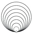
Figure 8. $(i):{\mathcal{G}}_{0,j-1}^{0,2j-2}$.

Figure 9. $(ii):{\mathcal{G}}_{1,j}^{2j-1,1}\subset{\mathcal{G}}_{1,j}$).

5.6. Balian-Bloch invariants at bouncing ball orbits of up-down symmetric domains

We now simplify the expression in Theorem 5.1 in the case of ${\mathbb{Z}}_{2}$-symmetric domains. The following result, stated in (9), is essentially a corollary of Theorem 5.1. It uses one simplification which will be proved in Proposition 6.5.

Corollary 5.11.

Suppose that $(\Omega,\gamma)$ is invariant under an isometric involution $\sigma$, and that $\gamma$ is a periodic $2$-link reflecting ray which is reversed by $\sigma.$ Then, modulo the error term $R_{2r}({\mathcal{J}}^{2j-2}f(0))$, $B_{\gamma^{r},j-1}$ is given by the expression (9).

Proof.

Using that $f_{-}=-f_{+}$, we can cancel the signs in the formula of Theorem 5.1 and add the top and bottom to obtain,

$$\begin{array}[]{lll}B_{\gamma^{r},j-1}&\equiv&4rL\;{\mathcal{A}}_{0}(r)\;\{(w_{{\mathcal{G}}_{1,j}^{2j,0}})\;\sum_{p=1}^{2r}(h^{pp})^{j}f^{(2j)}(0)\\ &&\\ &+&\;4\sum_{q,p=1}^{2r}[(w_{{\mathcal{G}}_{2,j+1}^{2j-1,3,0}})(h^{pp})^{j-1}h^{pq}h^{qq}\\ &&\\ &+&4(w_{\hat{{\mathcal{G}}}_{2,j+1}^{2j-1,3,0}})(h^{pp})^{j-2}(h^{pq})^{3}]\}f^{(3)}(0)f^{(2j-1)}(0).\end{array}$$

Further, in this ${\mathbb{Z}}_{2}$-symmetric case, all of the coefficients $h^{pp}$ are clearly equal. The sum $\sum_{q=1}^{2r}h^{pq}$ is independent of $p$ and is evaluated in Proposition (6.5), leaving the stated expression. ∎

6. Proof of Theorem (1.1)

We now prove the inverse spectral result for simply connected analytic plane domains with one special symmetry that reverses the endpoints of a bouncing ball orbit. The method is to recover the Taylor coefficients of the boundary defining function from the Balian-Bloch invariants at this orbit.

As simple warm-up for the proof, we give a new proof that centrally symmetric convex analytic domains whose shortest orbit is the unique orbit of its length (up to time-reversal) are spectrally determined within that class:

Proof of Corollary 1.2: Consider the wave invariants of the shortest orbit as given in Theorem 5.1. They are spectral invariants since the shortest length is a spectral invariant. By Ghomi’s theorem [Gh], the shortest orbit is a bouncing ball orbit. The orbit must be invariant under the two symmetries up to time-reversal since its length is of multiplicity one. Hence, the two symmetries imply that $f_{+}=-f_{-}:=f$ and that $f^{(2j+1)}(0)=0$ for all $j$. It follows that $f^{(2j)}(0)$ are spectral invariants for each $j$, and thus the domain is determined. QED

The same proof shows that simply connected analytic domains with the symmetry of an ellipse and with one axis of prescribed length $L$ are spectrally determined in that class.

6.1. Completion of the proof of Theorem 1.1

We now complete the proof of Theorem 1.1. Thus, we assume that $(\Omega,\gamma)$ is up-down symmetric, i.e. is invariant under an isometric involution $\sigma$, and that $\gamma$ is a periodic $2$-link reflecting ray which is reversed by $\sigma.$

There are two overall steps in the proof. First, and foremost, we study the expressions in Corollary 5.11. The key point is that the Hessian of the length function is a circulant matrix in the symmetric case, and that allows us to analyze the Hessian sums which occur as coefficients in the Balian-Bloch wave invariants. In particular, we decouple even and odd derivatives using the behavior of the Hessian sums under iterates $\gamma^{r}$. After that, a simple inductive argument shows that all Taylor coefficients of $f_{+}$ may be determined from the Balian-Bloch invariants.

We now begin the analysis of the Hessian sums.

6.2. Circulant Hessian at ${\mathbb{Z}}_{2}$-symmetric bouncing ball orbits

In the case of ${\mathbb{Z}}_{2}$-symmetric domains in the sense of Theorem 1.1, $R_{A}=R_{B}:=R$ and

(68) $$\cos\alpha/2=2(1-\frac{L}{R})\;\;(\mbox{elliptic case}),\;\;\;\cosh\alpha/2=2(1-\frac{L}{R})\;\;(\mbox{hyperbolic case}).$$

We put:

(69) $$a=-2\cos\alpha/2\;\;(\mbox{elliptic case}),\;\;\;a=-2\cosh\alpha/2\;\;(\mbox{hyperbolic case}).$$

By 16 and Proposition 2.2, the Hessian of the Length function in Cartesian graph coordinates simplifies to:

(70) $$H_{2r}=\frac{-1}{L}\left\{\begin{array}[]{lllll}a&1&0&\dots&1\\ &&&&\\ 1&a&1&\dots&0\\ &&&&\\ 0&1&a&1&0\\ &&&&\\ 0&0&1&a&1\dots\\ &&&&\\ \dots&\dots&\dots&\dots&\dots\\ &&&&\\ 1&0&0&\dots&a\end{array}\right\}.$$

We observe that (70) is a symmetric circulant matrix (or simply circulant) of the form

(71) $$(-L)H_{2r}=C(a,1,0,\dots,0,1),$$

where a circulant is a matrix of the form (cf. [D])

(72) $$C(c_{1},c_{2},\dots,c_{n})=\left\{\begin{array}[]{llll}c_{1}&c_{2}&\dots&c_{n}\\ &&&\\ c_{n}&c_{1}&\dots&c_{n-1}\\ &&&\\ \dots&\dots&\dots&\dots\\ &&&\\ c_{2}&c_{3}&\dots&c_{1}\end{array}\right\}.$$

Circulants are diagonalized by the finite Fourier matrix $F$ of rank $n$ defined by

(73) $$F^{*}=n^{-1/2}\left\{\begin{array}[]{llll}1&1&\dots&1\\ &&&\\ 1&w&\dots&w^{n-1}\\ &&&\\ \dots&\dots&\dots&\dots\\ &&&\\ 1&w^{n-1}&\dots&w^{(n-1)(n-1)}\end{array}\right\},\;\;\;\;w=e^{\frac{2\pi i}{n}}$$

Here, $F^{*}=(\bar{F})^{T}=\bar{F}$ is the adjoint of $F$. By [D], Theorem 3.2.2, we have $C=F^{*}\Lambda F$ where

(74) $$\Lambda=\Lambda_{C}=\mbox{diag}\;(p_{C}(1),\dots,p_{C}(w^{n-1}),\;\;\mbox{with}\;\;p_{C}(z)=c_{1}+c_{2}z+\dots+c_{n}z^{n-1}.$$

Here, by diag we mean the diagonal matrix with the exhibited entries.

6.3. Diagonalizing $H_{2r}^{-1}$

Applying the above to $C=H_{2r}$:

Proposition 6.1.

We have:

$$\begin{array}[]{l}H_{2r}^{-1}=-L\;F^{*}(\mbox{diag}\;(\frac{1}{a+2},\dots,\frac{1}{a+2\cos\frac{(2r-1)\pi}{r})})F,\end{array}$$

where $a$ is defined in (69).

Proof.

We use the notation $p_{a,r}(z)$ for $p_{C}(z)$ in the case where $C=C(a,1,0,\dots,0,1)$. Thus,

(75) $$p_{C}(z):=p_{a,r}(z):=a+z+z^{2r-1}.$$

By (73) we have,

(76) $$H_{2r}=\frac{-1}{L}\;F^{*}\mbox{diag}\;(p_{a,r}(1),\dots,p_{a,r}(w^{2r-1}))F,\;\;\;\;\;(w=e^{\frac{i\pi}{r}}).$$

Since

(77) $$p_{a,r}(w^{k}):=a+w^{k}+w^{-k},\;\;(w=e^{\frac{i\pi}{r}})$$

we have

(78) $$H_{2r}=\frac{-1}{L}\;F^{*}\mbox{diag}\;(a+2,\dots,a+2\cos\frac{(2r-1)\pi}{r})F,$$

and inverting gives the statement. ∎

6.4. Matrix elements of $H_{2r}^{-1}$ at a ${\mathbb{Z}}_{2}$-symmetric bouncing ball orbit

We will need explicit formulae for the matrix elements $h^{pq}_{2r}$ of $H_{2r}^{-1}$. The diagonalization of $H_{2r}^{-1}$ above gives one kind of formula. We also consider a second approach to inverting $H_{2r}$ (due to [K]) via finite difference equations. The two approaches give quite different formulae for the inverse Hessian sums and have different applications in the inverse results. In several of the calculations in this section, we assume for simplicity of exposition that $\gamma$ is elliptic; the hyperbolic case is easier and all formulae analytically continue from the elliptic to the hyperbolic cases.

For our purposes it will suffice to know the formulae for the elements $h^{1q}_{2r}.$ To emphasize the fact that the matrix elements depend on, and only on, $(r,a)$ we denote them by $h^{pq}_{2r}(a)$. The first formula comes directly from the diagonalization above.

Proposition 6.2.

With the above notation, we have

$$h^{1q}_{2r}(a)=\;\frac{-L}{2r}\sum_{k=0}^{2r-1}\frac{w^{(q-1)k}}{p_{a,r}(w^{k})},\;\;\;\;(w=e^{\frac{i\pi}{r}})$$

where the denominators are defined in (75)-(77).

The second, finite difference, approach expresses the inverse Hessian matrix elements $h_{2r}^{pq}$ in terms of Chebychev polynomials $T_{n},$ resp. $U_{n}$, of the first, resp. second, kind. They are defined by:

$$T_{n}(\cos\theta)=\cos n\theta,\;\;\;\;\;U_{n}(\cos\theta)=\frac{\sin(n+1)\theta}{\sin\theta}.$$

Proposition 6.3.

[K] (p. 190) With the above notation,

$$\begin{array}[]{l}(-L)^{-1}h^{pq}_{2r}(a)=\frac{1}{2[1-T_{2r}(-a/2)]}[U_{2r-q+p-1}(-a/2)+U_{q-p-1}(-a/2)],\;\;\;\;1\leq p\leq q\leq 2r)\end{array}$$

We note that $h^{pq}=h^{qp}$ so this formula determines all of the matrix elements.

The special cases $r=1,2$ are already very helpful in the inverse problem. We recall that

$$\begin{array}[]{l}T_{1}(x)=x,\;T_{2}(x)=2x^{2}-1,\;T_{3}(x)=4x^{3}-3x,\;T_{4}(x)=8x^{4}-8x^{2}+1;\\ \\ U_{1}(x)=2x,\;U_{2}(x)=4x^{2}-1,\;U_{3}(x)=8x^{3}-4x,\;U_{4}=16x^{2}-12x^{2}+1,\end{array}$$

from which we calculate:

(79) $$H_{2}^{-1}=\frac{-L}{a^{2}-4}\begin{pmatrix}a&-2\\ &\\ -2&a\end{pmatrix},$$

and

(80) $$H_{4}^{-1}=\frac{-L}{a^{4}-4a^{2}}\begin{pmatrix}a^{3}-2a&-a^{2}&2a&-a^{2}\\ \\ -a^{2}&a^{3}-2a&-a^{2}&2a\\ \\ 2a&-a^{2}&a^{3}-2a&-a^{2}\\ \\ -a^{2}&2a&-a^{2}&a^{3}-2a\end{pmatrix}.$$

In terms of Floquet angles, we have (in the elliptic case),

(81) $$h_{2r}^{pq}=\frac{-L}{2[1-T_{2r}(\cos\alpha/2)]}[U_{2r-q+p-1}(-\cos\alpha/2)+U_{q-p-1}(-\cos\alpha/2)],\;\;\;(1\leq p\leq q\leq 2r)),$$

hence

(82) $$\begin{array}[]{l}(-L)^{-1}\;h_{2r}^{pq}=\left\{\begin{array}[]{ll}\frac{(-1)^{p-q}}{2[1-\cos r\alpha)]}[\frac{\sin(2r-q+p)\alpha/2}{\sin\alpha/2}+\frac{\sin(q-p)\alpha/2}{\sin\alpha/2}]&(1\leq p\leq q\leq 2r)\\ &\\ \frac{(-1)^{p-q}}{2[1-\cos r\alpha]}[\frac{\sin(2r-p+q)\alpha/2}{\sin\alpha/2}+\frac{\sin(p-q)\alpha/2}{\sin\alpha/2}]&(1\leq q\leq p\leq 2r)\end{array}\right.\end{array}$$

We note that the expression in Proposition (6.2) is the Fourier inversion formula for (82).

Corollary 6.4.

We have: $(-L)^{-1}\;h_{2r}^{11}=\frac{U_{2r-1}(-\frac{a}{2})}{2(1-T_{2r}(-\frac{a}{2}))}=\frac{\sin r\alpha}{2(1-\cos r\alpha)\sin\frac{\alpha}{2}}=\frac{1}{2\sin\frac{\alpha}{2}}\cot\frac{r\alpha}{2}.$

6.5. Linear sums

We now complete the proof of Corollary 5.11 by summing the matrix elements in the first row $[H_{2r}^{-1}]_{1}=(h^{11},\dots,h^{1(2r)})$ (or column) of the inverse. As a check on the notation and assumptions, we calculate it in two different ways:

Proposition 6.5.

Suppose that $\gamma$ is a ${\mathbb{Z}}_{2}$-symmetric bouncing ball orbit. Then, for any $p$, $\sum_{q=1}^{2r}h_{2r}^{pq}=\frac{-L}{a+2}=\frac{-L}{2-2\cos\alpha/2}$.

Proof.

Because $H_{2r}^{-1}$ is a circulant matrix, the column sum is the same for all columns. Hence we only need to consider the first column.

(i) By Proposition 6.2, we have

$$\begin{array}[]{l}\sum_{q=1}^{2r}h^{pq}_{2r}=\sum_{q=1}^{2r}h^{1q}_{2r}=\frac{-L}{2r}\sum_{q=1}^{2r}\sum_{k=0}^{2r-1}\frac{w^{(q-1)k}}{p_{a,r}(w^{k})}\\ \\ =(-L)\;\sum_{k=0}^{2r-1}\frac{\delta_{k0}}{p_{a,r}(w^{k})}=\frac{-L}{p_{a,r}(1)}=\frac{-L}{2+a}=\frac{-L}{2-2\cos\alpha/2}.\end{array}$$

(ii) Since $\sum_{q=1}^{2r}h^{1q}_{2r}=\sum_{q=1}^{2r}h^{pq}_{2r}$ for any $p=1,\dots,2r$, we can set $p=1$ in the sum over $q$ to obtain,

(83) $$1=\sum_{p,q=1}^{2r}h_{pq^{\prime}}h^{pq}=[\sum_{p=1}^{2r}h_{pq^{\prime}}][\sum_{q=1}^{2r}h^{pq}].$$

It then follows from (16) and Proposition (2.2) that $(-L)^{-1}\;\sum_{p=1}^{2r}h_{pq^{\prime}}=2+a=2-2\cos\alpha/2$.

∎

6.6. Decoupling Balian-Bloch invariants

Corollary (5.11) expresses $B_{\gamma^{r},j-1}$ in terms of inverse Hessian matrix elements. To prove Theorem 1.1, it is essential to show that we can separately determine the two terms

1. $(h^{11}_{2r}(a))^{2}\{2(w_{{\mathcal{G}}_{1,j}^{2j,0}})f^{(2j)}(0)+4\frac{(w_{{\mathcal{G}}_{2,j+1}^{2j-1,3,0}})}{2+a}f^{(3)}(0)f^{(2j-1)}(0)\},$

2. $4(w_{\hat{{\mathcal{G}}}_{2,j+1}^{2j-1,3,0}})\sum_{q=1}^{2r}(h^{1q}_{2r}(a))^{3}\}f^{(3)}(0)f^{(2j-1)}(0).$

To decouple the terms we prove that they have behave independently under iterates $r$ of the bouncing ball orbit. We use the simple observation:

Lemma 6.6.

Let $F_{3}(r,a)=\sum_{q=1}^{2r}(h^{1q}_{2r}(a))^{3}$. If $(h^{11}_{2r}(a))^{-2}F_{3}(r,a)$ is non-constant in $r=1,2,3,\dots$, then both terms (1)-(2) can be determined from their sum as $r$ ranges over ${\bf N}.$

Proof.

Put

$$A=\{2(w_{{\mathcal{G}}_{1,j}^{2j,0}})f^{(2j)}(0)+4\frac{(w_{{\mathcal{G}}_{2,j+1}^{2j-1,3,0}})}{2+a}f^{(3)}(0)f^{(2j-1)}(0)\},\;\;B=4(w_{\hat{{\mathcal{G}}}_{2,j+1}^{2j-1,3,0}})f^{(3)}(0)f^{(2j-1)}(0).$$

It is assumed that we know $(h^{11}_{2r}(a))^{2}A+F_{3}(r,a)B$ for all $r\in{\bf N}$. To determine $A,B$ it is clearly sufficient that the matrix

$$\left(\begin{array}[]{ll}(h^{11}_{2r}(a))^{2}&F_{3}(r,a)\\ &\\ (h^{11}_{2s}(a))^{2}&F_{3}(s,a)\end{array}\right)$$

is invertible for some integers $r\not=s$. But this says precisely that $(h^{11}_{2r}(a))^{-2}F_{3}(r,a)\not=(h^{11}_{2s}(a))^{-2}F_{3}(s,a)$ for some integers $r\not=s.$ ∎

6.7. Cubic Hessian sums

We now prove that $(h^{11}_{2r}(a))^{-2}F_{3}(r,a)$ is indeed non-constant for all but finitely many $a$.

Proposition 6.7.

The ‘bad’ set ${\mathcal{B}}$ of (10) consists of $\{0,-1,\pm 2\}.$

Proof.

We will give two different proofs of the finiteness of ${\mathcal{B}}$. In both, we consider the sets

$${\mathcal{B}}_{r,s}=\{a\in{\mathbb{R}}:(h^{11}_{2r}(a))^{-2}F_{3}(r,a)=(h^{11}_{2s}(a))^{-2}F_{3}(s,a)\}.$$

6.7.1. First proof of Proposition 6.7: Dedekind sums

The first is based on an explicit calculation of $F_{3}(r,a)$ as a Dedekind sum. It is not very efficient in bounding the cardinality of ${\mathcal{B}}_{r,s}$ but gives a clear proof that this set is finite.

Lemma 6.8.

We have :

$$F_{3}(r,a)=\frac{(-L)^{3}}{(2r)^{2}}\sum_{k_{1},k_{2}=0}^{2r-1}\frac{1}{(a+2\cos\frac{k_{1}\pi}{r})(a+2\cos\frac{k_{2}\pi}{r})(a+2\cos\frac{(k_{1}+k_{2})\pi}{r})}.$$

In the hyperbolic case, we obtain a similar result with $\cos$ replaced by $\cosh.$

Proof.

Using Proposition 6.2, we have (with $w=e^{\frac{\pi i}{r}}$, and $\equiv$ equal to congruence modulo $2r$),

(84) $$\begin{array}[]{l}(2r)^{3}\frac{-1}{L^{3}}\sum_{q=1}^{2r}(h^{1q}_{2r}(a))^{3}=\sum_{q=1}^{2r}\{\sum_{k=0}^{2r-1}\frac{w^{(q-1)k}}{p_{a,r}(w^{k})}\}^{3}\\ \\ =\sum_{q=1}^{2r}\{\sum_{k_{1},k_{2},k_{3}=0}^{2r-1}\frac{w^{(q-1)(k_{1}+k_{2}+k_{3})}}{p_{a,r}(w^{k_{1}})p_{a,r}(w^{k_{2}})p_{a,r}(w^{k_{3}})}\}\\ \\ =2r\sum_{0\leq k_{i}\leq 2r-1;k_{1}+k_{2}+k_{3}\equiv 0}\frac{1}{p_{a,r}(w^{k_{1}})p_{a,r}(w^{k_{2}})p_{a,r}(w^{k_{3}})}\\ \\ =2r\sum_{0\leq k_{i}\leq 2r-1;k_{1}+k_{2}+k_{3}\equiv 0}\frac{1}{(a+2\cos\frac{k_{1}\pi}{r})(a+2\cos\frac{k_{2}\pi}{r})(a+2\cos\frac{k_{3}\pi}{r})}\\ \\ =2r\sum_{k_{1},k_{2}=0}^{2r-1}\frac{1}{(a+2\cos\frac{k_{1}\pi}{r})(a+2\cos\frac{k_{2}\pi}{r})(a+2\cos\frac{(k_{1}+k_{2})\pi}{r})}.\end{array}$$

∎

We now complete the proof of Proposition 6.7. By Corollary 6.4, $(h_{2r}^{11}(a))^{-2}F_{3}(r,a)$ is the rational function $\left(\frac{U_{r-1}(-\frac{a}{2})}{2(1-T_{r}(-\frac{a}{2}))}\right)^{-2}F_{3}(r,a)$, where as above, $T_{n},U_{n}$ are the Chebychev polynomials.

We now observe that for $r\not=s$, $\left(\frac{U_{r-1}(-\frac{a}{2})}{2(1-T_{r}(-\frac{a}{2}))}\right)^{-2}F_{3}(r,a)$ and $\left(\frac{U_{s-1}(-\frac{a}{2})}{2(1-T_{s}(-\frac{a}{2}))}\right)^{-2}F_{3}(s,a)$ are independent rational functions. Indeed, the poles for given $r$ are the values $a=-2\cos\frac{\alpha}{2}$ where $\alpha=\frac{2\pi k}{r}$ for some $k=1,\dots,2r.$ Hence, there can exist only finitely many solutions of the equation

(85) $$\left(\frac{U_{r-1}(-\frac{a}{2})}{2(1-T_{r}(-\frac{a}{2}))}\right)^{-2}F_{3}(r,a)=\left(\frac{U_{s-1}(-\frac{a}{2})}{2(1-T_{s}(-\frac{a}{2}))}\right)^{-2}F_{3}(s,a)$$

for any $r\not=s$, i.e. ${\mathcal{B}}_{r,s}$ is finite.

∎

It is interesting to observe that the sums above are generalized Dedekind sum, i.e. the sum $\sum_{\zeta\in D_{r}}I_{3}(\zeta,z)$ of the function

$$I_{3}(x;z)=\frac{1}{(z+\cos x_{1})(z+\cos x_{2})(z+\cos(x_{1}+x_{2}))}$$

over the set $D_{2r}$ of $2r$th roots of unity $\frac{\pi k}{r}\mbox{mod}\;2\pi{\mathbb{Z}}^{2}$ with $k=(k_{1},k_{2})\in[0,2r-1]\times[0,2r-1]$ of the torus. The summand is is a continuous periodic function of $(x_{1},x_{2})\in[0,1]\times[0,1]$ for $z\notin[-1,1]$. In fact, $I_{3}(x,z)$ is also symmetric under inversion and reflection across the diagonal and the sum has additionally the form of a multiple Dedekind sum

$$s_{2}(1,1;2r)=\sum_{k_{1},k_{2}(\text{mod}\,2r)}f(k_{1},r)f(k_{2},r)f(k_{1}+k_{2},r)$$

of two variables in the sense of L. Carlitz [Ca], with $f(k,r)=\frac{1}{(z+\cos 2\pi k/r)}.$

We remark that under the non-degeneracy assumption that $\alpha/\pi\notin{\mathbb{Q}}$, $\cos\alpha/2$ is never a pole of $F_{3}(r,z)$ for any $r$. In the hyperbolic case, it is obvious that $\cosh\alpha$ is never a pole of $F_{3}(r,z)$.

6.7.2. Second proof: Explicit inversion of the Hessian

We now give a second (and quite elementary) method of determining ${\mathcal{B}}$ by simply using the formulae for $H_{2}^{-1}$ (79) and $H_{4}^{-1}$ (80). This calculation is due to the referee and to H. Hezari.

From the explicit formula for $H_{2}^{-1}$ we have:

$$\sum_{q=1}^{2}(h_{2}^{1q}(a))^{3}=\left(\frac{-L}{a^{2}-4}\right)^{3}(a^{3}-8).$$

Further, $h_{2}^{11}=\frac{-aL}{a^{2}-4}$. From the explicit formula for $H_{4}^{-1}$ we have

$$\sum_{q=1}^{4}(h_{4}^{1q}(a))^{3}=\left(\frac{-L}{a^{4}-4a^{2}}\right)^{3}(a^{9}-6a^{7}-2a^{6}+12a^{5}).$$

Further, $h_{4}^{11}=(-L)\frac{a^{3}-2a}{a^{4}-4a^{2}}.$

Thus, ${\mathcal{B}}_{1,2}$ is the set of solutions $a$ of the equation

$$\begin{array}[]{l}\frac{a^{3}-8}{(a^{2}-4)^{3}}\frac{(a^{2}-4)^{2}}{a^{2}}=\frac{(a^{4}-4a^{2})^{2}}{(a^{3}-2a)^{2}}\frac{a^{9}-6a^{7}-2a^{6}+12a^{5}}{(a^{4}-4a^{2})^{3}}\\ \\ \iff(a^{3}-2a)^{2}(a^{3}-8)=a^{9}-6a^{7}-2a^{6}+12a^{5}\end{array}$$

A little bit of cancellation reduces the equation to degree $6$. The distinct roots are $\{0,-1,2,-2\}$. QED

6.8. Final step in proof of Theorem 1.1: Inductive determination of Taylor coefficients

We now prove by induction that on $j$ that $f^{2j}(0),f^{(2j-1)}(0)$ are wave trace invariants, hence spectral invariants of the Laplacian among domains in ${\mathcal{D}}_{1,L}$.

It is clear for $j=1$ since $(1-Lf^{(2)}(0)=\cos\alpha/2$ (resp. $\cosh\alpha/2$) and $\alpha$ is a Balian-Bloch (wave trace) invariant at $\gamma$ (see [Fr]). In the case $j=2$, the Balian-Bloch invariants have the form (9). Using that $\alpha$ is a Balian-Bloch invariant and the decoupling argument of Lemma 6.6 and Proposition 6.7, $(f^{(3)}(0))^{2}$ is a spectral invariant. By reflecting the domain across the bouncing ball axis if necessary, we may assume with no loss of generality that $f^{(3)}(0)>0$, and we have then determined $(f^{(3)}(0))$ from the sequence of Balian-Bloch invariants. Using again that $\alpha$ is determined by the Balian-Bloch invariants, it follows that $f^{(4)}(0)$ is determined.

We now carry forward the argument by induction. As $j\to j+1$, we may assume that ${\mathcal{J}}^{2j-2}f(0)$ is known. The terms denoted $R_{2r}{\mathcal{J}}^{2j-2}f(0)$ in Theorem 5.1 are universal polynomials in the data ${\mathcal{J}}^{2j-2}f(0)$, hence are also known. Thus, it suffices to determine $f^{(2j)}(0),f^{(2j-1)}(0)$ from (9). By the decoupling argument, we can determine $(f^{(3)}(0))(f^{(2j-1)}(0))$, hence $(f^{(2j-1)}(0))$, as long as $(f^{(3)}(0))\not=0.$ But then we can determine $f^{(2j)}(0).$ By induction, $f$ is determined and hence the domain.

This completes the proof of Theorem (1.1). QED

Remark 6.9.

From this argument it is only necessary that the coefficients $w_{{{\mathcal{G}}}}$ etc. are non-zero and universal. It is not necessary to know the precise values of the coefficients of $f^{(2j)}(0),f^{(2j-1)}(0)$.

6.9. The case where $f^{(3)}(0)=0$

If $f^{(3)}(0)=0$, the inductive argument clearly breaks down. There is a natural analogue of it as long as $f^{(5)}(0)\not=0$. We only sketch the analogue to make it seem plausible, but do not provide a complete proof.

Instead of inductively determining $f^{(2j)}(0),f^{(2j-1)}(0)$, we inductively determine $f^{(2j)}(0),f^{(2j-3)}(0)$ by a similar argument. Since $f^{(3)}(0)=0$, the terms $f^{(2j-1)}(0)$ have zero coefficients, and each new ‘odd’ term as $j\to j+1$ now has the form $[\sum_{q=1}^{r}(h^{pq})^{5}]f^{(5)}(0)f^{(2j-3)}(0)$. To carry out the analogue of the previous argument, it suffices to show that $h_{2r}^{-1}[\sum_{q=1}^{r}(h^{pq})^{5}]$ is a non-constant function of $r$. It should be plausible that this is the case, at least if we exclude a finite number of values of the Floquet exponents.

There then arises an infinite sequence of further sub-cases where all odd derivatives vanish up to some $j_{0}+1.$ To handle this case, we would need to show that $h_{2r}^{-1}[\sum_{q=1}^{r}(h^{pq})^{2j_{0}+1}]$ is non-constant for all $j_{0}$. This should again be plausible.

In the case where all odd derivatives vanish, the function $f_{+}$ is even and the proof reduces to the previously established case of two symmetries.

7. Proof of Theorem (1.4)

We now generalize the results from a bouncing ball orbit to iterates of a primitive $D_{m}$-invariant $m$-link reflecting ray $\gamma$. For short, we call $\gamma$ a $D_{m}$-ray.

7.1. Structure of coefficients at a $D_{m}$-ray

7.1.1. $D_{m}$-rays

In the dihedral case, we orient $\Omega$ so that the center of the dihedral action is $(0,0)$ and so that one vertex $v_{0}$ of $\gamma$ lies on the $y$-axis. We again define a small strip $T_{\epsilon}(\gamma)$, which intersects the boundary in $n$ arcs. We label the one through $v_{0}$ by $\alpha$. We then write $\alpha$ as the graph $y=f(x)$ of a function defined on a small interval around $(0,0)$ on the horizontal axis. Since we are only considering $D_{n}$-invariant rays, the domain is entirely determined by $\alpha$ and $f$.

We first need to choose a convenient parametrization of $\partial\Omega\cap T_{\epsilon}(\gamma).$ Either a polar parametrization or a Cartesian parametrization would do. For ease of comparison to the bouncing ball case, we prefer the Cartesian one. Thus, we use the parametrization $x\in(-\epsilon,\epsilon)\to(x,f(x))$ for the $\alpha$ piece. We then use $x\to R_{2\pi/m}^{j}(x,f(x))$ for the rotate $R_{2\pi/m}^{j}\alpha.$ When considering $\gamma^{r}$, we need variables $x_{js}(j=1,\dots,m;s=1,\dots,r),x_{js}\to R_{2\pi/m}^{j}(x_{js},x_{js}).$ We have:

$$\begin{array}[]{l}R_{2\pi/m}^{\sigma(p)}(x_{p},f(x_{p}))=(x_{p}^{\sigma(p)},(f(x_{p}))^{\sigma(p)})\\ \\ :=(\cos(2p\pi/m)x_{p}+\sin(2p\pi/m)f(x_{p}),-\sin(2p\pi/m)x_{p}+\cos(2p\pi/m)f(x_{p})).\end{array}$$

We also put $(-1,f^{\prime}(x_{p}))^{\sigma(p)}:=R_{2\pi/m}^{\sigma(p)}(-1,f^{\prime}(x_{p})).$

We then define the length functional

(86) $$\begin{array}[]{ll}{\mathcal{L}}^{\sigma}(y,x_{0},x_{1},\dots,x_{mr})&=|(x_{0},y)-(x_{1},f(x_{1}))^{\sigma(1)}|+|(x_{0},y)-(x_{rm},f(x_{rm}))^{\sigma(rm)}|\\ &\\ &+\sum_{p=1}^{mr-1}|(x_{p},f(x_{p}))^{\sigma(p)}-(x_{p+1},f(x_{p+1}))^{\sigma(p+1)}|\end{array}$$

We will need a formula for its Hessian in the case of a $D_{m}$-ray. By ([KT], Proposition 3), the Hessian $H_{rm}$ in $x-y$ coordinates at the critical point $(x_{1},\dots,x_{rm})$ corresponding to $\gamma^{r}$ is given by the matrix (2.2) with $s=\frac{2L}{R\sin\vartheta}$.

A key point in what follows (as in [Z1, Z2]) is that the reflection symmetry of $\alpha$ and $f$ implies that $f^{(2j-1)}(0)=0$ for all $j$. This eliminates the most serious obstacle to recovering $f$ from the wave trace invariants at $\gamma^{r}$, namely the fact that in the transition from the $j$th Balian-Bloch invariant to the $(j+1)$st, two new derivatives of $f$ appear.

As in the ${\mathbb{Z}}_{2}$-symmetric case, there are principal and non-principal terms. The principal term in the $D_{m}$ case, analogously to the bouncing ball case, equals $Tr\rho*N_{1}^{mr}\circ N_{1}^{\prime}(k)\circ\chi(k)$ for $r$ repetitions of the dihedrally symmetric orbit.

In analogy to Lemma (5.1) we prove:

Lemma 7.1.

Let $\gamma$ be a $D_{m}$- ray, and let $\rho$ be a smooth cutoff to $t=rL_{\gamma}$ as above. Then:

• $B_{\gamma^{r},j}=p_{m,r,j}(f^{(2)}(0),f^{(3)}(0),\cdots,f^{(2j+2)}(0))$ where $p_{2,r,j}(\xi_{1},\dots,\xi_{2j})$ is a polynomial. It is homogeneous of degree $-j$ under the dilation $f\to\lambda f,$ is invariant under the substitution $f(x)\to f(-x)$, and has degree $j+1$ in the Floquet data $e^{i\alpha r}.$

• In the expansion in Theorem (1.1) of [Z5] of $TrR_{\rho}((k+i\tau))$, $f^{(2j)}(0)$ appears first in the $k^{-j+1}$st order term, and then only in the $k^{-j+1}$st order term in the stationary phase expansion of the principal term $Tr\rho*N_{1}^{mr}\circ N_{1}^{\prime}(k)\circ\chi(k)$;

• This coefficient has the form

  $$\begin{array}[]{l}B_{\gamma^{r},j-1}=mr(h^{11})^{j}f^{(2j)}(0)+R_{mr}({\mathcal{J}}^{2j-2}f(0)),\end{array}$$

  where the remainder $R_{mr}({\mathcal{J}}^{2j-2}f(0))$ is a polynomial in the designated jet of $f.$

Proof of Lemma (7.1)

We use the analogue of Theorem 3.1 for the case of the dihedral ray. As in the case of a bouncing ball orbit, we have a finite number of oscillatory integrals $I_{M\rho}^{\sigma,w}$ arising from the regularization of the trace. We express the resulting oscillatory integrals in Cartesian coordinates of (polar coordinates are also convenient for this calculation). We put $x=(x_{0},y_{0})$. Each oscillatory integral $I_{M,\rho}^{\sigma,w}$ localizes at critical points, we may insert a cutoff to $T_{\epsilon}(\gamma).$ This gives $m^{M}$ possible terms, corresponding to the possible choices of the arcs in the product $(\partial\Omega\cap T_{\epsilon}(\gamma))^{M}.$ We put:

$$\{m^{M}\}:=\{\sigma:{\mathbb{Z}}_{M}\to\{1,\dots,m\}\},$$

and write

$$\begin{array}[]{l}R_{2\pi/m}^{\sigma(p)}(x_{p},f(x_{p}))=(x_{p}^{\sigma(p)},(f(x_{p}))^{\sigma(p)})\\ \\ :=(\cos(2p\pi/m)x_{p}+\sin(2p\pi/m)f(x_{p}),-\sin(2p\pi/m)x_{p}+\cos(2p\pi/m)f(x_{p})).\end{array}$$

We also put $(-1,f^{\prime}(x_{p}))^{\sigma(p)}:=R_{2\pi/m}^{\sigma(p)}(-1,f^{\prime}(x_{p})).$

The oscillatory integrals have the phase functions ${\mathcal{L}}^{\sigma}$ on $(\partial\Omega\cap T_{\epsilon}(\gamma))^{rm}$ of the form:

(87) $${\mathcal{L}}^{\sigma}(x_{1},\dots,x_{mr})=\sum_{p=1}^{mr-1}|(x_{p},f(x_{p}))^{\sigma(p)}-(x_{p+1},f(x_{p+1}))^{\sigma(p+1)}|$$

Only $2m$ $\sigma$’s ( $2$ modulo cyclic permutations) give length functions which have critical points with critical value $rL_{\gamma},$ namely the ones $\sigma_{0}$ where $\sigma_{0}(n)=R(\pm n2\pi/m)$. Indeed, the only Snell polygon with this length is $\gamma^{r}$ by assumption, and so $(x_{1}^{\sigma(1)},\dots,x_{rm}^{\sigma(rm)})$ must correspond to the vertices of $\gamma^{\pm r}$. Since the good length functions represent isometric situations, it suffices to consider the case $\sigma_{0}(n)=R(n2\pi/m)$. In this case, we denote the length function simply by $L$ and to simplify the notation we drop the subscript in $\sigma_{0}.$

We now make a stationary phase analysis as in the bouncing ball case to obtain the expressions in Theorem (5.1). As mentioned above, there are two principal terms: The principal oscillatory integrals $I_{rm,\rho}^{\sigma_{0},w_{\pm}}$ are those in which $M=rm$ and in which no factors of $N_{0}$ occur, i.e. $\sigma_{0}(j)=1$ for all $j=1,\dots,rm$. Also, there are now $m$ components of the boundary at the reflection points, and $w_{\pm}$ cycles around them for $r$ iterates.

7.2. The principal terms

They have the phase

(88) $${\mathcal{L}}^{\sigma}(x_{1},\dots,x_{mr})=\sum_{j=1}^{mr-1}\sqrt{(x_{j+1}^{\sigma(j+1)}-x_{j}^{\sigma(j)})^{2}+(f(x_{j+1})^{\sigma(j+1)}-(f(x_{j}))^{\sigma(j)})^{2}},$$

and the amplitude

(89) $$\begin{array}[]{l}a^{0}(k,x_{1},\dots,x_{mr},y)=\Pi_{p=1}^{m}a_{1}((k+i\tau)\sqrt{(x_{p-1}^{\sigma(p-1)}-(x_{p}^{\sigma(p)})^{2}+(f(x_{p-1})^{\sigma(p-1)}-f(x_{p})^{\sigma(p)})^{2}})\\ \\ \frac{(x_{p-1}^{\sigma(p-1)},,f(x_{p-1})^{\sigma(p-1)})-(x_{p}^{\sigma(p)},f(x_{p})^{\sigma(p)})\cdot\nu_{x_{p}^{\sigma(p)},f(x_{p})^{\sigma(p)}}}{\sqrt{(x_{p-1}^{\sigma(p-1)}-x_{p}^{\sigma(p)})^{2}+(f(x_{p-1})^{\sigma(p-1)}-f(x_{p})^{\sigma(p)})^{2}}}\end{array}$$

We observe that it has the form ${\mathcal{A}}(x,y,f,f^{\prime}).$ The $f^{\prime}$ dependence will be particularly important later on.

7.2.1. The principal term: The data $f^{2j}(0)$

As in the bouncing ball case, by the same argument, the data $f^{(2j)}(0)$ appears first in the term of order $k^{-j+1}$ and it appears linearly in the term $a^{0}{\mathcal{H}}^{j}R_{3}.$ We now show that its coefficient is given by the formula in Lemma (7.1). Due to symmetry, it suffices to consider any axis and one endpoint of it. We observe that only the ‘diagonal terms’ of ${\mathcal{H}}^{j}$, i.e. those involving only derivatives in a single variable $\frac{\partial}{\partial x_{k}}$, can produce the factor $f^{(2j)}(0)$. Since $f^{\prime}(0)=x|_{x=0}=0$ and since the angle between successive links and the normal equals $\pi/m$ an examination of (45) shows that the coefficient of $f^{(2j)}(0)$ equals

$$\begin{array}[]{l}\sum_{p=1}^{rm}(h^{pp})^{j}(\frac{\partial}{\partial x_{p}})^{2j}{\mathcal{L}}^{\sigma}(y;x_{0},\dots,x_{k},\dots x_{mr})=[\sum_{p=1}^{mr}(h^{pp})^{j}]f^{(2j)}(0).\end{array}$$

The data $f^{(2j-1)}(0)$ vanishes due to the symmetry around each dihedral axis.

Finally, as in the bouncing ball case, and for the same reasons, non-principal oscillatory integrals do not contribute to this data.

This completes the proof of Lemma (7.1). ∎

Remark It would also be natural to employ polar coordinates in the proof. In that case, we align $\Omega$ so that one of the reflection axes is the positive $x$-axis, and express $\partial\Omega$ parametrically in the form $r=r(\vartheta)$ where $\vartheta$ is the angle to the $x$-axis. Then $r(-\vartheta)=r(\vartheta),r(\vartheta+\frac{2\pi j}{m})=r(\vartheta).$ The goal then is to determine $r$. To do so, we write out that $q(\vartheta)=(r(\vartheta)\cos(\vartheta),r(\vartheta)\sin(\vartheta)$ and compute as above. We find that $r^{(2j)}(0)$ arises first in the $k^{-1+j}$ term with the same coefficient as for $f^{(2j)}(0)$ above. The rest of the proof proceeds as with Cartesian coordinates.

7.3. Dihedral domains: Proof of Theorem (1.4)

We now complete the proof of Theorem (1.4).

We prove by induction on $j$ that $f^{2j}(0)$ is a Balian-Bloch invariant. It is clear for $j=1$ since $(1-Lf^{(2)}(0)=\cos(h)\alpha/2$ and $\alpha$ is a Balian-Bloch (wave trace) invariant at $\gamma$. In general, the eigenvalues of $P_{\gamma}$ are wave trace invariants [F].

Assuming the result for $n<j-1$, it follows that $p^{sub}_{r,n-1}$ is a spectral invariant. It thus suffices to extract $f^{2j}(0)$ from $p^{0}_{r,j-1}$, i.e. from $\{\sum_{p=1}^{2r}(h^{pp})^{j}\}f^{(2j)}(0).$

Thus, the only missing step is to show that if $\gamma$ is $D_{m}$-ray, then the $h^{pp}$ are Balian-Bloch invariants of $\gamma^{r}$. In other words, that $s$ is a wave trace invariant. If $\lambda,\lambda^{-1}$ denote the eigenvalues of $P_{\gamma^{r}}$, then we have $\lambda+\lambda^{-1}=2+\det H_{mr}.$ Here we use that all $b_{j}$ equal $1$. It follows that $s$ is a function of $\lambda$, hence that it is a Balian-Bloch invariant.

The proof of Theorem (1.4) is complete.

References

- [A] S. Axelrod, Overview and warmup example for perturbation theory with instantons. Geometry and physics (Aarhus, 1995), 321–338, Lecture Notes in Pure and Appl. Math., 184, Dekker, New York, 1997.
- [AG] D. Alonso and P. Gaspard, expansion for the periodic orbit quantization of chaotic systems. Chaos 3 (1993), no. 4, 601–612.
- [B] R. Bacher (unpublished note, 2002).
- [BB1] R. Balian and C. Bloch, Distribution of eigenfrequencies for the wave equation in a finite domain I: three-dimensional problem with smooth boundary surface, Ann. Phys. 60 (1970), 401-447.
- [BB2] R. Balian and C. Bloch, Distribution of eigenfrequencies for the wave equation in a finite domain. III. Eigenfrequency density oscillations. Ann. Physics 69 (1972), 76–160.
- [Bu] B. Burmeister, Korrekturen zur Gutzwillerschen Spurformel fuer Quantenbillards, Diplomarbeit am II. Institut fuer Theoretische Physik der Universitat Hamburg (1995).
- [Ca] L. Carlitz, Many-term relations for multiple Dedekind sums. Indian J. Math. 20 (1978), 77–89.
- [C] G. Carron, Déterminant relatif et la fonction Xi. Amer. J. Math. 124 (2002), no. 2, 307–352.
- [CV] Y.Colin de Verdière, Sur les longuers des trajectoires periodiques d’un billard, In: P.Dazord and N. Desolneux-Moulis (eds.) Geometrie Symplectique et de Contact: Autour du Theoreme de Poincare-Birkhoff. Travaux en Cours, Sem. Sud-Rhodanien de Geometrie III Pairs: Herman (1984), 122-139.
- [D] P.J. Davis, Circulant Matrices, Wiley-Insterscience, New York (1979).
- [EP] Eckmann, J.-P.; Pillet, C.-A. Zeta functions with Dirichlet and Neumann boundary conditions for exterior domains. Papers honouring the 60th birthday of Klaus Hepp and of Walter Hunziker, Part II (Zürich, 1995). Helv. Phys. Acta 70 (1997), no. 1-2, 44–65.
- [E] P. Etingof, Lecture Notes on Quantum Field Theory (MIT OpenCourseWare).
- [F] G. Folland, Introduction to Partial Differential Equations, Princeton Math. Notes, Princeton U. Press (1976).
- [Fr] D. Fried, Cyclic resultants of reciprocal polynomials. Holomorphic dynamics (Mexico, 1986), 124–128, Lecture Notes in Math., 1345, Springer, Berlin-New York (1988).
- [Gh] M. Ghomi, Shortest periodic billiard trajectories in convex bodies, Geom. Funct. Anal. Volume 14, Number 2, 295 - 302.
- [GWW1] C. Gordon, D.L. Webb and S. Wolpert, Isospectral plane domains and surfaces via Riemannian orbifolds. Invent. Math. 110 (1992), no. 1, 1–22
- [G] V. Guillemin, Wave-trace invariants. Duke Math. J. 83 (1996), no. 2, 287–352.
- [GM] V.Guillemin and R.B.Melrose, The Poisson summation formula for manifolds with boundary, Adv.in Math. 32 (1979), 204 - 232.
- [HZ] A. Hassell and S. Zelditch, Quantum ergodicity and boundary values of eigenfunctions, Comm. Math. Phys. 248 (2004), 119-168.
- [Hö] L. Hörmander, The Analysis of Linear Partial Differential Operators, Volumes I–IV, Springer-Verlag Berlin Heidelberg, 1983.
- [ISZ] A. Iantchenko, J. Sjöstrand, and M. Zworski, Birkhoff normal forms in semi-classical inverse problems. Math. Res. Lett. 9 (2002), no. 2-3, 337–362.
- [K] D. Kershaw, The explicit inverses of two commonly occurring matrices. Math. Comp. 23 (1969), 189–191.
- [KT] V.V. Kozlov and D. V. Treshchev, Billiards: A Genetic Introduction to the Dynamics of Systems with Impacts, Translations of Math. Monographs 89, AMS publications, Providence, R.I. (1991).
- [M] V.A. Marchenko, Sturm-Liouville operators and applications. Translated from the Russian by A. Iacob. Operator Theory: Advances and Applications, 22. Birkh user Verlag, Basel, 1986.
- [MM1] S. Marvizi and R. B. Melrose, Spectral invariants of convex planar regions. J. Differential Geom. 17 (1982), no. 3, 475–502.
- [PS] V.M.Petkov and L.N.Stoyanov, Geometry of Reflecting Rays and Inverse Spectral Problems, John Wiley and Sons, N.Y. (1992).
- [SZ] J. Sjöstrand and M. Zworski, Quantum monodromy and semi-classical trace formulae. J. Math. Pures Appl. 81 (2002), 1–33.
- [T] M.E. Taylor, Partial Differential Equations , I- II, Appl. Math.Sci. 115 -116, Springer-Verlag (1996).
- [V] A. Vasy, Propagation of singularities for the wave equation on manifolds with corners, Inverse Problems 20:1349-1354 (2004).
- [Z1] S. Zelditch, Spectral determination of analytic bi-axisymmetric plane domains (announcement). Math. Res. Lett. 6 (1999), 457–464.
- [Z2] S. Zelditch, Spectral determination of analytic bi-axisymmetric plane domains, Geom. Funct. Anal. 10 (2000), no. 3, 628–677.
- [Z3] S. Zelditch, The inverse spectral problem for surfaces of revolution, Journal of Differential Geometry 49 (1998), 207-264.
- [Z4] S. Zelditch, Inverse resonance problem for symmetric analytic obstacles in the plane, IMA Volume 137: Geometric Methods in Inverse Problems and PDE Control. C.B. Croke, I. Lasiecka, G. Uhlmann, and M. S.Vogelius eds.
- [Z5] S. Zelditch, Inverse spectral problem for analytic plane domains I: Balian-Bloch trace formula, Comm. Math. Phys. 248 (2004), 357-407.