Tight contact structures on fibered hyperbolic 3-manifolds

Abstract.

We take a first step towards understanding the relationship between foliations and universally tight contact structures on hyperbolic 3-manifolds. If a surface bundle over a circle has pseudo-Anosov holonomy, we obtain a classification of “extremal” tight contact structures. Specifically, there is exactly one contact structure whose Euler class, when evaluated on the fiber, equals the Euler number of the fiber. This rigidity theorem is a consequence of properties of the action of pseudo-Anosov maps on the complex of curves of the fiber and a remarkable flexibility property of convex surfaces in such a space. Indeed this flexibility may be seen in surface bundles over an interval where the analogous classification theorem is also established.

Recent work of Colin [4] and the authors [18], and work in progress of Colin, Giroux, and the first author [5] combine to suggest a very general, but rough, classification principle for universally tight contact structures.

Principle: If $M$ is a closed, oriented, irreducible 3-manifold, then $M$ carries finitely many (isotopy classes of) universally tight contact structures if and only if $M$ is atoroidal.

The work [5] on the finiteness of tight contact structures does not give an accurate bound on the number of universally tight contact structures carried by an atoroidal manifold. (For example, it does not address the existence question.) Indeed, it is not clear, a priori, just what are the properties of a 3-manifold which determine the number and nature of the tight contact structures it carries.

As a first step towards understanding the classification of tight contact structures for atoroidal manifolds with infinite fundamental group, we consider hyperbolic 3-manifolds which fiber over the circle. These manifolds have enough structure to be accessible through a variety of techniques, and the relationships between the various structures they support are often extremely good predictors of similar relationships in more general 3-manifolds. The uniqueness theorem (Theorem 0.2) suggests that contact topology may ultimately be a discrete version of foliation theory. More specifically, Eliashberg and Thurston [7] showed that any taut foliation may be perturbed to a universally tight contact structure. There are many foliations of a fibered hyperbolic manifold that contain a fixed fiber as a leaf, yet perturbing any of them always produces the same universally tight contact structure by Theorem 0.2.

Contact structures on fibered hyperbolic 3-manifolds are studied by splitting the manifold along a fiber and later recreating the original manifold by gluing back using the pseudo-Anosov monodromy map. This leads to an analysis of tight contact structures on the product $\Sigma\times[0,1]$, where $\Sigma$ is a closed, oriented surface of genus $g>1$. There is a surprisingly small number of (isotopy classes of) tight contact structures on $\Sigma\times I$ with boundary conditions given in Theorem 0.1, and the theory for $g>1$ is quite different from the $g=1$ case treated in [11, 14]. Much of the classification on $\Sigma\times I$, at least in the cases we are led to study, can be encoded in the curve complex on $\Sigma$. Therefore, Theorem 0.2 exploits the interplay between the pseudo-Anosov monodromy and the curve complex of $\Sigma$. The fact that there are only a few distinct isotopy classes of tight contact structures on $\Sigma\times I$ (of the kind we are interested in) is in large part due to a remarkable flexibility property (Proposition 5.2) enjoyed by surfaces in $\Sigma\times I$ which are isotopic to $\Sigma\times\{t\}$. To paraphrase the result, by isotoping such a surface, we are free to choose any pair of parallel, nonseparating curves as its dividing set.

Let $\Sigma$ be a closed, oriented surface of genus $g>1$. We study tight contact structures $\xi$ on the 3-manifold $M=\Sigma\times I=\Sigma\times[0,1]$ which satisfy the following condition:

Extremal condition. $\langle e(\xi),\Sigma_{t}\rangle=\pm(2g-2)$, $t\in[0,1]$, where the left-hand side refers to the Euler class of $\xi$ evaluated on $\Sigma_{t}$.

Here we write $\Sigma_{t}=\Sigma\times\{t\}$. Tight contact structures on $\Sigma\times I$ satisfying this condition are said to be extremal for the following reason: if $\xi$ is a tight contact structure on $\Sigma\times I$, then the Bennequin inequality [1, 6] states that:

$$-(2g-2)\leq\langle e(\xi),\Sigma_{t}\rangle\leq 2g-2.$$

One of the main results of this paper is the following classification:

Theorem 0.1.

Let $\Sigma$ be a closed oriented surface of genus $\geq 2$ and $M=\Sigma\times I$. Fix dividing sets $\Gamma_{\Sigma_{i}}=2\gamma_{i}$ (2 parallel disjoint copies of $\gamma_{i}$), $i=0,1$, so that $\gamma_{0}$, $\gamma_{1}$ are nonseparating curves and $\chi((\Sigma_{0})_{+})-\chi((\Sigma_{0})_{-})=\chi((\Sigma_{1})_{+})-\chi((\Sigma_{1})_{-})$, where $(\Sigma_{i})_{+}$, $(\Sigma_{i})_{-}$ are the positive and negative regions of $\Sigma_{i}\setminus\Gamma_{\Sigma_{i}}$. Then choose a characteristic foliation $\mathcal{F}$ on $\partial M$ which is adapted to $\Gamma_{\Sigma_{0}}\sqcup\Gamma_{\Sigma_{1}}$. We have the following:

1. All the tight contact structures which satisfy the boundary condition $\mathcal{F}$ are universally tight.

2. If $\gamma_{0}\not=\gamma_{1}$, then $\#\pi_{0}(Tight(M,\mathcal{F}))=4$. Provided $\gamma_{0}$ and $\gamma_{1}$ are not homologous, they are distinguished by the relative Euler classes $PD(\tilde{e}(\xi))=\pm\gamma_{0}\pm\gamma_{1}$.

3. If $\gamma_{0}=\gamma_{1}$, then $\#\pi_{0}(Tight(M,\mathcal{F}))=5$. Three of them (one of them $I$-invariant) have relative Euler class $PD(\tilde{e}(\xi))=0$ and the other two have $PD(\tilde{e}(\xi))=\pm 2\gamma_{0}=\pm 2\gamma_{1}$.

Here, $\#\pi_{0}(Tight(M,\mathcal{F}))$ denotes the number of connected components of tight contact 2-plane fields adapted to $\mathcal{F}$, and the relative Euler class is an invariant of the tight contact structure which will be defined in Section 3. Theorem 0.1 is a complete classification in the extremal case, provided $\#\Gamma_{\Sigma_{i}}=2$ and $\Gamma_{\Sigma_{i}}$ consists of two nonseparating curves. The proof of Theorem 0.1, given in Section 5 requires one involved calculation, found in Section 4, followed by judicious use of general facts from curve complex theory, found in Section 2.

The extremal case is currently the only case we understand, but we also have the following theorem:

Theorem 0.2.

Let $M$ be a closed, oriented, hyperbolic 3-manifold which fibers over $S^{1}$, where the fiber is a closed oriented surface $\Sigma$ of genus $g>1$ and the monodromy map is pseudo-Anosov. Then there exists a unique tight contact structure in each of the two extremal cases, i.e., $\langle e(\xi),\Sigma\rangle=\pm(2g-2)$. This contact structure is universally tight and weakly symplectically fillable. Moreover, every $C^{0}$-small perturbation of the fibration into a contact structure is isotopic to the unique extremal tight contact structure.

Perturbing the fibration by $\Sigma$ into a contact structure is either done directly or by appealing to the perturbation result of Eliashberg and Thurston [7], which also tells us that the contact structure is weakly symplectically semi-fillable. It is interesting to note that, no matter how we perturb the fibration into a contact structure, the resulting tight contact structure is the same. This contrasts with the case where the fiber is a torus [10].

In this paper we adopt the following conventions:

1. The ambient manifold $M$ is an oriented, compact $3$-manifold.

2. $\xi$ = positive contact structure which is co-oriented by a global 1-form $\alpha$.

3. A convex surface $\Sigma$ is either closed or compact with Legendrian boundary.

4. $\Gamma_{\Sigma}$ = dividing multicurve of a convex surface $\Sigma$.

5. $\#\Gamma_{\Sigma}$ = number of connected components of $\Gamma_{\Sigma}$.

6. $\Sigma\setminus\Gamma_{\Sigma}=\Sigma_{+}\cup\Sigma_{-}$, where $\Sigma_{+}$ (resp. $\Sigma_{-}$) is the region where the normal orientation of $\Sigma$ is the same as (resp. opposite to) the normal orientation for $\xi$.

7. $|\beta\cap\gamma|$ = geometric intersection number of two curves $\beta$ and $\gamma$ on a surface.

8. $\#(\beta\cap\gamma)$ = cardinality of the intersection.

9. $\Sigma\setminus\gamma$ = metric closure of the complement of $\gamma$ in $\Sigma$.

10. $t(\beta,Fr_{S})$ = twisting number of a Legendrian curve with respect to the framing induced from the surface $S$.

1. Tools from convex surface theory

In this section we collect some results from the theory of convex surfaces which are nonstandard. For standard results on convex surfaces, we refer the reader to [9, 12, 14, 17, 18].

We first recall the Legendrian realization principle (LeRP), in a slightly stronger form. An embedded graph $C$ on a convex surface $\Sigma$ is nonisolating if (1) $C$ is transverse to $\Gamma_{\Sigma}$, (2) the univalent vertices of $C$ lie on $\Gamma_{\Sigma}$, (3) all the other vertices do not lie on $\Gamma_{\Sigma}$, and (4) every component of $\Sigma\backslash(\Gamma_{\Sigma}\cup C)$ has a boundary component which intersects $\Gamma_{\Sigma}$.

Theorem 1.1 (Legendrian realization).

Let $C$ be a nonisolating graph on a convex surface $\Sigma$ and $v$ a contact vector field transverse to $\Sigma$. Then there exists an isotopy $\phi_{s}$, $s\in[0,1]$ so that:

1. $\phi_{0}=id$, $\phi_{s}|_{\Gamma_{\Sigma}}=id$.

2. $\phi_{s}(\Sigma)\pitchfork v$ (and hence $\phi_{s}(\Sigma)$ are all convex),

3. $\phi_{1}(\Gamma_{\Sigma})=\Gamma_{\phi_{1}(\Sigma)}$,

4. $\phi_{1}(C)$ is Legendrian.

Proposition 1.2 (The Right-to-Life Principle).

Let $S$ be a convex surface in a tight contact manifold $(M,\xi)$ and let $\delta$ be a Legendrian arc transverse to $\Gamma_{S}$ with endpoints on $\Gamma_{S}$, for which $|\Gamma_{S}\cap\delta|=3$. Suppose an “abstract bypass move” was applied to $\Gamma_{S}$ along $\delta$ and yielded a dividing set isotopic to $\Gamma_{S}$, i.e., this move was trivial. (Here, by an “abstract bypass move” we simply mean a modification of the multicurve $\Gamma_{S}\subset S$ which would theoretically arise from attaching a bypass along $\delta$ — there may or may not be an actual bypass half-disk along $\delta$ inside the ambient 3-manifold.) Then there exists an actual bypass half-disk $B$ along $\delta$ (from the proper side) contained in the $I$-invariant neighborhood of $S$.

The Right-to-Life Principle is a consequence of Eliashberg’s classification of tight contact structures on the 3-ball [6], and is proved in Lemma 1.8 of [16]. Here we recreate the proof.

Proof.

Suppose $\delta$ intersects $\Gamma_{S}$ successively along $p_{1},p_{2},p_{3}$. Since $\delta$ gives rise to a trivial “abstract bypass move”, we may assume that the subarc from $p_{1}$ to $p_{2}$, together with a subarc of $\Gamma_{S}$, bounds a disk $D^{\prime}$. Let $D\subset S$ be a disk which contains $D^{\prime}\cup\delta$. We may assume $\partial D$ is Legendrian with $tb(\partial D)=-2$ — to do this we apply LeRP (or Giroux’s Flexibility Theorem [9, 14]) to $\partial D$, while fixing $\delta$. Then $\Gamma_{D}$ consists of two arcs $\gamma_{1}\ni p_{1},p_{2}$ and $\gamma_{2}\ni p_{3}$.

We will now find the actual bypass along $\delta\times\{0\}$ inside the $I$-invariant tight contact structure on $D\times[0,1]$. (Here we are assuming that the bypass attached from the $D\times[0,1]$-direction is the trivial bypass.) Let $p_{0}$ be a point on $\gamma_{2}$ ($\not=p_{3}$) for which there exists a Legendrian arc $\delta^{\prime}\subset D$ from $p_{1}$ to $p_{0}$ which does not intersect $\Gamma_{D}$ except at endpoints and does not intersect $\delta$ except at $p_{1}$. Define $\delta_{0}=\delta\cup\delta^{\prime}$ and $\delta_{1}\subset D$ to be a Legendrian arc from $p_{3}$ to $p_{0}$ that lies on the same side of $\gamma_{2}$ as $\delta_{0}$ and has no other intersections with $\Gamma_{D}$. Now consider an arc $\varepsilon\subset D$ from $p_{0}$ to $p_{3}$ that lies on the opposite side of $\gamma_{2}$ as $\delta_{0}$ and $\delta_{1}$ and has no other intersections with $\Gamma_{D}$. Let $A\subset D\times[0,1]$ be a convex annulus such that $\partial A=(\delta_{0}\cup\varepsilon)\times\{0\}\cup(\delta_{1}\cup\varepsilon)\times\{1\}$ and such that $(\varepsilon\times[0,1])\subset A$. Since $\Gamma_{\varepsilon\times I}$ consists of an arc $\{q\}\times[0,1]$ ($q\in\varepsilon$), $\Gamma_{A}$ must contain one of two possible bypasses, one intersecting $\{p_{0},p_{1},p_{2}\}\times\{0\}$ and the other intersecting $\{p_{1},p_{2},p_{3}\}\times\{0\}$. The former is a bypass which cannot exist since it gives rise to an overtwisted disk. Therefore we obtain the second, as stated in the proposition. ∎

Lemma 1.3 (Bypass Sliding Lemma).

Let $R$ be an embedded rectangle with consecutive sides $a,b,c,d$ in a convex surface $S$ such that $a$ is an arc of attachment of a bypass, $b$ and $d$ are subsets of $\Gamma_{S}$ and $c$ is a Legendrian arc which is efficient (rel endpoints) with respect to $\Gamma_{S}$. Then there exists a bypass for which $c$ is its arc of attachment.

Proof.

The appendix to [15] explains how to explicitly move the endpoints of the Legendrian arc of attachment. In this paper, we will deduce the Bypass Sliding Lemma from the Right-to-Life Principle.

Let $R^{\prime}\supset R$ be an embedded disk in $S$ satisfying the following:

• $\partial R^{\prime}$ is Legendrian, $\partial R^{\prime}\pitchfork\Gamma_{S}$, and $tb(\partial R^{\prime})=-3$.

• $\partial R^{\prime}=a^{\prime}\cup b^{\prime}\cup c^{\prime}\cup d^{\prime}$, where $a^{\prime}$ and $c^{\prime}$ are Legendrian arcs parallel to and close to $a$ and $c$, respectively. The four arcs $a^{\prime},b^{\prime},c^{\prime},d^{\prime}$ are consecutive sides of a rectangle whose corners, lying on $\Gamma_{S}$, have been smoothed.

• $\Gamma_{R^{\prime}}$ consists of three parallel (= nested) dividing arcs.

Such an $R^{\prime}$ exists by LeRP. Suppose we attach the bypass along $a$ to obtain a convex surface $R^{\prime\prime}$ isotopic to $R^{\prime}$ rel boundary. Note that, away from $a$, $R^{\prime\prime}$ and $R^{\prime}$ are identical. Now, the “abstract bypass move” along $c$ applied to $R^{\prime\prime}$ still yields the same dividing set $\Gamma_{R^{\prime\prime}}$. Therefore, the bypass must also exist along $c$. (In fact, it exists in a small neighborhood of $R^{\prime\prime}$.) ∎

Lemma 1.4.

Let $S$ be a closed convex surface of genus $g$ and $\Gamma_{S}$ its dividing set, consisting of one homotopically nontrivial separating curve. Let $S\times I$ be its $I$-invariant neighborhood. Then there exists a bypass in $S\times I$ along $S\times\{1\}$ such that the dividing set $\Gamma_{S^{\prime}}$ of the surface $S^{\prime}$, obtained after bypass attachment, consists of three curves parallel to $\Gamma_{S}$. Moreover, the arc of attachment $\alpha$ is contained in an annular neighborhood of $\Gamma_{S}$ and intersects $\Gamma_{S}$ in 3 points, and the two half disks bounded by $\alpha$ and $\Gamma_{S}$ have a common intersection along an arc contained in $\Gamma_{S}$.

For a more thorough discussion on dividing-curve increasing bypasses, see [16].

Remarks.

1. Typically, we increase $\#\Gamma$ by folding along a Legendrian divide (see [14] or [18]). This generates a pair of dividing curves parallel to the Legendrian divide. However, this folding operation to increase $\#\Gamma$ does not occur immediately for free, in case the curve we want to realize as a Legendrian divide is an isolating curve for $\Gamma$ in the sense of LeRP. This is the case in Lemma 1.4.

2. Lemma 1.4 can be viewed as a strengthened form of LeRP and of Giroux’s Flexibility Theorem.

3. Lemma 1.4 (or the proof therein) shows that folds along homotopically nontrivial closed curves always exist.

Proof.

In order to use LeRP, we first cut along some annulus $\gamma^{*}\times I$, where $\gamma^{*}\subset S$ is a closed nonseparating curve which does not intersect $\Gamma_{S}$. Let $N$ be $(S\times I)\setminus(\gamma^{*}\times I)$, with edges rounded near $\gamma^{*}\times I$, so that $\partial N$ is convex. We will write $G=\partial N$. Note that we may think of $\Gamma_{S}$ as a sub-multicurve of $\Gamma_{G}$. A parallel copy $(\Gamma_{S})^{*}$ of $\Gamma_{S}$ on $G$, pushed off closer towards $\gamma^{*}\times I$ and disjoint from $\Gamma_{S}$, is then nonisolating. We can then use LeRP to realize $(\Gamma_{S})^{*}$ as a Legendrian divide and use it to perform a fold. (For more details on folding and bypasses, see [18]. In a standard $I$-invariant neighborhood of $G$, we therefore find a parallel copy $G^{\prime}$, where $\Gamma_{G^{\prime}}$ is $\Gamma_{G}$, with 2 parallel curves (parallel to $\Gamma_{S}$) added. To get from $G^{\prime}$ to $G$, a bypass $B$ is attached along $G^{\prime}$ which straddles the three distinct dividing curves parallel to $\Gamma_{S}$. This has the effect of reducing $\#\Gamma$ by $2$. Every bypass operation always has its inverse operation, and the inverse of $B$ is $B^{-1}$, which is attached along $G$ and increases $\#\Gamma$ by $2$. We can now view $B^{-1}$ as also attached onto $S$ and intersecting $\Gamma_{S}$ three times. The Legendrian arc of attachment for $G$ may not exist on $S$, but one can always find an appropriate arc of attachment using Giroux’s Flexibility Theorem. (Remark: The arc of attachment does not really matter here — the only thing that really matters is the twisting number of the bypass Legendrian arc.) Hence the bypass survives passage from being a bypass for $\Gamma_{G}$ to being a bypass for $\Gamma_{S}$. ∎

2. Tools from Curve Complex Theory

In this section, we recall several facts from the theory of curve complexes which will become useful later. Let $\Sigma$ be a closed oriented surface of genus $g\geq 2$ — we stress here that all the lemmas and propositions of this section require $g\geq 2$. Let $\mathcal{C}(\Sigma)$ be the curve complex for $\Sigma$. The vertices of $\mathcal{C}(\Sigma)$ consist of isotopy classes of homotopically nontrivial closed curves on $\Sigma$ and there is a single edge between each pair $\gamma_{0}$, $\gamma_{1}$ of (isotopy classes of) closed curves with $|\gamma_{0}\cap\gamma_{1}|=0$. Note that we do not attach simplices of higher dimension, since they are not needed. The facts we need from the theory of curve complexes are variations and strengthenings of the basic Lemma 2.1 below. We refer the reader to [19] for an exposition on curve complexes, an extensive reference, and a proof of Lemma 2.1.

Lemma 2.1.

$\mathcal{C}(\Sigma)$ is connected, i.e., given two closed curves $\alpha$, $\alpha^{\prime}$ in $\mathcal{C}(\Sigma)$, there exists a sequence $\alpha_{0}=\alpha,\alpha_{1},\dots,\alpha_{k}=\alpha^{\prime}$ in $\mathcal{C}(\Sigma)$ where $|\alpha_{i-1}\cap\alpha_{i}|=0$, $i=1,\dots,k$.

Alternatively, we have the following:

Lemma 2.2.

Given two nonseparating closed curves $\alpha$, $\alpha^{\prime}$ on $\Sigma$, there exists a sequence $\alpha_{0}=\alpha,\alpha_{1},\dots,\alpha_{k}=\alpha^{\prime}$ of closed curves where $|\alpha_{i-1}\cap\alpha_{i}|=1$, $i=1,\dots,k$.

Proposition 2.3.

Given two nonseparating closed curves $\alpha$ and $\alpha^{\prime}$ on $\Sigma$, there exists a sequence $\alpha_{0}=\alpha,\alpha_{1},\dots,\alpha_{k}=\alpha^{\prime}$ of closed curves where:

1. $\alpha_{i}$ are nonseparating, $i=0,\dots,k$.

2. $|\alpha_{i-1}\cap\alpha_{i}|=0$, $i=1,\dots,k$.

3. $\alpha_{i-1}$ and $\alpha_{i}$ are not homologically equivalent, $i=1,\dots,k$.

Proof.

By Lemma 2.2, there is a sequence $\alpha_{0}=\alpha,\alpha_{1},\dots,\alpha_{k}=\alpha^{\prime}$ of closed curves where $|\alpha_{i-1}\cap\alpha_{i}|=1$, $i=1,\dots,k$. A neighborhood $U_{i-1}$ of $\alpha_{i-1}\cup\alpha_{i}$ is a punctured torus. Since the genus of $\Sigma$ is at least 2, $\Sigma-U_{i-1}$ contains a nonseparating curve $\beta_{i-1}$. Therefore, $\alpha_{0},\beta_{0},\alpha_{1},\beta_{1},\dots,\alpha_{k}$ is the desired sequence. ∎

Proposition 2.4.

Given three nonseparating closed curves $\alpha$, $\beta$, $\beta^{\prime}$ on $\Sigma$, where $|\alpha\cap\beta|=0$, $|\alpha\cap\beta^{\prime}|=0$, $\alpha$ and $\beta$ are nonhomologous, and $\alpha$ and $\beta^{\prime}$ are nonhomologous, there exists a sequence $\beta_{0}=\beta,\beta_{1},\dots,\beta_{k}=\beta^{\prime}$ of closed curves where:

1. $\beta_{i}$ are nonseparating, $i=0,\dots,k$.

2. $|\alpha\cap\beta_{i}|=0$, $i=0,\dots,k$.

3. $|\beta_{i-1}\cap\beta_{i}|=1$, $i=1,\dots,k$.

Proof.

By assumption $\Sigma\setminus\alpha$ is connected. If $\gamma$ is a curve in $\Sigma$ such that $|\gamma\cap\alpha|=0$, then $\gamma$ is nonseparating and not homologous to $\alpha$ if and only if $\gamma$ is nonseparating as a subset of $\Sigma\setminus\alpha$. Let $\Sigma^{\prime}$ be $\Sigma\setminus\alpha$ together with two disks capping off the boundary components corresponding to $\alpha$. Then $\beta$ and $\beta^{\prime}$ are nonseparating closed curves of $\Sigma^{\prime}$ and applying Lemma 2.2 to $\beta,\beta^{\prime}$ and $\Sigma^{\prime}$ produces the desired sequence of curves. ∎

Proposition 2.5.

Given two nonseparating closed curves $\alpha$ and $\alpha^{\prime}$ on $\Sigma$, there exists a sequence $\alpha_{0}=\alpha,\alpha_{1},\dots,\alpha_{k}=\alpha^{\prime}$ of closed curves where:

1. $\alpha_{i}$ are nonseparating, $i=0,\dots k$.

2. $|\alpha_{i-1}\cap\alpha_{i}|=1$, $i=1,\dots,k$.

3. $|\alpha_{i-1}\cap\alpha_{i+1}|=0$, $i=1,\dots,k-1$.

Proof.

Let $\alpha_{0}=\alpha,\alpha_{1},\dots,\alpha_{k}=\alpha^{\prime}$ be a sequence for which $|\alpha_{i-1}\cap\alpha_{i}|=1$, $i=1,\dots,k$, as guaranteed by Lemma 2.2. Suppose that $j\geq 1$ is the smallest integer for which $|\alpha_{j-1}\cap\alpha_{j+1}|>0$. We show how to insert curves into the sequence between $\alpha_{j}$ and $\alpha_{j+1}$, until Condition 3 is satisfied, at least up to $\alpha_{j+1}$. Since curves are only inserted after $\alpha_{j}$, there is no danger that Condition 3 will be disturbed for earlier terms in the sequence.

For notational convenience, we shall take $j=1$. We will always assume that $\alpha_{0}\cap\alpha_{1}$ is not an element of $\alpha_{2}$. Suppose that $|\alpha_{0}\cap\alpha_{2}|\geq 1$. The following cases are used to inductively decrease the number of intersections between $\alpha_{0}$ and $\alpha_{2}$.

Case 1: Not all intersections between $\alpha_{0}$ and $\alpha_{2}$ have the same sign.

Then there exist two points $p,q\in\alpha_{0}\cap\alpha_{2}$ with opposite signs of intersection, and an arc $[p,q]_{\alpha_{0}}\subset\alpha_{0}$ which connects $p$ and $q$ such that $[p,q]_{\alpha_{0}}$ does not intersect $\alpha_{1}$ and contains no point of $\alpha_{2}$ in its interior. Cut-and-paste surgery of $\alpha_{2}$ along $[p,q]_{\alpha_{0}}$ produces two curves; let $\beta$ the component which intersects $\alpha_{1}$ once. The sequence $\alpha_{0},\alpha_{1},\beta,\alpha_{1},\alpha_{2}$ satisfies Condition 2 (and hence Condition 1), and is closer to satisfying Condition 3 than the original sequence, in the sense that the total number of intersection points of type $\alpha_{i-1}\cap\alpha_{i+1}$ has been reduced. Here it is understood that the second $\alpha_{1}$ in the sequence is slightly isotoped off the first $\alpha_{1}$ so that the two curves are disjoint as required in Condition 3.

Case 2: All intersections of $\alpha_{0}$ and $\alpha_{2}$ have the same sign and $|\alpha_{0}\cap\alpha_{2}|\geq 2$.

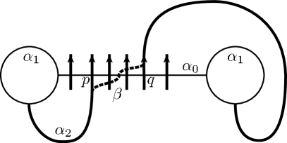
Figure 1. Case 2

Let $[p,q]_{\alpha_{2}}$, $p,q\in\alpha_{0}\cap\alpha_{2}$, be the smallest interval in $\alpha_{2}$ that contains $\alpha_{1}\cap\alpha_{2}$. Let $[p,q]_{\alpha_{0}}$ be the interval in $\alpha_{0}$ (with endpoints $p,q$) which does not intersect $\alpha_{1}$. Let $\beta=[p,q]_{\alpha_{2}}\cup[p,q]_{\alpha_{0}}$. After a slight isotopy of $\beta$, the sequence $\alpha_{0},\alpha_{1},\beta,\alpha_{1},\alpha_{2}$ satisfies Condition 2. Condition 3 is not satisfied, but at least the first and third terms of this interim sequence intersect only once and $|\beta\cap\alpha_{2}|<|\alpha_{0}\cap\alpha_{2}|$.

Case 3: $|\alpha_{0}\cap\alpha_{2}|=1$.

Let $U$ be a regular neighborhood of $\alpha_{0}\cup\alpha_{1}\cup\alpha_{2}$ in $\Sigma$. Let $V=U\setminus(\alpha_{0}\cup\alpha_{1})$. $V$ is a planar surface with 4 boundary components, one corresponding to $\alpha_{0}\cup\alpha_{1}$, shown as a rectangle in Figure 2, and three others denoted $A,B$ and $C$. The construction of the desired sequence of curves depends on the relation of $A,B$ and $C$ to the rest of $\Sigma$. In each of the following cases, $S$ will denote a connected subsurface of $\Sigma$ which satisfies $\partial S\subset A\cup B\cup C$ and whose interior $int(S)$ is disjoint from $V$.

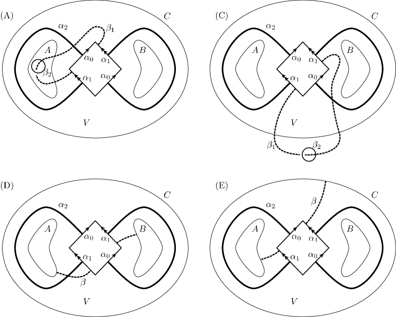
Figure 2. Case 3

(A) $A\subset S$ and $\text{genus}(S)\geq 1$. Choose $\beta_{1}$ as indicated in Figure 2(A), that is, $\beta_{1}$ starts on $\alpha_{1}$, then passes across $A$ into $S$ and back to $A$ without separating $S$, and then crosses $\alpha_{2}$ before returning to the point it started from, but from the opposite side of $\alpha_{1}$. Let $\beta_{2}\subset S$ be a curve such that $|\beta_{2}\cap\beta_{1}|=1$. The sequence $\alpha_{0},\alpha_{1},\beta_{1},\beta_{2},\beta_{1},\alpha_{2}$ satisfies Conditions 1–3.

(B) $B\subset S$ and $\text{genus}(S)\geq 1$. This is similar to (A).

(C) $C\subset S$ and $\text{genus}(S)\geq 1$. Choose $\beta_{1}$ and $\beta_{2}$ as shown in Figure 2(C) and the sequence $\alpha_{0},\alpha_{1},\beta_{1},\beta_{2},\beta_{1},\alpha_{2}$ will satisfy Conditions 1–3.

(D) $A\cup B\subset S$. Choose an arc in $V$ that runs from $A$, across $\alpha_{2}$ and $\alpha_{1}$ and then to $B$. Complete this arc to a curve $\beta$ by attaching an arc in $S$. The sequence $\alpha_{0},\alpha_{1},\beta,A,\beta,\alpha_{2}$ satisfies Conditions 1–3.

(E) $A\cup C\subset S$. Choose an arc in $V$ that runs from $C$, across $\alpha_{1}$ and then to $A$. Complete this arc to a curve $\beta$ by attaching an arc in $S$. The sequence $\alpha_{0},\alpha_{1},\beta,\alpha_{1},\alpha_{2}$ satisfies Conditions 1–3.

(F) $B\cup C\subset S$. This is similar to (E).

The only possibility not covered in (A)–(F) is if each of $A,B$ and $C$ bound disks, but this would imply $\text{genus}(\Sigma)=1$, contrary to assumption. ∎

3. Definition of the relative Euler class

Let $M=\Sigma\times I=\Sigma\times[0,1]$ and $\Sigma_{t}=\Sigma\times\{t\}$. If $\Sigma_{t}$ is convex, we denote $\Gamma_{t}=\Gamma_{\Sigma_{t}}$. Let $\xi$ be a tight contact structure on $M$ which satisfies $\langle e(\xi),\Sigma_{t}\rangle=\pm(2g-2)$. Since the situation is symmetric under sign change, we will additionally assume that $\langle e(\xi),\Sigma_{t}\rangle=-(2g-2)$.

First recall the following identity (cf. Kanda [21] or Eliashberg [6]):

(1) $$\langle e(\xi),S\rangle=\chi(S_{+})-\chi(S_{-}).$$

Here $S$ is a closed convex surface.

According to Giroux’s criterion [12], a closed convex surface $\Sigma\not=S^{2}$ has a tight neighborhood if and only if no connected component of $\Sigma_{\pm}$ is a disk. This implies that $\chi(\Sigma_{\pm})\leq 0$. Hence, the extremal condition implies that $\chi(\Sigma_{+})=-(2g-2)$ and $\chi(\Sigma_{-})=0$. In other words, $\Sigma_{-}$ is a nonempty union of annuli. Here, recall that both $\Sigma_{+}$ and $\Sigma_{-}$ of a convex surface $\Sigma$ are nonempty, since there must be both sources ($\Sigma_{+}$) and sinks ($\Sigma_{-}$) for the characteristic foliation.

This section is devoted to defining the relative Euler class $\tilde{e}(\xi)$ of $\xi$, not to be confused with the Euler class $e(\xi)$ used previously. It is sufficient to define the relative Euler class on annuli, as follows. Let $\gamma\subset\Sigma$ be a closed curve. Suppose first that $\gamma\times\{0,1\}$ is efficient with respect to $\partial M$, i.e., intersects $\Gamma_{\partial M}$ minimally in its isotopy class in $\partial M$. If $\gamma\times\{0,1\}$ is nonisolating in $\partial M$ (which is the case for example when $\gamma$ is nonseparating in $\Sigma$), then we may use the Legendrian realization principle (LeRP) [14] to make $\gamma\times\{0,1\}$ Legendrian. If $S=\gamma\times I\subset M$ is a convex surface, then we define:

(2) $$\langle\tilde{e}(\xi),S\rangle=\chi(S_{+})-\chi(S_{-}).$$

In general, choose $\gamma\times\{0,1\}$ (i.e., introduce extra intersections with $\Gamma_{\partial M}$) so that the following condition holds:

$\gamma\times\{0,1\}$ is nonisolating and every connected component of $(\gamma\times\{i\})\cap(\Sigma_{i})_{-}$, $i=0,1$, is a nonseparating arc.

If this condition is satisfied, we will say that $\gamma\times\{0,1\}$ has been primped. We remark here that (i) $(\Sigma_{i})_{-}$ is a union of annuli, and (ii) components of $(\gamma\times\{i\})\cap(\Sigma_{i})_{+}$ may be separating. We take $S$ convex with primped $\partial S=\gamma\times\{0,1\}$ and define $\langle\tilde{e}(\xi),S\rangle$ as in Equation 2.

What we would like to prove is that $\tilde{e}(\xi)$ is indeed a homology invariant, i.e., lives in $H^{2}(M,\partial M;\mathbb{Z})$. This follows from the following three lemmas.

Lemma 3.1.

Let $S$ and $S^{\prime}$ be convex surfaces with $\partial S=\partial S^{\prime}$ primped Legendrian curves on $\partial M$. If $S$ and $S^{\prime}$ are isotopic rel boundary, then $\langle\tilde{e}(\xi),S\rangle=\langle\tilde{e}(\xi),S^{\prime}\rangle$.

Proof.

Since $\partial S=\partial S^{\prime}$, we consider $S\cup(-S^{\prime})$. After rounding along the common edge and perturbing slightly if necessary (without changing the isotopy class of the dividing set), we may take $S\cup(-S^{\prime})$ to be a closed immersed surface. Although Equation 1 holds for closed convex surfaces (convex surfaces are embedded by definition), we may clearly extend Kanda’s argument in [21] to immersed surfaces which have meaningful positive and negative regions. Therefore, we have:

$$\langle\tilde{e}(\xi),S\rangle-\langle\tilde{e}(\xi),S^{\prime}\rangle = [\chi(S_{+})-\chi(S_{-})]-[\chi(S_{+}^{\prime})-\chi(S_{-}^{\prime})]$$

$$= \chi(S_{+}\cup S^{\prime}_{-})-\chi(S_{-}\cup S^{\prime}_{+})$$

$$= \langle e(\xi),S\cup(-S^{\prime})\rangle=0.$$

This proves that $\langle\tilde{e}(\xi),S\rangle$ is independent of the choice of $S$, provided $\partial S$ is fixed. ∎

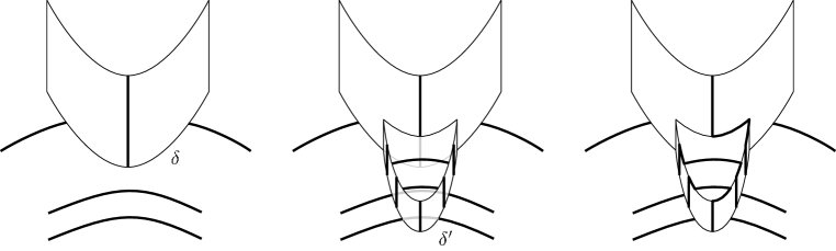
Figure 3. Isotopy of $\delta$ to $\delta^{\prime}$

Lemma 3.2.

Let $S=\delta\times I$ and $S^{\prime}=\delta^{\prime}\times I$ be isotopic convex surfaces with primped Legendrian boundary in $M$. Then $\langle\tilde{e}(\xi),S\rangle=\langle\tilde{e}(\xi),S^{\prime}\rangle$.

Proof.

The key point of using primped curves is that dividing curves of $\Sigma\times\{0,1\}$ (in the extremal case) come in pairs, and we can isotop one primped curve to another primped curve in the same isotopy class by pushing $\delta\times\{0,1\}$ across two curves in a pair simultaneously, i.e. by changing the annulus by a sequence of operations of the type described in Figure 3 (or its inverse). We see that such an isotopy changes the dividing set on the annulus by adding (or deleting) a nested pair of boundary compressible arcs. This amounts to adding (or removing) one disk region each for $S_{+}$ and $S_{-}$ and does not change $\langle\tilde{e}(\xi),S\rangle$. A finite sequence of such steps will bring us to the situation where we can apply the previous lemma. ∎

Next, we prove additivity.

Lemma 3.3.

Let $\delta_{i}$, $i=1,2$, be two oriented nonseparating curves on $\Sigma$ with nontrivial geometric intersection. Let $S_{i}=\delta_{i}\times I$ and form $S=S_{1}+S_{2}=\delta\times I$ by the natural cut-and-paste operation corresponding to homology addition. Then

$$\langle\tilde{e}(\xi),S\rangle=\langle\tilde{e}(\xi),S_{1}\rangle+\langle\tilde{e}(\xi),S_{2}\rangle.$$

Proof.

Consider the graph $C=\delta_{1}\cup\delta_{2}$, where $\delta_{1}\pitchfork\delta_{2}$ and $\delta_{1}\cap\delta_{2}$ does not intersect $\Gamma_{\Sigma}\cup\Sigma_{-}$. Assume enough extra intersections of $\Gamma_{\Sigma}\cap\delta_{i}$ have been introduced to $\delta_{i}$, $i=1,2$, so that $\delta_{i}$ is primped and $C$ satisfies the nonisolating condition. We may take the common intersections $\delta_{1}\cap\delta_{2}$ to be elliptic tangencies, using a slightly stronger version of LeRP which is easily derived from Giroux’s Flexibility Theorem [14], and $(\delta_{1}\cap\delta_{2})\times I$ to be transverse curves, by perturbing if necessary. Let $\delta^{\prime}=\delta_{1}+\delta_{2}$ be the multicurve obtained by smoothing the intersection $\delta_{1}\cap\delta_{2}$ in the standard manner. Then the surface $S^{\prime}$ obtained by performing a cut-and-paste along the transverse curve and smoothing the corners satisfies the following equality:

$$\langle\tilde{e}(\xi),S^{\prime}\rangle=\langle\tilde{e}(\xi),S_{1}\rangle+\langle\tilde{e}(\xi),S_{2}\rangle.$$

The equality follows from relating $\chi(S^{\prime}_{+})-\chi(S^{\prime}_{-})$ to the more standard way of computing $\langle\tilde{e}(\xi),S^{\prime}\rangle$ using signs and types of isolated singularities as in Kanda’s argument in [21]. Now, $\partial S^{\prime}$ is primped, since we took the intersections $\delta_{1}\cap\delta_{2}$ to be away from $\Sigma_{-}$. Therefore, Lemma 3.2 implies that $\langle\tilde{e}(\xi),S^{\prime}\rangle=\langle\tilde{e}(\xi),S\rangle$. ∎

We will usually express $\tilde{e}(\xi)\in H^{2}(M,\partial M;\mathbb{Z})$ in terms of its Poincaré dual $PD(\tilde{e}(\xi))\in H_{1}(M;\mathbb{Z})$.

4. Computation of the base case

Recall that, by our choice of $\langle e(\xi),\Sigma_{t}\rangle$, $(\Sigma_{i})_{-}$, $i=0,1$, is a union of annuli. If we assume that there is only one pair of dividing curves on each $\Sigma_{i}$, then $(\Sigma_{i})_{-}$ is an annulus and $(\Sigma_{i})_{+}$ is its complement in $\Sigma_{i}$ (i.e., “most” of the surface).

We will now consider the following special case, which turns out to be the most fundamental:

Base Case. $\Gamma_{i}=2\gamma_{i}$, $i=0,1$, and $|\gamma_{0}\cap\gamma_{1}|=1$.

Here, $k\gamma$ is shorthand for $k$ parallel (mutually nonintersecting) copies of a closed curve $\gamma$.

Theorem 4.1.

Let $\Sigma$ be a closed surface of genus $g\geq 2$, $M=\Sigma\times I$ the ambient manifold, and $\mathcal{F}$ a characteristic foliation on $\partial M$ adapted to $\Gamma_{0}\sqcup\Gamma_{1}$ of the Base Case. Let $Tight(M,\mathcal{F})$ be the space of tight contact 2-plane fields which induce $\mathcal{F}$ along $\partial M$. Then we have the following:

1. $\#\pi_{0}(Tight(M,\mathcal{F}))=4$ .

2. The isotopy classes of tight contact structures are distinguished by their relative Euler class, which are:

   $$PD(\tilde{e}(\xi))=\pm\gamma_{0}\pm\gamma_{1}\in H_{1}(M;\mathbb{Z}).$$

3. All the tight contact structures are universally tight.

This computation is a little involved, and occupies Sections 4.1 through 4.4. In what follows, when we prescribe a boundary condition for a 3-manifold $M$, we will simply give $\Gamma_{\partial M}$, although, strictly speaking, we need to also assign the characteristic foliation $\mathcal{F}$ on $\partial M$ adapted to $\Gamma_{\partial M}$. We will assume that some convenient characteristic foliation is prescribed, since the actual number of tight contact structures is independent of the actual characteristic foliation adapted to $\Gamma_{\partial M}$ (see [14]). The following is a preliminary lemma.

Lemma 4.2.

There exists a unique tight contact structure on $H=S\times I$, where $S$ is a compact oriented surface with nonempty boundary, $S_{0}$, $S_{1}$, and $(\partial S)\times I$ are convex, $\Gamma_{S_{0}}=\Gamma_{S_{1}}$ are $\partial$-parallel, and $\Gamma_{\partial S\times I}$ are vertical. (Here vertical means the dividing curves are arcs $\{pt\}\times I$.) This tight contact structure is universally tight, and is obtained by perturbing the foliation of $H$ by leaves $S\times\{t\}$, $t\in[0,1]$, into a contact structure.

Proof.

Observe that $H=S\times I$ is a handlebody and that $\Gamma_{\partial H}$, after edge-rounding [14], is isotopic to $\partial S\times\{{1\over 2}\}$. See Figure 4.

Figure 4. Dividing multicurve after edge-rounding.

Consider a meridional disk $D=\gamma\times I$, where $\gamma$ is a non-boundary-parallel, properly embedded arc on $S$. Then, after rounding, $\partial D$ intersects $\Gamma_{\partial H}$ along exactly two points. Make $\partial D$ Legendrian and $D$ convex. Then the Thurston-Bennequin invariant $tb(\partial D)$ equals $-1$, and there is a unique dividing curve configuration on $D$ consistent with this boundary condition. Moreover, there is a system of such meridional disks $D_{1},\dots,D_{k}$ which decompose $H$ into 3-balls $B^{3}$, each with $\Gamma_{\partial B^{3}}=S^{1}$. By Eliashberg’s uniqueness theorem for tight contact structures on the 3-ball (c.f. [6]), there is a unique tight contact structure up to isotopy rel boundary on each of the $B^{3}$’s. This implies that there exists at most one tight contact structure on $H$ with given $\Gamma_{\partial H}$. Now, to prove that there indeed exists a (universally) tight contact structure on $H$ with given $\Gamma_{\partial H}$, we glue back using Theorem 4.3 below. Note that $\Gamma_{D_{i}}$ is $\partial$-parallel on each meridional disk $D_{i}$. We leave the statement of the perturbation to the reader. ∎

Theorem 4.3 (Colin [3]).

Let $(M,\xi)$ be an oriented, compact, connected, irreducible, contact 3-manifold and $S\subset M$ an incompressible convex surface with nonempty Legendrian boundary and $\partial$-parallel dividing set $\Gamma_{S}$. If $(M\setminus S,\xi|_{M\setminus S})$ is universally tight, then $(M,\xi)$ is universally tight.

We now begin the analysis of the Base Case. Let us position the dividing curves $2\gamma_{0}$ and $2\gamma_{1}$ as in Figure 5, that is, we suppose $\#(\gamma_{0}\cap\gamma_{1})=1$ and we have oriented $\gamma_{0}$ and $\gamma_{1}$ so that the intersection pairing $\langle\gamma_{1},\gamma_{0}\rangle$ on $\Sigma$ equals $+1$. Now consider an oriented closed curve $\gamma$ which satisfies $\#(\gamma\cap\gamma_{i})=1$ and $\langle\gamma,\gamma_{i}\rangle=1$, $i=0,1$. For our convenience, we will assume that $\gamma_{0}$ and $\gamma_{1}$ are identical except in a thin annulus $\mathcal{A}$ parallel to but disjoint from $\gamma$, obtained as follows. First push $\gamma$ off of itself in the direction opposite the direction given by the orientation of $\gamma_{1}$ to obtain $\gamma^{\prime}$. Then let $\mathcal{A}$ be a small annular neighborhood of $\gamma^{\prime}$. $\gamma_{0}$ is then obtained from $\gamma_{1}$ via a Dehn twist in $\mathcal{A}$. We will write $\Gamma_{\Sigma_{1}}\cap\gamma=\{p_{1},p_{2}\}\times\{1\}$, $\Gamma_{\Sigma_{0}}\cap\gamma=\{p_{1},p_{2}\}\times\{0\}$. Our first cut of $M=\Sigma\times I$ will be along the convex surface $A=\gamma\times I$, where $A=\gamma\times I$ is given the orientation induced from $\gamma$ and $I$.

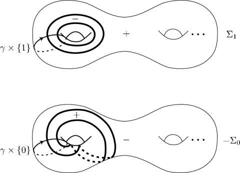
Figure 5. Suitable choice of $\Gamma_{0}$ and $\Gamma_{1}$.

There are two general classes of dividing curves $\Gamma_{A}$ which we denote by ${\mbox{\it I}}_{k}$ and $\mbox{\it II}_{n}^{\pm}$. The dividing set ${\mbox{\it I}}_{k}$ consists of 2 parallel nonseparating dividing curves (i.e., dividing curves which go across from $\gamma\times\{0\}$ to $\gamma\times\{1\}$). Here, $k\in\mathbb{Z}$ denotes the holonomy, or the amount of spiraling, defined as follows. First, zero holonomy $k=0$ means the dividing curves are vertical in the sense that they are isotopic rel boundary to $\{q_{1},q_{2}\}\times[0,1]$, where $\{q_{1},q_{2}\}\times\{0,1\}$ are the endpoints of $\Gamma_{A}$. The holonomy is $k$ if $\Gamma_{A}$ is obtained from $\{q_{1},q_{2}\}\times[0,1]$ by doing $k$ negative Dehn twists along the core curve of $A$. The dividing set $\mbox{\it II}_{n}^{+}$ (resp. $\mbox{\it II}_{n}^{-}$), $n\in\mathbb{Z}^{\geq 0}$, consists of two $\partial$-parallel dividing curves which split off half-disks, where the half-disk along $\gamma\times\{1\}$ is positive (resp. negative) and there are $n$ parallel homotopically essential closed curves. See Figure 6 for the possibilities.

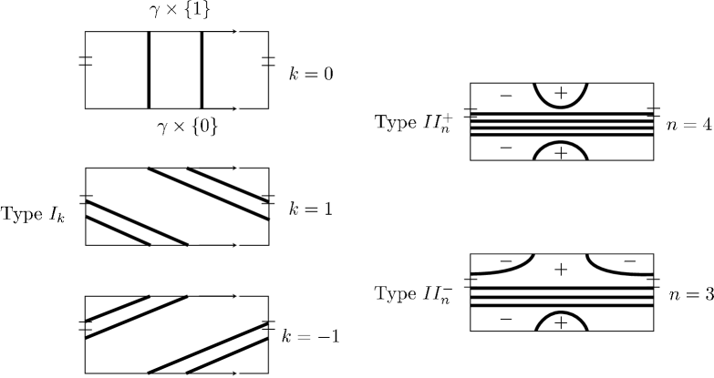
Figure 6. Dividing curves of type ${\mbox{\it I}}_{k}$ and $\mbox{\it II}_{n}^{\pm}$.

4.1. Type $\mbox{\it II}_{n}^{\pm}$, $n$ even.

The first case we treat is $\Gamma_{A}=\mbox{\it II}_{n}^{\pm}$, where $n$ is even.

Lemma 4.4.

$\mbox{\it II}_{2m}^{\pm}$, $m\in\mathbb{Z}^{+}$, can be reduced to $\mbox{\it II}_{0}^{\pm}$.

Proof.

The proof strategy is to start with the convex annulus $A$ with dividing set $\Gamma_{A}$ and then search for a bypass $B$ attached along $A$ such that isotoping $A$ across $B$ will produce a convex annulus $A^{\prime}$ with $\Gamma_{A}^{\prime}$ of decreased complexity. It is important to keep in mind that Theorem 4.1 is false for tori; thus in searching for $B$ we must exploit the assumption that the genus of $\Sigma$ is $\geq 2$.

Assume we have $\mbox{\it II}_{2m}^{+}$. Figure 7 depicts the convex decomposition sequence for this case. We will treat the case $m=1$, which is the hardest case. The situation $m>1$ will be left to the reader.

Figure 7(A) depicts $M$ cut open along $A$. Figure 7(A) shows $(\Sigma\setminus\gamma)\times\{1\}$ together with $A^{+}$ and $A^{-}$, two copies of $A$ on $M\setminus A$. (Warning: $A^{+}$ and $A_{+}$ are distinct surfaces. $A_{+}\subset A$ is reserved for the positive region of a convex annulus $A$, whereas $A^{+}$ is the copy of $A$ in $M\setminus A$ where the induced orientation from $A$ agrees with the the orientation induced from $\partial(M\setminus A)$.) Figure 7(B) depicts $(\Sigma\setminus\gamma)\times\{0\}$.

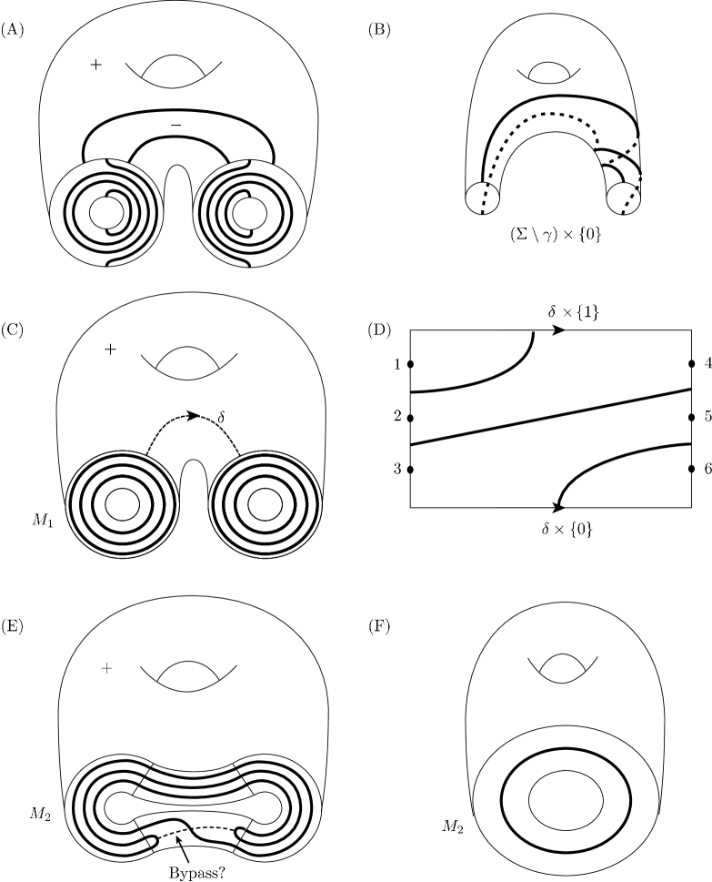
Figure 7. The case $\mbox{\it II}_{2m}^{+}$.

After rounding the edges of $M\setminus A$, we obtain the convex handlebody $M_{1}$ in Figure 7(C). The dividing set $\Gamma_{\partial M_{1}}$ then consists of three parallel curves isotopic to the core curve of $A^{+}$ and three parallel curves isotopic to the core of $A^{-}$.

We now make the next cut in the convex decomposition along $\delta\times I$, where $\delta\subset\Sigma\setminus\gamma$ is a properly embedded oriented arc which connects the two boundary components of $\Sigma\setminus\gamma$ (from $A^{+}$ to $A^{-}$). (Some rounding will have taken place, but we assume that has already been taken care of.) $\delta\times I$ will be given the orientation induced from $\delta$ and $I$. We now consider the dividing curve configurations on $\delta\times I$. $\partial(\delta\times I)$ will intersect $\Gamma_{\partial M_{1}}$ in three points along $A^{+}$ and in three points along $A^{-}$. We label them 1, 2, 3 on $A^{+}$ in order from closest to $\delta\times\{1\}$ to farthest from $\delta\times\{1\}$. Similarly label the three points of intersection on $A^{-}$ by 4, 5, 6 from closest to $\delta\times\{1\}$ to farthest (see Figure 7(D)). We claim that if there exists a $\partial$-parallel dividing curve straddling one of Positions 2, 3, 4, or 5, then the bypass corresponding to any of these positions, when considered back on $A$, would give a bypass along $A$ (from one of the sides) and a new convex annulus isotopic to $A$ with fewer dividing curves. Positions 2 and 5 give rise to bypasses whose Legendrian arcs of attachment are contained in $A$ and which intersect three distinct curves of $\Gamma_{A}$. A bypass at Positions 3 or 4, when traced back to Figure 7(A), also yields a bypass along $A$ which reduces $\#\Gamma_{A}$. To realize this, we apply Bypass Sliding (Lemma 1.3). Now, Figure 7(D) is the only remaining dividing curve configuration for $\delta\times I$.

Therefore, we can either reduce from $\mbox{\it II}_{2}^{+}$ to $\mbox{\it II}_{0}^{+}$ or obtain the dividing set as in Figure 7(D). In the latter situation, we proceed by rounding the edges of $M_{1}\setminus(\delta\times I)$ to get $M_{2}$, depicted in Figure 7(E). This, after the unique dividing curve is straightened, is equivalent to Figure 7(F). In other words, $\Gamma_{\partial M_{2}}$ consists of one curve, and it separates $\partial M_{2}$.

We claim there exists a bypass from the interior of $\partial M_{2}$ along $(\delta\times I)^{-}$ as depicted in Figure 7(E). This follows from using Lemma 1.4 with $F=\partial M_{2}$. Once we have the bypass, adding it to the exterior of $(\delta\times I)^{+}$ as shown in Figure 7(E) forces the existence of bypasses in Positions 3 and 4. Therefore, we can always reduce from $\mbox{\it II}^{\pm}_{2m}$ to $\mbox{\it II}^{\pm}_{0}$. ∎

Lemma 4.5.

$\Gamma_{A}=\mbox{\it II}_{0}^{\pm}$ extends uniquely to a tight contact structure on $M$. It is universally tight.

Proof.

After cutting $M$ along $A$, we obtain $M\setminus A=S\times I$, where $S$ is a surface of genus $g-1$ with two punctures. Applying edge-rounding, we obtain that $\Gamma_{\partial(S\times I)}$ is isotopic to $(\partial S)\times\{{1\over 2}\}$. Lemma 4.2 (or the proof of Lemma 4.2) implies that there is a unique tight contact structure which extends to the interior of $S\times I$. The tight contact structure is universally tight by Lemma 4.2, and glues to give a universally tight contact structure on $M$, since $\Gamma_{A}$ is $\partial$-parallel and we can therefore apply Theorem 4.3. ∎

4.2. Type $\mbox{\it II}_{n}^{\pm}$, $n$ odd.

Lemma 4.6.

$\mbox{\it II}_{2m+1}^{\pm}$, $m\in\mathbb{Z}^{+}$, can be reduced to $\mbox{\it II}^{\pm}_{1}$.

Proof.

The proof is similar to the proof of Lemma 4.4. It is enough to show that $\mbox{\it II}_{2m+1}^{\pm}$ can be reduced to $\mbox{\it II}_{2m-1}^{\pm}$. Figure 8(A) depicts $M\setminus A$ where we have $\mbox{\it II}_{2m+1}^{+}$. After rounding the edges, we obtain $M_{1}$ which has $2m+3$ closed curves parallel to the core curve of $A^{+}$ and $2m+1$ closed curves parallel to the core curve of $A^{-}$. We take the next convex decomposing disk $\delta\times I$ with efficient Legendrian boundary. $\partial(\delta\times I)$ intersects $\Gamma_{\partial M_{1}}$ in $2m+3$ points along $A^{+}$, labeled $1$ through $2m+3$ from closest to $\delta\times\{1\}$ to farthest from $\delta\times\{1\}$, and $2m+1$ points along $A^{-}$, labeled $2m+4$ through $4m+4$. The only $\partial$-parallel dividing curves on $\delta\times I$ which do not immediately lead to a bypass on $A$ are those straddling Positions $1$ and $2m+3$. Therefore, we are left to consider a unique choice for $\Gamma_{\delta\times I}$, given in Figure 8(C), i.e., exactly two $\partial$-parallel arcs (along $1$ and $2m+3$), and all other dividing curves consecutively nested around them.

In order to prove the reduction from $\mbox{\it II}_{2m+1}^{\pm}$ to $\mbox{\it II}^{\pm}_{2m-1}$, we show the existence of a nontrivial bypass along $(\delta\times I)^{-}$ from the interior of $M_{2}$. Indeed, Lemma 1.4 guarantees that there is a bypass along an arc of attachment which intersects the $\partial$-parallel component of $(\delta\times I)^{-}$ straddling Position $1$, as well as two consecutively nested dividing arcs. See Figure 8(D). This bypass, if viewed on $\delta\times I$ (Figure 8(C)), produces $\partial$-parallel curves across Positions $2m+2$ and $4m+3$, giving us a reduction in the number of parallel curves on $\Gamma_{A}$. ∎

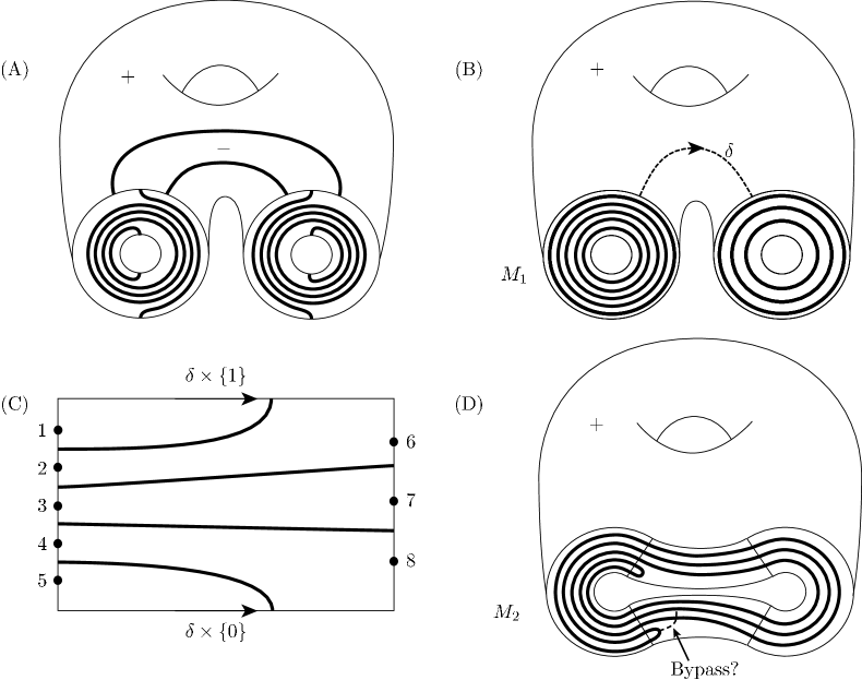
Figure 8. The case $\mbox{\it II}_{2m+1}^{+}$.

Lemma 4.7.

$\mbox{\it II}^{\pm}_{1}$ can be reduced to ${\mbox{\it I}}_{k}$.

Proof.

We will treat $\Gamma_{A}=\mbox{\it II}^{-}_{1}$, and leave $\mbox{\it II}^{+}_{1}$ to the reader. The computation is similar in spirit to the previous computations, except that it is a bit more involved. The goal is to find a bypass along $A^{+}$ from the interior of $M_{1}$ which straddles the three components of $\Gamma_{A^{+}}$. This time, the holonomy of the bypass (how many times the bypass wraps around the core curve) is important. In order to determine the existence of a bypass, we will successively cut $M_{1}$, leaving $A^{+}$ untouched, until we arrive at a solid torus whose boundary contains $A^{+}$. On the solid torus, we can determine whether the bypass exists, by appealing to the classification of tight contact structures on solid tori [11, 14].

Figure 9. The case $\mbox{\it II}_{1}^{-}$.

Figures 9 and 10 depict this decomposition process. As shown in Figure 9(B), let $\delta_{1}$ be a non-boundary-parallel, properly embedded arc on $\Sigma\setminus\gamma$ which does not intersect $\delta$ and begins and ends on $\partial A^{-}$. We take $\partial(\delta_{1}\times I)$ to be Legendrian and efficient with respect to $\Gamma_{\partial M_{1}\setminus A^{+}}$ on $\partial M_{1}\setminus A^{+}$. Note this happens to be the same as being efficient with respect to $\Gamma_{\partial M_{1}}$ on $\partial M_{1}$. The side of Figure 9(A) which is hidden, namely $(\Sigma\setminus\gamma)\times\{0\}$, is as shown in Figure 7(B), that is, the hidden side differs from the top by a single Dehn twist. However, for subsequent figures, we suppose that the $\partial$-parallel dividing curve on $A^{-}$ along $(\gamma\times\{0\})^{-}$ has already been twisted around the core curve of $A^{-}$, i.e., $\Gamma_{(\Sigma\setminus\gamma)\times\{0\}}$ is the same as $\Gamma_{(\Sigma\setminus\gamma)\times\{1\}}$. Now, take $\delta_{1}\times I$ to be convex and define $M_{2}$ to be $M_{1}\setminus(\delta_{1}\times I)$, after rounding the edges. (Warning: This $M_{2}$ is different from the $M_{2}$’s in the previous lemmas.) We label $\partial(\delta_{1}\times I)\cap\Gamma_{\partial M_{1}}$ by numbers $1$ through $6$ as follows: There is a unique closed curve of $\Gamma_{\partial M_{1}\setminus A^{+}}$, and we let the two points of intersection of this curve with $\partial(\delta_{1}\times I)$ be $2$ and $5$. The rest are labeled in increasing order along $\partial(\delta_{1}\times I)$ in the direction given by the induced orientation, i.e., “counterclockwise”. Now, $\partial$-parallel dividing curves in Positions $2$ and $5$ would immediately allow us to reduce to $I_{k}$, as can be seen on the $(\delta_{1}\times I)^{-}$-side. Therefore, we are left with two possibilities for $\Gamma_{\delta_{1}\times I}$, which we call $\beta_{1}$ and $\beta_{2}$. In Figure 9(D), the left diagram represents the two $\partial$-parallel positions which are ruled out, and the middle and right respectively are $\beta_{1}$ and $\beta_{2}$.

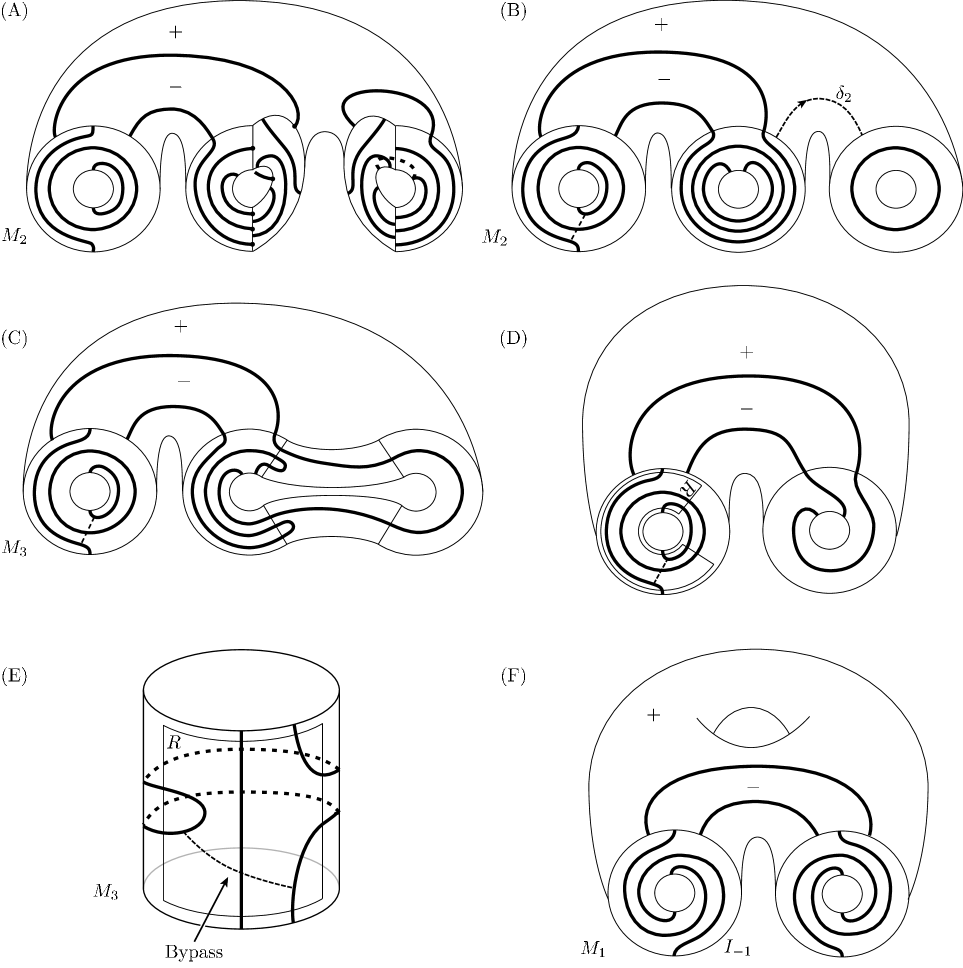
Figure 10. The case $\mbox{\it II}_{1}^{-}$, continued. Configuration $\beta_{1}$.

Consider $\beta_{1}$. (See Figure 10.) Figure 10(A) represents the dividing set $\Gamma_{\partial M_{2}}$ before rounding, and Figure 10(B) is $\Gamma_{\partial M_{2}}$ after rounding. We take $\delta_{2}$ (as in Figure  10(B)) to be a non-boundary-parallel, properly embedded arc on $\Sigma\setminus(\gamma\cup\delta_{1})$ which begins on one copy of $\delta_{1}$ and ends on the other copy. At this point, $\Sigma\setminus(\gamma\cup\delta_{1})$ is a pair-of-pants, and cutting along $\delta_{2}$ yields an annulus. Take $\partial(\delta_{2}\times I)$ to be Legendrian and efficient with respect to $\Gamma_{\partial M_{2}\setminus A^{+}}$ (which also happens to be the same as being efficient with respect to $\Gamma_{\partial M_{2}}$). Now, $tb(\partial(\delta_{2}\times I))=-2$, and there are two possibilities for $\Gamma_{\delta_{2}\times I}$. We may rule out one of the possibilities, since it yields a $\partial$-parallel dividing curve which allows us to reduce to $I_{k}$.

Finally, we have a solid torus $M_{3}=M_{2}\setminus(\delta_{2}\times I)$, and $\Gamma_{\partial M_{3}}$ consists of 2 parallel longitudinal dividing curves. (Figures 10(C,D,E) represent $\Gamma_{\partial M_{3}}$ before and after successive edge-roundings.) A compressing disk $D$ intersecting each dividing curve once may be chosen so that $M_{3}\setminus D$ is as shown in Figure 10(E), and in particular so that the rectangles labelled $R$ in Figure 10(D) and Figure 10(E) correspond. This implies, by [14], that $M_{3}$ is a standard neighborhood of a Legendrian curve. Let us identify $\partial M_{3}=\mathbb{R}^{2}/\mathbb{Z}^{2}$ by letting the meridian have slope $0$ and $\Gamma_{\partial M_{3}}$ have slope $\infty$.

We claim that there exists a bypass along $A^{+}$ from the interior of $M_{1}$, which changes $\mbox{\it II}^{-}_{1}$ to ${\mbox{\it I}}_{-1}$. We look for the corresponding bypass along $A^{+}$ on $M_{3}$. To see this exists, let $D$ be a convex meridional disk for $M_{3}$ with Legendrian boundary $\partial D$ which is efficient with respect to $\Gamma_{\partial M_{3}}$ and is disjoint from the bypass arc of attachment. Then $tb(\partial D)=-1$, and there is a unique way, up to isotopy, to cut this solid torus into a 3-ball $B^{3}$. Finally, the bypass along $\partial B^{3}$ is a trivial bypass, which must therefore exist by Right-to-Life. ∎

4.3. Type ${\mbox{\it I}}_{k}$.

Lemma 4.8.

${\mbox{\it I}}_{k}$, $k>0$, can be reduced to ${\mbox{\it I}}_{0}$.

Proof.

The decomposition procedure is given in Figure 11. Figure 11(A) gives $M\setminus A$; note that in this figure $\Gamma_{(\Sigma\setminus\gamma)\times\{0\}}$ does not equal $\Gamma_{(\Sigma\setminus\gamma)\times\{1\}}$ and rather is as in Figure 7(B). Figure 11(B) is the same as Figure 11(A), except that the extra Dehn twist is incorporated in $A^{-}$ so that $\Gamma_{(\Sigma\setminus\gamma)\times\{0\}}=\Gamma_{(\Sigma\setminus\gamma)\times\{1\}}$. Figure 11(C) depicts $\partial M_{1}$, where $M_{1}$ is $M\setminus A$ with the edges rounded.

Figure 11. The case ${\mbox{\it I}}_{k}$, $k>0$.

Let $\delta\subset\Sigma\setminus\gamma$ be the same as in Lemma  4.4. As before, consider the compressing disk $\delta\times I$, which we take to be convex with efficient Legendrian boundary. $\delta\times I$ is chosen so that $\partial(\delta\times I)$ intersects $\Gamma_{\partial M_{1}}$ in $2k-1$ points along $A^{+}$ (labeled $1$ through $2k-1$ in order from closest to $\delta\times\{1\}$ to farthest) and $2k+3$ points along $A^{-}$ (labeled $2k$ through $4k+2$ in order from closest to $\delta\times\{1\}$ to farthest). If there are $\partial$-parallel components of $\Gamma_{\delta\times I}$ along any of $2k+1,\dots,4k+1$, then the corresponding bypasses would give rise to the state transition from ${\mbox{\it I}}_{k}$ to ${\mbox{\it I}}_{k-1}$. Now, there are $2k+2$ endpoints of $\Gamma_{\delta\times I}\cap\partial(\delta\times I)$ between Positions $2k$ and $4k+2$. If there are connections (dividing arcs) amongst the $2k+2$ endpoints, then clearly, this would give rise to a $\partial$-parallel arc straddling one of the “reducing” positions. However, this must happen since the total number of endpoints is $4k+2$, i.e., $\#(\Gamma_{\delta\times I}\cap\partial(\delta\times I))=4k+2$, and $4k+2<2(2k+2)$. ∎

Lemma 4.9.

${\mbox{\it I}}_{k}$, $k<-1$, can be reduced to ${\mbox{\it I}}_{-1}$.

The apparent lack of symmetry between Lemmas 4.8 and 4.9 is due to the fact that the first cut along $A$ is not symmetric with respect to $\Gamma_{0}$.

Proof.

The argument is almost identical to that of Lemma 4.8. The only difference is that the computations are mirror images of those of Lemma  4.8. Refer to Figure 12 for the steps of the computation. ∎

Figure 12. The case ${\mbox{\it I}}_{k}$, $k<-1$.

Lemmas 4.8 and 4.9 together indicate that all the ${\mbox{\it I}}_{k}$’s can be reduced to either ${\mbox{\it I}}_{0}$ or ${\mbox{\it I}}_{-1}$. The following Lemma  computes (an upper bound for) the tight contact structures where $\Gamma_{A}={\mbox{\it I}}_{0}$, and relates them to ${\mbox{\it I}}_{-1}$.

Lemma 4.10.

There are at most two tight contact structures on $\Sigma\times I$ in the Base Case for which $\Gamma_{A}={\mbox{\it I}}_{0}$. The same also holds for $\Gamma_{A}={\mbox{\it I}}_{-1}$. There exist state transitions along $A$ which allow us to switch between ${\mbox{\it I}}_{0}$ and ${\mbox{\it I}}_{-1}$.

Proof.

Let us take the case $\Gamma_{A}={\mbox{\it I}}_{0}$. Figure 13(A) gives the dividing set of $M\setminus A$, before edge-rounding but after the extra Dehn twist from the bottom face $(\Sigma\setminus\gamma)\times\{0\}$ is included. (Therefore, $\Gamma_{(\Sigma\setminus\gamma)\times\{0\}}=\Gamma_{(\Sigma\setminus\gamma)\times\{1\}}$.) Figure 13(B) is the same after edge-rounding. Now, if we cut along $\delta\times I$, defined as in Lemma 4.8, there are two possibilities for $\Gamma_{\delta\times I}$, since $tb(\partial(\delta\times I))=-2$. (These are shown in Figures 13(C,D).) Figures 13(E,F) depict the dividing set of $M_{2}=M_{1}\setminus(\delta\times I)$, after edge-rounding. In both cases, $\Gamma_{\partial M_{2}}$ consists of exactly one dividing curve parallel to $\partial(\Sigma\setminus(\gamma\cup\delta))$. Finally, using Lemma  4.2, we find that for each of the two possibilities of $\Gamma_{\delta\times I}$ there is a unique universally tight contact structure on $M_{2}$. Theorem 4.3 is also sufficient to glue back along $\delta\times I$ to give two universally tight contact structures on $M_{1}$ with the boundary condition given by Figure 13(A). Making the final gluing and proving the resulting contact structure is universally tight is a more complicated state-transition operation, so we will content ourselves for the time being with the knowledge that there are at most two tight contact structures on $\Sigma\times I$ in the Base Case with $\Gamma_{A}={\mbox{\it I}}_{0}$. A similar computation also holds for $\Gamma_{A}={\mbox{\it I}}_{-1}$.

Figure 13. Classification for ${\mbox{\it I}}_{0}$.

We now prove that we may switch from ${\mbox{\it I}}_{0}$ to ${\mbox{\it I}}_{-1}$. The reverse procedure is identical. Above, we found that $\#(\Gamma_{\partial M_{1}}\cap\partial(\delta\times I))=4$, and one intersection was on $A^{+}$ (labeled $1$) and $3$ on $A^{-}$ (labeled $2,3,4$ in succession from closest to $\delta\times\{1\}$ to farthest). A $\partial$-parallel dividing curve of $\delta\times I$ straddling Position $3$ clearly allows us to transition from ${\mbox{\it I}}_{0}$ to ${\mbox{\it I}}_{-1}$. On the other hand, a $\partial$-parallel dividing curve straddling Position $4$ gives rise to a corresponding bypass which can be slid so that all three of the intersections with $\Gamma_{\partial M_{1}}$ lie on $A^{-}$. Therefore, for both choices of $\Gamma_{\delta\times I}$, we may transition from ${\mbox{\it I}}_{0}$ to ${\mbox{\it I}}_{-1}$. ∎

4.4. Completion of Theorem 4.1.

Summarizing what we have proved so far:

• $\#\pi_{0}(Tight(M,\mathcal{F}))\leq 4.$

• Type $\mbox{\it II}^{+}_{0}$: there exists one.

• Type $\mbox{\it II}^{-}_{0}$: there exists one.

• Type ${\mbox{\it I}}_{0}$: there are at most $2$.

• The other possibilities for $\Gamma_{A}$ reduce to one of $\mbox{\it II}^{\pm}_{0}$ or ${\mbox{\it I}}_{0}$.

• The tight contact structures of type $\mbox{\it II}^{\pm}_{0}$ are universally tight by Lemma 4.5.

• The tight contact structures of type $\mbox{\it II}^{+}_{0}$ and $\mbox{\it II}^{-}_{0}$ are distinct and are also distinct from those of type ${\mbox{\it I}}_{0}$ by the relative Euler class $\tilde{e}$ evaluated on $A$.

The proof of Theorem 4.1 is complete, once we show Lemmas 4.11 and 4.13 below.

Lemma 4.11.

There are exactly two tight contact structures of type ${\mbox{\it I}}_{0}$. They are universally tight, are obtained by adding a single bypass onto $\Sigma_{0}$, and have relative Euler class $PD(\tilde{e}(\xi))=\pm(\gamma_{1}-\gamma_{0})$.

Proof.

We show the existence of the (universally) tight contact structures by embedding them inside a suitable (universally) tight contact structure of type $\mbox{\it II}^{\pm}_{0}$. Let $A=\gamma\times I$ be the first cut that was used to decompose $\Sigma\times I$. If $\Gamma_{A}=\mbox{\it II}^{+}_{0}$, then there is a $\partial$-parallel dividing curve along $\gamma\times\{0\}$ which cuts off a positive region of $A$. There is a corresponding degenerate bypass whose Legendrian arc of attachment is all of $\gamma\times\{0\}$. (Degenerate means that the two ends of the Legendrian arc of attachment are identical.) If we immediately attach this degenerate bypass onto $\Sigma_{0}$, we obtain an isotopic convex surface which we call $\Sigma_{1/2}^{\prime}$ and which satisfies $\Gamma_{\Sigma_{1/2}^{\prime}}=2\gamma$. However, if we separate the endpoints by bypass sliding in one particular direction along $\Gamma_{\Sigma_{0}}$, we obtain a more convenient convex surface $\Sigma_{1/2}$ with $\Gamma_{\Sigma_{1/2}}=2\gamma_{1}$, after the bypass attachment. There are two possible bypasses (of opposite sign) we can attach to $\Sigma_{0}$, arising from $\mbox{\it II}^{+}_{0}$ and $\mbox{\it II}^{-}_{0}$. They are clearly universally tight by construction.

We now compute their relative Euler class. It will then be clear that the two tight contact structures are distinct and of type ${\mbox{\it I}}_{0}$. We fix some notation. The tight contact structure $\xi$ obtained in the previous paragraph by attaching a bypass has ambient manifold $\Sigma\times[0,1]$, $\Gamma_{\Sigma_{i}}=2\gamma_{i}$, $i=0,1$, and $\xi$ is $[0,1]$-invariant except for $\mathcal{A}\times[0,1]$, where $\mathcal{A}\subset\Sigma_{0}$ is a convex annulus with Legendrian boundary whose core curve is isotopic to $\gamma$, and the bypass was attached to $\Sigma_{0}$ along $\mathcal{A}$.

First suppose $\beta\subset\Sigma$ is a closed nonseparating curve which intersects neither $\gamma_{0}$ nor $\gamma_{1}$. Then the corresponding convex annulus $\beta\times I$ will only consist of closed curves parallel to the core curve. Hence $\langle\tilde{e}(\xi),\beta\times I\rangle=0$. Thus we may choose a basis of $H_{1}(\Sigma;\mathbb{Z})$ such that, of the $2g$ generators, $2g-2$ of them evaluate to zero in this manner. Next let $\beta\times\{0\}\subset\Sigma_{0}$ be a closed Legendrian curve parallel to $\gamma$ but disjoint from $\mathcal{A}$. Then, since $\xi$ is $I$-invariant away from $\mathcal{A}\times I$, $\beta\times I$ must consist of $2$ parallel vertical nonseparating arcs, that is, $\langle\tilde{e}(\xi),\beta\times I\rangle=0$. Finally, let $\beta\times\{0\}\subset\Sigma_{0}$ be a closed efficient Legendrian curve which is parallel to $\gamma_{1}$ but does not intersect the arc of attachment of the bypass, which we take to be nondegenerate. Then $\beta\times\{i\}$, $i=0,1$, intersects $\Gamma_{\Sigma_{i}}$ twice, and $\Gamma_{\beta\times I}$ consists of 2 parallel vertical nonseparating arcs. However, now $\beta\times\{1\}$ is not efficient with respect to $\Gamma_{\Sigma_{i}}$, and resolving the extra intersection to produce an efficient intersection gives $\langle\tilde{e}(\xi),(\beta\times I)^{*}\rangle=\pm 1$. (Here, $(\cdot)^{*}$ refers to the annulus with efficient Legendrian boundary.) See Figure 14. Having evaluated $\tilde{e}(\xi)$ on all the basis elements, we find that $PD(\tilde{e}(\xi))=\pm\gamma=\pm(\gamma_{1}-\gamma_{0})$. ∎

Figure 14. Ocarinian Riemann surfaces

Definition 4.12.

A tight contact structure on $\Sigma\times I$ which is contact diffeomorphic to one of the tight contact structures of type ${\mbox{\it I}}_{0}$ is said to be a basic slice. Thus, in a basic slice, $\Gamma_{\Sigma\times\{0\}}$ and $\Gamma_{\Sigma\times\{1\}}$ each consist of two parallel curves $2\gamma_{0}$ and $2\gamma_{1}$ with $|\gamma_{0}\cap\gamma_{1}|=1$. The basic slice is obtained by attaching a single bypass $B$ onto $\Sigma\times\{0\}$ and thickening $(\Sigma\times\{0\})\cup B$.

Lemma 4.13.

The tight contact structure of type $\mbox{\it II}^{\pm}_{0}$ has relative Euler class $PD(\tilde{e}(\xi))=\mp(\gamma_{1}+\gamma_{0})$.

Proof.

We will restrict our attention to $\mbox{\it II}^{+}_{0}$. As in the proof of Lemma 4.11, if $\beta\subset\Sigma$ is a closed nonseparating curve which does not intersect $\gamma_{0}$ or $\gamma_{1}$, then $\langle\tilde{e}(\xi),\beta\times I\rangle=0$. From the definition of $\mbox{\it II}^{+}_{0}$ we have:

$$\langle\tilde{e}(\xi),(\gamma_{1}-\gamma_{0})\times I\rangle=2.$$

Next, since $\gamma_{0}\times I$ with efficient Legendrian boundary intersects $\Gamma_{\Sigma_{0}}$ $0$ times and $\Gamma_{\Sigma_{1}}$ twice,

$$\langle\tilde{e}(\xi),\gamma_{0}\times I\rangle=\pm 1,$$

where the exact sign will be determined in a moment. Similarly,

$$\langle\tilde{e}(\xi),\gamma_{1}\times I\rangle=\pm 1.$$

For the three equations to agree, we must have $\langle\tilde{e}(\xi),\gamma_{0}\times I\rangle=-1$ and $\langle\tilde{e}(\xi),\gamma_{1}\times I\rangle=1$. This implies that $PD(\tilde{e}(\xi))=-(\gamma_{1}+\gamma_{0})$. ∎

5. Classification of tight contact structures on $\Sigma\times I$

In this section we prove Theorem 0.1 as well as the following theorem:

Theorem 5.1 (Gluing Theorem).

Let $\Sigma$ be an oriented closed surface of genus $g\geq 2$, $M=\Sigma\times[0,2]$, and $\xi$ a contact structure which is tight on $M\setminus\Sigma_{1}$. Suppose $\Sigma_{i}$, $i=0,1,2$, are convex and $\Gamma_{\Sigma_{i}}=2\gamma_{i}$, where $\gamma_{i}$ are nonseparating oriented curves. Also assume that the $\gamma_{i}$ are not mutually homologous. If $PD(\tilde{e}(\xi|_{\Sigma\times[0,1]}))=\gamma_{1}-\gamma_{0}$ (here $\gamma_{0}$ and $\gamma_{1}$ have been oriented so the relative Euler class has this form), then $PD(\tilde{e}(\xi|_{\Sigma\times[1,2]}))=\gamma_{2}-\gamma_{1}$ (for some orientation of $\gamma_{2}$) if and only if $\xi$ is tight on $M$.

The condition of the $\gamma_{i}$ being mutually nonhomologous is a technical condition, which can be removed if we reformlate the Gluing Theorem without reference to the relative Euler class. The reader is encouraged to do so, after examining the proof of Theorem 0.1 and the Gluing Theorem. As we will see, the only contact topology calculations needed to prove Theorem 0.1 are the one done in Section 4 and a similar calculation in Proposition 5.3. The rest is largely a “proof by pure thought”, relying on the relative Euler class consistency check, Proposition 5.2, and curve complex facts.

5.1. Freedom of choice

The proof of Theorem 0.1 is founded on the following rather remarkable proposition.

Proposition 5.2 (Freedom of choice).

Let $(M=\Sigma\times I,\xi)$ be a basic slice with $\Gamma_{\Sigma_{i}}=2\gamma_{i}$, $i=0,1$ and $\langle\gamma_{1},\gamma_{0}\rangle=+1$, where $\langle\cdot\rangle$ represents the intersection form on $\Sigma$, a surface of genus at least $2$. Let $\gamma$ be any nonseparating curve on $\Sigma$. Then there exists a convex surface isotopic to $\Sigma_{0}$ (or, equivalently, to $\Sigma_{1}$), which we call $\Sigma_{1/2}$ and which has $\Gamma_{\Sigma_{1/2}}=2\gamma$.

The strategy of the proof is to start with $\Gamma_{\Sigma_{0}}=2\gamma_{0}$ and $\Gamma_{\Sigma_{1}}=2\gamma_{1}$ and successively find subslices $\Sigma\times[a,b]\subset\Sigma\times[0,1]$ with convex boundary and dividing sets $\Gamma_{\Sigma_{a}}$, $\Gamma_{\Sigma_{b}}$ which consist of two parallel curves each and represent curves which are “closer” to $\gamma$ inside the curve complex. To prevent our notation from becoming to cumbersome, we will rename the old $\Sigma\times[a,b]$ to be the new $\Sigma\times[0,1]$ after each step of the induction. We also write $[\alpha_{0},\alpha_{1};PD(\tilde{e}(\xi))]$ to mean some tight contact structure on $\Sigma\times[0,1]$ with $\Gamma_{\Sigma_{i}}=2\alpha_{i}$, $i=0,1$ and relative Euler class $PD(\tilde{e}(\xi))$. If we do not specify the relative Euler class (or it is understood), we simply write $[\alpha_{0},\alpha_{1}]$. Moreover, if we want to indicate a basic slice, we write $\llbracket\alpha_{0},\alpha_{1}\rrbracket$.

We first describe the operation which will be used repeatedly in the proof.

Operation.

Consider $[\alpha_{0},\alpha_{1}]$, where $|\alpha_{0}\cap\alpha_{1}|=1$. Let $\alpha$ be a closed (necessarily nonseparating) curve which satisfies $|\alpha_{0}\cap\alpha|=0$ and $|\alpha_{1}\cap\alpha|=1$. Then there exists a convex surface $\Sigma_{1/2}$ with $\Gamma_{\Sigma_{1/2}}=2\alpha$.

Proof of Operation..

On $\Sigma_{0}$, use LeRP to realize $\alpha\times\{0\}$ as a Legendrian curve with $\#(\Gamma_{\Sigma_{0}}\cap\alpha)=0$. Similarly, Legendrian realize $\alpha\times\{1\}$ with $\#(\Gamma_{\Sigma_{1}}\cap\alpha)=2$. Take the convex annulus $\alpha\times I$. By the Imbalance Principle of [14], there must be a $\partial$-parallel dividing curve along $\alpha\times\{1\}$ and hence a degenerate bypass. Attaching the degenerate bypass gives an isotopic convex surface with $\Gamma=2\alpha$. ∎

Proof of Proposition 5.2..

We start with $\llbracket\gamma_{0},\gamma_{1}\rrbracket$. Using Proposition 2.5, we obtain a sequence:

$$\gamma_{0}=\alpha_{0},\gamma_{1}=\alpha_{1},\alpha_{2},\dots,\gamma=\alpha_{k},$$

where $\alpha_{i}$, $i=0,\dots,k$, are nonseparating, $|\alpha_{i-1}\cap\alpha_{i}|=1$, $i=1,\dots,k$, and $|\alpha_{i-1}\cap\alpha_{i+1}|=0$, $i=1,\dots,k-1$. (Note that the statement of the proposition does not quite give what we want, but the proof clearly does.) Now, using the Operation, we successively find:

$$\llbracket\alpha_{0},\alpha_{1}\rrbracket\supset\llbracket\alpha_{2},\alpha_{1}\rrbracket\supset\llbracket\alpha_{2},\alpha_{3}\rrbracket\supset\dots\supset\llbracket\alpha_{k-1},\alpha_{k}\rrbracket.$$

This completes the proof of the proposition. ∎

5.2. Proof of Part 3 of Theorem 0.1.

We will now give the classification result for $[\gamma_{0},\gamma_{1}=\gamma_{0}]$, where $\gamma_{0}$ is an oriented nonseparating curve. If the tight contact structure $\xi$ is $I$-invariant, then $PD(\tilde{e}(\xi))=0$.

Proposition 5.3.

Let $[\gamma_{0},\gamma_{0}]$ be a tight contact structure on $M=\Sigma\times[0,1]$ which is not $I$-invariant. Then $\Sigma\times[0,1]$ contains some basic slice $\Sigma\times[a,b]$.

Proof.

The proof is a calculation along the lines of Section 4. Let $\gamma\subset\Sigma$ be an oriented curve so that $\langle\gamma,\gamma_{0}\rangle=+1$. Let $A=\gamma\times I$ be a convex annulus with efficient Legendrian boundary. $\Gamma_{A}$ has the possibilities as in Figure 6, denoted types ${\mbox{\it I}}_{k}$ and $\mbox{\it II}^{\pm}_{n}$. Types $\mbox{\it II}^{\pm}_{n}$ all have $\partial$-parallel dividing curves, which give rise to bypasses which, in turn, yield basic slices. Therefore, it suffices to consider ${\mbox{\it I}}_{k}$.

If $\Gamma_{A}={\mbox{\it I}}_{0}$, then there exists a sequence of convex meridional disks $D_{i}$ which decompose $M_{1}=M\setminus A$ into the 3-ball, and for which $tb(\partial D_{i})=-1$. Hence, there must be a unique tight contact structure with $\Gamma_{A}={\mbox{\it I}}_{0}$. This implies that $\Gamma_{A}={\mbox{\it I}}_{0}$ represents the $I$-invariant case.

Figure 15. Transition from ${\mbox{\it I}}_{k}$ to $\mbox{\it II}^{\pm}_{n}$.

Suppose $\Gamma_{A}={\mbox{\it I}}_{k}$ with $k>0$. Let $M_{1}=M\setminus A$. Figure 15(A) gives $M_{1}$ and Figure 15(B) the same with the edges of $A^{-}$ rounded. (Note that Figure 15 depicts the case $\Gamma_{A}=I_{1}$.) They are presented in almost identical fashion as in Section 4 with one exception: now $\Gamma_{(\Sigma\setminus\gamma)\times\{1\}}=\Gamma_{(\Sigma\setminus\gamma)\times\{0\}}.$ Our notation will be identical to that of Lemma  4.7. Let $\delta_{1}$ be an arc in $\Sigma\setminus\gamma$ with $\partial\delta_{1}=p_{1}-p_{0}$, where $p_{0}\in A^{+}$, $p_{1}\in A^{-}$, and $\delta_{1}$ does not intersect $\Gamma_{\Sigma}$. Take $\delta_{1}\times I$ and perturb it to be convex with Legendrian boundary so that $|\partial(\delta_{1}\times I)\cap\Gamma_{\partial M_{1}}|=4k+2$, and $2k+1$ of the intersections we may assume are on $p_{0}\times I$ (labeled $1,\dots,2k+1$ from closest to $\delta_{1}\times\{1\}$ to farthest) and the other $2k+1$ on $p_{1}\times I$ (labeled $2k+2,\dots,4k+2$ from farthest from $\delta_{1}\times\{1\}$ to closest). If there is a $\partial$-parallel dividing arc on $\delta_{1}\times I$ straddling Positions $2,\dots,2k$ or $2k+3,\dots,4k+1$, then the corresponding bypass state transitions us into ${\mbox{\it I}}_{k-1}$. If we can continue this, we eventually get to ${\mbox{\it I}}_{0}$, which is already taken care of. (Actually, it is unlikely such a state transition exists; we probably have an overtwisted contact structure here.) Otherwise, we have two possibilities: $\beta_{1}$ and $\beta_{2}$.

Figure 16. Transition from ${\mbox{\it I}}_{k}$ to $\mbox{\it II}^{\pm}_{n}$, continued.

The case of $\beta_{1}$ occupies Figures 16(A,B) and the case of $\beta_{2}$ occupies Figure 16(C). We will explain $\beta_{2}$ first. After rounding the edges, $\Gamma_{\partial M_{2}\setminus A^{+}}$ has one $\partial$-parallel arc along each boundary component of $A^{+}$. This implies that there exists a Legendrian divide $\alpha_{1}$ on $\partial M_{2}\setminus A^{+}$ parallel to either boundary component of $A^{+}$ (after possibly perturbing $\partial M_{2}\setminus A^{+}$ as in LeRP). Let $\alpha_{2}$ be an efficient Legendrian curve on $A^{+}$, isotopic to the core curve and satisfying $|\alpha_{2}\cap\Gamma_{A^{+}}|=2$. If we take an annulus spanning $\alpha_{1}$ to $\alpha_{2}$, by the Imbalance Principle we will obtain a degenerate bypass along $\alpha_{2}$. Attaching the degenerate bypass will give the transition to some $\mbox{\it II}^{\pm}_{n}$.

On the other hand, $\beta_{1}$ does not immediately give rise to a $\partial$-parallel arc along $\partial A^{+}$. Therefore, we cut again, this time along $\delta_{2}\times I$, which is convex with efficient Legendrian boundary, to obtain $M_{3}$. Write $\partial\delta_{2}=q_{1}-q_{0}$. Now, $|\partial(\delta_{2}\times I)\cap\Gamma_{\partial M_{2}}|=2k+2$, and $2k+1$ of the intersections are on $q_{0}\times I$, whereas $1$ intersection is on $q_{1}\times I$. If $k>1$, then there will always be a bypass along $q_{0}\times I$, which transitions us to ${\mbox{\it I}}_{k-1}$. On the other hand, there is one extra case when $k=1$ — after the edges are rounded (Figure 16(B)), there exists a $\partial$-parallel arc along $\partial A^{+}$ on $\partial M_{3}\setminus A^{+}$. Therefore, we will always have a state transition to some $\mbox{\it II}^{\pm}_{n}$, provided ${\mbox{\it I}}_{k}$ does not represent an $I$-invariant tight contact structure. ∎

We claim that $PD(\tilde{e}([\gamma_{0},\gamma_{0}]))=\pm 2\gamma_{0}$ or $0$. To see this, first note that if $\beta$ is any curve with $|\gamma_{0}\cap\beta|=0$, then $\langle\tilde{e}([\gamma_{0},\gamma_{0}]),\beta\times I\rangle=0$, since $\Gamma_{\beta\times I}$ consists solely of closed curves parallel to the core curve. This takes care of $2g-1$ generators of $H_{1}(\Sigma;\mathbb{Z})$. Next, if $\beta$ satisfies $|\gamma_{0}\cap\beta|=1$, then $\langle\tilde{e}([\gamma_{0},\gamma_{0}]),\beta\times I\rangle$ is $-2$, $0$, or $2$, depending on the configuration of $\partial$-parallel dividing curves on $\beta\times I$. This proves the claim.

Suppose now that $[\gamma_{0},\gamma_{0}]$ is not $I$-invariant. Let $\gamma\subset\Sigma$ be a closed oriented curve satisfying $\langle\gamma_{0},\gamma\rangle=+1$. By Proposition 5.3, $[\gamma_{0},\gamma_{0}]$ contains a basic slice, and, by the freedom of choice, there exists a factorization into $[\gamma_{0},\gamma]\cup\llbracket\gamma,\gamma_{0};\pm(\gamma_{0}-\gamma)\rrbracket$. (Notation: when we write $[a_{1},a_{2}]\cup[a_{2},a_{3}]\cup\dots\cup[a_{k-1},a_{k}]$, the contact structure is layered in order.) We initially have the possibilities $PD(\tilde{e}([\gamma_{0},\gamma]))=\pm\gamma_{0}\pm\gamma$ from Theorem 4.1. However, by the claim in the previous paragraph, if $PD(\tilde{e}(\llbracket\gamma,\gamma_{0}\rrbracket))=\gamma_{0}-\gamma$, then $PD(\tilde{e}([\gamma_{0},\gamma]))=\pm\gamma_{0}+\gamma$. Therefore, there is a total of 4 possibilities:

$$[\gamma_{0},\gamma_{0}]=[\gamma_{0},\gamma;\pm\gamma_{0}+\gamma]\cup\llbracket\gamma,\gamma_{0};\gamma_{0}-\gamma\rrbracket,$$

or

$$[\gamma_{0},\gamma_{0}]=[\gamma_{0},\gamma;\pm\gamma_{0}-\gamma]\cup\llbracket\gamma,\gamma_{0};-(\gamma_{0}-\gamma)\rrbracket.$$

Lemma 5.4.

All four contact structures are tight, distinct, and can be embedded in a basic slice.

Proof.

Let $\gamma_{0}$, $\gamma_{1}$ be nonseparating curves satisfying $\langle\gamma_{1},\gamma_{0}\rangle=+1$. We claim that $\llbracket\gamma_{0},\gamma_{1};\gamma_{1}-\gamma_{0}\rrbracket$ can be factored into $[\gamma_{0},\gamma_{0}]\cup\llbracket\gamma_{0},\gamma_{1}\rrbracket$, where the first factor is not $I$-invariant. This is a consequence of Proposition 5.2 as follows. First we layer $[\gamma_{0},\gamma_{1}]=[\gamma_{0},\gamma]\cup[\gamma,\gamma_{1}]$, where $|\gamma\cap\gamma_{i}|=1$, $i=0,1$, using Proposition 5.2. Now, applying Proposition 5.2 to $[\gamma,\gamma_{1}]$, we expand:

$$[\gamma_{0},\gamma_{1}]=[\gamma_{0},\gamma]\cup[\gamma,\gamma_{0}]\cup\llbracket\gamma_{0},\gamma_{1}\rrbracket.$$

The union of the first and second slices on the right-hand side of the equality cannot be $I$-invariant by the semi-local Thurston-Bennequin inequality (see [12]). Therefore, we have obtained a factorization

$$\llbracket\gamma_{0},\gamma_{1};\gamma_{1}-\gamma_{0}\rrbracket=[\gamma_{0},\gamma_{0}]\cup\llbracket\gamma_{0},\gamma_{1}\rrbracket.$$

It remains to compute $PD(\tilde{e})$ of the second factor. If we reconcile $PD=\pm 2\gamma_{0}$ or $0$ for the first factor with $PD=\pm(\gamma_{1}-\gamma_{0})$ for the second factor, we easily see that:

$$\llbracket\gamma_{0},\gamma_{1};\gamma_{1}-\gamma_{0}\rrbracket=[\gamma_{0},\gamma_{0};0]\cup\llbracket\gamma_{0},\gamma_{1};\gamma_{1}-\gamma_{0}\rrbracket.$$

We therefore have realized at least one tight contact structure $[\gamma_{0},\gamma_{0};0]$ which is not $I$-invariant. We also obtain another non-$I$-invariant tight contact structure $[\gamma_{0},\gamma_{0};0]$ by starting from $\llbracket\gamma_{0},\gamma_{1};\gamma_{0}-\gamma_{1}\rrbracket$ instead.

Our next claim is that the two non-$I$-invariant $[\gamma_{0},\gamma_{0};0]$ are distinct. Suppose we further factor:

$$\llbracket\gamma_{0},\gamma_{1};\gamma_{1}-\gamma_{0}\rrbracket=[\gamma_{0},\gamma_{1}]\cup\llbracket\gamma_{1},\gamma_{0}\rrbracket\cup\llbracket\gamma_{0},\gamma_{1};\gamma_{1}-\gamma_{0}\rrbracket.$$

The relative Euler classes on the right-hand side of the equation, in order, are $\pm\gamma_{0}\pm\gamma_{1}$, $\pm(\gamma_{0}+\gamma_{1})$, $\gamma_{1}-\gamma_{0}$. (The reason we have $\pm(\gamma_{0}+\gamma_{1})$ for the second term is due to the relative orientations of $\gamma_{0}$ and $\gamma_{1}$.) For the union of the second and third layers to be tight, the second layer must have relative Euler class $\gamma_{0}+\gamma_{1}$ in order to cancel the $\gamma_{0}$’s (and the first layers must be $-(\gamma_{0}+\gamma_{1})$). Therefore,

$$\llbracket\gamma_{0},\gamma_{1};\gamma_{1}-\gamma_{0}\rrbracket=[\gamma_{0},\gamma_{1};-(\gamma_{0}+\gamma_{1})]\cup\llbracket\gamma_{1},\gamma_{0};\gamma_{0}+\gamma_{1}\rrbracket\cup\llbracket\gamma_{0},\gamma_{1};\gamma_{1}-\gamma_{0}\rrbracket.$$

Applying the same calculation to $\llbracket\gamma_{0},\gamma_{1};\gamma_{0}-\gamma_{1}\rrbracket$, we see that the two non-$I$-invariant tight contact structures $[\gamma_{0},\gamma_{0};0]$ can be distinguished by the factorization into $[\gamma_{0},\gamma_{1}]\cup\llbracket\gamma_{1},\gamma_{0}\rrbracket$.

It remains to dig further to obtain the remaining two tight contact structures $[\gamma_{0},\gamma_{0}]$ with $PD(\tilde{e})=\pm\gamma_{0}$. It suffices to factor $\llbracket\gamma_{0},\gamma_{1};\gamma_{1}-\gamma_{0}\rrbracket$ into

$$[\gamma_{0},\gamma_{0};-2\gamma_{0}]\cup\llbracket\gamma_{0},\gamma_{1};\gamma_{0}-\gamma_{1}\rrbracket\cup\llbracket\gamma_{1},\gamma_{0};\gamma_{0}+\gamma_{1}\rrbracket\cup\llbracket\gamma_{0},\gamma_{1};\gamma_{1}-\gamma_{0}\rrbracket.$$

Similarly, we obtain $[\gamma_{0},\gamma_{0};2\gamma_{0}]$. ∎

5.3. Proof of Parts 1 and 2 of Theorem 0.1 and of Theorem 5.1

We first need the following lemma:

Lemma 5.5.

If $\gamma_{0}\not=\gamma_{1}$, then $[\gamma_{0},\gamma_{1}]$ contains a basic slice.

Proof.

First suppose that $|\gamma_{0}\cap\gamma_{1}|\not=0$. Then we can realize $\gamma_{1}\times\{0,1\}$ on $\Sigma_{0}\cup\Sigma_{1}$ by efficient Legendrian curves, apply the Imbalance Principle to the convex annulus with boundary $\gamma_{1}\times\{0,1\}$, and find a bypass along $\gamma_{1}\times\{0\}\subset\Sigma_{0}$ from the interior of $\Sigma\times I$. Let $\alpha$ be the Legendrian arc of attachment for the bypass. There are two possibilities for $\alpha$: (i) $\alpha$ starts on a dividing curve $\gamma_{0}^{1}$ (one of the two curves parallel to $\gamma_{0}$ on $\Sigma_{0}$), passes through the other curve $\gamma_{0}^{2}$, and ends on $\gamma_{0}^{1}$; (ii) $\alpha$ starts on $\gamma_{0}^{1}$, passes through $\gamma_{0}^{2}$, and ends on $\gamma_{0}^{2}$ after going through a nontrivial loop. (i) is clearly an attachment which gives rise to a basic slice. For (ii), let $P\subset\Sigma_{0}$ be a pair-of-pants neighborhood of the union of $\alpha$ and the annulus bounded by $\gamma_{0}^{1}$ and $\gamma_{0}^{2}$. One of the boundary components is a curve $\gamma$ parallel to $\gamma_{0}^{i}$, the second boundary component is $B(\gamma)$, parallel to the dividing curves on $\Sigma_{1/2}$ obtained by isotoping $\Sigma_{0}$ through the bypass attached along $\alpha$ and the third curve denoted $\delta$ may be thought of as the nontrivial loop $\alpha$ goes around (see Figure 19).

We claim that $\gamma=\gamma_{0}$ and $B(\gamma)=\gamma_{1\over 2}$ are not isotopic. If they were, then they would cobound an annulus $B$, and $B\cup P$ would be a once-punctured torus. In a once-punctured torus, an efficient, nontrivial arc or closed curve will intersect another only in positive intersections or only in negative intersections. This contradicts the efficiency of the original curve $\gamma_{1}\times\{0\}$.

Therefore, we may shrink $\Sigma\times[0,1]$ and assume that $\gamma_{0}\not=\gamma_{1}$ are disjoint and nonisotopic. In such a situation, let $\beta$ denote a curve that is efficient, intersects $\gamma_{0}$ and does not intersect $\gamma_{1}$. By using the Imbalance Principle as above, we can again find a bypass of either type (i), in which case we have found a basic slice, or a bypass of type (ii). In the latter case we can shrink again and have $\Sigma\times[0,1]$ with $\Gamma_{\Sigma_{0}}$ parallel to $\gamma$ and $\Gamma_{\Sigma_{1}}$ parallel to $B(\gamma)$, where $\gamma$, $B(\gamma)$ and $\delta$ form a boundary of a pair of pants $P\subset\Sigma_{0}$ and $\gamma$ and $B(\gamma)$ are not isotopic.

Assume $\delta$ is nonseparating. If $\gamma$ and $\delta$ lie on the same connected component of $\Sigma_{0}\setminus int(P)$, let $\beta_{1}$ be an arc in $P$ connecting $\gamma$ and $\delta$ and let $\beta_{2}$ be an arc in $\Sigma_{0}\setminus int(P)$ connecting the same points on $\gamma$ and $\delta$ as $\beta_{1}$. Let $\beta=\beta_{1}\cup\beta_{2}$ (Figure 20, Case $C_{1}$). Since $\beta$ does not intersect $B(\gamma)$, the Imbalance Principle applied to it produces a bypass of type (i), and hence a basic slice.

If $B(\gamma)$ and $\delta$ lie on the same connected component of $\Sigma_{0}\setminus int(P)$, an analogous argument produces $\beta$ that intersects $B(\gamma)$ once and does not intersect $\gamma$, and another application of the Imbalance Principle produces a basic slice. (See Figure 20, Case $C_{2}$.)

If $\delta$ is separating, denote the component of $\Sigma_{0}\setminus P$ it bounds by $S_{1}$. Let $\beta_{1}$ be a nonseparating arc in $S_{1}$ which starts and ends on $\delta$, and let $\beta_{2}$ be a nonseparating arc in another component of $\Sigma_{0}\setminus P$ which starts and ends on $\gamma$. Let $\beta$ be a closed nonseparating curve obtained by joining those arcs by arcs in $P$ (Figure 20, Cases $C_{3}$ and $C_{4}$). Note that a nonseparating $\beta_{2}$ exists and $\beta$ can be chosen efficient and Legendrian in both $\Sigma_{i}$ because $\gamma$ and $B(\gamma)$ are not isotopic. Applying the Imbalance Principle to this $\beta$ produces a bypass of type (ii) with nonseparating $\delta$. This in turn, we have shown, contains a basic slice. ∎

Note. A similar but slightly more involved argument will be carried out in Proposition 6.2. The figures we refer to are the same as the ones we need for that argument.

Now that we know that $[\gamma_{0},\gamma_{1}]$ contains a basic slice, we may apply Proposition 2.5, together with Proposition 5.2, to factor:

$$[\gamma_{0},\gamma_{1}] = \llbracket\alpha_{0}=\gamma_{0},\alpha_{1};\alpha_{1}-\alpha_{0}\rrbracket\cup\llbracket\alpha_{1},\alpha_{2}\rrbracket\cup\dots$$

$$\dots\cup\llbracket\alpha_{k-2},\alpha_{k-1}\rrbracket\cup[\alpha_{k-1},\alpha_{k}=\gamma_{1}],$$

subject to the following:

1. $\alpha_{i}$, $i=1,\dots,k$, are oriented nonseparating curves.

2. $|\alpha_{i}\cap\alpha_{i+1}|=1$ ($i=0,\dots,k-1$) and $|\alpha_{i}\cap\alpha_{i+2}|=0$ ($i=0,\dots,k-2$).

3. $\langle\alpha_{i+1},\alpha_{i}\rangle=1$, $i=0,\dots,k-1$.

4. All the slices except for the last are basic slices.

5. Without loss of generality, $PD(\tilde{e})$ of the first factor is $\alpha_{1}-\alpha_{0}$.

We will inductively prove that the rest of the $PD(\tilde{e})$’s must be, in order, $\alpha_{2}-\alpha_{1},\alpha_{3}-\alpha_{2},...,\alpha_{k-1}-\alpha_{k-2},\pm\alpha_{k}-\alpha_{k-1}$.

Lemma 5.6.

Suppose $[\alpha_{i-1},\alpha_{i+1}]$ is the union $\llbracket\alpha_{i-1},\alpha_{i}\rrbracket\cup\llbracket\alpha_{i},\alpha_{i+1}\rrbracket$ of two basic slices with $\langle\alpha_{i},\alpha_{i-1}\rangle=\langle\alpha_{i+1},\alpha_{i}\rangle=+1$, $|\alpha_{i-1}\cap\alpha_{i+1}|=0$, and $PD(\tilde{e}(\llbracket\alpha_{i-1},\alpha_{i}\rrbracket))=\alpha_{i}-\alpha_{i-1}$. If $[\alpha_{i-1},\alpha_{i+1}]$ is tight, then $PD(\tilde{e}(\llbracket\alpha_{i},\alpha_{i+1}\rrbracket))=\alpha_{i+1}-\alpha_{i}$.

Proof.

Since $\llbracket\alpha_{i},\alpha_{i+1}\rrbracket$ is a basic slice, we know that $PD(\tilde{e}(\llbracket\alpha_{i},\alpha_{i+1}\rrbracket))=\pm(\alpha_{i+1}-\alpha_{i})$. If $PD(\tilde{e}(\llbracket\alpha_{i},\alpha_{i+1}\rrbracket))=-\alpha_{i+1}+\alpha_{i}$, then

(3) $$PD(\tilde{e}([\alpha_{i-1},\alpha_{i+1}]))=-\alpha_{i-1}+2\alpha_{i}-\alpha_{i+1}.$$

To obtain a contradiction, we use the fact that $|\alpha_{i-1}\cap\alpha_{i+1}|=0$ and calculate the possible $PD(\tilde{e}([\alpha_{i-1},\alpha_{i+1}]))$ using a different method. If $\gamma$ is any closed curve with $|\gamma\cap\alpha_{i-1}|=|\gamma\cap\alpha_{i+1}|=0$, then $\langle\tilde{e}([\alpha_{i-1},\alpha_{i+1}]),\gamma\times I\rangle=0$. There are now two possibilities: either $\alpha_{i-1}$ and $\alpha_{i+1}$ are homologous or they are not. If they are homologous, then there are $2g-1$ generators $\gamma$ for $H_{1}(\Sigma;\mathbb{Z})$ satisfying $|\gamma\cap\alpha_{i-1}|=|\gamma\cap\alpha_{i+1}|=0$ and which therefore evaluate to zero. If $\gamma$ is a closed curve satisfying $|\gamma\cap\alpha_{i-1}|=|\gamma\cap\alpha_{i+1}|=1$, then $\langle\tilde{e}([\alpha_{i-1},\alpha_{i+1}]),\gamma\times I\rangle=\pm 2$ or $0$, depending on the signs of the $\partial$-parallel components. Hence,

(4) $$PD(\tilde{e}([\alpha_{i-1},\alpha_{i+1}]))=\pm\alpha_{i-1}\pm\alpha_{i+1}=\pm 2\alpha_{i-1}\mbox{ or }0.$$

Next, if $\alpha_{i-1}$ and $\alpha_{i+1}$ are not homologous, then there are $2g-2$ generators $\gamma$ for $H_{1}(\Sigma;\mathbb{Z})$ satisfying $|\gamma\cap\alpha_{i-1}|=|\gamma\cap\alpha_{i+1}|=0$ and which therefore evaluate to zero. There are two other basis elements $\gamma$, $\gamma^{\prime}$ of $H_{1}(\Sigma;\mathbb{Z})$ which satisfy $|\gamma\cap\alpha_{i-1}|=0$, $|\gamma\cap\alpha_{i+1}|=1$, and $|\gamma^{\prime}\cap\alpha_{i-1}|=1$, $|\gamma^{\prime}\cap\alpha_{i+1}|=0$. We evaluate $\langle\tilde{e}([\alpha_{i-1},\alpha_{i+1}]),\gamma\times I\rangle=\pm 1$ and $\langle\tilde{e}([\alpha_{i-1},\alpha_{i+1}]),\gamma^{\prime}\times I\rangle=\pm 1$, which give

(5) $$PD(\tilde{e}([\alpha_{i-1},\alpha_{i+1}]))=\pm\alpha_{i-1}\pm\alpha_{i+1}.$$

It now suffices to note that Equation 3 is in contradiction with Equations 4 or 5 — simply intersect with $\alpha_{i-1}$. Therefore, we are left with $PD(\tilde{e}(\llbracket\alpha_{i},\alpha_{i+1}\rrbracket))=\alpha_{i+1}-\alpha_{i}$. ∎

Thus, by Lemma 5.6, we find that the $PD(\tilde{e})$’s of the basic slices are $\alpha_{2}-\alpha_{1},\alpha_{3}-\alpha_{2},...,\alpha_{k-1}-\alpha_{k-2}.$ Finally, although the last slice is not a basic slice, an argument almost identical to that of Lemma 5.6 proves that the relative Euler class is $\pm\alpha_{k}-\alpha_{k-1}$. Therefore, we see that the initial basic slice $\llbracket\alpha_{0},\alpha_{1}\rrbracket$ uniquely determines all the subsequent basic slices and reduces the possibilities for the last slice to two. Thus, there are at most $4$ possibilities for $[\gamma_{0},\gamma_{1}]$, up to isotopy rel boundary. Adding up the relative Euler classes of the slices, we obtain $PD(\tilde{e}([\gamma_{0},\gamma_{1}]))=\pm\gamma_{0}\pm\gamma_{1}$. The relative Euler classes distinguish the 4 possibilities, provided $\gamma_{0}$ and $\gamma_{1}$ are not homologous.

We now have the following proposition:

Proposition 5.7.

Suppose $[\alpha,\alpha^{\prime}]$ is a tight contact structure, where $\alpha$ and $\alpha^{\prime}$ are nonseparating. Then $PD(\tilde{e}([\alpha,\alpha^{\prime}]))=\pm\alpha\pm\alpha^{\prime}$. Moreover, if $[\alpha,\alpha^{\prime}]$ admits a factorization $\llbracket\alpha_{0}=\alpha,\alpha_{1}\rrbracket\cup\llbracket\alpha_{1},\alpha_{2}\rrbracket\cup\dots\cup\llbracket\alpha_{k-1},\alpha_{k}=\alpha^{\prime}\rrbracket$ with $\langle\alpha_{i+1},\alpha_{i}\rangle=+1$, then $PD(\tilde{e}([\alpha,\alpha^{\prime}]))=\pm(\alpha^{\prime}-\alpha).$

Proof.

This was largely proved in the above paragraphs, with the difference that we required that $|\alpha_{i}\cap\alpha_{i+2}|=0$. This extra condition is not required in Proposition 5.7, since there always exists a subdivision which satisfies this extra property. ∎

Theorem 5.1 immediately follows from Proposition 5.7. The following two lemmas complete the proof of Theorem 0.1.

Lemma 5.8.

All four $[\gamma_{0},\gamma_{1}]$ are $\Sigma\times I$ layers inside some basic slice $\llbracket\gamma_{0},\gamma\rrbracket$ with $\langle\gamma,\gamma_{0}\rangle=+1$.

Proof.

We will start with $\llbracket\gamma_{0},\gamma;\gamma-\gamma_{0}\rrbracket$ and find two of the four possibilities; the other two can be found inside $\llbracket\gamma_{0},\gamma;-\gamma+\gamma_{0}\rrbracket$. Using Proposition 5.2, we find a factorization:

$$\llbracket\gamma_{0},\gamma;\gamma-\gamma_{0}\rrbracket=\llbracket\alpha_{0}=\gamma_{0},\alpha_{1}\rrbracket\cup\llbracket\alpha_{1},\alpha_{2}\rrbracket\cup\dots\cup\llbracket\alpha_{k-1},\alpha_{k}=\gamma_{1}\rrbracket\cup[\alpha_{k},\gamma].$$

The tight contact structure $[\gamma_{0},\gamma_{1}]\subset[\gamma_{0},\gamma]$, obtained by layering $\llbracket\alpha_{0},\alpha_{1}\rrbracket,\dots,\llbracket\alpha_{k-1},\alpha_{k}\rrbracket$, must have $PD(\tilde{e})=\gamma_{1}-\gamma_{0}$ by Proposition 5.7. Now, by Theorem 5.1, if $PD(\tilde{e}([\gamma_{0},\gamma]))=\gamma-\gamma_{0}$, then $PD(\tilde{e}([\gamma_{0},\gamma_{1}]))$ must be $\gamma_{1}-\gamma_{0}$. To obtain $-(\gamma_{0}+\gamma_{1})$, we start with $\llbracket\gamma_{0},\gamma;\gamma-\gamma_{0}\rrbracket$ and factor:

$$\llbracket\gamma_{0},\gamma;\gamma-\gamma_{0}\rrbracket=\llbracket\alpha_{0}=\gamma_{0},\alpha_{1}\rrbracket\cup\llbracket\alpha_{1},\alpha_{2}\rrbracket\cup\dots\cup\llbracket\alpha_{k-1},\alpha_{k}=\gamma_{1}\rrbracket\cup\llbracket\alpha_{k},\gamma\rrbracket\cup\llbracket\gamma,\alpha_{k}\rrbracket\cup[\alpha_{k},\gamma],$$

with all but the last layer basic. Throwing away the last layer on the right-hand side, we obtain $[\gamma_{0},\gamma_{1}]$ with $PD(\tilde{e})=-(\gamma_{0}+\gamma_{1})$. ∎

Lemma 5.9 (Unique factorization).

The 4 tight contact structures on $[\gamma_{0},\gamma_{1}]$ are distinct.

Proof.

If $\gamma_{0}$ and $\gamma_{1}$ are not homologous, then the four tight contact structures are distinguished by the relative Euler class. If $\gamma_{0}\not=\gamma_{1}$ are homologous, then the relative Euler class cannot distinguish between $\gamma_{1}-\gamma_{0}$ and $\gamma_{0}-\gamma_{1}$. We already showed that one of the $[\gamma_{0},\gamma_{1}]$ admits a factorization:

$$[\gamma_{0},\gamma_{1};\gamma_{1}-\gamma_{0}]=\llbracket\alpha_{0}=\gamma_{0},\alpha_{1};\alpha_{1}-\alpha_{0}\rrbracket\cup\llbracket\alpha_{1},\alpha_{2};\alpha_{2}-\alpha_{1}\rrbracket\cup\dots\cup\llbracket\alpha_{k-1},\alpha_{k}=\gamma_{1};\alpha_{k}-\alpha_{k-1}\rrbracket,$$

with $\langle\alpha_{i+1},\alpha_{i}\rangle=+1$. We claim that given any other factorization:

$$[\gamma_{0},\gamma_{1};\gamma_{1}-\gamma_{0}]=\llbracket\alpha_{0}=\gamma_{0},\alpha_{1}\rrbracket\cup\llbracket\alpha_{1},\alpha_{2}\rrbracket\cup\dots\cup\llbracket\alpha_{k-1},\alpha_{k}=\gamma_{1}\rrbracket,$$

each $\llbracket\alpha_{i},\alpha_{i+1}\rrbracket$ has relative Euler class $\alpha_{i+1}-\alpha_{i}$. From the discussion in Lemma 5.6, we see that it suffices to prove that the relative Euler class of $\llbracket\alpha_{k-1},\alpha_{k}\rrbracket$ is $\alpha_{k}-\alpha_{k-1}$. But now, by Lemma 5.8, we see that if $\alpha_{k+1}$ satisfies $\langle\alpha_{k+1},\alpha_{k}\rangle=1$, then $[\gamma_{0},\gamma_{1}]\cup\llbracket\alpha_{k},\alpha_{k+1};\alpha_{k+1}-\alpha_{k}\rrbracket$ is tight. Now, applying Lemma 5.6, we see that $\llbracket\alpha_{k-1},\alpha_{k}\rrbracket$ must have relative Euler class $\alpha_{k}-\alpha_{k-1}$. ∎

6. Classification of tight contact structures on hyperbolic 3-manifolds which fiber over the circle

In this section we provide the proof of Theorem 0.2. Let $M$ be a closed, oriented 3-manifold which fibers over the circle with fibers (oriented surfaces $\Sigma$) of genus $g\geq 2$ and pseudo-Anosov monodromy $f:\Sigma\rightarrow\Sigma$. In other words, $M=\Sigma\times[0,1]/\sim$, where $(x,0)\sim(f(x),1)$. Recall that the pseudo-Anosov condition is equivalent to saying that for every multicurve $\Gamma\subset\Sigma$, $f(\Gamma)\not=\Gamma$. The assumption that $e(\xi)$ is extremal guarantees that the dividing set on any convex fiber $\Sigma$ is a union of pairs of parallel curves bounding annuli. To prove Theorem 0.2, we first show that there exists a convex fiber $\Sigma$ for which $\Gamma_{\Sigma}$ consists of exactly two nonseparating curves. This is accomplished by starting with an arbitrary convex fiber $\Sigma$ and inductively reducing the number of curves in $\Gamma_{\Sigma}$ by two, by isotoping $\Sigma$ through an appropriate bypass. The following proposition will be used to show the existence of an appropriate bypass.

Proposition 6.1.

Let $\xi$ be a tight contact structure on $\Sigma\times[0,1]$ with convex boundary, and suppose $\Gamma_{\Sigma_{0}}\not=\Gamma_{\Sigma_{1}}$. Then there is a closed efficient curve $\gamma$, possibly separating, such that $|\gamma\cap\Gamma_{\Sigma_{0}}|\neq|\gamma\cap\Gamma_{\Sigma_{1}}|$.

Proof.

Suppose the dividing set $\Gamma_{\Sigma_{0}}$ is the disjoint union, over $i=1,\dots,k$, of $m_{i}$ curves isotopic to $\delta_{i}$. We will then identify the dividing set $\Gamma_{\Sigma_{0}}$ with the point $\{m_{i}\delta_{i}\}_{i=1}^{k}$ in the weighted curve complex on $\Sigma_{0}$. After an isotopy, we may assume that all $\delta_{i}$ and $f(\delta_{j})$ intersect transversely and efficiently (realize the geometric intersection number). If $\delta_{i}\cap f(\delta_{j})\neq\emptyset$ for some $i$ and $j$, then letting $\gamma=\delta_{i}$ satisfies the conclusion of the proposition.

We may now assume that $\delta_{i}\cap f(\delta_{j})=\emptyset$ for all pairs $i,j=1,\dots,k$. Thus $\{\delta_{i}\}\cup\{f(\delta_{i})\}$ may be completed to a pair-of-pants decomposition of $\Sigma$. It is not hard to show directly that weights on the cuffs of a pair-of-pants decomposition are determined by their intersection number with transverse embedded curves; thus the required curve $\gamma$ exists. (For more details, see [15].) ∎

The following grew out of discussions with John Etnyre:

Proposition 6.2.

Let $\xi$ be a tight contact structure on $M$ with $\langle e(\xi),\Sigma\rangle=\pm(2g-2)$. Then there exists a convex surface isotopic to the fiber whose dividing set consists of two parallel nonseparating curves.

Proof.

Let $\Sigma_{0}$ be a convex surface isotopic to a fiber. Cut $M$ along $\Sigma_{0}$ and denote the cut-open manifold $\Sigma\times I$ and the contact structure $\xi|_{\Sigma\times I}$ by $\xi$. Then $\Gamma_{\Sigma_{1}}=f(\Gamma_{\Sigma_{0}})$.

By Proposition 6.1, we may choose $\gamma$ to be an efficient curve such that there is an imbalance in the number of intersections of $\partial(\gamma\times I)$ with $\Gamma_{\Sigma_{0}}$ and $\Gamma_{\Sigma_{1}}$. (Note that if $\gamma$ is separating, then we may need to use the stronger form of LeRP: Lemma 1.4, or its proof.) There is a bypass contained in $\Sigma\times I$, attached along either $\Sigma_{0}$ or $\Sigma_{1}$. We can assume without loss of generality that the bypass is along $\Sigma_{0}$. Since $\gamma$ is chosen to be efficient, the bypass can be neither trivial nor increase the number of dividing curves on $\Sigma_{0}$.

Denote the attaching arc of the bypass by $\alpha$. We will discuss the possible types of bypass attachments, and in each case show that the number of dividing curves can eventually be decreased by two.

Type A. The attaching arc $\alpha$ intersects three different dividing curves.

In this case, there exists a consecutive parallel pair of dividing curves which intersect $\alpha$. By isotoping $\Gamma_{\Sigma_{0}}$ through the bypass, we will therefore reduce the number of dividing curves by two. See Figure 17.

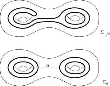
Figure 17. Type A attaching arc

Type B. The attaching arc $\alpha$ starts on a dividing curve $\gamma_{1}$, passes through a parallel dividing curve $\gamma_{2}$, and ends on $\gamma_{1}$.

Isotop $\Sigma_{0}$ through this bypass to obtain $\Sigma_{1/2}$. Let $N\subset\Sigma_{0}$ be a punctured torus regular neighborhood of the union of $\alpha$ and the annulus bounded by $\gamma_{1}$ and $\gamma_{2}$. Identify the region between $\Sigma_{0}$ and $\Sigma_{1/2}$ with $\Sigma\times[0,{1\over 2}]$ in such a way that the contact structure is $I$-invariant on $(\Sigma\setminus N)\times[0,{1\over 2}]$ and is a basic slice on $N\times[0,{1\over 2}]$. See Figure 18(A).

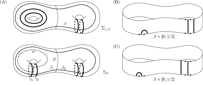
Figure 18. Type B attaching arc

Since there are more than two dividing curves on $\Sigma_{0}$, there are dividing curves contained in $\Sigma_{0}\setminus N$. Choose $\beta\subset\Sigma$ to be a closed curve formed out of an arc $\beta_{1}\subset N$ and an arc $\beta_{2}\subset\Sigma_{0}\setminus N$, where the arcs have the following properties: (i) $\beta_{1}\times\{0\}$ intersects each of $\gamma_{0}$ and $\gamma_{1}$ once, (ii) $\beta_{1}\times\{{1\over 2}\}$ intersects no dividing curves, (iii) $\beta_{2}\times\{0\}$ intersects dividing curves in $\Sigma\setminus N$, and (iv) $\beta\times\{0\}$ is efficient with respect to $\Gamma_{\Sigma_{0}}$. We may choose $\beta\times[0,{1\over 2}]$ to be convex. Since the contact structure is $I$-invariant on $(\Sigma\setminus N)\times[0,{1\over 2}]$, the dividing curves along $\beta_{2}$ are vertical. Thus there are only two possible dividing curve configurations, both of which are shown in Figure 18(B,C), and either of these forces the existence of a bypass of Type A along a subarc of $\beta\times\{0\}$.

Type C. The attaching arc $\alpha$ starts on a dividing curve $\gamma_{1}$, passes through a parallel dividing curve $\gamma_{2}$, and ends on $\gamma_{2}$ after going around a nontrivial loop.

Let $P\subset\Sigma_{0}$ be a pair-of-pants regular neighborhood of the union of $\alpha$ and the annulus bounded by $\gamma_{1}$ and $\gamma_{2}$. One of the boundary components of $P$ is a curve $\gamma$ parallel to $\gamma_{1}$ and $\gamma_{2}$, the second boundary component is a curve $B(\gamma)$ parallel to the two new dividing curves obtained from $\gamma_{1}$ and $\gamma_{2}$ after isotoping through the bypass along $\alpha$, and the third curve $\delta$ may be thought of as the nontrivial loop $\alpha$ goes around. See Figure 19.

Figure 19. Type C attaching arc

Isotop $\Sigma_{0}$ through this bypass to obtain $\Sigma_{{1/2}}$. Identify the region between $\Sigma_{0}$ and $\Sigma_{{1/2}}$ with $\Sigma\times[0,{1\over 2}]$ in such a way that the contact structure is $I$-invariant on $(\Sigma\setminus P)\times[0,{1\over 2}]$.

The proof now proceeds roughly as in the Type B case, that is, a curve $\beta$ to which the Imbalance Principle can be applied will be produced. To do this, we must consider the possible ways that $P$ can sit in $\Sigma$. See Figure 20.

Figure 20. Type C cases

Type $\mbox{C}_{\bf 1}$. $\delta$ is nonseparating and there is an arc $\beta_{2}\subset\Sigma\setminus P$ connecting $\gamma$ and $\delta$.

Let $\beta_{1}\subset P$ be an arc connecting the same points of $\gamma$ and $\delta$ and let $\beta=\beta_{1}\cup\beta_{2}$. The arcs may be chosen so that $\beta$ is efficient. If $\beta_{2}$ intersects any dividing curves, then the Imbalance Principle applied to $\beta$ (or more precisely to $\beta\times[0,{1\over 2}]$) produces a bypass of Type A. Otherwise, since $\beta$ is nonseparating, $\beta\times\{{1\over 2}\}$ is nonisolating and can be made a Legendrian divide. Again the Imbalance Principle applied to $\beta\times[0,{1\over 2}]$ produces a bypass, this time a degenerate one which can be perturbed to a bypass of Type B.

Type $\mbox{C}_{\bf 2}$. $\delta$ is nonseparating and there is an arc $\beta_{2}\subset\Sigma\setminus P$ connecting $B(\gamma)$ and $\delta$.

Let $\beta_{1}\subset P$ be an arc connecting the same points of $B(\gamma)$ and $\delta$ and let $\beta=\beta_{1}\cup\beta_{2}$. Just as in Type $\mbox{C}_{1}$, the Imbalance Principle applied to $\beta$ produces a bypass of Type A or B.

Type $\mbox{C}_{\bf 3}$. $\delta$ is separating and there is an arc contained in $\Sigma\setminus P$ connecting $B(\gamma)$ and $\gamma$.

Let $S_{1}$ be the component of $\Sigma\setminus P$ bounded by $\delta$, and let $S_{2}$ be the component with which contains $\gamma$. The genus of $S_{1}$ is greater than 0 because $\delta$ was assumed to be nontrivial. Recall $\alpha$ is a subarc of an efficient curve obtained by Proposition 6.1. If $S_{2}$ is an annulus, then the subsurface $S_{2}\cup P$ is a once-punctured torus and $\alpha$ cannot be a subarc of an efficient arc on $S_{2}\cup P$. Therefore, $S_{2}$ must have genus greater than 0 also.

Since there are more than two dividing curves on $\Sigma_{0}$, there must be dividing curves contained in $S_{1}\cup S_{2}$. Let $\beta_{1}\subset S_{1}$ be a nonseparating arc starting and ending on $\delta$, let $\beta_{2}\subset S_{2}$ be a nonseparating arc starting and ending on $\gamma$, and choose the arcs so that at least one of them has nontrivial, essential intersection with the dividing curve set. Pick two disjoint arcs in $P$ connecting the endpoints of $\beta_{1}$ to the endpoints of $\beta_{2}$ and let $\beta$ be the union of all four arcs. The Imbalance Principle produces either a bypass of Type A or, since the $\beta_{i}$ were chosen to be nonseparating, a bypass of Type $\mbox{C}_{1}$ or $\mbox{C}_{2}$.

Type $\mbox{C}_{\bf 4}$. All three curves $\delta$, $\gamma$, and $B(\gamma)$ are separating.

Let $S_{1},S_{2}$ and $S_{3}$ be, in order, the components of $\Sigma\setminus P$ these curves bound. Since each $S_{i}$ must have genus greater than 0, the proof is the same as in Type $\mbox{C}_{3}$, with one possible extra case. If all of the dividing curves of $\Sigma\setminus P$ are in $S_{3}$, then, to force $\beta\times\{{1\over 2}\}$ to be isolating, the desired $\beta$ must be produced in $S_{3}\cup P\cup S_{1}$, and the resulting bypass will lead to a reduction in the number of dividing curves on $\Sigma_{1/2}$ instead of $\Sigma_{0}$.

Thus in all possible cases a bypass (or a sequence of bypasses) can be found that will reduce the number of dividing curves by two. Hence, we can assume $\Gamma_{\Sigma_{0}}$ consists of two parallel curves. Moreover, we can assume they are nonseparating. If they are not, we can find a nonseparating curve intersecting $\Gamma_{\Sigma_{0}}$ and not intersecting $\Gamma_{\Sigma_{1}}$ and use the inbalance principle to find a bypass that transforms $\Gamma_{\Sigma_{0}}$ into a pair of nonseparating curves. ∎

Proof of Theorem 0.2.

Fix a nonseparating curve $\gamma$ on $\Sigma$. Since $f$ is pseudo-Anosov, $\gamma$ and $f(\gamma)$ are not isotopic, and we orient these curves so that $f$ preserves their orientations.

Let $\xi$ be the universally tight contact structure on $\Sigma\times[0,1]$ with $PD(\tilde{e}(\xi))=f(\gamma)-\gamma$. We claim that the contact structure obtained by gluing $\Sigma\times\{0\}$ with $\Sigma\times\{1\}$ via $f$ is universally tight. It is immediate, by the Gluing Theorem 5.1, that $2n$ copies of $\Sigma\times[0,1]$ stacked and glued together via $f$ will produce a universally tight contact structure on $\Sigma\times[-n,n]$. It follows that the glued-up contact structure on $M$ is universally tight, for any potential overtwisted disk in $M$ would lift to the $\Sigma\times\mathbb{R}$ cover of $M$ and therefore would be contained in some $\Sigma\times[-n,n]$.

To prove uniqueness, use Proposition 6.2 to choose a convex fiber $\Sigma^{\prime}$ such that $\Gamma_{\Sigma^{\prime}}=2\gamma^{\prime}$, where $\gamma^{\prime}$ is some nonseparating curve, and split $M$ along $\Sigma^{\prime}$ to obtain $\Sigma^{\prime}\times I$. Since $f$ is pseudo-Anosov, $\Gamma_{\Sigma^{\prime}\times\{0\}}\not=\Gamma_{\Sigma^{\prime}\times\{1\}}$, and therefore $\Sigma^{\prime}\times I$ contains a basic slice by Lemma 5.5. It follows from Proposition 5.2 that a new convex fiber $\Sigma^{\prime\prime}$ may be chosen such that $\Gamma_{\Sigma^{\prime\prime}}=2\gamma$.

Let us assume for simplicity that $\gamma$ and $f(\gamma)$ are not homologous. (The general case is no harder, but requires the use of Lemma 5.9, and is harder to state.) By Theorem 0.1, there are four possibilities for $\xi_{\Sigma^{\prime\prime}\times I}$ with distinct relative Euler classes $\pm f(\gamma)\pm\gamma$. If the relative Euler class is $\pm f(\gamma)+\gamma$, then $\Sigma^{\prime\prime}\times[0,1]$ contains a slice $\Sigma^{\prime\prime}\times[0,{1\over 2}]$ where $\Gamma_{\Sigma^{\prime\prime}\times\{{1\over 2}\}}=2\gamma$ and the slice has relative Euler class $2\gamma$. By peeling this slice and reattaching using $f$, we obtain $\Sigma^{\prime\prime}\times[{1\over 2},1]\cup f(\Sigma^{\prime\prime}\times[0,{1\over 2}])$. It follows that for any given tight contact structure on $M$, there always exists a convex fiber $\Sigma$ such that the restriction of $\xi$ to $\Sigma\times I$ (obtained by cutting along $\Sigma$) has relative Euler class $\pm f(\gamma)-\gamma$.

It is clear, from the location of bypasses on the $-f(\gamma)-\gamma$ contact structure on $\Sigma\times I$ (or by Proposition 5.6), that gluing by $f$ produces an overtwisted contact structure on $M$. Thus $\xi$ on $M$ can always be split to have relative Euler number $f(\gamma)-\gamma$ and the uniqueness on $M$ follows from Theorem 0.1.

It remains to discuss weak fillability. First note that there exists a $C^{0}$-small perturbation of the fibration into a universally tight contact structure $\xi$, by a result of Eliashberg and Thurston [7]. Since the Euler class evaluated on the fiber is unchanged under the perturbation, we have, say, $\langle e(\xi),\Sigma\rangle=-(2g-2)$. By the uniqueness which we just proved, the unique extremal tight contact structure on $M$ with $\langle e,\Sigma\rangle=-(2g-2)$ is isotopic to $\xi$. Now, to prove weak symplectic fillability, we construct a symplectic 4-manifold $(X,\omega)$ with $\partial X=M$ for which $\omega|_{T\Sigma}>0$ (for all fibers $\Sigma$). Since $\xi$ is close to the fibration, we would then be done. The construction of $X$ is relatively straightforward from the Lefschetz fibration perspective, once we observe that any element $f:\Sigma\rightarrow\Sigma$ of the mapping class group of a closed surface $\Sigma$ can be written as a product of positive Dehn twists. (For more details on symplectic Lefschetz fibrations, see, for example [13].) We take a symplectic Lefschetz fibration $X\rightarrow D^{2}$ with generic fiber $\Sigma$ and a singular fiber for each positive Dehn twist in the product expression. We then see that $\partial X=M$ has the desired monodromy and each fiber $\Sigma$ is a symplectic submanifold. ∎

Acknowledgements. The first author gratefully acknowledges the American Institute of Mathematics and IHES for their hospitality. The authors also thank Emmanuel Giroux for suggesting that Theorem 0.2 might be true, and John Etnyre for discussions which led to Proposition 6.2.

References

- [1] D. Bennequin, Entrelacements et équations de Pfaff, Astérisque 107-108 (1983), 87–161.
- [2] V. Colin, Chirurgies d’indice un et isotopies de sphères dans les variétés de contact tendues, C. R. Acad. Sci. Paris Sér. I Math. 324 (1997), 659–663.
- [3] V. Colin, Recollement de variétés de contact tendues, Bull. Soc. Math. France 127 (1999), 43–69.
- [4] V. Colin, Une infinité de structures de contact tendues sur les variétés toroïdales, Comment. Math. Helv. 76 (2001), 353–372.
- [5] V. Colin, E. Giroux and K. Honda, in preparation.
- [6] Y. Eliashberg, Contact 3-manifolds twenty years since J. Martinet’s work, Ann. Inst. Fourier (Grenoble) 42 (1992), 165–192.
- [7] Y. Eliashberg and W. Thurston, Confoliations, University Lecture Series 13, Amer. Math. Soc., Providence, RI, 1998.
- [8] D. Gabai, Foliations and the topology of -manifolds, J. Differential Geom. 18 (1983), 445–503.
- [9] E. Giroux, Convexité en topologie de contact, Comment. Math. Helv. 66 (1991), 637–677.
- [10] E. Giroux, Une infinité de structures de contact tendues sur une infinité de variétés, Invent. Math. 135 (1999), 789–802.
- [11] E. Giroux, Structures de contact en dimension trois et bifurcations des feuilletages de surfaces, Invent. Math. 141 (2000), 615–689.
- [12] E. Giroux, Structures de contact sur les variétés fibrées en cercles au-dessus d’une surface, Comment. Math. Helv. 76 (2001), 218–262.
- [13] R. Gompf and A. Stipsicz, 4-manifolds and Kirby calculus, Graduate Studies in Mathematics 20, Amer. Math. Soc., Providence, RI, 1999.
- [14] K. Honda, On the classification of tight contact structures I, Geom. Topol. 4 (2000), 309–368.
- [15] K. Honda, On the classification of tight contact structures II, to appear in J. Differential Geom.
- [16] K. Honda, Gluing tight contact structures, to appear in Duke Math. J.
- [17] K. Honda, W. Kazez and G. Matić, Tight contact structures and taut foliations, Geom. Topol. 4 (2000), 219–242.
- [18] K. Honda, W. Kazez and G. Matić, Convex decomposition theory, Internat. Math. Res. Notices 2002, 55–88.
- [19] N. Ivanov, Mapping class groups, to appear in the Handbook of Geometric Topology.
- [20] Y. Kanda, The classification of tight contact structures on the 3-torus, Comm. Anal. Geom. 5 (1997), 413–438.
- [21] Y. Kanda, On the Thurston-Bennequin invariant of Legendrian knots and non exactness of Bennequin’s inequality, Invent. Math. 133 (1998), 227–242.